Foreigners Knocking on the Door: Trade in China During

the Treaty Port Era

By Wolfgang Keller, Javier Andres Santiago, and Carol H. Shiue∗

Draft: January 4, 2015

We employ a new, commodity-level dataset on the flow of goods be-

tween fifteen major treaty ports to estimate a general-equilibrium

trade model for China around the year 1900. The distribution

of welfare effects depends critically on each port’s productivity,

China’s economic geography because it affects trade costs, and the

extent of regional diversity in production because this affects the po-

tential gains from trade. We utilize this framework to quantify the

size and distribution of welfare effects resulting from new technol-

ogy and lower trade costs that came with the treaty ports. Find-

ings show that domestic markets resulted in ripple effects which

transmitted the effect of the international trade opening beyond the

foreign concessions. However, because differences in relative pro-

ductivity across regions were relatively low, the welfare gains from

domestic trade improvements were limited. Keywords: domestic

trade, welfare gains, 19th century China

∗ Keller: University of Colorado, CEPR, NBER, CESifo, wolfgang.keller@colorado.edu. Andres Santi-ago: University of Colorado, javier.andressantiago@colorado.edu. Shiue: University of Colorado, CEPR,NBER, CESifo, shiue@colorado.edu. We thank Greg Clark, Kris Mitchener, Noam Yuchtman, and work-shop participants at the All UC Group in Economic History Conference 2015 for useful comments. BillRidley provided excellent research assistance. Keller and Shiue gratefully acknowledge support by theNational Science Foundation (grant SES 1124426).

1

China’s economic development has taken major turns over the last couple of cen-

turies. From a relatively prosperous worldwide standing during the Song era

(960-1279), China saw Western European countries surging ahead in the great

divergence of the late 18th century. Over the last twenty-five years, China expe-

rienced rates of growth of close to 10% per year, doubling per-capita income more

rapidly than in any other sizable country in world history. While recent research

has begun to shed light on these turning points, still very little is known on the

legacy of China’s 19th century opening.

Starting in mid-19th century, under military action from Western countries, China

opened an increasing number of ports to foreign traders. In this paper we examine

the implications of this opening for China’s internal trade and welfare. Treaty

ports were the conduits of goods, but they were also the carriers of Western

influence. Foreigners introduced steam ships to China, dredged harbors, built

lighthouses, and under the Chinese Maritime Customs authority collected not

only tariff revenue, but also data on goods trade, weather, and other aspects of

the Chinese economy.

We employ a new, commodity-level dataset for fifteen major treaty ports to es-

timate a general-equilibrium trade model for China around the year 1900. After

the collapse of the Qing dynasty in 1911, a small but significant modern sector

based on factory production started to grow at rates well over 2% and lasted until

the Japanese invasion of 1937 (Chang 1969). This industrialization centered on

the treaty ports. While it was started by the foreign presence, the strength of

domestic market expansion contributed to its growth. What has been less clear is

whether the developments of the 1912-1937 period, and more generally the open-

ing of trade that precipitated these developments, had wider effects that went

beyond the treaty ports.

We show that the distribution of welfare effects depends critically on each port’s

productivity, China’s economic geography because it affects trade costs, and the

extent of regional diversity in production because it shapes the potential gains

2

from trade. We utilize this framework to quantify the size and distribution of

welfare effects resulting from new technology and lower trade costs that came with

the treaty ports. Specifically, a 20% increase in Shanghai’s productivity raises

welfare in Shanghai by about 1.5%; because of trade, however, Shanghai’s gains

are only part, about 40%, of the total welfare gains. Another 28% of the welfare

gains accrue to Ningbo, Chinkiang, and Wuhu, located in the geographic vicinity

of Shanghai. Because factor costs, income, and production patterns respond

endogenously, welfare in some ports can actually fall when Shanghai’s technology

improves, as it does in the relatively distant Tianjin . We also study the effects

of changes in trade costs on welfare.

There are two main findings. First, we show that through trade, a change in

any one of the treaty ports has ripple effects throughout China; it is not bottled

up within the foreign concession. These effects, conditioned by China’s economic

geography, yield a new estimate of the extent to which China was influenced by

foreign contact, and is based on commodity-level trade data. Second, across China

during the treaty port era, the evidence for regional diversity in productivity

across goods is relatively small; smaller at any rate than for trade in manufactured

goods across high-income countries in the late 20th century. This puts a lid on the

aggregate size of welfare gains because differences in productivity across goods–

comparative advantage–is the source of the gains from trade in our framework.

This paper contributes to a small but growing literature on China’s trade during

the treaty port era (1842 to 1943). An important contribution is Mitchener and

Yan (2014) who study the factor price implications of China’s foreign trade during

the early 20th century.1 China’s substantial foreign trade notwithstanding, the

size of China’s domestic trade exceeded it by far. In 1904, for example, Shang-

hai’s exports to Great Britain were similar in size to Shanghai’s exports to the

Shandong treaty port of Yantai (Chefoo), while exports from Tianjin (Tientsin) to

1Keller, Li, and Shiue (2011, 2013) provide overviews of China’s foreign trade during the treaty portera all the way to today. China’s trade statistics during the treaty port era are discussed in Hsiao (1974)and Lyons (2003).

3

Shanghai were about five times the size of Tianjin’s exports to all foreign countries

combined.2 By shifting the focus on China’s internal trade we observe the effects

of greater international integration within the country, something that is possible

only in rare cases.3 Our analysis complements earlier work on China’s internal

trade in this era (Kose 1994, 2005; Keller, Li, and Shiue 2012) by quantifying the

size and and analyzing the structure of the welfare gains from trade.

This research also contributes to the re-assessment of the broader implications

that Western pressure had on China during the 19th and early 20th century.

Earlier views on the impact on China ranged from very negative to mildly benign

(see the overview in Dernberger 1975).4 While the intrusion of the West has often

been seen as detrimental to China’s economic development, some authors consider

positive demonstration effects (Feuerwerker 1983). There were also changes in

traditional sectors (Rawski 1989, Richardson 1999). Recent work has begun to

see the treaty ports in a more positive light (Keller, Li, and Shiue 2011, So and

Myers 2011), noting in particular that city size grew more rapidly in treaty ports

than in other cities (Jia 2013). Given China’s size, did the developments in the

treaty ports matter for China more broadly? We provide an initial estimate on

the geographic scope of the West’s impact in China from the point of view of a

general-equilibrium trade model.5

Finally, we contribute to the analysis of trade by asking how a general-equilibrium

model can capture the welfare gains from trade. While much progress has been

made with Heckscher-Ohlin models (O’Rourke and Williamson 1994, 1999; Mitch-

ener and Yan 2014), when the size of the country suggests that economic geogra-

phy aspects could be important, as in the case of a large country such as China,

our Ricardian framework based on Eaton and Kortum (2002) is preferable to a

2See CMC (2001a), Vol. 39. These figures underestimate the relative size of domestic trade becauseit ignores domestic trade outside of the realm of the Chinese Maritime Customs service (see below).

3The paucity of information on internal trade is closely related to the absence of internal trade taxes inmany countries; e.g. the Import-Export Clause, Article 1, Section 10, Clause 2 of the U.S. Constitution.

4See also the accounts of Morse (1926) and Fairbank (1978).5The effect of China’s 19th century opening on her capital markets is examined in Keller and Shiue

(2015).

4

Heckscher-Ohlin framework because it remains highly tractable in the presence of

trade costs, generating bilateral trade predictions in a multi-region setting. This

allows us to investigate in a counterfactual setup the size and structure of welfare

effects as well as the factors which were central in explaining these outcomes. This

Ricardian framework has been applied for welfare analysis to trade of regions and

countries, multinational activity, and migration (see the review in Costinot and

Rodriguez-Clare 2013). We add China to the short list of countries for which his-

torical analyses exist.6 In particular, our paper complements Donaldson’s (2015)

analysis of agricultural income gains due to railroad introduction in India by a

focus on trade via ships of a broader set of commodities. While the quality of our

data on China does not match that for British India, we know the precise volume

of trade on ships, in contrast to British India where only data on the location of

railroad tracks and the total trade volume is available.

The paper is structured as follows. The following section gives a brief summary

of the historical setting, with more details given in Fairbank (1978); Cassel (2012)

and Keller and Shiue (2012, 2014, 2015). The model is described in section 3, with

more details given in Eaton and Kortum (2002). Next is a description of the data,

with additional information provided in the Appendix. In section 5 we present

the empirical results, beginning with the estimation of key parameters, followed

by welfare calculations based on counterfactual analysis. The paper concludes

with a summary and discussion of future research directions in section 6.

I. Historical Background: Trajectories from the Past

After her defeat in the First Opium War (1840 – 1842), China signed the Treaty of

Nanjing (1842) which expanded the rights of Western countries to trade at a total

of five Chinese ports, four more than the one (Canton) that they had been allowed.

Other stipulations included that Hong Kong would become a British colony, and

that foreigners would be subject to the laws of their own countries, as opposed to

6On India, see Donaldson (2015), while for Argentina, see Fajgelbaum and Redding (2015).

5

Chinese law (extraterritoriality). Additional ports were opened to trade with the

West in subsequent years. Given that the post-1842 increase in trade did not live

up to Western expectations, and that trade taxes went largely unpaid during the

Taiping Rebellion (1850-64), in the year 1854 it was decided that China’s customs

system would be run by Western officials who formally would be employed by

China’s central government. The organization that was founded for this task

was the Chinese Maritime Customs Service (CMCS; Imperial Maritime Customs

Service before 1911), with Horatio Nelson Lay as its first leader. Operations of

the CMCS began in full in the year 1859 in Shanghai, with other ports following

over time. Robert Hart became Inspector-General of the CMCS in the year 1863.

His influence was shaping China’s trade opening for decades to come.

While this paper is focused on the welfare effects of China’s domestic trade around

the turn of the century, given the unprecedented growth of trade and foreign direct

investment in China since 1978 it is important to ask how the 19th century fits

in with China’s long-run development (see also Brandt, Ma, and Rawski 2014).

For the following analysis we focus on Shanghai, which is the largest port in the

world today by several measures (see Keller, Li, and Shiue 2013).

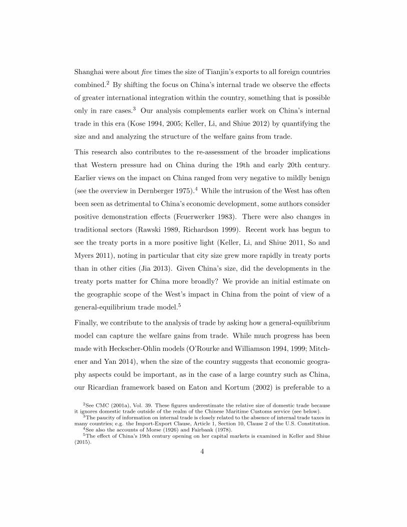
We begin by considering foreign trade. In Figure 1, we show Shanghai’s exports

to the European continent between 1865 and 2009. Extrapolating the trend from

1865 to 1900, we see that the level of Shanghai’s exports in the early 2000s was

close to what one would have predicted based on the 19th century trend. Figure

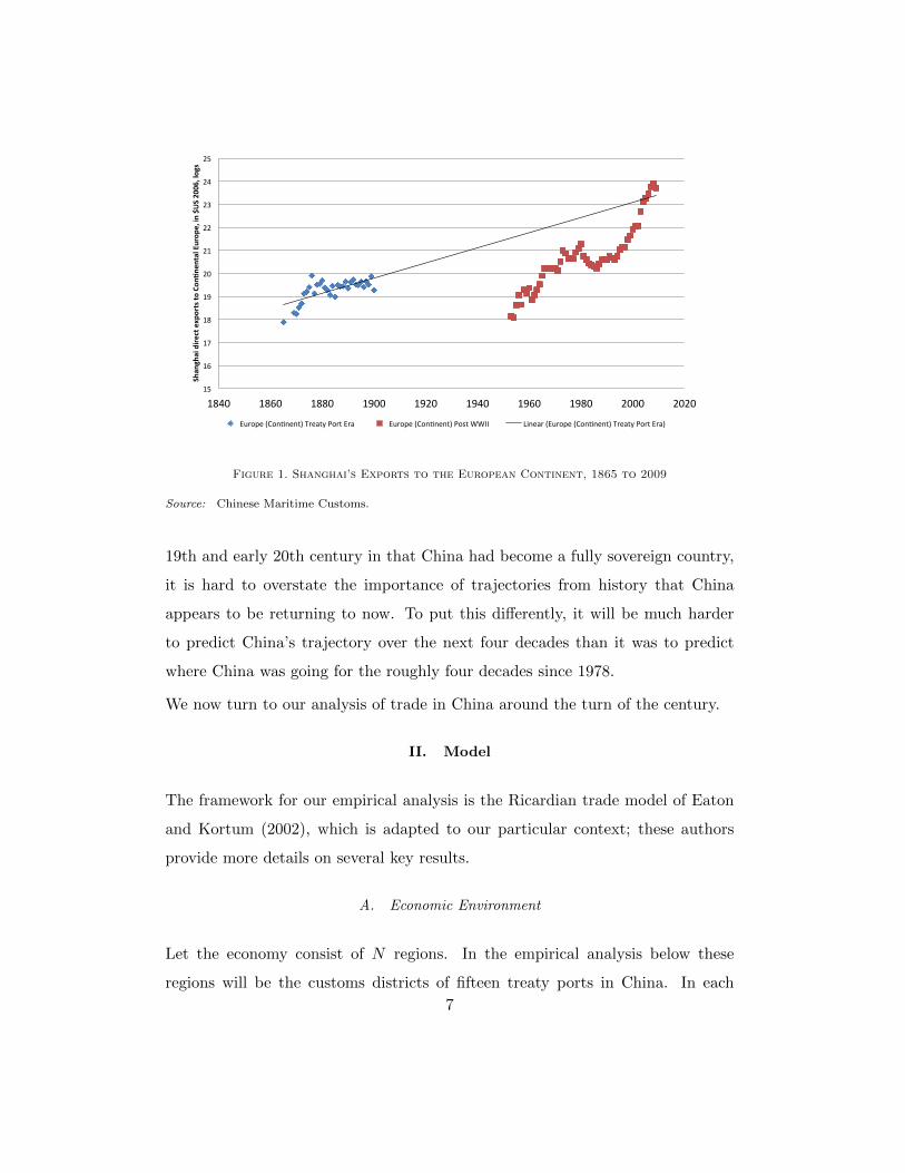
2 shows that French foreign direct investment (FDI) in Shanghai is well below

what a simple extrapolation of the 1872-1921 trend would yield.7 This might be

explained in part because outward globalization—exports—is politically easier

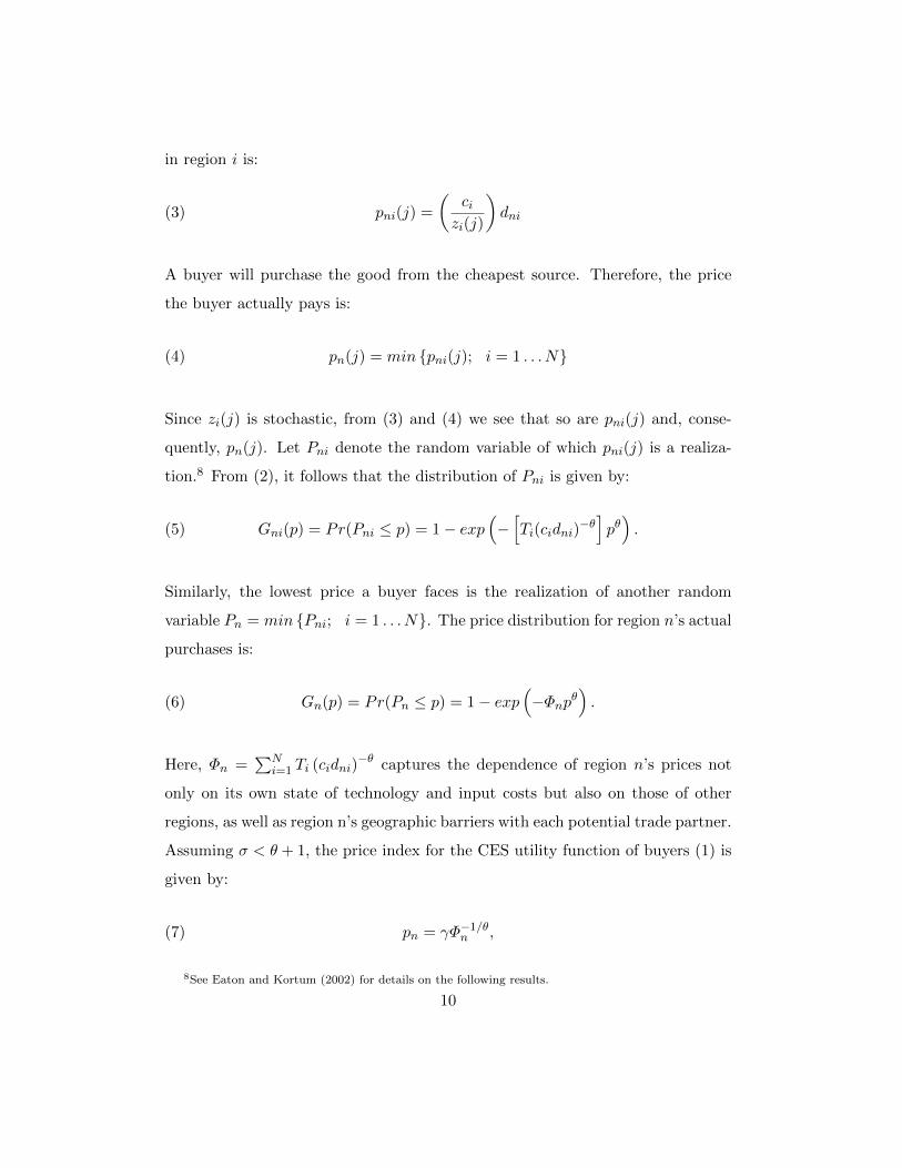
than globalization in terms of inward FDI. At the same time, Figure 3 shows

that the number of Germans in Shanghai today is quite close to what one would

expect based on extrapolating the 19th century trend.

Overall, these findings suggest that although the post-1949 era differs from the

7On our measures of FDI in the two periods, see Keller, Li, and Shiue (2013).

6

Shanghai’sExportstotheEuropeanContinent,1865to2009

15

16

17

18

19

20

21

22

23

24

25

1840 1860 1880 1900 1920 1940 1960 1980 2000 2020

Shan

ghaidire

ctexportsto

Con

2nen

talEurop

e,in$US2006,logs

Europe(Con5nent)TreatyPortEra Europe(Con5nent)PostWWII Linear(Europe(Con5nent)TreatyPortEra)

Figure 1. Shanghai’s Exports to the European Continent, 1865 to 2009

Source: Chinese Maritime Customs.

19th and early 20th century in that China had become a fully sovereign country,

it is hard to overstate the importance of trajectories from history that China

appears to be returning to now. To put this differently, it will be much harder

to predict China’s trajectory over the next four decades than it was to predict

where China was going for the roughly four decades since 1978.

We now turn to our analysis of trade in China around the turn of the century.

II. Model

The framework for our empirical analysis is the Ricardian trade model of Eaton

and Kortum (2002), which is adapted to our particular context; these authors

provide more details on several key results.

A. Economic Environment

Let the economy consist of N regions. In the empirical analysis below these

regions will be the customs districts of fifteen treaty ports in China. In each

7

FrenchFDIinShanghai,1872-2009

0

1

2

3

4

5

6

7

1860 1880 1900 1920 1940 1960 1980 2000 2020

Nooffo

reignfund

edfirm

s,logs

FranceTreatyPortEra Francelate20thc Linear(FranceTreatyPortEra)

Figure 2. French FDI in Shanghai

Source: Chinese Maritime Customs.

region, competitive firms produce a continuum of goods j ∈ [0, 1]. Technologies

differ across regions and goods, with region i’s efficiency in producing good j

denoted by zi(j). Regions can trade with each other, though trade is costly.

Specifically, trade costs are modeled as “iceberg” costs, dni, where n and i denote

destination (importer) and source (exporter) region, respectively. Trade costs of

dni mean that d units of the good have to be shipped from i in order for one unit

to arrive in region n. As it is customary, we set dii = 1 ∀i and dni > 1 if n 6= i.

Goods can be purchased in an amount Q(j) for final consumption by consumers,

or as intermediate inputs by firms. Consumers maximize a CES utility function:

(1) U =

[ˆ 1

0Q(j)(σ−1)/σ

]σ/(σ−1)

subject to region n’s total spending, Xn, where σ > 0 is the elasticity of substi-

tution between each pair of goods.

Region i’s efficiency in the production of good j, zi(j), is stochastic and drawn

8

4

5

6

7

8

9

10

1860 1880 1900 1920 1940 1960 1980 2000 2020

Num

bero

fGerman

reside

nts,logs

GermanyTreatyPortEra Germany2000s Linear(GermanyTreatyPortEra)

GermanPopulationinShanghai,1872to2009

Figure 3. German Population in Shanghai

Source: Chinese Maritime Customs.

from a Frechet distribution with cumulative distribution function:

(2) Fi(z) = e−Tiz−θ

The parameter Ti > 0 describes region i’s specific technology. A higher value of

Ti increases the probability of drawing a higher level of technology, and hence

Ti is a measure of absolute advantage. The parameter θ > 1 is inversely related

to the variance of the distribution. A lower value of θ indicates a higher degree

of heterogeneity in relative productivity. Thus, we refer to θ as the comparative

advantage parameter.

Let ci denote the input cost of production in region i . With competitive firms, a

constant-returns-to-scale technology, and the above-mentioned geographic barri-

ers to trade, the price a buyer in region n would pay for 1 unit of good j produced

9

in region i is:

(3) pni(j) =

(cizi(j)

)dni

A buyer will purchase the good from the cheapest source. Therefore, the price

the buyer actually pays is:

(4) pn(j) = min {pni(j); i = 1 . . . N}

Since zi(j) is stochastic, from (3) and (4) we see that so are pni(j) and, conse-

quently, pn(j). Let Pni denote the random variable of which pni(j) is a realiza-

tion.8 From (2), it follows that the distribution of Pni is given by:

(5) Gni(p) = Pr(Pni ≤ p) = 1− exp(−[Ti(cidni)

−θ]pθ).

Similarly, the lowest price a buyer faces is the realization of another random

variable Pn = min {Pni; i = 1 . . . N}. The price distribution for region n’s actual

purchases is:

(6) Gn(p) = Pr(Pn ≤ p) = 1− exp(−Φnpθ

).

Here, Φn =∑N

i=1 Ti (cidni)−θ captures the dependence of region n’s prices not

only on its own state of technology and input costs but also on those of other

regions, as well as region n’s geographic barriers with each potential trade partner.

Assuming σ < θ + 1, the price index for the CES utility function of buyers (1) is

given by:

(7) pn = γΦ−1/θn ,

8See Eaton and Kortum (2002) for details on the following results.

10

whereγ is defined as γ ≡[Γ(θ+1−σ

θ

)]1/(1−θ), and Γ is the Gamma function. This

price index will be critical for the welfare analysis. Two additional results are key

to this.

First, one can show that the probability that region i is the cheapest source of a

good for destination n is given by:

(8) πni =Ti (cidni)

−θ

Φn

Since there is a continuum of goods we can apply the law of large numbers, and

(8) also gives the fraction of goods region n buys from i.

Second, it can be shown that the price distribution (6) does not depend on the

source region. Thus, since the price of a good purchased by a region n buyer does

not vary with the source, the share of region n’s expenditure on goods produced

in region i must be equal to the fraction of goods bought from that region, given

by (8):

(9)Xni

Xn= πni =

Ti (cidni)−θ∑N

k=1 Tk (ckdnk)−θ

where Xni is region n’s expenditure on region i’s goods and Xn =∑N

i=1Xni is

region n’s total expenditure.

Multiplying both sides of (9) by Xn gives that equation a gravity interpretation:

bilateral trade Xni is increasing in the importer region’s total expenditure. It is

also increasing in the size of the exporter region, related to its state of technology,

Ti. Finally, it is decreasing in the size of geographic barriers, dni. Thus, the model

captures the effects of technology and geography on bilateral trade.

11

B. Model Equilibrium

We assume that production takes place by combining labor and intermediate

inputs. Region i’s input cost is then

(10) ci = wβi p1−βi

where wi is the wage in region i and pi is region i’s price index as given by (7).

Labor’s share in production is given by the parameter β, 0 < β < 1.

Substituting (10) into the expression for Φ, and the result into (7) yields a system

of equations that relates each region’s price index to wages as well as technology

and comparative advantage parameters in all other regions:

(11) pn = γ

[N∑i=1

Ti

(wβi p

1−βi dni

)−θ]

Also, substituting (10) into (9), we can express trade shares as a function of wages

and the parameters of the model:

(12)Xni

Xn= πni = Ti

(γdniw

βi p

1−βi

pn

)−θ

To determine the equilibrium in the labor market, we assume that workers are

immobile between the sector producing manufacturing goods, modeled so far, and

another sector producing non-manufacturing goods.9 We make this assumption

both because it is not unreasonable for this historical setting, and because it

gives us a conservative estimate (lower than the mobile labor case), which seems

reasonable given the debate on the welfare impact of the foreign opening on China.

Manufacturing labor income in region i is given by labor’s share in the value of

that region’s total sales of manufacturing products (to local buyers and to other

9We use the term manufacturing for brevity; as will become clear below it also includes agriculturaland other goods.

12

regions):

(13) wiLi = βN∑n=1

πniXn

where Li denotes the number of workers.

Total expenditures in manufacturing are given by:

(14) Xn =1− ββ

wnLn + αYn

where Yn denotes aggregate final expenditure, and α is the fraction spent on

manufacturing products. Final expenditure is the sum of value added in man-

ufacturing, YMn , and income generated in the non-manufacturing sector, Y NM

n .

We assume that trade costs in non-manufacturing are negligible, so that it can

be used as our numeraire.

Combining (13) and (14), we obtain the labor-market condition:

(15) wiLi =

N∑n=1

πni[(1− β + αβ)wnLn + αβY NM

n

]

Equations (11), (12), and (15) characterize the equilibrium of the model and can

be solved numerically for prices, trade shares, and manufacturing wages. These

allow us to construct a measure of overall welfare at the regional level, given by

real GDP

(16) Wn =Ynpαn

where, since non-manufactures are taken as numeraire, pαn denotes the price level

in region n. Our counterfactual analyses in Section 5 look at the effects of chang-

ing technology and trade barriers on welfare as defined by equation (16). In the

following section we describe the data, followed by the estimation of the param-

13

eters of the model.

III. Data

We examine China’s internal trade around the year 1900. This section summa-

rizes the data that will be employed, with more details given in the Appendix.

The analysis includes fifteen of China’s foreign treaty ports, which are listed in

Table 1 according to the ports’ names as recorded by the British CMC service

as well as the English transliteration of the port name (in Pinyin), and the 20th

century provincial jurisdiction. The port of Guangzhou in Guangdong province,

for example, is called Canton in the Maritime Trade publications. These treaty

ports are defined on the basis of the customs district of each port, which includes

not only the port but also the surrounding area. One might therefore prefer to

think of the treaty ports as regions; we will use the terms ports and regions inter-

changeably. Our choice of these 15 ports is based on their importance for China’s

maritime trade. The three largest ports during the 19th century were Shanghai,

Wuhan (Hankow), and Tianjin (Tientsin).

Figure 4 shows the locations of the fifteen ports. The figure shows that we cover

broad regions of China, mainly along its coast but also along the Yangzi river.

The distance between Canton (Guangzhou) and Newchwang (Niuzhuang), which

are located in Guangdong and Liaoning province, respectively, is about 2,700

kilometers.

The Maritime Trade statistics include only the trade that went through the Chi-

nese Maritime Customs Service (CMC). Although our analysis excludes land-

based trade, the amount of other water-borne trade in China (which was covered

by the Native Customs system but not by the CMC) was small in comparison

to the CMC portion (see CMC 2001a).10 While land-based trade was significant,

especially over short-distances, there is no reason to believe that the omission of

land-based trade creates a bias in our analysis.

10The importance of railroads in China around the year 1900 was still quite limited.

14

Table1—

SummaryStatistics

19th

c.P

rovin

ceP

inyin

Wag

eC

hin

ese

For

eign

Lab

orT

otal

Tot

al

Port

Nam

eP

op.

size

Pop

.si

zeF

orce

Exp

orts

Imp

orts

Am

oyF

uji

an

Xia

men

1.00

011

4,00

01,

685

59,9

2566

0,41

93,

018,

895

Can

ton

Gu

an

gdon

gG

uan

gzh

ou1.

534

900,

000

951

466,

692

3,92

1,65

916

,279

,439

Ch

efoo

Sh

and

on

gY

anta

i0.

857

75,0

0083

839

,284

8,68

6,66

66,

354,

247

Ch

inkia

ng

Zh

ejia

ng

Zh

enji

ang

0.85

116

7,00

022

986

,625

6,29

0,75

45,

818,

371

Fooch

owF

uji

an

Fu

zhou

0.89

362

4,00

081

832

3,65

53,

915,

828

1,54

3,33

1H

anko

wH

ub

eiH

an

kou

0.98

787

0,00

01,

828

451,

607

57,0

00,3

7111

,211

,702

Ich

ang

Hub

eiY

ich

ang

1.20

045

,000

8823

,356

1,30

4,92

11,

677,

188

Kia

och

owS

han

don

gQ

ingd

ao

1.25

312

2,00

079

863

,609

5,31

5,95

477

3,32

1K

iukia

ng

Jia

ngxi

Jiu

jian

g0.

906

36,0

0022

818

,766

12,2

09,8

971,

293,

445

New

chw

an

gL

iaon

ing

Niu

zhu

an

g0.

985

50,0

002,

004

26,9

3810

,356

,791

6,44

4,67

8N

ingp

oZ

hej

ian

gN

ingb

o0.

942

260,

000

266

134,

818

7,91

8,60

73,

093,

938

Sh

angh

aiJia

ngs

uS

han

ghai

0.94

265

1,00

019

,294

347,

212

28,2

89,3

1990

,527

,891

Sw

ato

wG

uan

gd

ong

Sh

anto

u1.

136

48,0

0059

625

,173

8,66

0,62

015

,100

,431

Tie

nts

inZ

hil

iT

ian

jin

1.03

675

0,00

04,

542

390,

852

12,8

09,6

9115

,837

,388

Wu

hu

An

hu

iW

uhu

0.91

912

2,00

015

163

,274

13,2

67,6

121,

634,

844

Source:

Sel

ecti

on

from

“L

ist

of

Tre

aty

Port

s,E

tc.,

inC

hro

nolo

gic

al

Ord

er”

inIn

spec

tor

Gen

eral’s

Cir

cula

rs,

1893

to1910,

“D

ocu

men

tsIl

lust

rati

ve

of

the

Ori

gin

,D

evel

op

men

t,an

dA

ctiv

itie

sof

the

Ch

ines

eM

ari

tim

eC

ust

om

sS

ervic

e”,

Volu

me

2.

Wage

see

Ap

pen

dix

A;

Ch

ines

ep

op

ula

tion

CM

C(2

001a),

varo

us

volu

mes

;F

ore

ign

pop

ula

tion

as

aver

age

for

yea

rs1901

an

d1911,

from

CM

C(2

001b

);la

bor

forc

eis

51.8

%of

pop

ula

tion

(Liu

an

dY

eh1965);

tota

lex

port

san

dim

port

s(e

xcl

ud

ing

pu

rch

ase

sfr

om

self

)fo

ryea

r1904

from

CM

C(2

001a),

vol.

39

an

d40.

15

Figure 4. The 15 Treaty Ports in the Analysis.

Source: Authors’ map.

A. Trade data

Two types of trade data are employed in the analysis: first, commodity-level

multilateral trade at each of the fifteen regions, and second, the aggregate bilateral

trade between the regions. Our analysis focuses on imports and exports of Chinese

products, referred to in the Maritime statistics as ’native goods’. The commodity-

level trade data is employed to estimate local prices, defined as the unit value of

a range of goods at each port. The price difference for a given good between two

regions provides an upper bound for the trade costs between these two regions.

Before we turn to that, the following discusses aggregate bilateral trade of our

regions (see Figure 5).

16

Figure 5. Bilateral Trade between Regions

Source: Calculated from CMC trade data.

This figure shows the matrix of bilateral trade, with the thickness of each line

proportional to the size of the flow. Exports are shown in the color of the region

itself and are offset towards the center of the figure. Hankow exports a large

amount of its production to Shanghai, for example, while Tientsin’s imports from

Hankow are smaller than Tientsin’s imports from Shanghai.

Importantly, the trade volumes shown in Figure 5 are locally produced in each

of the fifteen regions. The Maritime Trade statistics are exceptional in that

they provide information on re-export trade separately from local-origin trade.

17

Shanghai, in particular, re-exports goods from other Chinese regions at a level

that exceeds its exports of local origin. If each region would export to every other

region, Figure 5 would show 15 x 14 trade flows; however, 22% are equal to zero.11

Also note that this trade is not balanced in the year 1904; we do not examine

issues of intertemporal trade in the model.

The final step in our discussion of aggregate trade data concerns the trade of

region i with itself. Because we do not have information on production in region

i, we cannot follow the usual approach of obtaining region i ’s purchases from itself

as its production minus total exports. Instead, we first run a gravity equation

using all bilateral data on trade between regions i and j. With the coefficient on

distance on hand, the purchase of region i from itself could be estimated by the

predicted value of trade given a zero value of distance. Following the empirical

gravity literature, however, we modify this approach to account for the size of

region i (which is not zero) as its internal distance (see Appendix C).

Turning to the commodity-level trade data, Figure 6 provides some detail on the

most important commodities in four regions, as well as a comparison between the

size of domestic and foreign trade at the commodity level. With the exception of

Silk piece goods out of Canton and Raw cotton from Shanghai, domestic trade

is larger than foreign trade. Furthermore, it is clear that foreign trade is less

important than domestic trade in ports other than Shanghai.

The commodity-level trade data in this paper is employed to estimate the key

parameter θ from examining price differences across ports. For this purpose we

picked 26 commodities that are traded between virtually all fifteen regions. These

commodities include coal, matches, rice, cotton, leather, silk pieces, among other

goods. In Table 2 we show the average price difference in each region versus all

other regions. With the exception of Tianjin, the average price differences are not

far from zero. This is consistent with the hypothesis that at least across these 26

11In the estimation we add one before taking logs; using Poisson-type estimation models does notchange our main results.

18

Figure 6. Five Key Commodities, by Region

Source: Chinese Maritime Customs’ Decennial Reports, CMC (2001b).

commodities, most regions are low-cost for some and high-cost for other products.

B. Wages

We obtain information on wages paid in the treaty ports from the Chinese Mar-

itime Customs’ Decennial Reports, CMC (2001b). These sources cover our fifteen

regions over years 1892 to 1921; the director of the customs station in each port

was asked to report about typical wages for particular occupations paid in his

district. Occupations include both more and less skilled jobs such as painters,

coolies, silk weavers, and manual laborers. The most frequent records are avail-

able for carpenters. Given the relatively small number of observations (n = 294),

19

Table 2—Bilateral Price Differences on 26 Commodities

Region Avg. Percent Difference Region Avg. Percent Difference

Amoy 2.4 Kiukiang 8.7Canton -0.2 Newchwang 0.1Chefoo -0.4 Ningpo 1.9Chinkiang -1.3 Shanghai 1.4Foochow -1.6 Swatow 9.9Hankow -0.1 Tientsin 24.5Ichang 1.3 Wuhu -0.5Kiaochow -4.3

Source: Chinese Maritime Customs’ Decennial Reports, CMC (2001b).

we have estimated a region’s wage from a hedonic regression across all ports (in-

cluding occupation and year fixed effects). This is discussed further in Appendix

A.

Wages across China around 1900 varied to some degree; the lowest wage wi is

obtained for Chinkiang at 0.85, the highest for Canton at 1.5; the units for these

figures is payment for a day’s work of a carpenter in silver taels. We have also

examined the robustness of our findings using alternative regional wages estimated

from a subset of the Decennial Reports wage data together with a polynomial in

longitude and latitude, finding similar results.

C. Labor Force and Gross Product

We estimate the labor force in each region, Li, by applying estimates of the

labor force participation in China from Liu and Yeh (1959) to figures on the

Chinese and foreign population living in each region, from CMC (2001a,b). Our

GDP estimates are equal to the wage bill in each region, estimated as wiLi, plus

the contribution from land, which is estimated based on Perkins (1969).12 See

Appendix B for details.

12We employ Perkins’ (1969) estimates of the value of provinvial agricultural production across thirteenproducts, and use data on the fraction of people living in each region i relative to total provincialpopulation to apportion a fraction of provincial land income to each region.

20

IV. Parameter Estimation

In this section we present the empirical strategy to estimate the parameters of

the model. In the first step, we estimate the value of the comparative advantage

parameter, θ. Then, given the latter, we estimate the parameters that capture

each region’s state of technology, Ti, and bilateral geographic barriers, dni.

A. Comparative Advantage

The model described above provides a simple way of estimating the comparative

advantage parameter, θ. Dividing equation (9) by the equivalent expression for

destination region i, using the price index (7), and taking logarithms, one can

show that:

(17) ln

(Xni/Xn

Xii/Xi

)= −θln

(pidnipn

)

We use data on aggregate bilateral trade flows and relative prices for each region

pair to recover a simple method-of-moments estimate of θ.13 The left-hand side

of (17) is the (log of) the share of region n’s expenditure on region i’s goods (nor-

malized by region i’s share).14 The bilateral trade flows data provide a measure

of that dependent variable.

The right-hand-side of (17) requires more discusssion. The logarithmic term,

which is not directly observable, depends on the relative price indices of regions n

and i, and the size of geographic barriers between the two regions, dni. We con-

struct a proxy for that term, Dni, based on the prices of individual commodities

mentioned above:

(18) Dni = max2j {rni(j)} −J∑j=1

rni(j)

J

13The method-of-moments estimation procedure constitutes Eaton and Kortum (2002)’s preferredspecification. We also provide an OLS estimate of the comparative advantage parameter, see below.

14We only use region pairs where n 6= i. For the case n = i, equation (17) is an identity. With dataon 15 regions, we end up with a total of 210 observations.

21

where max2j indicates the second highest value across all J commodities and

rni ≡ lnpn(j) − lnpi(j). The intuition behind the first term is provided by the

theoretical model: a buyer from region n can always purchase any good j from

region i at the effective price pi(j)dni. Thus, pn(j) cannot be higher than that

effective price, making dni the upper bound (max) of the relative price between

regions n and i. The second term in (18) captures the relative price indices part

in (17). We use the second highest value across all goods to avoid the potential

bias from measurement error for the prices of certain commodities.

Using the proxy given in (18), the method-of-moments estimation procedure yields

a value of the comparative advantage parameter of θ = 18.7.15 That value is

higher than the preferred estimate of 8.28 of Eaton and Kortum (2002) for OECD

countries in 1990, from a range of estimates between 3.60 and 12.86. Alterna-

tively, one can add an error to (17) and estimate θ with an OLS regression; using

this approach we obtain θ = 13.9.16 Overall this suggests that China’s regional

diversity in productivity across goods around the year 1900 was relatively small

compared to other settings. This will be important for our analysis of welfare

gains from trade, since the source of those gains in our framework is precisely

comparative advantage.

B. Technology and Geography Parameters

Armed with an estimate of the comparative advantage parameter θ, we proceed

to estimate the remaining parameters of the model, namely the parameters that

capture regional states of technology, Ti, and geographic barriers, dni. As in

Eaton and Kortum (2002), the model implies that

(19) lnX′ni

X ′nn= Si − Sn − θlndni

15We have examined how this estimate varies given our set of commodities, finding that it is quiterobust to dropping individual items from our list of 26 commodities.

16Donaldson (2015) estimates θ = 5.2 across 85 commodities in colonial India.

22

where

(20) lnX′ni ≡ lnXni − [(1− β)/β] ln (Xi/Xii)

and

(21) Si ≡1

βlnTi − θlnwi

Equation (21) provides a measure of a region’s competitiveness, Si, defined as

its state of technology adjusted for labor costs. As for the geographic barriers in

(19), they are modeled as follows:

(22) lndni =6∑b=1

dbDISTb +mn + δ1ni + δ2

ni

where DISTb takes the value 1 if the distance between regions n and i lies in the

interval b = 1...6, and takes the value zero otherwise, and mn captures destination

effects.17 The last two terms in (22) capture all other unobserved geographic

barriers between regions n and i affecting one-way (δ1ni) and two-way (δ2

ni) trade.

Combining (19) and (22) yields:

(23) lnX′ni

X ′nn= Si − Sn − θmn −

6∑b=1

θdbDISTb − θδ1ni − θδ2

ni

Adding a regression error, equation (23) is our estimation equation. The de-

pendent variable is based on aggregate bilateral trade data between the ports,

and we assume that β, the cost share of labor, is 0.36. From equation (23), the

competitiveness measures are estimated as region-specific dummies. The one-way

and two-way unobserved barriers introduce heteroskedasticity and correlation be-

17The distance intervals (in miles) we use are as follows: [0,200); [200,400); [400,600), [600,800);[800,1000); [1000, maximum]. We also explore other specifications with polynomials of the log of distanceinstead of the distance dummies, finding similar results.

23

tween the errors of different region-pair observations (i.e., the error terms of the

equations for the pairs (n, i) and (i, n) have non-zero correlation). Thus, we

estimate this regression by generalized least squares.

Note that the coefficients on the distance dummies and destination effects are

not separately identified from the comparative advantage parameter, θ. However,

given our estimate of the latter from above, we can identify those coefficients

to obtain the geographic barriers parameters, dni. Finally, with data on wages

and the estimated values of each region’s competitiveness, Si, we can use (21) to

recover the technology parameters, Ti.

Table 3 presents the estimation results for the competitiveness measure and the

implied values of the technology parameters. The table shows that Shanghai is the

most competitive of the 15 regions, with the second highest state of technology,

only surpassed by Swatow that, due to its relatively higher wages, loses part of

its technological competitiveness. The result that Shanghai is highly competitive

conforms well with its export level, which is twice that of Tianjin even though

the two ports are roughly equal in size (see Table 1). Also interesting is the case

of Canton (Guangzhou); while the port is third in terms of technology, it ranks

10th in terms of competitiveness due to the high wages in that region.

Table 4 presents the estimation results for the distance and destination dummies

in (23), as well as the implied percentage effect of each particular barrier on

costs. As can be seen in the table, costs increase with distance, although not in a

monotonic way. In the lower part of the table, we see that exporting to Shanghai

costs 48% less than exporting to the average region, while exporting to Ichang

increases costs by 112% relative to the average region.

With these parameter estimates in hand, we are now ready to perform a number

of counterfactual analyses.

24

Table 3—State of Technology and Competitiveness

Competitiveness Technology

Shanghai 7.38*** 1.00Swatow 5.98*** 2.13Chefoo 3.64** 0.14Ningbo 3.20* 0.22Newchwang 2.59 0.24Hankow 2.37 0.23Tientsin 1.92 0.27Amoy -0.55 0.09Kiaochow -0.79 0.36Canton -2.02 0.90Foochow -2.33 0.02Wuhu -2.97* 0.02Chinkiang -3.67** 0.01Kiukiang -7.21*** 0.00Ichang -7.54*** 0.02

Note: Ports ordered in terms of their estimated competitiveness. Statistical significance at 1%, 5%, and10% indicated by ***, **, or *, respectively. The technology parameters are computed using wages andthe estimated competitiveness measures, by solving for Ti in (21) and using the method-of momentsestimated value of θ = 18.7.Source: Authors’ calculations.

C. Counterfactuals

In this section we simulate counterfactuals involving changes in some of the model

parameters. In particular, we explore the welfare effects of: 1) increases in the

state of technology of specific ports; and 2) lower geographic barriers across the

board. In all cases, our measure of welfare is real GDP, defined in equation (16).

Table 5 presents the results from changes in the state of technology of specific

ports, Ti. We start with an increase of 20% in the state of technology of the biggest

port, Shanghai, holding everything else in the model constant. An increase of 20%

is reasonable given that the operation of customs by the CMC brought with it

a wide range of improvements, such as dredging of the harbor, new lighthouses,

increased protection from pirates, and the customs process itself. The first column

25

Table 4—Geographic Barriers

Distance Geography parameters Percentage effect on cost[0,200) -2.76 15.9

[200,400) -3.84*** 22.8[400,600) -7.04*** 45.71[600,800) -7.75*** 51.35[800,1000) -6.94*** 44.94

[1000,maximum] -5.69*** 35.56DESTINATION

Amoy -3.38 19.81Canton -0.69 3.76Chefoo 3.66 -17.78

Chinkiang -3.00 17.40Foochow -1.54 8.58Hankow 7.59*** -33.36Ichang -14.05*** 111.98

Kiaochow -4.6* 27.89Kiukiang -4.54* 27.48Newchang -0.69 3.76

Ningbo 4.21 -20.16Swatow 3.91 -18.87Tientsin 3.58 -17.42Wuhu -2.82 16.28

Shanghai 12.35*** -48.34

Note: Estimated parameters for distance dummies and destination effects. Statistical significance at1%, 5%, and 10% indicated by ***, **, or *, respectively. The implied percentage effect on cost foreach parameter d is calculated as 100× exp(−d/θ− 1), using the method-of moments estimated value ofθ = 18.7.Source: Authors’ calculations.

reports the percentage change in welfare at each port derived from this increase in

Shanghai’s technology. The second column normalizes Shanghai’s welfare change

to 100. The improvement in Shanghai’s productivity leads to a welfare change in

this region of about 1.5%. Importantly, the welfare gains are not confined to this

port. Because of domestic trade, other ports in the vicinity of Shanghai, such

as Ningbo, Chinkiang, and Wuhu also experience significant welfare gains. Even

Swatow, at 1,300 km from Shanghai, experiences ˜13% of the welfare increase at

Shanghai. Also noteworthy is the fact that not all regions benefit from Shanghai’s

technology improvement. Because factor costs, income, and production patterns

26

Table 5—Port-Specific Technology and Welfare

Technology Shanghai up 20% Technology Hankow up 20%Welfare % ∆ % ∆ /Shanghai Welfare % ∆ % ∆ /Hankow

Amoy 0.07 4.64 0.06 3.94Canton -0.01 -0.44 -0.01 -1.03Chefoo 0.15 10.19 0.13 8.86

Chinkiang 0.27 18.19 0.10 7.08Foochow -0.03 -2.25 -0.03 -1.97Hankow 0.05 3.41 1.45 100Ichang 0.16 10.78 0.16 10.87

Kiaochow 0.12 8.09 0.06 3.89Kiukiang 0.20 13.55 0.21 14.49

Newchwang 0.11 7.59 0.10 6.60Ningbo 0.50 33.78 -0.23 -16.11Swatow 0.19 12.62 0.18 12.35Tientsin -0.07 -4.44 0.01 0.68Wuhu 0.21 14.42 0.13 9.15

Shanghai 1.47 100 -0.01 -0.96Average 0.226 0.154

respond endogenously to this change, welfare actually falls in some ports like the

distant Tientsin.

The last two columns present the results of a similar experiment with Hankow’s

technology. The welfare gains in Hankow are similar to those for Shanghai in

the previous experiment. Welfare gains spread to other regions, especially the

ones close to Hankow, but with lower magnitudes than in the case of Shanghai’s

productivity improvement. This is evident by comparing Figures 7 and 8.

In Table 6 we present the results of two experiments involving changes in geo-

graphic barriers across the board, keeping all regions’ technology fixed. We start

by lowering trade impediments to half of the original levels underlying Table 4.

This is a drastic reduction of trade barriers which however could be plausible

given the introduction of steam ships during the late 19th century. We see that

trade increases by 13% as a result of the lower barriers. Welfare gains, however,

are unevenly distributed across ports, and some regions, in particular Shanghai

27

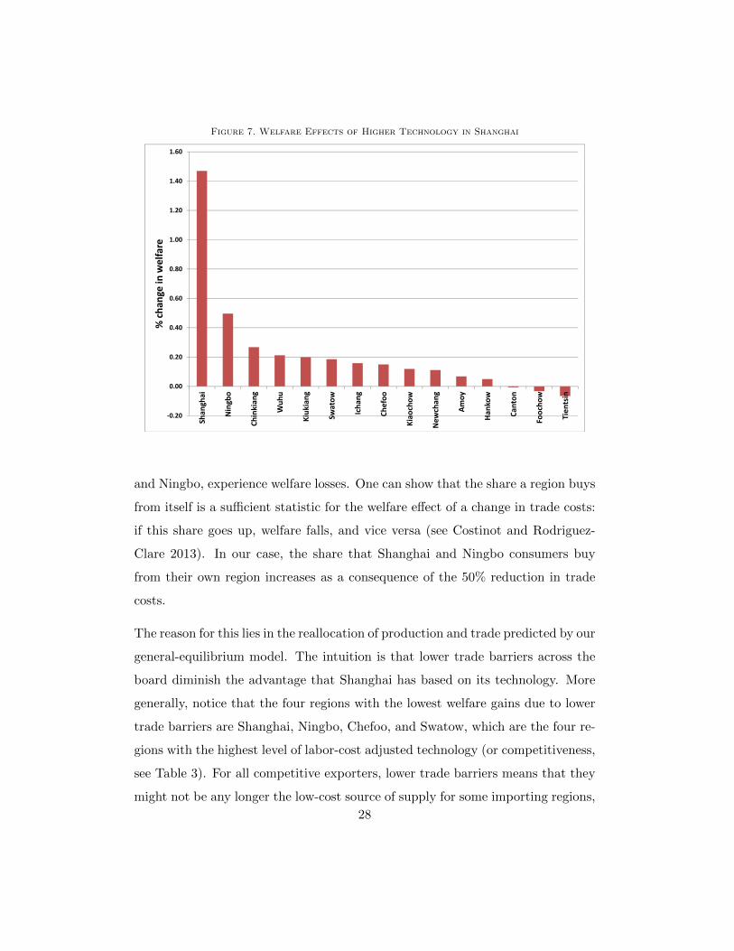
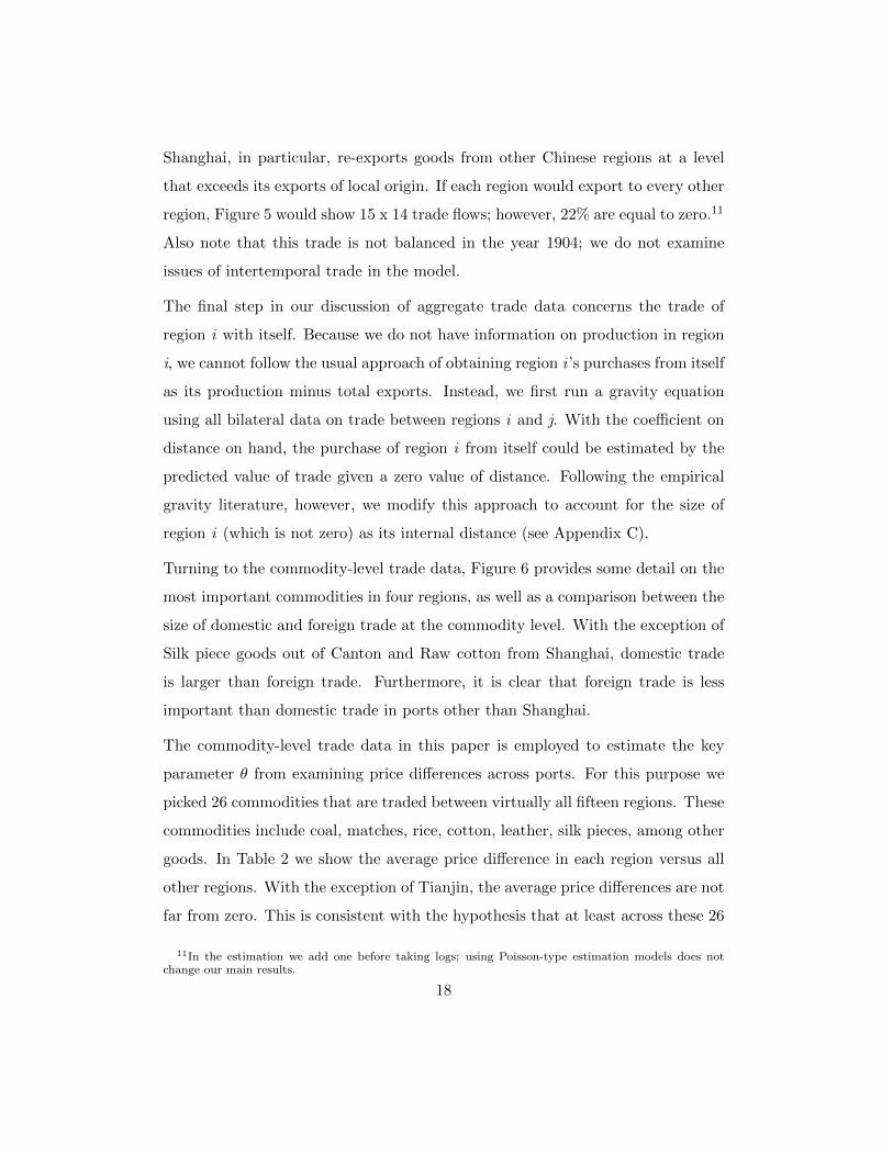
Figure 7. Welfare Effects of Higher Technology in Shanghai

0.60

0.80

1.00

1.20

1.40

1.60

% c

ha

ng

e i

n w

elf

are

-0.20

0.00

0.20

0.40

Sh

an

gh

ai

Nin

gb

o

Ch

ink

ian

g

Wu

hu

Kiu

kia

ng

Sw

ato

w

Ich

an

g

Ch

efo

o

Kia

och

ow

Ne

wch

an

g

Am

oy

Ha

nk

ow

Ca

nto

n

Fo

och

ow

Tie

nts

in

% c

ha

ng

e i

n w

elf

are

and Ningbo, experience welfare losses. One can show that the share a region buys

from itself is a sufficient statistic for the welfare effect of a change in trade costs:

if this share goes up, welfare falls, and vice versa (see Costinot and Rodriguez-

Clare 2013). In our case, the share that Shanghai and Ningbo consumers buy

from their own region increases as a consequence of the 50% reduction in trade

costs.

The reason for this lies in the reallocation of production and trade predicted by our

general-equilibrium model. The intuition is that lower trade barriers across the

board diminish the advantage that Shanghai has based on its technology. More

generally, notice that the four regions with the lowest welfare gains due to lower

trade barriers are Shanghai, Ningbo, Chefoo, and Swatow, which are the four re-

gions with the highest level of labor-cost adjusted technology (or competitiveness,

see Table 3). For all competitive exporters, lower trade barriers means that they

might not be any longer the low-cost source of supply for some importing regions,

28

Figure 8. Welfare Effects of Higher Technology in Hankow

0.60

0.80

1.00

1.20

1.40

1.60

% c

ha

ng

e i

n w

elf

are

-0.40

-0.20

0.00

0.20

0.40

Ha

nk

ow

Kiu

kia

ng

Sw

ato

w

Ich

an

g

Wu

hu

Ch

efo

o

Ch

ink

ian

g

Ne

wch

an

g

Am

oy

Kia

och

ow

Tie

nts

in

Sh

an

gh

ai

Ca

nto

n

Fo

och

ow

Nin

gb

o

% c

ha

ng

e i

n w

elf

are

relative to slightly less competitive regions that are located geographically closer.

If a competitive exporter ceases to serve a particular region, this is a movement

in the direction of autarky, and welfare falls.

The difference between the more strongly negative welfare effects in Shanghai

and Ningbo, compared to Swatow and Chefoo, can be explained by their different

geographic location. Shanghai and Ningbo are centrally located close to the

Yangzi Delta. This means that before the reduction of trade barriers, given their

high level of competitiveness they exported to many other locations, and the

reduction in trade barriers has the potential that they lose their status of low-cost

supplier in many importing regions. In contrast, Chefoo and Swatow are located

in geographically more remote parts of China, North and South, respectively.

They lose some markets as the result of the lower trade barriers, while they hold

on to others due to their geographic remoteness. As a consequence, Chefoo and

Swatow lose less than Shanghai and Ningbo.

29

In the second half of Table 6 we experiment with a more extreme reduction in

geographic barriers from the baseline to zero-gravity (setting all iceberg coeffi-

cients to virtually dni = 1). As a result, overall trade increases more than in the

previous case, although the increase remains, with 54%, relatively modest. The

distribution of welfare gains presents the same pattern as before, although with

higher magnitudes.

Table 6—Lower Geographic Barriers and Welfare

Trade barriers down 50% Trade barriers down to zero% change relative to baseline % change relative to baselineWelfare Prices Wages Welfare Prices Wages

Amoy 2.58 -7.15 -2.07 22.03 -35.69 16.35Canton 1.67 -0.03 3.24 10.18 -17.51 4.25Chefoo 0.17 4.25 9.36 5.79 -6.35 12.64

Chinkiang 0.75 -2.90 -3.53 13.68 -27.00 7.91Foochow 2.15 0.05 4.02 17.21 -21.23 13.61Hankow 2.01 10.23 10.30 2.49 6.95 8.74Ichang 8.90 -26.89 -24.80 37.89 -92.07 -31.31

Kiaochow 1.95 -6.13 -2.79 19.84 -35.08 11.90Kiukiang 3.51 -8.00 -2.26 18.98 -39.09 16.31

Newchwang 4.22 -3.48 9.96 19.79 -25.86 28.25Ningbo -31.41 15.12 -32.25 -35.40 9.79 -41.17Swatow 0.27 3.22 14.44 5.45 -7.19 17.69Tientsin 3.43 4.25 8.95 10.55 -6.54 12.51Wuhu 2.38 -4.59 1.77 15.37 -28.89 13.12

Shanghai -17.29 23.73 -7.76 -32.62 31.00 -22.50

% change in overall trade % change in overall trade13.14 54.11

Note: Notes: The table shows the results of lowering geographic barriers by 50% (first half) or to virtuallyzero (0.001 of the baseline barriers; second half) from the baseline estimated values provided in Table 5without changing states of technology (which are fixed at the estimated levels provided in Table 3). Thecomparative advantage parameter is fixed at its method-of-moments estimated value of 18.7.

V. Concluding discussion

In this paper we provide estimates of a general-equilibrium trade model for China

around the year 1900, employing a new, commodity-level dataset for fifteen major

30

treaty ports. We show that the welfare effects of internal trade depend critically

on each port’s productivity, China’s economic geography via trade costs, and the

degree of regional diversity in production.

There are two main findings. First, we find that a change in productivity for

any of the ports has ripple effects throughout China. Specifically, a 20% increase

in Shanghai’s productivity raises welfare in Shanghai by about 1.5%; because

of trade, however, welfare increases not only in Shanghai but also in other re-

gions. For example, the welfare increase at a 1,300 kilometers distance away from

Shanghai, in Swatow, is still 13% of the welfare increase due to the improvement in

technology in Shanghai. Since trade diminishes smoothly over geographic space,

whether between two treaty ports or between treaty port and hinterland, these

results suggest that the foreign opening had a sizable positive welfare effect on

large portions of China. Furthermore, because factor costs, income, and produc-

tion patterns respond endogenously, welfare in some ports can actually fall, as it

does in the relatively distant Tianjin. The endogenous reallocations of produc-

tion and trade also explain the negative welfare effects we find for some ports like

Shanghai and Ningbo when trade impediments are reduced across the board.

Second, we find evidence of relatively small regional diversity in productivity

across goods for China during the treaty port era, at least in comparison with

that found in high-income countries of the late 20th century. This provides a

rationale for the aggregate size of welfare gains from internal trade we find for

China in this historical period, since differences in productivity across goods –

comparative advantage – is the source of the gains from trade in our framework.

How confident can we be about the magnitudes of the estimated welfare effects?

Clearly, the foreign opening brought many consecutive changes in technology, not

only one, to one region, as in our counterfactual. Furthermore, trade barriers fell

unevenly across regions, and in several steps over time. In principle, assuming

we had reliable estimates of the relevant port-level changes, our counterfactual

analyses could be extended to incorporate such effects. The analysis of other

31

potential gains from openness, such as the availability of new goods, learning, and

increased innovation require a more substantial extension that is left to future

work. In summary, the high rate of development since 1978 is consistent with

China’s catch-up to her long-run trajectory, suggesting that more work on the

legacy of China’s 19th century opening will help our understanding of the sources

of economic growth.

32

REFERENCES

[1] Brandt, L., D. Ma., and T. G. Rawski (2014), “From Divergence to Conver-

gence: Reevaluating the History behind China’s Economic Boom.” Journal

of Economic Literature, 52(1): 45-123.

[2] Broadberry, S., H. Guan, and D. Li (2014), “China, Europe, and the Great

Divergence: A Study in Historical National Accounting, 980-1850”, London

School of Economics working paper, July.

[3] Cassel, P. K. (2012), Grounds of Judgment. Extraterritoriality and Imperial

Power in Nineteenth-Century China and Japan, Oxford University Press.

[4] Chang, J. (1969), Industrial Development in Pre-Communist China: A

Quantitative Analysis. Chicago: Aldine.

[5] CMC (2001a), Returns of Trade and Trade Reports, China, Imperial Mar-

itime Customs, (The Maritime Customs after 1910), Statistical Department

of the Inspectorate General of Customs, Shanghai, various years.

[6] CMC (2001b), Decennial Reports, China, Imperial Maritime Customs, (The

Maritime Customs after 1910), Vol. 1 (1882-1891), Vol. 2 (1892-1901), Vol.3

(1902-1911), and Vol. 4 (1912-1921), Statistical Department of the Inspec-

torate General of Customs, Shanghai, various years.

[7] Costinot, A., and A. Rodriguez-Clare (2013), “Trade Theory with Numbers:

Quantifying the Consequences of Globalization”, manuscript, March.

[8] Dernberger, R. F. (1975), The Role of the Foreigner in China’s Economic

Development”, in D. H. Perkins (ed.), China’s Modern Economy in Historical

Perspective (Stanford, CA: Stanford University Press.

[9] Donaldson, D. (2015), “The Railroads of the Raj”, American Economic Re-

view, forthcoming.

33

[10] Eaton, J., and S. Kortum (2002), “Technology, Geography, and Trade”,

Econometrica 70: 1741-1779.

[11] Fairbank, J. K. (1978), “The Creation of the Treaty System”, in D. Twitchett

and J. K. Fairbank (eds.), The Cambridge History of China, Vol. 10 Late

Ch’ing, 1800-1911, Part I (Cambridge: Cambridge University Press).

[12] Fajgelbaum, P., and S. Redding (2014), “External Integration, Structural

Transformation and Economic Development: Evidence from Argentina 1870-

1914”, NBER Working Paper # 20217, June.

[13] Findlay, R., and O’Rourke, K. (2007), Power and Plenty: Trade, War, and

the World Economy in the Second Millennium, Princeton University Press.

[14] Helliwell, J. and G. Verdier (2001), “Measuring internal trade distances:

A new method applied to estimate provincial border effects in Canada,”

Canadian Journal of Economics 34 (4):1024-1041.

[15] Head, Keith and Thierry Mayer (2001), “Increasing returns versus national

product differentiation as an explanation for the pattern of US-Canada

trade,” American Economic Review 91 (4):858-876.

[16] Head, K., & Mayer, T. (2002). Illusory Border Effects: Distance mismea-

surement inflates estimates of home bias in trade (Vol. 1). Paris: CEPII.w

55(1): 131-168.

[17] Hsiao, L.-L. (1974), China’s Foreign Trade Statistics, 1864-1949 (Cam-

bridge, MA: Harvard University Press.

[18] Jia, R. (2014), “The Legacies of Forced Freedom: China’s Treaty Ports”,

Review of Economics and Statistics, vol. 96, 596-608.

[19] Keller, W., B. Li, and C. H. Shiue (2013), “Shanghai’s Trade, China’s

Growth: Continuity, Recovery, and Change since the Opium Wars”, IMF

Economic Review Vol. 61(2): 336-378.

34

[20] Keller, W., B. Li, and C. H. Shiue (2012), “The evolution of domestic trade

flows when foreign trade is liberalized: Evidence from the Chinese Maritime

Customs Service”, in Institutions and Comparative Economic Development,

M. Aoki, T. Kuran, and G. Roland (eds.), Palgrave Macmillan.

[21] Keller, W., B. Li, and C. H. Shiue (2011), “China’s Foreign Trade: Perspec-

tives From the Past 150 Years”, World Economy : 853 – 892.

[22] Keller, W., and C. H. Shiue (2015), “Capital Markets and Colonial Institu-

tions in China”, paper presented at the China Economic Summer Institute

conference, Beijing, August 2015.

[23] Kose, H. (2005), “Foreign Trade, Internal Trade, and Industrialization: A

Statistical Analysis of Regional Commodity Trade Flows in China, 1914-

1931, in K. Sugihara (ed.), Japan, China, and the Growth of the International

Asian Economy, 1850 – 1949 (New York: Oxford University Press), 198-214.

[24] Kose, H. (1994), “Chinese Merchants and Chinese Inter-port Trade”, in

Japanese Industrialization and the Asian Economy, A. J. H. Latham and

H. Kawakatsu (eds.), New York: Routledge.

[25] Liu, Ta-Chung, and Kung-Chia Yeh (1965), The Economy of the Chinese

Mainland: National Income and Economic Development, 1933-1959, Prince-

ton, New Jersey: Princeton University Press.

[26] Lyons, T. (2003), China Maritime Customs and China’s Trade Statistics,

1859-1948, Willow Creek Publisher.

[27] Mitchener, K. J., and S. Yan (2014), “Globalization, trade, and wages: What

does history tell us about China?”, International Economic Review 55(1):

131-168.

[28] Morse H. (1926), The Chronicles of the East India Trading Company, 1634-

1834, Vols 1-5, Oxford: Clarendon Press.

35

[29] O’Rourke, K., J. Williamson (1999), Globalization and History. The Evolu-

tion of a Nineteenth-Century Atlantic Economy, MIT Press.

[30] O’Rourke, K., J. Williamson (1994), “Late 19th Century Anglo-American

Factor Price Convergence: Were Heckscher and Ohlin Right?”, Journal of

Economic History 54: 892-916.

[31] Perkins, D. H. (1969), Agricultural Development in China 1368-1968, Aldine.

[32] Redding, S. and A. Venables (2000), “Economic geography and inequality,”

mimeo London School of Economics.

[33] Richardson, P. (1999), Economic Change in China, c. 1800-1950. Cambridge

University Press.

[34] So, B. K. L., and R. H. Myers, eds., (2011), The Treaty Port Economy in

Modern China: Empirical Studies of Institutional Change and Economic Per-

formance, China Research Monograph 65, Institute for East Asian Studies,

University of California, Berkeley.

[35] Tinbergen, J. (1962), Shaping the World Economy: Suggestions for an In-

ternational Economic Policy. New York: Twentieth Century Fund.

[36] Wei, S. J. (1996), “Intra-national versus international trade: How stubborn

are nations in global integration?” National Bureau of Economic Research

Working Paper no. 5531.

[37] Wolf, H. (1997), “Patterns of intra- and inter-state trade.” National Bureau

of Economic Research Working Paper no. 5939.

[38] Wolf, H. (2000), “Intranational home bias in trade,” Review of Economics

and Statistics 824 (4): 555-563.

36

Appendix A: Wage Data

Wages are obtained as a mean residual, by port, from an OLS regression on oc-

cupation fixed effects, year fixed effects, length of work time fixed effects (hour,

month, year), currency fixed effects. The wage for Hankow and Foochow is es-

timated as the prediction from a regression of observed wages on latitude and

longitude. The following Table A1 shows the different occupations that are avail-

able from the Decennial Reports.

Table A1—Wage Data from the Decennial Reports

Region Obs. Occupation Obs.Amoy 1 General, skilled (e.g. mechanic) 21

Canton 29 General, unskilled 19Chefoo 30 Carpenter 62

Chinkiang 91 Stonemason 57Foochow n/a Painter 4Hankow n/a Blacksmith 34Ichang 15 Coolie 19

Kiaochow 12 General, manual 24Kiukiang 8 Servant 23

Newchwang 2 Cotton/silk weaver 9Ningpo 8 Matchmaker 1Swatow 10 Tailor 26

Shanghai 12 Farmhand 4Tientsin 69Wuhu 7Total 294

Note: Notes: Data from CMC (2001b), Decennial Reports, various volumes; number of observations for1901-1911: n = 56, 1912-1921: n = 105, and 1922-1931: n = 144.

Appendix B: Labor force and gross product data

To obtain figures for the labor force of each region, we employ the average of

the population estimates of the Decennial Reports (CMC 2001b) for 1901 and

1911; there are separate estimates for the Chinese and the foreign population,

which we add together. We apply Liu and Yeh’s estimate of national labor force

37

participation in 1933 of 51.8% to obtain regional labor forces, Li (Liu and Yeh

1965, p. 182). The wage estimates from Appendix A times these labor forces

yield a region’s wage income, wiLi.

Recall that our regions are defined on the basis of the customs districts of the

treaty ports. While the ports were of central importance, it would be an over-

statement to treat the customs districts as exclusively urban areas. In order to

capture the large contribution of agriculture to China’s gross product at this time,

we estimate the gross product of each region by augmenting the wage income wiLi

with an estimate of the region’s agricultural production, based on Perkins (1969).

The value of agricultural production in each province is estimated for the years

1914-1918 from data on acreage for barley, corn, cotton, fiber (including jute,

hemp, ramie, and flax), millet, peanuts, rice, sesame, sorghum, soybeans, sug-

arcane, tobacco, and wheat (Perkins 1969, Appendix C); yield data for these

crops, see Perkins 1969, Appendix D, and crop prices given in Perkins (1969,

Table D.31). Given the value of agricultural production in each province, piQi,

we estimate each regioni’s agricultural production, piQi, as piQi = si × ppQp ,

where si is the fraction of region i’s population of the population in the province

in which region i is located. The gross product of region i, Yi = wiLi +λ× piQi ,

with λ = 1.1 in the baseline analysis. We have confirmed that our main findings

are not sensitive to choosing other reasonable values for λ (results available upon

request).

Appendix C: Purchases-from-self

The expenditures of region i on production of i are not observed. We there-

fore estimate a gravity equation regression of bilateral trade flows on a set of

standard gravity covariates to predict the value of each port’s consumption of its

own goods. These covariates include bilateral distance, the origin and destination

ports’ respective population sizes, and a dummy variable indicating the destina-

tion port’s location on the Yangtze River. Values for each of these variables are

38

for 1904; however, estimates are also produced including additionally data for the

years 1895 through 1899. For these estimates which employ multiple years’ worth

of data, a time fixed effect is included. To preserve zero trade flows and maintain

a sufficiently high sample size after taking logarithms, each trade flow value is

increased by one.

Several flexible versions of the gravity equation are employed, including the stan-

dard log-linear gravity equation, a Poisson pseudo-maximum likelihood (PPML)

estimator of the gravity relationship, and a PPML estimator possessing squared

and cubed logarithms of distance. Because of the out-of-sample nature of the

predictions, the preferred specifications are ones that are able to most closely fit

the relation between bilateral trade flows and distance between ports, i.e., those

specifications for which the (joint) significance of the coefficient(s) on distance is

suitably high. Finally, each specification is either estimated by pooling the data

across all 15 ports, or individually for each port. To capture a realistic measure

of internal distance within treaty ports dii, five alternative measures of internal

distance from the literature are used for the predictions for purchases-from-self.

These include (with dij denoting the distance between ports i and j):

1) Wei (1996): dii = 0.25 minjdij ,

2) Wolf (1997, 2000): dii = 0.50 mean (dij),

3) Redding and Venables (2000): dii = 0.33√areai/π ,

4) Head and Mayer (2000): dii = 0.67√areai/π,

5) Helliwell and Verdier (2001): dii = 0.52√areai ,

where areai denotes the area of the prefecture in which the treaty port i is located.

In total, the various specifications and internal distance measures generate 2 x 3

x 2 x 5 = 60 candidate estimates for purchases-from-self for each of the 15 treaty

ports. The preferred estimates are chosen along three dimensions. First, by com-

paring the correlation between predicted bilateral trade flows xij and observed

39

trade flows xij . Estimates with a high correlation do a relatively good job of pre-

dicting actual purchases from other ports. For the second and third dimensions,

two empirical regularities are exploited: the fact that modern large economies

(which in turn tend to be larger exporters) generally have larger magnitudes of

consumption of their own goods than smaller economies in absolute terms, and

that the ratio of exports to purchases-from-self tends to run from around 0.10

for smaller, isolated countries like Australia, to around 0.25 for the U.S., to 0.35

for large countries such as Germany with many close, large trading partners. We

therefore consider as the second dimension the correlation between total trade,∑j xij , and predicted self-purchases xii, and the third dimension as the ratio of

total trade to predicted purchases-from-self,∑

j xij/xii. Estimates that perform

well in the second and third dimensions, by having, respectively, a high correlation

and a “reasonable” ratio, perform comparatively well in predicting the relative

magnitude of trade-with-self.

Of the 60 estimates for purchases-from-self, the four best candidate estimates

are chosen upon evincing a high degree of performance in each dimension and

after fitting the distance variable(s) well: when pooling the data across all ports,

they are: i) PPML with a cubic expansion of log distance using Wolf’s (1994)

internal distance and data for 1904, ii) PPML of standard gravity using Helliwell

and Verdier’s (2001) internal distance and data for all six years, iii) PPML of

standard gravity using Head and Mayer’s (2001) internal distance and data for

1904, and with port-level regressions, iv) PPML of standard gravity using Wolf’s

(1994) distance and data for 1904.

40