FOREIGN EXCHANGE RATE EXPOSURE OF AUTOMOTIVE...
57
FOREIGN EXCHANGE RATE EXPOSURE OF AUTOMOTIVE MAKERS: CASE STUDY Authors Peng Liu Yuanyuan Zhao Advisor Göran Anderson Master Thesis Autumn 2009
Transcript of FOREIGN EXCHANGE RATE EXPOSURE OF AUTOMOTIVE...
FOREIGN EXCHANGE RATE EXPOSURE OF AUTOMOTIVE MAKERS: CASE
STUDY
Authors Peng Liu Yuanyuan Zhao
Advisor Göran Anderson
Master Thesis Autumn 2009

2
Abstract Title: Foreign Exchange Rate Exposure of Automotive Makers:
Case Study Seminar Data: 2010-01-15 Course: FEKP01, Master Thesis in Finance, 10 Swedish Credit (15
ECTS) Authors: Peng Liu and Yuanyuan Zhao Advisors: Göran Anderson Key words: Stock price, exchange rate, Stock market index, Spillover
model, GARCH Model Purpose: The aim of our paper is to find out the relationship between
exchange rate and corporate value. We are going to study the impact of volatility of exchange rate on automakers’ value.
Theoretical perspective: The theoretical framework mainly involves prior research in the area of exchange rate exposure and corporate value. Further, the relationship between corporate performance and market performance is studied.
Methodology: Colleting data for four largest automakers in the world as
well as exchange rate and stock market index to run regression to study their relation ship. Unconditional Spillover model is used.
Results: Five out of nine exchange rates we selected are significant
for corporate stock price but weakly impact on corporate stock price.
Conclusion: The impact of foreign exchange rate on corporate stock
price is weak or insignificant.
3
Table of Contents ABSTRACT ............................................................................................................................................2
1. INTRODUCTION..........................................................................................................................5
1.1 BACKGROUND .....................................................................................................................5 1.2 DISCUSSION OF PROBLEM ................................................................................................8 1.3 PURPOSE................................................................................................................................9 1.4 DELIMITATIONS ...................................................................................................................9 1.5 OUTLINE OF THE THESIS .................................................................................................10
2. THEORY ...................................................................................................................................... 11
2.1. LITERATURE REVIEW....................................................................................................... 11 2.2. CHANGE OF FOREIGN EXCHANGE RATE ...................................................................................14 2.3. MOTIVATIONS OF STUDY ON FOREIGN EXCHANGE RATE EXPOSURE..................16 2.4. EXCHANG RATE EXPOSURES..........................................................................................17
2.4.1. Accounting exposure......................................................................................................17 2.4.2. Transaction exposure.....................................................................................................18 2.4.3. Economic exposure........................................................................................................18
3. METHODOLOGY AND DATA..................................................................................................20
3.1. RESEARCH APPROACH.....................................................................................................20 3.2. DATA COLLECTION .................................................................................................................20
3.2.1. Sources of information...................................................................................................20 3.2.2. Sample ...........................................................................................................................21 3.2.3. Data description ............................................................................................................23 3.2.4. Excluded Observations..................................................................................................24
3.3. METHODOLOGY......................................................................................................................24 3.3.1. Related Models ..............................................................................................................24 3.3.2. The employed model ......................................................................................................26 3.3.3. Tests ...............................................................................................................................29 3.3.4. Hypotheses.....................................................................................................................30
3.4. VALIDITY AND RELIABILITY ...................................................................................................31 3.4.1. Validity...........................................................................................................................31 3.4.2. Reliability ......................................................................................................................32
4. EMPIRICAL FINDINGS ............................................................................................................33
4.1. DESCRIPTIVE STATISTICS................................................................................................33 4.1.1. Toyota ............................................................................................................................36 4.1.2. General Motors .............................................................................................................38 4.1.3. Volkswagen ....................................................................................................................40 4.1.4. Ford ...............................................................................................................................41
4.2. RESULTS OF TESTS............................................................................................................43 4.2.1. Heteroscedasticity .........................................................................................................43 4.2.2. Variables omitting..........................................................................................................44

4
5. ANALYSIS....................................................................................................................................47
5.1. EFFECT OF EXCHANGE RATE ON CORPORATE STOCK PRICE .................................47 5.2. EFFECT OF MARKET INDEX ON CORPORATE STOCK PRICE ....................................49 5.3. HYPOTHESES......................................................................................................................51
6. CONCLUSION.............................................................................................................................53
REFERENCE .......................................................................................................................................55
5
1. INTRODUCTION
In the first chapter of this paper, we introduce the whole picture of this subject to
readers. Background, problem specification, purpose and research delimitation are
presented. This chapter is ended by a disposition of the thesis.
1.1 BACKGROUND
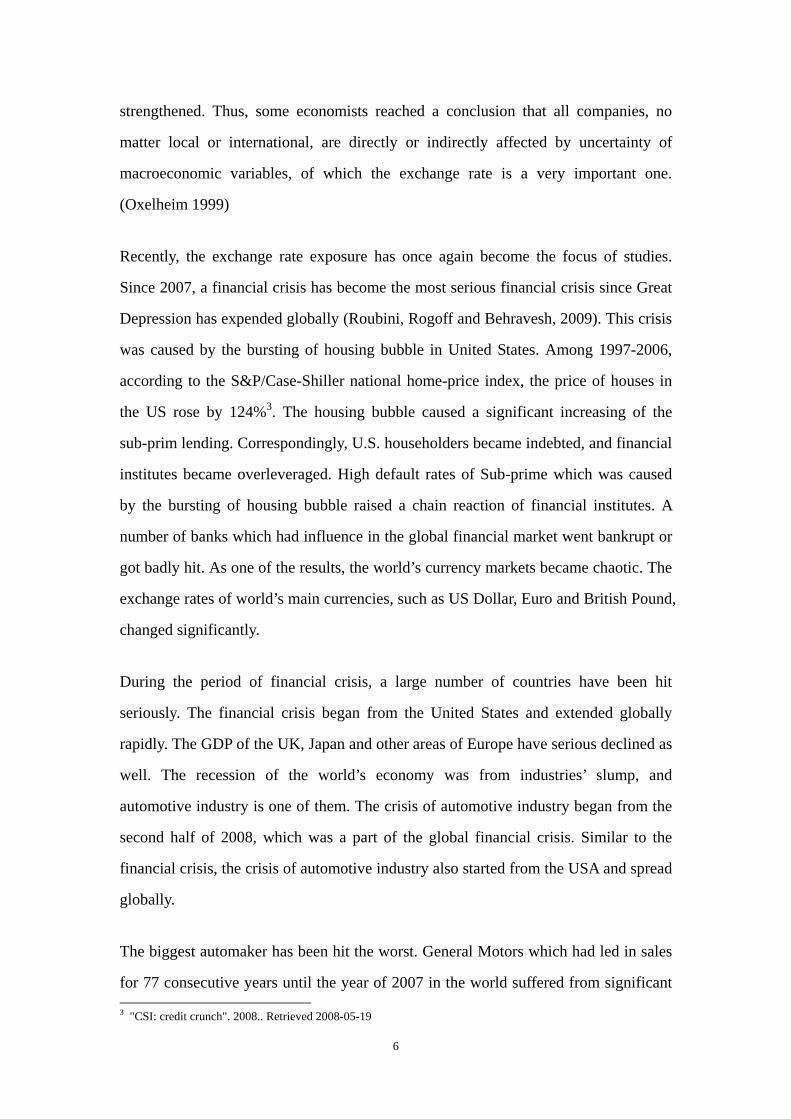
After the collapse of Bretton Woods System1 in 1970’s, many countries have
implemented floating exchange rates. Simultaneously, uncertainties of the exchange
rates have become one of the major risks for enterprises, especially for those
multinational corporations. Exchange rate risk has been firstly paid attention by
financial industry, because many financial institutes, which are involved in trading
and loaning of foreign currencies, have been affected by the floating of exchange rate.
With the expansion of global business, researchers realized that non-financial firms
would be affected by the uncertainty of foreign exchange rate as well. People found
out that the value of firm, which was involved in foreign currencies and based on
activities such as selling or producing abroad, is influenced by the foreign exchange
rate. In the real world, the impacts of floating exchange rate have been clearly
illustrated. In the late of 1990s, Asian Financial Crisis2 started from the collapse of
Thai baht which was caused by freely floating of Thai baht against US dollar. Those
mostly affected countries had suffered from the worst slumping of GNPs and the
highest depreciation of domestic currencies. The issue of exchange rate has become
the focus of economists and researchers. As long as globalization has been intensified,
the influence of exchange rate among various economies has been gradually
1 The system was built by most of the world’s leading nations at Bretton Woods, New Hampshire, in 1944. It agreed that US dollar can be convertible into gold at $35 per ounce and other currencies should fixed exchange rates against US dollar. 2 Asian Financial Crisis was a regional financial crisis beginning in July 1997 and gripped much countries of Asia. Indonesia, South Korea and Thailand were the countries most affected.
6
strengthened. Thus, some economists reached a conclusion that all companies, no
matter local or international, are directly or indirectly affected by uncertainty of
macroeconomic variables, of which the exchange rate is a very important one.
(Oxelheim 1999)
Recently, the exchange rate exposure has once again become the focus of studies.
Since 2007, a financial crisis has become the most serious financial crisis since Great
Depression has expended globally (Roubini, Rogoff and Behravesh, 2009). This crisis
was caused by the bursting of housing bubble in United States. Among 1997-2006,
according to the S&P/Case-Shiller national home-price index, the price of houses in
the US rose by 124%3. The housing bubble caused a significant increasing of the
sub-prim lending. Correspondingly, U.S. householders became indebted, and financial
institutes became overleveraged. High default rates of Sub-prime which was caused
by the bursting of housing bubble raised a chain reaction of financial institutes. A
number of banks which had influence in the global financial market went bankrupt or
got badly hit. As one of the results, the world’s currency markets became chaotic. The
exchange rates of world’s main currencies, such as US Dollar, Euro and British Pound,
changed significantly.
During the period of financial crisis, a large number of countries have been hit
seriously. The financial crisis began from the United States and extended globally
rapidly. The GDP of the UK, Japan and other areas of Europe have serious declined as
well. The recession of the world’s economy was from industries’ slump, and
automotive industry is one of them. The crisis of automotive industry began from the
second half of 2008, which was a part of the global financial crisis. Similar to the
financial crisis, the crisis of automotive industry also started from the USA and spread
globally.
The biggest automaker has been hit the worst. General Motors which had led in sales
for 77 consecutive years until the year of 2007 in the world suffered from significant 3 "CSI: credit crunch". 2008.. Retrieved 2008-05-19
7
decline in sales and it had to face a hedge problem. Compared to the year of 2007,
GM’s total sales went down 11 percent in 2008. Especially during the third and the
fourth quarters, the sales went down 11.4% and 26% respectively, compared with the
same quarter a year ago4. On July 10, 2009, General Motors Corporation was
reorganized to be General Motors Company with brands, workforces and plants
spanned-off. The other two of “big three”5 automakers in the United States were also
suffered from the crisis, and they were force to seek fund aiming to get out of the
dilemma. As the second largest automaker in the U.S. and the fourth largest in the
world, Ford Motor also had to face a difficult situation. From 2005 to 2008, its
revenue went down 17.4% and profit was even down 78.09%6. In order to tide over
the difficulties, Ford is spinning-off brands to obtain a better finance situation. (See
Table 1)
After the reorganization of General Motors, Toyota which is based in Japan has placed
the first in sales among automotive manufactures in the world. However, it has not
escaped from the impact of the crisis. On December 22, 2008, Toyota announced their
expected loss for the first time in the latest 70 years in its core vehicle-making
business. A $1.7 billion loss, which is related to group operating revenue, has been its
first time since 1938.
The situation in Europe is not so bad as the United States and Japan. Although Saab
(Sweden), Volvo Cars (Sweden) and Opel (Germany) have been spinning-off from
General Motors and Ford, they were not influenced significantly. Let us take
Volkswagen which is the largest automaker in Europe and the third largest in the
world as an example. From Year 2005 to 2008, when other leader auto manufactures
were suffering from significant decline, the annual sales of Volkswagen had increased
10.08%, 3.8% and 4.5% and the corresponding profit increased 74.46%, 3.8% and
4 Data comes from the official website of GM. 5 General Motors, Ford and Chrysler are called “big three” automakers in the United States. 6 Data comes from “DataStream”.
8
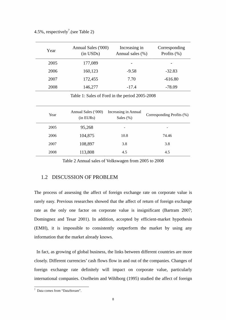
4.5%, respectively7.(see Table 2)
Year Annual Sales ('000)(in USDs)
Increasing in Annual sales (%)
Corresponding Profits (%)
2005 177,089 - -
2006 160,123 -9.58 -32.83
2007 172,455 7.70 -616.80
2008 146,277 -17.4 -78.09
Table 1: Sales of Ford in the period 2005-2008
Year Annual Sales (‘000)(in EURs)
Increasing in Annual Sales (%) Corresponding Profits (%)
2005 95,268 - -
2006 104,875 10.8 74.46
2007 108,897 3.8 3.8
2008 113,808 4.5 4.5
Table 2 Annual sales of Volkswagen from 2005 to 2008
1.2 DISCUSSION OF PROBLEM
The process of assessing the affect of foreign exchange rate on corporate value is
rarely easy. Previous researches showed that the affect of return of foreign exchange
rate as the only one factor on corporate value is insignificant (Bartram 2007;
Domingnez and Tesar 2001). In addition, accepted by efficient-market hypothesis
(EMH), it is impossible to consistently outperform the market by using any
information that the market already knows.
In fact, as growing of global business, the links between different countries are more
closely. Different currencies’ cash flows flow in and out of the companies. Changes of
foreign exchange rate definitely will impact on corporate value, particularly
international companies. Oxelheim and Wihlborg (1995) studied the affect of foreign
7 Data comes from “DataStream”.

9
exchange rate on corporate value with other macroeconomic factors. And, they
concluded that foreign exchange rate is affecting corporate value.
The problem we want to solve in this paper is how to measure the exposure of foreign
exchange rate on corporate value. Since study the return of exchange rate as the only
factor affecting on corporate is insignificant, why do not we try the volatility? In
addition, reference to the research of Oxelheim and Wihlborg, exchange rates of
different corporate operational aspects could also be significant variables for
corporate value.
1.3 PURPOSE
Through the financial crisis, we notice that the exchange rate changes dramatically,
and it does have impact in people’s daily life. Thus, we think it might as well have
some kind of influence on corporate value. Thus, we are very interested in studying
whether the exchange rate could influence corporate value and how much it can be.
The purpose of this thesis is to empirically test the relationship between exchange rate
and corporate value, mainly the exchange rate exposure on automakers’ value.
1.4 DELIMITATIONS
In this paper we do not try to investigate hedging and derivative activity on risk
management of foreign exchange rate. Furthermore, corporate operating strategy,
product structure and market operation are not studied in this paper.
In addition, the impact of exchange rate on corporate value under financial crisis is
not studied in this paper. Because during financial crisis period, both exchange rate
and corporate performance are unstable. There are too many factors that would
influence these two variables above, and those are too complex for us to study. The
most important reason for not considering financial crisis is that, during the period of
crisis, changes of corporate value and exchange rate could not be represented as the
10
typical relationship between them.
1.5 OUTLINE OF THE THESIS
The outline of this paper is as follow.
In Chapter 1, we introduce the whole picture of this subject to readers. Background,
problem specification, purpose and research delimitation are presented. This chapter
is ended by a disposition of the thesis.
In Chapter 2, we firstly present previous literatures on the subject including models
and results. Furthermore, this chapter includes specific introduction of three different
kinds of exchange rate exposures.
In Chapter 3, we present the way how the data are collected and the methodology
used in our research. Some sample information and different empirical models related
to this research are presented as well. Further, we describe data processing and
reliability and validity of this study.
In Chapter 4, we present obtained result of regression to readers. Starting with
description of variables and data, requirements of assumption are also presented.
Specification of Empirical result and regression tests is the main content of this
chapter.
In Chapter 5, we analyze different variables’ effect on corporate stock price. The
variables are divided to two groups as exchange rate and market index to analyze. The
hypotheses are also discussed in this chapter.
In Chapter 6, a short conclusion is presented with possible improvements for the
research in this field.
11
2. THEORY
In the chapter of theory, we firstly present previous literatures on the subject including
models and results. Furthermore, this chapter includes specific introduction of three
different kinds of exchange rate exposures.
In this paper, we select the stock prices of Toyota, General Motors, Volkswagen and
Ford as dependent variables and make regression for each one with the corresponding
foreign exchange rates and stock market index as independent variables. We raised
four hypotheses which are described in chapter 3 in this paper to test the influence of
market index and exchange rates of main market, the areas where main competitors
and main suppliers are based in and the area of main production on corporate value.
For study the value of corporation, cash flow is the best indicator (Koller, Goedhart
and Wessels, 1990). Based on the corporate finance theory, the corporate value is
calculated by the future cash flow. Therefore, the study of the relationship between
corporate cash flow and foreign exchange rate will well indicate the exchange rate
exposure on corporate value. However, the data of cash flow is not readily available.
In some extent, operation cash flow is confidential and the data are rarely published in
the annual report. Since the yearly data is not frequent enough, we use stock price as
the proxy of corporate value in this paper. Accurately, stock price is the measure of
equity value which is a part of corporate value. As many articles did, we use stock
price to indicate corporate value in this paper.
2.1. LITERATURE REVIEW
A large number of articles are written for the analysis of exchange rate exposure on
non-financial corporate value. There are two main types of approach. One is making
12
regression to study the relationship between basis stock prices and foreign exchange
rate. Adler and Dumas (1984) were the first fining exchange rate exposure as the
impact of unanticipated changes in exchange rates on stock prices, and raised the
theory that exchange risk can be quantified by the regression coefficients which
regressed from stock price returns against foreign exchange rate changes. The other is
measuring currencies’ exposure on individual corporate cash flow. Most empirical
literatures focus on equity prices primarily, since cash flow data is not readily
available. Instead, stock prices are used as a proxy for cash flows (Bartram 2006).
The research of stock prices is usually to analysis the response of a big group of
companies in different economies and industries to shocks of foreign exchange rate.
The cross economies and industries studies of a big group of samples generally
choose trade weighted index8 as the indicator of exchange rate. Jorion (1990) was the
first using a regression of stock returns of 287 US multinational firms on changes in
foreign exchange rate index to get a result where only few firms have significant
exchange rate exposure. Ki-ho Kim (2002) analyzed monthly data of the S&P’s 500
composite stock price index for the 1970-1998 and found that the index is related to
the industrial production positively, whereas it is negatively to the real exchange rate.
Griffin and Stulz (2001) studied weekly stock return data on 320 industry pairs in six
countries from 1975 to 1997. They found that common shocks to industries across
countries are more important than competitive shocks. Correspondingly, Blenman,
Lee and Walker (2006) used three models of foreign exchange rate exposure to
investigate the significance of exposure for US multinationals during the period of
1985-1997. They found that exchange exposure is related to firm size negatively,
whereas it is positively related to the degree of foreign operation.
Some literatures study on the relationship between the changes of stock price returns
and the foreign exchange rate changes of particular economy or industry. In these
articles, authors usually choose one or several specific foreign exchange rates which 8 Trade weighted index is a weighted average of exchange rates of home and foreign currencies, with the weight for each foreign country equal to its share in trade.
13
are closely related to the studied economy and industry. Yaqiong Pan (2009) chose
iron and steel industry’s panel data of the period 2005-2008 of the companies listed on
the Shanghai and Shenzhen Stock Exchange. He built the augmented Jorion Model to
analyze the sensitivity of stock price returns to exchange rate changes and found that
Chinese iron and steel industry has significant exposure to USD and JPY and
insignificant exposure to EUR and HKD. Hieh, Lin and Wang (2008) studied the
effect of exchange rate of NT dollar against US dollar on the corporate values of food,
glass, electricity, paper, rubber and steel industries. They found that if the discount
rate is large enough, the exchange rate uncertainty is positively related to the
corporate value. Bahmani-Oskooee and Hegerty (2007) analyzed disaggregated
export and import data for 117 Japanese industries of the period 1973-2006. They
found that the trade shares of most industries are relatively unaffected by uncertainty
of Yen-Dollar exchange rate in the long run while some industries are influenced by
exchange-rate volatility in the short run, but this effect is often ambiguous.
Bahamani-Oskooee and Wang (2009) disaggregated the annual trade data between
Australia and the USA for 108 commodities over the period of 1962-2005, and got the
result that in the long run both the export and import industries are sensitive to the real
exchange rate of Australia Dollar-US Dollar.
In contrast, the studies of foreign exchange rate exposure on corporate cash flow
always focus on individual companies. In this way, researchers can consider more
factors such as sales, production and competition than simply study exchange rate of
home currency against one foreign currency. Choi (1986) introduced a model to study
the effect of exchange rate uncertainty on corporate value, which considers the input
and output elasticity of foreign exchange rate. From management’s point of view,
considering the factors of sales, production and competition, Oxelheim and Wihlborg
(1995) used quarterly data to measure Volvo car’s cash flow exposure to exchange
rates and other macroeconomic variables.
14
2.2. Change of foreign exchange rate
Foreign exchange rates started to float freely since 1971 after the collapse of Bretton
Woods System. When Bretton Woods system held, members of the system were
required to establish a parity of their national currencies in terms of gold and to
maintain exchange rates within plus or minus 1% of the parity by intervening in their
foreign exchange markets. In the other word, the change of exchange rates among the
members’ currencies was limited in 1% under Bretton Woods System. From 60’s to
70’s, there were several breakouts of U.S. Dollar crisis. In Dec 1971, "Smithsonian
Agreement" was signed for the marked depreciation of dollar against gold, while the
U.S. Federal Reserve Bank refused to sell gold to foreign central banks, bringing the
U.S. dollar and gold linked system in name only. In Feb 1973, associated with further
depreciation of U.S. Dollar, the world’s major currencies were forced to implement a
floating exchange rate system due to the impact of speculators. In addition, "Jamaica
Agreement" was signed in 1976, which provides the legalization of the floating
exchange rate and non-monetary of gold, bringing the total collapse of the Bretton
Woods system. From that time on, the world has entered a period of floating exchange
rates.
However, the research of exchange rate changes is worthless if the global market is
perfect9. In the perfect market, there are no custom duty cost and transaction cost.
When the exchange rate causes a different price of a product between two regions or
two countries, goods and money can move freely between regions and countries and
finally get equilibrium. We pick the changes of exchange rate between China and the
USA as an example and set SC as exchange rate of Chinese Yuan and SA as exchange
rate of US dollar. We chose a product which exists in both China and the USA, and its
price is PC and PA in China and the USA respectively. At the equilibrium condition, the
ratio of exchange rates SC/SA is equal to 5 and the ration of prices PC/PA is equal to 0.2.
In case Chinese Yuan depreciates and SC/SA become to 10, the real price of this 9 In this paper, the perfect market means that there is no transfer cost of goods and money between countries, such as customs duty, transportation cost and agency cost.
15
product will be doubled in the USA compared with China. Without any transfer cost,
the product will be rushed into the USA form China. The increased supply of the
product in the USA will decrease the price and the increased demand of the product in
China will increase the price until the real prices between China and the USA become
equal again.
In the other case, the price index IA of the USA increased, which means that the
consumption in the USA is higher than it in China. The fund will be rushed into China
from the USA to consume and invest. As the result, the demand of Chinese Yuan will
increase and lead SC increases until the real price index IC of China become as high as
IA. We can find that under the perfect market, the condition will keep in equilibrium
of A B A
B A C
S P I= =S P I
in the long term. While the real world is imperfect and we will
discuss the impact of exchange rate in the real world below.
At the macro level, changes of exchange rate do not work so much on firms’ value if
the market is perfect. While, at micro level, the changes of exchange rate will not
affect firms’ value if it could totally “Pass through” to customers. These cases are
particularly in monopoly market or the market of low price elastic products. In these
markets, increase of price will not impact the dem and of products. Firms which suffer
from increased price of input due to changes of exchange rate could increase the
products price to compensate the higher cost and do not need to be worried about
demand decreasing. In perfect competition market, increased input price can not
totally “pass through” to customers because the demand of products decreases as price
increases. Meanwhile, decreased demand of products causes decrease of input and
decreased demand of input causes price input decreasing. This process leads to a new
equilibrium point where firms could maintain the net cash flow level with proper cost
of input and proper price of products.

16
2.3. MOTIVATIONS OF STUDY ON FOREIGN EXCHANGE RATE
EXPOSURE
In the real world, the market is not perfect. The volatility of exchange rates could not
get an equilibrium point from free transaction of funds and products (Oxelheim, 1999).
The imperfect of the market, such as customs duty, transportation cost and agency
cost, leads to value10 gaps among countries. And, the value gaps always impact
international trade. Two opposing views were proposed by economists. De Grauwe
(1988) believes that since the beginning of floating exchange rates the international
trade has declined by more than a half. Hooper and Kohlhagen (1978) found a
negative relationship between the volatility of exchange rate and international trade
volume. While, other economists argued that the volatility of exchange rate could
stimulate the growth of international trade. (Gotur, 1985)
It is believed that foreign exchange rates are strongly linked to the profitability and
financial decision of firms (Oxelheim, 1999). One of the central motivations for the
creation of the euro was to eliminate exchange rate risk to enable European firms to
operate free from the uncertainties of changes in relative prices resulting from
exchange rate movements (Domingnez and Tesar, 2004). The volatility of foreign
exchange rates could impact corporate cash flows. Particularly for the firms with
foreign-currency based activities, such as exporters and importers (Bartram, 2007).
Importing firms can benefit from the appreciation of local currency since they could
afford more products from foreign market. Vice versa, local products subsequently
become more affordable to foreign consumers since depreciation of local currency
and thus exporting firms can benefit from it.
Recently, there is a new theory that any firms no matter domestic or international can
be affected by changes of exchange rate (Oxelheim, 1999). For example, there is an
automaker which only produces and sells cars in the USA. Although it does not have
10 The “value” here refers to the value of products, contracts, bonds, futures and so on.

17
any overseas business, it is still affected by exchange rate changes of US dollar. We
assume that this automaker is called Localcars. Localcars’s cash flow can not be
affected by changes of exchange rate directly because of Localized procurement and
sales. However, there are several situations in that exchange rate changes of US dollar
will also impact Localcars’s cash flow indirectly. First, the supplier of Localcars may
be a foreign-related company which is affected by the change of US dollar’s exchange
rate and thus localcars’s cost would be affected because of the change of inputs’ price.
Second, the competitor of Localcars may be a foreign-related company such as Toyota.
Products’ price of Toyota decreases in the USA when US dollar appreciates and thus
products’ competitiveness and demand of Localars would be decreased. Third, price
of gasoline in the USA will definitely be affected by changes of US dollar’s exchange
rate, and cost of driving (cost of gasoline) is an important factor of vehicle demand.
Depreciation of US dollar leads appreciation of gasoline price and thus the demand of
Localcars’s products would be decreased. Sometimes, these three situations exist and
to play a role together. In the first situation Localcars’s inflow of cash is affected and
in the second and third situation its outflow of cash is affected. The volatility of cash
flow leads unstable corporate value and thus the volatility of exchange rate can affect
every firm’s value.
2.4. EXCHANG RATE EXPOSURES
The quantitative influence of exchange rate is called as exchange rate exposure. There
are three exposures of exchange rate, accounting exposure, transaction exposure and
economic exposure.
2.4.1. Accounting exposure
Translation exposure is the possibility of foreign currencies’ fund changes in firm’s
balance sheet due to the changes of foreign exchange rate. It is not actual loss (or gain)
but a loss (or gain) of book, and will influence the result of financial report. It is
illustrated by the example below that this description is too abstract to understand.
18
There is a company based in China needs to import equipments from the USA. We
assume the total cost of the equipments is 500 thousand US dollar. At the time when
import contract was singed the exchange rate of Chinese Yuan against US dollar is 8/1.
The equipments cost 4 million Chinese Yuan and the liability was recorded in the
company’s balance sheet. In the end of accounting period, the exchange rate of
Chinese Yuan against US dollar changed from 8/1 to 7/1, at the time the total cost of
the equipments is 3.5 million Chinese Yuan. The gain of 0.5 million Yuan in the
companies balance sheet caused by exchange rate change is translation exposure.
2.4.2. Transaction exposure
Transaction exposure is actual loss (or gain) for companies whose payables and
receivables are denominated in foreign currencies due to change of foreign exchange
rate. The same as accounting exposure, we use an example to illustrate the abstract
description.
The same Chinese company we used in the previous section’s example needs import
some other equipments from Europe. We assume the total cost of the equipment is 1
million Euros. In this transaction, the company signed a contract with a European
company first and pay for the equipments three months later. The exchange rate of
Chinese Yuan against Euro was 9/1 when the contract was signed. The equipments
cost 9 million Chinese Yuan at that time. Three months later, the exchange rate of
Chinese Yuan against Euro changed to 10/1 at the time of the Chinese company paid
for the equipments. In this exchange rate, the Chinese company has to pay the
European company 10 million Yuan. The lost of 1 million Yuan of the Chinese
company is transaction exposure.
2.4.3. Economic exposure
Economic exposure is a possibility of benefit change in a specific future period due to
the change of foreign exchange rates. In the other word, it is net value change of
19
company’s future cash flow. We also give an example make this description easier to
understand.
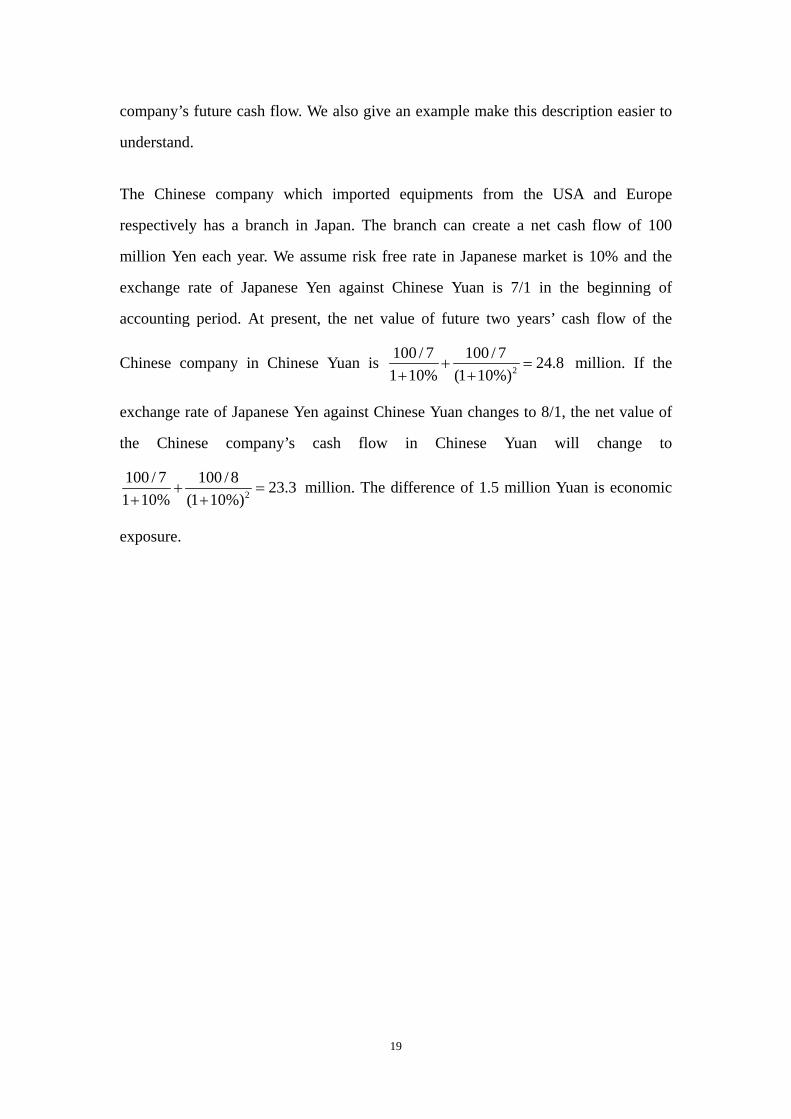
The Chinese company which imported equipments from the USA and Europe
respectively has a branch in Japan. The branch can create a net cash flow of 100
million Yen each year. We assume risk free rate in Japanese market is 10% and the
exchange rate of Japanese Yen against Chinese Yuan is 7/1 in the beginning of
accounting period. At present, the net value of future two years’ cash flow of the
Chinese company in Chinese Yuan is 2
100 / 7 100 / 7 24.81 10% (1 10%)
+ =+ +
million. If the
exchange rate of Japanese Yen against Chinese Yuan changes to 8/1, the net value of
the Chinese company’s cash flow in Chinese Yuan will change to
2
100 / 7 100 / 8 23.31 10% (1 10%)
+ =+ +
million. The difference of 1.5 million Yuan is economic
exposure.
20
3. METHODOLOGY AND DATA
In this chapter we present the way how the data are collected and the methodology
used in our research. Some sample information and different empirical models related
to this research are presented as well. Further, we describe data processing and
reliability and validity of this study.
3.1. RESEARCH APPROACH
The purpose of this thesis is to test the relationship between exchange rate and
corporate value empirically, mainly the exchange rate exposure on automakers’ value.
We investigate the corporate value changes of three different automakers which are
affected by foreign exchange rate changes. Four multinational automakers in the USA,
Japan and Europe are chosen in this research to perform a quantitative study. Data are
collected during 2000-2006. The main reference of this paper is based on previous
studies performed by Oxelheim and Wihlborg (1995) concerning microeconomic
shocks on General Motor, and Bartram (2007) concerning foreign exchange rate risk
on corporate cash flow and stock price. The model employed in this study is in some
extent based on the previous study by Christiansen (2003).
3.2. Data Collection
3.2.1. Sources of information
In this paper, the financial data is obtained from one source, “DataStream”. The
reason of collecting data from unified data source is to ensure reliability of the data.
Collecting financial data from different sources is not good for the accuracy of the
data, because different database may use different methods to calculate financial

21
figures. All financial information including financial statements of the companies,
stock prices of companies, performance of stock markets and foreign exchange rates
in this paper are extracted from this source of information.
The data collected from “DataStream” are in the raw-data form, while, for the
statistical reason the data used in regression analysis are usually returns of raw-data.
In this paper, all data used in the model are converted to return from raw-data.
Meanwhile, “ELIN” and “LIBRIS” are used to search relevant articles and previous
literatures. The website of Wikipedia is used to search explanation of definitions and
general information of companies and industry.
3.2.2. Sample
Four largest automakers in the world are selected in this paper. They are General
Motor, Toyota, Volkswagen and Ford from the USA, Japan and Germany11. In 2008,
the output of these four companies accounted for 42% of world vehicle production
(See Figure 1). In addition, Japan, China, United States and Germany are the four
largest automotive producing counties in the world. In 2008, these four countries
contributed more than 50% of the vehicle production in the world (see Figure 2). The
stock price of Ford, Toyota and Volkswagen has significant change during the period
over 2000-2006. The general trend of the stock price of Ford is downward. The stock
price is 252.75 US dollar in the beginning of 2001 while 51.39 US dollar in the end of
2006. The curve of stock price of Toyota is a “U” shape. At the two ends of the period,
Toyota’s stock price kept around 450 Japanese Yen. The lowest price is close to 180
Japanese showed in May, 2003. The change of VW’s stock price is the most erratic
one. Its price’s fluctuation is very severe in the period and the highest value is showed
in the end of the period. (See Figure 3)
11 In this paper, we treat Europe as a united market but not separated countries.

22
Top motor vehicle manufacturing companies byvolume 2008
Toyota
GM
VW
Ford
Honda
Nissan
PSA
The others
Figure 1: Top motor vehicle manufacturing companies by volume 2008
(Data come from Production Statistics", OICA. 2009)
countries of motor vehicle production
Japan
China
USA
Germany
South Korea
Brazil
Others
Figure 2 Countries of motor vehicle production
(Data come from World motor vehicle production by manufacturer: World ranking of
manufacturers 2008", OICA. 2009.)
Stock price of the Companies
0.00
100.00200.00
300.00400.00
500.00600.00
700.00800.00
900.00
Jan-00
Jan-01
Jan-02
Jan-03
Jan-04
Jan-05
Jan-06
Ford
Toyota
VW
GM
Figure 3: Stock price of companies
(The currency used to show shock price is local currency where the company based
in.)
23
We chose representative companies in each “big four” countries except China in order
to investigate if there is a relationship of foreign exchange rate exposures among the
three countries. Although China is the second largest country of automotive
manufacturing, we do not select automakers in China because that the largest
automakers based in China are joint ventures and related to the four companies we
selected. Meanwhile, the purely Chinese-fund companies lack the power of
international influence. Chinese based automakers are not typical samples we are
studying. However, we do not ignore China’s influence as the second largest market
of vehicles. In this paper, we take into account the factor of production, marketing and
competition for the studying exchange rates choosing. China is an important market
for all four companies we selected, so the impact of exchange rate changes of Chinese
Yuan will be considered.
3.2.3. Data description
We collect weekly stock return of the four selected companies to investigate the
impact of exchange rate changes on corporate value. The data of exchange rates are
collected from Datastream in three groups. To analyze the relationship between
exchange rates changes and value of the companies of General Motor and Ford, we
collect weekly exchange rate returns of US dollar against to Chinese Yuan, Japanese
Yen and Euro respectively. The respective three countries which the selected
currencies belong to have significant meaning for the two US automakers. China is
the biggest market for both of the two US automakers, Japan and Euro are the
economy which their main competitors are based on. Similar to the US case, we
collected weekly exchange rate returns of Japanese Yen against to US dollar, Chinese
Yuan and Euro, as well as Euro against to US dollar, Chinese Yuan and Japanese Yen
respectively, in order to investigate the relationship between exchange rate changes
and the corporate value of Toyota and Volkswagen. The same as General Motor and
Ford, China is the biggest market of Toyota and Volkswagen and the four companies
are competitors for each other. In addition, in order to investigate the relationship
24
between stock prices of individual companies and market performance, we collected
the weekly return of stock market index of three countries.
3.2.4. Excluded Observations
Our data is collected in the period over 2000-2006, which is between two financial
crises. The one before our data’s period is Asian financial crisis, which started in July
1997 and began to recover in 1999. The other after our data’s period is the financial
crisis we are suffering from now. This financial crisis is widely considered that started
in July 2007 and still on at present. During financial crisis, the return of corporate
stock prices and the changes of exchange rates are not normal and representative. A
model with data collected in the period of financial crisis would not represent
appropriate relationship between corporate value and exchange rate. In this paper, we
avoid the data in the periods of the two financial crises on purpose.
3.3. Methodology
We set up a model which combined three previously presented models in researches
of exchange rate exposure. The three models are used in previous studies of exchange
rate exposure from different aspects. We extract the usefulness of them to compose
our model. And, we rise four hypotheses to been argument.
3.3.1. Related Models
The classical method of exposure measurement generally employs regression analysis
of relationship between the changes of foreign exchange rate and corporate value. The
most applied one is the following two factors model:
jt j j mt j st jtR R Rα β δ ε= + + +
Where jtR refers to stock return of company j in the period of t . mtR refers to
25
index return of the whole capital market m in the period of t . And stR refers to
exchange rate return of currency s in the period of t . A lot of literatures use this
model to measure the exposure of exchange rate on corporate value. Generally,
samples used in this model are large. Economists usually choose a large number of
companies in a market (for example the world’s top 500 companies in a country or an
area) or an industry (for example all public steel companies in the world). The
exchange rate which is studied here is not the exchange rate of currency s against to
a specific currency but the trade weighted index of currency s .
Although most empirical literatures on foreign exchange rate exposure use the model
above, the literatures of risk management of exchange rate risk usually focus on
corporate cash flow. As an alternative approach of exposure measurement, the model
below is used to investigate the relationship between changes of exchange rate and
corporate cash flow changes:
CFjt j j St jtR Rα δ ε= + +
Where CFjtR refers to corporate cash flow return of company j in the period of t .
stR refers to exchange rate return of currency s in the period of t . Generally,
economists use this model to investigate individual companies since the data of
corporate cash flow is not available publically. Collecting large group’s sample of
corporate cash flow is much more difficult than collecting the data of stock prices.
Usually, authors work closely with one or limited number of companies to write
empirical literatures of exchange rate exposure on corporate cash flow. They choose a
small number of companies as sample to investigate the relationship between
exchange rate changes and changes of cash flow. In this model, the studied exchange
rate is the exchange rate of currency s against to a specific foreign currency but not
an index used in the stock price model.
As the development of global economy, the business of multinational companies is

26
commonly involved in different countries. Just study the exchange rate of domestic
currency against to one specific foreign currency for corporate cash flow is not
enough. Competitive, supplied and produced factors of exchange rate should also be
considered in the research. Oxelheim and Wihlborg provide a model of exchange rate
exposure on corporate cash flow with some macroeconomics factors considered:
1 2 3 4( / ) ( / )DC DCt t t i t i t i tCF P DC FC V Zα α α α ε− − −= + + + +
Where DCtCF refers to the nominal cash flows during the period of t in domestic
currency. DCtP refers to the price level in domestic currency in the period of t .
( / )t iDC FC − refers to the exchange rates of domestic currency against one specific
foreign exchange rate in period t i− . t iV − refers to some other macroeconomic
variables in period t i− , such as interest rate and inflation rate. t iZ − refers to firm-
and industry- specific disturbances, such as new competitor entering or new rules
making.
3.3.2. The employed model
According to efficient-market hypothesis (EMH), it is impossible to consistently
outperform the market by using any information that the market already knows. This
means that studying the relationship between the returns of exchange rates and stock
prices only does not make sense. Consequently, we use empirical volatility and mean
spillover model to study the impact of foreign exchange rate on stock price of the
three automakers in this paper. Christiansen (2003) applied a three steps’ model to
investigate the spillover effects in European bond market. The first two steps of the
model use a single variable GARCH model to estimate the return of the US bond
market (global effect) and the aggregate European return (regional effect),
respectively. The one period lagged US and European returns are used as explanatory
variables. In the third step, a single variable extend GARCH model is used to estimate
27
the return of individual European bond market.
We use the similar model to test the influence of foreign exchange rates and stock
market indexes on stock prices of the three companies we selected. First, the
conditional return on the foreign return is assumed to evolve according to an AR(1)
model:
, 0,1 1, , 1 ,i t i i t i tS S eα α −= + +
,i tS is the return of foreign exchange rate, where i represents different exchange
rate returns, such as useuS represents the return of the exchange rate of US dollar
against to Euro. The idiosyncratic shock ,i te , is normally distributed with mean 0 and
the conditional variance follows a symmetric GARCH(1,1) specification. The
GARCH model was developed independently by Engle (1982) and Bollerslev (1986):
2 2 2, , 1 , 1i t i i i t i i teσ ω α β σ− −= + +
The model allows the conditional variance to be dependent upon previous own lag.
2, 1i i teα − is the volatility during the previous period of i . 2
, 1i i tβ σ − is the fitted variance
from the model during the previous period of i . 2tσ is know as the conditional
variance since it is a one-period ahead estimate for the variance calculated based on
any past information thought relevant. Using the GARCH model it is possible to
interpret the current fitted variance as a weighted function of a long-term average
value. The reason why we use GARCH(1,1) model is that we think one period lag is
enough to pass through the affect all cross the world (we use weekly data). Since the
development of information system, the financial information could be spread
globally in the very short time.
The return of stock price of company j , ,j tR , is described by the following extended

28
AR(1) specification:
, 0, 1, , 1 2, , 1 3, , ,j t j j j t j i t j i t j tR R S e eβ β β β− −= + + + +
The return of stock price of company j depends on its own lagged return and the
lagged return of foreign exchange rate as well as the contemporary exchange rate
residual. The mean spillover effects are introduced by the lagged exchange rate return
,i tS . The volatility spillover from the exchange rate to selected companies’ stock price
takes place via the exchange rate’s idiosyncratic shock, ,i te . The idiosyncratic shock
,j te has mean 0 and the conditional variance 2,j tσ which evolves according to the
GARCH (1, 1):
2 2 2, , 1 , 1j t j j j t j j teσ ω α β σ− −= + +
In addition, individual company’s stock price is affacted by the performance of whole
of the stock market. Meanwhile, as automotive giants, each one the three companies
must influence the local stock market in some extent. In this paper, we also study the
mutual influence between market index and corporate stock price employing the same
processes as above. First, the conditional return on the foreign return is assumed to
evolve according to an AR(1) model:
, 0,1 1, , 1 ,k t k k t k tI I eα α −= + +
,k tI is the return of market index of market k , where k represents different
exchange rate returns, such as usI represents the return of stock market index of the
USA. The idiosyncratic shock ,k te , is Also normally distributed with mean 0 and the
conditional variance follows a symmetric GARCH(1,1) specification:

29
2, 1k tσ − is the shock of the exchange rate return k . The return of stock price of
company j , ,j tR , is described by the following extended AR(1) specification:
, 0, 1, , 1 2, , 1 3, , ,j t j j j t j k t j k t j tR R I e eβ β β β− −= + + + +
The one period lagged variables in the model can play the role of avoiding
autocorrelation.
3.3.3. Tests
ARCH model is standing on the heteroscedastic variances. If the variance of errors is
constant is known as homoscedasticity. If the variance of the errors is not constant,
this would be known as heteroscedasticity. If the errors are heteroscedastic the
estimators will still give unbiased coefficient estimates, but they are no longer BLUE.
That is, they no longer have the minimum variance among the class of unbiased
estimators. The heteroscedasticity of variance for foreign exchange rates will be tested
in chapter 4.
In addition, if an important variable is omitted from the equation, the consequence of
estimated coefficients on all other variables will be biased and inconsistent unless the
excluded variable is uncorrelated with all the included variables. Even if this
condition is satisfied the estimate of the coefficient on the constant term will be biased.
Consequently, all forecasts made from the model would be biased and the standard
errors will also be biased. As a result, hypothesis tests could yield inappropriate
inferences. In this paper, we use Chow test to detect if the model includes sufficient
variables or not.
Meanwhile, if the model includes an irrelevant variable, the consequence is that the
coefficient estimators would still be consistent and unbiased, but the estimators would
2 2 2, , 1 , 1k t k k k t k k teσ ω α β σ− −= + +
30
be inefficient. This would imply that the standard errors for the coefficients are likely
to be inflated relative to the values which they would have taken if the irrelevant
variable had not been included. Variables which would otherwise have been
marginally significant may no longer are so in the presence of irrelevant variables. In
this paper, we use Wald test to find out if there are irrelevant variables or not. The
tests will be present and null hypotheses will be raised in the chapter 4 for each
automaker.
3.3.4. Hypotheses
There are four hypotheses in this paper. The first one is that the appreciation of
currency in the main foreign market of the company has a positive relation with firm’s
stock price. The appreciation of the main foreign market’s currency has two aspects to
impact on corporate cash flow. First, turn over in foreign market will increased when
it is counted by local currency where the company is based in with appreciated
foreign market’s currency. Second, compared to the appreciated currency in foreign
market, local cost of the company’s products is decreased and thus the company’s
competition will be increased.
The second hypothesis is that the appreciation of currency in the main foreign
produce area of the company has a negative relation with firm’s stock price. The
appreciation of the main foreign produce area’s currency also has two aspects to
impact on corporate cash flow. First, the cost, such as labor and property cost will be
increased as the appreciation of produce area’s currency and thus corporate net cash
flow will be decreased. Second, when the increased cost is added on price, the turn
over in foreign market will decrease because of decreased competition.
The third hypothesis is that the appreciation of currency where main supplier of the
company is based in has a negative relation with firm’s stock price. It is the same as
the above two situations. Appreciation of supplier’s currency increases input price and
thus it decreases company’s net cash flow and competition in foreign market.
31
The forth hypothesis is that the stock price of an individual company is related to the
performance of the whole market where the company is based in. Stock price is a
mirror of a company’s performance, and any individual company’s performance could
not be independent from the whole market’s situation. There must be a relation
between the trend of the whole stock market and the individual corporate stock price.
3.4. Validity and Reliability
We chose to just investigate the relationship between exchange rate and corporate
stock price in the period over 2000-2006. Usually, corporate cash flow is the direct
indicator of corporate value. If we chose corporate cash flow as dependent variable
we will face a major problem as observations are not sufficient. The information of
corporate cash flow is not available daily in public. The most frequent declaration of
cash flow by company is quarterly data. Obviously, 7 years quarterly data is not
sufficient to make an empirical study. Meanwhile, we do not study data beyond the
period. As we mentioned before, there are two financial crises beyond the two ends of
the period. During financial crisis, the return of corporate stock prices and the changes
of exchange rates are not normal and representative. A model with data collected in
the period of financial crisis would not represent appropriate relationship between
corporate value and exchange rate. In this paper, we avoid the data in the periods of
the two financial crises on purpose.
3.4.1. Validity
As globalization intensifies, a company’s performance is usually not impacted by only
one exchange rate. The factors of production, competition and marketing dominate
the companies’ performance. According to operation of these companies, the factors
come from different countries. As a result, we chose different exchange rates as
variables to test their impact on corporate value.
The model employed in this paper is applied in previous related research and well
32
commented in previous literature. It is proved that the model can study volatility
efficiently. This paper only involves data collection and data processing.
3.4.2. Reliability
To ensure reliability we apply unified process of data and use only one database to
collect data. All regressions used in this paper are run using OLS in the econometrics
software EViews. It is well used software for statistical research. According to
efficient-market hypothesis (EMH), it is impossible to consistently outperform the
market by using any information that the market already knows. This means that only
studying the relationship between the returns of exchange rates and stock prices does
not make sense. Consequently, we use empirical volatility and mean spillover model
to study the impact of foreign exchange rate on stock price of the three automakers in
this paper.

33
4. EMPIRICAL FINDINGS
In this chapter, we present obtained result of regression to readers. Starting with
description of variables and data, requirements of assumption are also presented.
Specification of Empirical results and regression tests are the main contents of this
chapter.
4.1. DESCRIPTIVE STATISTICS
The weekly returns of these four companies, General Motors, Ford, Toyota and
Volkswagen, are selected as dependent variables of the model. We use RG, RF, RT and
RV to represent them. To study the impact of different exchange rate returns on the
four companies, we select exchange rate of local currency of the country where each
company is based in against three different foreign currencies. These three foreign
currencies are from countries where the company’s market, suppliers and competitors
belong to. We use SUSEU, SUSYE and SUSYU to represent three foreign exchange rate
variables which are US dollar against to Euro, Japanese Yen and Chinese Yuan
respectively of Ford. Similarly, we use SYEEU, SYEUS, SYEYU, SEUUS, SEUYE and SEUYU
to represent foreign exchange variables which are Japanese Yen against to Euro, US
dollar and Chinese Yuan as well as Euro against to US dollar, Japanese Yen and
Chinese Yuan of Toyota and Volkswagen, respectively. Exchange rates regarding to
General Motors are the same as Ford’s. We use two-way exchange rate in this paper,
such as the exchange rate of EUR against to US dollar, SEUUS, and the exchange rate
of US dollar against to EUR, SUSEU. It is because of the exchange rate of two
currencies is different in different exchange markets. In addition, stock market index
of three countries where the three companies are based in are variables in the model.
We use IUS, IEU and IJA to represent them.
34
Variable Min Max Mean Median Std.dev SUSEU -0.04038 0.039024 0.000681 0.000965 0.013659 SUSYE -0.03488 0.041882 -0.00034 -0.00047 0.012868 SUSYU -0.00152 0.020187 0.000161 0 0.001159 SYEEU -0.05863 0.039001 0.001005 0.001429 0.014345 SYEUS -0.04404 0.038187 0.000336 0.00085 0.012398 SYEYU -0.04463 0.034581 0.000502 0.000759 0.013082 SEUUS -0.03877 0.040922 -0.00068 -0.00116 0.013755 SEUYE -0.05214 0.058693 -0.00102 -0.00168 0.014463 SEUYU -0.03867 0.040924 -0.00052 -0.00097 0.013716 IUS -0.13261 0.088102 -0.0005 0.000988 0.026556 IEU -0.15819 0.105236 0.000101 0.003376 0.026126 IJA -0.10338 0.103081 -0.00081 -0.000066 0.030310
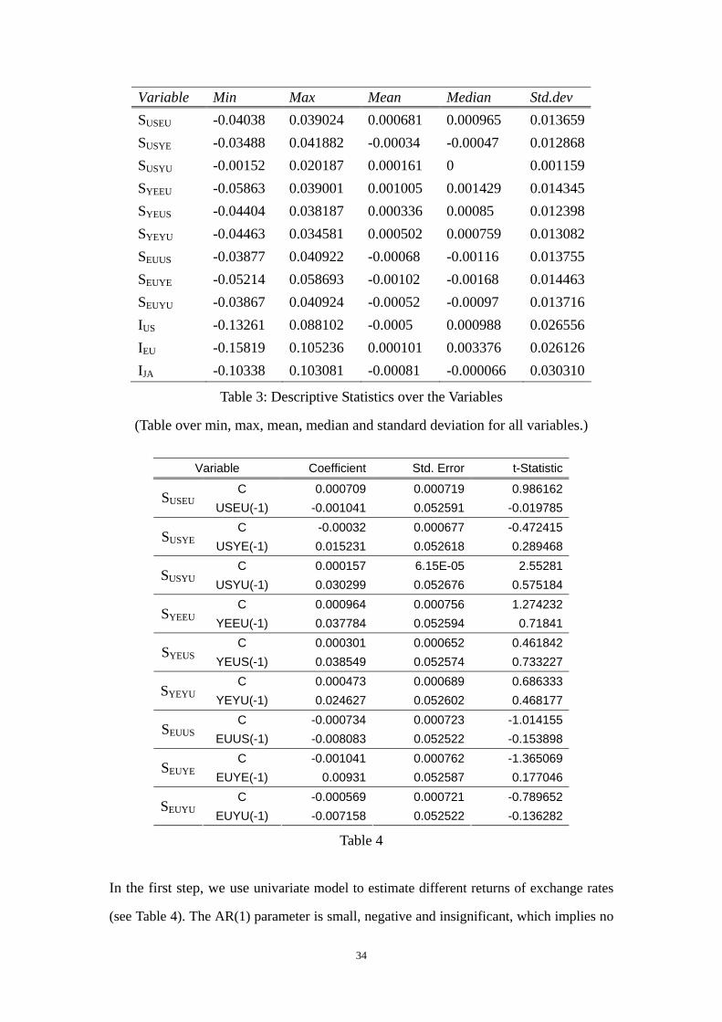
Table 3: Descriptive Statistics over the Variables
(Table over min, max, mean, median and standard deviation for all variables.)
Variable Coefficient Std. Error t-Statistic
C 0.000709 0.000719 0.986162 SUSEU USEU(-1) -0.001041 0.052591 -0.019785
C -0.00032 0.000677 -0.472415 SUSYE
USYE(-1) 0.015231 0.052618 0.289468 C 0.000157 6.15E-05 2.55281
SUSYU USYU(-1) 0.030299 0.052676 0.575184
C 0.000964 0.000756 1.274232 SYEEU
YEEU(-1) 0.037784 0.052594 0.71841 C 0.000301 0.000652 0.461842
SYEUS YEUS(-1) 0.038549 0.052574 0.733227
C 0.000473 0.000689 0.686333 SYEYU
YEYU(-1) 0.024627 0.052602 0.468177 C -0.000734 0.000723 -1.014155
SEUUS EUUS(-1) -0.008083 0.052522 -0.153898
C -0.001041 0.000762 -1.365069 SEUYE
EUYE(-1) 0.00931 0.052587 0.177046 C -0.000569 0.000721 -0.789652
SEUYU EUYU(-1) -0.007158 0.052522 -0.136282
Table 4
In the first step, we use univariate model to estimate different returns of exchange rates
(see Table 4). The AR(1) parameter is small, negative and insignificant, which implies no
35
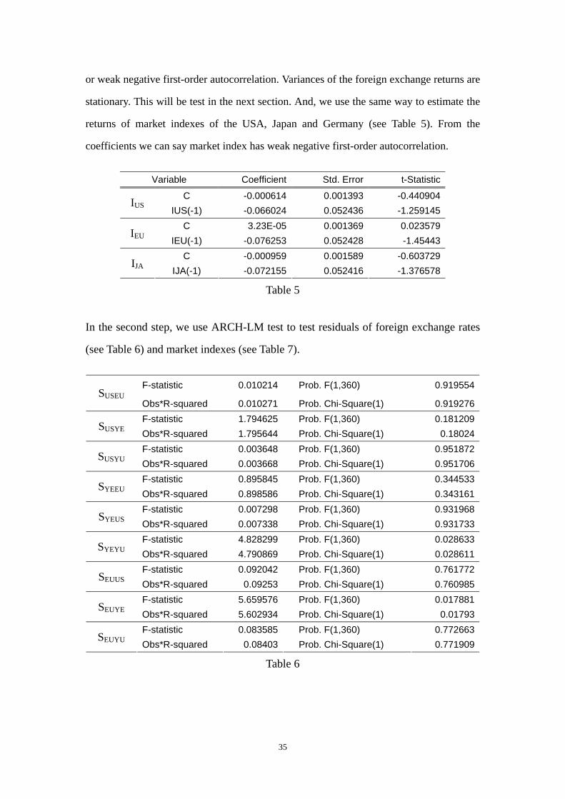
or weak negative first-order autocorrelation. Variances of the foreign exchange returns are
stationary. This will be test in the next section. And, we use the same way to estimate the
returns of market indexes of the USA, Japan and Germany (see Table 5). From the
coefficients we can say market index has weak negative first-order autocorrelation.
Variable Coefficient Std. Error t-Statistic
C -0.000614 0.001393 -0.440904 IUS IUS(-1) -0.066024 0.052436 -1.259145 C 3.23E-05 0.001369 0.023579
IEU IEU(-1) -0.076253 0.052428 -1.45443 C -0.000959 0.001589 -0.603729
IJA IJA(-1) -0.072155 0.052416 -1.376578
Table 5
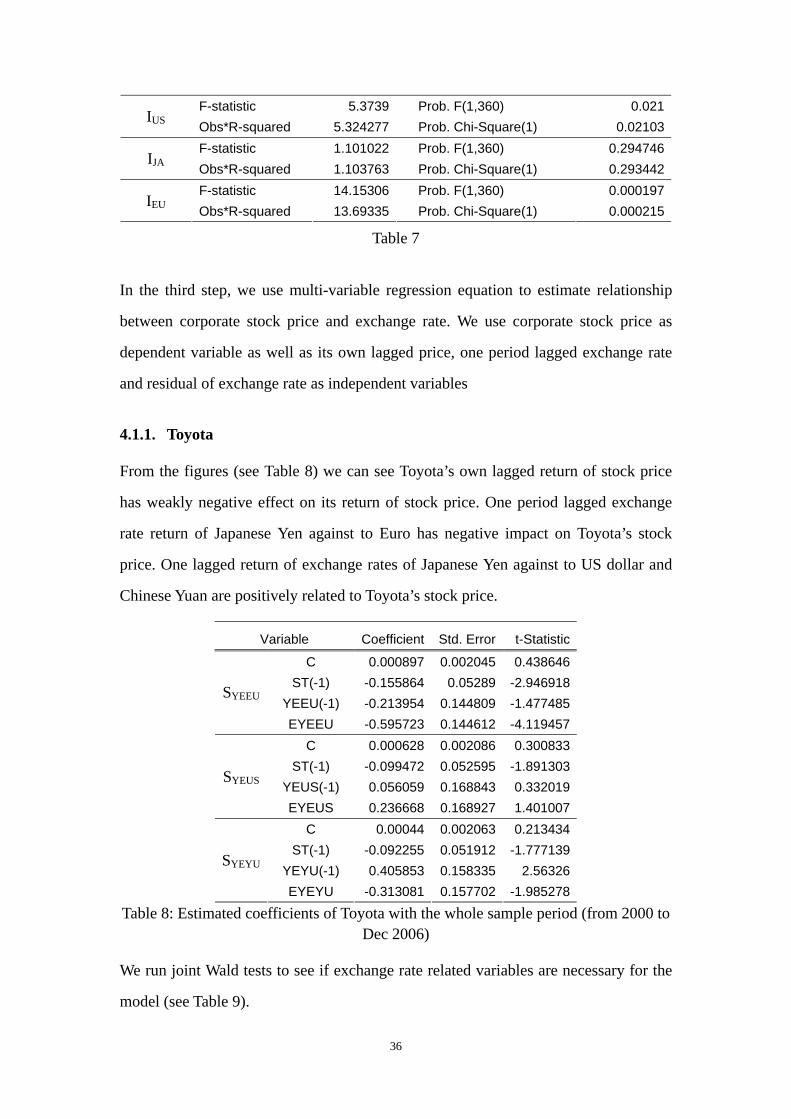
In the second step, we use ARCH-LM test to test residuals of foreign exchange rates
(see Table 6) and market indexes (see Table 7).
F-statistic 0.010214 Prob. F(1,360) 0.919554SUSEU
Obs*R-squared 0.010271 Prob. Chi-Square(1) 0.919276F-statistic 1.794625 Prob. F(1,360) 0.181209
SUSYE Obs*R-squared 1.795644 Prob. Chi-Square(1) 0.18024F-statistic 0.003648 Prob. F(1,360) 0.951872
SUSYU Obs*R-squared 0.003668 Prob. Chi-Square(1) 0.951706F-statistic 0.895845 Prob. F(1,360) 0.344533
SYEEU Obs*R-squared 0.898586 Prob. Chi-Square(1) 0.343161F-statistic 0.007298 Prob. F(1,360) 0.931968
SYEUS Obs*R-squared 0.007338 Prob. Chi-Square(1) 0.931733F-statistic 4.828299 Prob. F(1,360) 0.028633
SYEYU Obs*R-squared 4.790869 Prob. Chi-Square(1) 0.028611F-statistic 0.092042 Prob. F(1,360) 0.761772
SEUUS Obs*R-squared 0.09253 Prob. Chi-Square(1) 0.760985F-statistic 5.659576 Prob. F(1,360) 0.017881
SEUYE Obs*R-squared 5.602934 Prob. Chi-Square(1) 0.01793F-statistic 0.083585 Prob. F(1,360) 0.772663
SEUYU Obs*R-squared 0.08403 Prob. Chi-Square(1) 0.771909
Table 6
36
F-statistic 5.3739 Prob. F(1,360) 0.021IUS
Obs*R-squared 5.324277 Prob. Chi-Square(1) 0.02103F-statistic 1.101022 Prob. F(1,360) 0.294746
IJA Obs*R-squared 1.103763 Prob. Chi-Square(1) 0.293442F-statistic 14.15306 Prob. F(1,360) 0.000197
IEU Obs*R-squared 13.69335 Prob. Chi-Square(1) 0.000215
Table 7
In the third step, we use multi-variable regression equation to estimate relationship
between corporate stock price and exchange rate. We use corporate stock price as
dependent variable as well as its own lagged price, one period lagged exchange rate
and residual of exchange rate as independent variables
4.1.1. Toyota
From the figures (see Table 8) we can see Toyota’s own lagged return of stock price
has weakly negative effect on its return of stock price. One period lagged exchange
rate return of Japanese Yen against to Euro has negative impact on Toyota’s stock
price. One lagged return of exchange rates of Japanese Yen against to US dollar and
Chinese Yuan are positively related to Toyota’s stock price.
Variable Coefficient Std. Error t-Statistic
C 0.000897 0.002045 0.438646 ST(-1) -0.155864 0.05289 -2.946918
YEEU(-1) -0.213954 0.144809 -1.477485 SYEEU
EYEEU -0.595723 0.144612 -4.119457 C 0.000628 0.002086 0.300833
ST(-1) -0.099472 0.052595 -1.891303 YEUS(-1) 0.056059 0.168843 0.332019
SYEUS
EYEUS 0.236668 0.168927 1.401007 C 0.00044 0.002063 0.213434
ST(-1) -0.092255 0.051912 -1.777139 YEYU(-1) 0.405853 0.158335 2.56326
SYEYU
EYEYU -0.313081 0.157702 -1.985278
Table 8: Estimated coefficients of Toyota with the whole sample period (from 2000 to Dec 2006)
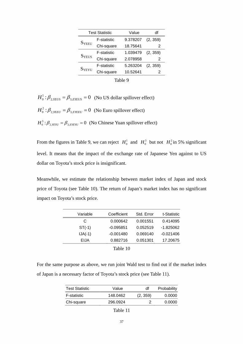
We run joint Wald tests to see if exchange rate related variables are necessary for the
model (see Table 9).
37
Test Statistic Value df
F-statistic 9.378207 (2, 359) SYEEU Chi-square 18.75641 2 F-statistic 1.039479 (2, 359)
SYEUS Chi-square 2.078958 2 F-statistic 5.263204 (2, 359)
SYEYU Chi-square 10.52641 2
Table 9
10 2, 3,: 0YEUS EYEUSH β β= = (No US dollar spillover effect)
20 2, 3,: 0YEEU EYEEUH β β= = (No Euro spillover effect)
30 2, 3,: 0YEYU EYEYUH β β= = (No Chinese Yuan spillover effect)
From the figures in Table 9, we can reject 10H and 3
0H but not 20H in 5% significant
level. It means that the impact of the exchange rate of Japanese Yen against to US
dollar on Toyota’s stock price is insignificant.
Meanwhile, we estimate the relationship between market index of Japan and stock
price of Toyota (see Table 10). The return of Japan’s market index has no significant
impact on Toyota’s stock price.
Variable Coefficient Std. Error t-Statistic
C 0.000642 0.001551 0.414095 ST(-1) -0.095851 0.052519 -1.825062 IJA(-1) -0.001480 0.069140 -0.021406 EIJA 0.882716 0.051301 17.20675
Table 10
For the same purpose as above, we run joint Wald test to find out if the market index
of Japan is a necessary factor of Toyota’s stock price (see Table 11).
Test Statistic Value df Probability
F-statistic 148.0462 (2, 359) 0.0000 Chi-square 296.0924 2 0.0000
Table 11

38
40 2, 3,: 0IJA EIJAH β β= = (No market Index spillover effect)
From the figure in Table 11, we can see the null hypothesis is strongly rejected in 5%
level. We can conclude that market index and Toyota’s stock price is related.
4.1.2. General Motors
From the figures (see Table 12), we can see that GM’s own lagged return of stock
price has no significant or weakly positive effect on its return of stock price. One
period lagged exchange rate return of US dollar against to Euro has negative impact
on GM’s stock price. One lagged return of exchange rates of US dollar against to
Japanese Yen and Chinese Yuan are positively related to GM’s stock price.
Variable Coefficient Std. Error t-Statistic
C -0.002487 0.002641 -0.941706 SG(-1) 0.001664 0.052786 0.031517
USEU(-1) -0.130276 0.19344 -0.673471 SUSEU
EUSEU -0.31972 0.192886 -1.657559 C -0.002568 0.002651 -0.968793
SG(-1) 0.003372 0.052934 0.063705 USYE(-1) 0.006174 0.205492 0.030045
SUSYE
EUSYE -0.05377 0.206006 -0.261014 C -0.002679 0.002674 -1.001982
SG(-1) 0.003179 0.052844 0.060153 USYU(-1) 0.674689 2.284371 0.29535
SUSYU
EUSYU -0.579806 2.287881 -0.253425
Table 12: Estimated coefficients of GM with the whole sample period (from 2000 to
Dec 2006)
Test Statistic Value df
F-statistic 1.603375 (2, 358) SUSEU Chi-square 3.206751 2 F-statistic 0.034507 (2, 358)
SUSYE Chi-square 0.069014 2 F-statistic 0.075643 (2, 358)
SUSYU Chi-square 0.151287 2
Table 13
39
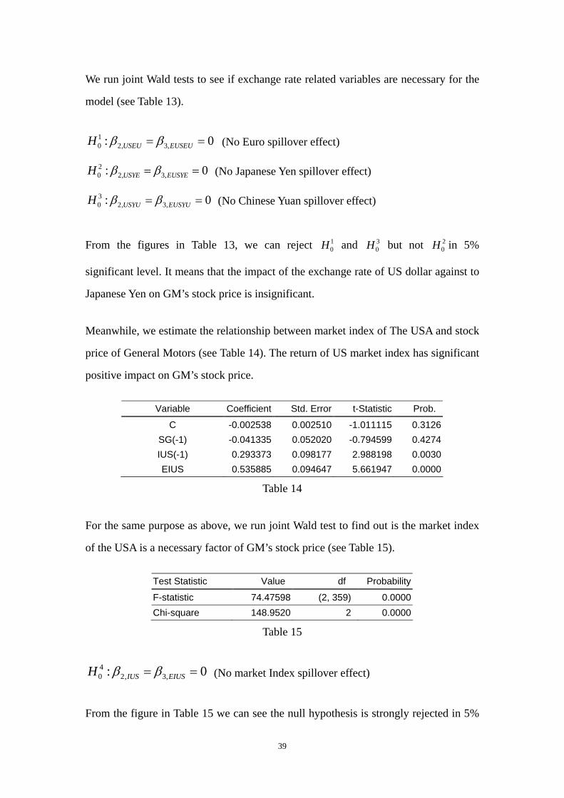
We run joint Wald tests to see if exchange rate related variables are necessary for the
model (see Table 13).
10 2, 3,: 0USEU EUSEUH β β= = (No Euro spillover effect)
20 2, 3,: 0USYE EUSYEH β β= = (No Japanese Yen spillover effect)
30 2, 3,: 0USYU EUSYUH β β= = (No Chinese Yuan spillover effect)
From the figures in Table 13, we can reject 10H and 3
0H but not 20H in 5%
significant level. It means that the impact of the exchange rate of US dollar against to
Japanese Yen on GM’s stock price is insignificant.
Meanwhile, we estimate the relationship between market index of The USA and stock
price of General Motors (see Table 14). The return of US market index has significant
positive impact on GM’s stock price.
Variable Coefficient Std. Error t-Statistic Prob.
C -0.002538 0.002510 -1.011115 0.3126 SG(-1) -0.041335 0.052020 -0.794599 0.4274 IUS(-1) 0.293373 0.098177 2.988198 0.0030 EIUS 0.535885 0.094647 5.661947 0.0000
Table 14
For the same purpose as above, we run joint Wald test to find out is the market index
of the USA is a necessary factor of GM’s stock price (see Table 15).
Test Statistic Value df Probability
F-statistic 74.47598 (2, 359) 0.0000 Chi-square 148.9520 2 0.0000
Table 15
40 2, 3,: 0IUS EIUSH β β= = (No market Index spillover effect)
From the figure in Table 15 we can see the null hypothesis is strongly rejected in 5%

40
level. We can conclude that market index and GM’s stock price is related.
4.1.3. Volkswagen
From the figures (see Table 16) we can see VW’s own lagged return of stock price has
no significant or weakly negative effect on its return of stock price. One period lagged
exchange rate return of Euro against to Japanese Yen has negative impact on VW’s
stock price. One lagged return of exchange rates of Euro against to US dollar and
Chinese Yuan are positively related to VW’s stock price.
Variable Coefficient Std. Error t-Statistic
C 0.001557 0.002354 0.661691 SV(-1) -0.041416 0.052723 -0.785543
EUUS(-1) 0.031446 0.174098 0.180625 SEUUS
EEUUS 0.64911 0.171129 3.793112 C 0.001417 0.002395 0.591841
SV(-1) -0.037937 0.052706 -0.719791 EUYE(-1) -0.113465 0.165538 -0.685432
SEUYE
EEUYE 0.232209 0.165242 1.405266 C 0.00157 0.002348 0.66847
SV(-1) -0.044138 0.05271 -0.837383 EUYU(-1) 0.057808 0.17455 0.331183
SEUYU
EEUYU 0.67639 0.171307 3.948405
Table 16: Estimated coefficients of VW with the whole sample period (from 2000 to
Dec 2006)
We run joint Wald tests to see if exchange rate related variables are necessary for the
model (see Table 17).
Test Statistic Value df Probability
F-statistic 7.21146 (2, 359) 0.0008 SEUUS Chi-square 14.42292 2 0.0007 F-statistic 1.221519 (2, 359) 0.296
SEUYE Chi-square 2.443037 2 0.2948 F-statistic 7.850832 (2, 359) 0.0005
SEUYU Chi-square 15.70166 2 0.0004
Table 17

41
10 2, 3,: 0EUUS EEUUSH β β= = (No US Dollar spillover effect)
20 2, 3,: 0euYE EEUYEH β β= = (No Japanese Yen spillover effect)
30 2, 3,: 0EUYU EEUYUH β β= = (No Chinese Yuan spillover effect)
From the figures in Table 17, we can not reject all three null hypotheses. It means that
the impact of foreign exchange rates on VW’s stock price is insignificant.
Meanwhile, we estimate the relationship between market index of The USA and stock
price of Volkswagen (see table 18). The return of EU market index has significant
positive impact on VW’s stock price.
Variable Coefficient Std. Error t-Statistic Prob.
C 0.001632 0.002015 0.809884 0.4185 SV(-1) -0.119756 0.052165 -2.295716 0.0223 IEU(-1) 0.174559 0.090632 1.926034 0.0549 EIEU 0.938512 0.077542 12.10324 0.0000
Table 18
For the same purpose as above, we run joint Wald test to find out is the market index
of Europe is a necessary factor of VW’s stock price (see Table 19).
Test Statistic Value df Probability
F-statistic 20.48637 (2, 358) 0.0000 Chi-square 40.97273 2 0.0000
Table 19
40 2, 3,: 0IEU EIEUH β β= = (No market Index spillover effect)
From the figure in Table 19 we can see the null hypothesis is strongly rejected in 5%
level. We can conclude that market index and VW’s stock price is related.
4.1.4. Ford
From the figures (see Table 20) we can see GM’s own lagged return of stock price has
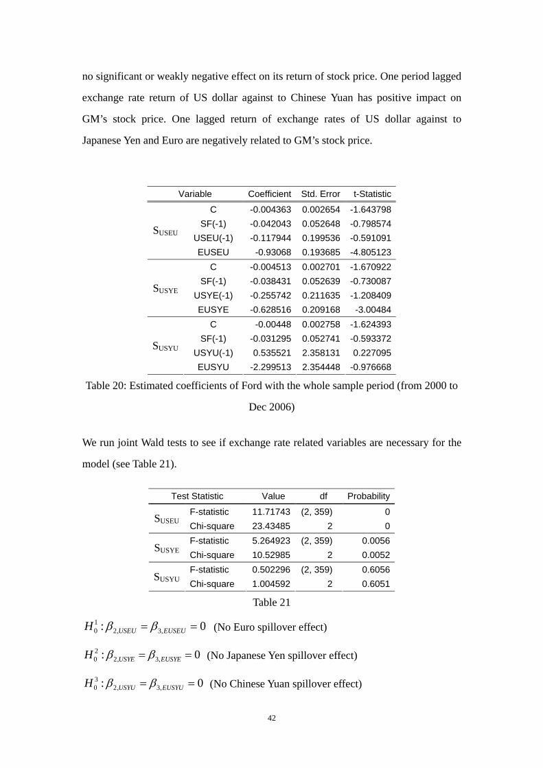
42
no significant or weakly negative effect on its return of stock price. One period lagged
exchange rate return of US dollar against to Chinese Yuan has positive impact on
GM’s stock price. One lagged return of exchange rates of US dollar against to
Japanese Yen and Euro are negatively related to GM’s stock price.
Variable Coefficient Std. Error t-Statistic
C -0.004363 0.002654 -1.643798 SF(-1) -0.042043 0.052648 -0.798574
USEU(-1) -0.117944 0.199536 -0.591091 SUSEU
EUSEU -0.93068 0.193685 -4.805123 C -0.004513 0.002701 -1.670922
SF(-1) -0.038431 0.052639 -0.730087 USYE(-1) -0.255742 0.211635 -1.208409
SUSYE
EUSYE -0.628516 0.209168 -3.00484 C -0.00448 0.002758 -1.624393
SF(-1) -0.031295 0.052741 -0.593372 USYU(-1) 0.535521 2.358131 0.227095
SUSYU
EUSYU -2.299513 2.354448 -0.976668
Table 20: Estimated coefficients of Ford with the whole sample period (from 2000 to
Dec 2006)
We run joint Wald tests to see if exchange rate related variables are necessary for the
model (see Table 21).
Test Statistic Value df Probability
F-statistic 11.71743 (2, 359) 0 SUSEU Chi-square 23.43485 2 0 F-statistic 5.264923 (2, 359) 0.0056
SUSYE Chi-square 10.52985 2 0.0052 F-statistic 0.502296 (2, 359) 0.6056
SUSYU Chi-square 1.004592 2 0.6051
Table 21
10 2, 3,: 0USEU EUSEUH β β= = (No Euro spillover effect)
20 2, 3,: 0USYE EUSYEH β β= = (No Japanese Yen spillover effect)
30 2, 3,: 0USYU EUSYUH β β= = (No Chinese Yuan spillover effect)

43
From the figures in Table 21 we can reject 10H and 2
0H but not 30H in 5%
significant level. It means that the impact of the exchange rate of US dollar against to
Chinese Yuan on Ford’s stock price is insignificant.
Meanwhile, we estimate the relationship between market index of The USA and stock
price of Ford (see Table 22). The return of US market index has weak negative impact
on Ford’s stock price.
Variable Coefficient Std. Error t-Statistic
C -0.004262 0.002368 -1.799503 SF(-1) 0.002656 0.052699 0.050392 IUS(-1) -0.031050 0.102569 -0.302725 EIUS 0.984189 0.089349 11.01510
Table 22
For the same purpose as above, we run joint Wald test to find out if the market index
of the USA is a necessary factor of Ford’s stock price (see Table 23).
Test Statistic Value df Probability
F-statistic 60.66786 (2, 359) 0.0000 Chi-square 121.3357 2 0.0000
Table 23
40 2, 3,: 0IUS EIUSH β β= = (No market Index spillover effect)
From the figure in Table 23 we can see the null hypothesis is strongly rejected in 5%
level. We can conclude that market index and Ford’s stock price is related.
4.2. RESULTS OF TESTS
4.2.1. Heteroscedasticity
We run white test for each exchange rate used in this paper to see if the residuals of exchange rate variables are heteroscedasticity or not.

44
White Test
F-statistic 0.02936 Prob. F(2,360) 0.971069 SUSEU Obs*R-squared 0.059199 Prob. Chi-Square(2) 0.970834 F-statistic 0.907453 Prob. F(2,360) 0.404472 SUSYE Obs*R-squared 1.820851 Prob. Chi-Square(2) 0.402353 F-statistic 0.007767 Prob. F(2,360) 0.992263 SUSYU Obs*R-squared 0.015664 Prob. Chi-Square(2) 0.992199 F-statistic 0.581713 Prob. F(2,360) 0.559465 SYEEU Obs*R-squared 1.169342 Prob. Chi-Square(2) 0.557289 F-statistic 0.314079 Prob. F(2,360) 0.730661 SYEUS Obs*R-squared 0.632289 Prob. Chi-Square(2) 0.728954 F-statistic 2.915409 Prob. F(2,360) 0.055462 SYEYU Obs*R-squared 5.785698 Prob. Chi-Square(2) 0.055418 F-statistic 0.055616 Prob. F(2,360) 0.94591 SEUUS Obs*R-squared 0.112124 Prob. Chi-Square(2) 0.94548 F-statistic 2.918002 Prob. F(2,360) 0.055321 SEUYE Obs*R-squared 5.790763 Prob. Chi-Square(2) 0.055278 F-statistic 0.044512 Prob. F(2,360) 0.956469 SEUYU Obs*R-squared 0.089743 Prob. Chi-Square(2) 0.95612
Table 24 From the figures (see Table 24) we can see most of the residuals of exchange rates are heteroscedastic. We dealt with it before we run the regressions.
4.2.2. Variables omitting
In previous chapter we mentioned a risk of the model that is the omission of important
variables. In this paper we use Chow test to test parameters’ stability. From the figures
in the tables below, all null hypotheses for the four companies in both two studies of
foreign exchange rate and market index can not be rejected. It means there must be
some variables ate omitted. As the reasons of the limited time and resource, we can
not find all relevant variables for this study. The authors who want to research this
object further can work with the target companies more closely.

45
Chow Breakpoint Test: 6/27/2003
F-statistic 1.164606 Prob. F(4,355) 0.32614 SYEEU Log likelihood ratio 4.732443 Prob. Chi-Square(4) 0.315868 F-statistic 1.865973 Prob. F(4,355) 0.115869
SYEUS Log likelihood ratio 7.55299 Prob. Chi-Square(4) 0.109395 F-statistic 1.754505 Prob. F(4,355) 0.137532
SYEYU Log likelihood ratio 7.106184 Prob. Chi-Square(4) 0.130382 F-statistic 0.347875 Prob. F(4,355) 0.845465
IJA Log likelihood ratio 1.420101 Prob. Chi-Square(4) 0.840694
Table 25 Toyota
Chow Breakpoint Test: 6/27/2003
F-statistic 3.625221 Prob. F(4,354) 0.006534 SUSEU Log likelihood ratio 14.53295 Prob. Chi-Square(4) 0.005775 F-statistic 1.040582 Prob. F(4,354) 0.386124
SUSYE Log likelihood ratio 4.231587 Prob. Chi-Square(4) 0.37557 F-statistic 0.973285 Prob. F(4,354) 0.422099
SUSYU Log likelihood ratio 3.959412 Prob. Chi-Square(4) 0.411527 F-statistic 1.739595 Prob. F(4,354) 0.140706
IUS Log likelihood ratio 7.046624 Prob. Chi-Square(4) 0.133445
Table 26 General Motors
Chow Breakpoint Test: 6/27/2003
F-statistic 1.159051 Prob. F(4,355) 0.328654 SEUUS Log likelihood ratio 4.710015 Prob. Chi-Square(4) 0.318366 F-statistic 1.925398 Prob. F(4,355) 0.105665
SEUYE Log likelihood ratio 7.790964 Prob. Chi-Square(4) 0.099543 F-statistic 1.197892 Prob. F(4,355) 0.311404
SEUYU Log likelihood ratio 4.866798 Prob. Chi-Square(4) 0.30124 F-statistic 2.430487 Prob. F(4,355) 0.047376
IEU Log likelihood ratio 9.807373 Prob. Chi-Square(4) 0.043801
Table 27 Volkswagen
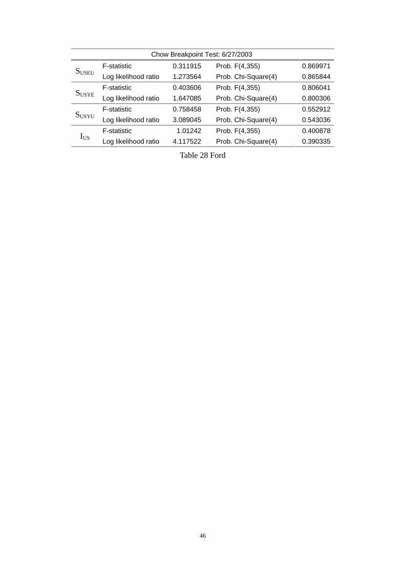
46
Chow Breakpoint Test: 6/27/2003
F-statistic 0.311915 Prob. F(4,355) 0.869971 SUSEU Log likelihood ratio 1.273564 Prob. Chi-Square(4) 0.865844 F-statistic 0.403606 Prob. F(4,355) 0.806041
SUSYE Log likelihood ratio 1.647085 Prob. Chi-Square(4) 0.800306 F-statistic 0.758458 Prob. F(4,355) 0.552912
SUSYU Log likelihood ratio 3.089045 Prob. Chi-Square(4) 0.543036 F-statistic 1.01242 Prob. F(4,355) 0.400878
IUS Log likelihood ratio 4.117522 Prob. Chi-Square(4) 0.390335
Table 28 Ford

47
5. Analysis
In this chapter, we analyze different variables’ impact on corporate stock price. The
variables are divided into two groups for analysis, as exchange rate and market index.
The hypotheses are also discussed in this chapter.
In this paper, we chose stock prices of four multinational automakers, Toyota, General
Motors, Volkswagen and Ford as independent variables, nine exchange rates (US
dollar against Euro, US dollar against Japanese Yen and US dollar against Chinese in
US exchange market; Euro against US dollar, Euro against Japanese Yen and Euro
against Chinese Yuan in European exchange market as well as Japanese Yen against
US dollar, Japanese Yen against Euro and Japanese Yen against Chinese Yuan in
Japanese exchange market) and three market indexes of the USA, Japan and Europe
as independent variables, making regression to study the relationship among them.
5.1. EFFECT OF EXCHANGE RATE ON CORPORATE STOCK
PRICE
Variables Expected Sign Obtained Sign Inferencee SYEEU + - Unexpected SYEUS + + Insignificant SYEYU + + Expected SUSEU(GM) - - Insignificant SUSYE(GM) - + Insignificant SUSYU(GM) + + Insignificant SEUUS + + Expected SEUYE + - Insignificant SEUYU + + Expected SUSEU(Ford) - - Expected SUSYE(Ford) - - Expected SUSYU(Ford) + + Insignificant
Table 29
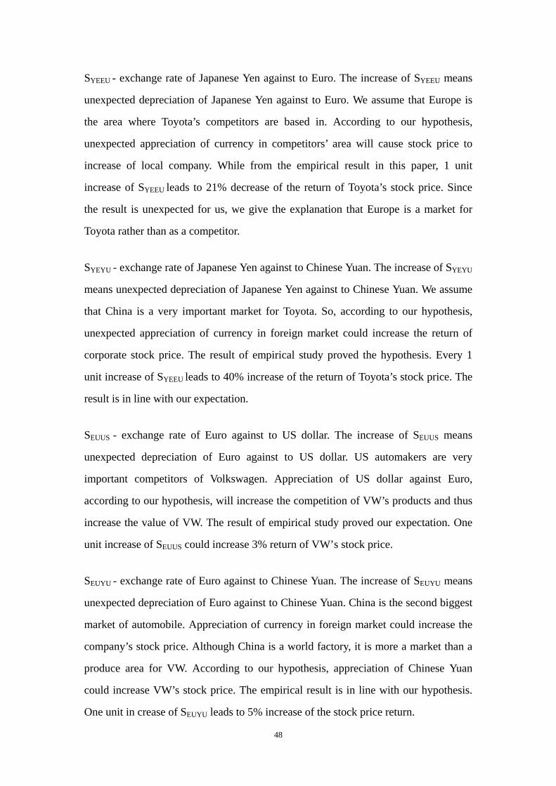
48
SYEEU - exchange rate of Japanese Yen against to Euro. The increase of SYEEU means
unexpected depreciation of Japanese Yen against to Euro. We assume that Europe is
the area where Toyota’s competitors are based in. According to our hypothesis,
unexpected appreciation of currency in competitors’ area will cause stock price to
increase of local company. While from the empirical result in this paper, 1 unit
increase of SYEEU leads to 21% decrease of the return of Toyota’s stock price. Since
the result is unexpected for us, we give the explanation that Europe is a market for
Toyota rather than as a competitor.
SYEYU - exchange rate of Japanese Yen against to Chinese Yuan. The increase of SYEYU
means unexpected depreciation of Japanese Yen against to Chinese Yuan. We assume
that China is a very important market for Toyota. So, according to our hypothesis,
unexpected appreciation of currency in foreign market could increase the return of
corporate stock price. The result of empirical study proved the hypothesis. Every 1
unit increase of SYEEU leads to 40% increase of the return of Toyota’s stock price. The
result is in line with our expectation.
SEUUS - exchange rate of Euro against to US dollar. The increase of SEUUS means
unexpected depreciation of Euro against to US dollar. US automakers are very
important competitors of Volkswagen. Appreciation of US dollar against Euro,
according to our hypothesis, will increase the competition of VW’s products and thus
increase the value of VW. The result of empirical study proved our expectation. One
unit increase of SEUUS could increase 3% return of VW’s stock price.
SEUYU - exchange rate of Euro against to Chinese Yuan. The increase of SEUYU means
unexpected depreciation of Euro against to Chinese Yuan. China is the second biggest
market of automobile. Appreciation of currency in foreign market could increase the
company’s stock price. Although China is a world factory, it is more a market than a
produce area for VW. According to our hypothesis, appreciation of Chinese Yuan
could increase VW’s stock price. The empirical result is in line with our hypothesis.
One unit in crease of SEUYU leads to 5% increase of the stock price return.
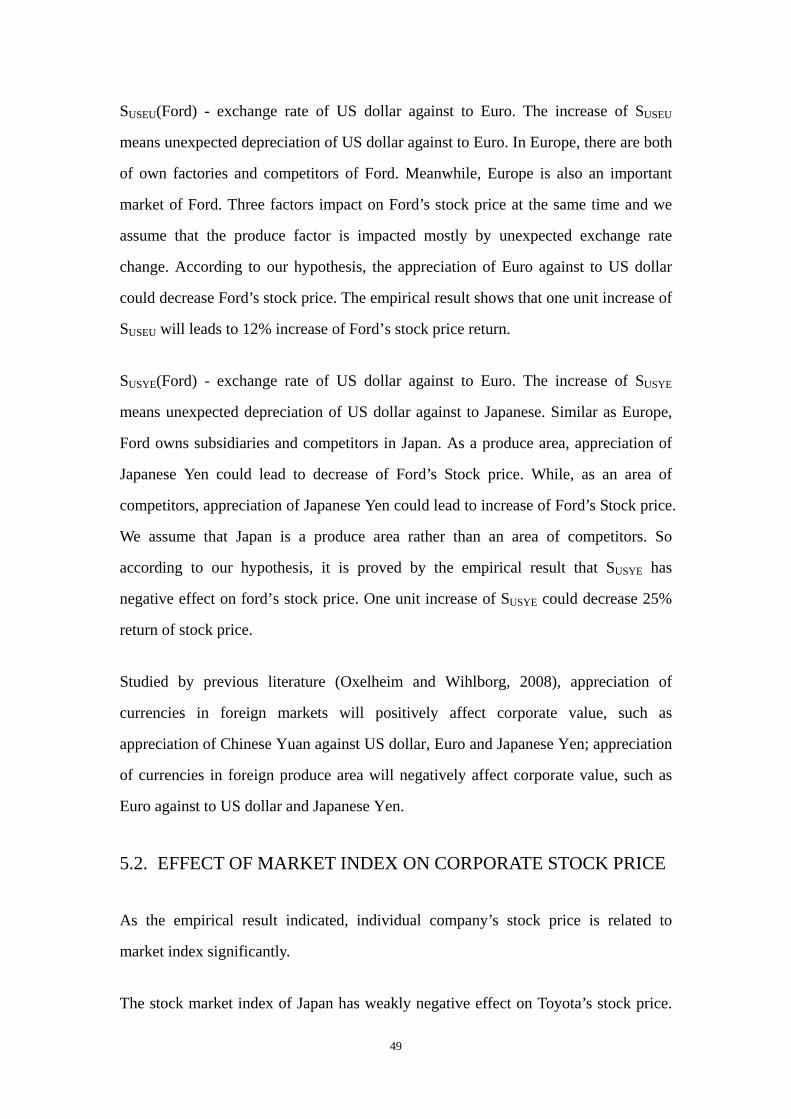
49
SUSEU(Ford) - exchange rate of US dollar against to Euro. The increase of SUSEU
means unexpected depreciation of US dollar against to Euro. In Europe, there are both
of own factories and competitors of Ford. Meanwhile, Europe is also an important
market of Ford. Three factors impact on Ford’s stock price at the same time and we
assume that the produce factor is impacted mostly by unexpected exchange rate
change. According to our hypothesis, the appreciation of Euro against to US dollar
could decrease Ford’s stock price. The empirical result shows that one unit increase of
SUSEU will leads to 12% increase of Ford’s stock price return.
SUSYE(Ford) - exchange rate of US dollar against to Euro. The increase of SUSYE
means unexpected depreciation of US dollar against to Japanese. Similar as Europe,
Ford owns subsidiaries and competitors in Japan. As a produce area, appreciation of
Japanese Yen could lead to decrease of Ford’s Stock price. While, as an area of
competitors, appreciation of Japanese Yen could lead to increase of Ford’s Stock price.
We assume that Japan is a produce area rather than an area of competitors. So
according to our hypothesis, it is proved by the empirical result that SUSYE has
negative effect on ford’s stock price. One unit increase of SUSYE could decrease 25%
return of stock price.
Studied by previous literature (Oxelheim and Wihlborg, 2008), appreciation of
currencies in foreign markets will positively affect corporate value, such as
appreciation of Chinese Yuan against US dollar, Euro and Japanese Yen; appreciation
of currencies in foreign produce area will negatively affect corporate value, such as
Euro against to US dollar and Japanese Yen.
5.2. EFFECT OF MARKET INDEX ON CORPORATE STOCK PRICE
As the empirical result indicated, individual company’s stock price is related to
market index significantly.
The stock market index of Japan has weakly negative effect on Toyota’s stock price.
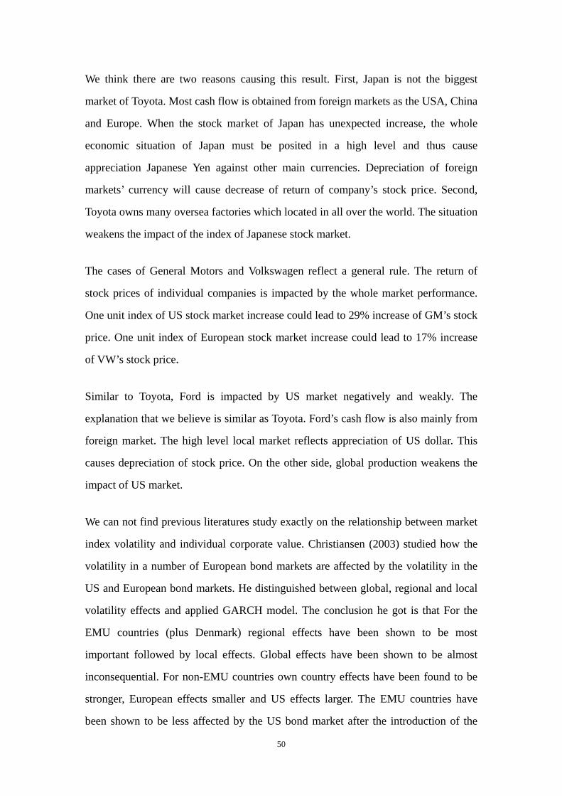
50
We think there are two reasons causing this result. First, Japan is not the biggest
market of Toyota. Most cash flow is obtained from foreign markets as the USA, China
and Europe. When the stock market of Japan has unexpected increase, the whole
economic situation of Japan must be posited in a high level and thus cause
appreciation Japanese Yen against other main currencies. Depreciation of foreign
markets’ currency will cause decrease of return of company’s stock price. Second,
Toyota owns many oversea factories which located in all over the world. The situation
weakens the impact of the index of Japanese stock market.
The cases of General Motors and Volkswagen reflect a general rule. The return of
stock prices of individual companies is impacted by the whole market performance.
One unit index of US stock market increase could lead to 29% increase of GM’s stock
price. One unit index of European stock market increase could lead to 17% increase
of VW’s stock price.
Similar to Toyota, Ford is impacted by US market negatively and weakly. The
explanation that we believe is similar as Toyota. Ford’s cash flow is also mainly from
foreign market. The high level local market reflects appreciation of US dollar. This
causes depreciation of stock price. On the other side, global production weakens the
impact of US market.
We can not find previous literatures study exactly on the relationship between market
index volatility and individual corporate value. Christiansen (2003) studied how the
volatility in a number of European bond markets are affected by the volatility in the
US and European bond markets. He distinguished between global, regional and local
volatility effects and applied GARCH model. The conclusion he got is that For the
EMU countries (plus Denmark) regional effects have been shown to be most
important followed by local effects. Global effects have been shown to be almost
inconsequential. For non-EMU countries own country effects have been found to be
stronger, European effects smaller and US effects larger. The EMU countries have
been shown to be less affected by the US bond market after the introduction of the

51
Euro.
5.3. HYPOTHESES
There are four hypotheses in this paper. The first one is that the appreciation of
currency in the main foreign market of the company has a positive relation with firm’s
stock price. This hypothesis is proved by the empirical study of the variable of SYEYU.
Since China is the second market in the world of Toyota, the appreciation of Chinese
Yuan could increase the cash flow to Toyota from China and thus increase the
performance of Toyota. This hypothesis is proved by previous study (Oxelheim and
Wihlborg, 2008).
The second hypothesis is that the appreciation of currency in the main foreign
produce area of the company has a negative relation with firm’s stock price. This
hypothesis is proved by the empirical study of the variable of SUSEU(Ford). Europe is a
very important produce area of Ford, as Ford owns many subsidiaries in Europe.
Therefore, the appreciation of Euro could decrease the cash flow to Ford from Europe
and thus decrease the performance of Ford. This hypothesis is also proved by
Oxelheim and Wihlborg (2008).
The third hypothesis is that the appreciation of currency where the main supplier of
company is based in has a negative relation with firm’s stock price. This hypothesis is
proved by the empirical study of the variable of SUSYE(Ford). Ford owns subsidiaries
in Japan. In this way, Japan is a supplier of Ford. As a consequence, the appreciation
of Japanese Yen could increase the cash flow of Ford to its suppliers in Japan and thus
decrease the performance of Ford. Oxelheim and Wihlborg (2008) concluded that
appreciation of supplier’s currency increases input price and thus it decreases
company’s net cash flow and competition in foreign market.
The forth hypothesis is that the stock price of an individual company is related to the
performance of the whole market where the company is based in. All of the four
52
companies that we selected are influenced by the stock market in their local country
and the variables of market index are proved significantly. As mentioned before, we
can not find previous literatures on the relationship between volatility of stock market
index and individual corporate value. Christiansen (2003) find out the effect between
countries is significant and Oxelheim and Wihlborg (2008) find out that the index of
consumption is significantly affect on corporate value.

53
6. Conclusion
In the last chapter of this paper, a short conclusion is presented with possible
improvements for the research in this field.
The purpose of the thesis is trying to find out the relationship between exchange rate
and corporate value. Meanwhile, it is to study whether or not there is a relationship
between individual company’s stock price and performance of the whole stock
market.
We chose four biggest automakers, Toyota, General Motors, Volkswagen and Ford in
the world as our samples to study the impact of foreign exchange rate on their stock
price. Incidentally, the relationship between market performance and individual
company’s performance is empirically estimated. We collected weekly data of nine
exchange rates and three stock market indexes during the period 2000-2006 as
independent variables to run regressions with the four companies’ stock prices.
Five variables out of nine exchange rates are proved insignificant for corporate stock
price. Appreciation of Chinese Yuan against to Japanese Yen and Euro is showed by
empirical result to have positive effect on Toyota and Volkswagen’s stock price,
whereas the appreciation of Euro against to Japanese Yen and US dollar causes Toyota
and Ford’s stock price to decrease. The empirical result also shows that Japanese
Yen’s appreciation has a negative effect on Ford’s stock price. All three variables of
stock price indexes are proved to be significantly related with corporate stock price.
However, the impact of significant variables on corporate stock price is weak.
Considering four out of nine variables are insignificant, we conclude that the impact
of exchange rate on automakers is weak.
The results of empirical study verified the hypotheses raised in the beginning of this
54
paper. Although the impact of exchange rate between Japanese Yen and Euro is
unexpected from our assumption, we get reasonable explanation for it. All four
hypotheses are supported by the empirical results in this paper: the appreciation of
currency in the main foreign market of the company has a positive relation with firm’s
stock price; the appreciation of currency in the main foreign produce area of the
company has a negative relation with firm’s stock price; the appreciation of currency
where main supplier of the company is based in has a negative relation with firm’s
stock price; the stock price of an individual company is related to the performance of
the whole market where the company is based in.
This paper could be used to study the impact of exchange rate on public companies’
performance. Further research in this area could do more in-depth study on the
analysis of the company’s operation in order to get sufficient information of the
company’s production, competition and marketing. More variables could be chosen to
study the sufficient and correct factor impacting on corporate stock price

55
Reference
Adler, M. and B. Dumas, (1984), ‘Exposure to Currency Risk: Definition and
Measurement’, Financial Management 13, 41-50.
Bartram, S. M., Dufey, G. and Frenkel, M. R. (2005), ‘A primer on the exposure of
non-financial corporations to foreign exchange rate risk’, Available online at
www.sciencedirect.com
Bartram, S. M. (2007), ‘Corporate cash flow and stock price exposures to foreign
exchange rate risk’, Journal of Corporate Finance 13, 981-994.
Bartram, S. M. and Bodnar, G. M. (2007), ‘The exchange rate exposure puzzle’,
Managerial finance 33, 642-666.
Bartram, S. M. (2006), ‘What lies beneath foreign exchange rate exposure, hedging
and cash flows’, Journal of Banking &Finance 32, 1508-1521.
Blenman, L. P., Lee, B. and Walker, M. (2006), ‘Measuring Foreign Exchange
Exposure In US Multinationals: An Empirical Investigation (1985-1997)’
Christiansen, C. (2003), ‘Volatility-Spillover Effect in European Bond Markets’,
Centre for Analytical Finance, Aarhus School of Business.
Chowdhry, B. (2009), ‘Corporate Hedging of Exchange Risk When Foreign Currency
Cash Flow is Uncertain’, Institute for Operation Research and the Management
Sciences 41, 1083-1090.
Chowdhury, A. R. (1993), ‘Does exchange rate volatility depress trade flows?
Evidence from error correction model’, Review of Economics and Statistics 75, 700
–6.
Choi, J. J. (1986), ‘A Model of Firm Valuation with Exchange Exposure’, Journal of
56
International Business Studies 2, 153-160.
De Grauwe, P. (1988), ‘Exchange rage volatility and the slowdown in growth of
international trade’, IMF Staff Papers, 35, 63–84.
Dominguez, Kathryn, M. E. and Tesar, L. L. (2001), ‘Exchange rate exposure’,
Journal of International Economics 68, 188-218.
Griffin, J.M. and Stulz, R.M. (2001), ‘International competition and exchange rate
shocks: a cross-country industry analysis of stock returns’, Review of Financial
Studies 14 (1), 215–241.
Gotur, P. (1985), ‘Effects of exchange rate volatility on trade: some further evidence’,
IMF Staff Papers, 32, 475–512.
Hooper, P. and Kohlhagen, S. (1978), ‘The effect of exchange rate uncertainty on the
prices and volume of international trade’, Journal of International Economics 8, 483
–511.
Jorion, P. (1990), ‘The exchange-rate exposure of United-States multinationals’,
Journal of Business 63, 331–345.
Kim, K-H. (2002), ‘Dollar exchange rate and stock price: evidence from multivariate
cointegration and error correction model’, Review of Financial Economics 12,
301-313.
Lin, L., Shyu, D. and Kuo, C-J. (2007), ‘The Exchange Rate Exchange of Chinese and
Taiwanese Multinational Corporations’, Journal of American Academy of Business,
Cambridge.
Mohsen, B-O. and Hegerty, S. W. (2007), ‘Exchange-rate risk and U.S.-Japan trade:
Evidence from industry level data’, J. Japanese Int. Economics 22, 518-534.
57
Mohsen, B-O. and Wang, Y. (2009), ‘Exchange Rate Sensitivity of Australia’s Trade
Flow: Evidence From Industry Data’, The Manchester School 77, 1463-6786.
Nieh, C. C., Lin, J. B. and Wang, L. S. (2009), ‘ Exchange rate uncertainty and
corporate values: evidence from Taiwan’, Applied Financial Economics.
Oxelheim, L. (1999), ‘Applying ‘MUST’ Analysis and the Role of Government in CI’,
Competitive Intelligence Review 10, 65-73.
Oxelheim, L. and Wihlborg, C.G. (1995), ‘Measuring macroeconomic exposure: the
case of Volvo cars’, European Financial Management 1 (3), 241–263.
Pan, Y. (2002), ‘Evaluation of Foreign Exchange Risk Based on Financial Data
mining: Evidence from Iron and Steel Industry in China’, Wuhan university.