Foreign Direct Investment and Export Diversification in ... Theses 2009/Shasheen...FDI and Export...
84
The University of New South Wales Australian School of Business | School of Economics ____________________ Foreign Direct Investment and Export Diversification in Low Income Nations ____________________ Shasheen Jayaweera* Honours Thesis October 2009 Bachelor of Commerce (Accounting & Finance) Bachelor of Economics (Honours) Supervised by: Dr. Nigel Stapledon * the author can be contacted at shasheenj(at)gmail.com or +61 425 250 631
Transcript of Foreign Direct Investment and Export Diversification in ... Theses 2009/Shasheen...FDI and Export...

The University of New South Wales Australian School of Business | School of Economics
____________________
Foreign Direct Investment and
Export Diversification in Low Income Nations
____________________
Shasheen Jayaweera*
Honours Thesis October 2009
Bachelor of Commerce (Accounting & Finance) Bachelor of Economics (Honours)
Supervised by: Dr. Nigel Stapledon
* the author can be contacted at shasheenj(at)gmail.com or +61 425 250 631

FDI and Export Diversification in Low Income Nations 2 of 84
Declaration of Originality
I, Shasheen Dileepa Jayaweera, declare that this thesis is my own work, and that any
contributions or materials by other authors have been appropriately acknowledged. This
thesis has not been submitted to any other university or institution as a requirement for a
degree or other award.
Shasheen Dileepa Jayaweera
26th October 2009

FDI and Export Diversification in Low Income Nations 3 of 84
Acknowledgements
I would like to acknowledge the kind and valuable support of a number of people over
the course of this year who have helped me make this project a reality.
Firstly I would like to thank my supervisor Dr. Nigel Stapledon for his guidance
throughout the year and for always challenging me to think differently and push new
boundaries with this project. I am also very grateful to Dr. Arghya Gosh for helping me
understand trade models and to Professor Denzil Fiebig for his helpful econometric
advice. I would also like to thank Professor Andy Tremayne and Dr. Valentyn Panchenco
for their econometric guidance and Dr. Gautam Bose for fuelling my interests in
development economics. I am also very grateful to the Australian School of Business for
their generous financial support during my honours year and to the UNSW Co-op
program for a fulfilling undergraduate learning experience.
This project also could not have been completed without the generous support of the
World Bank who supported the masses of trade data I required. For their support I would
like to thank Nigel Roberts, Dr. Denisse Pierola, Tomas Ernst, and Harinder Jassal.
I would also like to thank my honours colleagues for their support and for being a great
group to work with. Furthermore, I owe a special note of thanks to Rahul Nath for his
mathematical guidance and for helping me understand economic modelling.
Finally, I would like to thank my family for their priceless support and my friends who
have inspired and motivated me through all my adventures.

FDI and Export Diversification in Low Income Nations 4 of 84
Abstract
This paper seeks to understand whether increased foreign direct investment (FDI) can
help low income nations to diversify their export bases. Numerous governments in low
income nations have sought to attract FDI with an aim of diversifying their export bases
while many large multilateral development organisations have also advocated such
policies. Using Melitz’s (2003) trade model, I identify a number of potential drivers of
export diversification including firm productivity, the cost of trade, the fixed costs of
export market entry and consumer preferences and incomes. In the literature on FDI, a
number of theoretical and empirical studies link FDI to these drivers of export
diversification. These linkages are primarily based on FDI leading to improved
productivity in the host nation, together with a number of spillover benefits which help
local firms to become export competitive leading to an increase in export diversification.
I construct a rich panel dataset of 29 low income nations from 1990 to 2006 and employ
an instrumented variables estimation technique using differenced data to test the link
between FDI and export diversification. The results suggest a positive association
between increases in FDI and increases in export diversification and provide support for
the spillover argument. The results also find that this effect is reversed for nations which
export a high proportion of oil and mineral resources. Furthermore, the value in signing
free trade agreements with import partner nations is reinforced as these are found to be
associated with improved export diversification.

FDI and Export Diversification in Low Income Nations 5 of 84
Contents
1 INTRODUCTION ....................................................................................................................7
2 BACKGROUND: THE BENEFITS OF EXPORT DIVERSIFICATION................................ 12
2.1 DEFINING EXPORT DIVERSIFICATION .......................................................................... 12 2.2 THE BENEFITS OF EXPORT DIVERSIFICATION.............................................................. 13
2.2.1 Export Diversification and Overall Export Growth ..................................... 14 3 LITERATURE REVIEW....................................................................................................... 17
3.1 EXPORT DIVERSIFICATION: THEORETICAL PERSPECTIVES ........................................... 17 3.2 FDI AND EXPORT DIVERSIFICATION............................................................................ 19 3.3 EXPORT DIVERSIFICATION: EMPIRICAL PERSPECTIVES................................................ 24
4 MODELLING EXPORT DIVERSIFICATION....................................................................... 27
4.1 THE MELITZ MODEL .................................................................................................. 27 4.2 INTERPRETING EXPORT DIVERSIFICATION IN THE MODEL............................................. 31 4.3 INTERPRETING THE THEORETICAL EFFECT OF FDI ON EXPORT DIVERSIFICATION ......... 34
5 DATA ................................................................................................................................... 36
5.1 THE PRIMARY DATASET............................................................................................. 37 5.2 MEASURING EXPORT DIVERSIFICATION ...................................................................... 39 5.3 FDI DATA ................................................................................................................. 41 5.4 SELECTION OF SAMPLE OF EXPORTING NATIONS........................................................ 42 5.5 OTHER EXPLANATORY VARIABLES ............................................................................. 43 5.6 STYLIZED FEATURES OF THE DATA............................................................................. 44
6 ECONOMETRIC ESTIMATION........................................................................................... 54
6.1 DATA CONSIDERATIONS ............................................................................................ 54 6.2 ESTIMATION IN LEVELS .............................................................................................. 56 6.3 ESTIMATION IN DIFFERENCES .................................................................................... 59
7 RESULTS ............................................................................................................................ 61
7.1 LEVELS MODEL ......................................................................................................... 63 7.2 DIFFERENCED MODEL ............................................................................................... 68 7.3 EXTENSIONS ............................................................................................................. 74
8 CONCLUSION AND POLICY IMPLICATIONS .................................................................. 76
9 REFERENCES .................................................................................................................... 78
10 APPENDIX........................................................................................................................... 83

FDI and Export Diversification in Low Income Nations 6 of 84
List of Tables
Table 5.1 Datasets Created.................................................................................................... 36 Table 5.2 Import Partner Nations: Imports (US$bn 2006) ...................................................... 38 Table 5.3 Exporting Nations: Exports (US$m 2006)............................................................... 39 Table 5.4 Exporting Nations: GDP and GNI (2006)................................................................ 42 Table 6.1 P-Values from Pesaran’s CADF test ...................................................................... 55 Table 7.1 Summary Statistics – Aggregate Dataset ............................................................... 61 Table 7.2 Summary Statistics – Differenced Aggregate Dataset ........................................... 62 Table 7.3 Summary Statistics – Bilateral Dataset................................................................... 62 Table 7.4 Levels Model Results – Aggregate Dataset ........................................................... 66 Table 7.5 Levels Model Result – Bilateral Dataset................................................................. 67 Table 7.6 Differenced Model Results – Aggregate Dataset ................................................... 71 Table 10.1 Levels Model Result – Extended Bilateral Dataset................................................. 83 Table 10.2 Differenced Model, Alternate Results – Aggregate Dataset................................... 84
List of Figures
Figure 2.1 Components of Export Growth ............................................................................... 15 Figure 4.1 The Domestic Production Decisions of Firms......................................................... 29 Figure 4.2 Exporting and Non-Exporting Firms in the Domestic and Export Markets ............. 31 Figure 4.3 Export Diversification through a Change in Productivity......................................... 33 Figure 4.4 Export Diversification through a Change in Fixed Costs ........................................ 34 Figure 5.1 Map of the Sample Countries ................................................................................. 38 Figure 5.2 Counts of Bilateral Export Lines ............................................................................. 44 Figure 5.3 Counts of Bilateral Exports (Normalised with 1990=1)........................................... 45 Figure 5.4 Counts of Export Partner Nations ........................................................................... 46 Figure 5.5 Counts of Product Categories Exported ................................................................. 46 Figure 5.6 Export Counts and GDP (2006).............................................................................. 47 Figure 5.7 Export Counts and Export Partner GDP (2006) ..................................................... 48 Figure 5.8 Export Counts and Bilateral Distance..................................................................... 48 Figure 5.9 FDI Stock (US$m)................................................................................................... 49 Figure 5.10 Average FDI/GDP (%) and Total FDI Inflows (US$m) 1990-2006 ......................... 50 Figure 5.11 Comparing Log FDI Stock and Log Export Counts ................................................ 51 Figure 5.12 Comparing Log FDI Stock and Log Export Counts by Country.............................. 51 Figure 5.13 Comparing the Growth of FDI Stock and the Growth of Export Channels ............. 52 Figure 5.14 Country Level Time Trends: (Log FDI Stock and Log Export Counts) ................... 53 Figure 7.1 Scatter Plots of the Fitted Values from the IV Regression ..................................... 72 Figure 7.2 Scatter Plots of the IV Regression Residuals......................................................... 73
FDI and Export Diversification in Low Income Nations 7 of 84
1 Introduction
The dramatic rise of exports from low income nations has been one of the most
prominent economic trends witnessed over the past three decades. While economic
growth led by exports saw millions lifted out of poverty in the newly industrialising
nations of East-Asia, many other small, low income nations have only recently begun to
target exports as a channel for development. Some have already begun to reap the
benefits of such policies. For example, Cambodia’s new export orientated garments
industry has created tens of thousands of new jobs, many for women from rural areas. A
less discussed, but potentially more significant aspect of this export growth has been the
changing composition and diversity of the export bases of low income nations as these
changes may be more important in influencing overall economic development. While
almost all low income economies have managed to diversify their export bases, vast
differences exist between their diversification experiences.
Almost every major international institution including the World Bank, the United
Nations and the OECD, have advocated the benefits of export diversification.
Furthermore, a number of studies including Lederman and Maloney (2007), Herzer and
Nowak-Lehmann (2006) and Ghosh and Ostry (1994), have also noted a number of
benefits accruing to economies with diversified export bases including lower terms of
trade volatility and increased macroeconomic stability. In addition to these benefits,
Hesse (2008) also suggests that developing nations which diversified their export bases
also experienced higher income growth rates. Export diversification has also been found
to contribute to export growth especially in low income nations. Brenton and Newfarmer
(2007) found that export diversification accounted for 57% of the total export growth in
some African nations.
It should be of no surprise then that the governments of many developing countries are
striving to diversify their nation’s export bases. What is interesting, however, is that

FDI and Export Diversification in Low Income Nations 8 of 84
many are also concurrently seeking to attract increased longer term capital flows or
foreign direct investment (FDI), not just for its perceived direct economic benefits, but
also due to a belief that FDI may contribute towards the export diversification process.
Many low income nations have experienced large increases in FDI inflows and have
engaged in competition with their neighbours to attract FDI, often by offering significant
incentives. The export development and export diversification strategies of Pakistan,
Kenya, Botswana and Cambodia all make direct reference to an important role for FDI to
help boost competitiveness and develop new export industries while the World Bank has
proposed a similar strategy for Bolivia to help reduce their reliance on primary
commodity products (World Bank, 2009). The motives of Kenya’s export diversification
policy also centre on a move away from primary commodity products and increasing the
quality of manufactured exports (International Trade Centre, 2001). Many other countries
including Costa Rica, Mauritius and Chile have also had similar policies in the past. Both
Costa Rica and Mauritius partly credit their diversification into the electronics industry as
being driven by FDI flows.
While large bodies of literature have examined the drivers of export diversification, the
importance of export diversification, and the benefits of FDI, only a few have explored
the links between FDI and export diversification. Specific case studies of instances where
FDI helped develop new export industries have been documented in many countries
including India (Banga, 2003), and Bangladesh (Rhee, 1990). Yet to my knowledge, no
studies have sought to develop a theoretical connection between FDI and export
diversification. Furthermore, no papers have explored this connection empirically despite
the fact that many governments seek to attract FDI to assist with export diversification.
In an attempt to shed some light on this vital area of policy in low income nations, this
paper seeks to answer the following questions:
1. What are the theoretical mechanisms through which FDI may influence the
diversity of the export baskets of low income nations?
2. Does the empirical evidence support the argument that FDI helps recipient nations
to diversify their export baskets?

FDI and Export Diversification in Low Income Nations 9 of 84
3. Given the findings from the above two questions, what policy implications can be
drawn for low income nations to help them on their path of economic
development?
I adopt a commonly used definition of export diversification, being a growth in the
‘extensive margin’ of exports, similar to definitions in numerous studies including
Brenton and Newfarmer (2007). The extensive margin has both a geographical and
product variety dimension and export diversification occurs when either:
1. A non-exporting industry producing a specific product variety begins to export,
thus increasing the number of product varieties the nation exports; or,
2. An industry which is already exporting a specific product variety begins to export
that variety to a new destination market which it did not export to previously.
While the literature has proposed a variety of methods to measure export diversification, I
adopt a simple and widely used count indicator of the number of product categories
exported between pairs of countries. Changes in both the geographical and product
dimensions of export diversification will register as a change in the proposed ‘count of
bilateral export channels’ indicator. An increase in this count variable would constitute a
diversification of exports.
Two key areas of research are then considered to form a theoretical basis for answering
the key questions posed in this thesis. The first involves understanding the drivers of
export diversification while the second involves understanding the effects of FDI and any
interactions it may have on the drivers of export diversification.
In developing a theoretical frameset for understanding the drivers of export
diversification, I draw heavily on Melitz’s (2003) trade model which has been used
widely in recent trade literature due its rich predictions. Melitz’s model introduces the
notion of heterogenous firms (in terms of productivity) to monopolistically competitive
industries with increasing returns to scale and differentiated products. Firms must incur
fixed costs to begin producing for the domestic market and, due to differences in

FDI and Export Diversification in Low Income Nations 10 of 84
productivity and thus marginal costs, only the most productive firms find it profitable to
produce for the domestic industry. A further fixed cost must be incurred if a firm is to
establish an export market for its products and a per-unit cost of trade must also be
forfeited to reach each export market. As such, only some of the most productive firms
find it profitable to export. In some industries, no firms may find it profitable to export,
while in others, firms may only export to a few destinations.
The model predicts that changes to foreign consumer preferences, firm productivity, or
trade costs may all influence whether a firm may find it profitable to export. As a result,
these factors also influence the diversification pattern of a nation’s export base. If a firm
in a previously non-exporting sector finds it profitable to begin exporting and does so,
then their nation would effectively begin exporting a new product and thus diversify.
Existing export firms may also be induced to now begin exporting their products to a new
destination market, also constituting export diversification.
In the literature on FDI, a number of studies suggest linkages between FDI and the key
drivers of export diversification described above. Gorge and Greenway (2004), Markusen
and Venables (1999), and Kugler (2005) find both theoretic and empirical evidence that
FDI may contribute towards firm productivity. Backward linkages, learning effects and
increased domestic competition were commonly cited as channels through which FDI
may have productivity enhancing spillovers to other firms in the host nation. Other
studies including Crespo and Fontoura (2007), Aitken, Hanson, Harrison (1997) and
Kokko, Tansini and Zejan (1997), argue that there are additional spillover effects (such as
those pertaining to an information nature on foreign markets) which may even reduce the
fixed costs of ‘discovering’ and establishing export markets, another key driver of export
diversification. As a result, I find a theoretical foundation upon which export
diversification may be seen as being influenced by FDI and next move to test this
empirically.
I construct a rich panel dataset using highly disaggregated, 6-digit level, bilateral mirror
export data obtained from the UN Commodity Trade Statistics Database (COMTRADE)
for 29 of the poorest developing nations between 1990 and 2006. I calculate a count

FDI and Export Diversification in Low Income Nations 11 of 84
indicator of the number of active 6-digit level product categories exported between each
of the exporter nations and each of 21 significant importing partner nations, as a measure
of the level of export diversification. Overall, the data confirms a general pattern of
increasing diversification and exports across the sample of countries, however with
significantly varying magnitudes of change. The reasons for these differences in
diversification experiences and the question of whether FDI has contributed to the pattern
of increased diversification are the prime motives of this study. Data on other explanatory
variables including FDI, GDP, exchange rates, and trade agreements were also collected
and used to enhance the estimation of the partial effects of changes in the FDI.
I initially employ simple fixed effects and random effects models to estimate the effects
of FDI on export diversification in levels. While the signs of the estimators from these
regressions were as predicted by my theoretical discussion, evidence of spurious results
were found and thus little emphasis was placed on these models. I then adopt another
commonly used model estimating the effects in differences using an instrumental variable
dynamic panel approach to control for non-stationarity and omitted variables. Post
estimation diagnostics found the model to be robust and no evidence of non-stationarity
was found in the errors. Using this model, I find that FDI has a positive effect on the
number of export counts. Furthermore, positive coefficients estimated on the lagged FDI
variables possibly indicate the effects of spillovers which help other sectors to also begin
exporting a few years after the FDI investment was made, consistent with the effects
described in the theoretical literature.
In section 2, I present a background discussion on the benefits of export diversification
and its importance in contributing towards export and economic growth. Section 3 then
reviews the theoretical models in the literature which have been used to understand the
patterns of export diversification and the potential influences of FDI. I then present an
overview of the Melitz model in section 4 which I use to describe the drivers of export
diversification. The data and its stylised features are introduced in section 5 and the
empirical estimation techniques are discussed in section 6. The results of the empirical
estimation are presented in section 7 and the conclusions and policy implications drawn
from these are detailed in section 8.

FDI and Export Diversification in Low Income Nations 12 of 84
2 Background: The Benefits of Export Diversification
The benefits of export diversification, while not the focus, are the prime motivation for
this study which aims to understand if FDI plays a role in driving export diversification.
After defining export diversification, I provide a brief overview of its benefits before then
introducing the literature on the forces driving it.
2.1 Defining Export Diversification Studies to date have employed a number of methods to describe and then measure export
diversification. While most of the differences between these studies have centred on the
measurement of diversification1, many of these differences have also been subtle and they
are generally in agreement on the definition of diversification itself. Recent studies have
generally considered export diversification from a bilateral angle as an increase in the
number of product varieties exported between country pairs. Besedes and Prusa (2008),
Carrère, Strauss-Kahn and Cadot (2007), and Brenton and Newfarmer (2007) all describe
export diversification as the export of new product varieties to existing or new destination
markets, or the export of currently exported product varieties to new markets. In effect,
there is a geographic and product level aspect of diversification. Such patterns are also
collectively referred to as the “extensive margin” of trade in a number of studies.
As an illustrative example, assume Benin exported only one product, say coffee beans,
and exported that to only one country, say France. In the next year, suppose they then
exported another product variety such as bananas, to France. As this constitutes the
export of a new, previously non-exported variety, then this would be an example of
1 The measurement of diversification will be discussed in section 5.2

FDI and Export Diversification in Low Income Nations 13 of 84
diversification. Furthermore, if Benin were to now begin exporting coffee to another
market, say Germany, then this too would constitute as growth in its ‘extensive margin’.
2.2 The Benefits of Export Diversification Many multilateral organisations have called for greater export diversification in
developing nations. In the preface to a recent OECD working paper2, the director of the
OECD Development Centre Louka Katseli described that many low income nations
pursue export diversification strategies to ensure export price stability and to foster
income growth and that it was in the OECD’s interests to help them achieve this.
Furthermore, the final report from the World Bank led Commission on Growth and
Development (2008) also called on governments to promote policy leading to export
diversification.
Hesse (2008) suggests that export diversification could assist developing countries in
overcoming export instability, terms of trade shocks and macroeconomic instability, a
view also documented by Ghosh and Ostry (1994). Hesse (2008) also suggests that export
diversification is associated with higher income growth rates and a number of spillover
benefits (production, management, marketing and informational) which further serve to
foster higher economic development.
Using Chilean data, Herzer and Nowak-Lehmann (2006) found robust evidence that both
horizontal (increasing the number of export sectors) and vertical (movement from
primary to manufacturing) export diversification benefit economic growth. They
proposed that horizontal diversification generates positive externalities as firms learn
about foreign markets and improve their competitiveness. Furthermore, they suggest that
primary industries including agriculture generally have low spillovers (and are vulnerable
to declining terms of trade) and thus any vertical diversification into secondary industries
would result in stronger potential for learning and spillovers. While a handful of
developed nations including Australia, Canada and some Scandinavian nations have
2 See Bonaglia and Fukasaku (2003)

FDI and Export Diversification in Low Income Nations 14 of 84
benefited strongly from having large primary industries and a concentrated range of
exports, the case is very different for low income nations where the majority of those
exporting mostly primary goods have struggled to grow and faced declining terms of
trade. Al-Marhubi (2000) also tested the thesis that diversification could potentially lead
to stronger economic growth through both knowledge spillovers and less export volatility
induced through shocks to primary commodity prices. He examined 91 countries between
1961 and 1988 and found a positive relationship between the level of export
diversification and the rate of economic growth.
Lederman and Maloney (2007) find empirical support that export concentration3 results
in lower overall economic growth. They propose that the negative effects, including
terms of trade volatility, which are associated with export concentration, may outweigh
the potentially positive effects such as scale economies.
However, Ferreira (2009) studied one of the prime examples of export diversification,
Costa Rica between 1965 and 2006 and failed to conclude that its diversification Granger
caused higher economic growth. In effect, it may simply be possible that diversification
could be a consequence of economic growth itself. Nevertheless, most studies have
suggested that export diversification may have direct economic benefits in the form of
lifting economic growth and positive industry spillovers. Furthermore, it may also play a
vital role in driving overall export growth which contributes to overall economic growth.
2.2.1 Export Diversification and Overall Export Growth
Brenton and Newfarmer (2007) decompose the growth in exports of a sample of 99
developing countries between 1995 and 2004 to observe the contributions of both the
intensive (growth in exports of existing exports to existing markets) and extensive
margins (growth of exports due to new product varieties being exported or existing
exported products being exported to new markets). Figure 2.1, adopted from Brenton and
Newfarmer illustrates the impacts of each stage of the export product cycle on these two
3 Lederman and Maloney (2003) measure export diversification using a Herfindahl concentration index calculated using 4 digit SITC data, and also by calculating the share of natural resources to exports

FDI and Export Diversification in Low Income Nations 15 of 84
key components of export growth. The stages of the product cycle which developing
countries are more likely to be focused on, discovery (the establishment of new product
export relationships) and growth, are both linked towards the extensive margin. As a
result it could be expected that diversification may be higher in developing countries.
Furthermore, this figure also highlights the importance of export diversification towards
overall export growth.
Figure 2.1 Components of Export Growth
DISCOVERY: Launch of new Product Into the international market
GROWTH: Expansion into otherinternational markets
MATURATION: Competition increasesfirms focus on trying to grow sales
DECLINE: Successful firms exploit existing products for rent, some exports
lose competitiveness
The Export Product Cycle Impact on Export Growth
Extensive Margin
Intensive Margin
Brenton and Newfarmer find that on average, the intensive margin accounts for 80% of
the total growth in exports while the extensive margin accounts for 20%. However, the
extensive margin is more significant in the developing nations in their sample, where it
accounts for 35% of total export growth. This number is higher at 57% for African
nations. Evenett and Venables (2002) arrive at a similar result estimating that a third of
export growth was accounted for by exporting existing exported products to new markets.
Freund and Pierola (2008) take a different approach and study 92 periods of sustained
export surges across a range of countries to understand the driving forces behind these
FDI and Export Diversification in Low Income Nations 16 of 84
surges. They find that 25% of the growth in exports in the developing countries in their
sample during these periods was accounted for by new products and new markets
highlighting the importance of diversification and the extensive margin.
Overall, most studies examining the components of export growth find that while the
intensive margin accounts for the majority of observed growth, the extensive margin is
also very significant, especially in developing nations. An understanding of the drivers of
the extensive margin is fundamental to understanding the drivers of export growth.

FDI and Export Diversification in Low Income Nations 17 of 84
3 Literature Review
Fundamental to understanding any relationships between FDI and export diversification
is an understanding of the factors which drive export diversification and explain the
patterns of trade between nations. I firstly consider the literature on export diversification
before then discussing literature on FDI and the links between the two.
3.1 Export Diversification: Theoretical Perspectives The acceleration of global trade in the later half of the 20th century saw patterns of trade
vastly differing to those predicted by classical trade theories built around perfect
competition, comparative advantage and constant returns to scale (Krugman, 1980).
These models were unable to explain the quantum of trade of similar, but differentiated
products between similar nations. Krugman proposed a ‘new framework’ for analysing
trade which addressed economies of scale, costless product differentiation and
monopolistic competition. Under these conditions, even similar economies have the
potential to gain from trade due to scale economies for each differentiated good. Each
good will only be produced in one country and the world economy experiences a broader
range of products. Krugman’s model also found that after introducing trade costs,
countries were more likely to export goods for which they have large domestic markets,
and, where large domestic markets were not present (i.e. in smaller economies), those
countries will need to compensate through lower wages. In the 80’s and 90’s, new firm
level data revealing that firms within an industry were heterogenous and that only the
most productive tended to export (Clerides, et. al., 1998 and Bernard and Jensen, 1999)
began a move towards firm level models for explaining export patterns (known now as
the ‘new, new trade theories’).

FDI and Export Diversification in Low Income Nations 18 of 84
In his pioneering model, Melitz (2003) introduced firm heterogeneity by allowing firms
to differ in terms of productivity. Firms pay an up-front cost allowing them to discover
their level of productivity. A further fixed cost is payable if the firm chooses to produce
for the domestic market (for the establishment of facilities and overheads). Given a level
of demand, only firms who are productive enough to be able to recover their fixed cost
and break even will choose to produce domestically. A further fixed cost is payable for
entry into the export market (for example to establish foreign distribution networks and
learn about foreign standards) together with a variable cost on each unit reflecting the
transport costs. Baldwin (2005) proposes a downward sloping productivity density
function to describe the structure of a typical industry with fewer firms in the high
productivity category. From this density function, and due to the additional fixed and
variable costs of exporting, it becomes clear that only the most productive firms will
choose to export, and in many industries, there may not be any firms which are
productive enough to export at all.
Melitz’s model yields rich predictions capable of explaining a number of the patterns
observed in international trade including the presence of significant zero trade flows
between nations, and the extensive trade of similar but differentiated goods between
similar nations. Export diversification as described in section 2.1 can be easily interpreted
within the Melitz framework. If a firm begins exporting a product variety between a
given country pair, where no other exports of this variety have occurred, then the
exporting nation has diversified into the new product variety. In the framework of the
model, this means that a firm in the exporting country has now become productive
enough to be able to profitably export.
The model yields a number of possible factors which may drive this shift including:
• A change in the industry productivity distribution (with at least one firm now
productive enough to profitably export)
• A reduction in the fixed costs of exporting (which would reduce the productivity
threshold above which a firm can profitably export)
• A reduction in the variable costs of exporting
• A change in the demand characteristics for the particular product variety

FDI and Export Diversification in Low Income Nations 19 of 84
I provide more detail on these factors in section 4.1 where I characterise the model
however this initial summary is necessary before considering the literature on FDI. When
aiming to understand if FDI may influence export diversification, the effect of FDI with
regards to the factors listed above should be considered.
3.2 FDI and Export Diversification
The literature considered in section 3.1 above described a few possible drivers of export
diversification. I now consider the literature on FDI, with particular attention to whether
FDI may be able to influence any of the potential drivers of export diversification
especially links between FDI, the distribution of firm productivities and the fixed costs of
exporting.
FDI may be motivated for the purpose of starting a firm in a low-cost nation solely for
serving an export market. Ekholm, Forslid and Markusen (2007) recognize that not all
FDI is driven by foreign firms aiming to substitute exports to a local market through local
production. They suggest that some FDI may instead serve the purpose of exporting to a
third country market through the establishment of an export-platform in the FDI recipient
nation. In 2000, they present evidence that about two-thirds of the 36% of production of
US foreign affiliates which was exported, was exported to third countries (other than the
US).
Ekholm, Forslid and Markusen develop a three country model and show that under
certain circumstances, FDI affiliates may be established to produce solely for exporting to
third countries (i.e. not for domestic consumption in the FDI origin or recipient
countries). They find that this is probable when a firm in either of two high income
nations use a plant in a smaller low wage nation to serve the other high income nation.
Furthermore, this is more probable if the low income nation is part of a trade-block (such
as the EU) with the other high income nation thus providing lower cost access to the
other high income market. They also find that their model provides a theoretical

FDI and Export Diversification in Low Income Nations 20 of 84
explanation for the empirical observations that affiliates located outside of larger free
trade areas do not solely concentrate their exports to third countries, but divide them
across both the FDI origin nation and third countries (they find empirical support
observing US affiliates in South-East Asia).
The theory presented in Ekholm, Forslid and Markusen forms a direct link between FDI
and the growth in exports, some of which may be to new markets or on new industries
thus resulting in export diversification. The presence of a higher-productivity export-
platform foreign affiliate could represent a direct change in the distribution of firm
productivities in an industry. I next examine further linkages in the literature between
FDI and productivity, and the fixed costs of exporting.
In aiming to relate country characteristics to the trade and investment behaviours of
firms, Markusen (2000) concludes that multi-national corporations (MNCs) only choose
to incur the significant costs involved with establishing a foreign affiliate if they have
offsetting benefits which put them at an edge to local and other competitors. He describes
these benefits collectively as the “knowledge capital” brought by the MNC which is
defined to include the “human capital of the employees, patents, blueprints, procedures,
and other proprietary knowledge, and finally marketing assets such as trademarks,
reputations, and brand names” 4. Similarly, Gorge and Greenway (2004) also suggest that
at the very least, MNC’s should bring better management, process practices or
technology to be viable in foreign markets.
Much of the literature on FDI has focused on whether this ‘knowledge-capital’ could
spillover beyond the local affiliates of the MNCs to other firms in the same industry and
other industries, contributing to higher levels of productivity or market knowledge. Such
spillovers could induce a change in the distribution of firm productivities, potentially
leading to export diversification.
Markusen and Venables (1999) develop a theoretical case suggesting that FDI could act
as a catalyst for local industry development. They propose that over time, the local
4 Markusen (2000), p 3

FDI and Export Diversification in Low Income Nations 21 of 84
industry may even develop so fast that they overtake the MNCs in competitiveness and
size. Their model is based on a competition effect where the foreign entrant increases
competition in the industry forcing domestic firms to increase efficiency, and a backward
linkage effect where the foreign entrant boosts demand for intermediary suppliers helping
them to grow and generate scale economies. The authors look to East Asia for empirical
evidence citing the developments in quality and productivity of local intermediary
suppliers. Blomstrom and Kokko (1998) conduct a wide review of studies on spillovers
from MNCs and also find evidence in support of spillovers to local firms, however noting
that too few studies have explicitly reviewed this area to confirm the magnitude of such
effects with confidence. They suggest a role for competition effects similar to Markusen
and Venables, while also adding that vertical linkages, demonstration effects and the
training of local employees may also serve as important channels for spillovers.
While Markusen and Venables and Blomstrom and Kokko find support for spillovers
from FDI, Kugler (2005) and Crespo and Fontoura (2007) present a more sceptical
review of the literature. In a study on FDI in Venezuela, Aitken and Harrison (1999) also
found limited support for the spillover argument.
However, Kugler then explains that the limited evidence may be a circumstance of the
fact that most studies sought to find empirical support for intra-industry spillovers, which
intuitively, MNC’s would be seeking to avoid as they protect their investments from rent
erosion. In reconciling the mixed empirical evidence on spillovers, Kugler suggests that
potentially only inter-industry spillovers could be justified in theory. Kugler supports this
argument through the effects of forward linkages, backward linkages, and competition
similar to those described in Markusen and Venables (1999) together with selection
effects where only the more productive domestic firms survive. Using longitudinal data in
the Columbian manufacturing sector, the paper then found evidence of inter-sectoral FDI
spillovers as predicted by the theory.
Gorg and Greenaway (2004) arrive at a similar conclusion that evidence of spillovers is at
best mixed at an aggregate level, also stating that some studies have in fact found a
negative correlation. They note, however, that studies with disaggregated data have

FDI and Export Diversification in Low Income Nations 22 of 84
proved more promising suggesting that spillovers occur to only some firms, especially
those with a high ‘absorptive capacity’ or who are located close to the multinationals.
Similarly to Kugler, they also conclude that more pronounced effects of spillovers may
be found between industries (inter-industry) rather than within the same industry.
Saggi (2002) provides a comprehensive review of the studies on FDI and technology
spillovers from MNCs to date. He also argues that foreign investors would have an
interest in protecting their innovations and technology from diffusion to competitors
limiting the scope for such spillovers. Nevertheless, he notes that such protection can be
costly or impractical and also that theoretical and empirical studies have found a basis for
potential technology spillovers through demonstration effects, labour turnover, and
vertical linkages, similar to the channels identified in Markusen and Venables. The extent
of such diffusion is likely to depend heavily on the absorptive capacity of local firms too.
Furthermore, he suggests that vertical spillovers (such as those resulting through
backward linkages between MNC’s and their suppliers) are more likely than horizontal
spillovers, and that these are also in the interests of the MNC. Saggi suggests that despite
the mixed empirical evidence on technological spillovers (partly due to difficulties in
measuring this effect), there remains strong support for other positive externalities which
could reduce the cost of exporting for other local firms such as improvements to
infrastructure. A number of other studies also describe the potential for such non-
productivity orientated spillover effects.
Crespo and Fontoura (2007) describe how domestic firms may learn about export markets
from the local affiliates of MNCs (or simply imitate or collaborate with them) and begin
exporting. This implies a reduction to some of the key fixed costs of establishing an
export market including the costs of forming distribution networks, and learning about
consumer’s tastes and preferences and regulatory conditions.
Aitken, Hanson and Harrison (1997) also propose that the probability of a domestic firm
exporting increases with its proximity to MNCs due to the informational spillovers that
the MNCs may unveil about foreign consumers, technology, and distribution. Using data
from Mexican firms, they test their hypothesis that MNCs may act as export catalysts and

FDI and Export Diversification in Low Income Nations 23 of 84
yield empirical support. The possibility of such ‘market access spillovers’ was also
documented by Blomstrom and Kokko (1998). Rhee (1990) makes a more dramatic
postulation after examining the effects of investments by the Korean MNC Daewoo into
Bangladesh which effectively jump started Bangladesh’s multi-million dollar textile
export industry. A significant feature in the expansion of the textile industry was the
turnover of trained local labour from the MNC to local businesses. The paper postulates
that the export success of the textile industry was the catalyst steering the country
towards an outwardly orientated industrial development path, similar to many other East-
Asian nations which also began with basic outwardly orientated industries like textiles
before advancing.
Kokko, Tansini and Zejan (1997) present an interesting case of evidence for Uruguay
supportive of both the productivity spillovers and export learning. In a study of 1,243
manufacturing firms, they found that industries with import-substituting MNCs
(established before 1973) were associated with higher overall labour productivity, while
industries with MNCs established after 1973 (during the outward-orientated period) had
higher likelihoods of exporting.
Overall, the literature supports the possibility of FDI directly leading to the establishment
of exporting firms, having positive productivity enhancing spillovers to other firms, and
providing informational ‘market access’ spillovers which may reduce the fixed costs
associated with exporting. The empirical evidence of these effects is however mixed
partly due to measurement difficulties and limited information.
While the theoretical and empirical relationships between FDI, productivity and other
spillovers have been explored in a number of studies, I was only able to find one
empirical study linking FDI and export diversification. Banga (2003) studies the export-
intensity of domestic Indian firms and finds that the presence of US and Japanese MNCs
in the same industry, and increased levels of FDI from the US and Japan are correlated
with increased export intensity. While concluding that FDI has a significant effect on
export diversification, he also notes that the source of the FDI is also an important
consideration with the US originated FDI having a stronger contribution towards

FDI and Export Diversification in Low Income Nations 24 of 84
diversification. While Banga presents a rare empirical study linking FDI and export
diversification, such a relationship has been documented in a number of qualitative case
studies.
OECD (2003) describes FDI as playing a vital role in the diversification of Chilean and
Costa Rican exports. It also reports how FDI was responsible for a transformation of
Kenya’s horticultural industry making it more export competitive. The Costa Rican
example is discussed in more detail in Rodrígues (1998). He notes that the US Agency
for International Development (USAID) was instrumental in establishing a private sector
foundation to attract FDI. Costa Rica subsequently received significant investments from
US chipmaker Intel and other companies and has successfully diversified its export base
since. Similarly, Wells (1993) describes how foreign capital and MNCs made a large
contribution towards the growth of non-traditional exports in Indonesia.
3.3 Export Diversification: Empirical Perspectives
A number of empirical studies have explored the patterns and drivers of export
diversification. The relationship between per capital income and diversification was
found to follow a U shape by Carrère, Strauss-Kahn and Cadot (2007) who showed that
countries tend to diversify their export bases as they grow from low income to middle
income nations, but then begin concentrating their exports after reaching a high income
level. Their study confirmed the non-monotone relationship between sectoral
diversification and income per capital found by Imbs and Wacziarg (2003). These
findings seem intuitive given the frameset of the export product cycle described in Figure
2.1 where developing nations were expected to experience a higher level of
diversification.
While the papers discussed above primarily focused on relationships between GDP and
diversification, only a few papers have attempted to use a broader range of economic
variables to estimate the pattern of diversification. Amurgo-Pacheco and Pierola (2008)
use highly disaggregated bilateral trade data and find that export diversification patterns

FDI and Export Diversification in Low Income Nations 25 of 84
can be estimated using a gravity equation with diversification being positively correlated
with the origin and destination market size and lower trade costs. Trade costs were
proxied through a dummy variable indicating the presence of a trade agreement between
an exporter and an importer and a variable measuring the distance between the countries.
These results support the predictions of the Melitz model. Dennis and Shepherd (2007)
provide further support. They found that a 1% decline in export costs was associated with
a 0.3% rise in diversification. Furthermore, they include a set of policy variables to
estimate the costs of business in a foreign market from the World Bank’s ‘Doing
Business’ database and find these to also be significant. Freund and Pierola (2008) also
find an important role for the exchange rate. Studying 92 episodes of strong and sustained
export growth, they find that exchange rate depreciations can significantly boost export
diversification.
Other indicators of the strength of the macroeconomic environment are also significant in
influencing diversification (Bebczuk and Berrettoni, 2006). In a cross sectional study
(which included developed nations), they found that indicators including access to credit,
the quality of infrastructure, and the gross investment ratio were all significantly
associated with less export diversification, possibly due to the effects noted in Carrère,
Strauss-Kahn and Cadot (2007) whereby economies tend to concentrate their exports
after a certain level of development. Interestingly, Bebczuk and Berrettoni also include
FDI as one of their measures of “macroeconomic efficiency and strength” but provide no
explanation on the statistical insignificance of its estimator. It may be possible that their
measure of export diversification (a sectoral Herfindahl index5) was simply too
aggregated to pick up every new product line or destination that their sample nations may
have diversified to. Furthermore, it is also possible that they may not have considered
sufficient lags of FDI.
Bebczuk and Berrettoni also include the share of fuel exports as an independent variable
and find that it is significantly positively correlated with export concentration, consistent
with the “Dutch Disease” effects suggested by papers such as Lederman and Maloney
(2007). Sachs and Warner (2000) also arrive at a similar conclusion while summarizing 5 The Herfindahl index measures the concentration of exports through calculating the sum of the squared shares of each aggregate industry’s share of total exports.
FDI and Export Diversification in Low Income Nations 26 of 84
that the main disadvantages of large natural endowments is that it may pull employment
out of the manufacturing sector, limiting the economy’s ability to benefit from the
positive production spillovers (including learning induced growth and backward linkages)
created by the manufacturing sector. Sachs and Warner also summarise a range of
literature on this topic suggesting that natural resource abundance may also be associated
with higher corruption and inefficient bureaucracies, and that governments may have less
incentive to develop ‘growth supporting public goods’ such as infrastructure and legal
codes due to the high rents they may earn from the natural resources. These arguments
are not difficult to fathom given the poor development performance of numerous resource
rich low income nations such as Nigeria.
While generally supporting the theoretical model developed by Melitz, the findings from
these empirical studies also provide guidance on which variables to include when aiming
to empirically estimate export diversification. I describe my detailed econometric
considerations in section 6.

FDI and Export Diversification in Low Income Nations 27 of 84
4 Modelling Export Diversification
4.1 The Melitz Model
Given the rich and empirically testable predictions it yields, its flexibility and its
simplicity, I build my theoretical discussion on Melitz’s (2003) model. Melitz builds on
the works of Krugman (1980) and Hopenhayn (1992) and his model has been used as the
basis of a number of key theoretical and empirical studies into trade and export
diversification including Baldwin (2005), Amurgo-Pacheco and Pierola (2008), and
Helpman, Melitz and Rubinstein (2006).
I now characterize a simple firm level model based on Melitz which I discussed in the
literature review (section 3.1). My description of the Melitz model is based closely on the
discussion provided in Helpman (2006). Consider a monopolistically competitive
industry which supplies a differentiated product, and where firms are heterogeneous in
their productivity and produce a particular brand. Assuming a constant elasticity of
substitution consumer utility function resulting in a ‘love for variety’, the demand for
firm i ’s brand can be derived to be,
( ) ( ) ε−= iApix , (4.1)
where the quantity demanded is represented by x , the price by p , and other factors
relating to the level of domestic demand (including income levels) may be captured in A .
A is treated as being exogenous due to the marginal size of each firm. The constant
demand elasticity is given by ( )αε −= 11 where 10 << α implying that 1>ε .
After incurring an initial ‘discovery’ cost, a firm discovers its own productivity expressed
here as ( )iθ , which can be thought of as the units of output per labour unit. The variable
production cost per unit of output can then be expressed as ( )ic θ where c represents the

FDI and Export Diversification in Low Income Nations 28 of 84
cost of a unit of the resource upon which productivity is expressed (for example labour in
this case). Letting Df express the fixed costs of domestic production in terms of units of
resources, the fixed costs of domestic production can then be denoted as Dcf . The firm’s
profit function can then be written as follows,
( ) ( ) ( ) ( ) ( ) Dcfixi
cixipi −−=θ
π . . (4.2)
Substituting equation 4.1 into the profit function and then maximising with respect to
( )ip yields the firm’s optimal price level,
( ) ( )icip αθ= . (4.3)
Substituting 4.3 into 4.1 allows the demand function to be expressed as,
( ) ( ) ( )
εε
αθ
−−
==
icAiApix . (4.4)
Substituting 4.3 and 4.4 into 4.2, the profit function can then be expressed as,
( ) ( ) DcfBii −= −1εθπ , (4.5)
where the exogenous market demand conditions are grouped into one term
( ) ( ) εαα −−≡ 11 cAB for simplicity. In equation 4.5, profit is an increasing function of
firm productivity and market demand and a decreasing function of fixed costs. The
productivity measure can then be further condensed to ( ) 1−≡Θ εθ i . The profit function
can then expressed in productivity terms (instead of being in terms of the firm i ) as firms
only differ by productivity levels. The domestic profit function then simplifies to,
( ) DD cfB −Θ=Θπ , (4.6)

FDI and Export Diversification in Low Income Nations 29 of 84
where D denotes domestic production. There then exists a productivity threshold level
DΘ below which domestic production would be unprofitable as the firm would not be
able to cover its fixed costs. Firms which discover that their productivity is below this
level will choose to not produce even for the domestic market as depicted in Figure 4.1.
Figure 4.1 The Domestic Production Decisions of Firms
Θ
π
0
Dπ
DΘ
Dcf−
producersnon - producers
Θ
π
0
Dπ
DΘ
Dcf−
producersnon - producers
This model can now be easily extended to describe export participation by allowing A to
differ for each export market j while the demand elasticity remains constant. The export
demand function then becomes,
( ) ( ) ε−= ipAix j . (4.7)
There also exist variable costs of trade6 τ which can be described in the ‘melting
iceberg’ fashion where 1>τ units of the product must be shipped for every one unit sold
6 Variable costs of trade include transport costs, tariffs, insurance and other fees that may be associated with selling in a foreign market.

FDI and Export Diversification in Low Income Nations 30 of 84
in the export market. The fixed costs associated with establishing an export market are
Xf . Assuming that the fixed costs of exporting are greater than those incurred for
establishing a domestic market, DX ff > , the export productivity threshold will be
higher than the domestic production threshold DX Θ>Θ (these also take into account the
effect of the trade costs τ ) and only the most productive firms will be able to profitably
enter the export market (as such, not all firms producing domestically will export). If a
firm exports to a destination market j it can then earn extra profits equal to,
( ) ( ) jX
jjjX cfB −Θ=Θ
−ετπ 1, (4.8)
where ( ) ( ) εαα −−≡ 11 cAB jj .
Figure 4.2 allows for the exogenous demand variables of the export market and the
domestic economy to be equal (i.e. let BB j = ) for illustrative purposes to demonstrate
the differences between the profit functions. For clarity, a cumulative density function of
firms for each level of productivity has also been included. Baldwin (2005) introduces
such a function to describe that there are fewer ‘higher productivity’ firms, and more
‘lower productivity’ firms. The density of the number of firms is thus decreasing with
productivity7.
7 See Baldwin (2005), p. 7 for a full description of the density function.

FDI and Export Diversification in Low Income Nations 31 of 84
Figure 4.2 Exporting and Non-Exporting Firms when Demand is Constant in the Domestic and Export Markets
Θ
π
0
Dπ
DΘ
Dcf−
producersnon - producers
jXπ
jXΘ
jXcf−
domestic domestic and export
density of firms for given levels of productivity
Θ
π
0
Dπ
DΘ
Dcf−
producersnon - producers
jXπ
jXΘ
jXcf−
domestic domestic and export
density of firms for given levels of productivity
It is clear that the export profit function is flatter due to the higher variable costs incurred
and captured by τ . Furthermore, the y-axis intercept is lower due to the additional fixed
costs of exporting which are captured in jXcf . As a result the previously described
condition DX Θ>Θ is also clear. The model can be easily extended to a number of
foreign markets j , each with unique jτ ’s, jXcf ’s and jB ’s and unique export
productivity thresholds jXΘ ’s.
4.2 Interpreting Export Diversification in the Model
Melitz (2003) does not address export diversification or its drivers explicitly. However,
export diversification as described in section 2.1 (the commencement of the export of
previously non-exported products, or the export of currently exported products to a new
market), can be easily interpreted within the Melitz model.

FDI and Export Diversification in Low Income Nations 32 of 84
Consider a simple three world economy, with the domestic country, and two potential
export markets, the US and Japan and one product, coffee beans. The domestic firm faces
different fixed costs of exporting for each of these markets and different variable unit
trade costs. Holding the domestic demand factors to be equal, there are then two differing
export productivity thresholds, one for each market. For this illustrative example, if we
arbitrarily assume that DUSX
JAPANX Θ>Θ>Θ , then it is clear that only the most productive
firms will be able to export to Japan, the US and sell domestically, while some will
export to only the US and sell domestically, while some will only sell to the domestic
market. The export patterns of the domestic firms and the presence of any firms in either
of the export markets will depend on the unique distribution of the exporting nations’
firms’ productivities. A high productivity nation may have firms capable of exporting to
Japan while a low productivity nation may have no firms which are productive enough to
export or produce for the domestic market.
Given this framework, diversification could now be represented easily:
• If a nation that was not exporting a certain product, now begins exporting that
product, then it would be diversifying its exports into a new product and a new
market.
• If a nation which is already exporting a product to one market, then begins
exporting that product to another market, then it has diversified its markets.
From equation (4.8) it is evident that a number of factors may drive these diversification
events8. These include:
1. A change in the productivity density structure of the particular industry in the
country so that there are now firms with productivities XΘ>Θ . This effect is
illustrated in Figure 4.3 where, following a rise in productivity, some firms are
now export competitive in the US market. Further increases in productivity may
see some firms eventually competitive in the Japanese market too.
8 These are the same outcomes suggested in the brief overview of the Melitz model presented in the literature review in section 3.1.

FDI and Export Diversification in Low Income Nations 33 of 84
Figure 4.3 Export Diversification through a Change in Productivity
Θ
π
0
Dπ
DΘ
Dcf−
producersnon producers
USXπ
USXΘ
USxcf−
Before
exporters
density of firms for given levels of
productivity
JAPANXΘ
D
D′
JPxcf−
JPXπ
non producers
domestic producers
After
Θ
π
0
Dπ
DΘ
Dcf−
producersnon producers
USXπ
USXΘ
USxcf−
Before
exporters
density of firms for given levels of
productivity
JAPANXΘ
D
D′
JPxcf−
JPXπ
non producers
domestic producers
After
2. A decrease in either the iceberg (variable) trade costs or the fixed costs of entering
the particular export market. A change in the variable costs of trade would change
the slope of the export profit function, while a change in the fixed costs would
change its intercepts. Figure 4.4 illustrates how a change in fixed costs may also
make some firms export competitive (in this case for the US market).
3. A change in the exogenous demand factors in the export market jB may also
drive export diversification by increasing demand for the firm’s product, and thus
reducing the productivity cut-off for exports to be profitable. An increase in jB
would result in a steeper profit curve and potentially make some firms more
export competitive.

FDI and Export Diversification in Low Income Nations 34 of 84
Figure 4.4 Export Diversification through a Change in Fixed Costs
Θ
π
0
Dπ
DΘ
Dcf−
producersnon producers
USXπ
USXΘ
USxcf−
Before
exporters
density of firms for given levels of
productivity
JAPANXΘ
D
JPxcf−
JPXπ
non producers
domestic producers
After
SUxcf ′−
SUX
′π
SUX
′Θ Θ
π
0
Dπ
DΘ
Dcf−
producersnon producers
USXπ
USXΘ
USxcf−
Before
exporters
density of firms for given levels of
productivity
JAPANXΘ
D
JPxcf−
JPXπ
non producers
domestic producers
After
SUxcf ′−
SUX
′π
SUX
′Θ
4.3 Interpreting the Theoretical Effect of FDI on Export Diversification
The direct and spillover effects of FDI discussed in the literature review (section 3.2)
have a number of potential linkages to the three drivers of export diversification derived
from the Melitz model above namely, a change in the productivity density (Figure 4.3), a
decrease in exporting costs (Figure 4.4), and a change in demand factors.
Papers on FDI discussed in the literature review suggested that FDI may lead to
productivity spillovers in the host nation through increasing competition, demonstration
effects and backward and forward linkages. If these effects indeed result in a change in

FDI and Export Diversification in Low Income Nations 35 of 84
the productivity of firms in the FDI-hosting nation, then the productivity density changes
described in Figure 4.3 may be plausible leading to export diversification in some
instances.
The FDI literature also described effects such as “market access spillovers” where firms
learn about foreign markets and thus reduce their export discovery costs, a vital
component of the fixed costs of establishing export markets. Figure 4.4 showed that such
an effect may also lead to export diversification in some instances.
Furthermore, the literature review also described that some foreign firms may invest to
establish an export platform, which also may be represented as a change in the
productivity density in an industry as a new foreign-invested export platform firm enters
the market (similar to Figure 4.3 where the foreign entrant would be the higher
productivity firm establishing operations, thus stretching the density function to the
right). An important consideration with each of these effects is their timing, as there may
be significant lags between the initial investment of the FDI and the spillovers. It may
take many months to build a factory for example, and then several more months before
local competitors are able to improve their efficiency and then several more months
before other firms learn that their products may also be successful in the foreign market.
This paper is thus able to propose a theoretical linkage between FDI and export
diversification in low income nations, through the use of a widely accepted trade model
and a number of studies on the effects of FDI. To my knowledge, this is the first paper to
propose such a linkage and then proceed to attempt to estimate it empirically as well.

FDI and Export Diversification in Low Income Nations 36 of 84
5 Data
There is no existing comprehensive single database containing all the country or bilateral
level data required for an estimation of the effects of FDI on export diversification. To
facilitate the empirical investigation, I create two rich panel datasets comprising of 29
nations over a period of 17 years with a number of country and bilateral explanatory
variables. One of these datasets contains aggregate country level data using the count of
the country’s exported varieties as the dependent variable (construction of this variable
will be discussed in section 5.2). The other dataset disaggregates this data on a bilateral
level using country pairs for each individual in each panel. This dataset thus has 609
“individuals” or exporter-importer country pairs (29 exporters and 21 importers), and
allows for analysis using explanatory variables specific to each country pair such as the
distance between countries and the importing nation’s income levels.
Table 5.1 Datasets Created
Bilateral Aggregate Individuals Country Pairs Export Countries No. of Individuals 609 29 Time Periods 17 17 Observations 10,353 453 Other Variables • Importer’s GDP
• FDI stock • Exchange rate vs. USD • Trade Agreement • Distance between countries • Historic colonial ties • Common language • North – is the importer a
developed nation? • Landlocked • High share of oil or mineral
exports
• Sum of all importer’s GDPs • FDI Stock • Exchange rate vs. USD • No. of importers with which
the exporter has a trade agreement with
• Landlocked • High share of oil or mineral
exports

FDI and Export Diversification in Low Income Nations 37 of 84
5.1 The Primary Dataset
Consistent with many recent studies on export diversification (including Amurgo-
Pacheco and Pierola (2008), Brenton and Newfarmer (2007), Klinger and Lederman
(2004)), this paper uses the United Nation’s Commodity Trade Statistics Database
(COMTRADE) prepared by the United Nations’ Statistics Division. COMTRADE is the
largest database of international trade statistics with harmonized data from over 140
countries. This study uses the Harmonised Standard 1988 (HS0) system of product
classification developed by the World Customs Organisation as it provides harmonized
data at a highly disaggregated (6-digits with approximately 5000 product categories) level
of classification since 1990. All subsequent years and revisions of the HS are also
converted back to the HS0 system for consistency. The bilateral trade values are reported
in US dollars at the time of the transaction.
In many developing countries, poor data collection and customs infrastructure lead to
inaccurate classifications and thus the incomplete recording of export data. To ensure
accuracy, this study constructs bilateral export flows data by mirroring import data from
the import partners of the developing countries in the study, consistent with many studies
in the same area including Amurgo-Pacheco and Pierola (2008) and Brenton and
Newfarmer (2007). The downside to this is that due to the immense scale of the data
required from all importing partner nations, this paper restricts the sample of import
partners to 21 of the top importing nations in the world.
The 21 nations were chosen by firstly selecting the top 14 importing nations by value in
2006, and then selecting the largest importer in each sub-region which was not
represented in the first 14 countries to ensure geographical distribution (Table 5.2). The
raw data set thus results in a potential 52 million data points (5000 products by 21
importers by 29 exporters over 17 years). COMTRADE, however, reports only positive
trade flows thus reducing the size substantially due to the presence of several zero trade
flows.

FDI and Export Diversification in Low Income Nations 38 of 84
Table 5.2 Import Partner Nations: Imports (US$bn 2006)
Canada $350 Australia $133China $791 Brazil $91France $530 India $185Germany $922 Nigeria $23Hong Kong $336 Russia $138Italy $443 South Africa $68Japan $579 UAE $98Korea $309Mexico $256Netherlands $331Singapore $239Spain $330UK $606USA $1,919
Source: COMTRADE
14 Largest Importing Nations 7 Regional Importing Giants
Table 5.3 shows the proportion of the sample countries’ exports accounted for by the 21
import partner countries chosen. The selected import partners account for the majority
(78% on average) of the exports of the sample countries. At least 49% of the sample
countries’ total exports in 2006 were accounted for by this study, except in Laos where
the proportion was only 27%. The selection of the sample of exporting nations is
discussed later. Figure 5.1 below displays the geographical distribution of the countries in
the sample. As displayed, the majority of the exporting nations were located in West,
Sub-Saharan and Eastern Africa, with four in the Asia-Pacific, four in Latin America and
one in the Middle East.
Figure 5.1 Map of the Sample Countries
Exporters
Importers

FDI and Export Diversification in Low Income Nations 39 of 84
Table 5.3 Exporting Nations: Exports (US$m 2006)
Exporter (code)Total Value of Exports
Exports Included in
Study ProportionBenin (BEN) 618 301 49%Bolivia (BOL) 3,418 2,469 72%Burkina Faso (BFA) 346 234 68%Cameroon (CMR) 4,718 4,029 85%Chad (TCD) 2,456 2,373 97%Congo, Rep. (COG) 8,500 7,600 89%Congo, D.R. (ZAR) 1,476 723 49%Côte d'Ivoire (CIV) 5,936 4,305 73%Ghana (GHA) 2,697 1,800 67%Guinea (GIN) 1,546 1,166 75%Haiti (HTI) 582 547 94%Honduras (HND) 5,191 4,553 88%Kenya (KEN) 3,328 1,762 53%Laos (LAO) 1,044 280 27%Madagascar (MDG) 1,168 1,049 90%Malawi (MWI) 574 366 64%Mali (MLI) 414 298 72%Mozambique (MOZ) 2,563 1,358 53%Nicaragua (NIC) 2,087 1,859 89%Niger (NER) 387 367 95%PNG (PNG) 4,311 3,750 87%Senegal (SEN) 912 449 49%Sri Lanka (LKA) 7,088 5,577 79%Sudan (SDN) 6,079 5,496 90%Tanzania (TZA) 1,572 864 55%Uganda (UGA) 670 339 51%Vietnam (VNM) 41,026 32,891 80%Yemen (YEM) 7,529 5,762 77%Zambia (ZMB) 2,543 1,567 62%Total 120,779 94,133 78%
Calculated from UNCOMTRADE mirror import data in 2006
5.2 Measuring Export Diversification
As described in section 2.1, this paper adopts a widely used definition of export
diversification as being the export of new product varieties to existing or new destination
markets, or the export of currently exported product varieties to new markets.
A variety of methods have been employed in the literature for actually measuring export
diversification. This paper follows Carrère, Strauss-Kahn, Cadot (2007) by calculating a

FDI and Export Diversification in Low Income Nations 40 of 84
simple count of the number of positive (active) trade flows between country pairs in each
year. However, such a count indicator is distorted by the presence of a number of bilateral
trade flow categories with an only menial value of exports. These small values usually
represent one-off trade relationships and are not representative of a longer term exporting
capacity. Furthermore, their constant emergence and then disappearance induces a higher
level of volatility in year on year counts of active export lines. As a result, I only include
export categories with bilateral trade values greater than US$10,000. I adopt the lower
export threshold value of US$10,000 from Klinger and Lederman’s (2004) construction
of a count of “new export discoveries” in which they counted exports of a value of less
than US$10,000 as being insignificant. One potential issue with using such a minimum
export value cap is that over a long time period, many export categories may move above
the cap purely as a result of inflation. I test for this effect by indexing the cap to the US
Personal Consumption Expenditures Index and find that the trends, kinks, rates of
change, and inter-country differences are not significantly different and thus ignore the
effect of inflation on the export value threshold.
One important caveat to my use of a count indicator based on the COMTRADE database
is that the HS nomenclature was originally designed for tariff collection purposes and
thus by design has an unequal number of product categories between various sectors. The
effect of diversification may thus potentially be overstated in sectors such as textiles
(where there are many sub-categories) while understated in sectors such as machinery.
An important feature of this count data variable is that it is strictly positive and also
contains a large number of zero values in the bilateral dataset (some country pairs may
not trade at all during a certain time period).

FDI and Export Diversification in Low Income Nations 41 of 84
5.3 FDI Data
FDI data is obtained from the World Investment Report compiled by the United Nations’
Conference on Trade and Development (UNCTAD)9. The UNCTAD definition for FDI
is:
“Foreign direct investment (FDI) is defined as an investment involving a long-term
relationship and reflecting a lasting interest in and control by a resident entity in one
economy (foreign direct investor or parent enterprise) of an enterprise resident in a
different economy (FDI enterprise or affiliate enterprise or foreign affiliate). Such
investment involves both the initial transaction between the two entities and all
subsequent transactions between them and among foreign affiliates. A direct investment
enterprise is defined as an incorporated or unincorporated enterprise in which the direct
investor, resident in another economy, owns 10 percent or more of the ordinary shares of
voting power (or the equivalent). However, this criterion is not strictly observed by all
countries reporting”.
FDI stock, the variable used in this study, is defined by UNCTAD as “the value of the
share of their capital and reserves (including retained profits) attributable to the parent
enterprise, plus the net indebtedness of affiliates to the parent enterprises”.
All data is presented in USD at current prices. Data on FDI is generally collected by
national governments in the host nations and submitted to the UN’s databases, raising the
issue of measurement error. Many smaller nations, such as those studied in this paper,
may not have the ability to accurately account for all FDI activity. Furthermore, the FDI
data is aggregated, without any information on the use of FDI (such as which industry it
is invested in) and the cause of the FDI.
9 See UNCTAD, <http://www.unctad.org/Templates/Page.asp?intItemID=1890&lang=1>

FDI and Export Diversification in Low Income Nations 42 of 84
5.4 Selection of Sample of Exporting Nations
For the two key variables of interest, exports and FDI, export data was available for all
nations. Significant proportions of FDI data were however missing for many developing
nations. To ensure a balanced panel, only countries with a full series of FDI data were
considered. Furthermore, countries which may have been prone to higher levels of data
inaccuracies due to ineffective administration or exceptional circumstances such a
prolonged war were also removed (i.e. Zimbabwe, Ethiopia, Iraq, and North Korea).
Following these filters, a sample of 29 nations remained. Nevertheless, many of these
remaining countries had also experienced some form of turmoil at a point during the
sample period.
As the study concentrates on the effects of FDI on export diversification in the poorest
countries, a specific range of GDP and GNI per capita was defined from which the
exporting sample countries were ultimately chosen. The GDP range was from US$3bn to
US$60bn in 2006, while the GNI per capita range was US$700 to US$4,000 (2006 PPP).
Table 5.4 below presents a summary of the sample nations’ national accounts data which
was obtained from the World Bank’s World Development Indicators.
Table 5.4 Exporting Nations: GDP and GNI (2006)
Exporter (code)GDP
(US$m)GNI p.c.
(US$ PPP) Exporter (code)GDP
(US$m)GNI p.c.
(US$ PPP)Benin (BEN) 4,623 1,260 Malawi (MWI) 3,164 700Bolivia (BOL) 11,452 3,840 Mali (MLI) 5,866 1,000Burkina Faso (BFA) 5,771 1,080 Mozambique (MOZ) 6,961 670Cameroon (CMR) 17,957 2,010 Nicaragua (NIC) 5,301 2,380Chad (TCD) 6,300 1,150 Niger (NER) 3,597 630Congo, Rep. (COG) 7,731 2,740 PNG (PNG) 5,579 1,730Congo, D.R. (ZAR) 8,545 270 Senegal (SEN) 9,277 1,580Côte d'Ivoire (CIV) 17,367 1,570 Sri Lanka (LKA) 28,281 3,840Ghana (GHA) 12,715 1,230 Sudan (SDN) 36,401 1,740Guinea (GIN) 3,204 1,140 Tanzania (TZA) 14,178 1,120Haiti (HTI) 4,961 1,110 Uganda (UGA) 9,957 960Honduras (HND) 10,756 3,370 Viet Nam (VNM) 59,835 2,310Kenya (KEN) 22,479 1,440 Yemen (YEM) 19,082 2,120Laos (LAO) 3,498 1,870 Zambia (ZMB) 10,886 1,140Madagascar (MDG) 5,515 870
Average GDP 12,456Average GNI p.c. 1,616

FDI and Export Diversification in Low Income Nations 43 of 84
5.5 Other Explanatory Variables
Data on nominal exchange rates was obtained from Datastream Advance 4.0. The
exchange rate of each exporter against the USD was expressed as an index with 1990=1
in both datasets. Country-pair cross rate rates were not calculated for the bilateral dataset
due to time limitations. GDP data was obtained from the World Bank’s World
Development Indicators database in nominal terms in current US dollars.
Data on Trade Agreements between nations was manually complied from the World
Trade Organisation’s website10 and used to construct a dummy variable which was set to
equal (1) from the year which the trade agreement took effect between a pair of nations.
For the aggregated dataset, a count variable was created for each year indicating the
number of import partners with which each exporting nation had a trade agreement with.
Distance data was obtained from the Centre d'Etudes Prospectives et d'Informations
Internationales11 (CEPII). The CEPII dataset contains calculations for each country pair
of their ‘weighted distances’, or the distances between the largest cities in each country,
weighted by the size of those cities.
A number of dummy variables were also created. Dummies for all country pairs which
shared a colonial history and for those with a common language were also obtained from
CEPII. Further dummy variables were created for: all bilateral trade pairs where the
importer was a ‘north’ or ‘developed’ country, which was set to be a country with GDP
per capita greater than US$14,000; for all landlocked nations; and, another two for
countries with a high proportion of oil or mineral exports, defined as countries for which
oil or minerals accounted for over 40% of exports.
10 http://rtais.wto.org/UI/PublicMaintainRTAHome.aspx 11 http://www.cepii.fr/anglaisgraph/bdd/distances.htm

FDI and Export Diversification in Low Income Nations 44 of 84
5.6 Stylized Features of the Data
The measures of export diversification I have constructed for exporting countries from
1990 to 2006 are shown in Figure 5.2. Theoretically, each exporter can have a maximum
of 105,000 (5000 product categories x 21 importing partners) bilateral export flows in
each year. However, the average is about 615.
Figure 5.2 Counts of Bilateral Export Lines12
0
200
400
600
800
1000
1200
1400
1600
1990 1992 1994 1996 1998 2000 2002 2004 2006Benin Burkina Faso Bolivia Côte d'Ivoire Cameroon CongoGhana Guinea Honduras Haiti Kenya LaosSri Lanka Madagascar Mali Mozambique Malawi NigerNicaragua PNG Sudan Senegal Chad TanzaniaUganda Viet Nam Yemen Congo DR Zambia
From Figure 5.2, it is clear that while most of the countries in the sample have
experienced a trend of progressive diversification, the magnitude of their diversification
patterns vary greatly. Furthermore, countries seem to diversify at different rates during
different periods and there are a number of instances where particular countries
experienced sharp rises in their export counts. This trend is even clearer in Figure 5.3
below where export counts are normalised by making the year 1990 equal to one:
12 The Y-axis was capped at 1600 export lines as only two series went beyond this point, those of Vietnam and Sri Lanka. Vietnam ended with 11,369 export lines and Sri Lanka ended with 4,663 export lines in 2006.

FDI and Export Diversification in Low Income Nations 45 of 84
Figure 5.3 Counts of Bilateral Exports (Normalised with 1990=1)13
0
2
4
6
8
10
12
14
16
1990 1992 1994 1996 1998 2000 2002 2004 2006
Benin Burkina Faso Bolivia Côte d'Ivoire Cameroon CongoGhana Guinea Honduras Haiti Kenya LaosSri Lanka Madagascar Mali Mozambique Malawi NigerNicaragua PNG Sudan Senegal Chad TanzaniaUganda Viet Nam Yemen Congo DR Zambia
The factors driving the vast observed differences between the patterns of export
diversification, and the contribution of FDI towards these patterns, are the key focus of
this study.
I next decompose the diversification patterns to observe the evolution of the number of
importing partners which each of the sample countries exported to and the overall number
of product categories which were exported by the sample nations. These results are
presented in Figure 5.4 and Figure 5.5.
In simple numbers, products explain most of the growth in export diversification – after
all, there are some 5,000 potential product categories in comparison to only 21 partner
nations. This is also true in relative terms with exporter nations experiencing an average
421% increase in the number of products exported compared to an average 166%
increase in the number of export partners between 1990 and 2006. Furthermore, most of
the growth in export partners occurred between 1990 and 1996. Another notable
observation is that there seems to be a lot more potential for diversification, with even the 13 The Y-axis was capped at 16x the level of 1990 export lines as only one series went beyond this point, that of Vietnam which had a value of 36.6x 1990 levels in 2006.

FDI and Export Diversification in Low Income Nations 46 of 84
most diverse exporter in the sample (Vietnam) only exporting 2510 product categories
out of a potential 5000 in 2006.
Figure 5.4 Counts of Export Partner Nations
4
6
8
10
12
14
16
18
20
1990 1992 1994 1996 1998 2000 2002 2004 2006Benin Burkina Faso Bolivia Côte d'Ivoire Cameroon CongoGhana Guinea Honduras Haiti Kenya LaosSri Lanka Madagascar Mali Mozambique Malawi NigerNicaragua PNG Sudan Senegal Chad TanzaniaUganda Viet Nam Yemen Congo DR Zambia
Figure 5.5 Counts of Product Categories Exported
0
100
200
300
400
500
600
700
1990 1992 1994 1996 1998 2000 2002 2004 2006Benin Burkina Faso Bolivia Côte d'Ivoire Cameroon CongoGhana Guinea Honduras Haiti Kenya LaosSri Lanka Madagascar Mali Mozambique Malawi NigerNicaragua PNG Sudan Senegal Chad TanzaniaUganda Viet Nam Yemen Congo DR Zambia

FDI and Export Diversification in Low Income Nations 47 of 84
Figure 5.6 below plots the level of GDP against the number of bilateral export counts in
2006 for each of the sample countries. The figure seems to depict a positive correlation
where countries with higher levels of GDP also have higher levels of export
diversification, possibly confirming the validity of including GDP in the estimation of the
model.
Figure 5.6 Export Counts and GDP (2006)14
BENBFA
BOLCIVCMR
COG
GHA
GIN
HND
HTI
KEN
LAO
MDG
MLIMOZ
MWINER
NICPNG
SEN
TCD
TZA
UGA YEMZAR
ZMBSDN
0
200
400
600
800
1000
1200
1400
1600
0 5,000 10,000 15,000 20,000 25,000 30,000 35,000 40,000
GDP (US$m 2006)
Using the bilateral dataset, further patterns can be observed. Figure 5.7 below plots the
GDP for importing partner nations against the count of bilateral export categories being
exported to each of them from five of the exporting nations15. Consistent with previous
studies, larger importers import a more diversified range of products resulting in higher
export counts.
Figure 5.8 then plots the bilateral distance between exporter and importer pairs against
the count of export categories exported between them for the same five countries. The 14 Again Vietnam and Sri Lanka were not included on the chart as their values were much larger than the other nations and their inclusion would distort the scale clustering most of the other nations together. Nevertheless, their values followed a consistent pattern in line with the countries displayed portraying higher export counts for higher levels of GDP. 15 Five of the largest exporters in the sample were used to construct this chart including Kenya, Madagascar, Honduras, Ghana and Bolivia.

FDI and Export Diversification in Low Income Nations 48 of 84
figure depicts a negative relationship between the distance from the export market and the
number of categories exported consistent with the results in Amurgo-Pacheco and Pierola
(2008).
Figure 5.7 Export Counts and Export Partner GDP (2006)16
0
50
100
150
200
250
0 1000 2000 3000 4000 5000 6000
Import Partner GDP (US$bn 2006)
Figure 5.8 Export Counts and Bilateral Distance
0
50
100
150
200
250
0 2000 4000 6000 8000 10000 12000 14000 16000 18000 20000
Distance Between Exporters and Importers (km) 16 The only importing partner excluded was the US as their GDP was much larger than the other partner nations. Including the US would have led to clustering of the other nations making it difficult to interpret the charts. The trendline displayed includes the US data.

FDI and Export Diversification in Low Income Nations 49 of 84
This paper next explores the stylised features of the FDI data and potential relationships
with the export data discussed earlier. Figure 5.9 depicts an increasing trend in FDI stock
over the sample period in most nations. Two notable observations are immediately clear,
firstly that some nations experience a fair degree of volatility in their FDI stock and
secondly, there seems to be a fair degree of variation between the countries in terms of
the overall level of FDI received during the period 1990-2006.
Figure 5.9 FDI Stock (US$m)
0
1,000
2,000
3,000
4,000
5,000
6,000
7,000
1990 1992 1994 1996 1998 2000 2002 2004 2006BEN BFA BOL CIV CMR COG GHA GIN HND HTIKEN LAO LKA MDG MLI MOZ MWI NER NIC PNGSDN SEN TCD TZA UGA VNM YEM ZAR ZMB
These observations are clearer in Figure 5.10 where I present a comparison of the sample
countries ranked by their average FDI inflow/GDP ratio over the period and their total
FDI inflows. It is thus clear that there is considerable heterogeneity between the sample
nations in both absolute and relative terms.

FDI and Export Diversification in Low Income Nations 50 of 84
Figure 5.10 Average FDI/GDP (%) and Total FDI Inflows (US$m) 1990-2006
0% 2% 4% 6% 8% 10%
KENZARBFAHTI
NERCMRGIN
SENLKA
MDGMWIBENCIV
GHAYEMMLI
UGAETHTZALAOSDNMOZHNDNIC
PNGZMBBOLCOGVNMTCD
Average FDI/GDP (1990 - 2006)
- 10,000 20,000 30,000
BFAZARNER
HTIMWIKENGIN
BENLAO
MDGSENMLI
YEMCMRGHAMOZUGANIC
COGPNGETHLKAZMBCIVTZA
HNDTCDBOLSDNVNM
Total FDI (1990 - 2006)
Having explored the key stylized features of the data, I next turn to observe any
preliminary patterns in the data when comparing the two key variables of interest for this
study. Figure 5.11 plots the log of the FDI stock for each country in each time period
against the log of the total number of export counts. The chart presents evidence of a
positive association between these two variables. However, this aggregate data does not
allow for an interpretation on whether there exists any causality between increased FDI
and export diversification over time.

FDI and Export Diversification in Low Income Nations 51 of 84
Figure 5.11 Comparing Log FDI Stock and Log Export Counts
0.00
1.00
2.00
3.00
4.00
5.00
6.00
7.00
0.00 2.00 4.00 6.00 8.00 10.00 12.00
Log o
f bila
tera
l exp
ort c
hann
els
Log of FDI Stock
Figure 5.12 then splits the data for each time period by country, for selected countries,
and displays that a positive association is still evident where in any given year, higher
FDI stock levels are associated with higher levels of export diversification.
Figure 5.12 Comparing Log FDI Stock and Log Export Counts on a Country by Country Basis
0.50
1.00
1.50
2.00
2.50
3.00
3.50
4.00
4.50
5.00
5.50
2.00 3.00 4.00 5.00 6.00 7.00 8.00 9.00
Log o
f tot
al b
ilate
ral e
xpor
t cha
nnel
s
Log of FDI Stock

FDI and Export Diversification in Low Income Nations 52 of 84
Figure 5.13 presents evidence that those countries which experienced a higher change in
their overall FDI stock between 1990 and 2006 (relative to 2006 GDP), also experienced
higher growth in bilateral export channels. On a comparative basis, this could potentially
suggest that countries which attracted more FDI also diversified faster.
Figure 5.13 Comparing the Growth of FDI Stock and the Growth of Bilateral Export Channels17
-
5.0
10.0
15.0
20.0
25.0
30.0
35.0
40.0
0.00 0.10 0.20 0.30 0.40 0.50 0.60 0.70 0.80
Expo
rt Co
unts
(200
6 as
a m
ultip
le o
f 199
0)
Change in FDI Stock 1990-06 as a proportion of GDP in 2006
Figure 5.14 displays the time trend effects of log FDI stock on the log of bilateral export
channels for 10 of the sample nations. Overall, a positive correlation is observable
consistent with my theoretical argument, however a thorough econometric investigation
is needed before the significance of this relationship and its causality could be statistically
established and quantified.
17 The change in FDI stock over the period was divided by the level of GDP in each country at 2006, to generate a comparable figure between the countries.

FDI and Export Diversification in Low Income Nations 53 of 84
Figure 5.14 Country Level Time Trends: (Log FDI Stock and Log Export Counts)
Kenya
5.5
6.0
6.5
7.0
7.5
1990 1994 1998 2002 2006
LN Expor ts
LN FDI Stock
B enin
0.0
2.0
4.0
6.0
8.0
1990 1994 1998 2002 2006
LN Expor ts
LN FDI Stock
M o zamb iq ue
3.0
4.0
5.0
6.0
7.0
8.0
9.0
1990 1994 1998 2002 2006
LN Expor ts
LN FDI Stock
C o t e d ' Ivo ire
4.0
6.0
8.0
10.0
1990 1994 1998 2002 2006
LN Expor ts
LN FDI Stock
N icaragua
4.0
6.0
8.0
10.0
1990 1994 1998 2002 2006
LN Expor ts
LN FDI Stock
Ghana
4.0
6.0
8.0
10.0
1990 1994 1998 2002 2006
LN Expor ts
LN FDI Stock
B o livia
4.0
6.0
8.0
10.0
1990 1994 1998 2002 2006
LN Expor ts
LN FDI Stock
Lao s
2.0
4.0
6.0
8.0
1990 1994 1998 2002 2006
LN Expor ts
LN FDI Stock
V iet nam
5.0
7.0
9.0
11.0
1990 1994 1998 2002 2006
LN Expor ts
LN FDI Stock
Y emen
3.0
5.0
7.0
9.0
1990 1994 1998 2002 2006
LN Expor ts
LN FDI Stock

FDI and Export Diversification in Low Income Nations 54 of 84
6 Econometric Estimation
As discussed throughout the preceding sections, this paper aims to investigate whether
FDI helps low income nations to diversify their export bases. While to my knowledge, no
studies have explicitly explored this link empirically providing a precedent for my
econometric analysis, a number of econometric studies have been conducted on export
diversification patterns from which I draw upon for the building of my estimation
strategy. All estimation was conducted using Stata 9.0.
6.1 Data Considerations
A number of features of the data need to be considered around which the econometric
methods can be introduced. The first of these considerations is the large presence of zero
export values (23% of all observations) in the bilateral dataset discussed earlier and the
strictly positive nature of this count data variable, both which are commonly seen in
studies on exports. The high level of zeros results in another problem for specifications
using the logarithmic form of the dependent. I adopt the following conversion which has
been widely used in similar studies, ( )1exportsln_ +=ExportsLN , however this may
induce bias in the results. As such, a log-log specification is only trailed for the aggregate
dataset where no zero values exist and the above conversion of adding one is not needed.
Secondly, the number of time periods, although rich from a cross-sectional perspective
can prove potentially limiting to the use of sophisticated panel data methods. Thirdly
endogeneity needs to be considered carefully, as the key independent variable (FDI)
intuitively may also be driven by the dependent variable (export counts), similar to many
of the other independent variables.
Finally, the prospect of non-stationarity also needs to be considered. I conduct the t-test
for unit roots in heterogeneous panels with cross-sectional dependence, also known as the
Cross Sectionally Augmented Dickey Fuller test (CADF) proposed by Pesaran (2003)

FDI and Export Diversification in Low Income Nations 55 of 84
which is based on the Im, Pesaran and Shin (2003) test also known as the IPS test. While
panel unit root testing procedures are still an evolving area of econometrics, this test has
gained reasonable acceptance. It should also be noted that the IPS test may have a low
power for smaller panels even where 25=T (de Silva, Hadri, and Tremayne, 2009),
however Pesaran finds that the CADF test has satisfactory power and size even for small
samples. As such, the results which I have included in Table 6.1 below should be
interpreted with caution.
A-priori, based on the descriptive statistics, non-stationarily was suspected. The results
suggest that the null of non-stationarity cannot be rejected for most of the key variables in
the aggregate dataset, with only exports, log-exports and FDI being rejected when no
trend is included. The results from the tests carried out using the bilateral dataset are
different with the null rejected for exports, and log-exports. The null is also rejected for
FDI and log-FDI if no trend is included. The differences in the results between the
bilateral and aggregate datasets could potentially be attributed to the construction of the
variables. The exports variable in the bilateral dataset contains a large number of zeros as
described earlier and there may be little year on year movement in many of the 609
panels. As the CADF test is based on the mean of t-statistics calculated at the individual
panel level, the presence of many zeros and panels with little variation may explain the
rejection of the null of non-stationarity. One possible explanation for contrasting results
for GDP and log-GDP in the bilateral dataset could potentially be attributed to the fact
that the GDP numbers were expressed in USD. As a result of the exchange rate effects,
some of the trends in the data were less obvious or interrupted for periods of time.
Table 6.1 P-Values from Pesaran’s CADF test
Trend No -Trend Trend No -TrendExports 0.000 0.000 0.110 0.020LN Exports 0.000 0.000 0.068 0.049FDI Stock 1.000 0.000 0.886 0.039LN FDI Stock 0.329 0.000 0.988 0.099GDP (Origin) 1.000 0.800 0.915 0.573LN GDP (Origin) 0.981 0.417 0.675 0.482GDP (Dest.) 1.000 0.966 1.000 1.000LN GDP (Dest.) 0.000 0.000 1.000 1.000Note; Ho: Non Stationary
Bilateral Aggregate

FDI and Export Diversification in Low Income Nations 56 of 84
The presence of non-stationary processes suggested by this test needs to be taken into
consideration to ensure that estimates are not spuriously generated.
6.2 Estimation in Levels
I firstly estimate a simple linear levels relationship using a fixed and random effects
model. By construction the model allows for an analysis of the level of FDI and the
extent of export diversification. The fixed effects model can be estimated as follows
where the over-bars represent the average value of the variable over time, where the
prime represents a vector of explanatory variables and where ia are the unobserved fixed
effects as described by Wooldridge (2006),
( ) iitiitiit uuxxyy −+′−=− 1β .
As the ia are constant over time, the time-demeaning transformation above effectively
eliminates them. The model can then be simplified to,
ititit uxy &&&&&& +′= 1β . (6.1)
Time dummy variables were also included to control for any year specific effects. The
model can then be estimated using pooled OLS. Stata also reports the average value of
the individual fixed effects as an intercept. The fixed effects model has a number of
advantages which has led to its wide use in the literature. Firstly, time-demeaning allows
for the removal of any unobserved fixed effects or time invariant explanatory variables
from the error term thus reducing the potential of omitted variable bias. In cross sectional
studies like this, there are likely to be numerous unobserved country specific
characteristics which may be time invariant. Thus, this is a significant advantage. As
noted by Wooldridge (2006), the fixed effects model allows for arbitrary correlation
between the unobserved fixed effect ia and the other explanatory variables. For a cross-
sectional study like mine, there is a high chance that a number of country specific factors

FDI and Export Diversification in Low Income Nations 57 of 84
could be correlated with the chosen explanatory variables such as GDP and FDI. While
the elimination of the ia controls for some endogeneity, some of the other independent
variables may also be potentially endogenous including FDI and GDP. Studies including
Bebczuk and Berrettoni (2006) suggest controlling for this by regressing the lagged
values of each of the independent variables instead of their contemporaneous values
against the contemporaneous value of the dependent. Fixed effects also require the errors
to be homoskedastic and serially uncorrelated.
I also estimate a simple random effects model. The random effects model is similar to the
fixed effects model, but assumes that the unobserved effects ia are uncorrelated with the
explanatory variables. The model can be estimated as follows (Wooldridge, 2006),
( ) ( ) iitiitiit vvxxyy λλβλβλ −+′−+−=− 10 1 , (6.2)
where, ( )[ ] 212221 auu Tσσσλ +−= , and where the composite error term is defined as
itiit uav += .
Time dummy variables were also included to control for any year specific effects. The
random effects model is estimated using a pooled OLS procedure after a GLS
transformation to eliminate serial correlation of the composite error terms. The resulting
equation involves a regression of quasi-demeaned data which subtracts a fraction of the
time average (λ ) of each variable from its value rather than the actual average as
subtracted under the fixed effects process. The fraction depends on 2uσ , 2
aσ and the
number of time periods T. An advantage of the random effects model is that it allows for
the inclusion of time invariant variables, however, none of these variables are of primary
interest to my analysis. The assumption that the unobserved effects are strictly exogenous
is also very restrictive and unlikely to hold in reality which leads to many studies
preferring the fixed effects model. Nevertheless, the random effects model is often

FDI and Export Diversification in Low Income Nations 58 of 84
estimated along side the fixed effects model. I conduct a Hausman (1978) specification
test18 to compare the models as well.
Fixed and random effects models have been used in studies on export diversification by
Bebczuk and Berrettoni (2006) and Imbs and Wacziarg (2003). Carrère, Strauss-Kahn
and Cadot (2007) also employed a random effects model as a robustness check for their
regression which analysed diversification using a count variable similar to this study.
A significant shortfall in using the fixed and random effects models described above is
that cointegration must be assumed for the results to be valid given that evidence of unit
roots were found in many of the variables. Although cointegration may be theoretically
justified, it cannot be explicitly assumed. Furthermore, it is difficult to test for but strong
evidence of serial correlation may be an indicator of a lack of cointegration.
Heteroskedasticity may also be a problem and the Huber-White sandwich estimator of
variance is also employed in both models to ensure heteroskedasticity-consistent standard
errors.
A further limitation of these models is that they do not account for the censored nature of
the data and thus negative counts of exports may be predicted despite this not being
possible in reality.
The final limitation I discuss relates to an extension to the model. Due to the persistent
nature of the export count data, it may also seem intuitive to include a lag of the
dependent variable as an explanatory variable such as in the following dynamic panel
data model,
itiittiit cxyy εβγ ++′+= −1, , (6.3)
where ic represents the unobserved individual heterogeneity which may or may not be
correlated with the other explanatory variables. Greene (2008) describe that in such a
case, the error will be correlated with the lagged dependent variable rendering OLS, GLS 18 The Hausman specification test can be applied to test the appropriateness of the random-effects estimator against the fixed-effects estimator.

FDI and Export Diversification in Low Income Nations 59 of 84
and fixed effects inconsistent especially with small T. Judson and Owen (1996) also
caution against such an approach. Anderson and Hsiao (1981) propose an instrumented
approach for resolving this problem. Their approach is also useful for addressing the non-
stationarity issues discussed earlier and has been employed in empirical studies.
6.3 Estimation in Differences
Anderson and Hsiao (1981) proposed expressing the lagged dependent variable model in
differences and then instrumenting the differenced lagged dependent to solve the
inconsistency problem. Kiviet (1995) and Judson and Owen (1996) find that the
Anderson-Hsiao estimator performs similarly in terms of efficiency to Generalised
Method of Moments (GMM) approach which is also used commonly in panel studies on
exports. This method was also advocated in Greene (2008) for addressing the problems
with dynamic panel models. Judson and Owen summarise the literature on this procedure
and caution also that it may result in large variances for the estimators. The model can be
written as follows,
( ) ( ) ( )1,1,2,1,1, −−−−− −+′−+−=− tiittiittititiit xxyyyy εεβγ , (6.4)
where 2, −tiy or ( )3,2, −− − titi yy are commonly used to instrument ( )2,1, −− − titi yy . These
instruments should be uncorrelated with the disturbance in the differenced dynamic
model.
The first differencing allows for a unit root process to be expressed as a weakly
dependent process thus addressing the non-stationarity issues discussed in the simple
fixed and random effects models earlier (Wooldridge, 2006). Furthermore, differencing
also eliminates the time invariant omitted variables reducing the potential for omitted
variable bias.
This technique was adopted by Dollar and Kraay (2004). Carrère, Strauss-Kahn and
Cadot (2007) also note that they would have used this technique if they had a suitable

FDI and Export Diversification in Low Income Nations 60 of 84
instrument. Bebczuk and Berrettoni (2006) noted that an instrumented approach towards
their estimation would have been advisable if it was computationally feasible.
The interpretation of the results will now be in terms of differences rather than in levels
as in the simpler models introduced earlier. Thus the relationship being studied would
now represent a story of the impact of a change in FDI stock on the change in the number
of export categories, which is still fitting in line with my primary research question of
whether increased FDI stock results in increasing the number of exported categories.
An important consideration is also the sample size which remains small but loses a
further time period due to the effect of differencing. Furthermore, due to the smaller
period-on-period differences and the large number of zero trade flow strings, in the
bilateral dataset, estimation may be subject to large variances. However, this should not
be a problem in the aggregate dataset.
Stata’s xtivreg2 command allows for the model to be estimated with heteroskedasticity
and autocorrelation-consistent (HAC) standard errors. The Newey–West (Bartlett kernel
function) is used for the generation of HAC estimators of the covariance matrix with a
bandwidth of 31T as commonly used in the literature (Baum, Schaffer and Stillman,
2007). Stata also reports a number of regression diagnostic statistics which will be
discussed in the results chapter following.

FDI and Export Diversification in Low Income Nations 61 of 84
7 Results
Both the levels and differenced models estimate a positive association between FDI and
the count of exports as proposed in my theoretical discussion. Furthermore, the signs on
the coefficients of the other key variables are mostly as expected following the theoretical
discussion and the outputs from the Melitz model discussed earlier.
The levels model must however be interpreted with caution as post-estimation diagnostics
suggest that the estimated relationships may be spurious. As a result, I only discuss the
levels model briefly. A key motivation for conducting the differenced model was to
control for non-stationarity, and diagnostics conducted on this model find it to be
sufficiently robust. Due to its robustness, I present an in-depth discussion of this model.
A number of specifications were trialled for each model including polynomial and
logarithmic versions. The models below were found to fit the data the best in terms of
goodness of fit and significance of the included regressors. The alternative specifications
are not reported. Summary statistics from each dataset are displayed below.
Table 7.1 Summary Statistics – Aggregate Dataset
Units Mean Std. Dev. Min Max
Export Channels Counts 615.19 1268.20 8.00 11369.00GDP (Origin) US$ Bn 6.81 6.69 0.87 59.84GDP^2 (Origin) US$ Bn 91.12 271.37 0.75 3580.25GDP (Importers) US$ Bn 2.67E+04 5.91E+03 1.84E+04 3.99E+04GDP^2 (Importers) US$ Bn 7.46E+08 3.44E+08 3.39E+08 1.59E+09FDI Stock US$ Bn 1.62 3.59 0.00 33.50FDI & High Oil US$ Bn 0.40 1.14 0.00 11.39FDI & High Mins US$ Bn 0.32 0.76 0.00 5.34Exchange Rate 0.48 0.33 0.00 1.20Trade Agreement Counts 0.41 0.76 0.00 3.00
Notes:GDP (Importers) is the sum of the GDPs of the 21 importing partner nationsFDI & High Oil and FDI & High Mins are the interaction terms of FDI stock multiplied with the High Oil and High Minerals dummy variablesThe exchange rate was calculated as an index against the USD with 1990=1Trade agreements are a count of the number of the 21 import partner nations with which the exporting nation had a trade agreement with

FDI and Export Diversification in Low Income Nations 62 of 84
Table 7.2 Summary Statistics – Differenced Aggregate Dataset
Units Mean Std. Dev. Min Max
Export Channels Counts 55.09 150.93 -228.00 1086.00GDP (Origin) US$ Bn 0.49 1.27 -4.89 9.02GDP^2 (Origin) US$ Bn 16.52 70.15 -109.95 792.00GDP (Importers) US$ Bn 1.35E+03 1.18E+03 -1.60E+02 3.72E+03GDP^2 (Importers) US$ Bn 7.85E+07 7.99E+07 -8.58E+06 2.45E+08FDI Stock US$ Bn 0.20 0.49 -1.96 3.54FDI & High Oil US$ Bn 0.06 0.29 -1.96 3.54FDI & High Mins US$ Bn 0.03 0.12 -0.42 0.95Exchange Rate -0.05 0.12 -0.63 0.37Trade Agreement Counts 0.05 0.22 0.00 2.00
Notes:GDP (Importers) is the sum of the GDPs of the 21 importing partner nationsFDI & High Oil and FDI & High Mins are the interaction terms of FDI stock multiplied with the High Oil and High Minerals dummy variablesThe exchange rate was calculated as an index against the USD with 1990=1Trade agreements are a count of the number of the 21 import partner nations with which the exporting nation had a trade agreement with
Table 7.3 Summary Statistics – Bilateral Dataset
Units Mean Std. Dev. Min Max
Export Channels Counts 29.29 78.54 0.00 1113.00GDP (Origin) US$ Bn 6.81 6.69 0.87 59.84GDP (Importer) US$ Bn 1246.48 2025.89 21.35 13132.90FDI Stock US$ Bn 1.62 3.59 0.00 33.50FDI & High Oil US$ Bn 0.40 1.14 0.00 11.40FDI & High Mins US$ Bn 0.32 0.76 0.00 5.30Exchange Rate 0.48 0.33 0.00 1.20Trade Agreement Counts 0.02 0.14 0.00 1.00Distance Km 8537.33 3937.86 475.88 19446.26North Dummy 0.71 0.45 0.00 1.00Landlocked Dummy 0.28 0.45 0.00 1.00Colonial History Dummy 0.18 0.38 0.00 1.00Common Language Dummy 0.05 0.21 0.00 1.00
Notes:GDP (Importer) is the GDP of the import partner nationFDI & High Oil and FDI & High Mins are the interaction terms of FDI stock multiplied with the High Oil and High Minerals dummy variablesThe nominal exchange rate was calculated as an index against the USD with 1990=1
Common language is a dummy variable which equals '1' if the exporting and importing nations share a common official language and colonial history is a dummy variable equal to '1' if the nations share a colonial history
Trade agreements are a count of the number of the 21 import partner nations with which the exporting nation had a trade agreement withDistance is the distance in kilometres between exporter and importer pairsNorth is a dummy variable which equals '1' if the importing partner is a developed nationLandlocked is a dummy variable which equals '1' if the exporting nation is landlocked

FDI and Export Diversification in Low Income Nations 63 of 84
7.1 Levels Model
The fixed effects and random effects levels models are estimated using both the aggregate
dataset (Table 7.4) and the bilateral dataset (Table 7.5) using heteroskedasticity-
consistent standard errors. The signs on the coefficients are broadly as expected and the
coefficients from the aggregated dataset are roughly 21 times larger than those from the
bilateral dataset as expected (due to the aggregating of the 21 importers).
The coefficient on the exporter’s GDP is positive as predicted by the theory and as found
in other empirical studies. The coefficients are statistically significant at 1% in all cases.
These figures are also economically significant with a US$1bn higher GDP associated
with 39 more export lines in the fixed-effects model using the aggregate dataset. The
result is roughly 21 times smaller in the bilateral dataset reflecting the disaggregation
between the 21 importing nations. However, in all the levels models, the coefficients on
the destination nation’s GDP are economically insignificant as they are very small, a
result that differs to other empirical work. The coefficient on the sum of all the importer’s
GDPs in the aggregate dataset models was statistically insignificant and negative while
the coefficient on the importer’s GDP in the bilateral dataset models was slightly positive
and significant at 1%.
The first lag of FDI is positive and significant at 1% in all cases. However, the 2nd lag is
negative and the 3rd lag is mildly positive and both are not statistically significant in all
cases. The fourth lag of FDI is then strongly positive and statistically significant at 5% in
all cases. The four FDI lagged variables are jointly statistically significant in all cases.
These findings support the theoretical suggestions that FDI may help develop new export
channels initially through the establishment of export platforms or through improving the
competitiveness of host nation businesses. The finding of positive lagged effects also
supports the theoretical suggestion that spillovers associated with FDI may over time help
other local businesses to improve their competitiveness and learn about foreign markets
and then build further new export relationships. The results are also economically
significant, with an increase of US$1bn in FDI stock associated with approx. 232 new

FDI and Export Diversification in Low Income Nations 64 of 84
export lines including the lagged effects using the fixed effects model and aggregate
dataset.
The coefficients on the variables interacting FDI and the “high oil” and “high minerals”
dummies are both strongly negative and statistically significant at 1% in all cases as
expected as commodity rich nations may focus on attracting FDI for only a narrow base.
The net effect of an increase of US$1bn in FDI for such nations is much lower at 44 and
18 new export channels respectively using the fixed effects model and aggregate dataset.
The exchange rate variable is negative and statistically significant in all cases. This is
expected as a higher exchange rate would raise the relative price of the nation’s exports.
The trade agreement variable is strongly positive and statistically significant at 1% in all
cases as expected. Year dummy variables were included to control for any year specific
shocks. These dummies were all individually imprecisely estimated in the aggregate
dataset but were jointly significant. They were mostly individually and jointly significant
in the bilateral dataset. The negative sign on these dummy variables was unexpected and
potentially a result of the time growth effects being captured through the other variables.
While these results seemed promising, the null of no first order autocorrelation was
rejected in the Wooldridge test for autocorrelation in panel data indicating the possibility
of spurious regression results. Pesaran’s (2003) cross-sectionally augmented Dickey
Fuller test was run on the residuals from these regressions and the null of non-stationarity
could not be rejected. As a result, not much emphasis could be placed on the results from
the levels models as their results are likely to be spurious or their may simply not be a
causal relationship between the two variables. The differenced model (results presented
in the following section 7.2) addresses many of these issues to arrive at a robust
estimation of a positive effect of FDI on export diversification.
The Hausman (1978) specification test was also conducted to test the appropriateness of
the random-effects estimator against the fixed-effects estimator where under the null,
there are no differences between the random-effects and fixed-effects estimates.
However, the model failed to meet the asymptotic assumptions of the test and thus its

FDI and Export Diversification in Low Income Nations 65 of 84
results are difficult to interpret and may not be applicable. A possible reason for this
could be due to the presence of non-stationarity in the errors. P-values from the Hausman
tests are also presented in the results tables.
A further regression was carried out using random effects and including the extra
dummies “landlocked”, “common language”, and “colonial connection”, and the variable
“distance” and the results are reported in the appendix (Table 10.1). While the signs of
their coefficients were as predicted and statistically significant, they did not make a
significant influence on the coefficients of the key variables of interest FDI. Furthermore,
the residuals from this regression shared the same problems as those of the other levels
models, that they were non-stationary. Logarithmic specifications were also trialled
however with no significant improvements over these results.

FDI and Export Diversification in Low Income Nations 66 of 84
Table 7.4 Levels Model Results – Aggregate Dataset
Coef. P-values Coef. P-values
GDP (Exporter) - Lagged 39.008*** 0.00 43.835*** 0.00GDP (Importers) - Lagged -0.003 0.93 -0.004 0.86
FDI (Lag1) 130.701*** 0.00 144.182*** 0.00FDI (Lag2) -28.895 0.53 -34.384 0.51FDI (Lag3) 27.638 0.56 25.405 0.66FDI (Lag4) 102.267** 0.01 92.430** 0.04
FDI & High Oil - Lagged -187.513*** 0.00 -196.484*** 0.00FDI & High Min - Lagged -214.161*** 0.00 -222.926*** 0.00Exchange Rate -180.820* 0.08 -192.968*** 0.06Trade Agreement - Lagged 104.484*** 0.00 117.727*** 0.00
1996 34.315 0.66 34.067 0.611997 19.299 0.82 16.993 0.811998 -39.354 0.62 -44.320 0.501999 -40.219 0.61 -45.844 0.472000 -12.939 0.90 -16.500 0.842001 -59.310 0.63 -63.051 0.532002 -54.829 0.64 -57.605 0.552003 -52.317 0.72 -56.537 0.642004 -59.552 0.80 -62.058 0.752005 -45.744 0.90 -47.890 0.872006 -115.899 0.78 -122.813 0.71Constant 396.931 0.53 411.117 0.46ObsTF-StatProb > FWald Chi2Prob > Chi2R-Square (overall)RhoStd. ErrorsFDI Lags Joint Sig. TestTime Dummy Joint Sig. TestPesaran's TestHausman's TestNotes:
P-value: 0.966 P-value: 0.998P-value: -0.76
*** Significant at 1%; ** Significant at 5%; * Significant at 10%All lags are for one period unless otherwise specifiedRobust standard errors are heteroskedasticity consistent
Dependent: Count of Export Channels
Robust Robust
Fixed Effects Random Effects
--
0.87420.9677
37713
69.520.0000
19590.00000.88010.902
37713--
P-value: 0.000P-value: 0.081
P-value: 0.000P-value: 0.034

FDI and Export Diversification in Low Income Nations 67 of 84
Table 7.5 Levels Model Result – Bilateral Dataset
Coef. P-values Coef. P-values
GDP (Exporter) - Lagged 1.875*** 0.00 2.146*** 0.00GDP (Importer) - Lagged 0.008*** 0.00 0.008*** 0.00
FDI (Lag1) 5.964*** 0.00 6.611*** 0.00FDI (Lag2) -1.247 0.58 -1.508 0.53FDI (Lag3) 1.492 0.56 1.411 0.60FDI (Lag4) 5.061** 0.02 4.599** 0.03
FDI & High Oil - Lagged -9.122*** 0.00 -9.641*** 0.00FDI & High Min - Lagged -9.658*** 0.00 -9.987*** 0.00Exchange Rate -8.104*** 0.00 -8.646*** 0.00Trade Agreement - Lagged 52.814*** 0.00 53.403*** 0.00
1996 0.167 0.89 -0.101 0.931997 -0.706 0.49 -1.120 0.281998 -3.491*** 0.00 -4.043*** 0.001999 -3.474*** 0.00 -4.044*** 0.002000 -2.706** 0.01 -3.256** 0.012001 -4.999*** 0.00 -5.540*** 0.002002 -4.659*** 0.00 -5.147*** 0.002003 -4.897*** 0.00 -5.496*** 0.002004 -6.781*** 0.00 -7.556*** 0.002005 -7.947*** 0.00 -9.016*** 0.002006 -11.863*** 0.00 -13.232*** 0.00Constant 8.426*** 0.00 7.390** 0.01ObsTF-StatProb > FWald Chi2Prob > Chi2R-Square (overall)RhoStd. ErrorsFDI Lags Joint Sig. TestTime Dummy Joint Sig. TestPesaran's TestHausman's TestNotes:
P-value: 1.000 P-value: 1.000P-value: -24.08
Robust standard errors are heteroskedasticity consistent
Robust Robust
Dependent: Count of Export Channels
7917 7917
Fixed Effects Random Effects
13 1347 -
0.0000 -- 1139.54- 0.0000
0.5571 0.56020.90553 0.88808
P-value: 0.000 P-value: 0.000P-value: 0.000 P-value: 0.000
*** Significant at 1%; ** Significant at 5%; * Significant at 10%All lags are for one period unless otherwise specified

FDI and Export Diversification in Low Income Nations 68 of 84
7.2 Differenced Model The estimates from the differenced IV model are presented in Table 7.6 together with the
p-values generated from heteroskedasticity and autocorrelation robust standard errors.
The rationale behind this model was outlined in section 6.3 and as described in equation
6.4, this model used ( )3,2, −− − titi yy , the twice lagged difference in export counts, to
instrument for ( )2,1, −− − titi yy the lagged difference in export counts. This model could
only be implemented using the aggregated dataset as the bilateral set contained too many
zero trade flows and little year on year variation in some panels leading to imprecise
estimators.
The coefficients mostly behave as predicted a-priori with an overall regression F-statistic
of 74.30 which indicates that they are jointly significant at the 1% level. The coefficient
on the lagged dependent is positive and also statistically significant at the 1% level. This
indicates that an increase in exports in the previous period is associated with an increase
in exports in the current period.
The coefficient on the exporter’s GDP is negative and not statistically significant,
however the coefficient on the square of the exporter’s GDP is significant at 5% and
positive. To assess economic significance, the marginal effects need to be considered.
The marginal effects of the exporter’s GDP are slightly more difficult to interpret as the
model is estimated in differenced form but can be expressed as follows,
itit
it XXY
21 2ββ +=∂∂ , (7.1)
where 1, −−= tiitit yyY (the dependent variable), and 1, −−= tiitit xxX (exporter’s GDP).
One of the implications of this derivation is that the rate of change of the dependent,
depends on itX , the change in the independent. Overall, the model estimates a negative
association between exporter GDP and diversification. Keeping other factors constant, a

FDI and Export Diversification in Low Income Nations 69 of 84
$1bn increase in the exporter’s GDP results in a reduction to the number of export lines
of 8.66. This result is contrary to other studies, possibly due to the fact that this paper
considers only extremely small exporters, where increases in GDP over the period of
study may have been small in absolute terms. However, the coefficient on the exporter’s
GDP is statistically insignificant and thus little emphasis can be placed on this result.
The coefficient on the sum of the import partner’s GDPs is positive and the coefficient on
its square is negative and both are statistically significant at 5%. Similarly, when aiming
to determine their marginal effect, from equation 7.1, the rate of change of the dependent
also depends on the change in the sum of importer’s GDP. In this case however, the non-
linear variable has very little effect as it is extremely small. Nevertheless, applying
equation 7.1 estimates that a one-of, US$1,000bn increase in the combined GDP’s of the
importing nations is associated with an increase in export lines of 50. This result is highly
economically significant considering that the average annual change in the combined
GDPs of the importing nations was $1,346bn over the period. This result is consistent
with other studies including Amurgo-Pacheco & Pierola (2008)19, and the theoretical
model, reinforcing that import partners may import a greater variety of goods as their
economies grow.
The FDI stock coefficients are easier to interpret as there are no squared variables. The
coefficient of the first differenced FDI variable is strongly positive and significant at 5%.
The coefficient suggests that a US$1bn increase in FDI results in 96.32 new export
counts in the current period. While the three lags of the FDI stock variable are not
individually statistically significant, the four FDI variables are jointly statistically
significant at 5%. The 1st lag of FDI is strongly negative, while the 2nd and 3rd are
positive. This could potentially suggest that some of the new export channels established
in the first year may discontinue, and then as time progresses, the spillover effects
suggested in the literature emerge assisting to build new export channels. As described in
section 3.2, these spillovers may be in the form of foreign market knowledge, learning of
new techniques and also improvements in productivity which take time to emerge.
19 While the signs on the coefficients can be compared, the magnitudes cannot as Amurgo-Pacheco & Pierola (2008) estimate the impact of the importer’s GDP at the bilateral level using separate regressions for each nation and using a very different technique.

FDI and Export Diversification in Low Income Nations 70 of 84
Adding the FDI coefficients together results in a long run propensity of 83.5 new export
channels for every US$1bn increase in FDI stock, an economically significant result.
A surprising feature is the size of the first FDI stock coefficient. As some FDI projects
may take months to establish, I expected the most significant impacts to be seen in the
lagged values of FDI. However, the results may be a consequence of the way the data is
gathered. Government records may only register the FDI after completion of a project or
investment, and thus the effect on exports may occur sooner than previously expected.
Furthermore, the FDI data I use was not disaggregated. A large component of FDI may
have been allocated towards investments in existing enterprises (rather than establishing
new greenfields projects) with the aim of growing and improving them, in which case
results indicating a faster impact on export channels could be expected.
The coefficients on the FDI interaction variables are negative as expected and significant
at 5%. The long run net impact of FDI is thus estimated to be negative for nations with a
high proportion of oil or mineral exports with a US$1bn increase in FDI resulting in
10.67 and 19.22 fewer export lines respectively. This is consistent with the findings of
Bebczuk and Berrettoni (2006) and the literature on ‘Dutch Disease’ in papers such as
Lederman and Maloney (2007) where the presence of significant oil and mineral
resources is associated with export concentration as Governments and investors focus on
investment in those sectors only.
Each trade agreement is estimated to result in 37.78 new export lines, a result that is both
economically and statistically significant. This result is consistent with studies including
Amurgo-Pacheco & Pierola (2008) which portray the how trade agreements can help
increase exports from developing nations. The coefficient on the exchange rate is
positive, converse to expectations, however it is statistically insignificant. It is possible
that the short time period, or the use of nominal instead of real exchange rates may have
led to this unexpected outcome. The coefficient on the constant was expected to be
positive due to the increasing nature of the export data in levels, but was estimated to be
negative. However, the estimate of the constant was statistically insignificant.

FDI and Export Diversification in Low Income Nations 71 of 84
Table 7.6 Differenced Model Results – Aggregate Dataset
Dependent: Export Counts (Differenced)
Coef. P-values
Export Counts (Lag 1) 0.629*** 0.00GDP (Exporter) -9.323 0.13GDP^2 (Exporter) 0.329** 0.04GDP (Importers) 0.050** 0.02GDP^2 (Importers) -0.000** 0.03
FDI 96.316** 0.03FDI (Lag 1) -48.927 0.16FDI (Lag 2) 2.291 0.91FDI (Lag 3) 33.829 0.19
FDI & High Oil -94.186** 0.04FDI & High Min -102.731** 0.02Exchange Rate 56.778 0.20Trade Agreement 37.781* 0.05Constant -4.166 0.36ObsTF-StatProb > FCentered R2Uncentered R2Std. ErrorsFDI Lags Joint Sig. Test
Standard errors are heteroskedasticity and autocorrelation robust (HAC). The bandwidth was specified to equal three based on the discussion in section 7.3
Notes:*** Significant at 1%; ** Significant at 5%; * Significant at 10%
IV Regression
377
Differenced Variables
0.7495
P-value: 0.018
1374.30
0.00000.7221
HAC Robust, bw=3
As an initial diagnostic, the fit of the model was tested in Figure 7.1 by comparing its
fitted values with the actual values over each year. Overall the model performed strongly
in terms of fitting the actual observed data of the dependent variable.
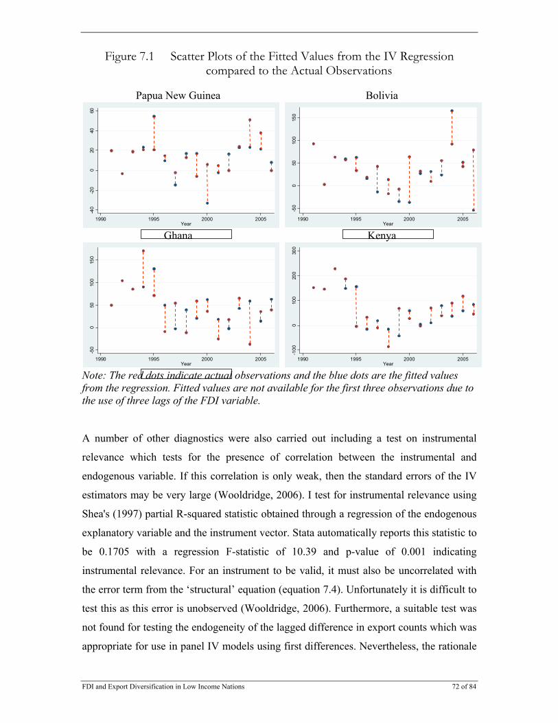
FDI and Export Diversification in Low Income Nations 72 of 84
Figure 7.1 Scatter Plots of the Fitted Values from the IV Regression compared to the Actual Observations
Papua New Guinea
-40
-20
020
4060
1990 1995 2000 2005Year
-40
-20
020
4060
1990 1995 2000 2005Year
Bolivia
-50
050
100
150
1990 1995 2000 2005Year
-50
050
100
150
1990 1995 2000 2005Year
Ghana
-50
050
100
150
1990 1995 2000 2005Year
-50
050
100
150
1990 1995 2000 2005Year
Kenya
-100
010
020
030
0
1990 1995 2000 2005Year
-100
010
020
030
0
1990 1995 2000 2005Year
Note: The red dots indicate actual observations and the blue dots are the fitted values from the regression. Fitted values are not available for the first three observations due to the use of three lags of the FDI variable. A number of other diagnostics were also carried out including a test on instrumental
relevance which tests for the presence of correlation between the instrumental and
endogenous variable. If this correlation is only weak, then the standard errors of the IV
estimators may be very large (Wooldridge, 2006). I test for instrumental relevance using
Shea's (1997) partial R-squared statistic obtained through a regression of the endogenous
explanatory variable and the instrument vector. Stata automatically reports this statistic to
be 0.1705 with a regression F-statistic of 10.39 and p-value of 0.001 indicating
instrumental relevance. For an instrument to be valid, it must also be uncorrelated with
the error term from the ‘structural’ equation (equation 7.4). Unfortunately it is difficult to
test this as this error is unobserved (Wooldridge, 2006). Furthermore, a suitable test was
not found for testing the endogeneity of the lagged difference in export counts which was
appropriate for use in panel IV models using first differences. Nevertheless, the rationale

FDI and Export Diversification in Low Income Nations 73 of 84
for employing the IV technique stemmed from Anderson and Hsiao’s (1981) method
which allowed for the estimation of a dynamic panel model as discussed in section 6.3.
Finally, one of the prime motives for using this model based on first differences was to
control for the non-stationary nature of the data and ensure that regression results were
not spurious. The procedures for testing for unit roots in the residuals of the instrumental
variables and two staged least squares first differenced regression models are in their
infancy and no established tests were found. However, a simpler, less formal technique is
possible. Brooks (2008) suggests that when plotted, stationary residuals would cross their
mean value regularly and not exhibit ‘long swings’ from the mean. Figure 7.2 plots the
residuals from the IV regression for four of the panels over time.
Figure 7.2 Scatter Plots of the IV Regression Residuals
Papua New Guinea
-40
-20
020
40uh
at
1990 1995 2000 2005Year
-40
-20
020
40uh
at
1990 1995 2000 2005Year
Bolivia -1
50-1
00-5
00
5010
0uh
at
1990 1995 2000 2005Year
-150
-100
-50
050
100
uhat
1990 1995 2000 2005Year
Ghana
-100
-50
050
100
uhat
1990 1995 2000 2005Year
-100
-50
050
100
uhat
1990 1995 2000 2005Year
Kenya
-100
-50
050
100
150
uhat
1990 1995 2000 2005Year
-100
-50
050
100
150
uhat
1990 1995 2000 2005Year
Note: These charts were generated using Stata following the regression. The error values are on the vertical axis and the years are along the horizontal axis.

FDI and Export Diversification in Low Income Nations 74 of 84
The residual plots appear to have a mean close to zero and cross this mean value a
number of times indicating no signs of persistence as desired. This indicates that it is
likely that they are well behaved and stationary adding validity to the regression results.
The model was also estimated using the logarithmic values of GDP as an alternate
method of accounting for the scale effects of increasing GDP over time. The coefficients
on the other variables changed little while the coefficient on the exporter’s GDP also
remained negative and statistically insignificant and the coefficient on the importer’s
GDP was positive and statistically significant. Overall the model did not provide any
improvement over the results presented in Table 7.6 and its results are presented in the
appendix (Table 10.2).
7.3 Extensions A number of extensions are possible to this study. Firstly significant improvements can
be made to the quality of the data if it were available. More time periods would improve
the accuracy of the estimation techniques. Furthermore, disaggregated FDI data would
allow for certain types of FDI to be excluded (i.e. investments in the hospitality industry
which may not generate new export channels besides increasing export earning in that
industry). Disaggregated FDI data would also allow for comparing the differences in the
effect of FDI in different industries.
Another noteworthy extension stems from the estimation techniques. The key variable of
interest is in the form of discrete counts and furthermore, it is strictly positive in its levels
form. Estimation techniques which directly address this nature of the data could also be
trailed in future studies. The Tobit model, the Pseudo-Poisson Maximum Likelihood
Estimation Technique and the Negative Binominal technique were considered however
time constraints did not allow for their implementation. Models such as the negative
binomial may also be useful for dealing with the large proportions of zero export flows in
the data.
FDI and Export Diversification in Low Income Nations 75 of 84
A final extension could involve considering different measures of export diversification
as a robustness check. While the count of export channels method employed in this study
may pick up even the slightest change in diversification, it may contain bias towards
certain sectors by its very construction (see discussion in section 5.2). Alternative
methods such as concentration indicis could also be trialled in future studies.

FDI and Export Diversification in Low Income Nations 76 of 84
8 Conclusion and Policy Implications
A number of low income nations have sought to attract increased FDI flows to assist
them in developing new and existing export industries and diversifying their export bases.
In this paper, I have outlined the theoretical case for an association between increased
FDI and export diversification. FDI may result in a direct positive effect on
diversification through the establishment of export platforms while also resulting in
indirect inter and intra-industry spillovers to host nation firms which improve their
productivity and reduce the fixed costs associated with exporting, thereby increasing the
number of firms which are export competitive.
This thesis was then tested empirically using a rich panel dataset comprised of 29 low
income nations and it was found that increases in FDI stock are positively associated with
subsequent increases in export diversification. The bulk of this effect is experienced in
the year that the investment is recorded followed by a drop in diversification in the next
year and an increase in the 2nd and 3rd years after the year that the investment was made.
While it is difficult to isolate the magnitude of the direct and indirect effects of FDI on
these changes in export diversification, the pattern seems consistent with the argument of
FDI resulting in strong direct effects on export diversification in the first year, followed
by spillover benefits in future years. Overall, holding other factors constant, the
cumulative effect after four years of a US$1bn increase in FDI is estimated to be the
creation of 83.5 new export lines.
The findings presented in this paper have a number of potential implications for policy in
low income nations. Firstly, the findings lend some support to government policies which
have aimed to increase FDI flows to help diversify and expand the production and export
bases of low income nations. Secondly, a related point this paper highlights is that the
longer term spillover effects associated with FDI may contribute significantly to its
export diversifying potential. Government policies should thus aim to maximise these
spillovers. Competition should not be restricted, backward linkages should be

FDI and Export Diversification in Low Income Nations 77 of 84
encouraged, and informational spillovers (such as those pertaining to awareness on
foreign market preferences) should be encouraged within the local business community.
The enhancement of such spillovers may assist local businesses in improving their
productivity and learning about foreign markets, potentially helping them to begin
exporting.
Presently, many neighbouring governments are engaged in fierce competition for the
attraction of FDI and many often offer significant incentives such as tax-free periods to
foreign multinationals to win their FDI. This paper sheds some light on the potential
benefits of FDI and governments should carefully consider these benefits when
negotiating to attract FDI, to ensure that the benefits exceed the total costs of any
investment incentives offered. A further significant finding was the importance of free or
preferential trade agreements which were found to have a significantly positive effect on
export diversification.
Finally, another notable point of interest is that for nations which have a high proportion
of oil or mineral exports, the results showed that increased FDI is associated with an
increase in the concentration of the export base. These governments thus face a policy
dilemma in choosing between fostering the development of their resources while also
facing the potential side effects of a more concentrated export base and the ‘Dutch
Disease’ effects discussed in section 3.3. Governments in such nations should potentially
consider investing in promoting a broader variety of FDI opportunities to investors, while
also developing other sectors of their economy, if they are to diversify their exports in the
long term.
FDI and Export Diversification in Low Income Nations 78 of 84
9 References
Aitken, B., Hanson, G. and Harrison, A. 1997. “Spillovers, Foreign Investment, and Export Behaviour”. Journal of International Economics v43, n1-2 : 103-32. Al-Marhubi, F. 2000. “Export Diversification and Growth: An Empirical Investigation”. Applied Economics Letters, 1466-4291, Volume 7, Issue 9, 2000, Pages 559 – 562. Amurgo-Pacheco, A. and Pierola, M. 2008. “Patterns of Export Diversification in Developing Countries: Intensive and Extensive margins”. Policy Research Working Paper Series 4473, the World Bank. Anderson, T. and Hsiao, C. 1981. “Estimation of Dynamic Models with Error Components”. Journal of American Statistical Association, Vol. 76, No. 375, pp. 598-606. Baldwin, R. 2005. “Heterogeneous Firms and Trade: Testable and Untestable Properties of the Melitz Model.” NBER Working Papers, no. 11471. Baltagi, B. 2001. “Econometric Analysis of Panel Data – 2nd Ed”. John Wiley & Sons Ltd. Banga, R. 2003. “The Export Diversifying Impact of Japanese and U.S Foreign Direct Investments in Indian Manufacturing Sector”. ICRIER Working Paper No. 110, September. Baum, C., Schaffer, M., and Stillman, S. 2007. Enhanced Routines for Instrumental Variables/Generalized Method of Moments Estimation and Testing. The Stata Journal (2007) 7, Number 4, pp. 465–506. Bebczuk, R., and Berrettoni, D. 2006. “Explaining Export Diversification: An Empirical Analysis”. CAF Research Program on Development Issues, Department of Economics, Universidad Nacional de La Plata, Argentina. Bernard, A. and Jensen, J. 1999. “Exceptional Exporter Performance: Cause, Effect, or Both?” Journal of International Economics, 47(1): 1–25. Besedes, T. and Prusa, T. 2008. “The Role of Extensive and Intensive Margins and Export Growth”. NBER Working Paper 13628. Blomström, M. and Kokko, A. 1998. “Multinational corporations and spillovers”, Journal of Economic Surveys 12(3): 247-277.

FDI and Export Diversification in Low Income Nations 79 of 84
Bonaglia, F. and Fukasaku, K. 2003. “Export Diversification in Low Income Countries: An International Challenge after Doha”. OECD Development Centre, Working Paper No. 209. Brenton, P. and Newfarmer, R. 2007. “Watching More Than the Discovery Channel: Export Cycles and Diversification in Development”. World Bank Policy Research Working Paper No. 4302. Brooks, C. 2008. “Introductory Econometrics for Finance, Second Edition”. Cambridge University Press. Carrère, C., Strauss-Kahn, V., and Cadot, O. 2007. “Export Diversification: What’s Behind the Hump?” mimeo, Lausanne. Clerides, S., Lach, S. and Tybout, J. 1998. “Is Learning by Exporting Important? Micro-Dynamic Evidence from Colombia, Mexico, and Morocco.” Quarterly Journal of Economics, 113(3): 903-47. Commission on Growth and Development. 2008. “The Growth Report: Strategies for Sustained Growth and Inclusive Development”. < http://www.growthcommission.org> viewed in October 2009. Crespo, N. and Fontoura, M. 2007. “Determinant Factors of FDI Spillovers - What Do We Really Know?” World Development, 35(3): 410-425. Dennis, A. and Shepherd, B. 2007. “Trade Costs, Barriers to Entry, and Export Diversification in Developing Countries”. Policy Research Working Paper No.4368, The World Bank. Dollar, D. and Kraay, A. 2004. “Trade, Growth, and Poverty.” The Economic Journal 114, 22-49. Ekholm, K., Forslid, R., Markusen, J. 2007. “Export-Platform Foreign Direct Investment.” Journal of the European Economic Association 2007 5:4, 776-795. Evenett, S. and Venables, A. 2002. “Export Growth in Developing Countries: Market Entry and Bilateral Trade Flows,” mimeo, London School of Economics. Ferreira, G. 2009. “From Coffee Beans to Microchips: Export Diversification and Economic Growth in Costa Rica.” Southern Agricultural Economics Association - Annual Meeting, January 31-February 3, 2009, Atlanta, Georgia. Freund, C. and Pierola, M. 2008. “Export Surges: The Power of a Competitive Currency.” World Bank, Washington (October). Gorg, H. and Greenaway, D. (2004). “Much Ado About Nothing? Do Domestic Firms Really Benefit From Foreign Direct Investment?” World Bank Research Observer, vol. 19, pp. 171–97.

FDI and Export Diversification in Low Income Nations 80 of 84
Gosh, A. and Ostry, J. 1994. “Export Instability and the External Balance in Developing Countries.” Staff Papers - International Monetary Fund; Jun 1994; 41, 2. Greene, W. 2008. “Econometric Analysis, 6th Ed”. Pearson Prentice Hall. Hausman, J.A. 1978. “Specification Tests in Econometrics.” Econometrica, Vol. 46, No. 6. (Nov., 1978), pp. 1251-1271. Helpman, E. 2006. “Trade, FDI, and the Organization of Firms”. Journal of Economic Literature Vol. XLIV (September 2006), pp. 589–630. Helpman, E., Melitz, M. and Rubinstein, Y. 2006. “Estimating Trade Flows: Trading Partners and Trading Volumes”. Quarterly Journal of Economics, May 2008, Vol. 123, No. 2: 441–487. Herzer, D., and Nowak-Lehmann, F. 2006. “What Does Export Diversification Do for Growth? An Econometric Analysis.” Applied Economics 38: 1825–38. Hesse, H. 2008. “Export Diversification and Economic Growth”. Working Paper, The Commission on Growth and Development. Hopenhayn, H. 1992. “Entry, Exit, and Firm Dynamics in Long Run Equilibrium”. Econometrica 60, 1127–1150. Hummels, D., and Klenow, P. 2005. “The Variety and Quality of a Nation’s Exports,” American Economic Review, 95, 704–719. Im, K., Pesaran, M. and Shin, Y. 2003. “Testing for Unit Roots in Heterogeneous Panels”. Journal of Econometrics, Volume 115, Issue 1, July 2003, Pages 53-74. Imbs, J. and Wacziarg, R. 2003. “Stages of Diversification.” American Economic Review 1993, 63-86. International Trade Centre. 2001. “Kenya’s Export Strategy”. <http://www.intracen.org/wedf/ef2001/kenyapaper1.pdf> viewed in October 2009. Judson, R. and Owen, A. 1997. "Estimating Dynamic Panel Data Models: A Practical Guide for Macroeconomists”. Finance and Economics Discussion Series 1997-3, Board of Governors of the Federal Reserve System (U.S.). Klinger, B. and Lederman, D. 2004. “Discovery and Development: An Empirical Exploration of ‘New’ Products”. World Bank Policy Research Working Paper 3450., World Bank, Washington, D.C. Kokko, A., Tansini, R. and Zejan, M. 1997. “Trade Regimes and Spillover Effects of FDI”. mimeo, Stockholm School of Economics.

FDI and Export Diversification in Low Income Nations 81 of 84
Krugman, P. 1980. “Scale Economies, Product Differentiation, and the Pattern of Trade.” American Economic Review 70, 950–959. Kugler, M. 2005. "Spillovers from Foreign Direct Investment: Within or Between Industries?” Borradores de Economia 369, Banco de la Republica de Colombia. Lederman, D., and Maloney, W. 2007. “Trade Structure and Growth.” In Natural Resources: Neither Curse Nor Destiny, D. Lederman and Maloney W., eds. Palo Alto: Stanford University Press. Markusen, J., and Venables, A. 1999. “Foreign Direct Investment as a Catalyst for Industrial Development.” European Economic Review (43), pp. 335-356. Markusen, J.R. 2000. “Foreign Direct Investment and Trade”, Policy Discussion Paper no. 0019, CIES, University of Adelaide. Melitz, M. 2003. “The Impact of Trade in Intra-Industry Reallocations and Aggregate Industry Productivity”. Econometrica 71(6), 1695-1725. Pesaran, M. 2003. “A Simple Panel Unit Root Test in the Presence of Cross Section Dependence”. Cambridge Working Papers in Economics No. 0346. Rhee, Y. 1990. “The Catalyst Model of Development: Lessons from Bangladesh's Success with Garment Exports”. World Development, Volume 18, Issue 2, Pages 165-346 Rodrígues, E. 1998. “Costa Rica: Policies and Conditions for Export Diversification”. Working Papers No. 154. The UN University, World Institute for Development Economics Research. Sachs, J., and Warner, A. 2000. “Natural Resource Abundance and Economic Growth”. In G.M. Meier and J.E. Rauch (eds), Leading Issues in Economic Development, 7th ed., Oxford University Press, Oxford. Saggi, K. 2002. “Trade, Foreign Direct Investment, and International Technology Transfer: A Survey”. World Bank Research Observer 17, 191-235. Shea, J. 1997. “Instrument Relevance in Multivariate Linear Models: A Simple Measure”. The Review of Economics and Statistics. May 1997, Vol. 79, No. 2, Pages 348-352. de Silva, S., Hadrixo, K. and Tremayne, A. 2009. “Panel Unit Root Tests in the Presence of Cross-sectional Dependence: Finite Sample Performance and an Application”. Econometrics Journal, Volume 12, Issue 2, Date: July 2009, Pages: 340-366. StataCorp. 2001. “Interpreting the Intercept in the Fixed-Effects Model”. Stata Help Website. <http://www.stata.com/support/faqs/stat/xtreg2.html> Viewed in October 2009.
FDI and Export Diversification in Low Income Nations 82 of 84
Wells, L. 1993. “Mobile Exporters: New Foreign Investors in East Asia.” In K.A. Froot, ed., “Foreign Direct Investment”. Chicago: University of Chicago Press. Wooldridge, J. 2006. “Introductory Econometrics: A Modern Approach”. Thompson South-Western. World Bank. 2009. “Strengthening Bolivian Competitiveness: Export Diversification and Inclusive Growth”. Available at <http://go.worldbank.org/MZKWC0MRN0>. Viewed, October 2009.

FDI and Export Diversification in Low Income Nations 83 of 84
10 Appendix
Table 10.1 Levels Model Result – Extended Bilateral Dataset
Coef. P-valuesGDP (Exporter) - Lagged 2.144*** 0.00GDP (Importer) - Lagged 0.008*** 0.00
FDI (Lag1) 6.667*** 0.00FDI (Lag2) -1.533 0.52FDI (Lag3) 1.398 0.60FDI (Lag4) 4.597** 0.03
FDI & High Oil - Lagged -9.671*** 0.00FDI & High Min - Lagged -9.959*** 0.00Exchange Rate -8.598*** 0.00Trade Agreement - Lagged 53.018*** 0.00
North Import Partner 19.796*** 0.00Landlocked -1.867* 0.05Colonial History -10.762** 0.01Common Language 57.516*** 0.00Distance -0.003*** 0.00
1996 -0.090 0.941997 -1.112 0.291998 -4.035*** 0.001999 -4.039*** 0.002000 -3.249** 0.012001 -5.531*** 0.002002 -5.137*** 0.002003 -5.490*** 0.002004 -7.545*** 0.002005 -8.998*** 0.002006 -13.200*** 0.00Constant 19.024** 0.01ObsTWald Chi2Prob > Chi2R-Square (overall)RhoStd. ErrorsFDI Lags Joint Sig. TestTime Dummy Joint Sig. TestPesaran's TestNotes:*** Significant at 1%; ** Significant at 5%; * Significant at 10%All lags are for one period unless otherwise specifiedRobust standard errors are heteroskedasticity consistent
Dependent: Count of Export Channels
1271
P-value: 1.000
P-value: 0.000P-value: 0.000
0.876Robust
0.0000.599
13
Random Effects
7917

FDI and Export Diversification in Low Income Nations 84 of 84
Table 10.2 Differenced Model, Alternate Results – Aggregate Dataset
Dependent: Export Counts (Differenced)
Coef. P-values
Export Counts (Lag 1) 0.725*** 0.00Log GDP (Exporter) -36.151 0.16Log GDP (Importers) 238.040** 0.01
FDI 83.863* 0.06FDI (Lag 1) -49.897 0.20FDI (Lag 2) 1.147 0.96FDI (Lag 3) 44.849 0.13
FDI & High Oil -72.649* 0.09FDI & High Min -98.817** 0.03Exchange Rate 26.695 0.53Trade Agreement 33.329 0.10Constant -7.395 0.15ObsTF-StatProb > FCentered R2Uncentered R2Std. Errors
FDI Lags Joint Sig. TestNotes:*** Significant at 1%; ** Significant at 5%; * Significant at 10%Standard errors are heteroskedasticity and autocorrelation robust
Differenced VariablesIV Regression
37713
40.920.00000.6940.724
HAC Robust, bw=3
P-value: 0.033