Seediscussions,stats,andauthorprofilesforthispublicationat:https://www.researchgate.net/publication/305845613

Forecastingtourismdemandwithcompositesearchindex:

Article·April2017

DOI:10.1016/j.tourman.2016.07.005

CITATION

1

READS

216

4authors,including:

Someoftheauthorsofthispublicationarealsoworkingontheserelatedprojects:

Theimpactofcontextualcuesonresponserate,conversionrate,anddestinationpreferenceintravel

surveysViewproject

BingPan

PennsylvaniaStateUniversity

97PUBLICATIONS3,735CITATIONS

SEEPROFILE

AllcontentfollowingthispagewasuploadedbyBingPanon25August2016.

Theuserhasrequestedenhancementofthedownloadedfile.Allin-textreferencesunderlinedinblueareaddedtotheoriginaldocument

andarelinkedtopublicationsonResearchGate,lettingyouaccessandreadthemimmediately.

Forecasting Tourism Demand with Composite Search Index1

Xin Li, Ph.D.

Institute of Tourism, Beijing Union University

Beijing 100101, China

Email: leexin111@163.com

Bing Pan, Ph.D.

Associate Professor

Department of Hospitality and Tourism Management

School of Business, College of Charleston, Charleston, USA

Email: bingpan@gmail.com

Visiting Professor

School of Tourism and Environmental Sciences

Shaanxi Normal University, Xi’an, China

Rob Law, Ph.D.

Professor

School of Hotel and Tourism Management

The Hong Kong Polytechnic University, Kowloon, Hong Kong

Email: rob.law@polyu.edu.hk

Xiankai Huang, Ph.D.

Professor

Beijing Open University

Beijing 100081, China

Email: xiankai@buu.edu.cn

Submitted Exclusively to Tourism Management

January, 2016

1 This research was partially supported by grants from the National Natural Science Foundation of China (NSFC

No. 71373023 and NSFC No. 41428101) and the Talents Program in Beijing Union University (RK100201509).

Forecasting Tourism Demand with Composite Search Index

Abstract

Researchers have adopted online data such as search query volumes to forecast tourism demand for a

destination, including tourist volumes and hotel occupancy. However, the massive yet highly correlated

query data pose challenges when researchers attempt to include them in the forecasting model. We

propose a framework and procedure for creating a composite search index adopted in a generalized

dynamic factor model (GDFM) to forecast tourist demand in a destination. This research empirically

tests the framework in predicting monthly Beijing tourist volumes. Findings suggest that the proposed

method improves the forecast accuracy of monthly Beijing tourist volumes compared with two

benchmark models: a time series model and a model with an index created by principal component

analysis. The method demonstrates the combination of composite search index and a GDFM in accurately

forecasting tourism demand.

Keywords: tourism demand forecast, big data analytics, search query data, generalized dynamic factor

model, composite search index

1 Introduction

The advancements of the information technology have brought massive amount of big data

generated by users, including search queries, social media mentions, mobile device positions, and

others. (Mayer-Schonberger & Cukier 2013). In particular, search query data provide valuable

information about tourists’ intention, interests, and opinions. Tourists use search engines to obtain

weather and traffic information and to plan their routes by searching for hotels, attractions, travel

guides, and other tourists’ opinions (Fesenmaier, Xiang, Pan, & Law, 2011). Search query data,

including content and volume data, are especially valuable to researchers. They can capture tourists’

attention to travel destinations and can be extremely useful in accurately forecasting tourist volumes

in a destination. The abundant search trends data are favorable sources for tourism forecasting in

the Big Data era. However, they also bring challenges in the modeling process of tourism forecasts.

In particular, in forecasting tourist volumes of one destination with search trends data, one needs to

collect tourism-related keywords, obtain their search trends data, select appropriate data to construct

an aggregated index, and construct the econometric models. The major challenges are keyword

selection and search data aggregation. Keyword selection has received significant attention from

researchers. For example, Brynjolfsson, Geva, and Reichman (2015) proposed a crowd-squared

method to select keywords. They prompted individuals through an online interface to produce word

associations and verified that this method performed efficiently in the keyword selection task. In

addition, the selected search trends data series are usually multi-dimensional, and thus considering

the variables that should be added in the forecast models is important in improving prediction

accuracy.

Compared with keyword selection methods, the process of index aggregation has received limited

attention (Brynjolfsson, Geva, & Reichman, 2015). This step is generally conducted through three

main approaches: (1) incorporating the keywords directly into the models, (2) extracting the index

using the principal component analysis (PCA), and (3) index aggregation from multiple variables

(Yang, Pan, Evans, & Lv, 2015). Although these approaches could predict variables more accurately

than their benchmark models, they are still not optimal. First, multicollinearity or overfitting

problems may occur when the dimensions of variables are high (Varian, 2014). In particular, out-

of-sample forecasts may fail even when in-sample forecasts perform well. Second, a large amount

of the original information will be lost if the data series is weighed equally in aggregating an index

from multiple keywords. The forecast accuracy may be reduced because of incomplete information.

This study aims to propose a feasible variable selection method in forecasting tourist volumes with

search trends data. The approach follows two rules. First, it should acquire one representative and

meaningful index reflecting the dynamic correlation among all search trends data series. Second,

the new method should be able to deal with a large number of search data series. As a result, a

generalized dynamic factor model (GDFM) is adopted to incorporate many keyword variables. An

advantage of GDFM is its ability to process high-dimensional data and to use the composite index

(Amstad & Potter, 2009). GDFM is commonly adopted in the analysis of economic or financial

cycles (Amstad & Potter, 2009), but it is seldom used in the fields of tourism forecasting. We applied

our proposed methodology to predict tourist volumes in Beijing, which is one of the most renowned

travel destinations in China. By collecting specific search trends data from Baidu including tourism-

related keywords (“dining,” “lodging,” “trip,” “traveling,” “shopping,” and “recreation”), this study

empirically tested the method in the forecasting of monthly Beijing tourist volumes from January

2011 to August 2015. The empirical results demonstrate that our method is superior over the

benchmark models of an autoregressive model and a model with PCA as predictor.

This paper proceeds as follows. Section II briefly reviews the relevant literature. Section III proposes

the framework with integrated index construction. Section IV presents our empirical study and

research findings. Finally, Section V concludes by discussing the study’s contributions and

implications for future research.

2 Literature Review

In this section, we first review the current studies on tourism demand forecasting. Second, we focus

on big data forecasting with search trends data, including the major techniques in the keyword and

variable selection. We also introduce the generalized dynamic factor models along with their

applications. Third, we address the research gap at the end of this section.

2.1 Tourism demand forecasting: data and techniques

Tourism demand forecasting is a well-established research area, and it has attracted many studies in

the tourism and hospitality field. Song and Li (2008) gave a detailed literature review on tourist

demand forecasting methods and techniques in recent decades. The commonly adopted forecasting

techniques are time series, econometric models, artificial intelligence approaches, and hybrid

methods.

Time series models predict tourist arrivals by considering past patterns. Many studies used time

series models to analyze and forecast tourism demand (Gunter & Önder, 2015; Guizzardi &

Stacchini, 2015; Akın, 2015; Chu 2009; Chu 2008; Athanasopoulos & Hyndman, 2008). The most

popular ones are autoregressive moving average models (Song & Li, 2008). Econometric models

explore the causal relationship between tourist arrivals and influencing factors, which are especially

useful when a correlational relationship exists (Wong et al., 2007; Wong, Song, & Chon, 2006; Song

& Witt, 2006; Song & Witt, 2000; Song, Witt, & Jensen, 2003). Artificial intelligence methods

adopt neural networks and support vector machines to model the nonlinear data series (Palmer,

Montano, & Sese, 2006; Hadavandi et al., 2015; Pai & Hong, 2005; Pai et al., 2006; Palmer et al.,

2006). Some studies have proposed hybrid forecasting by combining econometric and data mining

techniques (Sun et al., 2016; Pai et al., 2014). In addition, methods such as meta-analysis and

singular spectrum analysis are also used in the modeling and forecasting of tourist arrivals (Hassani

et al., 2015; Peng, Song, & Crouch, 2014).

2.2 Big data analytics in tourism research

Big data analytics has become increasingly important in both the academic and the business

communities over the past two decades (Chen, Chiang, & Storey 2012). Travelers’ decision making

is intrinsically complicated and multi-dimensional, and it includes many aspects such as selecting

destinations, reserving hotels, planning trips, and other activities. The new data sources generated

by users based on Internet technology (search engines or social media platforms) have become

popular in studying travelers’ decision making and behavior.

Some extant literature has attempted to introduce user-generated content and big data analytics in

tourism-related research. With big data sources, tourist arrivals or hotel sales can be forecasted more

accurately. Choi and Varian (2012) investigated the predictive ability of search trends data series in

travel destinations planning. By using keyword search volume data from Google, they increased the

prediction accuracy for Hong Kong tourist arrivals from several countries such as the United States,

Canada, Great Britain, Germany, and other countries. Yang, Pan, and Song (2013) predicted hotel

demand by combining traditional econometric models with web traffic volumes and demonstrated

the use of web volumes in predicting hotel occupancy in a tourist destination.

In addition, these search engine and social media data sources can also help improve customer

service, user experience, and satisfaction (Pan, Litvin, & Goldman, 2006). Ye, Law, and Gu (2009)

examined the effects of online consumer-generated reviews on hotel room sales. The data were

collected from the largest travel website in China. Their research findings indicated a significant

relationship between online reviews and the business performance of hotels. Li, Law, Vu, Rong,

and Zhao (2015) used online reviews data from TripAdvisor to identify emergent hotel features of

interests to international travelers. Their research findings helped hotel managers to gain insights

into travelers’ interests and to better understand rapid changes in tourist preferences. Ghose,

Ipeirotis, and Li (2012) proposed a hotel demand estimation model by combining US hotel

reservation data from Travelocity with various social media sources. They applied big data analytics

such as text mining, image classification, and social geo-tagging to generate a new ranking system

and to provide customers with best-value hotels. Wohlfarth et al. (2011) collected Internet-based

data and used the descriptive characteristics of flights and text mining to predict travel price changes.

The findings help customers to decide when to purchase the best-value tickets. Xiang, Schwartz,

Gerdes Jr., and Uysal (2015) exploited the manner in which big data analytics understands the

relationship between hotel guest experiences and satisfaction. Big data and text analytics can

discover customers’ behavior and represent their experiences.

Compared with traditional data sources in tourism research, big data analytics provides a large

amount of data without sampling bias. With these new data sources, the academia and industries

can better understand consumer behavior in the travel and hospitality fields.

2.3 Forecasting with search trends data

Researchers have adopted search volume data to forecast many social and economic activities. The

forecasted variables include unemployment (Askitas & Zimmermann, 2009), consumption levels

(Swallow & Labbé, 2013; Vosen & Schmidt, 2011), consumer prices (Choi & Varian, 2012),

housing prices (Wu & Brynjolfsson, 2015), and stock prices (Da, Engelberg, & Gao, 2011).

A more recent trend in tourism demand forecasting is forecasting with search trends data from

Google and Baidu. For example, Pan, Wu, and Song (2012) used five travel-related Google search

volume data to predict hotel room demand in an autoregressive moving average with an exogenous

model. Bangwayo-Skeete and Skeete (2015) used Google search and a mixed data sampling model

to improve the forecasting performance of tourist arrivals. Yang et al. (2015) used Baidu and Google

search trends data to predict Chinese tourist flows by using autoregressive moving average models

and evaluated the performances of the data of the two search queries.

In general, researchers use three main data modeling techniques for search volume data. When the

number of relevant search queries is small, researchers include volume data directly in the model

(Vosen & Schmidt, 2011; McLaren, 2011). To accomplish the task, researchers use the

autoregressive moving average with exogenous variables to construct the forecasting model. When

the number of search query data is large, keeping all the variables in the model poses problems

because of potential multicollinearity and overfitting issues in the model estimation (Varian, 2014).

Thus, constructing indices from a large number of search query data is a feasible solution.

Researchers can use PCA to construct a search index (Li, Shang, Wang, & Ma, 2015). In addition,

researchers can aggregate data using data shift and summation in consideration of the lag orders of

different types search query data (Yang, Pan, Evans, & Lv, 2015). Thus, the index is the linear

combination of original search query data series.

The latter two methods create a search index to be included in the forecasting model. In general, the

PCA index is the first factor extracted from the search query data, and the last method is a linear

combination of the partials of the original data. However, both indices may fail to comprehensively

represent the dynamics among all search queries. First, the PCA index is created with the reduction

of the originally high dimensions, thus resulting in information loss in the process. Second, the last

method using shift and summation linearly combines the search queries, and the aggregated index

cannot address the dynamic correlations among search queries. For example, search query data are

dynamically correlated with one another and can be determined by some potentially common factors

such as holidays. Therefore, researchers need a new index construction method to process the multi-

dimensional search queries effectively. The new index should be comprehensive and should reflect

the most relevant information in search queries. It should also depict the common components of

search queries to cover the lead and lag information of the search data series.

2.4 Generalized dynamic factor model

One model seems to be an ideal candidate for modeling multi-dimensional search data. Forni et al.

(2000) proposed GDFM by extending the dynamic factor models. Let , ,{ 1, , 1, }i tx i n t T

be the set of observed variables. Each variable can be modeled as the sum of its common

componenti and an idiosyncratic component

i . The common components are driven by a q-

dimensional vector of common factors'

1 2( , , , )i t t qtf f f f . The model is noted as follows:

( )t t t t tx B L f Eq. 3.1

1 1 2 2( ) ( ) ( )it i t i t iq qtb L f b L f b L f Eq. 3.2

where L is the lag operator, ( ) ( ), 1,2, , , 1,2, ,ijB L b L i n j q is the set of time-varying

factor loadings, and q indicates the number of commonly dynamic factors. Forni et al. (2000)

suggested that q is determined through the variance contribution of each component. If the variance

contribution rate of the first i-1 components diverges and component i begins to converge, then q is

set to i-1. The figure of variance contribution rate is used to determine the value of q. The estimation

details of GDFM are found in Forni et al. (2000) and Forni et al. (2005).

The model has two distinct superiorities in analyzing data with a large number of variables. First,

the model can dynamically update parameters, and thus it can deal with typically dynamic questions.

Second, GDFM allows for cross-correlation among idiosyncratic components. Specifically, GDFM

can generate a coincident index to represent the common states of the observed variables. In the

existing literature, not only can GDFM reflect the business cycle or inflation, but it can also forecast

the dependent variable with cycles. Recently, GDFM has been widely used in the modeling and

forecasting of business cycles (Christophe, 2006), underlying inflation gauges (Amstad & Potter,

2009), and other economic indicators (Forni et al., 2003).

However, the existing literature seldom uses this method to model search trends data in the field of

tourism. The field of tourism is dynamically correlated, and the relevant industrial sectors such as

restaurants, hotels, and travel agencies are also closely correlated with one another. Therefore,

GDFM is an ideal candidate for dealing with multiple tourism-related search trends data series.

3 Methodology

3.1 Forecasting framework with search trends data

After introducing GDFM, we propose a forecasting framework with search trends data. This

framework describes a modeling process that starts from selecting user-generated data sources,

processing data series, and constructing index to building forecasting models and evaluating their

performances. We present the following six steps of this modeling framework:

(I) Select user-generated data sources. Depending on country and culture, different search sources

can be used. For example, several search engines in China such as Baidu and Google can provide

search services for millions of users. In this empirical study, Baidu search trends data are selected

as the major source because Baidu holds the highest market share compared with other search

engines. According to the 35th report issued by the China Internet Network Information Center

(CNNIC, 2015), the Google search engine is less popular in China, with a penetration rate of 27.4%,

which is significantly less than 92.1% of Baidu in 2014.

(II) Select keywords. The purpose of this step is to define tourism-related keywords. This step

intends to follow the mental process of a Chinese traveler who plans to visit a certain city. The

traveler first needs to choose the destination; thereafter, he/she may want to search details about the

food, specialties, traffic, weather, hotels, and insights into the place. Thereafter, we define all of

these aspects, namely, dining, shopping, recreation, lodging, traffic, and insights, as the major

factors that travelers consider in their upcoming trips. The search keywords are selected according

to these aspects.

(III) Process data. This step intends to clean the search trends data series. The data are standardized

to 0–100 to eliminate the influences of scales. The value of 100 indicates the highest search query

volume, and 0 represents the lowest. Moreover, if the data present an extremely high or low point,

then researchers should check the outliers to determine whether the data are affected by one-time

events.

(IV) Construct an index. Through GDFM, a coincident index is constructed to comprehensively

represent a traveler’s interests in a tourist city. This index, which is a combination of the lead and

lag information of all search trends data series, reflects the common components of these search

trends data.

(V) Predict tourist volumes. Several econometric models are constructed and evaluated. In this

research, as a benchmark model, a simple autoregressive moving average model assumes that the

current tourist volumes are influenced by past patterns, and thus it is also considered as a benchmark

model in the existing literature (Song & Li, 2008). Furthermore, we conduct another benchmark

econometric model that obtains the index using PCA. If the GDFM performs the best among the

three models, then we can argue that our method is superior in forecasting tourist volumes.

(VI) Evaluate the forecasting accuracy. To verify the forecasting accuracy of different econometric

models, we adopt three criteria: root mean square error (RMSE), mean absolute error (MAE), and

mean absolute percentage error (MAPE). The model with the lowest values on the three criteria is

the best forecasting model.

1

| | /n

i i

i

MAE y y n

1

100| | /

n

i i i

i

MAPE y y yn

2

1

1( )

n

i i

i

RMSE y yn

.

Select user

genertated data

sources

Select keywords

Process data

Construct index

Predict

Eating Lodging

Traffic Tour

Shopping

Recreation

Forecast actual tourist volumes with

econometric models

Construct index using generalized dynamic

factor model

Clean data using data standardization, outlier

analysis, etc.

Search engines: Baidu, Google, etc.

Search trends data series

Extend

keywords

EvaluateCompare forecast accuracy using RMSE,

MAE, MAPE

I

II

III

IV

V

VI

Fig. 1. Forecasting framework with search trends data

4 Empirical Study

To verify our proposed research framework, we conducted an empirical study on the forecasting of

monthly Beijing tourist volumes. Beijing, the capital of China, is one of the most well-known

destinations attracting a large volume of domestic and international tourists. In this empirical study,

tourist volumes are predicted with Baidu search trends data based on the framework, and the

forecasting accuracies of the different models are evaluated. Section 4.1 describes all data sources

and data correlations. Section 4.2 presents the empirical results.

4.1 Data

4.1.1 Beijing tourist volumes

Monthly Beijing tourist volumes are collected from the Beijing Tourism Association (BJTA, 2015).

The data series, noted as vis, ranges from January 2011 to July 2015. Figure 1 shows the domestic

tourist series in Beijing that presents cyclical fluctuations. For convenient modeling, the logs of

tourist volumes are computed as logvis.

Fig. 1. Monthly Beijing tourist volumes

4.1.2 Baidu search trends data

We take the following steps to select keywords and collect multiple Baidu search trends data to

represent travelers’ interests and search behavior.

1. Six major categories are selected in the aspects of visiting Beijing, namely, dining, lodging,

traffic, tour, shopping, and recreation. These six categories not only reflect the travelers’

demand but also represent relevant industries on the supply side.

2. Several initial keywords in each category are defined using domain knowledge as the seed

keywords. These seeds are used in generating more keywords in the following step.

3. The keyword list is extended using the frequently appearing terms on the search engine

interface; around 200 keywords are obtained. The purpose of this step is to maximize the

possible keyword pool to represent all aspects of tourists’ interests on tourism cities.

4. The abovementioned keywords are checked manually on the Baidu search engine to ensure

the availability of the search trends data series for download. Baidu does not provide search

trends data if the volumes of certain keywords are extremely low. In this process, some

keywords with unavailable volume data are eliminated.

5. The volumes for search trends data series are obtained. These data series represent weekly

frequencies starting from January 1, 2011 to July 25, 2015, as listed in Table 1.

4.1.3 Correlation analysis

Pearson correlations among tourist volumes and all search trends data are computed. Table 1 shows

the contemporaneous correlation coefficients between tourist volumes and search trends data. Most

search trends data are positively correlated with tourist volumes. However, some search trends data

are poorly correlated (e.g., Beijing bar and Beijing recreation places). In existing literature such as

Yang, Pan, Evans, and Lv, (2015), poorly correlated series below a certain threshold are removed.

Different from their approach, our method keeps the search trends data series in our models to

prevent information loss.

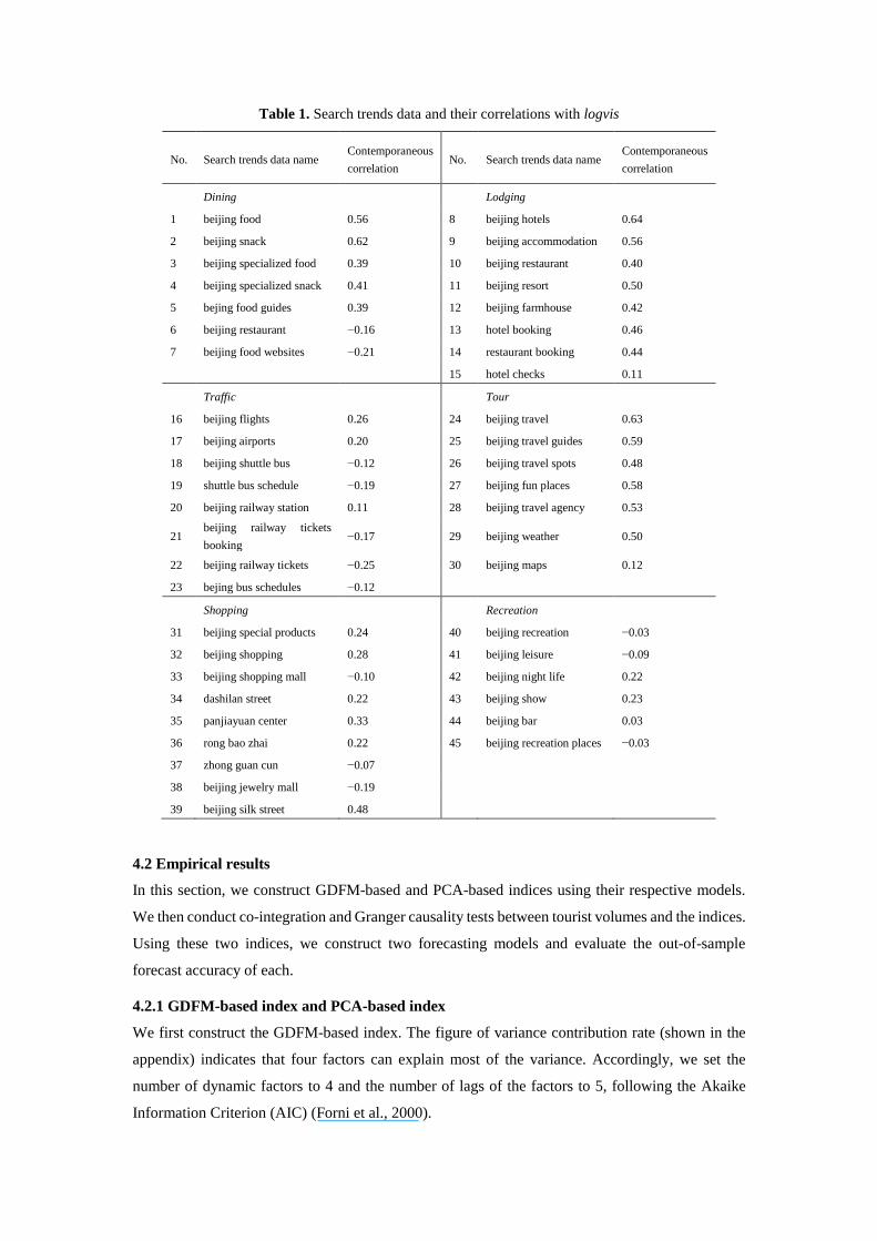
Table 1. Search trends data and their correlations with logvis

No. Search trends data name Contemporaneous

correlation No. Search trends data name

Contemporaneous

correlation

Dining

Lodging

1 beijing food 0.56 8 beijing hotels 0.64

2 beijing snack 0.62 9 beijing accommodation 0.56

3 beijing specialized food 0.39 10 beijing restaurant 0.40

4 beijing specialized snack 0.41 11 beijing resort 0.50

5 bejing food guides 0.39 12 beijing farmhouse 0.42

6 beijing restaurant −0.16 13 hotel booking 0.46

7 beijing food websites −0.21 14 restaurant booking 0.44

15 hotel checks 0.11

Traffic

Tour

16 beijing flights 0.26 24 beijing travel 0.63

17 beijing airports 0.20 25 beijing travel guides 0.59

18 beijing shuttle bus −0.12 26 beijing travel spots 0.48

19 shuttle bus schedule −0.19 27 beijing fun places 0.58

20 beijing railway station 0.11 28 beijing travel agency 0.53

21 beijing railway tickets

booking −0.17 29 beijing weather 0.50

22 beijing railway tickets −0.25 30 beijing maps 0.12

23 bejing bus schedules −0.12

Shopping

Recreation

31 beijing special products 0.24 40 beijing recreation −0.03

32 beijing shopping 0.28 41 beijing leisure −0.09

33 beijing shopping mall −0.10 42 beijing night life 0.22

34 dashilan street 0.22 43 beijing show 0.23

35 panjiayuan center 0.33 44 beijing bar 0.03

36 rong bao zhai 0.22 45 beijing recreation places −0.03

37 zhong guan cun −0.07

38 beijing jewelry mall −0.19

39 beijing silk street 0.48

4.2 Empirical results

In this section, we construct GDFM-based and PCA-based indices using their respective models.

We then conduct co-integration and Granger causality tests between tourist volumes and the indices.

Using these two indices, we construct two forecasting models and evaluate the out-of-sample

forecast accuracy of each.

4.2.1 GDFM-based index and PCA-based index

We first construct the GDFM-based index. The figure of variance contribution rate (shown in the

appendix) indicates that four factors can explain most of the variance. Accordingly, we set the

number of dynamic factors to 4 and the number of lags of the factors to 5, following the Akaike

Information Criterion (AIC) (Forni et al., 2000).

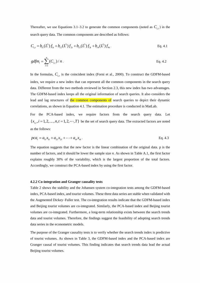
Thereafter, we use Equations 3.1–3.2 to generate the common components (noted as ,i tC ) in the

search query data. The common components are described as follows:

5 5 5 5

, 1 1 2 2 3 3 4 4( ) ( ) ( ) ( )i t i t i t i t i tC b L f b L f b L f b L f . Eq. 4.1

,

1

( ) /n

t i t

i

gdfm C n

. Eq. 4.2

In the formulas, ,i tC is the coincident index (Forni et al., 2000). To construct the GDFM-based

index, we require a new index that can represent all the common components in the search query

data. Different from the two methods reviewed in Section 2.3, this new index has two advantages.

The GDFM-based index keeps all the original information of search queries. It also considers the

lead and lag structures of the common components of search queries to depict their dynamic

correlations, as shown in Equation 4.1. The estimation procedure is conducted in MatLab.

For the PCA-based index, we require factors from the search query data. Let

,{ , 1,2, , , 1,2, , }i tx i n t T be the set of search query data. The extracted factors are noted

as the follows:

1 1 2 2t i t i t ni ntpca a x a x a x . Eq. 4.3

The equation suggests that the new factor is the linear combination of the original data. p is the

number of factors, and it should be lower the sample size n. As shown in Table A.1, the first factor

explains roughly 30% of the variability, which is the largest proportion of the total factors.

Accordingly, we construct the PCA-based index by using the first factor.

4.2.2 Co-integration and Granger causality tests

Table 2 shows the stability and the Johansen system co-integration tests among the GDFM-based

index, PCA-based index, and tourist volumes. These three data series are stable when validated with

the Augmented Dickey–Fuller test. The co-integration results indicate that the GDFM-based index

and Beijing tourist volumes are co-integrated. Similarly, the PCA-based index and Beijing tourist

volumes are co-integrated. Furthermore, a long-term relationship exists between the search trends

data and tourist volumes. Therefore, the findings suggest the feasibility of adopting search trends

data series in the econometric models.

The purpose of the Granger causality tests is to verify whether the search trends index is predictive

of tourist volumes. As shown in Table 3, the GDFM-based index and the PCA-based index are

Granger causal of tourist volumes. This finding indicates that search trends data lead the actual

Beijing tourist volumes.

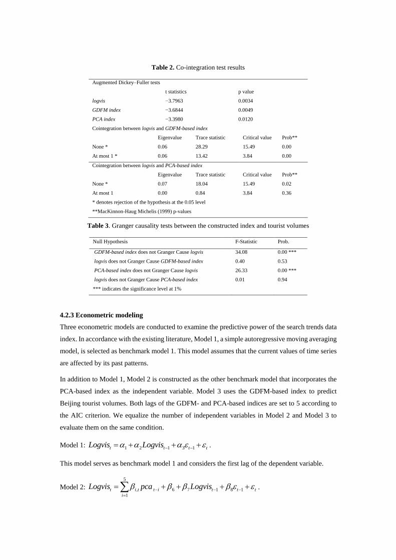
Table 2. Co-integration test results

Augmented Dickey–Fuller tests

t statistics p value

logvis −3.7963 0.0034

GDFM index −3.6844 0.0049

PCA index −3.3980 0.0120

Cointegration between logvis and GDFM-based index

Eigenvalue Trace statistic Critical value Prob**

None * 0.06 28.29 15.49 0.00

At most 1 * 0.06 13.42 3.84 0.00

Cointegration between logvis and PCA-based index

Eigenvalue Trace statistic Critical value Prob**

None * 0.07 18.04 15.49 0.02

At most 1 0.00 0.84 3.84 0.36

* denotes rejection of the hypothesis at the 0.05 level

**MacKinnon-Haug Michelis (1999) p-values

Table 3. Granger causality tests between the constructed index and tourist volumes

Null Hypothesis F-Statistic Prob.

GDFM-based index does not Granger Cause logvis 34.08 0.00 ***

logvis does not Granger Cause GDFM-based index 0.40 0.53

PCA-based index does not Granger Cause logvis 26.33 0.00 ***

logvis does not Granger Cause PCA-based index 0.01 0.94

*** indicates the significance level at 1%

4.2.3 Econometric modeling

Three econometric models are conducted to examine the predictive power of the search trends data

index. In accordance with the existing literature, Model 1, a simple autoregressive moving averaging

model, is selected as benchmark model 1. This model assumes that the current values of time series

are affected by its past patterns.

In addition to Model 1, Model 2 is constructed as the other benchmark model that incorporates the

PCA-based index as the independent variable. Model 3 uses the GDFM-based index to predict

Beijing tourist volumes. Both lags of the GDFM- and PCA-based indices are set to 5 according to

the AIC criterion. We equalize the number of independent variables in Model 2 and Model 3 to

evaluate them on the same condition.

Model 1: 1 2 1 3 1t t t tLogvis Logvis .

This model serves as benchmark model 1 and considers the first lag of the dependent variable.

Model 2:

5

, 6 7 1 8 1

1

t i t t i t t t

i

Logvis pca Logvis

.

In Model 2, the independent variables in Model 1 are retained, and the lags of tpca , which is

computed using Eq. 4.3, are added.

Model 3:

5

, 6 7 1 8 1

1

t i t t i t t t

i

Logvis gdfm Logvis

.

Model 3 incorporates the GDFM-based index obtained from Eq. 4.2. In accordance with Model 2,

the lag of this index is set to 5.

In the abovementioned models, tLogvis indicates the tourist arrivals; 1, 2, 3 indicate the

coefficients of Model 1; and 1 2 8, , , and

1 2 8, , , represent the estimated coefficients of

Models 2 and 3, respectively.

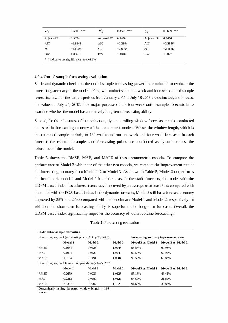
Table 4 presents the estimated coefficients and the key measurements of these three models.

Adjusted R2 describes the fitness of the econometric models, and it is a more valid measurement of

fitness than R2. AIC and SC are information criteria, which also characterize the performance of the

models. The model with the lowest AIC and SC has the best performance. The bolded values in

Table 4 indicate the model with the largest goodness-of-fit and the lowest information criteria.

As shown in Table 4, Model 3 with the GDFM-based index has the highest adjusted R2 and the

lowest AIC and SC criteria. Mode 3 has an adjusted R2 improved by 1.57% and 0.11% compared

with the benchmark and the model with the PCA-based index, respectively.

In terms of the estimated coefficients, all the independent variables are positively correlated with

tourist volumes. In Model 3, a 1% increase in the lags of the GDFM-based index leads to

approximately 0.1% increase in the variance of the dependent variable, with other variables

unchanged. The coefficients of the GDFM-based index in Model 3 are significantly higher than

those in Model 2, thus suggesting that the GDFM-based index contains greater explanatory power

than the PCA-based index.

Table 4. Estimation of econometric models

Model 1 Model 2 Model 3

Variables Coefficients Variables Coefficients Variables Coefficients

1 0.0027 ***

1 0.0206 ***

2 0.0024 ***

2 0.0189 ***

3 0.0023 ***

3 0.0184 ***

4 0.0024 ***

4 0.0191 ***

5 0.0019 ***

5 0.0149 ***

1 7.6943 *** 6 5.9833 ***

6 5.6913 ***

2 0.8829 *** 7 0.9466 ***

7 0.9275 ***

3 0.5008 *** 8 0.3591 ***

8 0.3629 ***

Adjusted R2 0.9334 Adjusted R2 0.9470 Adjusted R2 0.9480

AIC −1.9348 AIC −2.2164 AIC −2.2356

SC −1.8905 SC −2.0964 SC −2.1156

DW 1.8068 DW 1.9010 DW 1.9027

*** indicates the significance level of 1%

4.2.4 Out-of-sample forecasting evaluation

Static and dynamic checks on the out-of-sample forecasting power are conducted to evaluate the

forecasting accuracy of the models. First, we conduct static one-week and four-week out-of-sample

forecasts, in which the sample periods from January 2011 to July 18 2015 are estimated, and forecast

the value on July 25, 2015. The major purpose of the four-week out-of-sample forecasts is to

examine whether the model has a relatively long-term forecasting ability.

Second, for the robustness of the evaluation, dynamic rolling window forecasts are also conducted

to assess the forecasting accuracy of the econometric models. We set the window length, which is

the estimated sample periods, to 180 weeks and run one-week and four-week forecasts. In each

forecast, the estimated samples and forecasting points are considered as dynamic to test the

robustness of the model.

Table 5 shows the RMSE, MAE, and MAPE of these econometric models. To compare the

performance of Model 3 with those of the other two models, we compute the improvement rate of

the forecasting accuracy from Model 1–2 to Model 3. As shown in Table 5, Model 3 outperforms

the benchmark model 1 and Model 2 in all the tests. In the static forecasts, the model with the

GDFM-based index has a forecast accuracy improved by an average of at least 50% compared with

the model with the PCA-based index. In the dynamic forecasts, Model 3 still has a forecast accuracy

improved by 28% and 2.5% compared with the benchmark Model 1 and Model 2, respectively. In

addition, the short-term forecasting ability is superior to the long-term forecasts. Overall, the

GDFM-based index significantly improves the accuracy of tourist volume forecasting.

Table 5. Forecasting evaluation

Static out-of-sample forecasting

Forecasting step = 1 (Forecasting period: July 25, 2015) Forecasting accuracy improvement rate

Model 1 Model 2 Model 3 Model 3 vs. Model 1 Model 3 vs. Model 2

RMSE 0.1084 0.0123 0.0048 95.57% 60.98%

MAE 0.1084 0.0123 0.0048 95.57% 60.98%

MAPE 1.3164 0.1491 0.0584 95.56% 60.83%

Forecasting step = 4 Forecasting periods: July 4–25, 2015

Model 1 Model 2 Model 3 Model 3 vs. Model 1 Model 3 vs. Model 2

RMSE 0.2659 0.0239 0.0128 95.18% 46.42%

MAE 0.2312 0.0180 0.0123 94.68% 31.85%

MAPE 2.8387 0.2207 0.1526 94.62% 30.82%

Dynamically rolling forecast, window length = 180

weeks

Forecasting step = 1 Forecasting accuracy improvement rate

Model 1 Model 2 Model 3 Model 3 vs. Model 1 Model 3 vs. Model 2

RMSE 0.0730 0.0574 0.0566 22.37% 1.27%

MAE 0.0534 0.0435 0.0417 21.91% 4.19%

MAPE 0.6877 0.5645 0.5414 21.28% 4.10%

Forecasting step = 4

Model 1 Model 2 Model 3 Model 3 vs. Model 1 Model 3 vs. Model 2

RMSE 0.2409 0.1626 0.1601 33.55% 1.57%

MAE 0.2009 0.1289 0.1281 36.26% 0.67%

MAPE 2.6068 1.6713 1.6184 37.91% 3.16%

5 Conclusion and Implications

This research proposed a new forecasting framework with search trends data and applied it to the

prediction of Beijing tourist volumes. First, we introduce a GDFM that uses the common

components of search trends data to construct a more comprehensive index. Second, we compare

this new index with a time series model and the PCA-based index model commonly used in existing

studies. We evaluate the performances of the econometric models with different indices using static

and dynamic tests.

The empirical study indicates that our framework has a more favorable performance than other

econometric models. First, a significant co-integration relationship exists between the index and

Beijing tourist volumes. Second, Granger causality tests suggest that search trends data lead the

actual tourist volumes. Third, we demonstrate that the econometric model with the new index has

the best forecasting accuracy in the one-week and four-week forecasts. We also conduct the rolling

window forecasts for the robustness check. The empirical results validated our framework, which

offers a suitable solution for better manipulating large-scale search trends data.

Our research has theoretical implications. We propose a theoretical framework for search trends

data index aggregation based on GDFM. A large dataset of search trends data usually has

complicated correlations. Different from the aggregation in the study of Yang, Pan, Evans, and Lv

(2015), the aggregation of this index is computed through the lead–lag orders among these search

trends data. We compute common components in all search trends data and construct an integrated

index accordingly. The method can better manipulate large datasets of search trends data in a simple

and flexible manner.

Furthermore, timely and accurate tourist forecasts are crucial for policy makers and business

managers. This study indicates that the search trends data index provides more accurate forecasts of

tourist volumes than other indices. Policy makers should monitor this aggregated index to better

capture the dynamics of tourist volumes. In addition, our empirical study demonstrates that this new

index has the best forecasting performance in short-term forecasts. Accurate forecasts can offer

useful support to businesses in making the most strategic decisions during peak or off-peak tourism

seasons.

This research has several limitations, and some of them can be investigated for future research.

Although we expect that the new forecasting framework can be extended to other domains, we still

need further rigorous experiments to examine whether the new methodology can predict other

important indicators in tourism and hospitality such as tourist volumes in other cities, hotel sales,

and flights bookings. We believe that a future study is meaningful when it addresses the importance

of index aggregation in various domains. We hope that this research will encourage future studies

to better process large search trends datasets for more accurate forecasts. Another limitation of this

study is that it mainly focuses on the econometric models with search trends data. In fact, many

effective machine learning approaches are used to model large datasets. Therefore, future studies

should investigate whether our method is useful in nonlinear models.

References

Akın, M. (2015). A novel approach to model selection in tourism demand modeling. Tourism

Management, 48, 64-72.

Amstad, M., & Potter, S. (2009). Real time underlying inflation gauges for monetary policymakers. FRB

of New York Staff Report, (420).

Askitas, N., Zimmermann, K.F., (2009). Google econometrics and unemployment forecasting. Applied

Economics Quarterly, 55, 107–120.

Athanasopoulos, G., & Hyndman, R. J. (2008). Modelling and forecasting Australian domestic tourism.

Tourism Management, 29(1), 19-31.

Bangwayo-Skeete, P. F., & Skeete, R. W. (2015). Can Google data improve the forecasting performance

of tourist arrivals? Mixed-data sampling approach. Tourism Management, 46, 454-464.

Beijing Tourism Association (BJTA), (2015). Beijing Statistical Information Net. Available online

at: http://www.bjstats.gov.cn/sjfb/bssj/jdsj/2015.

Blal, I. & Sturman, M. C. (2014). The differential effects of the quality and quantity of online reviews

on hotel room sales. Cornell Hospitality Quarterly, 55(4), 365-375.

Brynjolfsson, E., Geva, T., & Reichman, S. (2015). Crowd-squared: Amplifying the predictive power of

search trend data. MIS Quarterly (Forthcoming). Available at SSRN:

http://ssrn.com/abstract=2513559.

China Internet Network Information Center (CNNIC). (2015). The penetrate rates of search engines in

China of 2014. The 35th Statistical Report on Internet Development in China (pp: 45-46). Available

online at: https://www.cnnic.cn/hlwfzyj/hlwxzbg/201502/P020150203551802054676.pdf.

Carrière-Swallow, Y., & Labbé, F. (2013). Nowcasting with Google trends in an emerging market.

Journal of Forecasting, 32(4), 289–298.

Chen, H., Chiang Roger, H. L., Storey, V. C. (2012). Business intelligence and analytics: From big data

to big impact. MIS Quarterly, 36(4), 1165-1188.

Choi, H., Varian, H., (2012). Predicting the present with google trends. Economic Record, 88 (s1), 2–9.

Christophe, V. N. (2006). A generalized dynamic factor model for the Belgian economy: Identification

of the business cycle and GDP growth forecasts, National Bank of Belgium Working Papers.

Chu, F. L. (2008). Analyzing and forecasting tourism demand with ARAR algorithm. Tourism

Management, 29(6), 1185-1196.

Chu, F. L. (2009). Forecasting tourism demand with ARMA-based methods. Tourism Management,

30(5), 740-751.

Da, Z., Engelberg, J., & Gao, P., (2011). In search of attention. The Journal of Finance, 66 (5), 1461–

1499.

Fesenmaier, D. R., Xiang, Z., Pan, B., & Law, R. (2011). A framework of search engine use for travel

planning. Journal of Travel Research, 50 (6), 587-601. doi: 10.1177/0047287510385466.

Forni, M., Hallin, M., Lippi, M., & Reichlin, L. (2000). The generalized dynamic-factor model:

Identification and estimation. Review of Economics and Statistics, 82(4), 540-554.

Forni, M., Hallin, M., Lippi, M., & Reichlin, L. (2005). The generalized dynamic factor model. Journal

of the American Statistical Association, 100(471), 830-840.

Forni, M., Hallin, M., Lippi, M., & Reichlin, L. (2003). Do financial variables help forecasting inflation

and real activity in the euro area? Journal of Monetary Economics, 50(6), 1243-1255.

Hadavandi, E., Ghanbarib, A., Shahanaghic, K., & Abbasian-Naghneh, S. (2011). Tourist arrival

forecasting by evolutionary fuzzy systems. Tourism Management, 32(5), 1196-1203.

Hassani, H., Webstera, A., Silvaa, E. S., & Heravic, S. (2015). Forecasting U.S. tourist arrivals using

optimal singular spectrum analysis. Tourism Management, 46, 322-335.

Ghose, A., et al. (2012). Designing ranking systems for hotels on travel search engines by mining user-

generated and crowdsourced content. Marketing Science, 31(3), 493-520.

Guizzardi, A., & Stacchini, A. (2015). Real-time forecasting regional tourism with business sentiment

surveys. Tourism Management, 47, 213-223.

Gunter, U. & Önder, I. (2015). Forecasting international city tourism demand for Paris: Accuracy of uni-

and multivariate models employing monthly data. Tourism Management, 46, 123-135.

Li, G., Law, R., Vu, H. Q., Rong, J., & Zhao, X. R. (2015). Identifying emerging hotel preferences using

Emerging Pattern Mining technique. Tourism Management, 46, 311-321.

Li, X., Shang, W., Wang, S., & Ma, J. (2015). A MIDAS modelling framework for Chinese inflation

index forecast incorporating Google search data. Electronic Commerce Research and Applications,

14(2), 112-125.

Mayer-Schonberger, V., & Cukier, K. (2013). Big data: A revolution that will transform how we live,

work, and think. Eamon Dolan/Houghton Mifflin Harcourt.

McLaren, N. (2011). Using Internet search data as economic indicators. Bank of England Quarterly

Bulletin, 51(2).

Pai, P. F., Huang, K. C., & Lin, K. P. (2014). Tourism demand forecasting using novel hybrid system.

Expert Systems with Applications, 41(8), 3691-3702.

Pai, P. F., & Hong, W. C. (2005). An improved neural network model in forecasting arrivals. Annals of

Tourism Research, 32, 1138-1141.

Pai, P. F., Hong, W. C., Chang, P. T., & Chen, C. T. (2006). The application of support vector machines

to forecast tourist arrivals in Barbados: An empirical study. International Journal of Management,

23, 375-385.

Palmer, A., Montano, J. J., & Sese, A. (2006). Designing an artificial neural network for forecasting

tourism time series. Tourism Management, 27(5), 781-790.

Pan, B., Litvin, S. W., & Goldman, H. (2006). Real users, real trips, and real queries: An analysis of

destination search on a search engine. Annual Conference of Travel and Tourism Research

Association, Dublin, Ireland.

Pan, B., Wu, D. C., & Song, H. (2012). Forecasting hotel room demand using search engine data. Journal

of Hospitality and Tourism Technology, 3(3): 196-210.

Peng, B., Song, H., & Crouch G, I. (2014). A meta-analysis of international tourism demand forecasting

and implications for practice. Tourism Management, 45,181-193.

Song, H., & Li, G., (2008). Tourism demand modelling and forecasting-A review of recent research,

Tourism Management, 29(2): 203–220.

Song, H., & Witt, S. F. (2006). Forecasting international tourist flows to Macau. Tourism Management,

27(2), 214-224.

Song, H., Romilly, P., & Liu, X. (2000). An empirical study of outbound tourism demand in the UK.

Applied Economics, 32, 611-624.

Song, H., Witt, S. F., & Jensen, T. C. (2003). Tourism forecasting: Accuracy of alternative econometric

models. International Journal of Forecasting, 19, 123-141.

Song, H., & Witt, S. (2000). Tourism demand modeling and forecasting: Modern Econometric

Approaches. Oxford: Pergamon Press.

Sun, X., Sun, W., Wang, J., Zhang, Y., & Gao, Y. (2016). Using a Grey–Markov model optimized by

Cuckoo search algorithm to forecast the annual foreign tourist arrivals to China. Tourism

Management, 52, 369-379.

Varian, H. R. (2014). Big data: New tricks for econometrics. Journal of Economic Perspectives, 28(2),

3-27.

Vosen, S., & Schmidt, T. (2011). Forecasting private consumption: survey-based indicators vs. Google

trends. Journal of Forecasting, 30(6), 565-578.

Wong, K. K. F., Song, H., Witt, S, F., & Wu, W. D. C. (2007). Tourism forecasting: To combine or not

to combine? Tourism Management, 28(4), 1068-1078.

Wong, K. K. F., Song, H., & Chon, K. S. (2006). Bayesian models for tourism demand forecasting.

Tourism Management, 27(5), 773-780.

Wohlfarth, T., Clemencon, S., Roueff, F., & Casellato, X. (2011). A data-mining approach to travel price

forecasting. The 10th International Conference on Machine Learning and Applications and

Workshops, 1, 84-89.

Wu, L., & Brynjolfsson, E. (2015). The future of prediction: How Google searches foreshadow housing

prices and sales. In A. Goldfarb, S. M. Greenstein, & C. E. Tucker (1st ed.), Economic Analysis of

the Digital Economy (pp.89-118). Chicago: University of Chicago Press.

Xiang, Z., Wober, K. & Fesenmaier, D. (2008). Representation of the online tourism domain in search

engines. Journal of Travel Research, 47 (2), 137-150.

Xiang, Z., Schwartz, Z., Gerdes Jr J. H., && Uysal, M. (2015). What can big data and text analytics tell

us about hotel guest experience and satisfaction? International Journal of Hospitality Management,

44, 120–130.

Yang, X., Pan, B., Evans, J. A., & Lv, B. (2015). Forecasting Chinese tourist volume with search engine

data. Tourism Management, 46, 386–397.

Ye, Q., Law, R., & Gu, B. (2009). The impact of online user reviews on hotel room sales.

International Journal of Hospitality Management, 28(1), 180–182.

Hamilton, J. D. (1994). Time series analysis (1st ed.). Princeton: Princeton University Press.

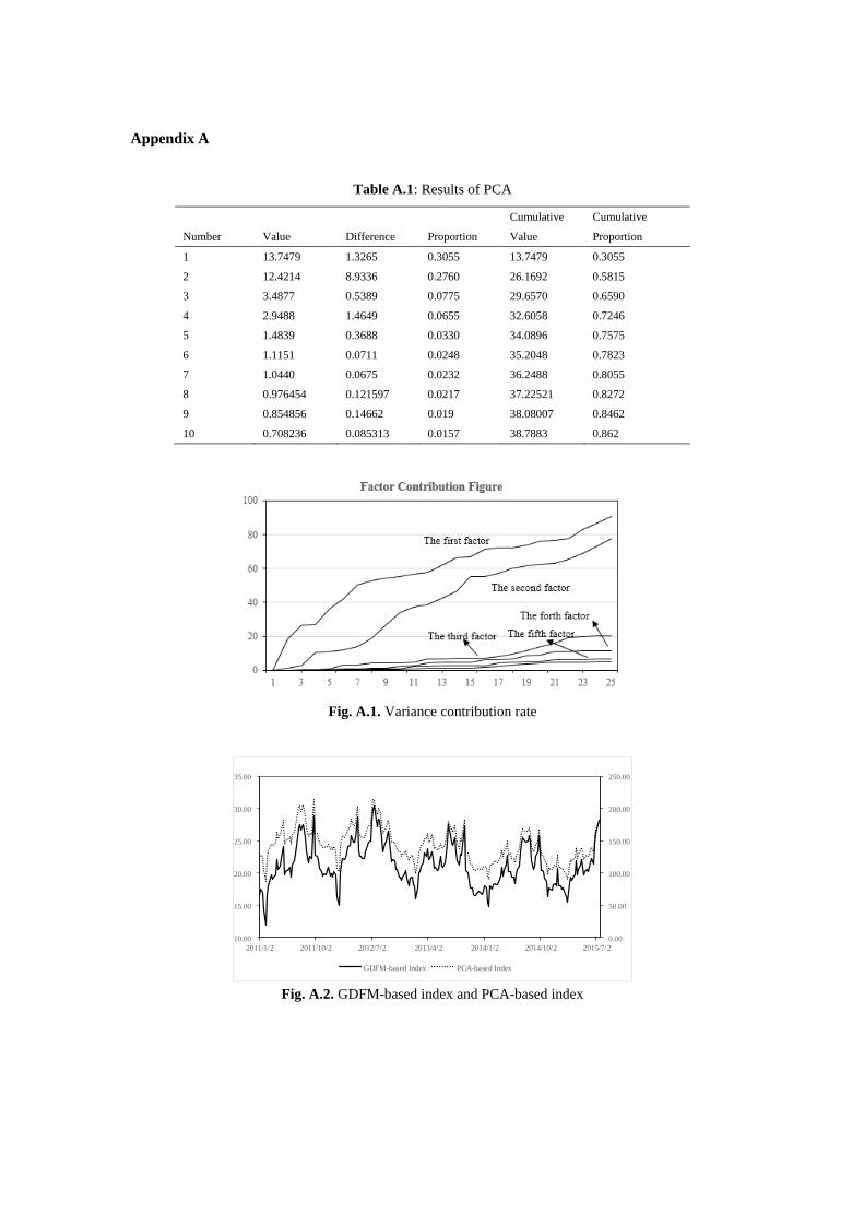
Appendix A

Table A.1: Results of PCA

Cumulative Cumulative

Number Value Difference Proportion Value Proportion

1 13.7479 1.3265 0.3055 13.7479 0.3055

2 12.4214 8.9336 0.2760 26.1692 0.5815

3 3.4877 0.5389 0.0775 29.6570 0.6590

4 2.9488 1.4649 0.0655 32.6058 0.7246

5 1.4839 0.3688 0.0330 34.0896 0.7575

6 1.1151 0.0711 0.0248 35.2048 0.7823

7 1.0440 0.0675 0.0232 36.2488 0.8055

8 0.976454 0.121597 0.0217 37.22521 0.8272

9 0.854856 0.14662 0.019 38.08007 0.8462

10 0.708236 0.085313 0.0157 38.7883 0.862

Fig. A.1. Variance contribution rate

0.00

50.00

100.00

150.00

200.00

250.00

10.00

15.00

20.00

25.00

30.00

35.00

2011/1/2 2011/10/2 2012/7/2 2013/4/2 2014/1/2 2014/10/2 2015/7/2

GDFM-based Index PCA-based Index

Fig. A.2. GDFM-based index and PCA-based index

Author Biography

Xin Li, Ph.D., is a researcher at e-Tourism Research Center, Institute of Tourism,

Beijing Union University. Dr. Li’s research interests are big data analytics, econometric

modeling, data mining and forecasting. Dr. Li focuses on understanding tourism

activities by combing user-generated contents with econometric and machine learning

techniques. She also participated in many research projects on monitoring, forecasting,

and earlywarning of economy and industries in China.

Bing Pan, Ph.D., is an Associate Professor in the Department of Hospitality and

Tourism Management and Head of Research in the Office of Tourism Analysis within

the School of Business at the College of Charleston, USA. His research publications

include using online data to understand, predict, monitor, and forecast tourism

economic activities, tourist online behavior, social media, search engine marketing, and

research methodologies. Dr. Pan has consulted with the Charleston Area Convention

and Visitors Bureau for nine years.

Rob Law, Ph.D., is a Professor at the School of Hotel and Tourism Management, the

Hong Kong Polytechnic University. His research interests are information management,

modelling and forecasting, artificial intelligence and technology applications. He has

received many research related awards and honors, as well as millions of USD external

and internal research grants. Prof. Law serves in different roles for 140+ research

journals, and is a chair/committee member of more than 130 international conferences.

Xiankai Huang, Ph.D., is a Professor at Beijing Open University. Prof. Huang’s

research interests are statistical modeling and tourism forecasting. Prof. Huang has

hosted many national programs such as National Key Technology Research and

Development Program of the Ministry of Science and Technology of China, with over

millions of research grants.

View publication statsView publication stats