3

Forecasting Rubber Production using Intelligent Time Series Analysis

to Support Decision Makers

Panida Subsorn, Dr. Jitian Xiao and Dr. Judy Clayden Edith Cowan University

Australia

1. Introduction

Decision support system (DSS) have become a significant factor for many organisations as

assistive tools for managers to deal with problems (Nakmuang, 2004). Although DSS are

used globally in the agricultural, public, government and especially in business sectors, they

have not been effectively utilised within the public agricultural rubber industry in Thailand.

They assist decision makers to complete decision procedure activities, obtain data,

documents, knowledge or models, increase the number of alternatives examined, achieve

better understanding of the business, provide fast responses to unexpected situations, offer

capability to carry out ad hoc analysis, obtain new insights and learning, facilitate improved

communication, achieve cost savings, achieve better decisions, facilitate more effective

teamwork, achieve time savings and better use of data resources (Keen, 1981; Olson &

Courtney, 1992; Power, 2004; Royal Thai Army, 2007). DSS also present graphical

information and may be integrated with expert systems (ES) and artificial intelligence (AI)

and support both individual and group decision makers (Power, 2004, 2007). Intelligent DSS

demonstrate a range of capabilities and have the capacity to deal with complex data or

problems. Hence, the evolution of intelligent DSS has demonstrated increasing functionality,

including data mining, geographical information systems (GIS), business intelligence (BI),

group DSS (GDSS) and hybrid DSS (Intelligent Science Research Group, 2002; Power, 2007).

These functionalities are applied in intelligent DSS in a wide range of sectors, especially

tourism, agriculture, industry and commerce (Intelligent Science Research Group, 2002;

Power, 2007).

Forecasting, as a significant capability of decision support systems, provides useful

information and supports organizations by facilitating enhanced and desired performance

or management in decision making. Moreover, forecasting is critical within industry

because it enables prediction of future events and conditions by statistically analyzing and

using data or information from the past (Markland & Sweigart, 1987; Tomita, 2007). Results

from forecasting directly affect organizations in the areas of management, planning,

production, sales and prices (Geurts, Lawrence, & Guerard, 1994; Markland & Sweigart,

1987; Olson & Courtney, 1992). Therefore forecasting requires a trustworthy tool to enhance

accuracy before management decisions may be made. Source: Decision Support Systems, Advances in, Book edited by: Ger Devlin,

ISBN 978-953-307-069-8, pp. 342, March 2010, INTECH, Croatia, downloaded from SCIYO.COM

www.intechopen.com

Decision Support Systems, Advances in

44

This chapter examines the use of non-neural network training and neural network training in rubber production forecasting to create a feasible forecasting model for the Thai rubber industry. This chapter is organized as follows: the Thai rubber industry situation is described in Section 2. Section 3 presents the methods which will be used in this study. An experiment is developed by employing non-neural network training and neural network training Techniques in Section 4. Section 5 concludes the paper.

2. The public agricultural rubber industry in Thailand

The agricultural sector has been selected as it is a significant growth sector in Thailand; forecasting may assist in advancing this sector and thereby contribute to Thailand’s economic development. Thailand is the world’s largest rubber exporter to Japan, China and the United States of America with a 39% share of the world market (Office of Industrial Economics & Economic Research and Training Center, 1998; Rubber Research Institute of Thailand, 2007a; Subsorn, 2008). Thailand exports rubber sheet, rubber block, rubber latex and other primary rubber products, whereas only a small fraction of rubber production is reserved for manufacturing within Thailand (Office of Industrial Economics & Economic Research and Training Center, 1998; Rubber Research Institute of Thailand, 2007a; Subsorn, 2008). Production in the public agricultural rubber industry in Thailand is increasing in order to satisfy market demand (Department of Agriculture, 2004). There are several factors related to production, namely seasonal changes, government policy and fluctuations in the global market (Tanguthai & Silpanuruk, 1995). Annual seasonal shifts directly affect rubber production nationally. Between February and September, rubber production decreases because of low levels of rubber latex during the rainy season. However, rubber production increases between October and January because of suitable climatic conditions such as cool climate and no rain (Tanguthai & Silpanuruk, 1995). Government policy is another factor influencing rubber production in Thailand; this relates to supporting agriculturists to produce rubber in order to respond to market demand. The National Economic and Social Development Plan (Issue 10) for Thailand was developed to support agriculturists to respond to market demand, reduce costs and risks in production, gain more income and improve agricultural products and resource management (Office of the National Economic and Social Development Board, 2007). Economic fluctuations directly relate to the global demand for rubber, the market trends and foreign currency exchange (Rubber Research Institute of Thailand, 2007b; Tanguthai & Silpanuruk, 1995). The global demand for rubber is increasing every year, which is the most important factor related to rubber production (Rubber Research Institute of Thailand, 2007b). This global market trend influences forward selling which is important for the marketing and sales of rubber in Thailand (Rubber Research Institute of Thailand, 2007b; Tanguthai & Silpanuruk, 1995). Hence, it is necessary to forecast rubber production in order to know the marketing future so that the industry can respond to the increased demand effectively. Foreign currency exchange directly affects rubber sales (Tanguthai & Silpanuruk, 1995). It influences profit and loss in rubber sales because products in the global market are traded in US dollars. Hence, fluctuations in the US dollar value will also directly affect the Thai Baht value which may positively or negatively affect the Thai economy. In recent years, little attention has been paid to improving production forecasting models or enhancing accuracy in forecasts even though several studies in the Thai rubber industry have focused on management, control and forecasting and have illustrated the need for

www.intechopen.com

Forecasting Rubber Production using Intelligent Time Series Analysis to Support Decision Makers

45

planned development (Leechawengwong, Prathummintra, & Thamsiri, 2002; Subsorn, 2008). However, a focus on improving forecasting is exceptional as this sector has been using the similar models for a long period of time. The existing models apply traditional statistical techniques and may not conduct sufficient tests of validity and reliability of forecasting results. Applying a modern forecasting technique may enhance forecasting results. Thus this chapter attempts to derive a feasible forecasting model for national rubber production in the Thai rubber industry by applying non-neural network training and neural network training techniques. The survival of the current models has created an excellent environment for this study, which aims to create a feasible forecasting model which may provide beneficial additional information for the Thai rubber industry. Results of this chapter may support policy makers in forecasting through its potential to enhance the accuracy of rubber production trends in a competitive environment and reduce losses and risks in development and policy plans.

3. Method

Many existing forecasting methods are differentiated by objectives and/or problems within organizations. Basically, they focus on improvement to gain better performance or to deal with current and future problems. However, some forecasting techniques may not manage particular situations or problems efficiently as they may not be entirely accurate. Hence, this study attempts to gain a feasible forecasting model based on a comparative method and to select a forecasting model which supplies less forecasting errors for this selected sector. In order to provide a better understanding, the following subsections provide a description of non-neural network and neural network Techniques, three main components and data analysis procedures for a feasible new forecasting model for the public agricultural rubber industry in Thailand.

3.1 Non-neural network training and neural network training techniques

i. Non-neural network training technique Time series analysis is often applied in prediction for the component analysis of historical

data sets to determine a forecasting model used to predict the future (Sangpong &

Chaveesuk, 2007). There are several well-known time series forecasting techniques such as

simple moving average (SMA), weight moving average (WMA), exponential smoothing

(ES), seasonal autoregressive integrated moving average (SARIMA). This study deployed

ES and SARIMA techniques for rubber production forecasting. The ES technique has the

capability and efficiency to create trend and seasonal analysis for time series forecasting.

The formula of the ES technique, particularly the simple seasonal exponential smoothing is

as shown below.

( ) ( ( ) ( )) (1 ) ( 1)

( ) ( ( )) (1 ) ( )

ˆ ( ) ( ) ( )t

L t Y t S t s L t

S t Y t S t s

Y k L t S t k s

α α

δ δ

= − − + − −

= + − −

= + + −

(1)

where ˆ ( )tY k is the model-estimated k-step ahead forecasting at time t for series Y, t is the

trend, S is the seasonal length, α is the level smoothing weight and δ is the season

smoothing weight (Statistical Package for the Social Sciences (SPSS), 2009c).

www.intechopen.com

Decision Support Systems, Advances in

46

The SARIMA technique has the capability and efficiency to create seasonal time series

forecasting based on a moving average (MA). Time series data from several consecutive

periods of time are added and divided to obtain mean values to create the prediction

(Sangpong & Chaveesuk, 2007). The formula of the SARIMA technique or equivalent to

autoregressive integrated moving average (ARIMA) (0, 1, (1, s, +1)) (0, 1, 0) with restrictions

among MA parameters is as follows:

( )[ ] ( ) tB y B aµΦ Δ − = Θ 1,...,t N= (2)

where

( ) ( ) ( )

( ) ( ) ( )

p P

q Q

B B B

B B B

ϕ

θ

Φ = Φ

Θ = Θ (3)

where N is the total number of observations, ( 1,2,..., )t t Na = is the white noise series

normally distributed with mean zero and variance 2aσ , p is the order of the non-seasonal

autoregressive part of the model, q is the order of the non-seasonal moving average part of

the model, d is the order of the non-seasonal differencing, P is the order of the seasonal

autoregressive part of the model, Q is the order of the seasonal moving average part of the

model, s it the seasonality or period of the model, ( )p Bϕ is the autoregressive (AR)

polynomial of B of order p, ( )q Bθ is the MA polynomial of B of order q, ( )P BΦ is the

seasonal AR polynomial of BS of order P, ( )Q BΘ is the seasonal MA polynomial of BS of

order Q, Δ is the differencing operator, B is the backward shift operator and µ is the

optional model constant or the stationary series mean. Independent variables x1, x2,…, xm

may be included in the model as the formula is shown below.

1

( ) ( )m

t i it ti

B y c x B aµ=

⎡ ⎤⎛ ⎞Φ Δ − − = Θ⎢ ⎥⎜ ⎟⎜ ⎟⎢ ⎥⎝ ⎠⎣ ⎦∑ (4)

where ci, i = 1,2,..., m is the regression coefficients for the independent variables. ii. Neural network (NN) training technique NN is a well-known predictive technique which claims to provide more reliable results than

other forecasting techniques (Sangpong & Chaveesuk, 2007; Statistical Package for the Social

Sciences (SPSS), 2009a, 2009b). This technique creates the relationship between dependent

and independent variables from several training data sets during the learning process. The

results from this learning process are called neurons. Neurons arrange themselves in a level

form and have connection lines to transfer or process data from input, hidden and output

layers. Each connection line presents weights between each layer connection. Moreover,

neurons adjust their weights via an activation function, which is the processing function to

create the results, to calculate the desirable results (Fausett, 1994; Sangpong & Chaveesuk,

2007). The activation function deployed in this study is the sigmoid function, which is a non-

linear function. Its formula is as shown below.

1

( )1 exp( )

cc

γ =+ −

(5)

www.intechopen.com

Forecasting Rubber Production using Intelligent Time Series Analysis to Support Decision Makers

47

Furthermore, this study employed a supervised learning technique and a feed-forward backpropagation neural network (BPN). Feed-forward BPN were considered to be suitable learning techniques for national rubber production forecasting because of their reliability and accuracy. The supervised learning technique is used to adjust weights for producing forecasting with fewer errors between an output from NN and a desirable output. A feed-forward architecture is the one way connection from input and hidden layers to output layers within the network in the model (Statistical Package for the Social Sciences (SPSS), 2009a). The input layer consists of independent variables or predictors. The hidden layer, consisting of unobservable nodes or units, presents a function to be utilized for independent variables or predictors. The output layer consists of dependent variable(s). Additionally, BPN has the capability to simulate the complicated relationship of the function correctly, which is called an universal approximator, without having knowledge previously of the function relationships (Funahashi, 1989; Hornik, Stinchcombe, & White, 1989; Sangpong & Chaveesuk, 2007). However, overtraining of data sets may cause low efficiency of non-training data sets in the forecasting model. Thus data separation is introduced to solve this problem by dividing the same data set into two groups, namely a training data set and a test data set (Sangpong & Chaveesuk, 2007; Twomey & Smith, 1996). This study partitioned the data set at 70% for the training data set and 30 % for the testing data set. The multilayer perceptron (MLP) was used in this study to facilitate the use of a supervised learning network and a feed-forward BPN. The MLP network is a function of one or many independent variables or predictors in the input layer which may reduce forecasting errors of one or many dependent variables in the output layer (Statistical Package for the Social Sciences (SPSS), 2009b). The MLP formulae are shown below.

Input layer: J0 = P units, a0:1,...,00:Ja with 0: j ja x=

Hidden layer: Ji units, ai:1,..., : ii Ja with ai:k= γj(ci:k) and

1

: : , 1:0

i

a

J

i k i j k i jj

wc−

−=

= ∑ where 1:0 1ia − =

Output layer: JI = R units, aI:1,..., : II Ja with aI:k= γI(cI:k) and

1

: : , 1:0

a

J

I k I j k i jj

wc −=

= ∑ where 1:0 1ia − =

Additionally, an error measurement in the forecasting model used in this study is the root mean square error (RMSE). The formula of this error measurement is shown below.

2ˆ( ( ) ( ))Y t Y t

RMSEn k

−=

−

∑ (6)

where RMSE is the root mean square error values of the forecasting model, Y is the original series of time (t), t is the time series, n is the number of non-missing residuals and k is the number of parameters in the model.

www.intechopen.com

Decision Support Systems, Advances in

48

3.2 Components of the newly refined production forecasting model

This section presents a description of the three main components in the newly refined

forecasting model for national rubber production in the public agricultural rubber industry

in Thailand.

The input component consists of two main subcomponents, namely individual or group

policy makers and input data for forecasting. Policy makers may retrieve or modify

forecasting results via the existing database. Also, they may input new rubber data sets to

create forecasts.

The processing component consists of three main subcomponents, namely time-series

forecasting, artificial intelligence (AI) and error measurement. This study analyses rubber

data sets into two main categories, namely non-neural network training and neural network

training. Then each data set is separately processed using the Statistical Package for the

Social Sciences (SPSS) to create forecasts. Lastly, forecasting errors for accuracy and

reliability purposes are measured with each data set.

The output component consists of two main subcomponents, namely the forecasting results

and the database. The results are produced during the processing component (above). Both

forecasting data sets (non-neural network training and neural network training) are then

compared to the actual corresonding data set. The forecast data is stored in the database for

retrieval and modification for policy makers to make decisions.

3.3 Data analysis process

This chapter used a rubber production data set from the website of the Office of Agricultural

Economics (OAE) in Thailand to examine a newly refined production forecasting model.

The data set was collected on a monthly and yearly basis from the period January 2005 to

December 2008. This chapter focused on national rubber production forecasting. The data

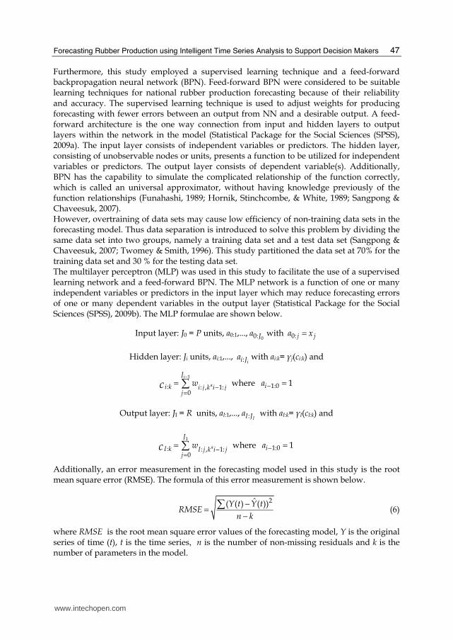
analysis process involved six procedures, as shown in Fig. 1 and described below.

i. Data preparation Time series data from January 2005 to December 2008 was used to prepare a data set for

four months, six months and one year for 2007 and 2008 forecasting. The reason for

selecting forecasting for three different time periods is to enhance validity and

reliability of the newly refined forecasting model.

ii. Sequence chart creation A sequence chart to consider national rubber production trends from January 2005 to

December 2008 was plotted before the forecasts were created. This chart displayed

national rubber production trends to examine a seasonality factor within the trends, so

that suitable forecasting techniques were selected and utilized.

iii. Data processing Non-neural network training and neural network training were used with forecasting

techniques provided in SPSS, namely ES and SARIMA. Analysis involved the use of

these two time-series forecasting techniques for non-neural network training and neural

network training.

iv. Error measurement Errors in the forecasts were examined while SPSS created the forecasts for non-neural network training and neural network training. Forecasting accuracy was thereby strengthened.

www.intechopen.com

Forecasting Rubber Production using Intelligent Time Series Analysis to Support Decision Makers

49

Fig. 1. Data analysis process

v. Comparison of results Forecasting results from non-neural network training and neural network training were compared with the actual prodcution data set for national rubber production to determine the possibility of using this newly refined forecasting model for the public agricultural rubber industry in Thailand.

vi. Creation of figures Figures were created to present forecasting results, comparisons and errors to policy makers and/or decision makers, so that they may have a better understanding or vision before planning and/or making decisions.

The following section presents experimental results, which were compared between non-neural network training and neural network training. Then, the results were classified and presented in four months, six months and one year subsets respectively.

4. Experimental results

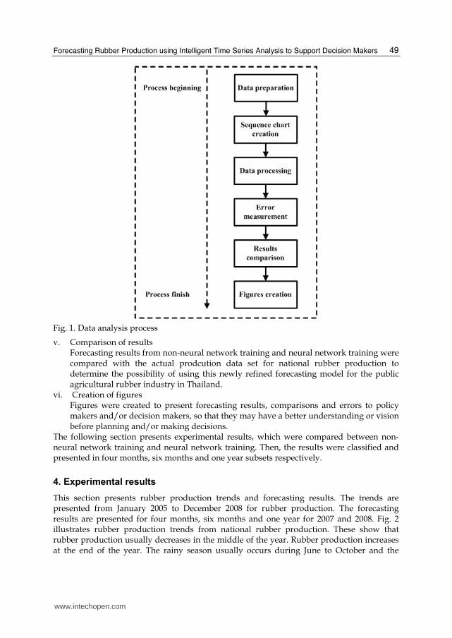
This section presents rubber production trends and forecasting results. The trends are presented from January 2005 to December 2008 for rubber production. The forecasting results are presented for four months, six months and one year for 2007 and 2008. Fig. 2 illustrates rubber production trends from national rubber production. These show that rubber production usually decreases in the middle of the year. Rubber production increases at the end of the year. The rainy season usually occurs during June to October and the

www.intechopen.com

Decision Support Systems, Advances in

50

winter or mild season usually occurs during November to February. Hence, these results confirm that rubber production are related to time-series and seasonality factors.

Fig. 2. National rubber production trend

Fig. 3 and Fig. 4 presents the comparison between the actual national rubber production with non-neural network training and neural network training to identify the best-fitting model in forecasting. Rubber production forecasting results were used with a hold-out sample method to deliver forecasting results validation and evaluation of forecasting accuracy. Rubber production data collected was based upon a hold-out sample method in this section. The following subsections present forecasting results for national rubber production. They were divided into two main subsections as presented below.

4.1 National rubber production forecasts for 2007

The actual rubber production forecasts for 2007 are displayed in Fig. 3 and Tables 1-3, which compare non-neural network training and neural network training with the actual rubber production. It demonstrates that the one year prediction is more successful, for both non-neural network and neural network training techniques, than the four months and the six months predictions. The one year prediction has a root mean square error (RMSE) of 54591.4 for non-neural training and 54261.8 for neural network training. Moreover, the six months prediction is more accurate than the four months prediction. The six months prediction has a RMSE of 56657.4 for non-neural network training and 56141.8 for neural network training. The four months prediction has a RMSE of 57415.8 for non-neural network training and 56847.5 for neural network training. Comparing the RMSE of each model, it is seen that the one year prediction provides the best-fitting forecasting model. Based on this analysis of national rubber production, this demonstrates that the use of neural network training, particularly for three different periods of time, was better than non-neural network training. Non-neural networks are used more

www.intechopen.com

Forecasting Rubber Production using Intelligent Time Series Analysis to Support Decision Makers

51

appropriately when there is data fluctuation which may cause forecasting noise or errors. Moreover, it does not require independent variables in forecasts, unlike neural network forecasting. However, both non-neural network training and neural network training showed similar trends as displayed in the following Fig. 3.

Fig. 3. National rubber production forecasts for 2007

Because it is difficult to show data clearly using graphs, actual figures have been included below in Tables 1-3. The tables include the actual production data and the corresponding predictions using non-neural network training and neural network training predictions respectively.

Date National rubber production

(actual tons) Non-NN training

prediction NN training prediction

Jan-07 351,663 481,562 480,852

Feb-07 245,387 437,861 434,469

Mar-07 159,733 174,706 175,371

Apr-07 157,011 183,331 181,373

May-07 224,145 250,985 246,082

Jun-07 262,923 274,522 271,340

Jul-07 265,593 325,202 328,781

Aug-07 263,391 293,836 293,179

Sep-07 265,564 289,302 287,606

Oct-07 272,872 235,638 237,084

Nov-07 277,741 255,913 255,620

Dec-07 278,184 297,640 299,691

Table 1. One year national rubber prediction

www.intechopen.com

Decision Support Systems, Advances in

52

Date National rubber production

(actual tons) Non-NN training

prediction NN training prediction

Jan-07 351,663 481,562 480,852

Feb-07 245,387 437,861 434,469

Mar-07 159,733 174,706 175,371

Apr-07 157,011 183,331 181,373

May-07 224,145 250,985 246,082

Jun-07 262,923 274,522 271,340

Jul-07 265,593 295,649 300,577

Aug-07 263,391 264,282 264,975

Sep-07 265,564 259,748 259,402

Oct-07 272,872 206,085 208,880

Nov-07 277,741 226,360 227,416

Dec-07 278,184 268,088 271,488

Table 2. Six months national rubber prediction

Date National rubber production

(actual tons) Non-NN training

prediction NN training prediction

Jan-07 351,663 481,562 480,852

Feb-07 245,387 437,861 434,469

Mar-07 159,733 174,706 175,371

Apr-07 157,011 183,331 181,373

May-07 224,145 205,852 200,660

Jun-07 262,923 229,389 225,918

Jul-07 265,593 280,069 283,359

Aug-07 263,391 248,703 247,758

Sep-07 265,564 251,902 249,828

Oct-07 272,872 198,238 199,306

Nov-07 277,741 218,513 217,842

Dec-07 278,184 260,240 261,913

Table 3. Four months national rubber prediction

4.2 National rubber production forecasts for 2008

The actual rubber production forecasts for 2007 are displayed in Fig. 4 and Tables 4-6, which compare non-neural network training and neural network training with the actual rubber production. It demonstrates that the four months prediction is more successful than the six months and the one year predictions. The four months prediction has a RMSE of 52807.5 for non-neural network training and 52020.3 for neural network training. Moreover, the six months prediction is more accurate than the one year prediction.The six months prediction has a root mean square error (RMSE) of 53031.7 for non-neural training and 52254.4 for neural network training. The one year prediction has a RMSE of 53936.8 for non-neural network training and 53398.2 for neural network training. Comparing the RMSE of each model, it is seen that the four months prediction provides the best-fitting forecasting model. Based on this analysis of national rubber production, this

www.intechopen.com

Forecasting Rubber Production using Intelligent Time Series Analysis to Support Decision Makers

53

demonstrates that the use of neural network training, particularly for three different periods of time, was better than non-neural network training. Non-neural networks are used more appropriately when there is data fluctuation which may cause forecasting noise or errors. Moreover, it does not require independent variables in forecasts, unlike neural network forecasting. However, both non-neural network training and neural network training showed similar trends as displayed in the following Fig. 4.

Fig. 4. National rubber production forecasts for 2008

Because it is difficult to show data clearly using graphs, actual figures have been included below in Tables 4-6.

Date National rubber production

(actual tons) Non-NN training

prediction NN training prediction

Jan-08 382,784 436,014 433,865

Feb-08 263,678 371,455 366,969

Mar-08 118,678 167,467 164,537

Apr-08 74,203 172,310 167,664

May-08 215,961 239,791 232,806

Jun-08 251,524 268,409 263,379

Jul-08 287,558 303,085 302,535

Aug-08 317,122 281,440 278,140

Sep-08 338,903 279,142 275,063

Oct-08 369,928 245,802 243,100

Nov-08 281,325 260,942 256,651

Dec-08 381,908 288,908 286,743

Table 4. One year national rubber prediction

www.intechopen.com

Decision Support Systems, Advances in

54

Date National rubber production

(actual tons) Non-NN training

prediction NN training prediction

Jan-08 382,784 436,014 433,865

Feb-08 263,678 371,455 366,969

Mar-08 118,678 167,467 164,537

Apr-08 74,203 172,310 167,664

May-08 215,961 239,791 232,806

Jun-08 251,524 268,409 263,379

Jul-08 287,558 271,688 277,156

Aug-08 317,122 250,043 252,761

Sep-08 338,903 247,745 249,684

Oct-08 369,928 214,405 217,720

Nov-08 281,325 229,545 231,272

Dec-08 381,908 257,510 261,364

Table 5. Six months national rubber prediction

Date National rubber production

(actual tons) Non-NN training

prediction NN training prediction

Jan-08 382,784 436,014 433,865

Feb-08 263,678 371,455 366,969

Mar-08 118,678 167,467 164,537

Apr-08 74,203 172,310 167,664

May-08 215,961 175,572 179,783

Jun-08 251,524 204,190 210,357

Jul-08 287,558 238,867 249,512

Aug-08 317,122 217,223 225,117

Sep-08 338,903 277,217 278,401

Oct-08 369,928 243,877 246,438

Nov-08 281,325 259,017 259,989

Dec-08 381,908 286,983 290,081

Table 6. Four months national rubber prediction

5. Conclusion

This chapter has investigated the best-fitting forecasting model for national rubber production forecasting for 2007 and 2008. The methods used in this study were based on non-neural network training and neural network training techniques to compare with the actual rubber production data for the best-fitting forecasting model. Hence, neural network training was presented to obtain more accurate forecasts for 2007 and 2008. To our knowledge, this is the preliminary study that brings a new perspective to policy makers in the public agricultural rubber industry in Thailand in creating forecasts with AI techniques. This proposed methodology may be considered as a successful decision support tool in national rubber production forecasting in Thailand. It appears that the prediction based on annual production figures is the most likely to be successfully implemented. However, further research over a longer period of time is need to judge more clearly how effectively

www.intechopen.com

Forecasting Rubber Production using Intelligent Time Series Analysis to Support Decision Makers

55

this forecasting model may be applied to the public agricultural rubber industry in Thailand.

6. References

Department of Agriculture. (2004). Academic Rubber Document. Bangkok: Department of Agriculture.

Fausett, L. (1994). Fundamentals of neurla networks: architectures, algorithms, and application. USA: Prentice-Hall.

Funahashi, K. (1989). On the approximate realization of continous mappings by neural networks. Neural networks, 2, 183-192.

Geurts, M., Lawrence, K. D., & Guerard, J. (1994). Forecasting Sales. Greenwich, Connecticut: JAI PRESS INC.

Hornik, K., Stinchcombe, M., & White, H. (1989). Multilayer feedforward networks are universal apprixmators. Neural networks, 2, 359-366.

Intelligent Science Research Group. (2002). Intelligent Decision Support System. Retrieved 6 May 2007, from http://www.intsci.ac.cn/en/research/idss.html

Keen, P. G. W. (1981). Value Analysis: Justifying Decision Support Systems. MIS Quarterly 5(1), 1-16.

Leechawengwong, M., Prathummintra, S., & Thamsiri, Y. (2002). The Development of Basic Rubber Database. Bangkok: Rubber Research Institute of Thailand.

Markland, R. E., & Sweigart, J. R. (1987). Quantitative methods: Applications to managerial decision making. Canada: John Wiley & Sons Inc.

Markland, R. E., & Sweigart, J. R. (1987). Quantitative Methods: Applications to Managerial Decision Making Canada: John Wiley & Sons Inc.

Nakmuang, T. (2004). Decision Support Systems. Retrieved 18 March 2007, from http://www.sirikitdam.egat.com/WEB_MIS/107/index.html

Office of Industrial Economics, & Economic Research and Training Center. (1998). Study of Industrial Structure for Enhancing Competitiveness of Rubber-Product Industries. Bangkok: Ministry of Industry.

Office of the National Economic and Social Development Board. (2007). The National Economic and Social Development Plan Issue 10. Retrieved 29 May, 2007, from http://www.nesdb.go.th/Default.aspx?tabid=139

Olson, D. L., & Courtney, J. F. (1992). Decision Support Models and Expert Systems. New York: Macmillan Publishing Company.

Power, D. J. (2004). Types of Decision Support Systems (DSS). Retrieved 8 April 2007, from http://www.gdrc.org/decision/dss-types.html

Power, D. J. (2007). A Brief History of Decision Support Systems. Retrieved 1 April 2007, from http://dssresources.com/history/dsshistory.html

Royal Thai Army. (2007). Decision Support System. Retrieved 19 March 2007, from http://www.oac.rta.mi.th/.../%BA%B7%B7%D5%E8%2011.doc

Rubber Research Institute of Thailand. (2007a). Academic Rubber Information 2007. Bangkok: Rubber Research Institute of Thailand.

Rubber Research Institute of Thailand. (2007b). Rubber: Price Identifier Factor and Price Guarantee Plan in the Future. Retrieved 29 May, 2007, from http://www.rubberthai.com/newspaper/late_news/2550/May50/main.htm

www.intechopen.com

Decision Support Systems, Advances in

56

Sangpong, S., & Chaveesuk, R. (2007). Time series analysis techniques for forecasting pineapple yield in various sizes. Paper presented at the

ก桜崎ป崎索ชุ肴วิช桜ก桜崎裁渮桜นก桜崎วิ栽錯咲裁ํ桜札นิน採桜น殺ห湮採ช桜載 ิป崎索栽ํ桜ป ๒๕๕๐, Bangkok.

Statistical Package for the Social Sciences (SPSS). (2009a). Introduction to neural networks (Publication. Retrieved 9 June 2009, from Statistical Package for the Social Sciences (SPSS):

Statistical Package for the Social Sciences (SPSS). (2009b). MLP algorithms (Publication. Retrieved 9 June 2009, from Statistical Package for the Social Sciences (SPSS):

Statistical Package for the Social Sciences (SPSS). (2009c). TSMODEL algorithms (Publication. Retrieved 9 June 2009, from Statistical Package for the Social Sciences (SPSS):

Subsorn, P. (2008). Enhancing rubber forecasting: The case of the Thai rubber industry. Paper presented at the Ninth postgraduate electrical engineering & computing symposium (PEECS'2008), The University of Western Australia, Perth, Australia.

Tanguthai, S., & Silpanuruk, K. (1995). Rubber Marketing Management. Songkhla: The Thai Rubber Association.

Tomita, Y. (2007). Introduction to forecasting. Retrieved 8 April 2007, from www.math.jmu.edu/~tomitayx/math328/Ch1Slide.pdf

Twomey, J. M., & Smith, A. E. (1996). Validation and verification. Artificial neural networks for civil engineers: Fundamentals and applications. New York: ASCE Press.

www.intechopen.com

Decision Support Systems Advances inEdited by Ger Devlin

ISBN 978-953-307-069-8Hard cover, 342 pagesPublisher InTechPublished online 01, March, 2010Published in print edition March, 2010

InTech EuropeUniversity Campus STeP Ri Slavka Krautzeka 83/A 51000 Rijeka, Croatia Phone: +385 (51) 770 447 Fax: +385 (51) 686 166www.intechopen.com

InTech ChinaUnit 405, Office Block, Hotel Equatorial Shanghai No.65, Yan An Road (West), Shanghai, 200040, China

Phone: +86-21-62489820 Fax: +86-21-62489821

This book by In-Tech publishing helps the reader understand the power of informed decision making bycovering a broad range of DSS (Decision Support Systems) applications in the fields of medical,environmental, transport and business. The expertise of the chapter writers spans an equally extensivespectrum of researchers from around the globe including universities in Canada, Mexico, Brazil and the UnitedStates, to institutes and universities in Italy, Germany, Poland, France, United Kingdom, Romania, Turkey andIreland to as far east as Malaysia and Singapore and as far north as Finland. Decision Support Systems arenot a new technology but they have evolved and developed with the ever demanding necessity to analyse alarge number of options for decision makers (DM) for specific situations, where there is an increasing level ofuncertainty about the problem at hand and where there is a high impact relative to the correct decisions to bemade. DSS's offer decision makers a more stable solution to solving the semi-structured and unstructuredproblem. This is exactly what the reader will see in this book.

How to referenceIn order to correctly reference this scholarly work, feel free to copy and paste the following:

Panida Subsorn, Jitian Xiao and Judy Clayden (2010). Forecasting Rubber Production Using Intelligent TimeSeries Analysis to Support Decision Makers, Decision Support Systems Advances in, Ger Devlin (Ed.), ISBN:978-953-307-069-8, InTech, Available from: http://www.intechopen.com/books/decision-support-systems-advances-in/forecasting-rubber-production-using-intelligent-time-series-analysis-to-support-decision-makers

© 2010 The Author(s). Licensee IntechOpen. This chapter is distributedunder the terms of the Creative Commons Attribution-NonCommercial-ShareAlike-3.0 License, which permits use, distribution and reproduction fornon-commercial purposes, provided the original is properly cited andderivative works building on this content are distributed under the samelicense.