FORECASTING POLITICAL INSTABILITY: CONTROL … · FORECASTING POLITICAL INSTABILITY:...
61
FORECASTING POLITICAL INSTABILITY: CONTROL-THEORETIC MODELING OF INTERNATIONAL CONFLICT by Brigham Wilson Submitted to Brigham Young University in partial fulfillment of graduation requirements for University Honors Department of Computer Science Brigham Young University August 2010 Advisor: Sean Warnick Signature: Honors Representative: Mike Goodrich Signature:
Transcript of FORECASTING POLITICAL INSTABILITY: CONTROL … · FORECASTING POLITICAL INSTABILITY:...
FORECASTING POLITICAL INSTABILITY:
CONTROL-THEORETIC MODELING OF INTERNATIONAL CONFLICT
by
Brigham Wilson
Submitted to Brigham Young University in partial fulfillment
of graduation requirements for University Honors
Department of Computer Science
Brigham Young University
August 2010
Advisor: Sean Warnick
Signature:
Honors Representative: Mike Goodrich
Signature:

Copyright c© 2010 Brigham Wilson
All Rights Reserved
ABSTRACT
FORECASTING POLITICAL INSTABILITY:
CONTROL-THEORETIC MODELING OF INTERNATIONAL CONFLICT
Brigham Wilson
Department of Computer Science
Bachelor of Science
Forecasting political instability is an important research area because it can
lead to less expensive and more accurate political analysis. This knowledge can
then be used to interpret political behavior and guide policymakers’ decision
processes. The challenge is to create a tractable method that retains political
meaning and preserves enough information of the underlying dynamic system
so as to support the development of predictive models. We first discuss an
external data analysis method that models the complex social system of in-
ternational interactions. Then we describe two internal dynamics models and
create our own model based on consensus protocols that is capable of showing
stable disagreement. We verify this model by simulating the dynamics of the
Israeli-Palestinian Conflict. Our model shows some promise of being an accu-
rate representation of the computation mechanisms underlying complex social
multi-agent systems.
ACKNOWLEDGMENTS
I am very grateful for the teaching and help that made this thesis possible.
Thank you: Sean Warnick, for your two years of support and mentoring,
especially the editing of this thesis; my parents, for everything before and
since; my grandparents, for their faith and confidence in me; my friends in
IDeA Labs, for their insights and friendship; Lauren Woodmansee and Logan
Holman for their review of drafts. Any errors that remain do so despite their
best efforts.
Contents
Table of Contents v
List of Figures vi
List of Tables vii
1 Introduction 11.1 Motivation . . . . . . . . . . . . . . . . . . . . . . . . . . . . . . . . . 21.2 Modeling Approaches . . . . . . . . . . . . . . . . . . . . . . . . . . . 31.3 Modeling Challenges . . . . . . . . . . . . . . . . . . . . . . . . . . . 4
1.3.1 Irreproducibility of Political Events . . . . . . . . . . . . . . . 41.3.2 Agent Subgroup Specification . . . . . . . . . . . . . . . . . . 51.3.3 Difficulty of Application . . . . . . . . . . . . . . . . . . . . . 6
1.4 Contributions of this Work . . . . . . . . . . . . . . . . . . . . . . . . 61.5 Literature Review . . . . . . . . . . . . . . . . . . . . . . . . . . . . . 7
2 External Data Analysis Method 92.1 Background . . . . . . . . . . . . . . . . . . . . . . . . . . . . . . . . 92.2 HSW and the EP Tool . . . . . . . . . . . . . . . . . . . . . . . . . . 10
2.2.1 Method Description . . . . . . . . . . . . . . . . . . . . . . . . 102.2.2 Method Analysis . . . . . . . . . . . . . . . . . . . . . . . . . 11
2.3 Summary . . . . . . . . . . . . . . . . . . . . . . . . . . . . . . . . . 17
3 An Internal Dynamics Model for Consensus Network Problems 183.1 Background . . . . . . . . . . . . . . . . . . . . . . . . . . . . . . . . 183.2 Two Related Modeling Examples . . . . . . . . . . . . . . . . . . . . 19
3.2.1 Operational Net Assessment . . . . . . . . . . . . . . . . . . . 193.2.2 Bueno de Mesquita . . . . . . . . . . . . . . . . . . . . . . . . 20
3.3 Consensus Network Problems . . . . . . . . . . . . . . . . . . . . . . 223.3.1 Basic Construction . . . . . . . . . . . . . . . . . . . . . . . . 223.3.2 Linear Position Dynamic Model . . . . . . . . . . . . . . . . . 253.3.3 Nonlinear Influence Dynamics . . . . . . . . . . . . . . . . . . 273.3.4 Network Hierarchy Structure . . . . . . . . . . . . . . . . . . . 283.3.5 Nested Network Model . . . . . . . . . . . . . . . . . . . . . . 29
v
CONTENTS vi
4 Consensus Simulation 324.1 Model Behavior . . . . . . . . . . . . . . . . . . . . . . . . . . . . . . 324.2 Simulation Graphs and Political Instability . . . . . . . . . . . . . . . 34
4.2.1 Change in Ruling Party . . . . . . . . . . . . . . . . . . . . . 354.2.2 Coalitional Change . . . . . . . . . . . . . . . . . . . . . . . . 364.2.3 Attraction and Bifurcation . . . . . . . . . . . . . . . . . . . . 38
4.3 Case Study: Israeli-Palestinian Conflict . . . . . . . . . . . . . . . . . 394.3.1 Motivation . . . . . . . . . . . . . . . . . . . . . . . . . . . . . 394.3.2 Unique Challenges . . . . . . . . . . . . . . . . . . . . . . . . 404.3.3 Agent Subgroups . . . . . . . . . . . . . . . . . . . . . . . . . 414.3.4 Parameter Table . . . . . . . . . . . . . . . . . . . . . . . . . 414.3.5 Model Verification . . . . . . . . . . . . . . . . . . . . . . . . 41
5 Conclusions 455.1 Further Work . . . . . . . . . . . . . . . . . . . . . . . . . . . . . . . 46
List of Figures
4.1 Example Simulation . . . . . . . . . . . . . . . . . . . . . . . . . . . 344.2 Change in Ruling Party . . . . . . . . . . . . . . . . . . . . . . . . . 354.3 Coalitional Change . . . . . . . . . . . . . . . . . . . . . . . . . . . . 374.4 Attraction and Bifurcation . . . . . . . . . . . . . . . . . . . . . . . . 384.5 Nested Network Model Simulation . . . . . . . . . . . . . . . . . . . . 43
vii
List of Tables
4.1 Agent Parameters . . . . . . . . . . . . . . . . . . . . . . . . . . . . . 42
viii
Chapter 1
Introduction
Political instability can be described as a time period when power and positions
of those in government change enough to upset the status quo. Examples of this
would include an incumbent party being voted out of office, a foreign invasion, or
some other major transfer of power. In democracies, political instability is often
marked only by raging op-ed pieces, localized strikes and marches, and other peaceful
demonstrations. When political instability occurs in countries without established
traditions of peaceful transitions between powerholders (non-democracies especially),
there is an increased risk of violence, government failure, financial loss, and citizen
suffering.
Forecasting political instability is about predicting future situations that will be
marked by the characteristics explained above. The hope of forecasting political in-
stability is that past data will be able to indicate behavior patterns in key political
stakeholders (agents) that will be valid in the future. Examples of possible political
agents include individuals, social groupings, institutions, and nations. Political insta-
bility can be forecasted by simulating how the current political situation will evolve
and how the balances of power will fluctuate over time. Predictions often focus on the
1
1.1 Motivation 2
agents who will have the greatest effect in negotiations and power transfers. Train-
ing a model with past data to see if it properly forecasts what has already occurred
will enable us to become more confident in our results; however, we will still lack a
guarantee that the model will work for some present conflict whose end result is still
unknown.
1.1 Motivation
Forecasting political instability is valuable because it results in accurate analysis and
is less expensive than other policy-analysis efforts. Applying models and simulations
of political interactions can result in a better understanding of how a situation will
evolve and what are the likely outcomes of alternative actions. It is possible for
forecasting results to lead nation states to better understand other strategic agents,
key moments of change, and important areas of influence, allowing them to avoid
costly mistakes. With this knowledge, pressure can be applied by policymakers to
ensure a more peaceful transition of power.
When a political entity is aware of the best option, it is more likely to make
correct decisions; however, if analysis results in inaccurate conclusions, the likeli-
hood of political conflict can increase. Failures in analysis are directly responsible
for some of the most dramatic political conflicts of the past century: Yom-Kippur
War, the Cuban Missile Crisis, the fall of the Berlin Wall, and Weapons of Mass
Destruction in Iraq. Traditional political analysts are susceptible to certain cogni-
tive errors that have contributed to inaccurate conclusions. Intense conflicts, like the
Israeli-Palestinian Conflict, are often colored by emotion, making it difficult for poli-
cymakers to be unbiased. Control-theoretic modeling forecasting political instability
is an attempt to be less prone to group think, primacy effect, recency effect, bounded
1.2 Modeling Approaches 3
rationality, dissonance, attribution theory, prospect theory, rigid standard operating
procedures, and bureaucratic politics by finding the true dynamics of the system. A
data-driven forecasting model can achieve valuable analytical results while avoiding
these cognitive errors if it accurately models the international conflict.
A data-driven forecasting model is also valuable because it can overcome or al-
leviate the challenges of having many qualified, experienced, and capable strategic
analysts. It would also lessen analysts’ physical and moral burdens of making im-
portant decisions with life-and-death consequences [18]. A system that accurately
forecasts political instability would be less expensive than hiring the many strategic
analysts that are currently used.
1.2 Modeling Approaches
This thesis discusses two main theoretical approaches to forecasting political insta-
bility: external data analysis methods and internal dynamics models. External data
analysis methods create artificial mappings between inputs and their associated out-
puts by finding patterns in the data. While this can result in a methodology that
has predictive power, it provides limited insights into how the system actually works.
The results can still be used to adapt inputs to reach a certain output, but the actual
internal dynamics are not revealed and thus, the ability to apply pressure to certain
agents, relationships, or coalitions by policymakers would be limited. Still, if an ex-
ternal data analysis method provides an accurate mapping of inputs to outputs that
can be used to forecast political instability, it would suggest a certain relationship
exists between the two that could be explored using an internal dynamics model.
Internal dynamics models focus on the actual inner structure of the system. A
simple model is created to simulate the behavior of the relevant agents. Multi-agent
1.3 Modeling Challenges 4
systems, which endow each agent who is important to the political situation with the
ability to interact with other agents, are a useful model type. The model’s parameters
are then calibrated to fit the inputs and outputs. This method results in a greater
understanding of the internal dynamics and thus provides insights not only into the
reachability of outputs but control of the system.
The goal of creating an internal dynamics model to forecast political instability
is to discover the symbolic equations that explain the dynamics that are observed in
an international conflict. Similar to how Newton’s Laws can be used to accurately
predict the behavior of mechanical systems, we are trying to use consensus dynamics
to find the “Newton’s Laws” that govern the interactions of political systems. We
use consensus dynamics because these describe how people change their positions on
issues based on whom they interact with.
1.3 Modeling Challenges
In this work, we are addressing a validation problem. It is difficult to validate our
results due to the irreproducibility of political events, agent subgroup specification,
and difficulty of application, even with a well-designed model. While we attempt to
overcome these challenges, these issues represent weaknesses in our work.
1.3.1 Irreproducibility of Political Events
Unlike other modeling applications, the inability to reproduce international conflict
events is an inherent weakness and obstacle to verification. There is no control, no
duplication, and no experimentation. While some similarities between events may ex-
ist, factors such as leadership transitions, alliance shifts, location developments, and
differences in time make each event unique. Due to human memory, even a hypothet-
1.3 Modeling Challenges 5
ically perfect repetition of an event could have a different effect – remembering that
an agent is repeating a certain action can affect the impact of the second occurrence.
1.3.2 Agent Subgroup Specification
Both modeling approaches described in Section 1.2 face the problem of agent subgroup
specification. Which groups matter most and need to be included as agents in the
model needs to be determined. The goal is to find the simplest model that still
describes the behavior of the actual agents fairly well. At any level, there are internal
dynamics that make a more specific agent beneficial and external dynamics that make
a more general agent beneficial (a person could be argued to be too generic and a
country too complex). The goal of aggregation is to separate agents with opposing
viewpoints into different agent subgroups, while incorporating agents with similar
and consequential geography, political loyalties, religious views, and languages into a
coherent subgroup.
Constancy, how much an agent subgroup loses or gains agents, is desirable in order
to simplify the system. The challenge is that agents change position over time and
could move enough to warrant a different subgroup specification. Agent subgroups
should be created in a manner that retains a maximum level of constancy within
subgroups by minimizing drastic agent position changes over time.
System identification can be used to determine the best agent subgroups. A
collection of different agent subgroups is created in accordance with the economic,
political, and cultural characteristics of the system. With data about how the system
actually evolves, a metric is constructed to determine the difference between the
simulated result and the actual result of the international conflict. Using the metric,
the different combinations of groupings are compared, and the best is chosen.
With any model, there is a tradeoff between simplicity and accuracy. An overly
1.4 Contributions of this Work 6
simplistic model may be tractable, but the conclusions may lack predictive power; an
overly complex model may have predictive power, but be intractable. This balance
between simplicity and accuracy can arise in multiple areas, such as agent subgroup
aggregation, variable specification, and parameter designation.
1.3.3 Difficulty of Application
After a model is created, another obstacle exists : those who actually determine
political policy often are not willing to apply an empirical mathematical model for
important policy decisions. Some fear the rigidity, others the lack of control or lack
of accountability; many simply do not trust a system that appears to disregard the
efforts of thousands of hours of training of thousands of researchers and analysts
around the world. This is an important issue because if the model results do not
influence policymakers, then the model is simply an exercise.
1.4 Contributions of this Work
In a search for an underlying law explaining the social system interactions of in-
ternational conflict, this thesis compares two different approaches to modeling. We
develop two models using consensus dynamics for simulating international interaction
dynamics that could lead to political instability: a linear position dynamic model and
a nested network model. Our analysis of the linear position dynamic model addresses
conditions for convergence and stability. The nested network model is created by
incorporating nonlinear influence dynamics (one for intercoalitional influence and an-
other for intracoalitional influence) and a network structure with a two-level hierarchy
to the linear position dynamic model. While the linear and nonlinear components
have been explored previously by [36] and [20], the coupling of these two protocols
1.5 Literature Review 7
with different inter- and intracoalitional influences is new. Using a data set for the
Israeli-Palestinian Conflict, we simulate the negotiation dynamics between 1987 and
the Oslo Accords in 1993 to check the resulting system for predictive power. We
analyze the visualization results for indications of political instability and for agent
behavior that accurately reflect real-life events.
1.5 Literature Review
The models and results presented in this thesis bear strong resemblance to the litera-
ture of recent decades. While the actual equations were developed independently, the
overall concept of the model was based off Bueno de Mesquita’s work [4] [5] [6]. In his
work, Bueno de Mesquita uses four parameters to describe the political behavior of an
agent: influence, salience, firmness, and position. Although our model uses the same
four parameters, our equations that describe how these values evolve are different.
Our model’s basic construction is quite similar to DeGroot’s [11] model, but we add
additional elements to the dynamics of the adjacency matrix. Our model relates to
the consensus work of Chatterjee and Senata [10] and Friedkin and Johnsen [14].
There have been computational modeling projects simulating complex decision-
making processes of large organization and bureaucracies from certain quantifiable
signals by [7] [45] [30] [2] [31] [42] [22]. While our research has a unique focus on
political instability, the negotiation processes of countries is very similar to those
explored in these papers. A number of researchers have tried to represent political
conflict with mathematical models: [38] summarizes the history and predicted future
of quantitative methods based on political science theory used to create accurate
prediction models for international relations.
A summary of basic social and economic network models is presented by Wasser-
1.5 Literature Review 8
man and Faust [47] and more recently by Jackson [25]. Axelrod [3] provides excellent
examples of agent-based models with analysis through computer simulation and we
use the same tool at the end of this thesis. Much of the literature incorporates game
theoretic methods, such as Charness and Jackson [8] and Myerson [34]. Chatterjee,
Dutta, Ray and Sengupta [9] use sequential interactions between agents, while we use
simultaneous interactions. Our influence dynamics are similar to the bounded confi-
dence model used by Hegselmann and Krause [20] to produce opinion fragmentation
and polarization.
The linear position dynamic model we use is quite similar to Ofati-Saber and
Murray’s [36] Protocol A1, but we add terms to account for the other variables in an
international conflict. DeMarzo, Vayanos and Zwiebel [12] present influence dynamics
and position unidimensionality. Our research also relates to the social influence work
by Friedkin and Johnsen [13] and Lopez-Pintado and Watts [28].
Researchers have applied consensus networks to economics and social systems
(Slikker [41], Young [50], Jackson [25],and Lopez-Pintado [27]) and the spread of
epidemics (Moreno [33], Newman [35]). Although focused on other applications, this
thesis is related to other consensus work with similar mathematical formulations
(Tsitsiklis, Bertsekas and Athans [46] and Krause [26]). Lorenz [29] addresses issues
of stability, although in a different manner than done in this thesis.
The rest of the thesis is organized as follows: In Chapter 2, we explore an external
data analysis method created by [23]. In Chapter 3, we describe an internal dynamics
model for consensus network problems, built off the work of [5] and [36] . In Chapter
4, we simulate the nested network model from Chapter 3 to check how well it fits
the literature and real-life events of the Israeli-Palestinian Conflict. Conclusions are
presented in Chapter 5.
Chapter 2
External Data Analysis Method
2.1 Background
External data analysis methods search for patterns in data to associate certain inputs
with their appropriate outputs. In order to accomplish this in this thesis’ problem
domain, rules are created in a manner that incorporates the backgrounds of the
agents involved in the international conflict so that they fit possible theoretical events.
Unless a researcher has an accurate understanding of the cultural, economic, and
political characteristics of the agents, rules can force notions of patterns onto data
(while excluding contradictory data as outliers), instead of extracting information
from data. The following section analyzes in detail an external data analysis method.
After reviewing its basic construction, we indicate areas that may be insufficient for
creating a predictive model.
9
2.2 HSW and the EP Tool 10
2.2 HSW and the EP Tool
Hudson, Shrodt and Whitmer (HSW) developed the Event Patterns Tool (EP Tool), a
database manager and image creator which allows the user to analyze RSS newsfeeds
for certain patterns based on specified actors, actions, and dates. The goal of the EP
tool is to be “a methodology that is capable of preserving the agential basis of social
interaction, capable of analyzing the rules behind such purposive behavior, capable of
tracking multiple agents as they enact rules through behavior directed at one another,
and capable of capturing the evolution of such interaction over time” [24]. Essentially,
the EP Tool reads newsfeeds and reports the frequency of certain event patterns. The
main body of their work applies the EP Tool to the Israeli-Palestinian Conflict.
2.2.1 Method Description
Having created action and agent dictionaries, HSW created a program that deter-
mined what the words appearing in each headline mean in the cultural context of the
international conflict being modeled. Actions are delimited to a list of predetermined
verbs that are divided into categories: verbal cooperation, material cooperation, ver-
bal conflict, and material conflict. The agent dictionary delineates individuals, orga-
nizations, and coalitions from each other by placing them into unique subgroups. In
their analysis, HSW combine all agents into two major coalitions: Israeli and Pales-
tinian. HSW use a counter to see how many times certain agent-verb-agent combina-
tions occur in AP article headlines and displays the occurrences on a histogram. The
purpose of creating these visualizations is to be able to discern certain patterns in the
international conflict. These patterns can indicate when political instability is likely.
The EP Tool serves as a useful visualization method of the Israeli-Palestinian Con-
flict, but is susceptible to certain shortcomings, which are explained in the following
2.2 HSW and the EP Tool 11
subsection.
2.2.2 Method Analysis
Aggregation
HSW’s method of aggregation has several key benefits. First, although the most
active agents in the Israeli-Palestinian Conflict are few, they do not always respond
to stimuli in an exactly reciprocating manner. For example, AIPAC (The American
Israel Public Affairs Committee) could anger Hamas, which, although not willing to
attack the USA, could attack Israel in response. By aggregating AIPAC and Israel,
analysts would appropriately see Hamas’ action as a response to provocation.
Aggregation can have mixed effects on agent subgroup specification. Combining
individual agents into subgroups increases continuity over the transition of leaders
and political parties that are ideologically equal. Aggregation also works well for
accounting for the many different nouns that can be used in reporting a single agent
(Hamas, Gaza City militants, Palestinians, refugees, etc); however, it also places
agents who often have completely opposing viewpoints (Palestinians, the PLO, the
Palestinian Authority, Hamas, Fatah, Islamic Jihad, etc) into the same subgroup.
This also confuses those who have true influence on the decisions and actions pertinent
to the conflict, and those who are simply observers. Agent aggregation results in an
inflated frequency of interactions because instead of rare actions between many agents,
the EP Tool would detect many actions between few agents.
In applying the EP Tool, if all agents are aggregated into two large subgroups,
some important agents are excluded. In the Israeli-Palestinian Conflict, other states
have a major impact in peace negotiations and in major military excursions. Although
they were often the excuse for Arab military invasions, Palestinians were not the main
2.2 HSW and the EP Tool 12
opposing forces in six major wars which involved Israel : the War of Independence
(1948), the Sinai War (1956), the Six-Day War (1967), the Yom Kippur War (1973),
the First Lebanon War (1982), and the Second Lebanon War (2006) [40]. Only in
the smaller, less organized, sporadic, but still deadly, conflicts (such as the First and
Second Intifadas and the recent Gaza War) was the fighting mainly between Israelis
and Palestinians. Since the interactions with other nations have major ramifications
on the conflict, by ignoring the surrounding states as actors, the EP Tool could miss
major cooperation and conflict events.
Rules and Patterns
There is an issue with assigning cause-and-effect relationships between two events
that are reported in the AP headlines for the same time period. Israel may change its
policy, not in response to some outside Palestinian pressure, but simply because after
an election a new political party takes control of the Knesset. This occurred when
Benjamin Netanyahu followed Shimon Peres as Prime Minister in 1996 and instituted
a “tit-for-tat” policy for responses to Palestinian suicide attacks in Israel. Despite the
real cause for change lying within the Israeli-coalition, the EP Tool would categorize
this action as material cooperation and look for a Palestinian provocation causing the
change in policy.
Understanding the agents using this external data analysis method is difficult
because there are many reasons to explain a matching set of inputs and outputs. For
example, during a certain application of the EP Tool, HSW claim that an offering of
peace (an Olive Leaf) was offered in the middle of a “tit-for-tat” sequence. They claim
that this nested pattern took on the meaning of “You have the choice about which of
our actions to reciprocate. You can reciprocate the violence, or you can reciprocate the
peace. And then we will follow suit” [24]. Decreasing control over negotiations seems
2.2 HSW and the EP Tool 13
to conflict with political theory, where agents seek to create incentives for others to act
a certain way – not to give them choices. Three other valid explanations for this nested
behavior are: the agent is trying to confuse the other agents about its intentions; an
agent is trying to appease one party (the international community) by offering peace,
while appeasing another party (their own constituents) by sending aggressive, non-
conciliatory messages; there are different agents with opposing agendas placed within
a single agent subgroup (an error of aggregation).
Combining all events into two broad categories, the EP Tool can be ignorant of
an event’s severity: a Palestinian youth throwing a rock at an IDF soldier could be
treated the same as a Hamas militant firing a rocket at Sderot. Similarly, permanent
changes (new laws, settlement construction, etc) could be treated with equal weight
as temporary changes (military checkpoints, visa restrictions, etc). If the effect of an
event does not disappear unless a canceling event occurs, then it should affect the
position of an agent more than events whose effect diminishes over time. Although the
emotions of the agents in the events may match, the opportunity cost of the culprit
and the damage to the victim can be quite different, and this should be reflected in
the external data analysis method.
Applying the EP Tool to any conflict requires timing and threshold issues to be
properly considered. Some of the EP Tool’s patterns and rules appear to be based
on Western, and not Semitic, cultural norms. For example, in one analysis, the
researchers assume that after a week, each agent has forgotten the others’ actions.
However, “Islamist[s] can be seen to display great patience. The patience is there
for the planning of terrorist operations that can take years to bring to fruition and
with it its sense of vigilance...Islamist adversaries...expect their ‘wars’ to last decades,
or, indeed, however long it takes” [44]. In the Israeli-Palestinian Conflict, an agent
acting after a weeklong pause is not necessarily a provocation, but can easily be in
2.2 HSW and the EP Tool 14
response to an action that occurred more than seven days before.
The application of a week-long window also ignores the intergenerational issues
of the Israeli-Palestinian Conflict. For many of the issues, such as right-of-return,
borders, and citizenship, ancestors’ actions affect descendants. Although occurring
decades later, an action in 1998 could be the direct response to an insult from 1948.
Imposing time lengths for pauses and provocations can lead to innacuracies when
analyzing conflict between groups in the Middle East.
Thresholds are introduced into the HP Tool in order to distinguish background
noise from signals and these are also susceptible to overlooking the true nature of the
agents. HSW designate four Israeli material conflict events in a six day period below
which no signaling would be apparent to the other side; and for the Palestinians, a
threshold of two material conflict events in a six day period. Material cooperation
was rare, so there was no threshold [24]. By this rule, five attacks in six days sends
a signal to the other side, but four attacks in six days does not. In order for these
artificial thresholds to make sense, the Israelis would have to be more sensitive than
the Palestinians so they react sooner and the Palestinians would have to be thicker
skinned, so they need six events in order for them to realize that Israel is attack-
ing. This does not match the history of the Israeli-Palestinian Conflict. Assigning
frequency-time ratios for distinguishing noise from signals is difficult because each
agent in this conflict closely monitors the words and actions of the other side. While
some events are of so little importance that they do not merit a response, there is no
arbitrary number where they become significant.
Data
Although they are readily available, there are challenges to using news headlines as a
data source. HSW assume that since the Israeli-Palestinian dyad has been the focus
2.2 HSW and the EP Tool 15
of sufficient media attention, “the event data are a reasonably accurate description
of the actual behavior in the system”; however, radical ideas are rarely published
in the mainstream media, and undercoverage and stereotypical reporting are not
abnormal [23]. Due to “ownership, the pressure of advertising, the relations among
media, business, and government, and the process of news production,” there can
often be a strong bias in the media [16]. Some criticize modern reporting because
of its dependence on wire sources, which use press releases, easy-to-locate officials,
media handlers and focus only on the same institutions and sources [16]. Media’s role
as a gatekeeper and an agenda setter makes it particularly vulnerable to bias and
suggests that it should not be the trusted metric for forecasting political instability
with an external data analysis method. Herman and Chomsky conclude that media
employees choose stories that conform to acceptable themes because they are too
distracted by the financial attraction to cheap, convenient official sources; they fear
negative responses from groups that might threaten their dominant position; and
they need to satisfy the desires and biases of their advertisers [21]. The idea of media
being objective and balanced is not a safe assumption for HSW’s EP Tool.
Another issue with using AP headlines is duplicity of reporting. The data is passed
through a one-a-day filter in order to eliminate duplicate reports of the same event
by allowing only one instance of any source-event-target combination in a day [24].
While duplicity is a problem that needs to be addressed, the filter HSW implement
leads to a loss of detail and causes three errors. First, if two similar events were to
occur in one day, only one would be counted. Depending on which event-headline
passed the filter, there could be differences in severity and intelligence. The media
could report one group did the attack, but later in the day find out another did it
and correct the report. The new headline would count as another attack, instead of a
correction of the previous event-headline. Second, if an attack were very severe, then
2.2 HSW and the EP Tool 16
there would be multiple headlines about the attack for days afterwards and this filter
will let those pass through and be counted because they were reported on a different
day, even though a new event did not occur. Major conflict and cooperation events
will be counted more than minor conflict and cooperation. Third, ambiguous English
grammar with different word orderings could result in a confusion between the source
agent and target agent of an event.
Not using this filter might correct for the lack of a severity metric. A major event
would receive more coverage and each unique headline would be counted – resulting
in additional counts in the EP Tool. A sensationalized issue may get over-coverage,
but that is the story that gets more public attention and has a greater effect on the
public, causing the event to have a greater impact.
The ideal periods of analysis cover dates that are reported from the same source
with minimal agent morphing. Analysis that looks at a window that required more
than one data source would have different press biases, audiences, agendas, vocabu-
laries, reporting densities, and corporate pressures.
Verbal communication carries heavy significance in Middle Eastern cultures where
symbolic words can begin and end wars. Not only is verbal communication important,
but it is used in a very different way by Semites than by Westerners.
“The adult Arab makes statements which express threats, demands, or inten-
tions, which he does not intend to carry out but which, once uttered, relax
emotional tension, give psychological relief and at the same time reduce the
pressure to engage in any act aimed at realizing the verbalized goal... Once
the intention of doing something is verbalized, this verbal formulation itself
leaves in the mind of the speaker the impression that he has done something
about the issue at hand, which in turn psychologically reduces the importance
of following it up by actually translating the stated intentions into action...
2.3 Summary 17
There is no confusion between words and action, but rather a psychologically
conditioned substitution of intention (especially when it is uttered repeatedly
and exaggeratedly) achieves such importance that the question of whether or
not it is subsequently carried out becomes of minor significance.” [37]
While this can cause confusion and ambiguous interpretations with Westerners, there
should be less misunderstanding between Israeli and Palestinian coalitions.
2.3 Summary
In summary, an external data analysis method would have more success properly
describing the international conflict if it accounted for the severity and evanescence
of each event. Issues of timing and thresholds are also be important. Finally, unique
regional issues related to media bias and communication should be taken into con-
sideration. If these features are accurately accounted for, an external data analysis
method can be expected to more accurately forecast political instability. These issues,
while pertinent to external data analysis methods, are not as critical in the internal
dynamic model described in the following chapter.
Chapter 3
An Internal Dynamics Model for
Consensus Network Problems
3.1 Background
Internal dynamics models seek to represent the inner workings of a complex system
using a simple model. By looking for the actual causal mechanisms in an international
conflict, we hope to accurately forecast political instability. While the external data
analysis methods lack any knowledge of the structure of the system, the internal
dynamics models identify the inputs and outputs and then attempt to identify the
laws that connect them. The goal is to create a mathematical representation that
can be used to gain additional insights into agent behavior and to create accurate
forecasting of events.
Internal dynamics models often are composed of multi-agent systems where agents
are individuals or groups that are conceptualized as decision makers whose choices
depend on their own states and the states of others. This is compatible with rational-
actor theory, which assumes that people weigh benefits to costs before making deci-
18
3.2 Two Related Modeling Examples 19
sions. The goal is to create a model that maps states to decisions so that the system
can be simulated knowing only the current state variables. In contrast to the EP
Tool that is susceptible to inaccuracies in measures of severity, evanescence, tim-
ing and threshold issues, the linear position dynamic model and the nested network
model that are presented in this chapter do not depend on these issues. Nevertheless,
these models will suffer from inaccuracies in the hypothesized agent structure and
interagent dynamics (which we will assume arise from consensus seeking behavior).
After reviewing two examples, this chapter will present the foundational con-
cepts of consensus network problems. Then, we present a linear position dynamic
model. After discussing certain properties of this model, we present nonlinear in-
fluence dynamics and a network hierarchy structure. Finally, these two elements
are incorporated into the linear position dynamic model to create a nested network
model.
3.2 Two Related Modeling Examples
3.2.1 Operational Net Assessment
The first example is when the American military used a straightforward methodology
to explore a system’s internal network structure. The United States Joint Forces
Command (USJFCOM) created the Operational Net Assessment (ONA), which “was
a formal decision-making tool that broke the enemy down into a series of systems
- military, economic, social, political - and created a matrix showing how all those
systems were interrelated and which of the links among the systems were the most
vulnerable” [17]. ONA is a simple system that explains the basic internal structure
of an international conflict [19]. This analysis tool “provides joint force comman-
ders extensive information in advance of a crisis, leading to actionable knowledge
3.2 Two Related Modeling Examples 20
and decision superiority that facilitate the effective application of diplomatic, eco-
nomic, informational, and military power” [48]. With an emphasis on unconventional
warfare, this system is appropriately focused on the type of conflict and dangerous
situations that exist today.
3.2.2 Bueno de Mesquita
For our second example, we describe Bueno de Mesquita’s internal dynamics model
that takes a conflict, extracts a specific question, and predicts what will happen.
He identifies key stakeholders who have influence on the outcome and then predicts
how important leaders will act in the negotiation process. Dismissing the theory of
some disembodied national interest, he models nations as “leaders trying desperately
to stay in power by building coalitions within their selectorate”. They do this by
“buying off cronies in the case of a dictatorship, for example, or producing enough
good works to keep hoi polloi happy in a democracy” [43]. He assumes that the major
players only care about the outcome and who gets credit for the outcome [5].
This method identifies important actors but does not aggregate them into agent
subgroups. Bueno de Mesquita consults experts to find out what each agent wants,
how focused they are, how much influence they have, and how stubborn they are.
He tries to find hidden solutions where leverage could be employed to create friendly
coalitions or to weaken enemy coalitions by properly aligning incentives with a desired
outcome in surprising or overlooked situations.
After determining which agents to include in his model, Bueno de Mesquita assigns
values between 0 and 100 for each agent’s position, influence, salience, and firmness.
The position of an agent is a measure of what outcome the agent wants concerning
a certain issue; the issue is defined on a linear spectrum with two extremes. The
influence of an agent is how much one agent is followed by the other agents. The
3.2 Two Related Modeling Examples 21
salience of an agent is how important the issue is to that agent. The firmness of an
agent is the stubbornness of that agent. Then he sorts the agents according to their
desires and analyzes possible coalitions. Using a game-theoretic simulation, agents’
positions are allowed to change depending on other agents’ positions. This process
is repeated, agents gravitate to equilibrium positions, and the game continues until a
coalition is strong enough to make and implement the decision. In the end, Bueno de
Mesquita reviews possible simulation paths and concludes which is the most probable
outcome.
This method is valuable because it is focused directly on political instability.
By modeling a negotiation process in an international conflict, Bueno de Mesquita is
searching for conditions that will result in a change in the balance of power. Although
there are certain limitations to the complexity that can be addressed (every tangled
conflict must be condensed into a single, independent issue), Bueno de Mesquita
only uses resources that are easily available and which can be verified by applying
the model to past situations, such as news reports, regional publications, and expert
interviews.
Although this method works holistically and, he claims, in practice, there are is-
sues of robustness. If only a small shift at the beginning causes a great change in
the final result, then the initial conditions must be known accurately in order for
the resulting analysis to be useful. Unfortunately, with political issues, there is not
always an easy scale between 0 and 100 that defines each position. Instead, the values
chosen are often arbitrary and they could be varied slightly without being inaccurate.
Although initial conditions are often important, Bueno de Mesquita’s model is espe-
cially susceptible to error because there is no strict definition that specifies agents’
position, influence, salience, or firmness value.
3.3 Consensus Network Problems 22
3.3 Consensus Network Problems
Consensus network problems have attracted attention in recent years with appli-
cations in multiple fields, as specified in Section 1.5. While we use many of the
traditional formulations, terminology, and definitions from the literature, we have
introduced unique variations for the analysis of international conflict. We propose
that political agents change their positions based on other agents they are forced to
interact with due to identity (e.g. being political parties of the same legislative body)
and who they choose to interact with (two groups who have the same position on an
issue). We begin by describing the basic construction of a consensus network problem
and then we present the linear position dynamic model. After presenting nonlinear in-
fluence dynamics and network structure, we add these to the linear position dynamic
model to create the nested network model.
3.3.1 Basic Construction
First, we explain the basic terminology and definitions of a consensus problem net-
work. We borrow heavily from [36].
Let (V,E,A) be a graph of order n. It is described by the set of nodes (agents)
V = [υ1, ..., υn]T , the set of edges E ⊆ V × V , and a weighted adjacency matrix
A = [aij], with nonnegative adjacency elements aij. The node indices belong to a
finite index set I = {1, 2, ..., n}. An edge is denoted by eij = (υi, υj). The adjacency
elements associated with the edges of the graph are positive ( i.e. eij ∈ E ⇔ aij > 0)
and they describe the position and influence dynamics.
The values of aij depend on the values of four variables that are defined for every
agent: position (Pi), influence (Φi), salience (Si), and firmness (Fi). The position of
an agent is a measure of what outcome the agent wants concerning a certain issue.
3.3 Consensus Network Problems 23
The issue is defined on a linear spectrum with two extremes. The influence of an
agent describes how much one agent’s position affects the position of other agents.
The salience of an agent is how important the issue is to that agent. The firmness
of an agent is the stubbornness of that agent. Although people might quantify each
of these parameters slightly differently, we assume that they would agree with the
relative ordering and the dynamics should qualitatively match even if the numeric
values slightly differ. These four parameters are given by:
Pi ∈ R : 0 ≤ Pi ≤ 100, with P = [P1, ..., Pn]T (3.1)
Φi ∈ R : 0 ≤ Φi ≤ 100, with Φ = [Φ1, ...,Φn]T (3.2)
Si ∈ R : 0 ≤ Si < 100, with S = [S1, ..., Sn]T (3.3)
Fi ∈ R : 0 ≤ Fi < 100, with F = [F1, ..., Fn]T (3.4)
We recognize that political systems have varied and complex levels (people can
form agents, factions, parties, coalitions, nations, etc.), but in our model we will focus
on only two methods of aggregation: neighborhoods and coalitions. How agents are
grouped together is important because it affects how agents influence each other
– specifically, neighborhoods will be used in the nonlinear influence dynamics and
coalitions will be used in the inter- and intracoalitional influences.
A neighborhood is defined for each agent as the set of agents whose position
values are within some neighborhood radius ε. For an agent υi, its neighborhood can
be denoted as Ni = {υj ∈ V : |Pi[k]− Pj[k]| < ε}. While neighborhood is defined by
position, a coalition is defined by something different than position that affects how
agents will influence each other.
A coalition, Cj, is defined as a subset of agents that have a unique influence rela-
tionship, no matter what their position may be. A model has w coalitions and the inte-
ger nj is the index of the last agent in a coalition Cj. Thus, the set of agents {υ1, ..., υn}
3.3 Consensus Network Problems 24
can be partitioned to show the coalitions as follows: {υn0 , ..., υn1 , υn1+1, ..., υn2 , ..., υnw},
where {υnj−1+1...υnj} = Cj. By this definition, each agent is in one and only one coali-
tion.
In order to clarify the difference between neighborhood and coalition, consider
political parties within a country. A political party would be a neighborhood and
the country would be a coalition. Two parties in the same country who disagree on
an issue would be in different neighborhoods but the same coalition. Two parties
in different countries who agree on an issue would be in the same neighborhood but
different coalitions.
Two nodes, υi and υj, agree if and only if Pi = Pj. Consensus is achieved when
Pi = Pj ∀ υi, υj ∈ Ci and such a point is called a position agreement value for that
coalition. When the model achieves consensus, we want the position agreement value
to somehow describes the international compromised settlement for a real political
negotiation or interaction on a particular issue (for example, the Oslo Accords, the
Nuclear Non-Proliferation Treaty, the Kyoto Protocol, or the Treaty of Lisbon). This
value can be determined by analyzing official declared agent positions and any nego-
tiated settlements between the key stakeholders in the conflict.
Using the format from social network research in [11] and [36], we will represent
the linear agent position dynamics in the form P [k+ 1] = AP [k], where k = {0, 1, ...}
is the time period. We use discrete time, since even though opinions and positions
are continuous, they are only reported, shared, and acted upon in discrete time.
Every node is connected by an edge to every other node (i.e. aij > 0 ∀i, j). Our
nonlinear influence dynamics are similar to those in [20] and are of the form P [k+1] =
A(P [k], t)P [k]. The adjacency element aij are precisely the weights of this graph A.
These two discrete equations provide the general equation form for our dynamic
systems of equations.
3.3 Consensus Network Problems 25
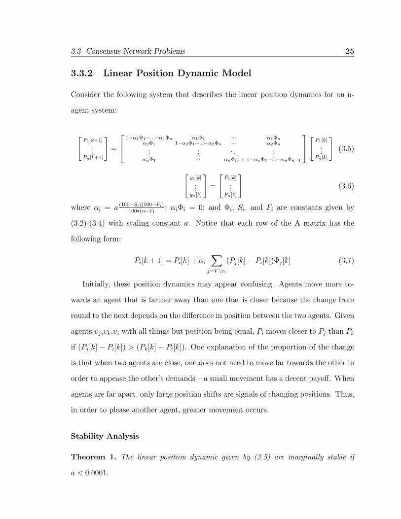
3.3.2 Linear Position Dynamic Model
Consider the following system that describes the linear position dynamics for an n-
agent system:
[P1[k+1]
...Pn[k+1]
]=
1−α1Φ1−...−α1Φn α1Φ2 ··· α1Φnα2Φ1 1−α2Φ1−...−α2Φn ··· α2Φn
......
......
αnΦ1 ··· αnΦn−1 1−αnΦ1−...−αnΦn−1
[P1[k]
...Pn[k]
](3.5)
[y1[k]
...yn[k]
]=
[P1[k]
...Pn[k]
](3.6)
where αi = a (100−Si)(100−Fi)100∗(n−1)
; αiΦi = 0; and Φi, Si, and Fi are constants given by
(3.2)-(3.4) with scaling constant a. Notice that each row of the A matrix has the
following form:
Pi[k + 1] = Pi[k] + αi∑
j=V \υi
(Pj[k]− Pi[k])Φj[k] (3.7)
Initially, these position dynamics may appear confusing. Agents move more to-
wards an agent that is farther away than one that is closer because the change from
round to the next depends on the difference in position between the two agents. Given
agents υj,υk,υi with all things but position being equal, Pi moves closer to Pj than Pk
if (Pj[k]− Pi[k]) > (Pk[k]− Pi[k]). One explanation of the proportion of the change
is that when two agents are close, one does not need to move far towards the other in
order to appease the other’s demands – a small movement has a decent payoff. When
agents are far apart, only large position shifts are signals of changing positions. Thus,
in order to please another agent, greater movement occurs.
Stability Analysis
Theorem 1. The linear position dynamic given by (3.5) are marginally stable if
a < 0.0001.
3.3 Consensus Network Problems 26
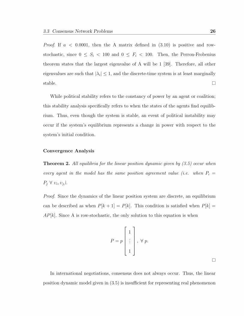
Proof. If a < 0.0001, then the A matrix defined in (3.10) is positive and row-
stochastic, since 0 ≤ Si < 100 and 0 ≤ Fi < 100. Then, the Perron-Frobenius
theorem states that the largest eigenvalue of A will be 1 [39]. Therefore, all other
eigenvalues are such that |λi| ≤ 1, and the discrete-time system is at least marginally
stable.
While political stability refers to the constancy of power by an agent or coalition;
this stability analysis specifically refers to when the states of the agents find equilib-
rium. Thus, even though the system is stable, an event of political instability may
occur if the system’s equilibrium represents a change in power with respect to the
system’s initial condition.
Convergence Analysis
Theorem 2. All equilibria for the linear position dynamic given by (3.5) occur when
every agent in the model has the same position agreement value (i.e. when Pi =
Pj ∀ υi, υj).
Proof. Since the dynamics of the linear position system are discrete, an equilibrium
can be described as when P [k + 1] = P [k]. This condition is satisfied when P [k] =
AP [k]. Since A is row-stochastic, the only solution to this equation is when
P = p
1
...
1
, ∀ p.
In international negotiations, consensus does not always occur. Thus, the linear
position dynamic model given in (3.5) is insufficient for representing real phenomenon
3.3 Consensus Network Problems 27
because it lacks the capability of displaying stable disagreement. This suggests that
we should modify the model. In order to be able to model stable disagreement,
we construct nonlinear influence dynamics that, when implemented in a two-level
hierarchy, will allow for coalitions to have different position agreement values but
also be stable (i.e. PCi[k] 6= PCj
[k] but PCi[k + 1] = PCi
[k] and PCj[k + 1] = PCj
[k]).
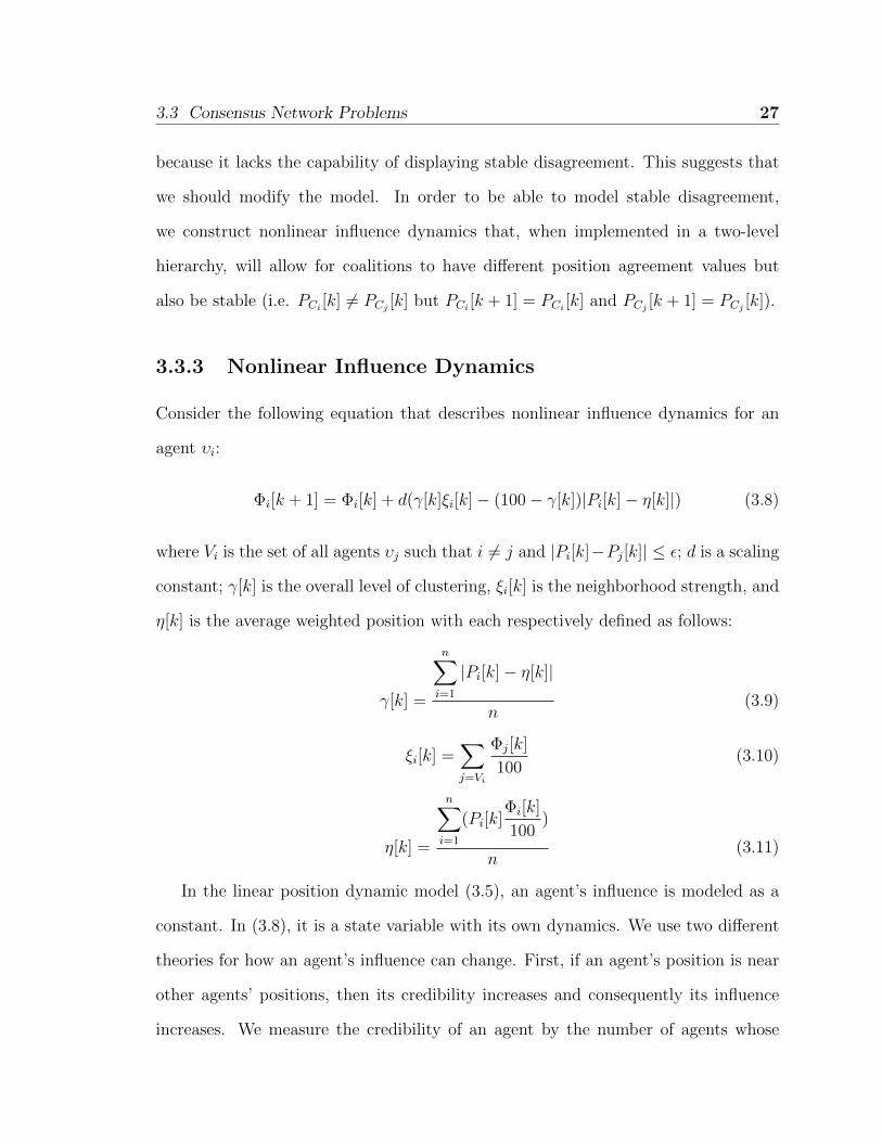
3.3.3 Nonlinear Influence Dynamics
Consider the following equation that describes nonlinear influence dynamics for an
agent υi:
Φi[k + 1] = Φi[k] + d(γ[k]ξi[k]− (100− γ[k])|Pi[k]− η[k]|) (3.8)
where Vi is the set of all agents υj such that i 6= j and |Pi[k]−Pj[k]| ≤ ε; d is a scaling
constant; γ[k] is the overall level of clustering, ξi[k] is the neighborhood strength, and
η[k] is the average weighted position with each respectively defined as follows:
γ[k] =
n∑i=1
|Pi[k]− η[k]|
n(3.9)
ξi[k] =∑j=Vi
Φj[k]
100(3.10)
η[k] =
n∑i=1
(Pi[k]Φi[k]
100)
n(3.11)
In the linear position dynamic model (3.5), an agent’s influence is modeled as a
constant. In (3.8), it is a state variable with its own dynamics. We use two different
theories for how an agent’s influence can change. First, if an agent’s position is near
other agents’ positions, then its credibility increases and consequently its influence
increases. We measure the credibility of an agent by the number of agents whose
3.3 Consensus Network Problems 28
positions are within the neighborhood radius of the agent’s position. Second, since
the average position of all agents is perceived as the most popular position, we decrease
the influence of an agent if it is farther from this average position.
The variance of all of the agents’ positions determines the magnitude of the impact
of the two theories on an agent’s influence. Using a measure of clustering (γ[k]) to
describe the level of variance, we construct a convex combination to incorporate these
two elements: if there is a high level of clustering (γ[k]), the credibility (ξi[k]) affects
influence more than the distance from the popular position (Pi[k]− η[k]); if there is a
low level of clustering, the distance from the popular position affects influence more
than the credibility of an agent (γ[k], ξi[k], and η[k] are defined in (3.9)-(3.11)).
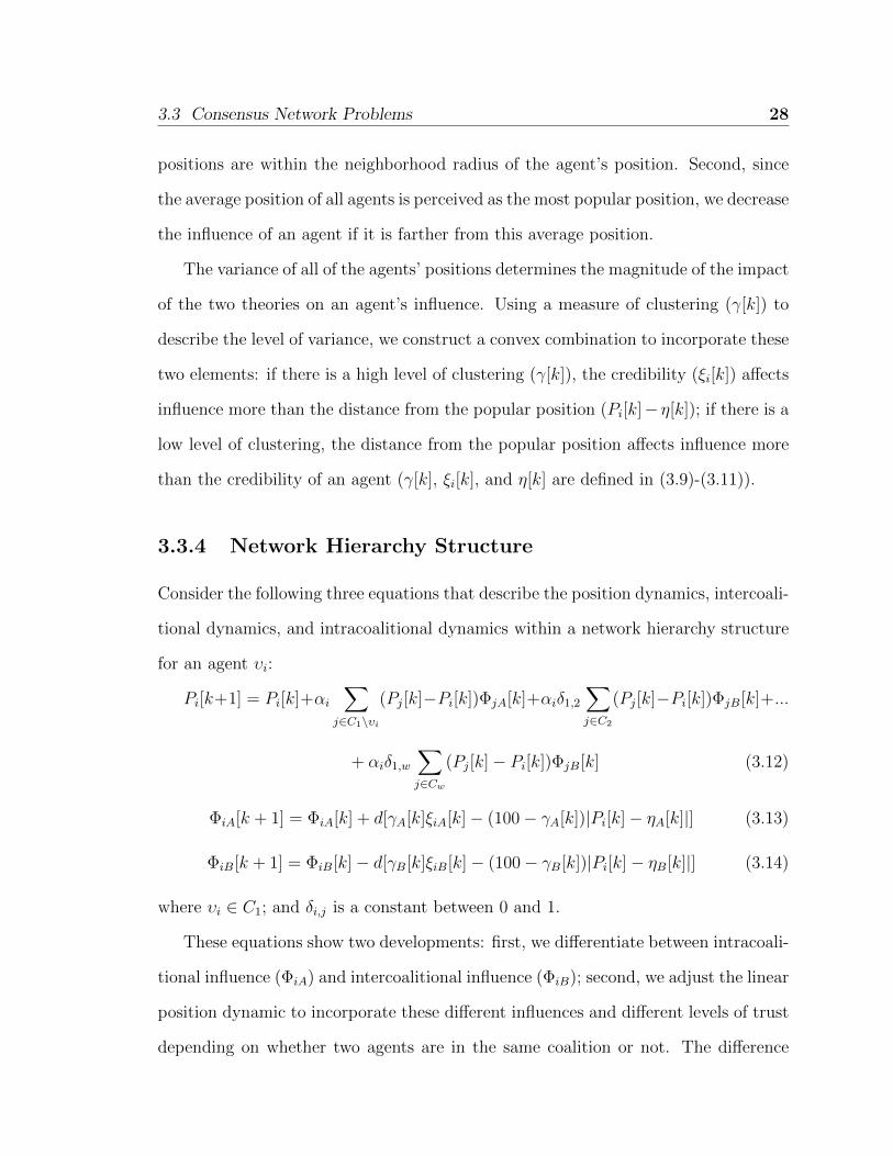
3.3.4 Network Hierarchy Structure
Consider the following three equations that describe the position dynamics, intercoali-
tional dynamics, and intracoalitional dynamics within a network hierarchy structure
for an agent υi:
Pi[k+1] = Pi[k]+αi∑
j∈C1\υi
(Pj[k]−Pi[k])ΦjA[k]+αiδ1,2
∑j∈C2
(Pj[k]−Pi[k])ΦjB[k]+...
+ αiδ1,w
∑j∈Cw
(Pj[k]− Pi[k])ΦjB[k] (3.12)
ΦiA[k + 1] = ΦiA[k] + d[γA[k]ξiA[k]− (100− γA[k])|Pi[k]− ηA[k]|] (3.13)
ΦiB[k + 1] = ΦiB[k]− d[γB[k]ξiB[k]− (100− γB[k])|Pi[k]− ηB[k]|] (3.14)
where υi ∈ C1; and δi,j is a constant between 0 and 1.
These equations show two developments: first, we differentiate between intracoali-
tional influence (ΦiA) and intercoalitional influence (ΦiB); second, we adjust the linear
position dynamic to incorporate these different influences and different levels of trust
depending on whether two agents are in the same coalition or not. The difference
3.3 Consensus Network Problems 29
between intracoalitional influence and intercoalitional influence is that the first satu-
rates to 100 as time progresses while the second decreases to 0 as time progresses. At
the beginning of the simulation, each agent’s intercoalitional influence value is equal
to its intracoalitional influence value (ΦA[0] = ΦB[0]). This reflects the assumption
that while at the beginning of a negotiation, agents are influenced by anyone, as time
progresses, they pay more attention to those within their own coalition. Thus, agents
within a coalition can have different influences on each other than agents in different
coalitions.
The δi,j’s represent how much one coalition affects another (the trust between
coalitions or the amount of interactions one coalition has with the other). Thus,
while each agent broadcasts two different influences (one for agents within its coalition
and one for agents outside of its coalition), the δi,j’s allow for different coalitions to
pay different levels of attention to the same intercoalitional influence broadcast. It
essentially creates two consensus systems: one within coalitions and one between
coalitions.
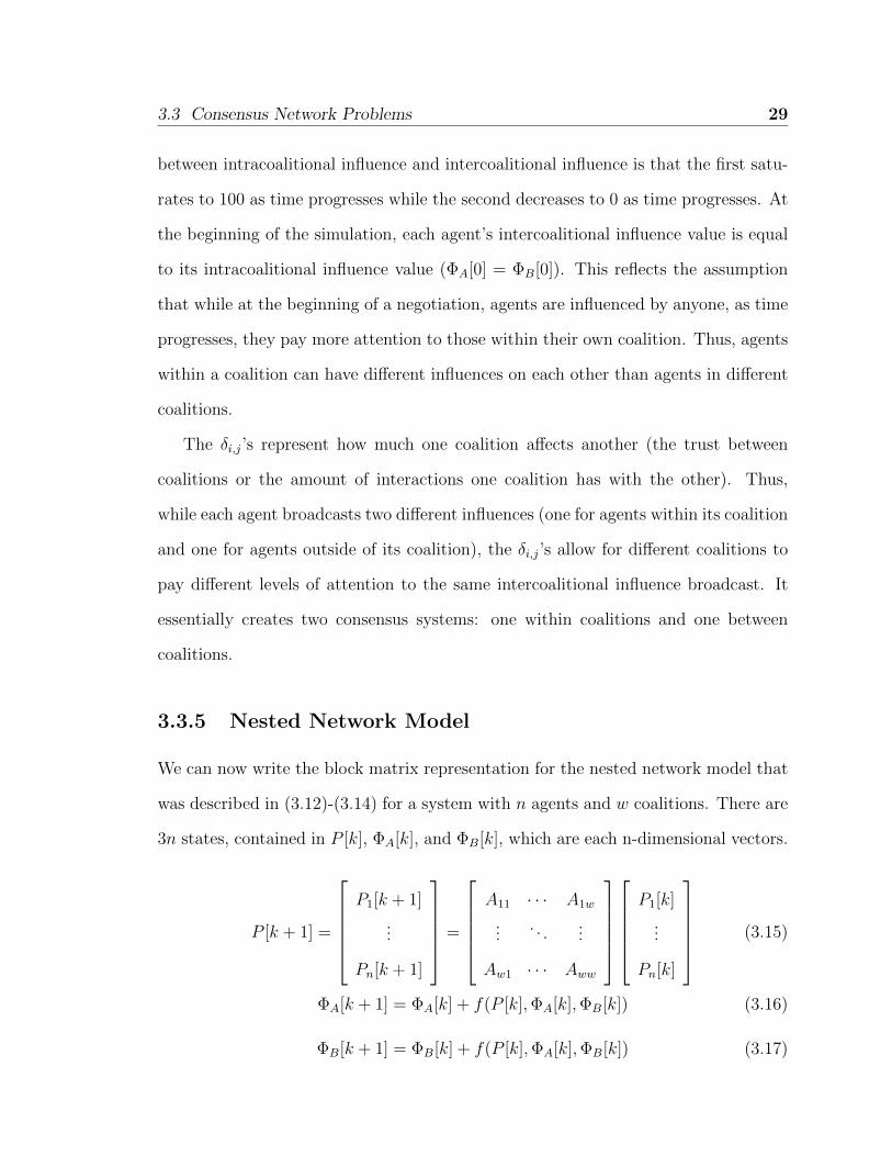
3.3.5 Nested Network Model
We can now write the block matrix representation for the nested network model that
was described in (3.12)-(3.14) for a system with n agents and w coalitions. There are
3n states, contained in P [k], ΦA[k], and ΦB[k], which are each n-dimensional vectors.
P [k + 1] =
P1[k + 1]
...
Pn[k + 1]
=
A11 · · · A1w
.... . .
...
Aw1 · · · Aww
P1[k]
...
Pn[k]
(3.15)
ΦA[k + 1] = ΦA[k] + f(P [k],ΦA[k],ΦB[k]) (3.16)
ΦB[k + 1] = ΦB[k] + f(P [k],ΦA[k],ΦB[k]) (3.17)
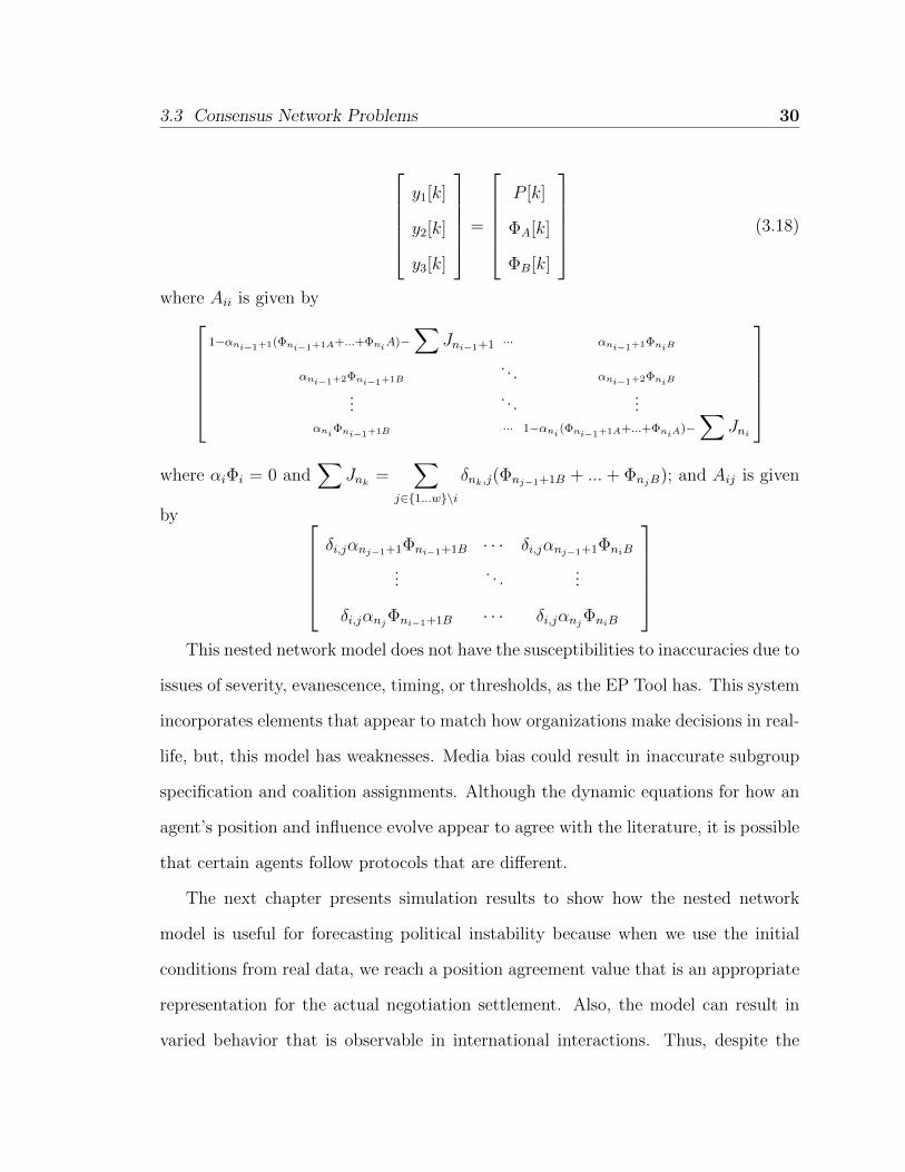
3.3 Consensus Network Problems 30
y1[k]
y2[k]
y3[k]
=
P [k]
ΦA[k]
ΦB[k]
(3.18)
where Aii is given by1−αni−1+1(Φni−1+1A+...+ΦniA)−
∑Jni−1+1 ··· αni−1+1ΦniB
αni−1+2Φni−1+1B
... αni−1+2ΦniB
......
...αniΦni−1+1B ··· 1−αni (Φni−1+1A+...+ΦniA
)−∑
Jni
where αiΦi = 0 and
∑Jnk
=∑
j∈{1...w}\i
δnk,j(Φnj−1+1B + ... + ΦnjB); and Aij is given
by δi,jαnj−1+1Φni−1+1B · · · δi,jαnj−1+1ΦniB
.... . .
...
δi,jαnjΦni−1+1B · · · δi,jαnj
ΦniB
This nested network model does not have the susceptibilities to inaccuracies due to
issues of severity, evanescence, timing, or thresholds, as the EP Tool has. This system
incorporates elements that appear to match how organizations make decisions in real-
life, but, this model has weaknesses. Media bias could result in inaccurate subgroup
specification and coalition assignments. Although the dynamic equations for how an
agent’s position and influence evolve appear to agree with the literature, it is possible
that certain agents follow protocols that are different.
The next chapter presents simulation results to show how the nested network
model is useful for forecasting political instability because when we use the initial
conditions from real data, we reach a position agreement value that is an appropriate
representation for the actual negotiation settlement. Also, the model can result in
varied behavior that is observable in international interactions. Thus, despite the
3.3 Consensus Network Problems 31
weaknesses of the nested network model, we hypothesize that it is a step in discovering
the “Newton’s Laws” that explain the social dynamics that create political instability.
Chapter 4
Consensus Simulation
This chapter is composed of three section that focus on the simulation results of
the nested network model presented in (3.15) - (3.18). The first section describes
some of the general behavior of the nested network model that is apparent from the
simulation graphs. The second section discusses three simulation results that can
indicate political instability. The third section applies the nested network model
to initial conditions from the Israeli-Palestinian Conflict in 1987 and compares the
simulated results with the negotiated agreement from Oslo in 1993 and political events
in between.
4.1 Model Behavior
Graphs displaying the evolving positions of the agents are used for verification against
values in the literature and in real-life. An issue is chosen with a defined spectrum
between two extremes, represented by the real numbers between 0 and 100. An agent
is assigned a position value between 0 and 100 that accurately represents the agent’s
belief about the issue. Similarly, values between 0 and 100 are determined for each
32
4.1 Model Behavior 33
agent’s influence, salience, and firmness.
The visualization of the simulation displays only the positions of each agent as
time progresses. Agents’ positions are graphed on the vertical axis, with each line’s in-
tercept located at the initial value. Time is on the horizontal axis – a series of integers
following the number of rounds. While such a discrete system does not represent the
real-life continuous changing of salience, influence, firmness, and position, the exact
values for these four variables only matter when the agents meet. By modeling the
meetings of the agents, which may occur at regular or irregular intervals, this model
is in agreement with the theoretical structure of international conflict negotiations.
An example of the simulation results of the nested network model (3.15) - (3.18)
are presented in Figure 4.1. With 11 agents in total, the first six agents are in one
coalition and the last five are in another. The initial conditions of this simulation are
as follows:
P [0] = {85, 85, 70, 70, 60, 30, 25, 20, 20, 0, 0},ΦA[0] = ΦB[0] = {85, 85, 60, 100, 100, 60,
100, 70, 100, 20, 10}, S[0] = {85, 90, 50, 99, 80, 75, 95, 85, 95, 95, 80}, F [0] = {97, 97, 96,
98, 98, 96, 98, 97, 99, 96, 95}, ε = 10, d = .002, a = .000001, and δ1 = δ2 = .8.
The graph shows 11 lines, each showing how the positions of one of the 11 agents
changes over time. It is evident from the slopes of the lines how quickly agents change
positions. Once all agents have stopped moving, the simulation ends. While in this
simulation, δi,j = δj,i, if they were not equal, the position agreement value would be
attracted more to the extreme position of the coalition that pays the least attention
to the other coalition.
It is unreasonable to assume that all of the coalitions eventually completely agree
on an issue; however, they can get close enough that if a resolution was proposed
between them that the coalitions would agree. If the position agreement values for
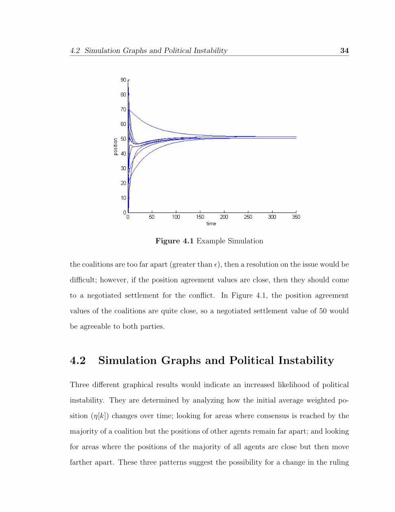
4.2 Simulation Graphs and Political Instability 34
Figure 4.1 Example Simulation
the coalitions are too far apart (greater than ε), then a resolution on the issue would be
difficult; however, if the position agreement values are close, then they should come
to a negotiated settlement for the conflict. In Figure 4.1, the position agreement
values of the coalitions are quite close, so a negotiated settlement value of 50 would
be agreeable to both parties.
4.2 Simulation Graphs and Political Instability
Three different graphical results would indicate an increased likelihood of political
instability. They are determined by analyzing how the initial average weighted po-
sition (η[k]) changes over time; looking for areas where consensus is reached by the
majority of a coalition but the positions of other agents remain far apart; and looking
for areas where the positions of the majority of all agents are close but then move
farther apart. These three patterns suggest the possibility for a change in the ruling
4.2 Simulation Graphs and Political Instability 35
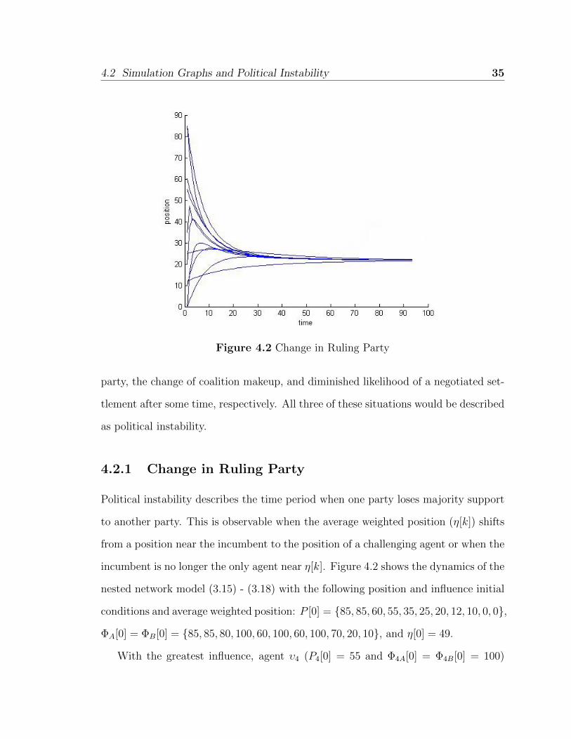
Figure 4.2 Change in Ruling Party
party, the change of coalition makeup, and diminished likelihood of a negotiated set-
tlement after some time, respectively. All three of these situations would be described
as political instability.
4.2.1 Change in Ruling Party
Political instability describes the time period when one party loses majority support
to another party. This is observable when the average weighted position (η[k]) shifts
from a position near the incumbent to the position of a challenging agent or when the
incumbent is no longer the only agent near η[k]. Figure 4.2 shows the dynamics of the
nested network model (3.15) - (3.18) with the following position and influence initial
conditions and average weighted position: P [0] = {85, 85, 60, 55, 35, 25, 20, 12, 10, 0, 0},
ΦA[0] = ΦB[0] = {85, 85, 80, 100, 60, 100, 60, 100, 70, 20, 10}, and η[0] = 49.
With the greatest influence, agent υ4 (P4[0] = 55 and Φ4A[0] = Φ4B[0] = 100)
4.2 Simulation Graphs and Political Instability 36
could be the incumbent party, leading the coalition of agents {υ1, υ2, υ3, υ4, υ5, υ7}.
Although the average weighted position remains around 50 for the first five rounds, as
time progresses, η[k] decreases, eventually reaching values in the 30’s and 20’s. This
represents a change in the majority of opinion on the issue. While it is possible that
the incumbent party could project a change in position and remain in power, it is no
longer the only agent whose position is near to the average weighted position. Also,
the intracoalitional influences of all of the agents increases over time and eventually
saturates at 100. Therefore, the initial advantages of being highly influential and
at the most powerful position are lost. It is likely that another party could try to
take power. Such a political change would definitely be characterized as political
instability.
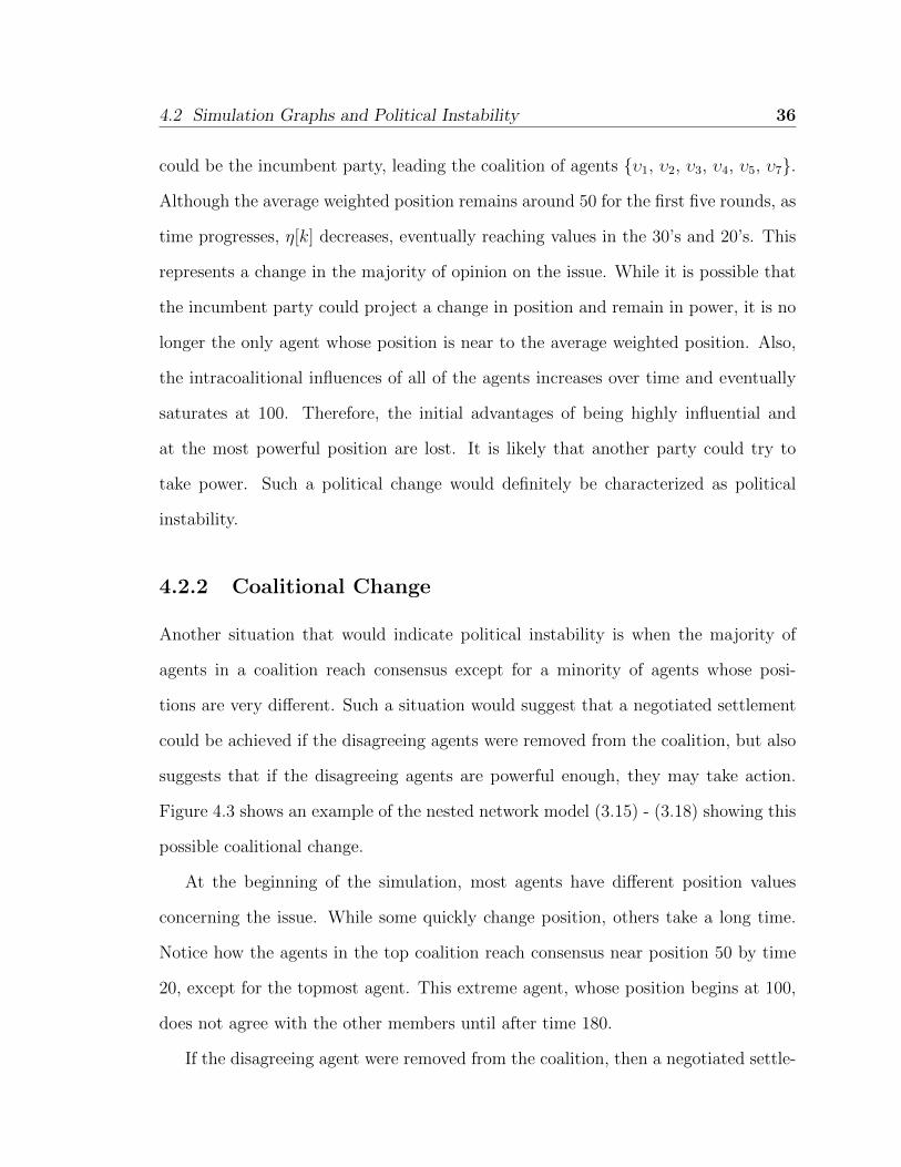
4.2.2 Coalitional Change
Another situation that would indicate political instability is when the majority of
agents in a coalition reach consensus except for a minority of agents whose posi-
tions are very different. Such a situation would suggest that a negotiated settlement
could be achieved if the disagreeing agents were removed from the coalition, but also
suggests that if the disagreeing agents are powerful enough, they may take action.
Figure 4.3 shows an example of the nested network model (3.15) - (3.18) showing this
possible coalitional change.
At the beginning of the simulation, most agents have different position values
concerning the issue. While some quickly change position, others take a long time.
Notice how the agents in the top coalition reach consensus near position 50 by time
20, except for the topmost agent. This extreme agent, whose position begins at 100,
does not agree with the other members until after time 180.
If the disagreeing agent were removed from the coalition, then a negotiated settle-
4.2 Simulation Graphs and Political Instability 37
Figure 4.3 Coalitional Change
ment could occur sooner. If an agreement between coalition was more important to
a coalition’s agents than having every agent agree, then they may choose to remove
the disagreeing agents from their coalition in order to prevent a longer conflict. This
change can occur as long as the disagreeing agent does not have some sort of veto-
power or other crucial attribute. It is quite reasonable to assume that a number of
agents could believe that placating outside enemies is more important than placating
interior extremist groups.
If the disagreeing agents are the most powerful agents, it is also possible that they
will not be pleased with the rest of the coalition agreeing at a position value so far
from its own. Having a few agents so far from the rest of the agents in a coalition
could result in political contention, a coup by the disagreeing agents, or some other
change in government power – all examples of political instability.
4.2 Simulation Graphs and Political Instability 38
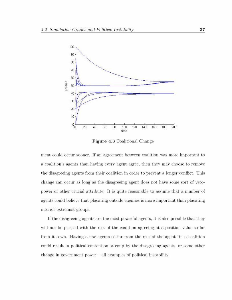
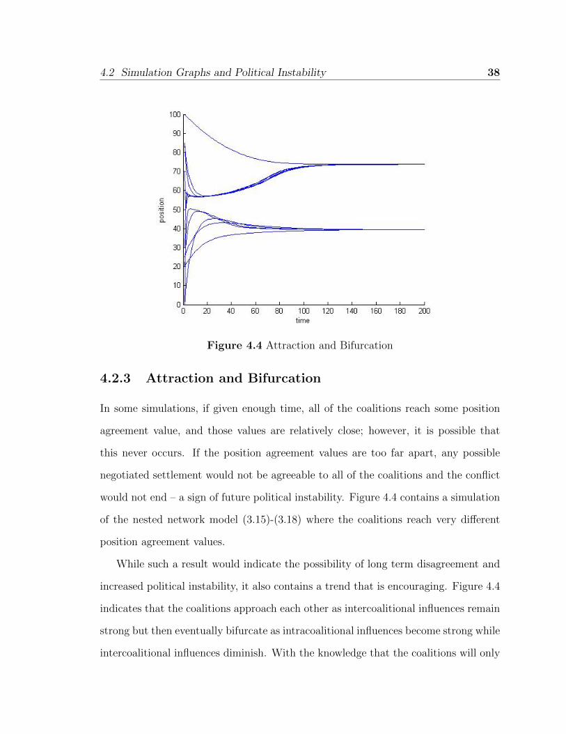
Figure 4.4 Attraction and Bifurcation
4.2.3 Attraction and Bifurcation
In some simulations, if given enough time, all of the coalitions reach some position
agreement value, and those values are relatively close; however, it is possible that
this never occurs. If the position agreement values are too far apart, any possible
negotiated settlement would not be agreeable to all of the coalitions and the conflict
would not end – a sign of future political instability. Figure 4.4 contains a simulation
of the nested network model (3.15)-(3.18) where the coalitions reach very different
position agreement values.
While such a result would indicate the possibility of long term disagreement and
increased political instability, it also contains a trend that is encouraging. Figure 4.4
indicates that the coalitions approach each other as intercoalitional influences remain
strong but then eventually bifurcate as intracoalitional influences become strong while
intercoalitional influences diminish. With the knowledge that the coalitions will only
4.3 Case Study: Israeli-Palestinian Conflict 39
drift farther away, if a negotiated settlement had been proposed early, then it is pos-
sible that they could have reached an agreement instead of waiting for full consensus
within the coalitions.
In Figure 4.4, if a negotiated position had been suggested around value 52 between
time periods 20-40, a majority of the agents would have been within ε – close enough
to support the settlement decision. After this time, the coalitions drift farther apart.
Eventually, the distance between their position agreement values becomes so large,
that any proposed negotiated settlement value for the issue would not be agreeable
to both parties. Aware of the impending division, policymakers could try to influence
coalitions to agree to a settlement earlier in order to prevent the bifurcation and
resulting long-term political instability from occurring.
4.3 Case Study: Israeli-Palestinian Conflict
This section describes an application of the nested network model (3.15) - (3.18)
to the Israeli-Palestinian conflict. The purpose is to verify the model by analyzing
the simulation results against the literature and real-life results. This is done by
comparing the changes in positions of the agents and the final position agreement
value of the coalitions. The simulation is analyzed for any of the three graphical
results that indicate political instability, as explained in Section 4.2.
4.3.1 Motivation
The Israeli-Palestinian Conflict has many characteristics that make it a good case
study. There exists a great deal of publicly available data. There have been prior
attempts to model this conflict which are available for review and analysis, such as [24]
and [5]. Two coalitions are well-defined and have integrity over the time window of
4.3 Case Study: Israeli-Palestinian Conflict 40
interest. The conflict spans decades with frequent events. Despite these advantages,
there are certain challenges involved in modeling the Israeli-Palestinian Conflict.
4.3.2 Unique Challenges
There are certain characteristics about the Israeli-Palestinian Conflict that are unique
and make any modeling attempt difficult. Because the Holy Land contains popula-
tions and holy sites of Judaism, Christianity, and Islam, international conflicts are
susceptible to strong, emotional opinions and events. The Israeli-Palestinian Conflict
does not fit the conventional description of warfare, which is an outdated definition
of action and response. [44] suggests that Israel, as a more western-style democracy,
has weaknesses of dealing with borders, headquarters and conventional forces. Is-
raeli dominance and Palestinian weakness in the conventional military arena encour-
ages Palestinians to use asymmetric means to attack Israelis forces [32]. Therefore,
a forecasting model should incorporate unconventional interactions, such as suicide
bombing, a commonly-used tool since 1993.
While we apply the nested network model to the question of Palestinian nation-
hood, it is only one of many issues in the conflict (i.e. control over allotted lands, holy
places, arable land, freedom of access, water resources, settlements, security, economic
freedom, precise border demarcations, geopolitical strategy, quid pro quo, Jerusalem,
legal status of Palestinian refugees, the Golan Heights, international recognition, and
resource distribution). These other volatile issues are important, and it is likely that
whenever peace accords occur, there will be consolidation and balance between them.
By focusing on only one issue, we ignore the conflict’s mixed nature, but create a
tractable area of analysis.
4.3 Case Study: Israeli-Palestinian Conflict 41
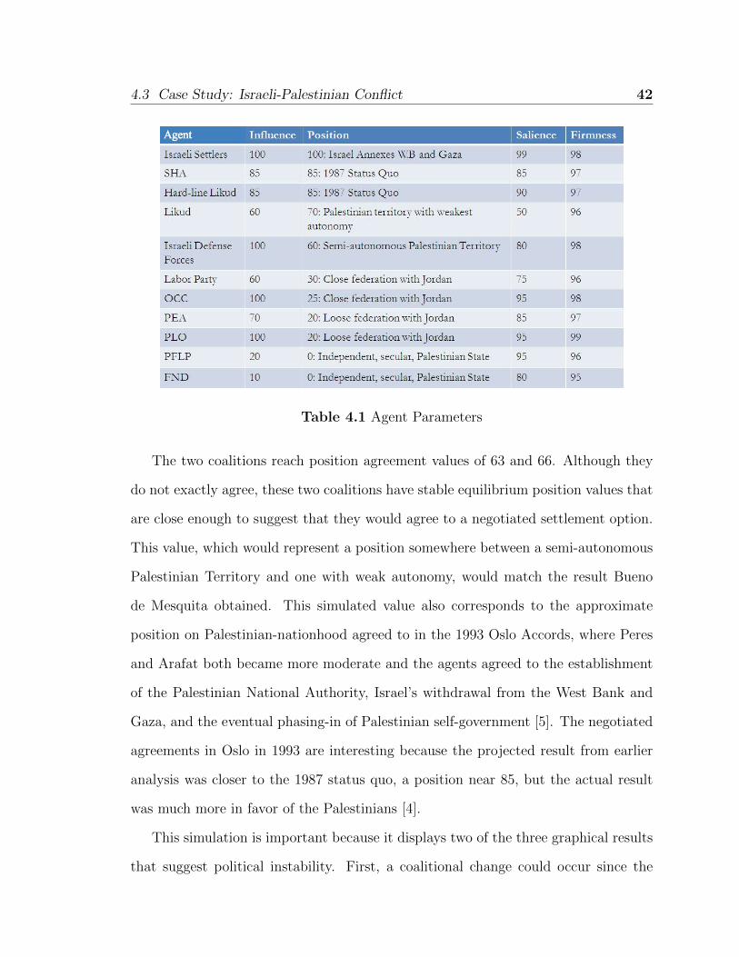
4.3.3 Agent Subgroups
The simulation below is focused on the period from 1987 until the Oslo Accords in
1993. The subgroup agents are the Israeli Settlers, SHA, Hard-line Likud, Likud,
Israeli Defense Forces, Labor Party, OCC, PEA, PLO, PFLP, and FND. These were
determined by [5]. These agents are organized into two major coalitions: Israeli
(Israeli Settlers, SHA, Hard-line Likud, Likud, Israeli Defense Forces, and Labor
Party) and Palestinian (OCC, PEA, PLO, PFLP, and FND).
4.3.4 Parameter Table
Table 4.1 contains parameter value estimates for the agent subgroups for 1987. The
close federation with Jordan represents a non-autonomous political entity that would
be federated with Jordan. The parameter values for position, salience, and influence
were obtained through Bueno de Mesquita’ collaboration with Shmuel Eisenstadt and
Harold Saunders as reported in [5]. We determined the firmness values by researching
the profiles of each agent subgroup.
4.3.5 Model Verification
Figure 4.5 shows how the position values of the 11 agents evolve according to the
dynamics presented in (3.15) - (3.18), with the first six agents in one coalition, the
last five agents in another, and the following initial conditions:
P [0] = {100, 85, 85, 70, 60, 30, 25, 20, 20, 0, 0},ΦA[0] = ΦB = {100, 85, 85, 60, 100, 60,
100, 70, 100, 20, 10}, S[0] = {99, 85, 90, 50, 80, 75, 95, 85, 95, 95, 80}, F [0] = {98, 97, 97,
96, 98, 96, 98, 97, 99, 96, 95}, ε = 10, δ1 = δ2 = .8, d = .0002, and a = .00001.
4.3 Case Study: Israeli-Palestinian Conflict 42
Table 4.1 Agent Parameters
The two coalitions reach position agreement values of 63 and 66. Although they
do not exactly agree, these two coalitions have stable equilibrium position values that
are close enough to suggest that they would agree to a negotiated settlement option.
This value, which would represent a position somewhere between a semi-autonomous
Palestinian Territory and one with weak autonomy, would match the result Bueno
de Mesquita obtained. This simulated value also corresponds to the approximate
position on Palestinian-nationhood agreed to in the 1993 Oslo Accords, where Peres
and Arafat both became more moderate and the agents agreed to the establishment
of the Palestinian National Authority, Israel’s withdrawal from the West Bank and
Gaza, and the eventual phasing-in of Palestinian self-government [5]. The negotiated
agreements in Oslo in 1993 are interesting because the projected result from earlier
analysis was closer to the 1987 status quo, a position near 85, but the actual result
was much more in favor of the Palestinians [4].
This simulation is important because it displays two of the three graphical results
that suggest political instability. First, a coalitional change could occur since the
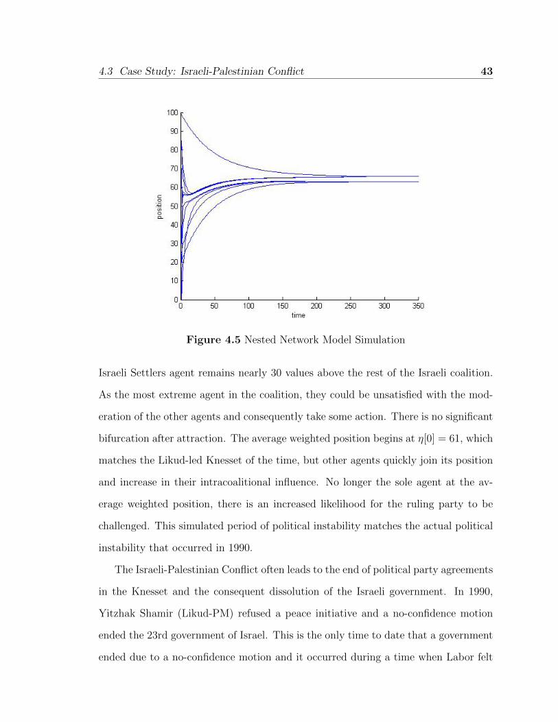
4.3 Case Study: Israeli-Palestinian Conflict 43
Figure 4.5 Nested Network Model Simulation
Israeli Settlers agent remains nearly 30 values above the rest of the Israeli coalition.
As the most extreme agent in the coalition, they could be unsatisfied with the mod-
eration of the other agents and consequently take some action. There is no significant
bifurcation after attraction. The average weighted position begins at η[0] = 61, which
matches the Likud-led Knesset of the time, but other agents quickly join its position
and increase in their intracoalitional influence. No longer the sole agent at the av-
erage weighted position, there is an increased likelihood for the ruling party to be
challenged. This simulated period of political instability matches the actual political
instability that occurred in 1990.
The Israeli-Palestinian Conflict often leads to the end of political party agreements
in the Knesset and the consequent dissolution of the Israeli government. In 1990,
Yitzhak Shamir (Likud-PM) refused a peace initiative and a no-confidence motion
ended the 23rd government of Israel. This is the only time to date that a government
ended due to a no-confidence motion and it occurred during a time when Labor felt
4.3 Case Study: Israeli-Palestinian Conflict 44
especially emboldened. Consequently, Peres (Alignment/Labor) was asked to try to
form a government, and almost did so with Israeli Settler support, but eventually
failed. The above simulation is interesting because it shows two things: a quick slide
of Israeli agents from the upper extreme to the middle ground and the consequent
loss of Likud having majority control over the average weighted position; and how
the Israel Settlers were much more extreme than the rest of the Israeli agents and
would have been dissatisfied with their moderate positions.
The Israeli agents’ moderation and the Israeli Settler’s continued extremism on the
issue of Palestinian statehood would have been apparent had our model been applied
in 1987. The simulation result would have been a forecast of political instability,
which turned out to be the case with the no-confidence vote and attempt to form a
new government described above.
Chapter 5
Conclusions
The model described in (3.15) - (3.18) appears to be useful for forecasting political
instability because the simulated position agreement value matched the real-life value
and because the simulation dynamics matched the lack of support for the Likud-led
Knesset in 1990. We have explored an external data analysis method and found cer-
tain susceptibilities to error that directed us to focus on internal dynamics models.
With the assumption that people change their positions on issues based on the assim-
ilation of those around them, we used consensus model elements as our foundation.
Finding our linear position dynamics (3.5) to be limited in their ability to simulate
stable disagreement, we added nonlinear influence dynamics (Section 3.3.3) and a
network hierarchical structure (Section 3.3.4) – thus allowing for different intracoali-
tional and intercoalitional influences as well as different levels of attention or trust
between coalitions. Our findings suggest that an internal dynamics model (3.15) -
(3.18) built from consensus model elements may be capable of forecasting political
instability. We believe that although our nested coupled system is not the complete
“Newton’s Law” that needs to be understood in order to perfectly forecast political
instability; nevertheless, the results are encouraging enough to suggest that consensus
45
5.1 Further Work 46
models are an appropriate tool for the problem.
5.1 Further Work
While this paper has summarized the two major modeling methodologies and pre-
sented our own variation of one of them, there are additional research ideas that can
be explored. With region-specific adaptations, our model could be applied to other
conflicts. Another variation would involve pairwise influence. Although this concept
is partially addressed by using multiple δ’s in (3.9), it could be done by creating a
separate influence for each agent pair in the model. Adding dynamics for the salience
and firmness of agents would be another interesting variation for our model.
Dual-state agents, where each agent has a true state and a declared state, would
better reflect the real-life negotiation situation of the Israeli-Palestinian Conflict. It
is likely that the declared position of an agent would be more aggressive, while its
true position would be less so. In the West, this hidden position may be permanently
obscured; however, in the Middle East, the true position could be revealed given
enough time and a sufficient amount of leaked information.
A weighted arrangement where as each round proceeds, each agent places more
weight on the true position and less weight on the declared position, could be con-
structed. By varying the weights and the number of rounds necessary until full
disclosure, different simulations could be done.
An unresolved issue is whether influence is a zero-sum commodity. This depends
on if an agent’s influence is described as the share of influence or if an agent can
increase in influence without another agent losing influence. In certain applications,
it makes sense for influence to be some finite quantity that is shared; in others, it
makes sense for an agent to be able to increase or decrease in influence without
5.1 Further Work 47
affecting other agents’ influence. In this paper, we did not treat influence as a zero-
sum commodity, but it would be interesting to see how such a change would affect
the dynamics of the simulation.
We view this thesis as an attempt to summarize the two approaches to forecasting
political instability and to present innovations on previous attempts. Encouraged
by the results predicting the political instability in the Knesset in 1990, we plan on
continuing to investigate this research area in future work.
Bibliography
[1] Acemoglu, D., A. Ozdaglar, and A. ParandehGheibi Spread of Misinformation in
Social Networks. LIDS Report 2812, 2009.
[2] Andriole, S., and G. Hopple Defense Applications of Artificial Intelligence. Lex-
ington, MA: Lexington, 1988.
[3] Axelrod, R. The Complexity of Cooperation: Agent-Based Models of Competition
and Collaboration. Princeton, NJ: Princeton University Press, 1997.
[4] Bueno de Mesquita, B. Multilateral Negotiations: A Spatial Analysis of the Arab-
Israeli Dispute. International Organization, 44(3):317-340, 1990.
[5] Bueno de Mesquita, B. The Predictioneer’s Game. New York: Random House,
2009.
[6] Bueno de Mesquita, B., A. Smith, R. Siverson, and J. Morrow The Logic of
Political Survival. Cambridge, Mass: The MIT Press, 2003.
[7] Carbonell, J. POLITICS: Automated Ideological Reasoning. Cognitive Science,
2:27-51, 1978.
[8] Charness, G. and M. Jackson Group Play in Games and the Role of Consent in
Network Formation. Journal of Economic Theory 136(1):417-445, 2007.
48
BIBLIOGRAPHY 49
[9] Chatterjee, K., B. Dutta, D. Ray, and S. Sengupta A Noncooperative Theory of
Coalitional Bargaining. Review of Economic Studies 60(1):463-477, 1993.
[10] Chatterjee, S. and E. Senata Towards Consensus: Some Convergence Theorems
on Repeated Averaging. Journal of Applied Probability: 14:159-164, 1977.
[11] DeGroot, M. Reaching a Consensus. Journal of the American Statistical Associ-
ation 69:118-121, 1974.
[12] DeMarzo, P., D. Vayanos, and J. Zwiebel Persuasion Bias, Social Influence and
Unidimensional Opinions. Quarterly Journal of Economics 118:909-968, 2003.
[13] Friedkin, N., and E. Johnsen Social Influence and Opinions. Journal of Mathe-
matical Sociology 15:193-206, 1990.
[14] Friedkin, N., and E. Johnsen Social Positions in Influence Networks. Social Net-
works 19:209-222, 1997.
[15] Galeotti, A., and C. Ghiglino, and F. Squintani Strategic Information Transmis-
sion in Networks. Preprint, 2009.
[16] Geoffrey, M. Media Bias, Right Topic Overview. In R. Carlisle, Encyclopedia of
Politics: The Left and the Right Thousand Oaks, CA: Sage Reference, 758-760,
2005.
[17] Gladwell, M. Blink. New York City: Little, Brown, and Company, 105, 2005.
[18] Gray, C. On Strategic Performance. Joint Force Quarterly, 30-36, 1995-6.
[19] Hannan, Michael Operational Net Assessment: A Framework for Social Network
Analysis and Requirements for Critical Debate. Naval War College Newport RI
Joint Military Operations Department, A265464, 2005.
BIBLIOGRAPHY 50
[20] Hegselmann, R., and U. Krause Opinion Dynamics and Bounded Confidence
Models, Analysis, and Simulations. Journal of Artificial Societies and Social Sim-
ulation 5(3):1-33, 2002.
[21] Herman, E., and N. Chomsky Manufacturing Consent: The Political Economy
of the Mass Media. New York: Pantheon Books, 1988.
[22] Hudson, V. ed. Artificial Intelligence and International Politics. Portland, OR:
Book News, 1991.
[23] Hudson, V., and P. Schrody, and R. Whitmer A New Kind of Social Science:
Moving Ahead with Reverse Wolfram Models Applied to Event Data. Honolulu,
HI: Annual Meeting of the International Studies Association, 2005.
[24] Hudson, V., P. Schrody, and R. Whitmer Discrete Sequence Rule Models as
a Social Science Methodology: An Exploratory Analysis of Foreign Policy Rule
Enactment Within Palestinian-Israeli Event Data. Foreign Policy Analysis, 105-
126, 2008.
[25] Jackson, M. Social and Economic Networks. Princeton, NJ: Princeton University
Press, 2008.
[26] Krause, U. A Discrete Nonlinear and Nonautonomous Model of Consensus For-
mation. in Communications in Difference Equations, S. Elaydi, G. Ladas, J.
Popenda, and J. Rakowski, eds., Amsterdam: Gordon and Breach, 2000.
[27] Lopez-Pintado, D., Diffusion in Complex Social Networks. Games and Economic
Behavior 62(2):573-590, 2008.
BIBLIOGRAPHY 51
[28] Lopez-Pintado, D., and D. Watts Social Influence, Binary Decisions and Collec-
tive Dynamics. New York, Department of Sociology, Columbia University, mimeo,
2006.
[29] Lorenz, J. A Stabilization Theorem for Dynamics of Continuous Opinions. Phys-
ica A 355:217-223, 2005.
[30] Majeski, S. A Recommendation Model of War Initiation: The Plausability and
Generalizability of General Cultural Rules. In Artificial Intelligence and National
Security, ed. Cimbala, S., Lexington, MA: Lexington Books, 1987.
[31] Mefford, D. Steps Toward Artificial Intelligence: Rule-Based, Case-Based and
Explanation-Based Models of Politics. In Artificial Intelligence and International
Politics ed. V. Hudson, Boulder: Westview, 1991.
[32] Metz S., and D. Johnson Asymmetry and U.S. Military Strategy: Definition,
Background, and Strategic Concepts. Carlisle: Strategic Studies Institute, 2001.
[33] Moreno, Y., R. Pastor-Satorras, and A. Vespignani Epidemic Outbreaks in Com-
plex Heterogeneous Networks. European Physics Journal B 26:521-529, 2002.
[34] Myerson, R. Game Theory: Analysis of Conflict. Cambridge, Mass.: Harvard
University Press, 1977.
[35] Newman, M.The Spread of Epidemic Disease on Networks. Physical Review E
66:061628, 2002.
[36] Olfati-Saber, R., and R. Murray Consensus Problems in Networks of Agents with
Switching Topology and Time-delays. IEEE Transactions on Automatic Control
49, no. 9:1520-1533, 2004.
[37] Patai, R.The Arab Mind. New York: Scribner, 1973.
BIBLIOGRAPHY 52
[38] Ray, J. and B. Russett The Future as Arbiter of Theoretical Controversies: Pre-
dictions, Explanations, and the End of the Cold War. British Journal of Political
Science, 441-470, 1996.
[39] Robinson, C. Perron Frobenius Theorem. Northwestern University.
http://www.math.northwestern.edu/ clark/354/2002/perron.pdf, 2002.
[40] Roskin, M., and J. Coyle Politics of the Middle East. Upper Sadle River, NJ:
Pearson Education, 2004.
[41] Slikker, M., and A. van den Nouweland Social and Economics Networks in Co-
operative Game Theory. Amsterdam: Kluwer, 2001.
[42] Sylvan, D., A. Goel and B. Chandrasekran Analyzing Political Decision Mak-
ing from an Information Processing Perspective: JESSE. American Journal of
Political Science, 34:74-123, 1990.
[43] Thompson, C. Can Game Theory Predict When Iran Will Get the Bomb?. The
New York Times, MM20, 2009.
[44] Thornton, R. Asymmetric Warfare. Malden, MA: Polity Press, 2007.
[45] Thorson, S. and D. Sylvan Counterfactuals and the Cuban Missile Crisis. Inter-
national Studies Quarterly, 26:537-71, 1982.
[46] Tsitsiklis, J., D. Bertsekas, and M. Athans Distributed Asynchronous Deter-
ministic and Stochastic Gradient Optimization Algorithms. IEEE Transactions on
Automatic Control 31, no. 9, 803-812, 1986.
[47] Wasserman, S., and K. Faust Social Network Analysis: Methods and Applica-
tions. Cambridge: Cambridge University Press, 1994.
BIBLIOGRAPHY 53
[48] Wielhouwer, P. Toward Information Superiority: The Contribution of Opera-
tional Net Assessment. Air and Space Power Journal, Fall, 2005.
[49] Wright, R. Dreams and Shadows: The Future of the Middle East. New York City:
Penguin Press, 2008.
[50] Young, H.P. The Diffusion of Innovations on Social Networks. The Economy as a
Complex Evolving System, Vol. 3, L. Blume and S. Durlauf, eds., Oxford: Oxford
University Press, 2003.