Forecasting Financial Statements with No plugs and No Circularity ...

Forecasting Financial Statements with No plugs and No Circularity

Ignacio Vélez–Pareja Universidad Tecnológica de Bolívar

Cartagena, Colombia [email protected]

[email protected]

First Version: July 20, 2007 This version: May 28, 2009

ii

Abstract

Typical textbooks on corporate finance and forecasting and budgeting recommend “closing” and matching the financial statements using what is known as a plug. A plug is a formula to match the Balance Sheet using differences in some items listed in it in such a way that the accounting equation holds. This is a very easy way to do it but it encompasses some risks. The risks are that certain numbers in the financial statements could be in error and still the plug would indicate that everything is correct because the Balance Sheet matches.

In this work we show how to construct financial statement without plugs and circularity.

The basic learning objective of this work is to develop the students’ and practitioners’ abilities to find information inside and outside the firm for constructing a proper financial model to forecast financial statements without plugs and without circularity.

We explain how the plug works and which its drawbacks are. We present a detailed example that can be used by any student, teacher or practitioner to properly construct consistent financial statements. The example shows how to relate different cells in the spreadsheet and the reader is encouraged to develop the example by herself.

We present some criticisms received against the no plug, no circularity approach and we discuss them. Finally, as a conclusion we suggest that the use of plugs should be discontinued when teaching forecasting financial statements and budgeting.

JEL Classification:

E47, G31

Keywords Accounting, Forecasting Financial Statements, Decision Making, plugs, Planning

and control, double entry principle, unbalancing problem.

To plug or not to plug, that is the question. No plugs, No Circularity: A Better Way to Forecast Financial Statements

1

Introduction

Why is necessary to work with forecasted financial statements? Forecasting

financial statements is not optional for the management because it can provide a guide to

the future performance of the firm. Doing prospective analysis for the long term is of

utmost importance in order to develop strategies for meeting the challenges that will arise

in the future. For most firms (non traded firms), it is vital to have a financial model that

allows management to control value creation. Constructing cash flows from the financial

statements and having a permanent assessment of the firm value allow management to

implement management based on value.

A consistent financial model is useful to examine in advance and anticipate the

economic effect of a decision. To do this we can use sensitivity analysis, scenario analysis

and simulation (Monte Carlo Simulation, MCS).

Financial models are multipurpose tools and can be used for other purposes as well:

1. When we plan to raise funds for a new firm or a new project in an ongoing

concern.

2. When we need to set its value for selling or merging purposes.

3. When we apply for bond issues or private financing.

Many centuries ago Luca Pacioli, a monk who was born in 1445 and died near

1515, defined the Double Entry Principle in Accounting. This is the basic concept today

Accounting. This procedure has multiple advantages. However, one of the most relevant is

that arithmetic (accounting) errors are easily identifiable. The reason is simple: the total

amount of debit entries must equal the total amount of credit entries. If this is not the


2

situation, there is something fundamentally wrong.1 It works following the rules of double

entry accounting. We express this rule with a simple equation:

Total Assets – Total Liabilities = Equity (1)

This equation is known as the double entry or accounting equation. The model and

procedure we propose in this note use that principle.

When forecasting financial statements, a major problem is to match the Balance

Sheet. When there is some item missing or when there is a mistake, the Double Entry

Principle warns the model builder that there is an error showing that the BS does not match.

This problem has been typically solved using what is known as a plug. Typical textbooks

on corporate finance and forecasting and budgeting recommend “closing” and matching the

financial statements using what is known as a plug. A plug is a formula to match the

Balance Sheet using differences in some items listed in it in such a way that the accounting

equation holds. In other words, “a plug is an item which guarantees that Assets = [Total]

Liabilities + Equity. Plug is usually a financing item such as Cash, Debt or Common stock.

[…] The Plug is not a number. It is an equation, for instance,

1. Cash = Total liabilities [+Equity] – [Non Cash] Current Assets – Net Fixed Assets

2. Debt = Total assets – Current liabilities – Equity

3. Equity = Total assets – Current liabilities – Debt” (Benninga, 2007)

This is a very easy way to do it but it encompasses some risks. The risks are that

certain numbers in the financial statements could be in error and still the plug would

indicate that everything is correct because the Balance Sheet matches.

In this work we show how to construct financial statement without plugs and

without circularity. The note is organized in five sections. In Section One we present some

1 http://happyaccountant.wordpress.com/2007/07/03/advantages-of-double-entry-bookkeeping/ (Visited on July 23, 2007)


3

historical context and the educational purposes of the work. In Section Two we present a

general comment on financial statement (FS) forecasting and a brief description of each FS:

Balance Sheet (BS), Income Statement (IS) and Cash Budget (CB) including a detailed

description of the CB. In Section Three we describe some problems with the plugs. In

Section Four we present a simplified example. In Section Five we conclude. In Appendix

A we present the complete Excel financial model with the corresponding formulas.

Section One

Educational Purposes, Context and Results

In this work and in the model we present we have integrated decades of experience

in private firms and academic activity. About half of our professional life has been spent in

private firms and more than half has been devoted to teaching (as a partial or full time

professor in the financial area).

The origin of this model comes from 1970. However, a formal construction of an

integrated model started in 1986. From there to today, the model has evolved and became

more or less complex. A crucial opportunity with the model appeared when writing a book

published in 2004 (Tham and Vélez-Pareja, 2004). In that occasion we formalized and

reorganized the structure of the model (intermediate tables and modules in the cash budget,

CB). The usual financial model for forecasting cash availability in the real life is a little bit

messy. All the inflows and all the outflows are added. The net cash balance is the

subtraction of total outflows from total inflows. For the above mentioned book we decided

to use modules almost in the same fashion the reader will see in this work.

During the last 5 years we have been experiencing with the model in teaching

forecasting of financial statements. We give the students a guide with the formulas we use


4

in Excel and the resulting values. The purpose is that they develop the skill to construct

integrated and consistent financial statements starting from inputs variables.

In this work we present a reduced version of the financial model for the sake of

simplicity. The full version can be downloaded from

http://cashflow88.com/decisiones/cige-II-2008.xls. T

The students have a course project. They have to select a real firm with financial

statements in the web and forecast the financial statements using and adapting that model.

This course project is assigned since the beginning of the course and they have to submit

two partial reports and one final report. Most of the variables and policies are based on

average indexes from historical financial statements. The final report is the forecast of the

matched financial statements with a financial and sensitivity analysis (one and two way

tables plus scenarios). The reader might visit

http://cashflow88.com/decisiones/cursodec.html and in the option Estudiantes. Ejemplos

para seguir (In English: Students, Examples to Follow) she will find several recent

examples where using historical financial information they have designed the model

without plugs and without circularity.

Despite we do not support the use of plugs and circularity in forecasting financial

statements we do explain that to the students and show the strong limitations they have

regarding the identification of mistakes. In fact, after they work out the assignment and

complete the project course work, they recognize and realize that if they had used plugs, the

work in the assignment and the project would be much easier BUT they would not identify

the many errors and mistakes made during the development of the project course. For us,

that is enough learning... In fact, even for those students that do not match the financial


5

statements, being aware of the many mistakes any analyst makes when constructing a

financial model for forecasting is a very valuable added value for their learning process.

A description of the full model follows:

1. Input data: value in numbers of the input variables. Some of them are

collected and derived from the historical financial statements, for instance,

Accounts Receivable policy or forecast for macroeconomic variables such as

inflation (from private and governmental financial institutions.

2. Intermediate tables: In these tables we forecast the constructed variables

such as nominal price increases, interest rates, quantities, depreciation

schedule, investment in capital assets, expenses, and the like. We also

construct tables to define inventories, purchases, cost of goods sold,

accounts receivables and payables, and in general, operating expenses.

3. A Cash Budget, CB: The CB lists all the inflows and outflows of cash in the

firm. It has five modules: Operating module, Capital assets investing

module, External financing module, Equity financing module and

Discretionary transactions module. The critical issues to be solved in the

modeling are the short and long term debt (External financing module), the

new equity contribution (Equity financing module) and the determination of

excess cash for short term investment in marketable securities (Discretionary

transactions module).

4. Debt schedule tables: In these tables we plan how to repay the external debt.

5. Income Statement, IS: The IS takes its items from preliminary tables and

debt schedule tables and/or the CB. From the IS and policies from the input

data we calculate dividends and cumulated retained earnings.


6

6. Balance Sheet, BS: The BS is constructed out of preliminary tables and/or

the CB. For instance, the Cash in the BS is identical to the cumulated net

cash balance, NCB, in the CB.

All the three financial statements are linked. This is a consequence of using the

Double Entry Principle. We do construct the financial model applying extensively this

Accounting principle (see last table of Appendix A). As a consequence, any mistake

(numerical, conceptual and of design) is detected by the checking of the BS. This forces the

student to be aware of possible errors and mistakes during the construction of the financial

model. It is interesting to note that contrary to a common belief, the size of the mismatching

is not always a sign of the importance of the mistake. Sometimes the mistakes might

partially cancel out, but the probability of a total cancelation between mistakes is

negligible. The real fire test is to conduct a sensitivity analysis on the checking of the

Balance Sheet.

We are convinced that doing the exercise of constructing the financial model the

student learns not only how to build a model in a spreadsheet, but consolidate her

knowledge in Accounting. In addition, an early exposure of the student to real situations in

a firm is a very enriching experience for the learning process.

Section Two

General Comment on Financial Statement (FS) Forecasting.

When working with valuation of cash flows one discovers that there exist many

coarse oversimplifications. These methods might be valid many years ago, when the

availability of computing resources were scarce. For instance, when forecasting financial

statements it is a regular approach to forecast sales revenues and calculate the financial


7

statements as a percentage of sales revenues and apply the average of those percentages to

the forecasted sales revenues. This is not the appropriate approach. How do they match the

financial statements? Very easy: they use plugs and/or circularity (iterations). See

Benninga, 2006, p. 274, Brealey, Myers and Marcus, 1995, p. 521, Daves, Ehrhardt and

Shrieves, 2004, pp. 94-95, Day, 2001, p. 137, English, 2001, p. 267, Gallaher and Andrew

2000, p. 129, Higgins, 2001, pp. 91-92, Horngren, Sundem, Elliott and Philbrick 2005,

Palepu, Healy and Bernard, 2004, pp. 6-8 and 6-9, Penman, 2001, p. 457, Tjia, 2004, p.

119, Ross, Westerfield and Jaffe, 1999, p. 680, Van Horne 2001, p. 402, Polimeni, Fabozzi and

Adelberg, 1991, and in general many textbooks on budgeting and model building.

Searching in Google (see bibliography) the reader will find lots of references and samples

of what is used by teachers and practitioners regarding the forecasting of financial

statements. Kester (1987) “illustrates the use of computationally efficient algebraic

formulas that directly solve the balancing problem that occurs in financial forecasting when

projected assets do not equal projected liabilities and equity. Specifically, the formulas can

be used to compute funds deficits/excesses that adjust for the simultaneous effects on

income taxes and dividends and hence should be valuable for both classroom and practical

use.” The approach proposed by Kester needs iterations to solve circularity. Arnold and

Eisemann (2007) propose a solution for the circularity problem when using plugs. Their

solution consists in determining the value of the current debt using variables such as

Earnings before Interest and Taxes (EBIT), equity, retained earnings, tax rate, dividends

payout ratio and cost of debt. However, they use plugs.

On the other hand, although a spreadsheet has the capacity to make monthly or

quarterly forecasts, there are analysts that prefer to work with yearly forecasts. In reality

usually loans are repaid monthly or quarterly. When this happens, it might be more realistic


8

to estimate some costs, say the interest payments based on the yearly average of the debt

(average between debt at year t and debt at year t+1) than using the contractual cost of debt

and the beginning of year debt balance. However, it is one of the causes for circularity. The

best way to avoid this approximation is to make financial forecasting coincide with the

period of calculating interest in the debt schedule (see Vélez-Pareja, 2009).

The key issue regarding plugs and circularity is that the analyst can avoid them

using a simple approach:

1. Design each cell that is the result of a cumulative process or the net result of

some transactions according to the logical and arithmetical operation.

2. Construct forecasted financial statements for periods equal to the period for

calculating interest and principal for loans. With this approach the use of

averaging debt to calculate interest is not necessary. The error doing this is

negligible. This is possible if one realizes that a standard spreadsheet has

256 columns.2 (See Vélez-Pareja, 2009).

3. Use the end of period convention for new loans and principal and interest

payments.

4. Define debt and cash excess investments (short term (ST) investments) in

the Cash Budget (CB) of period t in order to construct Income Statement for

year t+1. With debt and ST investments defined for period t, interest charges

and return are defined prior the construction of the IS for period t+1. In the

2 The previous 2003 version of Microsoft Office has 256 columns and the analyst could work up to more than 21 years if she uses monthly periods and 64 years if she uses quarterly periods. Office 2007 Excel has 16,384 columns and 1,048,574. This means that we can work with ANY period we need. Even if we decide to work with days, we could forecast up to ¡44.9 years!


9

case of an ongoing firm, initial short term investments and debt are listed in

the last historical Balance Sheet, BS.

a. Calculate short term deficit in order to define short term debt that

will cover the operational deficit.

b. Calculate long term deficit in order to define long term debt that will

cover the capital investment deficit.

c. Calculate the cash excess for short term investing.

5. Construct the BS using information from the IS and CB.

6. Done this, no circularity and no plugs are needed.

When forecasting financial statements we can construct the Income Statement up to

the Earnings before Interest and Taxes with exogenous information. After EBIT, we need

to define internally how much debt and/or equity and/or investment on market securities the

firm will have. This is required because we need to calculate the interest payments and/or

the interest received by short term investments. The reason to construct the initial CB is to

define the amount of debt or short term investment the firm will have in year 0 and hence to

be able to calculate interest earned or paid in year 1. With this information we construct the

IS for year 1. We repeat this process (CB year 1 IS year 2 CB year 2 IS year 3

and so on) until we arrive to the end of the forecasting horizon. Once the CB and IS are

defined, we construct the final BS3.

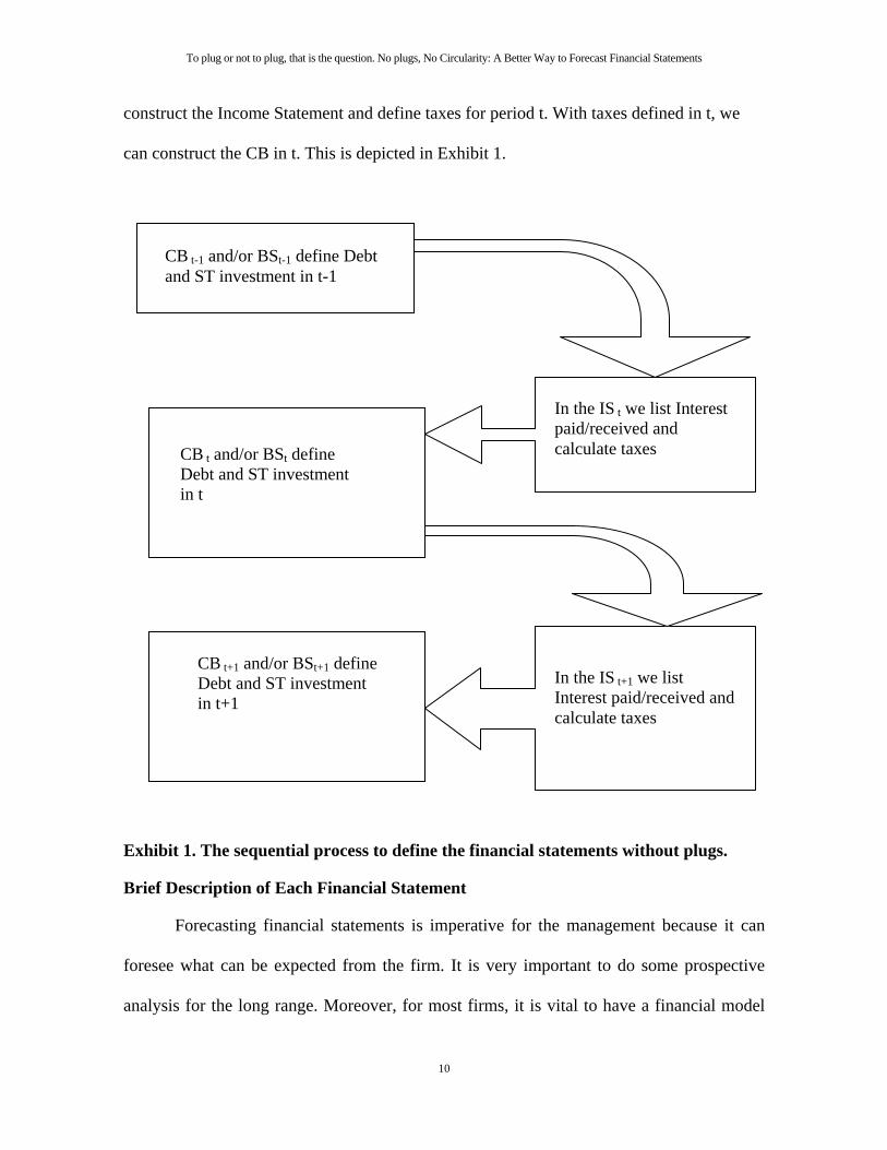
As said above, using the end of period assumption we define the interest

paid/received in any period t having defined debt and short term investment in the previous

period. With interest paid/received from debt/ST investment from previous period we can

3 The BS can be constructed step by step along with the CB and the IS, but for neatness and clearness in the presentation of this work, we construct the BS after the CB and the IS have been completed.


10

construct the Income Statement and define taxes for period t. With taxes defined in t, we

can construct the CB in t. This is depicted in Exhibit 1.

Exhibit 1. The sequential process to define the financial statements without plugs.

Brief Description of Each Financial Statement

Forecasting financial statements is imperative for the management because it can

foresee what can be expected from the firm. It is very important to do some prospective

analysis for the long range. Moreover, for most firms, it is vital to have a financial model

CB t-1 and/or BSt-1 define Debt and ST investment in t-1

In the IS t we list Interest paid/received and calculate taxes CB t and/or BSt define

Debt and ST investment in t

In the IS t+1 we list Interest paid/received and calculate taxes

CB t+1 and/or BSt+1 define Debt and ST investment in t+1


11

that allows management to control value creation. This can be done constructing cash flows

from the financial statements and having a permanent assessment of the firm value. We

propose to construct three financial statements: Balance Sheet, Income Statement and Cash

Budget without plugs and without circularity.

The Balance Sheet

The Balance Sheet is a list at some instant of the assets and rights that a firm

possesses, debts and short and long term obligations with third parties (Liabilities) and the

difference between the former and the later which is known as Equity or what belongs to

the owners. It is like a snapshot of the firm at a specific moment in time. The first part of

the Balance Sheet is the list of the assets the firm owns. The second part shows the

financing of the assets, this is, the liabilities (debt and any other obligation the firm has) and

owner’s equity.

The Income Statement (IS)

This financial statement estimates the Net Income available to be distributed to the

owners. The Income Statement is constructed on the basis of accrual and cost

apportionment. This means that not all the lines recorded in the IS may be considered as

inflow or outflow of cash. In other words, it lists what is earned and not what is received in

cash.

As the Income Statement is a dynamical financial statement, the generation of rights

and obligations is found there. For instance, when the firm dispatches and invoices the

product sold, it has the right to receive the amount invoiced. When the firm uses resources

(raw material, labor, etc.) it has the obligation to pay for those resources. These rights and

obligations are listed in the BS.


12

The Cash Budget

The Cash Budget (CB) or cash forecast or even cash flow, as many name it, shows

the liquidity of the firm. In other words, shows the amount of cash available or in hand in

each instant of time. In the CB we record all the inflows and outflows of the firm. We can

think of the CB as the financial statements that records all the checkbook transactions in the

firm.

Perhaps the CB is the most important financial statement in the firm. With it we can

estimate the financing needs and the cash surplus in every period. In contrast with the IS,

the CB shows the expected occurrence of the cash movements. It shows in addition, the

cumulated balance of cash in the firm. This cumulated balance should be identical to the

line for cash in the Balance Sheet.

Some typical items in the Cash Budget Statement are4:

Inflows

Sales on cash Accounts receivables recovery Loans received Equity invested Inflows from loans lent to third parties Interest received from loans to third parties Sale of inventories Sale of fixed assets Sale of other assets Interest on marketable securities Redemption of marketable securities Customers' in advance payments Value added tax (VAT)

Outflows Payment of Accounts payable and advance payments to third parties Salaries and fringe benefits Principal and interest payments Rent Overhead expenses Promotion and advertising expenses Asset acquisition Social Security payments Taxes (Income, capital gains, VAT) Earnings distributed or dividends paid Investment in marketable securities Repurchase of equity Loans lent to third parties

With this tool we can answer some questions such as, when do we need funds? How

much money do we need? Can we obtain it speeding up the collection of Accounts

Receivable (AR) from customers? Is there a limit in the amount of sales? Can we postpone

4 Taken and adapted from Tham and Vélez-Pareja 2004.


13

some payments? Can we renegotiate the debt terms with the bank? Can we increase sales

with the available resources? For how long can we increase the sales with the actual

available resources? If we increase sales, how much funds do we need to “response” to that

sales effort? How can we negotiate a debt schedule profile with the bank? Which is the

maximum debt capacity of the firm in a given planning horizon? When and how much

liquidity we will have?

It might be thought that our proposal requires extra work. That is true. We need an

extra financial statement: the Cash Budget that is similar to the Cash Flow Statement, but

more detailed. However the time we consume in constructing it is highly profitable for

financial analysis and control. The CB provides a powerful tool for the financial manager.

With the upcoming of low cost computing resources there is no excuse to construct this

financial statement. The idea of working only with the traditional IS and BS was very good

before the personal computer was in the market. Today is a very common resource even for

small and medium size enterprises (SME).

For convenience, we can organize the CB in modules according to the type of

transactions we record.

Detailed description of the CB

It is convenient to organize the CB in five modules as follows:

1. Module 1: Operating activities. 1.1. Operating inflows (basically sales revenues) 1.2. Operating outflows (raw material, labor costs, taxes, overhead

expenses, sales expenses, etc.) 1.3. Net Cash Balance before investment in fixed assets.5

2. Module 2: Investment in assets: 2.1. Initial investment in assets.

5 With this first NCB we could estimate the debt capacity of the firm. If we discount this NCB with the expected cost of debt, we will have the maximum amount the firm can pay during the forecasting horizon.


14

2.2. Investment in assets in other periods. 2.3. Net cash balance of investment in assets. 2.4. Net cash balance after investing in assets.

3. Module 3: External financing. 3.1. Inflow of loans in local or foreign currency (converted to local

currency) 3.2. Principal payment of loans (local or foreign currency) 3.3. Interest paid for local or foreign currency loans. 3.4. Net cash balance of financing.

4. Module 4: Transactions with owners. 4.1. Equity investment 4.2. Dividends payment 4.3. Repurchase of equity. 4.4. Net cash balance of transactions with owners. 4.5. Net cash balance for the year after previous transactions

5. Module 5: Discretionary transactions. 5.1. Inflow from redemption of short term securities 5.2. Interest from market securities. 5.3. Investment in market securities. 5.4. Net cash balance of discretionary transactions. 5.5. Net Cash Balance for the period 5.6. Cumulated cash balance.

The reason of the organization for the CB is related to the construction of cash flows

for valuing the firm using the direct method (See Tham and Vélez-Pareja, 2004, Vélez-

Pareja, 2007, Vélez-Pareja and Tham, 2009).

This step is the crux of the issue. We cannot construct the Income Statement IS, if

we have not previously defined the amounts to be borrowed and the excess cash to be

invested. If we construct the Cash Budget CB, for year 0 we will know the amount of debt

and the amount of excess cash to be invested. In any financial forecast with the initial

information collected (input data) we can construct the IS up to Earnings before Interest

and Taxes, EBIT. In order to move forward, we need to know the return from the excess

cash invested, and the loans contracted if any. With this information we can calculate the

Earnings before Taxes line and estimate the value of taxes. On the other hand, with the IS

for year 1 constructed, we will be able to construct the CB for year 1. Then in general, we

go from CB for year n to IS for year n+1 and then we construct the CB for year n+1 and so


15

on. This is for the case of a new firm/project. In the case of an ongoing concern, we have

the short term investment and the debt in the last historical BS.

Section Three

Problems with the plug

Using plugs poses a problem for forecasting of financial statements: if the analyst

makes a sort of mistakes, the use of the plugs does not help to identify these mistakes

because it always shows that the BS is balanced or matched. This means that one of the

main advantages of the double entry accounting is lost. Next we show an example where

modeling errors are made but not detected by the plug. In doing it we reproduce the look of

a spreadsheet with the columns and rows and the formulas for one period.

Assume we have a firm with the basic input data shown in Table 1:

Table 1. Input data for Example of using plugs A B C D E

1 Corporate tax rate 40% 2 Gross Margin 17.00% 3 Depreciation 1.00 4 Cost of debt (per month) 2.0% Per month 5 Initial equity investment 60.0 6 Sep Oct Nov Dec 7 Sales forecast 124.0 140.0 143.0 167.08 Administrative and sales expenses 4.70 4.70 4.70 4.709 Debt schedule 10 Beginning balance 61.0 60.0 59.0 58.011 Principal payment 1.0 1.0 1.0 1.012 Interest 1.22 1.20 1.18 1.1613 End of year balance 60.0 59.0 58.0 57.0

In table 2 we show two financial statements: the Balance Sheet, BS, and the Income

Statement, IS. The idea with the plug is to match the BS and this is done calculating the

difference between Assets and Liabilities and Equity. Observe in the BS that the plug is

cash.


16

Cash = Total liabilities and equity (C37) minus Accounts Receivable (C18) minus

Inventory (C19) minus Net fixed assets (C24). (2)

This difference is “plugged” in the cell for Cash. In other words, Cash is defined as

a difference, not as the result of inflows and outflows.

Table 2 Balance Sheet with plug in Cash and Income Statement A B C D E F

15 Sep Oct Nov Dec Formula for column C16 Assets 17 Cash (The plug!) 224.2 219.4 227.1 217.7 =C37-C19-C18-C24 18 Accounts Receivable 124.0 140.0 143.0 167.0 =C42 19 Inventory 102.9 116.2 118.7 138.6 =C43 20 Current Assets 451.1 475.6 488.8 523.3 =SUM(C17:C19) 21 Fixed assets 22 Equipment 50.0 50.0 50.0 50.0 =B22 23 Cumulated depreciation 9.0 10.0 11.0 12.0 =B23+C46 24 Net fixed assets 41.0 40.0 39.0 38.0 =C22-C23 25 Total Assets 492.1 515.6 527.8 561.3 =C20+C24 26 Liabilities 27 Accounts payable 102.9 116.2 118.7 138.6 =C43 28 Unpaid taxes 5.7 6.8 7.0 8.6 =C50 29 Debt 60.0 59.0 58.0 57.0 =C13 30 Total Liabilities 168.6 182.0 183.7 204.2 =C27+C28+C29 31 32 Equity 33 Initial equity investment 60.0 60.0 60.0 60.0 =B33 34 Retained Earnings 263.5 273.7 284.1 297.1 =B34+C51 35 Total Equity 323.5 333.7 344.1 357.1 =C33+C34 36 37 Total Liabilities and Equity 492.1 515.6 527.8 561.3 =C30+C35 38 Check 0.0 0.0 0.0 0.0 =C37-C25 41 Sep Oct Nov Dec Formula for column C42 Sales revenues 124.0 140.0 143.0 167.0 =C7 43 Cost of goods sold 102.9 116.2 118.7 138.6 =C42*(1-$C$2) 44 Gross Income 21.1 23.8 24.3 28.4 =C42-C43 45 Administrative and sales expenses 4.7 4.7 4.7 4.7 =C8 46 Depreciation 1.0 1.0 1.0 1.0 =$C$3

47 Earnings before Interest and Taxes

15.4 18.1 18.6 22.7 =C44-C45-C46

48 Interest paid 1.22 1.20 1.18 1.16 =C12 49 Earnings before Taxes 14.2 16.9 17.4 21.5 =C47-C48 50 Tax 5.7 6.8 7.0 8.6 =C49*$C$1 51 Net Income 8.5 10.1 10.5 12.9 =C49-C50


17

In this example we assume that taxes are accrued in the period and paid in the next

one. We can see this observing that unpaid taxes for every period are identical to the tax

accrued in the same period in the Income Statement. The Net Income is cumulated as

Retained Earnings, which means that there is no distribution of dividends.

Observe that the value of accounts payable (C27) and inventory (C19) are defined

as the COGS (C43) in the Income Statement. This is a flagrant violation of the double entry

principle of accounting and yet, the BS matches and balances. The error is to consider that

the COGS is at the same time COGS and inventory. This is a modeling and accounting

mistake when constructing the financial model. This modeling and conceptual error might

be seen as a silly mistake, that is not made by an experienced modeler but it happens.

This example has been taken from a real case, but has been simplified. The main

issue is that when using plugs (as in this simple example), we can incur in many kinds of

errors and the Double Entry Principle will be of no help to detect it. The plug disguises any

mistake we can make and will show that the BS matches.

In tables 3a and 3b we show a sensitivity analysis with the Inventory and Accounts

Receivable AR for October. For different levels of Inventory and AR we observe that the

checking for matching the BS remains no matter which arbitrary amount we use for the two

mentioned cells. The same is done with Total Assets and Total Liabilities and Equity. In

short, we can make any mistake in those lines and the matching will be valid.

Table 3a Sensitivity analysis. Plug maintains the balance: Check cell, AR and Inventory Check Inventory 0.0 0.123 100.000 116.536 130.000AR 0.12345 0.0 0.0 0.0 0.0 100.0 0.0 0.0 0.0 0.0 140.405 0.0 0.0 0.0 0.0 150.0 0.0 0.0 0.0 0.0


18

Table 3b Sensitivity analysis. Plug maintains the balance: Total assets, AR and Inventory Total assets Inventory 515.16 0.123 100.000 116.536 130.000AR 0.12345 515.6 515.6 515.6 515.6 100.0 515.6 515.6 515.6 515.6 140.405 515.6 515.6 515.6 515.6 150.0 515.6 515.6 515.6 515.6From these tables we can observe the following:

1. In some cells (not the plug cell) we can write by mistake any value and the

financial statements show that the basic accounting equation holds.

2. We could make mistakes in modeling the spreadsheet (as seen above) and

the plug will keep the balancing.

3. The same happens with the cells in the liabilities side of the balance. The

total assets (total liabilities and equity) change, but the matching will be

kept.

4. The only consequence in using plugs in the financial model building is not

that the plug disguises the mistakes. These mistakes could affect the

financial planning. In Appendix C we show a simple example where using a

plug a mistake is disguised, but it has consequences in the Income

Statement. The Net Income is wrong and the dividends decisions will be

wrong as well.

5. The above mentioned mistakes occur not only when the model is ready. The

most critical moment is when we are constructing the model. This is, if we

start constructing the model with the plug defined, we will not be able to

know when to stop and conclude that the model is ready for use. Since the

beginning, the plug will say that the model is correct. The other way around,

if we do not include the plug since the beginning and at the end we enter the


19

plug, we will not know if the model is correct because the plug will say that

it is. The plug balances the financial statement. When we do not use plugs

and we are forced to work with the Double Entry Principle, if the financial

statements do not balance we will know that there is something wrong in the

model and we have to go over and double check every step. That is the

beauty of working without plugs.

With this simple example we show some of the problems that could be found when

using plugs to forecast financial statements.

It could be argued that we have to distinguish between endogenous or exogenous

variables. Endogenous ones are not variables in the sense they are the result of a

formulation of the model. Exogenous variables are input variables and if the model is

correctly constructed, will not generate any kind of inconsistency or error. What might

happen with exogenous variables is that results might make no sense. For instance, if we

predict one period inflation rate of 1% and the next an inflation rate of 100%. The results

will be consistent, but not credible.

Section Four

An Example of Forecasting Without Plugs and Without Circularity6

This example deals with a startup firm but the same principles could be used for an

ongoing concern. The example is based on some input data and from them we derive the

complete financial model. We start with an initial CB (year 0) and calculation of loans and

cash excess for investment. We present a detailed explanation of the formulation for

6 This example is presented complete in Appendix A with the spreadsheet formulation in order the reader could construct it by herself. In the body of this work we only forecast two years.


20

calculating debt and cash excess. These explanations include the Excel formulas related to

the financial model we use in the work. We construct the debt schedule for the initial loan.

Some assumptions

1. A startup firm (starting from zero).

2. Taxes are paid the same year as accrued

3. All the expenses and sales are paid and received on a cash basis.

4. Dividends are 100% of the Net Income of previous year.

5. Dividends are paid the next year after the Net Income is generated.

6. Any deficit is covered by new debt.

7. Deficit in the operating module (Module 1) should be covered with short term loans.

Short term loans will be repaid the following year.

8. Deficit in the investment in fixed assets module (Module 2) should be covered with

long term loans. Long term loans are repaid in 5 years.

9. Any cash excess above the targeted level is invested in market securities.

10. In this example we only consider two types of debt: one long term loan and short

term loans (for illustration purposes).

11. Short term portion of debt is not considered in the current liabilities.

Now we present in Table 4 the input data for our financial model


21

Table 4. Input data. B C D E F

4 Input data 5 Equity investment 25.0 6 Long term (LT) Loan 1 at (years) 5.0 7 8 Policies and goals Year 0 1 2 9 Minimum cash required 10.0 10.0 10.0

10 Return of short term investment 8.0% 8.0% 11 Cost of debt, Kd, 13.0% 13.0% 12 EBIT 5.0 9.0 13 Depreciation 9.0 9.0 14 EBITDA = EBIT + Depreciation 14.0 18.0 15 Net fixed assets 45.0 36.0 27.0

For simplicity, we assume no taxes. With this input data we construct the CB for year 0.

Initial CB (year 0) and calculation of loans and cash excess for investment.

Now we present a detailed explanation of the formulation for calculating debt and

cash excess. With the above input data we can construct the CB for year 0. In this way we

define if we have excess cash to invest in short term investments. In the case of a deficit we

will contract a loan.

In order to arrive to the value of the loan to be contracted and to the amount of

excess cash to be invested we have to construct a logical formula in the spreadsheet. The

interesting thing is that we have two referents in calculating the amount of loans: one is the

Net Cash Balance, NCB before investing in fixed assets, Module 1 (in this case it is an

operating NCB and if a deficit exists, it should be financed with short term loans) and the

other is the NCB for investing in fixed assets, Module 2 and this deficit, if exists, should be

covered with long term debt.

In table 5 we show the CB for year 0 in order to calculate the amount of debt and

cash excess investment for forecasting the IS for year 1.


22

Table 5 Cash budget for year 0 to calculate the amount of the loan (independent calculation. No plug! No circularity!)

B C D 17 Cash Budget Year 0 18 Module 1: Operating activities

19 Operating Net Cash Balance NCB (EBITDA)

20 Module 2: Investment in assets

21 Purchase of fixed assets 45.0 =D15

22 NCB of investment in assets -45.0 =-D21

23 NCB after investment in fixed assets -45.0 =D22+D19

24 Module 3: External financing

25 Inflow of loans

26 ST Loan 10.0 =IF((D19-D9)>0,0,-(D19-D9))

27 LT Loan 20.0 =IF(-(D22+D36)>0,-(D22+D36),0)

28 Payment of loans

29 Principal ST loan

30 Interest ST loan. From Loan Schedule

31 Principal LT loan. From Loan Schedule

32 Interest LT loan. From Loan Schedule

33 Total debt payment.

34 NCB of financing activities 30.0 =D26+D27-D33

35 Module 4: Transactions with owners

36 Initial Invested equity 25.0 =D5

37 Dividends payment. Derived from IS 0.0 =D70

38 NCB of transactions with owners 25.0 =D36-D37

39 NCB for the year after previous transactions 10.0 =D38+D34+D23

40 Module 5: Discretionary transactions

41 Redemption of short term ST investment 0.0 =C42

42 Return from ST investments 0.0 =D10*D40

43 Total inflow from ST investments. 0.0

44 ST investments ==> BS 0.0 =C47+D39+D43-D9

45 NCB of discretionary transactions 0.0 =D43-D44

46 NCB for the year 10.0 =D45+D38+D34+D23

47 Cumulated NCB. ==> BS 10.0 =D46

Now we examine the Short term loan in cell D267.

=IF((D19-D9)>0,0,-(D19-D9)) (3a)

Observe that we use only two different cells in the formula, not four as apparently

appears. The relevant formulation for analysis in words is

ST loan (1 year) = -(Operating Net Cash Balance NCB -Minimum cash required for initial

year) (3b)

7 I wish to thank Denis Margarita Mendoza student from Universidad Tecnológica de Bolívar for her insights and questions on this issue. That helped to clarify the formulation of those cells.


23

Observe that the ST loan refers to any eventual deficit BEFORE investment in fixed

assets. This means that we finance the operating deficits with ST debt. Observe as well that

short term debt is used for covering the deficit we have in year 0 in the operational module

and long term debt when we have a deficit AFTER the investment in assets has been made.

Now we examine the LT loan.

The formulation of the LT loan is in cell D27. Observe that all the items (cells) refer

to the same year we are analyzing (Column D).

=IF(-(D22+D36)>0,-(D22+D36),0) (4a)

In words, we can “see” the formula better.

LT Loan = -(NCB of investment in assets + Initial Invested equity) (4b)

Observe that the LT loan refers to any eventual deficit caused by the investment in

fixed assets and this means that we finance the purchase of the assets with LT debt.

We could model that a portion of the deficit after investment in fixed assets could be

covered with one loan at some term and the remaining deficit with loans at another. Or we

could model that any deficit will be financed only by debt or Y% by debt and (1-Y %) by

equity8.

From year 1 and on, we construct a slightly different formula, but the essence is the

same.

Debt schedule for the initial loan

All ST loans are repaid in one year. In Table 6a and 6b we show the ST and LT

loans and the repayments.

8 In fact, Vélez-Pareja 2008, presents a full model with this possibility.


24

Table 6a ST Loan schedule ST Loan schedule Year 0 1 2 Beginning balance 10.0 ?? Interest payment ST loan 1.3 ?? Principal payments ST loan 10.0 ?? Total payment ST loan 11.3 ?? Ending balance 10.0 ?? ?? Interest rate 13.00% 13.00%

Observe that loan (if any) for year 1 is not known yet. We will know it when we

construct the CB for year 1. Next table shows the LT debt schedule.

Table 6b Debt schedule for LT loan in year zero Year 0 1 2 Beginning balance 20.0 16.0 Interest payment LT loan 2.6 2.1 Principal payments LT loan 4.0 4.0 Total payment LT loan 1 6.6 6.1 Ending balance 20.0 16.0 12.0 Interest rate 13.00% 13.00%

Observe that the ending balance for the LT loan in year 3 is not 0. The long term

loan is repaid in 5 years.

In the following tables we show the complete Cash Budget for year 0 and 1 with

two extra columns. In these columns we show the Excel formulas. We usually show one

year, however, when the formula for the first year is different from the second one, we only

show the two formulas.

Financial Statements Step by Step

After we have constructed the CB for year 0 we can begin to construct the Income

Statement for year 1. Here we will show it step by step as if we were constructing it by

hand. When doing it in a spreadsheet the relationships between the different cells are

established and everything happens in simultaneous form. We will make it in a sequential

form to illustrate the process. With the CB for year 0 we know the amount of debt and short

term investment and hence the interest expenses and the interest or return from the


25

investment from year 1. In this way we can complete the IS for year 1. This is shown in

Table 7.

Table 7 Income Statement Year 1 Year 0 1 Earnings Before Interest and Taxes (EBIT) 5.0 Return (interest) from ST investment 0.0 Interest payments. From Loan Schedule 3.9 Net Income ==> BS 1.1 Dividends payment next year ==> CB 0.0 Cumulated retained earnings 0.0

Observe that we need the Cash Budget (CB) for year 0 in order to complete the IS

for year 1. We need to know the return from the short term investment and the interest

payment to complete the IS. The interest payments come from the previous loan schedules.

Why we cannot construct the financial statements (in particular the IS) for the future

years? Because we do not know if there is cash excess to be invested in short term

investments or the deficit to contract new loans in the current year. This is known after we

construct the CB for year 1. In fact, we do not know the interest received from the

investment hence we do not know the income taxes. The same happens with the interest on

debt. We know how much debt we should contract after the CB for the previous year is

completed.

In the case of dividends we assume that dividends are paid only if there is a positive

Net Income. Dividends are paid next year after generated as Net Income.

Now, in Table 8 we calculate step by step the CB for year 1 as well (we only show

the formulas for year 1).

Table 8 The Cash Budget for year 0 and 1 B C D E

17 Cash Budget Year 0 1 18 Module 1: Operating activities

19 Operating Net Cash Balance NCB (EBITDA) 14.0 =E14


21 Purchase of fixed assets 45.0

22 NCB of investment in assets -45.0 0.0 =-E21

23 NCB after investment in fixed assets -45.0 14.0 =E22+E19

24 Module 3: External financing

25 Inflow of loans

26 ST Loan 10.0 3.9 =IF((D47+E23-E33+E43-E9)>0,0,-(D47+E23-E33+E43-E9))

27 LT Loan 20.0

28 Payment of loans

29 Principal ST loan 10.0 =D26

30 Interest ST loan. From Loan Schedule 1.3 =E51

31 Principal LT loan. From Loan Schedule 4.0 =E60

32 Interest LT loan. From Loan Schedule 2.6 =E59

33 Total debt payment. 17.9 =SUM(E29:E32)

34 NCB of financing activities 30.0 -14.0 =E26+E27-E33

35 Module 4: Transactions with owners

36 Initial Invested equity 25.0

37 Dividends payment. Derived from IS 0.0 0.0 =E70

38 NCB of transactions with owners 25.0 0.0 =E36-E37

39 NCB for the year after previous transactions 10.0 0.0 =E38+E34+E23

40 Module 5: Discretionary transactions

41 Redemption of short term ST investment 0.0 0.0 =D44

42 Return from ST investments 0.0 0.0 =E10*E41

43 Total inflow from ST investments. 0.0 0.0 =E42+E41

44 ST investments ==> BS 0.0 0.0 =D47+E39+E43-E9

45 NCB of discretionary transactions 0.0 0.0 =E43-E44

46 NCB for the year 10.0 0.0 =E45+E38+E34+E23

47 Cumulated NCB. ==> BS 10.0 10.0 =D47+E46

As said above the structure of the formulas is the same. For the short term loan (year

1), cell E26, observe as before, that except the cumulated NCB for year 0 (Column D) all

the items (cells) refer to the same year we are analyzing (Column E).

=IF((D47+E23-E33+E43-E9)>0,0,-( D47+E23-E33+E43-E9)) (5a)

Observe that we use only five cells in the formula. The relevant part of the formula

in words is9

9 We do not include the NCB of investment in assets to make formulation simple and improve the reading. We have eliminated the option of a new LT loan to make the example simple. Strictly, there should be another LT loan for covering any long term deficit (purchase of fixed assets, for instance) and keep valid the idea of financing long term deficit with long term debt.


27

ST loan = -(Previous year Cumulated NCB + Operating Net Cash Balance NCB

after investment in fixed assets – Total Debt Payment + Total Inflow from ST investments -

Minimum cash required) (5b)

We also should explain in detail the formula for cash excess in line 44:

=D47+E39+E43+E41-E9 (6a)

We examine the result of that cell as

ST investment = Cumulated NCB (from previous year) + NCB for the year after

previous transactions + Total Inflow from ST investments - Minimum cash required for the

current year (6b)

Again, observe that except the cumulated NCB for year 0 (Column D) all the items

(cells) refer to the same year we are analyzing (Column E).

The idea in the formula is that when we do not have excess cash there is no

investment in market securities. This will happen only when the minimum cash

requirement is fulfilled and there is some extra cash.

Now, in Tables 9a and 9b, we can update the debt schedules:

Table 9a ST Loan schedule B C D E F

49 ST Loan schedule Year 0 1 2 50 Beginning balance 10.0 3.9 51 Interest payment ST loan 1.3 0.5 52 Principal payments ST loan 10.0 3.9 53 Total payment ST loan 11.3 4.4 54 Ending balance 10.0 3.9 ?? 55 Interest rate 13.00% 13.00%

Observe that a second ST loan is needed in year 1 and is repaid in year 2. The

ending balance for year 2 is not known until we construct the CB for year 2. The long term

debt schedule is the same as before because in the example we defined only one LT loan.

The schedule for LT debt is shown in the next table.


28

Table 9b Debt schedule for LT loan in year zero B C D E F

57 Year 0 1 2 58 Beginning balance 20.0 16.0 59 Interest payment LT loan 2.6 2.1 60 Principal payments LT loan 4.0 4.0 61 Total payment LT loan 1 6.6 6.1 62 Ending balance 20.0 16.0 12.0 63 Interest rate 13.00% 13.00%

Now with this information in Table 10 we construct the IS for year 2. The

information we find in the CB for year 1 that we need for the IS in year 2 is the cash excess

investment (to calculate the return received in year 2) and the interest payment (for any new

debt contracted in year 1 and any previous debt).

Table 10 Income Statement Year 2 Year 0 1 2 Earnings Before Interest and Taxes (EBIT) 5.0 9.0 Return (interest) from ST investment 0.0 0.0 Interest payments. From Loan Schedule 3.9 2.6 Net Income ==> BS 1.1 6.4 Dividends payment next year ==> CB 0.0 1.1 Cumulated retained earnings 0.0 0.0

The interest payments for year 2 come from the previous debt schedules (2.1 + 0.5).

Now we have constructed the IS for year 2, we know the dividends to be paid (or the taxes

not shown in this simple example) and we can construct the Cash Budget for year 2 as well.

This is shown in Appendix A.

Now in order to close the process we construct the BS. This financial statement

could had been constructed step by step with the IS and the CB. However, to gain clearness

and make the reading easier, we have left that for the final closing of the process. Once the

CB and IS are defined, we construct the final BS in table 11.

The Balance Sheet

Now we can present the complete Balance Sheet.


29

Table 11 Balance Sheet Year 0 1

Assets Cash. From CB 10.0 10.0 ST investments From CB 0.0 0.0 Total fixed assets. From Input Data 45.0 36.0 Total 55.0 46.0 Liabilities and equity Short term debt. From Loan Schedule 10.0 3.9 LT Debt. From loan schedule 20.0 16.0 Equity investment. From Input Data 25.0 25.0 Net Income current year. From IS 0.0 1.1 Retained earnings. From IS 0.0 0.0 Total Liabilities and equity 55.00 46.00 Check 0.0 0.0

In the BS we record Cash that comes from the CB (Cumulated Net Cash Balance).

In the same fashion, the short term investments are taken from the CB.

In the liabilities side we record the Equity that has three parts: one related to the

initial equity investment and the other two are the current year Net Income and retained

earnings that were calculated in the last lines in the IS. Observe that dividends declared in

year t are paid in year t+1. Net fixed assets come from the Input Data. As an aid to identify

the source of each item in the BS in the example we present a list where each line in the BS

is related to another financial statement.

1. From Cash Budget

a. Cash for the BS

b. LT Debt for the BS

c. Short term debt for the BS

d. ST investments

2. From Income Statement:

a. Net Income for the BS


30

b. Dividends payments for the CB

c. Retained earnings for the BS

3. From Input Data

a. Operating Net Cash Balance NCB (EBITDA)

b. Purchase of fixed assets

c. Initial Invested equity

d. Earnings Before Interest and Taxes (EBIT)

e. Net fixed assets.

f. Equity investment.

In Table 12 we indicate for the three financial statements where each item comes

from and where it goes to.

Table 12. Linking between different lines in the Financial Statements

Input Data

Intermediate Table

Cash Budget

Loan Schedule

Income Statement

Balance Sheet

Cash Budget

Module 1: Operating activities

Operating Net Cash Balance NCB From From

Module 2: Investment in assets

Purchase of fixed assets From

Module 3: External financing

ST Loan Calculated

LT Loan Calculated

Principal ST loan From

Interest ST loan. From To

Principal LT loan. From

Interest LT loan. From To

Module 4: Transactions with owners

Initial Invested equity From To

Dividends payment. To From

Module 5: Discretionary transactions Redemption of short term ST investment

From

Return from ST investments From From To

ST investments Calculated To

Cumulated NCB. From To

ST Loan schedule


31

Input Data

Intermediate Table

Cash Budget

Loan Schedule

Income Statement

Balance Sheet

Beginning balance From

Interest payment ST loan From To To

Principal payments ST loan To

Ending balance To

LT Loan schedule

Beginning balance From

Interest payment LT loan 1 From To To

Principal payments LT loan 1 To

Ending balance To

Income Statement

Earnings Before Interest and Taxes (EBIT)

From

Return (interest) from ST investment

From

From

Interest payments. From

Net Income To

Dividends payment next year To

Cumulated retained earnings To

Balance Sheet

Cash. From

ST investments From

Total fixed assets. From

Short term debt. From

LT Debt. From

Equity investment. From

Net Income current year. From

Retained earnings. From

To some readers it might seem as if the CB is a plug, but it is not. The model is

based on the double entry principle. Hence, any mistake in the numbers should generate an

unbalance in the BS, as it should be. The reader could check (if she constructs the model,

see Appendix A) that any change (arbitrary) in any of the items included in the CB, IS or

BS (except the LT and ST debt and the ST investment, of course), generates an unbalance

in the BS or in the target cash in the BS and the CB. This happens because our model is

based on the Double entry principle. On the contrary, the purpose of a plug is to avoid that


32

this happens. As this model is constructed without plugs, then any arbitrary change in the

lines of the financial statements will generate an unbalance.

When a plug is included in the model, the analyst assumes that one of the totals

(Total assets or Total liabilities + equity) is the "correct" one and after that she picks one of

the two as the “correct” total and she defines where and what the plug is. This is of course,

rather arbitrary.

The CB is constructed out of the different decisions made by the management (in

the future; we are forecasting). In reality the management finds out a deficit and then makes

the decision to finance it. That is what the model does. But it is not done in an arbitrary

way as the traditional and popular plug does. It is made in such a way that the double entry

is permanently valid and when not (say when the analyst makes a mistake or write an

arbitrary number in any of the lines in the financial statements) the double entry system

warns her that she has made a mistake, as it is supposed to happen in any consistent

accounting system. In the traditional and textbook plug approach, it does not warn the

analyst that there is a mistake because it apparently is based on the double entry, and it is

not. It is not in the sense that the financial modeler assumes that she has made no mistakes

and as the double entry is valid, hence cash = total liabilities + equity - non cash assets, for

instance. Making mistakes is very easy even for experts. If the modeler uses plugs from the

start how does she know that there has not been a mistake? Nobody makes mistakes on

purpose. Or, if the modeler does not use plugs from the beginning then the BS will not

match, how will she know that the mismatching is not caused by a mistake? Is it only

because she assumedly was extremely careful in constructing the model? We never know.

This simple example is available on request where we show how to reconcile the

plug approach and the proposed approach after constructing some adjustments and


33

including some extra logical statements. The conclusions from this very simple example

are:

1. The CB is not a plug

2. The model with no plug is constructed with the double entry principle

3. With the model with no plug we can differentiate between LT and ST debt

4. With the model with no plug we can include the ST investment in the BS

5. In the model with no plug we have the correct BS (the correct total assets

without negative cash or negative debt).

6. In the model with no plug ANY arbitrary entry (mistake) is caught by the

model, with the plug it is impossible.

7. No circularity (iterations) is needed.

Some Criticisms to the No Plug No Circularity Approach

Some criticism has been received against this approach. Let us present them and try

to answer every objection.

“The question is whether this is an improvement”.

This is an improvement that can be put in practice using a shorter period of time,

say one month. Actual spreadsheets (Excel 2007, for instance) have more than 16,000

columns. If we wish we could forecast on a daily basis and yet have more than 44 years.

We think that avoiding circularity is a great improvement for complex models.

Circularity often prevents to fulfill the Monte-Carlo Simulation, or it takes a huge time to

simulate the model with a lot of cycle references. We know it on our own experience.

However, we should say this: we are not against circularity per se. Sometimes we need

circularity because it is really needed, for instance, when calculating the Weighted Average


34

Cost of Capital, WACC or Ke, the cost of equity. Our advice is keep circularity as few as

possible for the above mentioned reasons. See Vélez-Pareja and Benavides, 2006. The use

of no plug is undoubtedly an improvement because we propose and give a methodological

approach to avoid the use of plug that as has been said, is like sweeping the dirt under the

carpet and we can conceal many modeling and accounting errors.

Using the end of year assumption for defining the interest charges over longer periods, such as a year, will likely lead to less accurate results than when using the average loan assumption to compute interest expense

The main advantage of using the end of period assumption is that it is consistent

with the valuation techniques that assume an end of period approach for calculating WACC

(for instance). But all depends on how we estimate the cost of debt, Kd (See Appendix D

for an example). It is not recommended to use the contractual Kd precisely because what

happens “within” the period (a year). When constructing the pro forma financial statement

we have either the debt schedule and the cost of debt for each loan OR we can make an

estimation of historical Kd as described in (Vélez-Pareja, 2009) (for simplicity assume that

market value of debt is its book value). If we start estimating historical Kd as (Financial

Expensest FEt)/Debtt-1 for consistency we will model the interest charges as Kdt×Debtt-1,

this is, we would follow the end of year convention. Hence, the need for circularity

vanishes. In the above mentioned work we show that using the sum of interest to estimate

Kd ((Financial Expensest FEt)/Debtt-1) and the end of year assumption the averaging

approach gives a lower value for the interest payments and consequently for the tax shields.

Which method is best depends on the user. The approach focuses on internal financial analysts. That group has access to a large amount of data and this can lead to rich‐featured financial models. On the other hand, external analysts have much more limited data availability. External analysts, such as commercial lenders, are better served by the average loan convention.


35

The explanations and answer to the previous criticism on the end of period approach

is precisely suited for external analysts. We agree that external analysts have much less

information than internal. No doubt. However, we find external analysis somehow

nonsensical precisely because there is a lack of information and we have to make a lot of

assumptions. It might be preferable to work with the internal analyst and put the looking

glass on her assumptions and inputs. If we construct the financial statements WITHOUT

plugs or circularity, it will be crystal clear for any expert and the external expert will not

need to make heroic assumptions.

The suggested advantage is that your procedure is more accurate than the plug approach because it can eliminate modeling errors. While it can eliminate modeling inconsistencies, it doesn’t avoid problems caused by unreasonable assumptions (nor does the plug method). It is true that the plug approach can hide modeling errors if the user assumes that the plug is correct because the balance sheet balances, and then blindly uses the result. However, we teach our students that after they “balance the balance sheet” with the plug they should do error checking. This includes visual inspection of the results, and analysis of common size income statements and financial ratios for the projected income statements and balance sheets. Our experience is that this procedure effectively identifies problems.

The unreasonable assumptions have no place in this discussion because that is not

inherent to any modeling approach. For us modeling errors are model construction or

conceptual errors. On the other hand, if you put garbage in, you will get garbage out

(remember: GIGO). How can we check for error if the plug doesn’t tell you that there exists

an error? You have two options: start the modeling process without the plug and you

introduce the plug when YOU THINK the model is error free (but the BS is not matching

and it tells you that there is at least an error) and then use the plug. Or you can start using

the plug BUT you never will know that there is an error. When do you stop the modeling

without the plug and introduce it if the BS doesn’t match? Remember that still you either

have an error in case of not matching or you have solved the mismatching in case it


36

matches and you don't need the plug. In the other case, if the BS matches with the plug,

when do you stop the search for errors? Which is the signal or protocol that tells the

modeler the model is done? This is like a conundrum.

When using no plugs and the BS matches, in rigor, we cannot say the model is

100% free of errors. There might be compensating errors and still the BS matches.

HOWEVER, if the BS doesn’t match WE DO KNOW that there is an error and we have to

find it out. When using plugs we ARE NOT aware that an error exists because the BS

always matches. The situation is very simple: The BS is either matched or not. If the first,

you don’t need the plug. If the second, you have an error and using the plug is to hide the

error. Vélez-Pareja and Hurtado (2007) list many mistakes students and analysts make

while modeling the forecast for financial statements. They look silly when you have found

them, BUT they were a headache before that. The process of finding errors takes much

more time than the construction of the model itself.

The other factor to consider is cost. The recommended approach is more complex and time consuming to construct than the plug approach. The question is whether the benefit is worth the cost.

Well, if you think that for every case you have to start from scratch, the cost is high.

We agree. However, that is not what happens in consulting and inside a firm or even in an

external situation. Once you have constructed your model, you can use it over and over and

you can “polish” and sophisticate it. We have been working on this model for decades and

right now we use a (huge) model in consulting that covers many possible scenarios. We

don’t need to model every case from scratch. We estimate that the crux of our model relies

on few cells: short and long term debt and equity investment and excess cash to be invested

in short market securities. A more complex model than the one we describe in this work

and that the reader can download can be constructed (as you notice, we give the formulas)


37

in about four hours of careful work. Is that too expensive for a firm? Will our students with

a 3 credit course have the time to do it?

The Cash Budget is a plug In Appendix B we show the two way tables where we include changes in different

items from the financial statements and the unbalancing in each case. This is an indication

that the CB is not a plug. If it were, the balancing would be kept for each change.

Section Five

Concluding remarks: no plugs, no circularity

We have shown a way to teach better the forecasting of financial statements. We

have described the experience of using models without plugs and circularity in the

classroom. Evidence of successful results was given.

In this work we have illustrated in a simple manner and step by step the way to

construct consistently three forecasted financial statements: the Cash Budget, the Income

Statement and the Balance Sheet. This process has taken into account the interaction among

the financial statements in such a way that the figures from one financial statement are

included in other(s). As we have shown, we do not need to include plugs, neither to iterate

for solving circularity. The procedure is based on the double entry principle.

In financial modeling, it is common to use plugs in the construction of the balance

sheet. With plugs, we specify that the balance sheet will match, even if there are mistakes

in the derivation of the non-plug items. In other words, there is no external protocol to

check the consistency of the balance sheet.

In our model, we follow the double entry principle in forecasting financial

statements and derive the balance sheet. The double entry principle provides a consistency

check for the balance sheet.


38

If the balance sheet does not match, then we know that there are errors in the model.

If the balance sheet matches, the model might still have errors but the probability of errors

cancelling each other is lower than with the plug approach.

The model we propose follows the double entry principle. Our reasoning is: when

we construct a model to forecast financial statements we should keep valid the double entry

principle. It is possible to make mistakes (accounting or modeling mistakes) and that

principle warns us about those possible mistakes. If we make one of such mistakes there is

an indication of it because the Balance Sheet does not match. When the BS matches we

estimate that the probability of errors or mistakes canceling out on a 100% basis is too low

and we assume that the model is correct.

On the contrary, when we use plugs we assume that we do make no mistakes when

constructing the model and hence, because the double entry principle should be kept, any

difference or mismatching in the BS totals can be plugged-in in the line used as plug.

Hence, the BS will match when adding/subtracting that difference.

An approach like this might be seen as too elaborated and costly. However, as said

above, analysts do not need to start from zero every time: once the model is built, it can be

used over and over. This approach allows the management to apply sensitivity analysis,

scenario management and Monte Carlo Simulation enriching the decision making process.

This type of tools is very useful in crisis times when we have to manage the firm with a

scalpel and not with an ax.

Bibliographic References

Arnold, Tom M. and Peter Charles Eisemann, 2007, "Debt Financing Does Not Create a Circularity within Pro Forma Analysis" (February 26). Available at SSRN:


39

http://ssrn.com/abstract=965547 Benninga, Simon, 2007, Conference: Teaching of Finance with Excel, Guest Speaker in 4th

National and 1st International Symposium for the Teaching in Finance, Cartagena, June 20. ISSN 1900-3218.

Benninga, Simon, 2006, Principles of Finance with Excel, Oxford, London. Brealey, Richard A., Stewart C. Myers and Alan J. Marcus, 1995, Fundamentals of

Corporate Finance, McGraw-Hill. Daves, Phillip R., Michael C. Ehrhardt and Ronald E. Shrieves, 2004, Corporate

Valuation: A Guide for Managers and Investors, Thomson. Day, Alastair L., 2001, Mastering Financial Modeling. A Practitioner’s Guide to Applied

Corporate Finance, Prentice Hall, London. English, James, 2001, Applied Equity Analysis. Stock Valuation Techniques for Wall Street Professionals, McGraw-Hill. Gallagher, Timothy J. and Joseph D. Andrew, jr., 2000, Financial Management 2nd ed.,

Prentice Hall. Google Search on August 2nd, 2007 for “plug forecasting financial statements”:

http://www.google.com.co/search?hl=es&q=plug+forecasting+financial+statements&btnG=Buscar&meta=

Higgins, Robert C., 2001, Analysis for Financial Management, 6th ed. Irwin-McGraw-Hill. Horngren, Charles T., Gary L. Sundem John A. Elliott, Donna Philbrick, 2005, Introduction

to Financial Accounting (9th Edition). Prentice-Hall. Hurtado, Dary Luz, 2008, Corporación Universitaria DLHC, Proyecciones de estados

financieros 2008 - 2018, Accountancy Department, Universidad Tecnológica de Bolívar. Course Project Ingeniería Económica. Available at http://cashflow88.com/decisiones/PROYECCIONES_2008-2017.xls

Kester, George W., 1987. A Note on Solving the Balancing Problem, Financial Management, Vol. 16, No. 1 (Spring), pp. 52-54

Palepu, Krishna G., Paul M. Healy and Victor L. Bernard, 2004, Business Analysis & Valuation. Using Financial Statements, Thomson.

Penman, Stephen H, 2001, Financial Statement Analysis & Security Valuation, McGraw-Hill – Irwin.

Polimeni, Ralph S., Frank J. Fabozzi, and Adelberg, A. , 1991. Cost Accounting Concepts and Applications for Managerial Decision Making. McGraw-Hill.

Ross, Stephen A., Randolph W. Westerfield and Jeffrey Jaffe, 1999, Corporate Finance, 5ª edición, Irwin-McGraw-Hill.

Tham Joseph and Ignacio Vélez Pareja, 2004, Principles of Cash Flow Valuation. An Integrated Market Based Approach, Academic Press.

The Happy Accountant. http://happyaccountant.wordpress.com/2007/07/03/advantages-of-double-entry-bookkeeping/ (Visited on July 23, 2007)

Tjia, John S. 2004, Building Financial Models. A Guide to Creating and Interpreting Financial Statements. McGraw-Hill, New York.

Van Horne, J.C. 2001, Financial Management and Policy, 12th Ed., Prentice Hall Inc., Englewood Cliffs, New Jersey.

Vélez Pareja, Ignacio, 2008, A Step by Step Guide to Construct a Financial Model without Plugs and without Circularity for Valuation Purposes. (June 1, 2008). The paper is available at SSRN: http://ssrn.com/abstract=1138428).


40

Vélez Pareja, Ignacio, 2007a. Decisiones de inversión. Para la valoración de proyectos y de empresas, Universidad Javeriana, Politécnico Grancolombiano. Bogotá.

Vélez-Pareja, Ignacio, 2007b. "Guidelines for Forecasting Financial Statements from Historical Financial Statements for Valuation Purposes (Updated)" (July 13, 2007). Available at SSRN: http://ssrn.com/abstract=872474

Velez-Pareja, Ignacio, 2009, Which Cost of Debt Should be Used in Forecasting Cash Flows? (Updated)(March 15). Estudios Gerenciales, Vol. 24, No. 110. Forthcoming April/June 2009. Available at SSRN: http://ssrn.com/abstract=1011485

Velez-Pareja, Ignacio and Benavides Franco, Julián, 2006, There Exists Circularity between Wacc and Value? Another Solution (November 12, 2005). Estudios Gerenciales, Vol. 98, pp. 13-23, January-March 2006. Available at SSRN: http://ssrn.com/abstract=846804

Vélez-Pareja, Ignacio and Joseph Tham, 2009, Prospective Analysis: Guidelines for Forecasting Financial Statements in en S.R. Vishwanath, C. Krishnamurti (eds.), Investment Management: A Modern Guide to Security Analysis and Stock Selection, DOI: 10.1007/978-3-540-88802-4 2, © 2009 Springer-Verlag Berlin Heidelberg, ISBN: 978-3-540-88801-7. Available at SSRN at http://papers.ssrn.com/abstract=1026210 (October, 2007).


41

Appendix A

In this Appendix the reader finds the simplified model presented in the body of the work. We indicate the formulas that have to be

utilized in the construction of the financial model. We have constructed the formulas in such a way that they can be used to construct part of

or the complete model. In the first line and in the first column we have written the letters and numbers corresponding to the Excel®

spreadsheet in order to make it easier the localization and the construction of the different formulas. In the last two columns we have written

those formulas. Usually the formulas correspond to the year 0 and/or year 1. Shaded cells are for the input data.

Construct the model trying to understand why we use the different cells that appear in the formula and do not make this construction as

a typing exercise. In Table A1 we present the input data.

Table A1. Input data B C D E F G

Year 0 1 2 3 3 4 Input data 5 Equity investment 25.0 6 Long term (LT) Loan 1 at (years) 5.0 7 8 Policies and goals Year 0 1 2 3 9 Minimum cash required 10.0 10.0 10.0 10.0

10 Return of short term investment 8.0% 8.0% 8.0%11 Cost of debt, Kd, 13.0% 13.0% 13.0%12 EBIT 5.0 9.0 12.013 Depreciation 9.0 9.0 9.014 EBITDA 14.0 18.0 21.015 Net fixed assets 45.0 36.0 27.0 18.0

With this input information we can construct the CB in table A2.


42

Table A2 Cash Budget B C D E F G

17 Year 0 1 2 3 0 1

18 Module 1: Operating activities

19 Operating Net Cash Balance NCB (EBITDA) 14.0 18.0 21.0 =E14


21 Purchase of fixed assets 45.0 =D15 22 NCB of investment in assets -45.0 0.0 0.0 0.0 =-D21 =-E21 23 NCB after investment in fixed assets -45.0 14.0 18.0 21.0 =D22+D19 =E22+E19 24 Module 3: External financing 25 Inflow of loans

26 ST Loan 10.0 3.9 0.0 0.0=IF((D19-D9)>0,0,-(D19-D9))

=IF((D47+E23-E33+E43-E9)>0,0,-(D47+E23-E33+E43-E9))

27 LT Loan 20.0 =IF(-(D22+D36)>0,-(D22+D36),0) 28 Payment of loans 29 Principal ST loan 10.0 3.9 0.0 =D26 30 Interest ST loan 1.3 0.5 0.0 =E51 31 Principal LT loan 4.0 4.0 4.0 =E60 32 Interest LT loan 2.6 2.1 1.6 =E59 33 Total debt payment. 17.9 10.5 5.6 =SUM(E29:E32) 34 NCB of financing activities 30.0 -14.0 -10.5 -5.6 =D26+D27-D33 =E26+E27-E33 35 Module 4: Transactions with owners 36 Initial Invested equity 25.0 =D5 37 Dividends payment 0.0 0.0 1.1 6.4 =D70 =E70 38 NCB of transactions with owners 25.0 0.0 -1.1 -6.4 =D36-D37 =E36-E37 39 NCB for the year after previous transactions 10.0 0.0 6.4 9.0 =D38+D34+D23 =E38+E34+E23 40 Module 5: Discretionary transactions 41 Sale of short term ST investment 0.0 0.0 0.0 6.4 =C42 =D44 42 Return from ST investments 0.0 0.0 0.0 0.5 =D10*D40 =E10*E41 43 Total inflow from ST investments. 0.0 0.0 0.0 6.9 =E42+E41 44 ST investments ==> BS 0.0 0.0 6.4 16.0 =C47+D39+D43-D9 =D47+E39+E43-E9 45 NCB of discretionary transactions 0.0 0.0 -6.4 -9.0 =D43-D44 =E43-E44 46 NCB for the year 10.0 0.0 0.0 0.0 =D45+D38+D34+D23 =E45+E38+E34+E23 47 Cumulated NCB 10.0 10.0 10.0 10.0 =D46 =D47+E46

There is an interaction between CB and the debt schedule. In Tables A3 and A4 we show the debt schedules for the loans defined in

the previous table.


43

Table A3 ST Loan schedule B C D E F G H I 49 Year 0 1 2 3 0 1 50 Beginning balance 10.0 3.9 0.0 =D54

51 Interest payment ST loan 1.3 0.5 0.0 =D54*E55

52 Principal payments ST loan 10.0 3.9 0.0 =D54

53 Total payment ST loan 11.3 4.4 0.0 =SUM(E51:E52)

54 Ending balance 10.0 3.9 0.0 0.0 =D26 =E50-E52+E26

55 Interest rate 13.00% 13.00% 13.00% =E11

Table A4 LT Loan schedule B C D E F G H I

57 Year 0 1 2 3 =D62

58 Beginning balance 20.0 16.0 12.0 =E63*E58

59 Interest payment LT loan 1 2.6 2.1 1.6 =($D$62)/$D$6

60 Principal payments LT loan 1 4.0 4.0 4.0 =E59+E60

61 Total payment LT loan 1 6.6 6.1 5.6 =D27 =E58-E60

62 Ending balance 20.0 16.0 12.0 8.0 =E11

63 Interest rate 13.00% 13.00% 13.00% =D62

Now we present in Table A5 the Income Statement. Table A5 Income Statement

B C D E F G =D46 =E46 65 Year 0 1 2 3 0 1 66 Earnings Before Interest and Taxes (EBIT) 5.0 9.0 12.0 =E12 67 Return (interest) from ST investment 0.0 0.0 0.5 =E10*D44 68 Interest payments. From Loan Schedule 3.9 2.6 1.6 =E59+E51 69 Net Income ==> BS 1.1 6.4 11.0 =E66+E67-E68 70 Dividends payment next year ==> CB 0.0 1.1 6.4 =D69 71 Cumulated retained earnings 0.0 0.0 0.0 =D71+D69-E70

Finally, in Table A6 we show the complete Balance Sheet. Note that when constructing

the financial model we have to temporarily link some cells with no data (or formula in it) and the

temporal results will not coincide with the value shown in the tables. The final results will be

seen when the model is finished.

Table A6 Complete Balance Sheet B C D E F G =D62 =E62

74 Year 0 1 2 3 0 1 75 Assets 76 Cash. From CB 10.0 10.0 10.0 10.0 =D47 =E47 77 ST investments From CB 0.0 0.0 6.4 16.0 =D44 =E44 78 Total fixed assets. From Input Data 45.0 36.0 27.0 18.0 =D15 =E15 79 Total 55.0 46.0 43.4 44.0 =D78+D76+D77 =E78+E76+E77 80 Liabilities and equity 81 Short term debt. From Loan Schedule 10.0 3.9 0.0 0.0 =D54 =E54 82 LT Debt. From loan schedule 20.0 16.0 12.0 8.0 =D62 =E62 83 Equity investment. From Input Data 25.0 25.0 25.0 25.0 =D5 =D80+E35 84 Net Income current year. From IS 0.0 1.1 6.4 11.0 85 Retained earnings. From IS 0.0 0.0 0.0 0.0 =D68 =E71 86 Total Liabilities and equity 55.00 46.00 43.41 43.95 =SUM(D81:D85) =SUM(E81:E85) 87 Check 0.0 0.0 0.0 0.0 =D86-D79 =E86-E79

Next we show how the different lines of the financial statements are interrelated.


44

Appendix B

How the changes affect the non plug, no circularity model.

What we show in this Appendix is that when changing some values (either by

constructing a mistaken model or introducing by error a number instead of a formula in the

model), the Double entry Principle shows an unbalancing check. The tables work identifying a

couple of values (independent variables) and looking the value in the body of the table. Use the

Data option in the spreadsheet.

Using items from the CB in the previous model, in Tables B1 and B2 we construct two

way tables and show how any arbitrary change in two items will show a non matching (non

checking) in the BS. Observe that it matches for the values we have in the original model.

Table B1 Checking and changes in Initial Assets and Equity in year 2 in the CB Check yr 2 Initial Assets 0.0 0.0 15.0 20.0 45.0 10.0 -30.0 -15.0 -10.0 15.0 Initial equity in CB 25.0 -45.0 -30.0 -25.0 0.0 30.0 -50.0 -35.0 -30.0 -5.0 35.0 -55.0 -40.0 -35.0 -10.0

In the same fashion, when we analyze for Dividends and ST investments.

Table B2 Checking and changes in ST loans and Principal payment of LT loan in year 2

Check yr 2 Dividends payment yr 2

0.0 0.0 1.0 1.1 2.0 0.0 -1.1 -0.1 0.0 0.9 ST investments yr 2 5.0 -6.5 -5.5 -5.4 -4.5 10.0 -11.9 -10.9 -10.8 -9.9

Conclusion: The CB IS NOT A PLUG! In the same fashion when using items from the

IS and the BS, we can show that the balancing is lost.


45

Appendix C

How a Concealed Error Might affect Critical Results

When we use plugs the consequences are not only that they disguise mistakes of several

classes. It might lead to bad decisions. In the next tables we show a simple example using plug

and we show that the mistakes we incur on and not detected could affect decisions such as

dividend decisions. In Table C1 we show the input data for a simple example.

Table C1. Input data B C D E F G

3 Year 0 1 2 3 4 Input data 5 Equity investment 25.0 6 Long term (LT) Loan 1 at (years) 5.0 7 8 Policies and goals Year 0 1 2 3 9 Minimum cash required 13.0 11.0 16.0 19.0

10 Return of short term investment 8.0% 8.0% 8.0%11 Cost of debt, Kd, 13.0% 13.0% 13.0%12 EBIT 5.0 9.0 12.013 Depreciation 9.0 9.0 9.014 EBITDA 14.0 18.0 21.015 Net fixed assets 45.0 36.0 27.0 18.0

In Table C2 we present the Income Statement showing the formulas to be constructed to build the model. Table C2. The Income Statement

B C D E F G 17 Income Statement Year 0 1 2 3 1 18 Earnings Before Interest and Taxes (EBIT) 5.0 9.0 12.0 =E12 19 Return (interest) from ST investment 0.0 0.0 0.1 =IF(D32>0,0,-D32*E10) 20 Interest payments 2.6 2.1 1.6 =D33*E11 21 Net Income 2.4 6.9 10.5 =E18+E19-E20 22 Cumulated retained earnings 2.4 6.9 10.5 =E21

Now we show in Table C3 the Balance Sheet with a plug in short term debt.


46

Table C3. The Balance Sheet B C D E F G

25 Balance Sheet Year 0 1 2 3 0 26 Assets 27 Cash CB 13.0 11.0 16.0 19.0 =D9 28 ST investments CB 29 Total fixed assets IT 45.0 36.0 27.0 18.0 =D15 30 Total 58.0 47.0 43.0 37.0 =D29+D27+D28 31 Liabilities and equity 32 Short term debt 13.0 3.6 -0.9 -6.5 =+D30-D33-D34-D35 33 LT Debt CB 20.0 16.0 12.0 8.0 20 34 Equity investment ID 25.0 25.0 25.0 25.0 =D5 35 Retained earnings IS 0.0 2.4 6.9 10.5 =D22 36 Total Liabilities and equity 58.00 47.00 43.00 37.00 =SUM(D32:D35) 37 Check 0.0 0.0 0.0 0.0 =D36-D30

Now in Table C4 we show how the plug in the model shows that the financial statements match,

but the mistake in long term debt (not detected because the use of plug shows that there exists

balancing), results in lower Net Income (and lower dividends distribution.

Table C4. Two way table showing balancing and change in Net Income.

NI1 NI2 NI3 check 1 check 2 check 3 2.4 6.9 10.5 0.0 0.0 0.0 5 4.4 8.5 11.6 0.0 0.0 0.0 10 3.7 8.0 11.2 0.0 0.0 0.0 15 3.1 7.4 10.8 0.0 0.0 0.0 LT debt yr 0 20 2.4 6.9 10.5 0.0 0.0 0.0 25 1.8 6.4 10.3 0.0 0.0 0.0 30 1.1 6.1 10.2 0.0 0.0 0.0 35 0.6 5.9 10.0 0.0 0.0 0.0


47

Appendix D

How to Calculate Kd for a Non Plug, No Circularity Model.

In this Appendix we show an example on how to calculate Kd from historical data and following the end of period convention.

When making an estimation of historical Kd (this is a real life case and financial data are taken from the financial statements of a firm traded at the stock market. For simplicity and for the purpose of illustration we will assume that market value of public debt is its book value) follow the next procedure:

1. Start estimating historical Kd as Kd =FEt/Debtt-1. This step takes into account what happens during t.

2. We assume CAPM and say Kd = Rf + Risk Premium. Hence, we estimate Risk Premium, RP, as Kd-Rf. For forecasting we assume the RPforecast as an average of historical.

3. We estimate a real interest rate as (1+Rf)/(1+infl)-1 and use the historical average for forecasting it. (We could use a longer period of time for estimating ireal if we wish).

4. Then we have the inputs for estimating Rf for the forecast. Rfforecast=(1+inflforecast)x(1+ireal)-1.

5. Now we forecast Kd as Rfforecast + RPforecast. 6. Now, when modeling we can (moreover, we have to) follow the end of period convention

for estimating interest charges and therefore, circularity is avoided without any inconsistency and eventually, without any under or over estimation.

7. When the forecast is done, we will estimate Kd for each forecast period as (Interest paymentt)/Debtt-1. This way we will be consistent all the way down and we could use the traditional textbook formula for the WACC (if all conditions to use it are fulfilled). Remember that tax savings, TS, are based on what you actually list as an interest expense and on the timing of tax payment. At the end, the correct Kd to be used in the WACC (regarding the TS) is the one that arises from calculating the interest rate as (Interest paymentt)/Debtt-1.

8. For consistency we will model the interest charges as Kdt×Debtt-1, this is, we would follow the end of year convention. Hence, the need for circularity vanishes.

Carulla-Vivero 2004 2005 2006 2007 2008

Average to be used as forecast

2009 forecast

2010 forecast

Total debt (St and LT) 271.283,02 281.618,13 350.524,32 226.046,10 222.008,00Financial expenses, FE 23.516,50 33.663,03 35.894,51 40.504,26 34.163,31Kd =FEt/Debtt-1 12,4% 12,7% 11,6% 15,1%Risk free rate, Rf 11,10% 9,10% 6,60% 7,20% 8,50%Debt Risk Premium = Kd -Rf

3,31% 6,15% 4,36% 6,61% 5,11% 5,11% 5,11%

Inflation rate 5,50% 4,90% 4,50% 5,70% 7,70% 5,57% 4,53%Real rate 5,31% 4,00% 2,01% 1,42% 0,74% 2,04% 2,04% 2,04%Rf 7,73% 6,67%Kd = Rf+ Debt Risk Premium

12,83% 11,77%

Then what happens when you use (say) the traditional textbook formula for WACC (Kd×(1-T)×D%t-1 + Ke×E%t-1) and plug in the contractual Kd? You will have an interest payment that is not calculated based on the end (beginning) of period assumption, your TS will be different from the actual forecasted TS and your value calculations will be inconsistent.

Forecasting Financial Statements with No plugs and No Circularity ...

Documents

Transcript of Forecasting Financial Statements with No plugs and No Circularity ...