Forecasting Economic Activity for Estonia
130
Forecasting Economic Activity for Estonia Dissertation Zur Erlangung des Doktorgrades Dr. rer. pol. Im Fach Volkswirtschaftslehre Unter der Leitung von Professor Dr. Michael Funke Eingereicht an der Universität Hamburg Fachbereich Volkswirtschaftslehre (VWL) Von Diplom-Volkswirt Christian Schulz Hamburg, 2008
Transcript of Forecasting Economic Activity for Estonia

Forecasting Economic Activity for Estonia
Dissertation
Zur Erlangung des Doktorgrades
Dr. rer. pol.
Im Fach Volkswirtschaftslehre
Unter der Leitung von
Professor Dr. Michael Funke
Eingereicht an der
Universität Hamburg
Fachbereich Volkswirtschaftslehre (VWL)
Von Diplom-Volkswirt Christian Schulz
Hamburg, 2008

- 2 -
Angenommen vom Fachbereich Volkswirtschaftslehre (VWL) der Universität Hamburg
Prüfungsausschussvorsitzender: Prof. Dr. Peter Stahlecker
1. Gutachter: Prof. Dr. Michael Funke
2. Gutachter: Prof. Dr. Thomas Straubhaar
Datum der Prüfung: 30. Oktober 2008

- 3 -
Table of Content
INTRODUCTION (pages 1 – 9)
PART I: Forecasting Economic Growth for Estonia: Application of Common
Factor Methodologies (Pages 1 – 47)
PART II: Forecasting Economic Activity for Estonia: Application of Dynamic
Principal Components Analysis (Pages 1 – 36)
PART III: Can Inflation Help in Determining Potential Output of the Estonian
Economy? (Pages 1 – 36)
- 4 -
INTRODUCTION
Of the many tasks economists undertake, forecasting is possibly one of the most relevant to
decision makers in practice. Indeed, many of the other tasks like modelling, explaining and
estimating economic relationships only become relevant to a wider public when the results are
employed to the prediction of certain variables of interest. These variables in macroeconomic
forecasting range from the development of sales and profits in certain product markets to
price and inflation forecasting and forecasting of economic activity for individual regions,
countries, groups of countries, or indeed the whole world. As policymakers and investors
must rely on macroeconomic forecasts when making both short-term and long-term decisions,
much effort and resources have been spent on the development and application of forecasting
tools.
Since the beginning of the 20th century macroeconomic forecasts are increasingly derived
from economic models and employ leading indicators as well as econometric and statistical
methods (Clements and Hendry, 2000). With these, researchers try to fulfil various
requirements made of forecasts, for instance:1
- Accuracy: Forecasts should be quantitative and accurately predict the forecasted
variable as well as stating the expected forecasting error
- Timeliness: Forecasts should take account of the most up-to-date information and not
be subject to revisions later on
- Stability: The forecasting model’s performance must be stable with respect to changes
in the environment, such as economic regime shifts
Macroeconomic forecasting based on business cycle theory was founded by Burns and
Mitchell (1946), who had also played a significant role in the founding of the first
independent institutions which started to publish economic forecasts regularly. The National
Bureau of Economic Research (NBER) in the United States was founded as early as 1920.
One of the first popular leading indicators, the Harvard Barometer, was introduced in 1919,
based among others on the work of Persons (1919). In Europe, pioneers of model based
forecasting worked in the Netherlands, where Tinbergen’s macroeconomic models started to
be used in the 1930s, strengthened later by the works of Theil (1966). The variety of
1 Cf. Zarnowitz (1992)

- 5 -
published leading indicators worldwide has grown constantly since, with new developments
in the conceptual and methodical frameworks, but also with the failings of established
indicators in warning of imminent economic crises (indeed, the Harvard Barometer had failed
to predict the great recession in 1929). In addition to econometrically derived indicators,
survey-based indicators became more and more popular, such as the IFO Institute of
Economic Research index in Germany, which is a survey of business sentiment among
managers of a large and representative sample of firms of the economy. Today, a plethora of
published leading and coincident indicators is available for every country, at least for the
mature western economies.2
The object of the forecasting exercises in this work is the economy of Estonia. This small
country, the northernmost of the three Baltic republics, declared independence from the
Soviet Union in 1991. The second Estonian republic (the first independence had only lasted
from 1918 till 1940) immediately made a rapid transition from the Soviet planned economy to
a very liberal market economy. The successful transition process finally led to Estonia’s
accession to both NATO and the European Union in 2004. The economic catch-up process of
Estonia can be divided into three phases. During the first phase, which began immediately
after independence and the painful rupture with the old planned-economy system, economic
growth accelerated quickly, supported by strictly laissez-faire policies of the government, a
stable currency-board exchange rate regime and the proximity to and support of its
Scandinavian neighbours. This positive development came to a sudden halt when the Russian
economic crisis of the late 1990s hit Estonia, leading to a brief but marked recession in
1998/1999. This was the second economic phase. During this recession the last remains of
Estonia’s connections to the old Soviet area broke down and a firm orientation towards the
Northern and Western European economies took place. The third phase started after the
Russian crisis and its aftermath, with the new millennium. Economic growth picked up again
quickly and stayed between 5% and 7% for the first half of the current decade. During this
period, inflation remained relatively stable and low, and unemployment, which had been
chronically high during the 1990s, steadily declined. In 2006 and 2007 economic growth
attained double-digits once again. This, in conjunction with other indicators such as a very
high current account deficit, rising inflation and very high property prices signalled
2 It should be mentioned that the discussion of whether economic forecasts are possible and, if so, successful, is
as old as the development of the methods itself, starting with Morgenstern (1928).

- 6 -
overheating in the Estonian economy. The current discussion in Estonian economic circles is
about whether or not Estonia can avoid a “hard landing”. However, most indicators and the
most recent (spring 2008) forecasts of the Bank of Estonia point towards exactly this
unwelcome development.3
The focus of the studies assembled in this paper is the application of different unobserved
common factor models to the forecasting of economic activity in Estonia. In the first two
papers, common factor methodologies are used to extract leading indicators from large panels
of macroeconomic data. The resulting leading indicators are then used to forecast economic
activity. The third paper focuses on the growth potential of the Estonian economy and
employs common factor methodology to extract a cyclical component in GDP from two
equations: an output equation and a Phillips curve equation. This permits the calculation of
the varying inflation non-accelerating growth rate of the economy, or its potential growth rate.
The first paper is entitled “Forecasting Economic Growth for Estonia: Application of
Common Factor Methodologies” and presents the application of two different unobserved
factor models to an Estonian data set: state-space modelling and static principal components.
It thereby extends the methodologies currently used by the Bank of Estonia for short-term
forecasting to include the use of common factor methodologies. State-space modelling was
introduced to economic forecasting by Stock and Watson (1991). The idea is that a common
dynamic trend is extracted from a small set of potentially leading variables, which excludes
much of the idiosyncratic movements of the individual series. State-space modelling is used
to describe the dynamic framework, the coefficients of which are subsequently estimated
using Kalman filtering techniques. The result is a single leading indicator that can then be
tested for its predictive capacity. Static principal components are widely used and have, for
instance, been applied by Stock and Watson (2002) to economic forecasting. It is an efficient
method for deriving common factors from a large set of data. The idea is to derive
components that explain the largest part of the cross-sectional variance. Therefore, static
principal components are based on the variance-covariance matrix of a data set and can easily
be computed using any standard econometric software package. In the paper, first, the
respective common factors are derived; second, the forecasts of real economic growth for
Estonia are performed and, finally, evaluated against benchmark models for different
estimation and forecasting periods. In-sample testing (Diebold and Mariano, 1995) and out-
3 The latest spring forecast 2008 of the Bank of Estonia can be found on its website at www.eestipank.info .

- 7 -
of-sample testing (Clark and McCracken, 2001) is employed. The results demonstrate that
both methods show improvements over the benchmark model, but not for all forecasting
periods. This paper was published as Working Paper 09/2007 in the Bank of Estonia Working
Paper Series.
The second paper’s title is “Forecasting Economic Activity for Estonia: Application of
Dynamic Principal Components Analysis”. In this paper, we apply a method developed by
Forni, Hallin, Lippi and Reichlin (2000) to derive a short-term leading indicator for economic
activity in Estonia. This method was initially developed for and applied to Euro zone data
(Forni et al., 2001). There are three main advantages to the method: First, it allows the
efficient use of large panels of economic time series; there are many economic time series
available for Estonia, however compared to the data available for most Western countries, the
length of the time series is rather short. The use of large panels therefore increases the total
information available. Second, the method permits the derivation of one or a few common
factors which can be used for forecasting; the information contained in the large panel of data
is condensed into only one leading indicator based on the “common” components of the time
series, i. e. cleansed of their idiosyncratic components. And third, the method allows for
discrimination between series as leading or lagging with respect to economic activity at
relevant frequencies; dynamic principal components methodology lets us look at measures of
coherence at relevant cycle lengths. In the paper we find that indeed the derived leading
indicator, which is a combination of the common components of twelve leading time series,
outperforms alternative forecasting models. Both in-sample testing and pseudo out-of-sample
testing indicate clear improvements over benchmark models.
The second paper pays additional attention to the correct specification of growth cycles in
Estonia. We find that a particularly good way to do this is to use a three-state Markov
switching model similar to the one used by Hamilton (1989). Estonia has been in a true
recession (by Western standards) only once in the aftermath of the Russian crisis in the late
1990s. Before and after, however, growth has shifted between periods of sustainable growth
(particularly during the five years following the Russian crisis) and periods of booming and
probably unsustainable growth (just before the Russian crisis and since 2005). This
endogenous cycle dating method seems to yield better results than the popular Bry and
Boschan (1971) cycle dating method used by the American National Bureau of Economic
Research (NBER). This paper was published as Working Paper 02/2008 in the Bank of
Estonia Working Paper Series.

- 8 -
The third and final paper is entitled “Can Inflation Help in Determining Potential Output of
the Estonian Economy?” and applies a common factor model developed by Kuttner (1994) to
the identification of output gaps and the potential output of the Estonian economy. The central
idea of the model is to combine a simple output equation and a Phillips curve equation for
inflation, linking the two via a transitory or cyclical component of output. The assumption is
that this cyclical component drives inflation, a result we would expect from a theoretical point
of view (Okun, 1962). It can therefore be seen as a hybrid between purely statistical filtering
methods such as the Hodrick-Prescott filter or bandpass filtering à la Baxter and King (1999)
and models with strong theoretical foundations, such as the production function approach
(Perry, 1977) used by the European commission. The model, originally developed for the U.S.
economy, has to be adapted to the small and open Estonian economy and the catch-up process
it has gone through. The paper presents alternative specifications for the Phillips curve and
compares the results. Estimation results, diagnostics and sensivity tests show that a model
which includes foreign direct investment as a weakly exogenous variable in the output
equation and a traditional Phillips curve relationship with wage inflation (rather than
consumer price inflation or the GDP deflator as in other applications) as the dependent
variable provides the best results. The resulting series for potential growth shows marked
differences from the other widely-used models for the identification of output gaps.4 This
stems from the development of inflation rates in Estonia over the sample period. Inflation
rates were very high during the 1990s, particularly up until the Russian crisis. Similarly to
more mature economies, inflation rates then fell to very low levels in the early 2000s before
they started to rise strongly again from 2005 onwards. This results in high negative output
gaps before the Russian crisis and low positive output gaps after it. The output gap grows as
actual output growth remains below potential output growth for some years. Only at the very
end of the sample do we observe negative output gaps again as inflation climbs. The paper
shows that the resulting estimates outperform the Hodrick-Prescott filter in terms of pseudo
real-time reliability, according to tests developed by Planas and Rossi (2004).
4 Cf. Kattai and Vahter (2006)

- 9 -
Baxter, M. and King, R. G. (1999). Measuring Business Cycles: Approximate Band-Pass
Filters for Economic Time Series. The Review of Economics and Statistics 81 (4), 575-
593.
Burns, A. F. and Mitchell, W. C. (1946). Measuring Business Cycles. New York: National
Bureau of Economic Research.
Clark, T. E. and McCracken, M. W. (2001). Tests of Forecast Accuracy and Encompassing
for Nested Models. Journal of Econometrics 105, 85-110.
Clements, M. P. and Hendry, D. F. (2000). Forecasting Economic Time Series. Cambridge:
Cambridge University Press.
Diebold, F. X. and Mariano, R. S. (1995). Comparing Predictive Accuracy. 13Journal of
Business & Economic Statistics, 253-263.
Forni, M., Hallin, M., Lippi, M. and Reichlin, L. (2001). Coincident and Leading Indicators
for the Euro Area. The Economic Journal, 62-85.
Forni, M., Lippi, M. and Reichlin, L. (2000). The Generalized Factor Model: Identification
and Estimation. The Review of Economics and Statistics 82, 540-554.
Kattai, R. and Vahter, P. (2006). Kogutoodangu Lõhe ja Potentsiaalne SKP Eestis. mimeo.
Kuttner, K. N. (1994). Estimating Potential Output as a Latent Variable. Journal of Business
& Economic Statistics 12, 361-368.
Morgenstern, O. (1928). Wirtschaftsprognose: Eine Untersuchung ihrer Voraussetzungen und
Möglichkeiten. Wien: Springer.
Okun, A. (1962). Potential GNP: Its Measurement and Significance. In Proceedings of the
Business and Economic Statistics Section of the American Statistical Association.
Perry, G. L. (1977). Potential Output: Recent Issues and Present Trends. In U.S. Productive
Capacity: Estimating the Utilization Gap. Working Paper, Washington University:
Center for the Study of American Business.
Persons, W. M. (1919). An Index of General Business Conditions. The Review of Economic
Statistics 1(2), 111-205.
Planas, C. and Rossi, A. (2004). Can Inflation Data Improve the Real-Time Reliability of
Output Gap Estimates? Journal of Applied Econometrics 19, 121-133.
Stock, J. H. and Watson, M. W. (1991). A Probability Model of the Coincident Economic
indicators. In Leading Indicators: New Approaches and Forecasting Records(Eds,
Lahiri, K. and Moore, G. H.). Cambridge, UK: Cambridge University Press, 63-89.
Stock, J. H. and Watson, M. W. (2002). Forecasting Using Principal Components from a
Large Number of Predictors. Journal of the American Statistical Association 97, 147-
162.
Theil, H. (1966). Applied Economic Forecasting. Amsterdam: North Holland Publ. Co.
Zarnowitz, V. (1992). Business Cycles - Theory, History, Indicators and Forecasting.
Chicago: University of Chicago Press.

Working Paper Series
9/2007
Eesti Pank Bank of Estonia
Forecasting Economic Growth
for Estonia:
Application of Common Factor
Methodologies
Christian Schulz


Forecasting Economic Growth for Estonia:
Application of Common Factor
Methodologies
Christian Schulz
Abstract
In this paper, the application of two different unobserved factor mod-
els to a data set from Estonia is presented. The small-scale state-space
model used by Stock and Watson (1991) and the large-scale static prin-
cipal components model used by Stock and Watson (2002) are employed
to derive common factors. Subsequently, using these common factors,
forecasts of real economic growth for Estonia are performed and evalu-
ated against benchmark models for different estimation and forecasting
periods. Results show that both methods show improvements over the
benchmark model, but not for the all the forecasting periods.
JEL Code: C53, C22, C32, F43
Keywords: Estonia, forecasting, principal components, state-space model,
forecast performance
Author’s e-mail address: [email protected]
The views expressed are those of the author and do not necessarily represent
the official views of Eesti Pank.

Non-technical summary
The forecasting of economic growth draws a lot of attention in all countries
and new methods are constantly being developed to improve the performance
of forecasting models. While all of these methods are universally applicable
in principle, their appropriateness for particular settings has to be examined.
As more and more macroeconomic time series data becomes easily available,
there has been a shift in the development of these methods towards the inclu-
sion of more time series into the forecasting models. One promising field is
the study of unobservable common factors in large data sets, where the as-
sumption is made that a small number of factors drive the whole data set and
that the use of these factors can improve forecasts.
In this paper we apply two different methods to extract common factors
from an Estonian data set of quarterly macroeconomic time series from 1994
to 2006. One is a small-scale state-space model which has been used by Stock
and Watson (1991) for economic forecasting. This model is estimated using
maximum likelihood and a Kalman filter procedure. As the number of time
series variables, which can be included in this model, is small, it requires
careful pre-selection. We use different specifications of the model, each based
on three time series. To represent specificities of the Estonian economy, we
include survey type data such as industrial order books as well as financial
data such as monetary supply and stock exchange data. The latter two reflect
the fact that our analysis suggests that financial data are more relevant for
forecasts of the Estonian economy than other authors have found for many
mature economies.
The second methodology we apply draws on the principal components lit-
erature. Following Stock and Watson (2002), we use a static principal compo-
nents model based on a large data set of 34 time series, which represent a large
part of the total available data set. This method is computationally rather sim-
ple and is computed for a contemporaneous data set and a “stacked” data set.
The latter includes the first lags of the 34 time series to allow for the existence
of phase shifts. This analysis yields several factors which can be interpreted
with respect to the influence individual time series have upon them.
We follow a large part of the literature on forecasting in concluding with the
evaluation of our resulting forecasting models compared to a benchmark naïve
model. In-sample comparisons and out-of sample comparisons are presented.
The latter uses a sub-sample of the whole data set to estimate the forecasting
equation and then uses the remainder of the sample to evaluate and compare
the performance.
The in-sample forecast evaluation according to Diebold and Mariano (1995)
shows that our models outperform the naïve forecast for most of the evalua-
2

tion periods, particularly for the period of the Russian crisis in the late 1990s.
However, this outperformance is not always significant and particularly for
the end of the sample most models are actually worse than the naïve forecast.
The out-of sample tests according to Clark and McCracken (2001) show that
the additional information included in our models is not statistically irrelevant,
however. The naïve model does not encompass our forecasting models.
Overall, common factor models do improve forecasts and reveal a lot of
information about the underlying data set, particularly for the principal com-
ponents approach.
3

Contents
1. Introduction . . . . . . . . . . . . . . . . . . . . . . . . . . . . . . 5
2. Specific features of the Estonian economy . . . . . . . . . . . . . . 6
3. Identification of leading time series . . . . . . . . . . . . . . . . . . 13
4. Common factor methodologies . . . . . . . . . . . . . . . . . . . . 17
4.1. The state-space model . . . . . . . . . . . . . . . . . . . . . . 17
4.2. Static principal components . . . . . . . . . . . . . . . . . . . 24
5. Forecast comparison . . . . . . . . . . . . . . . . . . . . . . . . . 33
6. Conclusions . . . . . . . . . . . . . . . . . . . . . . . . . . . . . . 37
References . . . . . . . . . . . . . . . . . . . . . . . . . . . . . . . . . 39
Appendix 1. Data set and cross correlations . . . . . . . . . . . . . . . 42
Appendix 2. Principal components: time series included . . . . . . . . 45
4

1. Introduction
The Estonian economy has been growing quickly since the country re-
gained its independence in the early nineties and this growth has recently in-
creased to double digits, vastly exceeding the potential of 5–7% defined by
the Bank of Estonia. Being able to make accurate predictions about such high
growth rates is extremely relevant for policy makers and is pursued by sev-
eral institutions both in Estonia and internationally. This paper extends the
methodology currently used by the Bank of Estonia for short-term forecasting
to include the use of common factor methodologies; namely, state-space dy-
namic common factor models and principal components analysis. We focus
research on the prediction of economic growth, but similar models can also be
used to forecast inflation or other macroeconomic variables.
State-space modelling was introduced to economic forecasting by Stock
and Watson (1991). The idea is that from a small set of potentially leading
variables a common dynamic trend is extracted, which excludes much of the
idiosyncratic movements of the individual series. State-space modelling is
used to describe the dynamic framework, the coefficients of which are sub-
sequently estimated using Kalman filtering techniques. The result is a single
leading indicator that can then be tested for its predictive capacity. Principal
components analysis comes in two different forms — static and dynamic. Sta-
tic principal components are widely used and have, for instance, been used by
Stock and Watson (2002) for economic forecasting. It is an efficient method
for deriving common factors from a large set of data. The idea is to derive com-
ponents that explain the largest part of the cross-sectional variance. Therefore,
static principal components are based on the variance-covariance matrix of a
data set and can easily be computed using any standard econometric software
package. Dynamic principal component methodology for economic forecast-
ing was developed by Forni et al. (2000). It is based on the spectral density
matrix of a data set and requires more specific software. We leave this applica-
tion to future research. Obviously, evaluating the performance of the derived
leading indicators requires some attention as well. We will use in-sample and
out-of-sample tests to evaluate the performance of these indicators.
The remainder of this paper is laid out as follows. Section 2 takes a closer
look at some of the specific features of the Estonian economy which need to be
taken into account when constructing forecasts. In Section 3, we take a look
at the data set and preliminarily analyse its predictive powers. In Section 4,
we use dynamic common factor analysis following Stock and Watson (1991)
to construct a leading indicator and evaluate its performance. In Section 5,
the static principal components model is presented and a leading indicator is
derived. This is then evaluated and compared to other forecasting models. Our
5

conclusion is presented in Section 6.
2. Specific features of the Estonian economy
In this section we will focus on two aspects of the Estonian economy that
may be important when trying to forecast future economic growth. One as-
pect is the existence of cycles, specifically growth cycles that may help when
making forecasts. The other aspect is how the Estonian economy differs from
other economies.
If we want to predict the economic situation in Estonia, we first have to
look at its growth pattern over the period we can consider. To avoid the early
transition pains encountered by Estonia as it struggled to shake off Soviet in-
fluence, we start in the first quarter of 1995. Another reason for beginning
there is that the data before this period is only partially available and of some-
times questionable quality. At this time, we use the GDP time series as they
were published before 2006. In 2006, major changes were made in the collec-
tion and calculation methodologies as part of the harmonisation process with
EU standards. This update changed GDP levels by up to 6.0%, according to
the Annual Report 2006 of Statistics Estonia, and growth figures, which are
more relevant to this paper, changed somewhat as well. Unfortunately, only
data from 2000 onwards is currently available under the new methodology.
This time span is too short for the methodologies we employ later on. There-
fore, we must link the old and new data before the longer time series under the
new methodology is set and published by the Statistics Office of Estonia later
this year.
In the Figure 1 year-on-year-growth (from –4% up to +16%) is presented
on the y-axis. It can be seen that since 2000, growth has fluctuated but has
been positive throughout. Before, there was a brief phase of strong growth
running up until 1998, followed by a sharp decline in growth and even a brief
period of negative growth. It can also be seen that growth has significantly
exceeded the long-term corridor between 5% and 9% since 2005.
In addition to economic growth as such, the reliable signalling of economic
phases or business cycles is often required from forecasts and specifically from
leading indicators. In business cycle analysis, the output gap is commonly
used to identify the current position in the cycle. It represents the current usage
of the production capacity of an economy. Under-usage of capacity indicates
a recession; over-usage indicates a boom, with up- and downswings in be-
tween. The Ifo Institute for Economic Research has found an intuitive graphic
6

-.04
.00
.04
.08
.12
.16
1996 1998 2000 2002 2004 2006
GDP_EST_YOYGR_LINKED
Figure 1: Real GDP Growth in Estonia (% yoy, constant 2000 prices)
way of illustrating the current position of an economy (CESIfo, 2007)1. The
“economic climate clock” plots an indicator of the perception of the current
(or very recent) climate of the economy versus expectations. We do this for
Estonia using the consumer climate indices published by the Estonian Eco-
nomic Institute for the past twelve months (recent climate) and the coming
twelve months (expectations). As the Russian crisis of 1998 clearly marks a
break, we display two different graphs below: one for the period 1995–1999,
the other for 2000–2006 (see Figure 2).
The four quadrants of the “economic clock” have different interpretations
according to the relationship between the expectations and interpretations of
the current situation or recent past. Table 1 represents interpretations for the
different quadrants.
Neither of the two periods exhibits the typical smooth development from
one economic phase to another2. Instead, there seems to be a lot more vari-
ation than we would find in more mature economies. From 1997 to 1998,
the Russian crisis seemed to have taken the Estonian consumers by surprise,
which is why the clock turned from boom to bust within a period of only two
quarters. The second quadrant “downturn” was skipped; the economy dropped
1For further details on the economic clock and examples for Germany, see Nerb (2007).2For examples of mature economies, see Nerb (2007).
7

Source(s): ifo, data: Estonian Economic Institute
-30
-20
-10
0
10
20
30
-35 -25 -15 -5 5 15 25 35
Next 12 months
Last 12 months
1995 – 1999
Boom
DownswingRecession
Upswing
1999:IV
1995:III1995:I
1996:I
1997:I
1998:I
1999:I
Source(s): ifo, data: Estonian Economic Institute
-30
-20
-10
0
10
20
30
-35 -25 -15 -5 5 15 25 35
Next 12 months
Last 12 months
2000 – 2006
Boom
DownswingRecession
Upswing
2000:I
2006:I
2005:I
2004:I
2003:I
2002:I
2001:I
Figure 2: Economic clock — consumer perception of the general economic
situation
8

Table 1: Interpretation of the economic clock figures
Quadrant Perception of past 12 months Expectations of future 12 mths. Interpretation
I Positive Positive Boom in the economy
IV Positive Negative Downswing in the economy
III Negative Negative Recession in the economy
II Negative Positive Upswing in the economy
sharply into recession. At the beginning of the second half of the sample, the
years 2000 and 2001 were still marked by a negative perception of the current
state of the economy, but with improving expectations. The clock moved to
the fourth quadrant “upswing” before entering the “boom” quadrant in 2002.
In 2003, the clock signalled a downswing, which fortunately for Estonia, did
not continue on to become a recession, but rather turned back to a boom in
2005 with the most recent values at record levels. This movement has been
due to the fact that the current state of the economy is persistently seen as pos-
itive and only the expectations shift. However, the negative expectations did
not seem to materialise, which is why the economy reverted to a boom. This
discussion shows that traditional business cycle analysis is unlikely to lead to
the same stable results as in mature economies when applied to an economy
that is still emerging, such as Estonia. It also shows that there have only been
three major cycles: strong and volatile growth until the Russian crisis, a sharp
downturn during the Russian crisis, and strong, rather stable and accelerating
economic growth ever since.
To obtain some sort of formalized view of the existence of cycles, we use
the method developed by Bry and Boschan (1971) for dating business cycles,
but we adapt it to the identification of growth-cycles; that is, cycles in the 4th
differences of GDP. The Figure 3 displays the results.
There are four growth-cycle recessions which can be identified using Bry
and Boschan’s method: 1996:1–1996:4, 1997:2–1999:2, 2001:2–2002:2 and
2006:1-.
In the search for leading indicators for Estonia, attention has to be paid to
the economic specificities of its economy. There are three characteristics that
we will take a closer look at:
• the Estonian economy’s openness to trade,
• important sectors of the economy,
• the importance of foreign direct investment and the role of money sup-
ply.
9

-.04
.00
.04
.08
.12
.16
1996 1998 2000 2002 2004 2006
GDP_EST_YOYGR_LINKED
Figure 3: Growth cycle recessions in Estonia
Estonia is one of the world’s most open economies, with trade (the sum of
imports and exports of goods and services) amounting to almost 160% of the
gross domestic product (see Figure 4). Therefore, when predicting macroeco-
nomic variables for Estonia, special consideration might be taken of variables
that represent the influence of trade on the Estonian economy. It should be
noted, however, that openness seems to be a function of the size of an econ-
omy. This is shown in the following figure, which demonstrates that there is
a negative linear relationship between the size of a country, represented by its
population in Log-terms, and its openness.
Estonia is a very open economy, but it is not an outlier given the relation-
ship above. This is reflected in the fact that we find Estonia above the esti-
mated OLS-regression line, but not dramatically so3. Nonetheless, because of
the importance of trade, we include macroeconomic variables from Estonia’s
important trade partners in the data set. We selected variables from Finland,
the Euro zone and Russia, as these countries and areas comprise Estonia’s
most important trade partners, as can be seen in the Figure 5.
3The negative-sloping regression line shows that generally, in smaller countries, trade
plays a bigger role than in larger ones.
10

0
50
10
0
15
0
20
0
25
0
30
0
35
0
40
0
02
46
81
01
21
41
6
Ln
of
Po
pu
lati
on
Mil
lio
n
Imports and Exports (% of GDP)
Est
on
ia
Ger
man
y
Fig
ure
4:
Op
enn
ess
ver
sus
Po
pu
lati
on
So
urc
e:E
con
om
ist
Inte
llig
ence
Un
it(E
IU).
11

26
.6%
13
.2%
6.2
%
8.7
%
4.6
%
8.8
%
4.7
%
6.0
%
2.4
%
3.5
%
3.3
%
1.2
%
6.5
%
3.7
%
2.4
%
2.3
%
3.4
%
19
.6%
9.2
%14
.0%
Fin
lan
d
Sw
ed
en
Ge
rma
ny
Ru
ss
ian
Fe
de
rati
on
La
tvia
Lit
hu
an
ia
Ne
the
rla
nd
s
Un
ite
d
Kin
gd
om
De
nm
ark
Po
lan
d
Figure 5: Trade partners of Estonia
Source: Statistical Office of Estonia.
The decomposition of GDP by sector yields the Figure 6, which shows both
value added in different sectors and the respective compound annual growth
rates for 1995–2005. All data is in constant year 2000 prices.
3 % -7 % 17 % 6 % 1 % 10 % 11 % 9 % 7 % 4 % 9 % 3 % 2 % 0 % 7 %
Co
mp
ou
nd
an
nu
al g
row
th
rate
1995 -
2005
224
8 20
842
187
458
1290
93
968
292
879
408
262
153
231
Ag
ricu
ltu
re
Fis
hin
g
Min
ing
Man
ufa
ctu
rin
g
Ele
ctr
icit
y s
up
ply
Co
nstr
ucti
on
Wh
ole
sale
, re
tail
trad
e
Ho
tels
an
d r
esta
ura
nts
Tra
nsp
ort
an
d
co
mm
un
icati
on
s
Fin
an
cia
l
inte
rmed
iati
on
Real esta
te
Pu
blic a
dm
inis
trati
on
Ed
ucati
on
Healt
h
Oth
er
Figure 6: Estonian GDP by sectors
Source: Statistical Office of Estonia.
12

The largest sectors are trade (retail and wholesale), transport, real estate
and manufacturing. Growth is spread rather evenly across sectors, with the
secondary sector somewhat underperforming the tertiary sector. These results
do not reveal ex-ante suppositions about possible leading indicators; however,
the eventual choice of variables should be checked against this composition to
avoid the use of economically insignificant variables. This would be the case
for instance, if fishing turned out to be a good leading indicator statistically
(which indeed it does).
Foreign direct investment is important to the Estonian economy for two
reasons. First, it can be seen as a proxy for overall investment. Second, it
is, as Zanghieri (2006) points out, the “only non-debt-creating foreign source
of capital” to finance Estonia’s persistent current account deficit (Zanghieri,
2006:257). There is a considerable amount of literature on the qualities of
financial variables as leading indicators for economic cycles; for instance, Es-
trella and Mishkin (1998) and Fritsche and Stephan (2000). In general, their
findings state that there are only very limited and unstable empirical relation-
ships in developed countries. Yet for Estonia, the particularities of its economy
will lead to different results, as this paper will suggest. This may be due to
Estonia’s monetary regime, the currency board linked with the Deutschmark
(since 1999 with all European currencies and subsequently, the euro).
3. Identification of leading time series
There is a table in the appendix containing all the time series available in
sufficient length and frequency as well as their respective cross-correlation
characteristics with respect to real GDP growth as a reference series4. The
table indicates the transformations made to achieve stationarity, their respec-
tive unit-root-test results (augmented Dickey-Fuller test) and maximum cross-
correlations, and the lag (positive number) or lead (negative number) at which
this maximum cross-correlation is recorded.
In the following section, we will explore the leading or lagging character-
istics of the different types of variables with respect to real GDP growth in
Estonia. The data was categorised into four groups: (1) financial variables, (2)
trade variables, (3) GDP-sector variables and (4) survey-type variables.
The financial variables included in the data set exhibit very different char-
4Using cross-correlations to analyse the lagging and leading characteristics of variables
with respect to each other is standard in the empirical literature — for instance, see Bandholz
and Funke (2003), and Forni et al. (2001). Gerlach and Yiu (2005) use contemporaneous
correlations and principal components to pre-identify variables useful for the construction of
a common factor of economic activity in Hong Kong.
13

acteristics (see Figure 7). As a matter of illustration, they are spread over four
quadrants here with the upper two quadrants indicating significant maximum
correlation coefficients (> 2√T
, equals 0.33 for T=44) and the lower two quad-
rants insignificant correlations. The right-hand side indicates a leading char-
acteristic of the variable with respect to real GDP growth in Estonia, and the
left-hand side indicates a lagging relationship; that is, the graph illustrates at
which lag (or lead) of the explanatory variable the maximum cross-correlation
is achieved.
-1
-0,5
0
0,5
1
-5 -4 -3 -2 -1 0 1 2 3 4 5
Ma
x.
Cro
ss
-c
orr
ela
tio
n
(ab
so
lute
)
Significant Lagging Variables
Significant Leading
Variables
Insignificant Lagging Variables
Insignificant Leading
Variables
0.30T
2±=
Significant Lagging Variables
Significant Leading
Variables
Figure 7: Cross-correlation characteristics of Financial Variables 1995–2006
Source: Statistical Office of Estonia; The Economist Intelligence Unit, European Central
Bank; OECD.
For example, monetary supply (M1 andM2) exhibits a rather strong short-
term leading characteristic, while interest rates seem to be lagging with high
coefficients. The stock exchange indices for emerging markets that we have
included display rather high correlations, yet at very different lags and leads.
We have also included Estonian gold reserves (in national valuation) in the
financial data set, even though they seem to correlate rather weakly with GDP
growth.
Trade variables in the data set exhibit comparatively low maximum cross-
correlations, yet they seem to have leading characteristics in general (see Fig-
ure 8). Finnish and Euro zone variables seem to have the strongest coeffi-
cients, with Finnish exports, Finnish GDP and euro zone GDP “scoring” the
14

-1
-0,5
0
0,5
1
-5 -4 -3 -2 -1 0 1 2 3 4 5
At Lag (negative: Lead)
Ma
x.
Cro
ss
-c
orr
ela
tio
n
(ab
so
lute
)
Significant Lagging Variables
Significant Leading
Variables
Insignificant
Lagging Variables
Insignificant
Leading Variables
0.30T
2±=
Significant Lagging Variables
Significant Leading
Variables
Figure 8: Cross-correlation characteristics of Trade Variables 1995–2006
Source: Statistical Office of Estonia; The Economist Intelligence Unit, European Central
Bank; OECD.
highest. Russian variables, represented here by Russian GDP, exhibit weaker
relationships. It seems that the Estonian economy is more strongly influenced
by its new Western and Northern European partners than by its older Russian
liaisons.
Most of the economic sectors in Estonia seem to have rather coinciden-
tal characteristics in terms of temporality with respect to Estonian GDP (see
Figure 9). In particular, manufacturing displays a very high coincident cross-
correlation. The only strongly short-term leading sectoral variable seems to be
value added in the financial intermediation (banking) sector. Transportation
and retail trade have a more long-term relationship, yet it is less pronounced.
The health sector seems to be lagging, but here the strength of this relationship
is rather low.
The different surveys again exhibit very different patterns (see Figure 10).
Many of them have quite strong relationships with real GDP growth in Es-
tonia. Among the leading variables, we find industrial order books surveys,
industrial confidence, and retail trade confidence. Among the strongly lagging
relationships we find construction order books and construction confidence.
15

-1
-0,5
0
0,5
1
-5 -4 -3 -2 -1 0 1 2 3 4 5
At Lag (negative: Lead)
Ma
x.
Cro
ss
-c
orr
ela
tio
n
(ab
so
lute
)
Significant Lagging Variables
Significant Leading
Variables
Insignificant
Lagging Variables
Insignificant
Leading Variables
0.30T
2±=
Significant
Lagging Variables
Significant
Leading Variables
Figure 9: Cross-correlation characteristics of sectoral variables 1995–2006
Source: Statistical Office of Estonia; The Economist Intelligence Unit, European Central
Bank; OECD.
-1
-0,5
0
0,5
1
-5 -4 -3 -2 -1 0 1 2 3 4 5
Ma
x.
Cro
ss
-
co
rre
lati
on
(a
bs
olu
te)
Significant Lagging Variables
Significant Leading
Variables
Insignificant
Lagging Variables
Insignificant
Leading Variables
0.30T
2±=
Significant Lagging
Variables
Significant Leading
Variables
Figure 10: Cross-correlation characteristics of Survey-Type Variables 1995–
2006
Source: Statistical Office of Estonia; The Economist Intelligence Unit, European Central
Bank; OECD.
16

4. Common factor methodologies
4.1. The state-space model
In this section, we will employ methods originally developed by Kalman
(1960) and Kalman (1963) to estimate a dynamic common factor model and
to construct a leading indicator for the Estonian economy. This approach was
initially also favoured by Stock and Watson (1991). The same methodology
has been used successfully by other authors, for instance, Bandholz and Funke
(2003) for Germany, Gerlach and Yiu (2005) for Hong Kong, and Curran and
Funke (2006) for China.
The dynamic factor model’s main identifying assumption is that the co-
movements of the indicator series (observed variables) arise from one single
unobserved common factor. This factor is expected to provide better forecasts
of the reference series than the individual indicator series. The factor is con-
structed only from the observed series; that is, the reference series — in our
case real GDP growth — is not used in the process. Constructing the com-
mon factor involves (1) formulating the model, (2) converting the model to
state-space representation and (3) estimating the parameters using maximum
likelihood (MLE) methodology, for which the Kalman filter is employed. The
Kalman filter is composed of two recursive stages: (1) filtering and (2) smooth-
ing. Filtering involves estimating the common factor for period t on the basis
of information available at period t − 1. The forecast error is minimised us-
ing MLE. The second stage, smoothing, then takes account of the informa-
tion available over the entire sample period. The algorithm is computationally
rather expensive; that is, achieving the convergence of the different coefficients
and parameters is time-consuming5. Because of this technical restriction, only
a few variables can be included in the model. This requires a careful selec-
tion of the input variables, for which there are numerous criteria. These are
well summarised by Bandholz (2004). Among the formal criteria we find the
following:
• A significant relationship between the lagged leading variable and the
reference series in terms of general fit.
• The stability of this relationship.
• Improved out-of-sample forecasting.
• Timely identification of all turning points to avoid incorrect signals.
5The software we employed was kindly made available by Chang-Jin Kim and is de-
scribed in Kim (1999).
17

Moreover, there are a number of informal criteria which should be looked
at:
• Timely publication.
• High publication frequency
• Not subject to major ex-post revisions.
• Existence of theoretical background for leading relationship.
First, we would like to focus on the discussion of which system of lead-
ing variables might well represent the Estonian economy. For the German
economy, industrial indicators such as order books are used as manufacturing
plays a significant role there (Bandholz and Funke, 2003). For China, indi-
cators representing the stock market, the real estate market and the exports
industry are used as it is believed that these sectors play significant roles (Cur-
ran and Funke, 2006). Gerlach and Yiu (2005) use four different series for
Hong Kong: namely, a stock market index, a residential property index, retail
sales and total exports.
The mechanical choice of those variables that show their most significant
cross-correlation with the reference series at lag 1 might be the obvious way
forward, but we deviate here. Value added in financial services could be the
third variable, but it would be rather problematic. There is no obvious eco-
nomic reason why the banking and insurance sectors should lead economic
growth. In fact, a lagging characteristic would be expected. Therefore, in or-
der to avoid correlation by plain statistical coincidence, we will abstain from
using this variable. We use real growth in M1 to represent monetary con-
ditions and industrial order books to reflect business conditions. As a third
variable, real growth in loans to individuals might be used to reflect the im-
portance of private consumption, though a criticism can be levelled that M1and loans to individuals might be correlated not just statistically (which they
are), but also theoretically, as M1 drives credit growth via minimum reserve
requirements. Therefore, we use a stock exchange index to reflect asset mar-
kets as an alternative. However, this comes at the cost of reducing the sample
size, as stock market data is only available from 1996 onwards; that is, year-
on-year growth rates are only available from 1997 onwards6. Therefore, we
will display the results for both estimations and vary the variable Y 3 according
to the two alternatives in the following. Table 2 displays the criteria by which
the variables were chosen.
In the following, we derive the state-space model following the notation by
Kim (1999). Let Yt be the vector of the time series from which the common
6In fact, stock indices for Tallinn are available on the website www.ee.omxgroup.com
only from 2000 onwards. We have prolonged the series using old Riga stock exchange data.
18

Table 2: List of leading indicators
Selected Variables
Industrial Orderbooks (Survey)
Formal Criteria
Max. Cross-correlation 0.61
At lag 1
Informal Criteria
Good indicator for important industrial sector
Real Money Supply M1 (year-on-year growth rate)
Max. Cross-correlation 0.74
At lag 1
Currency Board ER system means direct influence from payments balance
Real Loans to Individuals (year-on-year growth rate)
Max. Cross-correlation 0.59
At lag 1
Drives Consumption
Tallinn Stock Exchange Index(year-on-year growth rates from1997 onwards)
Max. Cross-correlation 0.54
At lag 1
Incorporates Expectations
factor will be derived. Its four elements are fourth differences in quarterly
overall industrial order books (Y1t), the year-on-year real growth of monetary
supply M1 (Y2t) and year-on-year real growth in loans to individuals or the
Tallinn Stock Exchange Index, respectively (Y3t). The unobserved common
component is denoted by It.
Y1t = D1 + γ10It + e1t (1)
Y2t = D2 + γ20It + e2t (2)
Y3t = D3 + γ30It + e3t (3)
(It − δ) = φ(It−1 − δ) + ωt, ∼ iidN (0, 1) (4)
eit = Ψi,1ei,t−1 + ǫit, ǫit ∼ iidN(
0, σ2
i
)
and i = 1, 2, 3 (5)
As constants Di and δ cannot be separately identified, we write the model
in terms of deviations from means. This concentrated form of the model is
represented as follows:
y1t = γ10it + e1t (6)
y2t = γ20it + e2t (7)
y3t = γ30it + e3t (8)
it = φit−1 + ωt, ∼ iidN (0, 1) (9)
eit = Ψi,1ei,t−1 + ǫit, ǫit ∼ iidN(
0, σ2
i
)
and i = 1, 2, 3 (10)
19

However, in order to estimate the Kalman filter the model has to be rep-
resented in state-space form. State-space representation is made up of two
parts: the measurement equation and the transition equation. While the former
represents the relationship between observable variables and the unobserved
component, the latter represents the dynamics of the unobserved component
between periods.
Measurement equation
y1t
y2t
y3t
=
γ10 0 1 0 0γ20 0 0 1 0γ30 0 0 0 1
itit−1
e1t
e2t
e3t
(11)
Transition equation
itit−1
e1,t
e2,t
e3,t
=
φ 0 0 0 01 0 0 0 00 0 ψ11 0 00 0 0 ψ21 00 0 0 0 ψ31
it−1
it−2
e1,t−1
e2,t−1
e3,t−1
+
t
0ǫ1t
ǫ2t
ǫ3t
(12)
Tables 3 and 4 display the results and diagnostics of the estimation. Follow-
ing Gerlach and Yiu (2005), we test for autocorrelation in the error terms using
the Ljung-Box Q-Test on the fourth lag and for normality using the Jarque-
Bera test.
In both cases, all coefficients are significant at common significance lev-
els, except for the error term’s variance in (7); that is, in the equation using
year-on-year real growth in monetary aggregate M1. The tests for the model’s
specification show mixed results, especially regarding autocorrelation, except
for the test on the error terms in equation (7), which includes the stock ex-
change index. This hints at a missing variable problem; that is, the dependent
variable is not strongly correlated with the indicator, or the need to include
lagged error terms in the model. The latter has been attempted, but it seems
to be impossible to achieve convergence in the ML-estimator. With similar
diagnostics, Gerlach and Yiu (2005) conclude that their model fits the data
reasonably well, so we will do the same here.
In addition to a discussion of the estimation results, a visual impression of
the resulting leading indicators is given in Figure 11. It can be seen that both
indicators seem to be leading the reference series, particularly in the times of
20

Table 3: Estimation results (three-series indicator including loans to individu-
als)
Coefficient Estimates Standard error t-Values
10 0.35 0.09 3.71***
20 0.51 0.10 5.23***
30 0.24 0.06 3.85***
0.85 0.09 10.12***
11 0.60 0.13 3.50***
21 0.75 0.25 1.92**
31 0.91 0.05 18.70***
1 0.47 0.11 4.33***
2 0.07 0.12 0.85
3 0.09 0.03 3.56 ***
Diagnostics Test statistic Probability-values
LB( 1) 15.64*** 0.00
LB( 2) 23.38*** 0.00
LB( 3) 112.74*** 0.00
JB( 1) 2.05 0.36
JB( 2) 12.88*** 0.00
JB( 3) 11.50*** 0.00
Log-likelihood 27.44
Note I: LB(ǫi): Ljung-Box Q-test measuring AR(4) residual autocorrelation.
Note II: JB(ǫi): Jarque-Bera test for residual normality.
Note III: * indicate significance levels: * = 10%-level, ** = 5%-level, *** = 1%-level.
the Russian crisis and its aftermath. The decline of growth predicted in 2006
is mainly due to a slow-down in the growth of real money supply (but also
nominal money supply). The stock market’s performance decelerated as well.
It can be seen very clearly that the jump in growth to double-digit levels was
clearly predicted by both indicators.
The state space model includes only a very small number of variables and
it might be questioned if the true power of the common factor idea comes to
fruition in such a small-scale model. Unfortunately, as Kapetanios and Mar-
cellino (2006:1) observe, “maximum likelihood estimation of a state space
model is not practical when the dimension of the model becomes too large due
to computational costs”. This is why computationally more efficient methods
like principal components analysis are being used, to which we will turn in the
following section.
21

Table 4: Estimation results (three-series indicator including Tallinn Stock In-
dex)
Coefficient Estimates Standard error t-Values
10 0.34 0.17 2.02**
20 0.41 0.20 2.09**
30 0.17 0.13 1.25
0.83 0.10 8.28***
11 0.61 0.16 3.74***
21 0.72 0.18 3.92***
31 0.97 0.04 24.11***
1 0.35 0.13 2.73**
2 0.16 0.16 1.02
3 0.30 0.08 4.03***
Diagnostics Test statistic Probability-values
LB( 1) 11.79*** 0.02
LB( 2) 0.58 0.97
LB( 3) 13.71*** 0.01
JB( 1) 15.7*** 0.00
JB( 2) 457.7*** 0.00
JB( 3) 617.7*** 0.00
Log-likelihood 0.46
Note I: LB(ǫi): Ljung-Box Q-test measuring AR(4) residual autocorrelation.
Note II: JB(ǫi): Jarque-Bera test for residual normality.
Note III: * indicate significance levels: * = 10%-level, ** = 5%-level, *** = 1%-level.
22

-.12
-.08
-.04
.00
.04
.08
.12
.16
.20
.24
-3
-2
-1
0
1
2
3
4
5
6
97 98 99 00 01 02 03 04 05 06
GDP_EST_YOYGR_LINKED IND_NEW_3S
-.08
-.04
.00
.04
.08
.12
.16
.20
.24
-3
-2
-1
0
1
2
3
4
5
97 98 99 00 01 02 03 04 05 06
GDP_EST_YOYGR_LINKED IND_IO_M1_TSI
Figure 11: Resulting leading indicators from state-space-modelling
Note: in figure above Y3 means loans to individuals, in figure below Y3 means Tallinn Stock
Exchange Index
23

4.2. Static principal components
The Stock and Watson (1991) approach using state-space-modelling is one
way of combining information contained in several series in a new indicator
which hopefully improves forecasting performance. However, there are other
methods based on principal component analysis. Two competing methods of-
ten employed are static principal components analysis (Jolliffe, 2002), used
for economic forecasting by Stock and Watson (2002), and dynamic princi-
pal component analysis or dynamic factor models (Forni et al., 2000), which
has been used particularly successfully by the European Central Bank7. Static
principal components have been used to construct the Chicago Fed National
Activity Index (CFNAI) for the US, by Artis et al (2001) for the United King-
dom and by the German Council of Economic Experts (2005) for Germany.
The different principal-components-based approaches have been compared to
each other by a number of authors, with inconclusive results (e.g., D’Agostino
and Giannone, 2006). Their simulation results indicate no systematic predic-
tive improvement when the dynamic model is used. As the additional value
of the dynamic principal components model is not certain and as it is compu-
tationally more complicated, we will use static principal components here to
construct other indicators and then compare these to the result from the Stock
and Watson (1991) approach.
The static factor model on which we will base the principal components
analysis can be written as follows8:
Xt = ΛFt + ut, t = 1, ..., T (13)
In this expression, Xt = (X1t, ..., XNt)′ is the N-dimensional column
vector of observed variables. Λ is the matrix of factor loadings λijk, i =1, ...N ; j = 1, ..., q; k = 0, ..., p and is of order N × r, where r = q(p + 1).So j indicates the factor and k the lag of the factor. As we will be dealing
with a static model, we will not include lags of the factor, so k = 0 and Λhas the order N × j. Ft is the r-dimensional column vector of factors and ut
is the N -dimensional column vector of idiosyncratic shocks. As we assume
no contemporaneous or serial correlation between the factors and the idiosyn-
cratic shocks ut, the variance-covariance matrix of Xt,∑
X , can be written as
follows:
7Employing dynamic principal components is not straight-forward. This extension was
made by Forni et al. (2003).8The transformation from a dynamic factor model to a static model is left out here. The
essential assumption of finite lag polynomials and the required transformations can be seen in
Dreger and Schumacher (2004).
24

∑
X
= Λ∑
F
Λ′ +∑
u
(14)
∑
F and∑
u are the variance-covariance matrices of the factor vector and
the idiosyncratic shocks vector, respectively.
The basic idea of principal components analysis is now to explain the vari-
ance reflected in the variance-covariance matrix by as few factors as possible;
that is, to minimise the variance proportion due to the idiosyncratic shocks
ut. This minimisation problem is solved as follows: The factors can be repre-
sented as a linear combination of the observed variables:
Ft = BXt (15)
Now B = (β1, ..., βN)′ is a (r × N)-dimensional matrix of parameters,
the other two matrices being the same as above. The minimisation problem
comes down to maximising the variance of the factor estimators fjt = β′jXt.
The estimator for the variance-covariance matrix of the observed variables is:
V ar(Xt) =1
T
T∑
1=1
XtX′t = Ω (16)
Therefore, the variance of fjt is:
V ar(fjt) = V ar(β′jXt) = β′
jΩβj (17)
For standardisation, βjβ′j = 1. The maximisation of this variance leads to
a Lagrange function and the following Eigen value problem (Jolliffe, 2002):
β′jΩ = µjβ′
j or (Ω − µjIN)βj = 0. (18)
IN is the (N ×N) identity matrix. That is, the estimators for the j-th β are
the eigenvectors associated with the j-th Eigen value. Additionally, it can be
shown that the factors can be ordered with respect to their contribution to total
variance by ordering them according to the magnitude of the respective Eigen
value associated with them. Therefore, the factor associated with the highest
Eigen value is the first principal component. Principal component analysis is
readily available in most commonly used statistics software packages, such as
Eviews or RATS.
In most applications of this methodology to forecasting, the principal com-
ponents are derived from a very large data set without any ex-ante exclusion of
25

data series; that is, including time series we know to be lagging GDP growth9.
The idea is to identify the common factors that drive all the data and can be
thought of as representing a business cycle. However, in the sections above
we have come to the conclusion that a classic business cycle may be hard to
identify in Estonia. Therefore, we see principal components analysis rather
as another way of producing a dynamically weighted averaging of time series
and we include time series which we already know have some sort of lead-
ing relationship with the reference series together with some other variables to
make the sample more representative for the whole data set. A list of these 34
variables can be found in the appendix. All series were made stationary and
de-seasonalised (by taking fourth differences) when necessary. Finally, we
standardised all series to mean zero and standard deviation unity. We estimate
two different models:
• Specification 1: Including only contemporaneous values of the 31 time
series.
• Specification 2: Including the first lag of all the time series included.
Stock and Watson (2002) refer to this as a “stacked” data set; therefore,
62 time series are included.
The first three principal components’ characteristics of each specification
are reported in Table 5:
Table 5: Principal components analysis: Eigenvalues and variance proportions
Contemporaneous
only
1st principal
component
2nd
principal
component
3rd
principal
component
Eigen value 9.50 4.46 3.40
Variance Proportion 0.31 0.14 0.11
Cumulative Proportion 0.31 0.45 0.56
Stacked Data set 1st principal
component
2nd
principal
component
3rd
principal
component
Eigen value 16.28 7.74 6.00
Variance Proportion 0.28 0.13 0.10
Cumulative Proportion 0.28 0.41 0.51
In each case, the first three principal components represent approximately
half of the total variation, which is large given the size of the data set. In
9For instance, see Stock and Watson (2002).
26

most applications of static principal components, a similar share of variance
is accounted for by the derived principal components; for example, Eickmeier
and Breitung (2005), Marcellino, Stock and Watson (2000), and Altissimo et
al. (2001), who all find a range between 32% and 55%. Correlations between
derived principal components and the input series can be seen in the follow-
ing three figures. Figure 12 displays correlation coefficients between the input
data series and the principal components derived from the contemporaneous
data set (specification 1). Figure 13 displays correlation coefficients between
the contemporaneous input data series and principal components derived from
the stacked data set (specification 2), and Figure 14 displays correlation coef-
ficients between the lagged input data series and principal components derived
from the stacked data set (specification 2). A similar representation is used by
Stock and Watson (2002).
27

Cro
ss-c
orre
latio
n
with
1stp
rincip
al
co
mp
on
en
t
Cro
ss-c
orre
latio
n
with
2n
dp
rincip
al
co
mp
on
en
t
Cro
ss-c
orre
latio
n
with
3rd
prin
cip
al
co
mp
on
en
t
-1
-0,8
-0,6
-0,4
-0,2 0
0,2
0,4
0,6
0,8 1
est_intrsprd_yoyygr
Exch_periodave_yoygr
cbrazil_s
CA_SHARE
CCHINA
CREDIT_COM_RYOYGR
CREDIT_IND_RYOYGR
M1REAL_YOYGR
M2real_yoygr
FDI_share
TALLINN_SI_LINKED_YOYGR
va_educ_yoygr
va_reta_yoygr
va_tran_yoygr
va_bank_yoygr
ct_prices_com3m
cs_hh_fin_com12m
cs_economy_com12m
cs_hh_fin_past12m
cs_confidence
in_price_com3m
re_confidence
in_prod_past3m
cs_economy_past12m
in_orderbooks_exp
in_confidence
in_orderbooks
rgdp_rus_yoygr
rgdp_euro_yoygr
rgdp_fin_yoygr
NEW_CAR_SALES_EST_YOYGR
Cross-correlation coefficient
Cro
ss-c
orre
latio
n
with
1stp
rincip
al
co
mp
on
en
t
Cro
ss-c
orre
latio
n
with
2n
dp
rincip
al
co
mp
on
en
t
Cro
ss-c
orre
latio
n
with
3rd
prin
cip
al
co
mp
on
en
t
-1
-0,8
-0,6
-0,4
-0,2 0
0,2
0,4
0,6
0,8 1
est_intrsprd_yoyygr
Exch_periodave_yoygr
cbrazil_s
CA_SHARE
CCHINA
CREDIT_COM_RYOYGR
CREDIT_IND_RYOYGR
M1REAL_YOYGR
M2real_yoygr
FDI_share
TALLINN_SI_LINKED_YOYGR
va_educ_yoygr
va_reta_yoygr
va_tran_yoygr
va_bank_yoygr
ct_prices_com3m
cs_hh_fin_com12m
cs_economy_com12m
cs_hh_fin_past12m
cs_confidence
in_price_com3m
re_confidence
in_prod_past3m
cs_economy_past12m
in_orderbooks_exp
in_confidence
in_orderbooks
rgdp_rus_yoygr
rgdp_euro_yoygr
rgdp_fin_yoygr
NEW_CAR_SALES_EST_YOYGR
Cross-correlation coefficient
Fig
ure
12
:P
rincip
alco
mp
on
ents:
correlatio
ns
con
temp
oran
eou
s—
con
temp
oran
eou
s
28

Cro
ss-c
orre
latio
n
with
1stp
rincip
al
co
mp
on
en
t
Cro
ss-c
orre
latio
n
with
2n
dp
rincip
al
co
mp
on
en
t
Cro
ss-c
orre
latio
n
with
3rd
prin
cip
al
co
mp
on
en
t
-1
-0,8
-0,6
-0,4
-0,2 0
0,2
0,4
0,6
0,8 1
est_intrsprd_yoyygr
Exch_periodave_yoygr
cbrazil_s
CA_SHARE
CCHINA
CREDIT_COM_RYOYGR
CREDIT_IND_RYOYGR
M1REAL_YOYGR
M2real_yoygr
FDI_share
TALLINN_SI_LINKED_YOYGR
va_educ_yoygr
va_reta_yoygr
va_tran_yoygr
va_bank_yoygr
ct_prices_com3m
cs_hh_fin_com12m
cs_economy_com12m
cs_hh_fin_past12m
cs_confidence
in_price_com3m
re_confidence
in_prod_past3m
cs_economy_past12m
in_orderbooks_exp
in_confidence
in_orderbooks
rgdp_rus_yoygr
rgdp_euro_yoygr
rgdp_fin_yoygr
NEW_CAR_SALES_EST_YOYGR
Cross-correlation coefficient
Cro
ss-c
orre
latio
n
with
1stp
rincip
al
co
mp
on
en
t
Cro
ss-c
orre
latio
n
with
2n
dp
rincip
al
co
mp
on
en
t
Cro
ss-c
orre
latio
n
with
3rd
prin
cip
al
co
mp
on
en
t
-1
-0,8
-0,6
-0,4
-0,2 0
0,2
0,4
0,6
0,8 1
est_intrsprd_yoyygr
Exch_periodave_yoygr
cbrazil_s
CA_SHARE
CCHINA
CREDIT_COM_RYOYGR
CREDIT_IND_RYOYGR
M1REAL_YOYGR
M2real_yoygr
FDI_share
TALLINN_SI_LINKED_YOYGR
va_educ_yoygr
va_reta_yoygr
va_tran_yoygr
va_bank_yoygr
ct_prices_com3m
cs_hh_fin_com12m
cs_economy_com12m
cs_hh_fin_past12m
cs_confidence
in_price_com3m
re_confidence
in_prod_past3m
cs_economy_past12m
in_orderbooks_exp
in_confidence
in_orderbooks
rgdp_rus_yoygr
rgdp_euro_yoygr
rgdp_fin_yoygr
NEW_CAR_SALES_EST_YOYGR
Cross-correlation coefficient
Fig
ure
13
:P
rincip
alco
mp
on
ents:
correlatio
ns
con
temp
oran
eou
s—
stacked
29

Cro
ss-c
orre
latio
n
with
1stp
rincip
al
co
mp
on
en
t
Cro
ss-c
orre
latio
n
with
2n
dp
rincip
al
co
mp
on
en
t
Cro
ss-c
orre
latio
n
with
3rd
prin
cip
al
co
mp
on
en
t
-1
-0,8
-0,6
-0,4
-0,2 0
0,2
0,4
0,6
0,8
est_intrsprd_yoyygr
Exch_periodave_yoygr
cbrazil_s
CA_SHARE
CCHINA
CREDIT_COM_RYOYGR
CREDIT_IND_RYOYGR
M1REAL_YOYGR
M2real_yoygr
FDI_share
TALLINN_SI_LINKED_YOYGR
va_educ_yoygr
va_reta_yoygr
va_tran_yoygr
va_bank_yoygr
ct_prices_com3m
cs_hh_fin_com12m
cs_economy_com12m
cs_hh_fin_past12m
cs_confidence
in_price_com3m
re_confidence
in_prod_past3m
cs_economy_past12m
in_orderbooks_exp
in_confidence
in_orderbooks
rgdp_rus_yoygr
rgdp_euro_yoygr
rgdp_fin_yoygr
NEW_CAR_SALES_EST_YOYGR
Cross-correlation coefficient
Cro
ss-c
orre
latio
n
with
1stp
rincip
al
co
mp
on
en
t
Cro
ss-c
orre
latio
n
with
2n
dp
rincip
al
co
mp
on
en
t
Cro
ss-c
orre
latio
n
with
3rd
prin
cip
al
co
mp
on
en
t
-1
-0,8
-0,6
-0,4
-0,2 0
0,2
0,4
0,6
0,8
est_intrsprd_yoyygr
Exch_periodave_yoygr
cbrazil_s
CA_SHARE
CCHINA
CREDIT_COM_RYOYGR
CREDIT_IND_RYOYGR
M1REAL_YOYGR
M2real_yoygr
FDI_share
TALLINN_SI_LINKED_YOYGR
va_educ_yoygr
va_reta_yoygr
va_tran_yoygr
va_bank_yoygr
ct_prices_com3m
cs_hh_fin_com12m
cs_economy_com12m
cs_hh_fin_past12m
cs_confidence
in_price_com3m
re_confidence
in_prod_past3m
cs_economy_past12m
in_orderbooks_exp
in_confidence
in_orderbooks
rgdp_rus_yoygr
rgdp_euro_yoygr
rgdp_fin_yoygr
NEW_CAR_SALES_EST_YOYGR
Cross-correlation coefficient
Fig
ure
14
:P
rincip
alco
mp
on
ents:
correlatio
ns
lagg
ed—
stacked
30

The following figures (15–17) display the resulting principal components
as time series. It can be seen that the first principal component has a negative
correlation with the reference series. The first principal components both have
very high contemporaneous cross-correlations with real GDP growth. How-
ever, it can be seen that the most recent spike in economic growth to double-
digit figures in 2005/2006 was not anticipated by the first principal compo-
nents. This spike, on the other hand, was clearly anticipated by the second
principal components, which other than that, show very little correlation with
the reference series. For both the first and second principal components, the
contemporaneous and stacked data set show quite similar results. They differ
from the third principal component, however. Both third principal components
show little predictive power in the earlier part of the sample: However, the
third principal components derived from the stacked data set show the clear-
est indication of the most recent spike in growth of all the indicators and it
remains at a very high level. This is in line with reality.
-8
-4
0
4
8
12
-.04
.00
.04
.08
.12
.16
95 96 97 98 99 00 01 02 03 04 05 06
GDP_EST_YOYGR_LINKEDPC_CONT1PC_STACK1
Figure 15: 1st Principal components and GDP growth
31

-6
-4
-2
0
2
4
6
-.04
.00
.04
.08
.12
.16
.20
95 96 97 98 99 00 01 02 03 04 05 06
GDP_EST_YOYGR_LINKEDPC_CONT2PC_STACK2
Figure 16: 2nd Principal components and GDP growth
-6
-4
-2
0
2
4
6
8
10
-.08
-.04
.00
.04
.08
.12
.16
.20
.24
95 96 97 98 99 00 01 02 03 04 05 06
GDP_EST_YOYGR_LINKEDPC_CONT3PC_STACK3
Figure 17: 3rd Principal components and GDP growth
32

It remains to be answered which principal components should be included
when trying to forecast economic growth. An often used criterion for deter-
mining the optimal number of factors is the test developed by Bai and Ng
(2002), which was explicitly developed for this kind of approximate common
factor model using static principal components and relying upon the variance-
covariance matrix of the data set10. Another possibility would be to simply
compare the forecasting performance of the models11. As the number of time
series is rather limited here, we will not consider more than three principal-
components-based common factors for each data set and will follow the fore-
cast evaluation approach. We estimated the regressions of the reference series
on all possible combinations of the principal components derived from the
contemporaneous data set and the stacked data set, respectively. The fitted
coefficients were used to run forecasts over the whole sample period 1995:1
to 2006:1 and estimate the root mean squared forecasting error (RMSFE), de-
fined as follows:
RMSFE =
√
√
√
√
T+h∑
t=T+1
(yt − yt)2/h (19)
It turns out that for both cases, the inclusion of all three principal compo-
nents yields the best forecast, even though the inclusion of only the first two
is only slightly worse. When we go on to compare state-space modelling and
principal components in the next section, we will keep two principal compo-
nents based models:
• Three principal components derived from the contemporaneous data set.
• Three principal components derived from the stacked data set.
5. Forecast comparison
In the following section we use tests developed by Diebold and Mariano
(1995) and Clark and McCracken (2001) to carry out comparisons of the in-
sample and out-of-sample performances of the developed indicators, respec-
tively. For a discussion of the merits of different tests and methods see Chen
(2005).
One simple way of in-sample performance testing is to compare the F-
tests from regressing the reference series on different specifications involving
10See Breitung and Eickmeier (2005).11See Stock and Watson (2002).
33

the various leading indicators. However, this will not permit any statement
as to whether the difference between the two forecasting models is actually
significant. Diebold and Mariano (1995) have developed a method that does
exactly that — they simply regress the difference between the absolute forecast
errors of both series on a constant using robust standard errors and check the
t-value of the constant.
We will compare five specifications, of which the naïve AR(1) model of
real GDP growth (20) will serve as the benchmark model. Note that we use
static fitted forecasts. This means that each quarter the actual value of GDP
growth is multiplied by the fitted regression coefficients rather than using a
fitted value of GDP growth. This is done for all specifications. The naïve
model is defined as follows:
gdpt = cnaive + bnaive · gdpt−1 + enaive (20)
We include the lagged dependent variable in the two different specifications
of the state-space-model-forecasts as well:
gdpt = cind 3 S + bind 3 S · gdpt−1 + bind 3 S · iind 3 S,t−1 + eind 3 S (21)
gdpt = ci0 m1 tsi+bi0 m1 tsi ·gdpt−1+bi0 m1 tsi ·ii0 m1 tsi,t−1+ei0 m1 tsi (22)
Finally, as mentioned in the section above, we use the first three principal
components derived from the contemporaneous data set and the stacked data
set, respectively. Again, we include lagged values of the dependent variable
and use static forecasting.
gdpt = c PC,Cont + b PC1,Cont · gdpt−1 + b PC1,Cont · PC 1,Cont,t−1 ++ b PC2,Cont · PC 2,Cont,t−1 + b PC3,Cont · PC 3,Cont,t−1 + e PC,Cont (23)
gdpt = c PC,Stack + b PC1,Stack · gdpt−1 + b PC1,Stack · PC 1,Stack,t−1 ++ b PC2,Stack · PC 2,Stack,t−1 + b PC3,Stack · PC 3,Stack,t−1 + e PC,Stack (24)
The RATS-procedure we used to implement the Diebold and Mariano test
reports the p-values for the t-test on the constant; that is, a small p-value indi-
cates that the alternative performs better than the benchmark. The following
table reports the p-values for different specifications and periods.
34

Table 6: DM-P-values for different specifications and forecasting samples
Period State Space
Specification 1
State Space
Specification 2
Principal
Components
Contempo-
raneous Data Set
Principal
Components
Stacked Data Set
1996Q1 – 1996Q4 x x 0.75 0.54
1997Q1 – 1997Q4 x x 0.10 0.09
1998Q1 – 1998Q4 0.00 0.00 0.03 0.25
1999Q1 – 1999Q4 0.20 0.11 0.11 0.06
2000Q1 – 2000Q4 0.08 0.11 0.27 0.27
2001Q1 – 2001Q4 0.32 0.19 0.00 0.22
2002Q1 – 2002Q4 0.46 0.37 0.09 0.11
2003Q1 – 2003Q4 0.34 0.23 0.01 0.06
2004Q1 – 2004Q4 0.31 0.25 0.46 0.27
2005Q1 – 2005Q4 0.19 0.08 0.34 0.29
2006Q1 – 2006Q4 0.98 0.46 0.61 0.90
1996Q1 – 2006Q4 x x 0.01 0.02
1998Q1 – 2006Q4 0.01 0.00 0.02 0.04
2004Q1 – 2006Q4 0.34 0.11 0.38 0.23
2005Q1 – 2006Q4 0.51 0.11 0.36 0.32
RMSFE 0.02 0.02 0.02 0.02
It can be clearly seen that all derived indicators perform much better than
the naïve forecast over the entire sample. For more recent periods, the picture
is not as good. Only the state-space model based on industrial order books,
M1 and stock exchange data seems to perform significantly better than the
naïve forecast. Indeed, for 2006, none of the specifications are significantly
better. Three specifications are worse than the naïve forecast, two even sig-
nificantly so. To shed some light on this we display the performances of the
specifications in terms of DM-P-values per yearly period in Figure 18.
While all specifications seem to perform very well in the beginning of the
sample, particularly during the Russian crisis, the performance improvement
becomes, in many cases, insignificant in the latter periods, and in 2006 it gets
even worse than the naïve forecast. There are marked differences, however.
For instance, the principal components based indicator specifications perform
very well in 2002 and 2003, while the state-space-models are much better in
2000 and in 2005. These results indicate that more testing of potential leading
variables needs to be done, with particular weight laid upon performance in
the latter periods of the sample.
Many papers, including Curran and Funke (2006), D’Agostino and Gian-
none (2006) and Artis et al. (2001) suggest out-of-sample performance test-
ing as a better tool for evaluation12. In out-of-sample testing, the forecasting
12However, this is not done in all papers. Many only use in-sample testing: for instance,
Bandholz and Funke (2003).
35

0
0,2
0,4
0,6
0,8
1
1998 1999 2000 2001 2002 2003 2004 2005 2006
P-Value for
Forecast
better than naive forecast
Forecasting Horizon
State Space• Industrial Orderbooks,
M1 and Tallinn Stock
Exchange Index
State Space• Industrial Orderbooks,
M1 and Loans to
Individuals
Principal Components• Contemporaneous
dataset
Principal Components• Stacked dataset
Figure 18: Forecasting Performance: DM-P-Values per period
model is estimated for a sub-sample of the entire available sample and then
forecasts for the remaining sample are evaluated with respect to the actual val-
ues. We perform test procedures used by Clark and McCracken (2001) using
the same nested forecasting model specifications as in (20) through (24), with
(20) again serving as the benchmark model. Four different statistics are sug-
gested by Clark and McCracken: the two MSE (mean squared error) statistics
test for equal forecasting accuracy. The MSE-t test was proposed by Granger
and Newbold (1977), while critical values for the MSE-f test were provided by
McCracken (1999). The ENC (encompassing) statistics test for the benchmark
model encompasses the alternative. The ENC-T test is described in Clark and
McCracken (2001) and draws from Diebold and Mariano (1995) and Harvey
et al. (1998). The ENC-f test was developed by Clark and McCracken (2001)
and uses variance weighting to improve the small-sample performance of the
encompassing test.
Again, the results are mixed (see Table 7). We will not pay much attention
to the equal MSE-tests, as they only confirm what has already been shown
by the in-sample tests; namely, that 2006 was a particularly bad year for all
the different forecasting models compared to the naïve model. However, ex-
cept for the principal-components-based model based on the stacked data set,
for almost all other forecasting horizons, the indicators do reveal additional
information: that is, they are not already encompassed by the naïve model.
36
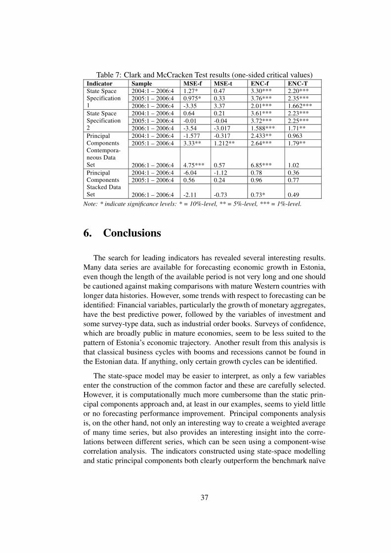
Table 7: Clark and McCracken Test results (one-sided critical values)Indicator Sample MSE-f MSE-t ENC-f ENC-T
2004:1 – 2006:4 1.27* 0.47 3.30*** 2.20***
2005:1 – 2006:4 0.975* 0.33 3.76*** 2.35***
State Space
Specification
1 2006:1 – 2006:4 -3.35 3.37 2.01*** 1.662***
2004:1 – 2006:4 0.64 0.21 3.61*** 2.23***
2005:1 – 2006:4 -0.01 -0.04 3.72*** 2.25***
State Space
Specification
2 2006:1 – 2006:4 -3.54 -3.017 1.588*** 1.71**
2004:1 – 2006:4 -1.577 -0.317 2.433** 0.963
2005:1 – 2006:4 3.33** 1.212** 2.64*** 1.79**
Principal
Components
Contempora-
neous Data
Set 2006:1 – 2006:4 4.75*** 0.57 6.85*** 1.02
2004:1 – 2006:4 -6.04 -1.12 0.78 0.36
2005:1 – 2006:4 0.56 0.24 0.96 0.77
Principal Components
Stacked Data
Set 2006:1 – 2006:4 -2.11 -0.73 0.73* 0.49
Note: * indicate significance levels: * = 10%-level, ** = 5%-level, *** = 1%-level.
6. Conclusions
The search for leading indicators has revealed several interesting results.
Many data series are available for forecasting economic growth in Estonia,
even though the length of the available period is not very long and one should
be cautioned against making comparisons with mature Western countries with
longer data histories. However, some trends with respect to forecasting can be
identified: Financial variables, particularly the growth of monetary aggregates,
have the best predictive power, followed by the variables of investment and
some survey-type data, such as industrial order books. Surveys of confidence,
which are broadly public in mature economies, seem to be less suited to the
pattern of Estonia’s economic trajectory. Another result from this analysis is
that classical business cycles with booms and recessions cannot be found in
the Estonian data. If anything, only certain growth cycles can be identified.
The state-space model may be easier to interpret, as only a few variables
enter the construction of the common factor and these are carefully selected.
However, it is computationally much more cumbersome than the static prin-
cipal components approach and, at least in our examples, seems to yield little
or no forecasting performance improvement. Principal components analysis
is, on the other hand, not only an interesting way to create a weighted average
of many time series, but also provides an interesting insight into the corre-
lations between different series, which can be seen using a component-wise
correlation analysis. The indicators constructed using state-space modelling
and static principal components both clearly outperform the benchmark naïve
37

AR(1) model in in-sample testing. However, this seems to be due to a very
strong performance in the earlier part of the sample, particularly during the
Russian crisis. The performance in the latter part of the sample, particularly
in 2006, seems to be rather poor, which is confirmed by out-of-sample testing.
This might be due to a systemic change; that is, factors other than the financial
variables we identified might have taken over the driving of economic devel-
opment in Estonia. However, this could also be a temporary break.
38

References
Altissimo, F., Bassanetti, A., Cristadoro, R., Forni, M., Hallin, M., Lippi, M.
and Reichlin, L., 2001. EuroCOIN: a real time coincident indicator of the euro
area business cycle. CEPR Working Paper 3108.
Artis, M., Banerjee, A. and Marcellino, M., 2001. Factor Forecasts for the
UK. EUI Working Paper No. 2001/15.
Bai, J. and Ng, S., 2002. Determining the number of factors in approximate
factor models. Econometrica 70:191–221.
Bandholz, H., 2004. Konjunkturelle Frühindikatoren für die Bundesrepublik
Deutschland und die Freie und Hansestadt Hamburg. Frankfurt am Main: Pe-
ter Lang.
Bandholz, H. and Funke, M., 2003. In Search of Leading Indicators of Eco-
nomic Activity in Germany. Journal of Forecasting 22:277–297.
Breitung, J. and Eickmeier, S., 2005. Dynamic factor models. Deutsche Bun-
desbank Discussion Paper.
Bry, G. and Boschan, C., 1971. Cyclical Analysis of Time Series: Selected
Procedures and Computer Programs. In National Bureau of Economic Re-
search. New York.
CESIfo, 2007. World Economic Survey. Vol. 6. CESIfo, No. 4.
Chen, S.-S., 2005. A Note on In-Sample and Out-of-Sample Tests for Granger
Causality. Journal of Forecasting, No. 24:453–464.
Clark, T. E. and McCracken, M. W., 2001. Tests of Forecast Accuracy and
Encompassing for Nested Models. Journal of Econometrics, No. 105:85–110.
Curran, D. and Funke, M., 2006. Taking the temperature — forecasting GDP
growth for mainland China. BOFIT Discussion Papers, No. 6.
D’Agostino, A. and Giannone, D., 2006. Comparing alternative predictors
based on large-panel factor models. ECB Working Paper Series.
Diebold, F. X. and Mariano, R. S., 1995. Comparing predictive accuracy.
Journal of Business Economic Statistics, No. 13:253–263.
Dreger, C. and Schuhmacher, C., 2004. Estimating Large-Scale Factor Models
for Economic Activity in Germany: Do They Outperform Simpler Models?
Jahrbücher für Nationalökonomie und Statistik, No. 224:731–750.
39

Eickmeier, S. and Breitung, J., 2005. How synchronized are Central and East
European economies with the euro area? Evidence from a structural factor
model. Bundesbank Discussion Paper Series 1: Economic Studies.
Estrella, A. and Mishkin, F. S., 1998. Predicting U.S. Recessions: Financial
Variables as Leading Indicators. The Review of Economics and Statistics, No.
80:45–61.
Forni, M., Hallin, M. and Lippi, M., 2003. The Generalized Dynamic Factor
Model one-sided estimation and forecasting. Journal of the American Statisti-
cal Association.
Forni, M., Hallin, M., Lippi, M. and Reichlin, L., 2001. Coincident and lead-
ing indicators for the Euro area. The Economic Journal.
Forni, M., Lippi, M. and Reichlin, L., 2000. The Generalized Factor Model:
Identification and Estimation. The Review of Economics and Statistics, No.
82:540–554.
Fritsche, U. and Stephan, S., 2000. Leading Indicators of German Busi-
ness Cycles: an Assessment of Properties. Deutsches Institut für Wirtschafts-
forschung (DIW), Berlin.
G. C. o. E. E. (Sachverständigenrat),(2005). Annual Report 2003/2004.
Gerlach, S. and Yiu, M. S., 2005. A dynamic factor model of economic activ-
ity in Hong Kong. Pacific Economic Review, No. 10:279–292.
Granger, C. W. J. and Newbold, P., 1977. Forecasting Economic Time Series.
Orlando: Academic Press.
Harvey, D. I., Leybourne, S. J. and Newbold, P., 1998. Tests for Forecast
Encompassing. Journal of Business Economic Statistics, No. 16:254–259.
Jolliffe, I. T., 2002. Principal Component Analysis. New York: Springer.
Kalman, R. E., 1960. A New Approach to Linear Filtering and Prediction
Problems. Journal of Basic Engineering, Transactions of the ASME, Series D.
Kalman, R. E., 1963. New Methods in Wiener Filtering Theory. In Proceed-
ings of the First Symposium of Engineering Applications of Random Function
Theory and Probability. (Eds, Bogdanoff, J. L. and Kozin, F.). New York: Wi-
ley, 270–388.
40

Kapetanios, G. and Marcellino, M., 2006. Impulse Response Functions from
Structural Dynamic Factor Models: A Monte Carlo Evaluation. CEPR Dis-
cussion Paper, No. 5621.
Kim, C.-J., 1999. State-space models with regime switching: classical and
Gibbs-sampling approaches with applications. Cambridge, Mass.: MIT Press.
Marcellino, M., Stock, J. H. and Watson, M. W., 2000. A dynamic factor
analysis of EMU.
McCracken, M. W., 1999. Asymptotics for out-of-sample tests of causality.
Louisiana State University.
Nerb, G., 2007. The Importance of Representative Surveys of Enterprises for
Empirically Oriented Business Cycle Research. In Handbook of Survey-Based
Business Cycle Analysis (Ed, Goldrian, G.). Cheltenham: Edward Elgar.
Stock, J. H. and Watson, M. W., 1991. A Probability Model of the Coincident
Economic Indicators. In Leading Indicators: New Approaches and Forecast-
ing Records (Eds, Lahiri, K. and Moore, G. H.). Cambridge, UK: Cambridge
University Press, 63–89.
Stock, J. H. and Watson, M. W., 2002. Forecasting Using Principal Compo-
nents from a Large Panel of Predictors. Journal of the American Statistical
Association, No. 97:147–162.
Zanghieri, P., 2006. Current account dynamics in the new Member States. In
The Central and Eastern European Countries and the European Union (Eds,
Artis, M., Banerjee, A. and Marcellino, M.). Cambridge: Cambridge Univer-
sity Press, 245–273.
41

Appendix 1. Data set and cross correlations
No. Name of Series Transformation ADF
(p-value)
Max
X-corr
at lag
(-lead)
1
Assets with BIS-reporting
banks
YOY change 0.00 0.16 0
2 Brazilian Stock Market Index YOY change 0.01 0.45 2
3 Chinese Stock Market Index YOY change 0.22 -0.26 -4
4
Commercial banks' foreign
assets
YOY change 0.00 0.31 2
5
Commercial banks' foreign
liabilities
YOY change 0.33 0.24 1
6
Construction building activity
over the past 3 months
YOY change 0.00 0.43 1
7
Construction confidence
indicator
YOY change 0.00 0.46 -1
8
Construction employment over
the next 3 months
YOY change 0.01 0.39 1
9
Construction factors limiting
building activity ** insufficient
demand
YOY change 0.01 -0.44 1
10
Construction factors limiting
building activity ** weather
conditions
YOY change 0.00 0.33 2
11 Construction order books YOY change 0.17 0.50 -1
12
Construction prices over the
next 3 months
YOY change 0.18 0.53 0
13 Consumer confidence Indicator YOY change 0.11 0.55 0
14
Consumer financial situation of
households over next 12
months
YOY change 0.01 0.34 -1
15
Consumer financial situation of
households over past 12 months
YOY change 0.00 0.31 -3
16
Consumer major purchases over
next 12 months
YOY change 0.01 0.33 -1
17
Consumer perception of change
in unemployment
YOY change 0.11 -0.58 0
18
Consumer perception of general
economic situation over next 12
months
YOY change 0.01 0.38 1
19
Consumer perception of general
economic situation over past 12
months
YOY change 0.00 0.52 1
20 Consumer price index (av) YOY change 0.01 -0.26 3
21
Consumer price Index at end of
period
YOY change 0.00 -0.21 0
22 Current Account share of GDP
Levels, de-
seasonalised
0.00 -0.52 -2
23 Current-Account balance YOY change 0.00 0.33 1
24 Deposit interest rate YOY change 0.00 0.68 -2
25 Economic sentiment indicator YOY change 0.20 0.60 0
26 Estonian interest rate spread YOY change 0.00 0.28 0
27 Euro zone real GDP YOY change 0.05 -0.35 4
29 FDI as share of GDP Levels 0.00 0.27 -3
30 Finnish exports YOY change 0.38 -0.22 4
42

No. Name of Series Transformation ADF
(p-value)
Max
X-corr
at lag
(-lead)
31 Finnish imports YOY change 0.14 0.15 2
32 Finnish Real GDP YOY change 0.00 -0.31 4
33
Foreign direct investment
Change yoy
YOY change 0.00 0.25 2
34 Foreign-exchange reserves YOY change 0.05 0.30 -2
35 Estonian Real GDP change YOY change 0.06 1.00 0
36 Gold, national valuation YOY change 0.87 0.29 1
37 Industrial confidence indicator YOY change 0.03 0.58 1
38
Industrial current export
order books
YOY change 0.00 0.54 1
39
Industrial current overall
order books
YOY change 0.00 0.60 1
40
Industrial current stock
of finished products
YOY change 0.00 -0.46 0
41 Industrial production index YOY change 0.00 0.84 0
42
Industrial production over
the past 3 months
YOY change 0.02 0.49 2
43
Industrial production will over
the next 3 months
YOY change 0.00 0.27 1
44
Industrial selling prices will
over the next 3 months
YOY change 0.01 0.39 4
45 International reserves YOY change 0.05 0.30 -2
46 Lending interest rate (%) YOY change 0.00 0.67 -3
47
Liabilities with BIS-reporting
banks
YOY change 0.37 0.41 -1
48
Loan Stock granted to
commercial undertakings
YOY real change 0.40 0.51 0
49
Loan Stock granted to
individuals
YOY real change 0.14 0.58 1
50 Money market interest rate (%) YOY change 0.11 0.49 -1
51 Net taxes on products YOY change 0.02 0.80 0
52 New Car Registrations YOY change 0.02 0.56 0
53
Real effective exchange rate of
the kroon
YOY change 0.01 -0.60 0
54 Retail Confidence indicator YOY change 0.00 0.47 1
55
Retail Employment over
the next 3 months
YOY change 0.00 0.52 0
56
Retail orders placed with
suppliers during the next 3
months
YOY change 0.00 0.47 0
57 Retail Stocks YOY change 0.00 0.30 -3
58 Russian GDP YOY real change 0.01 0.35 0
59 Stock of money M1 YOY real change 0.02 0.71 1
60 Stock of money M2 YOY real change 0.01 0.68 0
43

No. Name of Series Transformation ADF
(p-value)
Max
X-corr
at lag
(-lead)
61 Tallinn Stock Market Index YOY real change 0.06 0.54 1
62 Total exports fob Change yoy YOY change 0.04 0.36 0
63 Total imports cif Change yoy YOY change 0.02 0.34 0
64 Trade balance (fob-cif basis) YOY change 0.08 0.15 1
65
Value Added in Agriculture,
Hunting
YOY real change 0.00 0.37 0
66 Value Added in Construction YOY real change 0.00 0.64 -1
67 Value Added in Education YOY real change 0.00 -0.25 3
68
Value Added in Electricity, Gas
and Water Supply
YOY real change 0.00 0.36 0
69
Value Added in Financial
Intermediation
YOY real change 0.17 0.55 1
70 Value Added in Fishing YOY real change 0.03 0.41 0
71 Value Added in Forestry YOY real change 0.07 -0.25 3
72
Value Added in Health and
Social Work
YOY real change 0.00 -0.25 1
73
Value Added in Hotels,
Restaurants
YOY real change 0.00 0.39 0
74 Value Added in Manufacturing YOY real change 0.02 0.83 0
75
Value Added in Mining,
Quarrying
YOY real change 0.02 0.65 0
76
Value Added in Other
community, social and personal
service activities
YOY real change 0.01 0.49 0
77
Value added in Public
Administration and Defence;
compulsory social security
YOY real change 0.01 -0.34 4
78
Value Added in Real Estate,
Renting and Business Activities
YOY real change 0.00 0.56 0
79
Value Added in Transport,
Storage, Communication
YOY real change 0.00 0.41 0
80
Value Added in Wholesale and
Retail Trade
YOY real change 0.00 0.39 -1
44

Appendix 2. Principal components: time series in-
cluded
No. Series Name Short name Type
1 Interest rate spread (long-term
minus short-term) est_intrsprd_yoygr Finance
2 Effective exchange rate Exch_periodave_yoygr Finance
3 Brazilian stock exchange cbrazil_s Finance
4 Current account as share of
GDP CA_SHARE Finance
5 Chinese stock exchange CCHINA Finance
6 Loans to Commercial
Customers CREDIT_COM_RYOYGR Finance
7 Loans to Individuals CREDIT_IND_RYOYGR Finance
8 Real Money Supply M1 M1REAL_YOYGR Finance
9 Real Money Supply M2 M2REAL_YOYGR Finance
10 Foreign Direct Investment (%
of GDP) FDI_share Finance
11 Tallinn stock exchange TALLINN_SI_LINKED_YOYGR Finance
12 Value added in Education va_educ_yoygr Sector
13 Value added in retail and wholesale trade va_reta_yoygr Sector
14 Value added in
Transportation, etc. va_tran_yoygr Sector
15 Value added in Financial
Intermediation va_bank_yoygr Sector
16 Construction Prices over next
three months ct_prices_com3m Survey
17 Households’ financial situation over next twelve
months cs_hh_fin_com12m Survey
18 Households’ expectations of the state of the economy over
next twelve months cs_economy_com12m Survey
19 Households’ financial
situation over last twelve
months cs_hh_fin_past12m Survey
20 Consumer confidence cs_confidence Survey
21 Manufacturing Prices over next twelve months in_price_com3m Survey
22 Retail trade confidence re_confidence Survey
23 Industrial production over last
three months in_prod_past3m Survey
24 Consumers’ perception of the state of the economy over last
twelve months cs_economy_past12m Survey
25 Industrial order books, exports in_orderbooks_exp Survey
26 Industrial confidence in_confidence Survey
27 Industrial order books, overall in_orderbooks Survey
28 Russian real GDP rgdp_rus_yoygr Trade
29 Euro zone real GDP rgdp_euro_yoygr Trade
30 Finnish real GDP rgdp_fin_yoygr Trade
31 New car sales NEW_CAR_SALES_EST_YOYGR Trade
45

Eesti Pank Bank of Estonia
Working Paper Series
2/2008
Forecasting Economic Activity
for Estonia: The Application of
Dynamic Principal Components
Analysis
Christian Schulz

The Working Paper is available on the Eesti Pank web site at:
www.bankofestonia.info/pub/en/dokumendid/publikatsioonid/seeriad/uuringud/
For information about subscription call: +372 6680 998; Fax: +372 6680 954
e-mail: [email protected]
ISBN 978-9949-404-68-1
ISSN 1406-7161

Forecasting Economic Activity for Estonia:
The Application of Dynamic Principal
Components Analysis
Christian Schulz
Abstract
In this paper, the dynamic common factors method of Forni et al.
(2000) is applied to a large panel of economic time series on the Es-
tonian economy. In order to improve forecasting of economic activity in
Estonia, we derive a leading indicator composed of the common com-
ponents of twelve series, which were identified as leading. The resulting
indicator performs better than two other indicators, which are based on
a small-scale state-space model used by Stock and Watson (1991) and a
large-scale static principal components model used by Stock and Watson
(2002), respectively. It also clearly outperforms the naïve benchmark in
both in-sample and out-of-sample forecast comparisons.
JEL Code: C32, C33, C53, E37
Keywords: Estonia, forecasting, turning points, dynamic factor models, dy-
namic principal components, forecast performance
Author’s e-mail address: [email protected]
The views expressed are those of the author and do not necessarily represent
the official views of Eesti Pank.

Non-technical summary
The Estonian economy, like most economies of the Central and Eastern
European Countries (CEEC) is growing at a very fast pace. However, many
observers are worried about the strong foreign currency inflows and high cur-
rent account deficits, particularly in Estonia (IMF World..., 2007:89–92). As
the strong economic growth and the business opportunities associated with
this are reasons for these inflows, particularly foreign direct investment, con-
siderable attention is being directed at good short-term forecasts of economic
activity in Estonia. National institutions (central bank, ministries), interna-
tional institutions (e. g. EU, IMF) and the local and international financial
communities rely on continuously improving forecasting methods.
In this paper, we apply a method developed by Forni, Hallin, Lippi and
Reichlin (FHLR, 2000), to derive a short-term leading indicator for economic
activity in Estonia. The advantages of this method include:
• The method allows the efficient use of large panels of economic time
series: there are many economic time series available for Estonia; how-
ever, compared to the data available for most Western countries, the
length of the time series is rather short. The use of large panels there-
fore increases the total information available.
• The method allows the derivation of one or few common factors which
can be used for forecasting: the information contained in the large panel
of data is condensed into only one leading indicator based on the "com-
mon" components of the time series, i. e. cleaned of their ididosyncratic
components.
• The method allows the discrimation between series as leading or lagging
with respect to economic activity at relevant frequencies: dynamic prin-
cipal components methodology allows us to look at measures of coher-
ence at relevant cycle lengths. Other methodologies like static principal
components are prone to the overemphasis on very short-term correla-
tions.
We find that indeed, the derived leading indicator, which is a combination
of the common components of twelve leading time series, outperforms alter-
native forecasting models. Both in-sample testing according to Diebold and
Mariano (1995) and pseudo out-of-sample testing according to Clark and Mc-
Cracken (2001) indicate clear improvements over models based on small-scale
state-space models (Stock and Watson, 1991) and large scale static principal
components based models (Stock and Watson, 2002).
2

In this paper, we pay additional attention to a correct specification of growth
cycles in Estonia. We find that a particularly good way to do this is the use
of a three-state Markov switching model, similar to the one used by Hamil-
ton (1989). Estonia has been in a true recession (by Western standards) only
once in the aftermath of the Russian crisis in the late 1990s. Before and af-
ter, however, growth has been shifting between periods of sustainable growth
(particularly for the five years following the Russian crisis) and periods of
booming and probably unsustainable growth just before the Russian crisis and
since 2005. This endogenous cycle dating method seems to yield better re-
sults than the popular Bry and Boschan (1971) cycle dating method used by
the American National Bureau of Economic Research (NBER).
3

Contents
1. Introduction . . . . . . . . . . . . . . . . . . . . . . . . . . . . . . 5
2. Literature review . . . . . . . . . . . . . . . . . . . . . . . . . . . 6
3. Empirical framework . . . . . . . . . . . . . . . . . . . . . . . . . 8
4. The Estonian Data Set . . . . . . . . . . . . . . . . . . . . . . . . . 9
5. Forecasting Economic Growth for Estonia . . . . . . . . . . . . . . 19
6. Conclusions . . . . . . . . . . . . . . . . . . . . . . . . . . . . . . 25
References . . . . . . . . . . . . . . . . . . . . . . . . . . . . . . . . . 27
Appendix 1. Data Set and Sources and Cross-correlation with Respect
to the Reference Series . . . . . . . . . . . . . . . . . . . . . . . . 31
4

1. Introduction
The Baltic countries have been enjoying an economic boom for many years
now and are rapidly catching up with Western European countries on a num-
ber of important indices of economic development; for instance, output per
capita. According to Walter et al. (2006), Estonia will have overtaken Por-
tugal in terms of GDP per capita in purchasing-power parity equivalents by
2020, while Lithuania will not be far behind. However, there have repeatedly
been concerns and warnings that at least the pace of this catch-up process is
not sustainable at its current levels. For example, Fitch, the rating agency,
warned Latvia in March 2007 of the downgrading of its debt if it does not
get its rampant current-account deficit of about 20% under control.1 It is of-
ten said that the mix of rapidly rising property prices and the inflexible cur-
rency board exchange rate regimes fuels the presumably unsustainable booms
in these countries.2 On the other hand, some studies take a more positive
stance on this topic, as particularly in Estonia, much of the current account
deficit is financed by foreign direct investment.3 In any case, because of the
relatively high inflation rates, the adoption of the single currency will not occur
in the short-term, so the countries’ central banks will have to remain vigilant
with regard to output and price developments. In this paper, we will take a
look at the data from Estonia and try to figure out which elements really drive
Estonian economic activity. The aim is to develop reliable short-term lead-
ing indicators for economic activity in order to improve the tools available for
macroeconomic analysis.
When we forecast economic activity, large panels of macroeconomic data
are usually available. Intuitively, it is attractive to use the information revealed
in as much of this data as possible in order to perform forecasts. This is es-
pecially true when trying to forecast activity in Eastern European countries,
where the length of the available data series is short and the frequency often
low, so that the number of observations is small. There are several techniques
that allow us to combine information from large panels of data, mainly with
the aim of reducing the dimensionality of the data set to a small number of
unobservable series which contain a very large proportion of the information.
Two competing approaches in the current literature are static principal com-
ponents, which were used by Stock and Watson (2002), and many others; and
1The Economist, March 10th 2007:54.2All three Baltic countries operate currency-board-type exchange rate regimes with ex-
change rates fixed to the Euro, thereby effectively abandoning independent monetary policies.
Estonia introduced a peg to the Deutsche Mark in 1992, Lithuania to the Euro in 2002 and
Latvia to the Euro in 2005. Latvia had pegged its currency to the SDR-basket, which is dom-
inated by the US Dollar.3See Walter et al. (2006).
5

dynamic principal components, used by Forni et al. (2000). Having applied
static principal components to an Estonian data set with mixed results, our
aim in this paper is to add to the existing forecasting literature by applying
dynamic principal components analysis.4 We will start by briefly outlining the
model used, estimate the common components and use this step to investigate
relationships between the variables and the reference series, which will be real
economic growth, specifically with respect to their leading characteristics. We
will then proceed to combine the common components identified via dynamic
principal components methodology in the frequency domain, and apply the re-
sulting composite leading index to a forecasting model. Before concluding, we
will compare the results to different alternative indicators and forecast speci-
fications.5 We use in-sample and out-of-sample testing procedures to conduct
these tests.
2. Literature review
The application of dynamic principal components to the estimation of com-
mon factors and macroeconomic analysis was principally developed by Forni
et al. (2000) and applied in numerous papers, first by the same authors in
Forni et al. (2001) to a Euro zone data set. Many papers deal with economic
forecasting, mainly for economic growth and inflation in countries or groups
of countries. Forni et al. (2001) apply this methodology to the construction of
coincident and leading indicators for the Euro Area, for instance, while Artis
et al. (2001) do so for the United Kingdom. It is this methodology that we
will be using in this paper. Static principal components were introduced to
economic forecasting by Stock and Watson (2002), who apply their method to
US data.
Several papers compare the results of the two methodologies; for instance
D’Agostino and Giannone (2006), who compare dynamic and static principal
component forecasts for the US economy and conclude that neither method
outperforms the other. Similar results are achieved by Boivin and Ng (2005),
and Schumacher (2005). Forni et al. (2003b) compare dynamic principal
components to structural VARs, finding that although the forecasting appli-
cations of dynamic principal components have been successful, identification
and, particularly, economic interpretation are difficult. They go on to attempt
to overcome this.
Forni et al. (2003a) note that the original dynamic principal components
methodology may not be suitable for forecasts as it is based on a two-sided
4See Schulz (2007).5See Schulz (2007).
6

filter and is therefore weak at the two ends of the sample. Consequently, they
enhance the method to a two-step procedure, which makes it a one-sided es-
timation and forecast. They find that the resulting forecasts outperform Stock
and Watson’s (2002) static principal components-based forecasts for the same
US data set. Kapetanios and Marcellino (2006) add impulse-response func-
tions as a tool for analysing structural models based on dynamic principal
components analysis.6
There is another branch of the literature based on dynamic principal com-
ponents which does not deal with economic forecasting. Much of it is based
on the fact that the frequency domain can also be used for measures of co-
hesion; that is, synchronisation, as proposed by Croux et al. (2001), where a
measure of cohesion is used to analyse business cycle synchronisation. Eick-
meier and Breitung (2005) use dynamic principal components to analyse the
level of synchronisation between EMU countries and EU accession countries,
and within these respective groups of countries. Forni et al. (2007) use dy-
namic principal components to identify and estimate structural shocks to an
economy, where they show that their model is superior to VAR models when
very large cross-sections of data are being used.
Besides these papers, which deal with the estimation of common factors
by principal components-type models, there are some papers that develop ad-
ditional techniques, such as the optimal choice of the number of factors to be
included in the forecasting model (Bai and Ng, 2002). Another field is the de-
velopment of in-sample and out-of-sample forecast performance testing meth-
ods; for example, in Diebold and Mariano (1995) or Clark and McCracken
(2001). An additional tool occasionally referred to in this literature is the use
of business cycle dating methods like the one developed by Bry and Boschan
(1971), which is an essential foundation for the frequency domain literature,
where standard definitions of typical business cycle lengths are relevant to the
estimation techniques. We will make use of some of these techniques, partic-
ularly in testing, where suitable.
In addition to the principal-components-related literature, there is also a
section of literature on small-scale state-space-type common factor models,
building on work by Stock and Watson (1991). More recently, this branch
of the literature has focused on state-dependent analysis, particularly Markov
switching as introduced by Hamilton (1989). These models using a single
factor have been applied to the US by Kim and Nelson (1999) and Chauvet
(1998), and to Germany by Bandholz and Funke (2003); or the use of two
factors for Europe by Kholodolin and Yao (2005). These techniques will not
be explicitly referred to in this paper.
6Kapetanios and Marcellino (2006) use the Stock and Watson (2002a) data set for the US.
7

3. Empirical framework
In this paper, we will apply dynamic principal components analysis, an
approach developed by Forni, Hallin, Lippi and Reichlin (2000). We start by
decomposing a data set xt into two unobservable components:7
xt = γqt + ξq
t (1)
The data set is assumed to be stationary and zero-mean; that is, the data
set has to be pre-transformed accordingly. The residual vector ξqt represents
the idiosyncratic components of the data set after the common component has
been subtracted. The term γqt = (γq
1t...γqnt) contains the common part of the
series and reflects the linear projection of xt on the space generated by unob-
servable q common factors zt.
zht = ph (L) xt, h = 1, ..., q (2)
These common factors are a linear combination of the leads and lags of xt,
so L is the lag operator and ph(L) is a (1 × n) row vector of two-sided linear
filters. Any two common factors are mutually orthogonal and the filters are
normalised so that ph(L)pk(L− 1)′ = 0 when h 6= k and 1 otherwise. We can
therefore expand (1) as follows:
xt = γqt + ξq
t = Cq(L)zqt + ξq
t = Kq(L)xt + ξqt (3)
If the filters ph(L) and the common component processes zt maximise the
explained variance∑n
j=1 var(γqjt), then they can be called the “dynamic prin-
cipal components” of xt. They are very similar to the static principal compo-
nents used for instance in Stock and Watson (2002) in the sense that they are
related to the eigenvalues and eigenvectors of a matrix. However, instead of
the variance-covariance matrix, the spectral density matrix of xt,∑
(ω) is used
here where −π < ω < π is the frequency at which the spectral density matrix
is evaluated. The filter vector ph(e−iω) is the eigenvector associated with the
h-th eigenvalue of the spectral density matrix, after sorting these eigenvalues
in descending order.
As with the static case, the filters Cq(L) and Kq(L) can be expressed ex-
plicitly as follows:
7More details on the methodology can be found in Forni at al. (2000). The software
we implemented was the BUSY software (http://eemc.jrc.ec.europa.eu/softwareBUSY.htm)
developed by Fiorentini and Planas (2003). Following the notation in Forni et al. (2000),
vectors and matrices are printed in bold letters, with scalar variables in italics.
8

Cq(L) =(
p1(L−1)′ . . . pq(L
−1)′)
(4)
Kq(L) = Cq(L)Cq(L−1)′ = p1(L−1)′p1(L) + . . . + pq(L
−1)′pq(L) (5)
Kq(L) is first estimated in the frequency domain as
Kq(ω) = p1(ω)′p1(ω) + . . . + pq(ω)′pq(ω) (6)
This matrix must be evaluated over a finite number of frequencies, a pro-
cedure described in Forni et al. (2000) by first estimating the spectral density
matrix∑
(ω) at each frequency and then using the eigenvalues and eigen-
vectors of each spectral density matrix to compute Kq(e−iθ). Kq(L) is then
estimated using the inverse Fourier transform of Kq(e−iθ).8 Kq(L) can now be
used as the filter to derive the common components:
γqt = Kq(L)xt (7)
Therefore, we can decompose each series into a common part and an idio-
syncratic part:
xt = γqt + ξ∗t (8)
In the following sections, we will make use of these common parts for two
purposes. First, they may be used to classify the series as leading or lagging
with respect to a reference series. Secondly, they can be used in forecasting.
4. The Estonian Data Set
The data set for Estonia includes 76 economic time series.9 All the series
are of quarterly frequency and are available from the first quarter of 1994 until
8For a thorough treatment of frequency domain time series analysis, in particular dynamic
principal components, spectral density matrices, fourier transforms and power spectra, consult
Brillinger (1981).9This number is in line with other studies that use similar data panels and estimation
techniques for business cycle analysis or forecasting exercises; e. g., Eickmeier and Breitung
(2005) use 235 series (but only a maximum of 41 different ones for each country), Kapetanios
and Marcellino (2006) use 148 series for the US, and Forni et al. (2007) use 89 series, again
for the US. A Study on Eastern Europe by Banerjee et al. uses between 40 and 60 quarterly
series for each country from 1994:1 until 2002:4 (2006). These authors are not using the same
methodology in their papers, however.
9

the fourth quarter of 2006. Like other authors (Banerjee et al., 2006), we
find that monthly series are not always available for the whole time period in
Central and Eastern Europe. The data set includes (see Appendix 1):
• Financial data: monetary aggregates, loan aggregates, price indices, in-
terest rates, and monetary reserves. In addition, stock market indices for
the Tallinn stock exchange, as well as an American (S&P 500), a Euro
zone (EuroStoxx 50) and an Emerging Markets (BRIC) stock exchange
index are included;
• Survey-type data: European Commission surveys of industry, consumers,
construction, service and retail on various aspects such as order books,
economic expectations, and perceptions of the current economic situa-
tion and the recent past;
• Trade-related data: data on principal trading partners (Euro zone, Fin-
land, Russia), as well as Estonian imports and exports;
• Sectoral data: data on the various sectors of the Estonian economy in
value-added terms.
All series have been converted to year-on-year growth rates. This avoids
more complicated techniques for de-seasonalisation and achieves stationarity
in all the series. Several other techniques for de-seasonalisation and stationar-
ity are available, among them in particular Baxter-King-type band-pass filters
and the Hodrick-Prescott filter. While these techniques are interesting for busi-
ness cycle analysis, their results are more difficult to interpret for forecasting
exercises.10
If we want to predict the economic situation in Estonia, we first have to
look at its growth pattern over a period we can consider (see Figure 1). To
avoid the early transition pains encountered by Estonia as it struggled to shake
off Soviet influence, we start in the first quarter of 1995. Another reason for
beginning at this point is that the data before is only partially available and of
sometimes questionable quality. At this time, we use the GDP time series as
they were published before 2006. In 2006, major changes were made in the
collection and calculation methodologies as part of the harmonisation process
with EU standards. This update changed GDP levels by up to 6.0%, according
to the 2006 Annual Report by Statistics Estonia, and growth figures, which are
more relevant to this paper, changed somewhat as well. Unfortunately, only
10Another implication for forecasting is that because of the rather short time series avail-
able, only short-term forecasts of one quarter ahead should be performed (Banerjee et al.,
2006).
10

data from 2000 onwards is currently available under the new methodology.
This time span is too short for the methodologies we employ later on. There-
fore, until the longer time series under the new methodology are ready and
published by the Statistics Office of Estonia later this year, we must link the
old data with the new.
-.04
.00
.04
.08
.12
.16
1996 1998 2000 2002 2004 2006
GDP_EST_YOYGR_LINKED
Figure 1: Real GDP Growth in Estonia (% yoy, constant 2000 prices)
Year-on-year-growth (from –4% up to +16%) is presented on the y-axis,
and it can be seen that since 2000, growth has fluctuated, but has been positive
throughout. Before, there was a brief phase of strong growth running up until
1998, followed by a sharp decline in growth and even a brief period of negative
growth. It can also be seen that growth has significantly exceeded the corridor
between 5% and 9% since 2005.
We employ two techniques in order to obtain a feeling for the cyclicality of
economic growth in Estonia. Firstly, we use the Markov switching method as
a descriptive statistic of phases, similarly to Hamilton (1989); and secondly,
the NBER dating algorithm, further on below. Markov switching allows us to
model the time series of growth rates, where the average growth rate depends
upon the state the economy is in; for example, “expansion” or “recession”,
which are treated as “probabilistic objects”.11 Certain parameters (only the
mean growth rate in our case) are assumed to follow a state-dependent data
11Diebold and Rudebusch (1996).
11

generation process.12 In other words, the state is assumed to be endogenous
rather than pre-determined, and there is a probability ps at each point t for the
economy being in state st. Therefore, we start by fitting the following AR(2)
switching model to the series of seasonally adjusted13 quarterly growth rates:
gdpqt − µs = φ1(gdpq
t−1 − µst−1) + φ2(gdpq
t−2 − µst−2) (9)
The state-variable st takes on the values 1, 2 and 3 and is assumed to follow
a first-order latent three-state Markov chain process with transition probability
matrix M, where p12 = prob(st = 2 |st−1 = 1) etc. The rows of M add up to
1.
M =
p11 p12 p13
p12 p22 p23
p13 p23 p33
(10)
We deviate from Hamilton (1989), who only used two states, because a
brief glance at the Estonian data shows that, except for the recession phase
in the late nineties, growth is almost always high. Yet there might be dif-
ferences in this high-growth pattern which could not be detected if only two
states are allowed for.14 The resulting conditional probabilities for being in
the respective states are depicted in the Figure 2.15 We display both filtered
and smoothed probabilities. The former probabilities take into account infor-
mation available up to the point of estimation, while the latter use information
from the whole sample for smoothing.16
12Other authors allow more parameters that depend on states, such as the variance-
covariance matrix (Lahiri and Wang, 1994).13Seasonal adjustment is performed using the Census X12 method. We will continue to
use the four-quarter growth rates later on, but in this analysis it makes more sense to use
quarter-on-quarter growth rates to avoid persistence and derive clear cycle-lengths.14Business cycles as defined classically in Burns and Mitchell (1946) are not identifiable in
Estonia; “growth cycles” would be a more correct characterisation. This implies the two states
of “expansion” and “contraction” mentioned before and applied in most of the relevant liter-
ature for mature economies (see Diebold and Rudebusch (1996) or Lahiri and Wang (1994)).
There are papers that introduce more than two states as well (Emery and Koenig, 1992).15We use the Ox-MSVAR-package.16The filtered probabilities are P (st = i |xt) and the smoothed probabilities are P (st =
i |xT ) , where xt is the series of quarterly real GDP growth.
12

Pro
bab
ility
of b
ein
g in
sta
te
0%
20
%
40
%
60
%
80
%
10
0%
19
95
:01 1
99
5:0
3 19
96
:01 1
99
6:0
3 19
97
:01 1
99
7:0
3 19
98
:01 1
99
8:0
3 19
99
:01 1
99
9:0
3 20
00
:01 2
00
0:0
3 20
01
:01 2
00
1:0
3 20
02
:01 2
00
2:0
3 20
03
:01 2
00
3:0
3 20
04
:01 2
00
4:0
3 20
05
:01 2
00
5:0
3 20
06
:01 2
00
6:0
3
0%
20
%
40
%
60
%
80
%
10
0%
19
95
:01 1
99
5:0
3 19
96
:01 1
99
6:0
3 19
97
:01 1
99
7:0
3 19
98
:01 1
99
8:0
3 19
99
:01 1
99
9:0
3 20
00
:01 2
00
0:0
3 20
01
:01 2
00
1:0
3 20
02
:01 2
00
2:0
3 20
03
:01 2
00
3:0
3 20
04
:01 2
00
4:0
3 20
05
:01 2
00
5:0
3 20
06
:01 2
00
6:0
3
1 (
Recessio
n)
1= -
0.0
4 %
2 (
Su
sta
inable
Gro
wth
)
2= 0
.86
%
3 (
Bo
om
)
3= 1
.61
%
19
95
:11
99
6:1
199
7:1
19
98
:11
999
:1200
0:1
20
01:1
2002
:1200
3:1
20
04:1
2005
:12
00
6:1
0%
20
%
40
%
60
%
80
%
10
0%
19
95
:01 1
99
5:0
3 19
96
:01 1
99
6:0
3 19
97
:01 1
99
7:0
3 19
98
:01 1
99
8:0
3 19
99
:01 1
99
9:0
3 20
00
:01 2
00
0:0
3 20
01
:01 2
00
1:0
3 20
02
:01 2
00
2:0
3 20
03
:01 2
00
3:0
3 20
04
:01 2
00
4:0
3 20
05
:01 2
00
5:0
3 20
06
:01 2
00
6:0
3
-1%
-1%
0%
1%
1%
2%
2%
3%
Sea
son
ally
Adju
ste
d Q
uart
erl
y
Gro
wth
Rate
Sm
oo
thed
Proba
bilitie
sFilte
red P
robab
ilities
Fig
ure
2:
Mar
kov
-Sw
itch
ing
Sta
teP
rob
abil
itie
sfo
rse
aso
nal
lyad
just
edq
uar
ter-
on
-qu
arte
rg
row
thra
tes
13

The first state indicates a recession and can only be found in the late nineties
– during the Russian crisis. State 3, which had an average annualised growth
rate of 6.6%, occurs significantly twice, once just before the Russian crisis
and again towards the end of the sample.17 As the transition probability p33 –
that a boom quarter is followed by another boom quarter – is 0.67, the average
duration of a boom is 1/(1− p33) ≈ 3 quarters, so this latest boom should end
very soon if the pattern is to repeat itself. The average annualised growth rate
in state 2, dubbed “Sustainable Growth”, is 3.5% and its average duration is
5 to 6 quarters. Notice that states 2 and 3 are not necessarily business cycles
in the classical sense, but rather “growth cycles”, the use of which for further
analysis seems more practical given the pattern of continually high growth in
Estonia. We will go on and compare the results to the NBER analysis.
To obtain another formalised view of potential business cycle turning points,
a method developed by Bry and Boschan (1971) for dating business cycles
is often used and referred to as the American National Bureau of Economic
Research (NBER) method. Here, we adapt it to the identification of growth-
cycles; that is, cycles in the quarterly year-on-year growth rates of GDP. The
Figure 3 displays the results.
-.04
.00
.04
.08
.12
.16
1996 1998 2000 2002 2004 2006
GDP_EST_YOYGR_LINKED
Figure 3: Growth Cycles of the Estonian Economy
17We attribute significance here when the conditional probability of one state exceeds 0.9,
according to Neftci (1984). Alternatively, some papers suggest 0.5 as the critical value (Band-
holz and Funke, 2003).
14

There are four growth-cycle recessions that can be identified using Bry
and Boschan’s method: 1996:1–1996:4, 1997:2–1999:2, 2001:2–2002:2, and
2006:1–. The last downturn in particular seems to contradict the results of the
Markov switching analysis. However, upon close visual inspection, one might
observe that the probability of being in state 3 – a “boom” – peaks at 2006:1
and then drops. This hints at a turning point to a less buoyant economic phase.
Next we analyse the measures of the co-movement of the data in the data set
with respect to the reference series, which is real GDP growth in Estonia. This
can be performed both in the time domain using cross-correlations at different
leads and lags and in the frequency domain using measures of coherence, such
as the one proposed by Croux et al. (2001). The cross-correlation of the
reference series xrgdp with series i at lead/lag k is defined as:
ρrgdp,i(k) =Cov(xrgdp,t, xi,t−k)
√
V ar(xrgdp,t)V ar(xi,t)), for i = 1, . . . , N (11)
(Squared) coherence of the reference series xrgdp with series j at frequency
ω is defined as the squared modulus of the cross-spectra divided by the product
of the spectra of the reference series and of the j-th series:
Coh(ω)2 =|frgdp,j(ω)|2
frgdp,rgdp(ω)fjj(ω)
, for j = 1, . . . , N (12)
In other words, it is a continuum across the frequency band [−π, π] and not
one number, as with the cross-correlation. In this definition, f are the spectra
and cross-spectra of the series in the data set, given by
frgdp,j(ω) =1
sπ
∞∑
k=−∞
ρrgdp,j(k)e−iωk (13)
We use the Bartlett spectral window instead of all the cross-covariances
ρrgdp,j .18 The results for both cross-correlation and coherence analysis are
displayed in the following table. We use averages over the periodicities of
1–2 years and 2–8 years for coherence in order to avoid lengthy displays of
coherence graphs. In addition to the descriptive statistics explained above, we
show the transformations performed (none) and the frequency of the data input
(all quarterly), as well as another descriptive statistic, the mean delay, which
measures the lag in the movements of the series with respect to the reference
series (see Table 1; the full names and sources of the series can be found in
Appendix 1).19
18See Fuller (1996) for reference.19The cross-spectrum between the reference series and another series j, which is generally
complex, can be written in polar coordinates as frgdp,j(ω) = |frgdp,j(ω)|w−iPh(ω). Then
15

Table 1: Behaviour of the Data Set with Respect to the Reference Series
CHARACTERISTICS COHEREN CE M EAN DELA Y CROSS-CORRELATION
SERIES
Transf. Freq. 2 Y-8 Y 1 Y-2 Y 2 Y-8 Y 1 Y-2 Y r0 rm ax tma x(1)
BRIC_yoygr X 4 0,03 0,07 1,23 0,90 0,12 0,49 2
CA_SHARE X 4 0,26 0,15 7,31 2,64 -0,32 -0,62 -2
CA_yoygr X 4 0,08 0,06 0,32 0,41 0,17 0,31 1
CPI_yoygr X 4 0,06 0,06 -7,30 -2,65 -0,25 -0,31 3
CREDIT_COM_RYOYGR X 4 0,30 0,27 -0,02 -0,03 0,50 0,50 0
CREDIT_IND_RYOYGR X 4 0,31 0,30 0,17 0,17 0,51 0,59 1
cs_confidence X 4 0,40 0,34 0,04 0,05 0,54 0,55 1
cs_economy_com12m X 4 0,20 0,15 0,13 0,15 0,34 0,43 1
cs_economy_past12m X 4 0,35 0,31 0,11 0,11 0,51 0,55 1
cs_hh_fin_com12m X 4 0,15 0,10 -0,06 -0,05 0,28 0,38 -2
cs_hh_fin_past12m X 4 0,12 0,09 -0,01 0,02 0,26 0,41 -3
cs_purc_com12m X 4 0,23 0,15 -0,03 -0,01 0,32 0,38 1
cs_unemployment X 4 0,51 0,45 -7,43 -2,77 -0,63 -0,63 0
ct_activity_past3m X 4 0,12 0,12 0,45 0,43 0,26 0,42 1
ct_confidence X 4 0,25 0,21 -0,01 -0,02 0,42 0,44 -1
ct_employment_com3 m X 4 0,18 0,15 0,12 0,12 0,35 -0,44 -4
ct_lf_demand X 4 0,25 0,17 -7,43 1,29 -0,37 -0,46 2
ct_lf_weather X 4 0,01 0,02 -3,60 -1,29 0,04 0,32 -2
ct_orderbooks X 4 0,26 0,21 -0,06 -0,08 0,41 0,47 -1
ct_prices_com3m X 4 0,33 0,31 0,06 0,06 0,52 0,52 0
econ_sentiment_yoygr X 4 0,52 0,44 -0,04 -0,05 0,60 0,62 -1
est_intrsprd_yoygr X 4 0,11 0,09 0,08 0,06 0,27 0,39 4
eustoxx_yoygr X 4 0,00 0,01 0,21 0,15 0,08 -0,29 -4
Exch_periodave_yoygr X 4 0,38 0,38 -7,34 -2,69 -0,59 -0,59 0
exports_f in_yoygr X 4 0,02 0,01 -0,10 -0,07 0,11 -0,21 4
exports_yoygr X 4 0,17 0,15 -0,07 -0,08 0,36 0,37 -1
FDI_share X 4 0,00 0,00 7,17 2,57 -0,05 0,23 -3
FDI_yoygr X 4 0,02 0,01 0,07 0,07 0,11 0,26 -4
Fin_assets_yoygr X 4 0,01 0,00 -7,17 -2,51 -0,05 -0,13 4
fin_cbass_yoygr X 4 0,03 0,01 -0,07 -0,09 0,07 0,30 -2
fin_cblia_yoygr X 4 0,01 0,01 0,30 0,37 0,07 -0,20 4
Fin_liab_yoygr X 4 0,09 0,11 -0,30 -0,28 0,30 -0,40 4
forexreserve_yoygr X 4 0,09 0,08 -0,16 -0,14 0,26 0,35 -4
gold_yoygr X 4 0,19 0,17 0,05 0,06 0,39 0,40 1
imports_fin_yoygr X 4 0,03 0,02 0,01 0,02 0,15 0,28 -3
Imports_yoygr X 4 0,16 0,14 -0,05 -0,04 0,36 0,36 0
ind_prod_yoygr X 4 0,64 0,63 0,06 0,05 0,77 0,77 0
intreserves_yoygr X 4 0,09 0,08 -0,16 -0,14 0,27 0,35 -4
Intr_depo_yoygr X 4 0,23 0,26 -0,49 -0,46 0,42 0,73 -2
Intr_lend_yoygr X 4 0,03 0,08 -1,67 -1,05 0,10 0,71 -3
in_confidence X 4 0,34 0,32 0,26 0,25 0,51 0,59 1
in_orderbooks X 4 0,30 0,32 0,35 0,32 0,50 0,61 1
in_orderbooks_exp X 4 0,27 0,30 0,30 0,27 0,50 -0,60 -4
in_pr ice_com3m X 4 0,11 0,11 0,31 0,31 0,28 0,38 3
in_production_com3m X 4 0,08 0,06 0,17 0,21 0,19 0,28 1
in_prod_past3m X 4 0,10 0,14 0,74 0,61 0,26 -0,51 -4
in_stock X 4 0,34 0,28 -7,28 -2,62 -0,49 -0,50 1
M1REAL_YOY GR X 4 0,46 0,45 0,25 0,25 0,62 0,74 1
M2real_yoygr X 4 0,52 0,50 0,14 0,14 0,67 0,69 1
price_cons_yoygr X 4 0,05 0,05 -7,36 -2,70 -0,24 -0,26 3
re_confidence X 4 0,24 0,22 0,28 0,27 0,39 0,49 1
the mean delay is defined as the phase at frequency ω divided by that frequency or Ph(ω)/ω.
For further reference, see Harvey (1990).
16

CHARACTERISTICS COHERENCE MEAN DELAY CROSS-CORRELATION
SERIES
Transf. Freq. 2 Y-8 Y 1 Y-2 Y 2 Y-8 Y 1 Y-2 Y r0 rm ax tmax(1)
re_emplo_com3m X 4 0,45 0,36 -0,01 -0,02 0,54 0,54 0
re_order_supply_com3m X 4 0,35 0,27 0,02 0,00 0,45 0,45 0
re_stocks X 4 0,08 0,05 -7,26 -2,59 -0,15 -0,29 4
rgdp_euro_yoygr X 4 0,00 0,00 7,38 2,73 -0,04 -0,45 4
rgdp_fin_yoygr X 4 0,03 0,03 -0,24 -0,26 0,14 -0,39 4
rgdp_rus_yoygr X 4 0,12 0,12 0,13 0,12 0,34 0,41 3
taxes_yoygr X 4 0,75 0,70 0,02 0,01 0,80 0,80 0
Trade_bal_yoygr X 4 0,03 0,03 0,03 0,07 0,17 0,17 0
us_snp500_yoygr X 4 0,02 0,02 7,40 2,73 -0,12 -0,30 4
Va_agri_yoygr X 4 0,12 0,10 -0,19 -0,17 0,29 0,29 0
va_bank_yoygr X 4 0,37 0,31 0,27 0,27 0,46 0,55 1
va_cons_yoygr X 4 0,42 0,40 -0,20 -0,20 0,58 0,63 -1
va_educ_yoygr X 4 0,02 0,01 7,36 2,54 -0,08 -0,34 4
va_elec_yoygr X 4 0,20 0,17 -0,14 -0,15 0,39 0,39 0
va_fish_yoygr X 4 0,15 0,15 -0,07 -0,06 0,38 0,38 0
va_heal_yoygr X 4 0,07 0,05 -7,35 -2,69 -0,18 -0,21 1
va_hosp_yoygr X 4 0,14 0,15 -0,16 -0,16 0,38 0,38 0
va_manu_yoygr X 4 0,71 0,69 0,05 0,05 0,80 0,80 0
va_mini_yoygr X 4 0,45 0,42 0,09 0,09 0,62 0,62 0
va_publ_yoygr X 4 0,08 0,06 7,33 2,62 -0,22 -0,39 4
va_real_yoygr X 4 0,41 0,38 0,10 0,11 0,59 0,59 0
va_reta_yoygr X 4 0,17 0,11 -0,17 -0,24 0,26 0,40 -1
va_soci_yoygr X 4 0,26 0,24 0,12 0,12 0,47 0,47 0
va_tran_yoygr X 4 0,20 0,19 -0,11 -0,10 0,40 0,40 0
Note: The +/(–) sign refers to a lead(lag) with respect to the reference series; Transformation X signals no further
transformation
Given that we are looking for short-term leading indicators from a rather
small sample, we shall consider only series with high cross-correlations at
small lags (1 or 2) when we look at time domain cross-correlations. As in
our previous paper, we find that financial data such as monetary aggregates or
credit growth show particularly promising features. In addition, some survey-
type series are leading, as well as the financial services series from the sectoral
data. Trade-related data seems less promising.
Moving on to the frequency domain, we have to consider both coherence
and the mean delay to identify the possibility of a useful leading series.20 The
estimation parameters were set as follows: as a smoothing type, we have used
the Bartlett window as mentioned above. Another often discussed parameter
is the number of dynamic common factors to be estimated. Here we include
as many factors as we need to explain at least 50% of the variance in the data
sample, a threshold used by other authors such as Eickmeier and Breitung
20Altissimo et al. (1999) propose considering cross-coherences of 0.4 or higher and con-
sider mean delays of more than one period (>1.0) as useful leading series.
17

(2005), and Forni et al. (2003a).21 In the estimation of the spectra, we include
three cross-correlations for each series. We discuss the results of this specified
estimation in the following section.
The classification of the series’ leading or lagging behaviour with respect to
the reference series can be performed using their common components’ spec-
tral density matrix∑q∗
γ (ω), or more specifically, the mean delay (see above)
in its first row. This yields the results described in Table 2.
Table 2: Classification Results for the Time Series in the Data Set
PHASE OPPOSITION LEADING SERIES COINCIDENT SERIES LAGGING SERIES
CA_SHARE BRIC_yoygr CA_yoygr in_orderbooks CA_SHARE
CPI_yoygr CPI_yoygr CREDIT_COM_RYOYGR in_orderbooks_exp ct_lf_demand
cs_unemployment cs_unemployment CREDIT_IND_RYOYGR in_price_com3m FDI_share
ct_lf_demand ct_lf_weather cs_confidence in_production_com3m FDI_yoygr
ct_lf_weather Exch_periodave_yoygr cs_economy_com12m M1REAL_YOYGR fin_cbass_yoygr
Exch_periodave_yoygr Fin_assets_yoygr cs_economy_past12m M2real_yoygr Fin_liab_yoygr
Fin_assets_yoygr in_prod_past3m cs_hh_fin_com12m re_confidence Intr_depo_yoygr
in_stock in_stock cs_hh_fin_past12m re_emplo_com3m Intr_lend_yoygr
price_cons_yoygr price_cons_yoygr cs_purc_com12m re_order_supply_com3m Us_snp500_yoygr
re_stocks re_stocks ct_activity_past3m rgdp_euro_yoygr va_heal_yoygr
rgdp_euro_yoygr va_educ_yoygr ct_confidence rgdp_fin_yoygr
va_educ_yoygr va_publ_yoygr ct_employment_com3m rgdp_rus_yoygr
va_heal_yoygr ct_orderbooks taxes_yoygr
va_publ_yoygr ct_prices_com3m Trade_bal_yoygr
econ_sentiment_yoygr Va_agri_yoygr
est_intrsprd_yoygr va_bank_yoygr
Eustoxx_yoygr va_cons_yoygr
exports_fin_yoygr va_elec_yoygr
exports_yoygr va_fish_yoygr
fin_cblia_yoygr va_hosp_yoygr
forexreserve_yoygr va_manu_yoygr
gold_yoygr va_mini_yoygr
imports_fin_yoygr va_real_yoygr
Imports_yoygr va_reta_yoygr
ind_prod_yoygr va_soci_yoygr
intreserves_yoygr va_tran_yoygr
in_confidence
The results differ dramatically from those before. Besides the method-
ological difference, this also has to do with the strict application of the cri-
terion that the mean delay has to be larger than 1 period/quarter to make a
series a leading one.22 Interestingly, surveys like the assessment of stocks
21Other papers either use informal criteria to choose the number of factors (Stock and
Watson, 2002a) or a formal criterion (Bai and Ng, 2002), where the results lead to a similar
amount of explained variance.22Accordingly, series where the mean delay is between 1 and –1 are considered as contem-
poraneous and series with a mean delay smaller than –1 are considered as lagging.
18

by retail businesses and industrial firms, which are both in phase opposition
to the reference series, are among the leading series. The consumer price
index is also on the list, as well as the effective exchange rate. In fact, all
series, except for the BRIC stock index, are in phase opposition to the refer-
ence series.23 A comparison with the classification in other studies (for ex-
ample, Forni et al. (2001)), yields some resemblances. For instance, interest
rates (intr_depo_yoygr and intr_lend_yoygr) can be found among the lag-
ging variables. By contrast, we do not find industrial order book variables
(in_orderbooks and in_orderbooks_exp) among the leading variables. How-
ever, Forni et al. (2001) define variables as already leading when they have a
mean delay of 0.33 quarters – one month – where we define a lead of more
than one quarter as the threshold.
5. Forecasting Economic Growth for Estonia
There are obviously many ways to make use of the information contained
in the estimated common components. Forni et al. (2001) suggest simply tak-
ing a weighted average of the series classified as leading according to the mean
delays of their common components. In the following, we suggest using the
common components directly. This is implicitly done by most papers that use
static principal components, such as Stock and Watson (2002) or Banerjee et
al. (2006), who use one or more static principal components of their respective
entire data sets for forecasting, or this author, who uses only series previously
identified as leading and combines them by applying static principal compo-
nents. Our leading indicator will be defined as follows:
Λq =1
m
m∑
j=1
γqj − γq
j
σγq
j
, for j = 1, . . . , N (14)
This is the equally weighted aggregate of the standardised common com-
ponents of the m leading series. Series which were in phase opposition are
multiplied by –1. It is important to notice that the estimate of the common
components is poor at the ends of the sample as the filter Kq(L) is a two-sided
filter with the length 2M + 1, where M = 3 in our specification — for the
last four and the first four periods there are no direct estimates of the com-
mon components. However, we replace these missing values using the linear
projections of each common component on the present (forecasting) and past
23In the Appendix 1, we supply the time domain analysis of the common components. The
short-term cross-correlations of the common components with respect to the reference series
are displayed.
19

(backcasting) of the average of all the coincident variables and on the average
of the leading variables.24 The Figure 4 depicts the resulting leading indicator
and the reference series, real GDP growth in Estonia.
-16
-12
-8
-4
0
4
8
12
-.08
-.04
.00
.04
.08
.12
.16
.20
1996 1998 2000 2002 2004 2006
COMPOSITE_LEADING GDP_EST_YOYGR_LINKED
Figure 4: Reference Series and Indicator – Comparison and Turning Points
Note: Triangles denote turning points identified using the NBER dating method.
It can be seen that the leading indicator is in phase with the reference series
— a rise indicates increasing growth in economic activity and a fall indicates
decreasing growth in economic activity. As a crude measure of performance,
we analysed the turning points in the original reference series and in the indi-
cator series applying the NBER dating method, which is based on the method
developed by Bry and Boschan (1971), adjusted for quarterly series.25 It can
be seen that the turning points in the first half of the sample are reliably pre-
dicted within a few quarters. Later, the trough in the reference series in 2003:1
is predicted 7 quarters ahead of its occurrence, which is too long a delay to
be considered valuable information. The last peak in the reference series is
missed by one quarter. However, the indicator series is much clearer than the
24Alternatively, we could have followed the much more complicated use of one-sided fil-
tered covariance matrices of the common and idiosyncratic components of the variables pro-
posed by Forni et al. (2003a).25Some authors argue that the prediction of turning points is more important than number
forecasts, at least in some circumstances, and particularly with policy makers (Chin et al.,
2000).
20

reference series, which declines slightly and slowly after this peak. The in-
dicator series shows that Estonia is clearly in a phase of declining economic
growth after 2005.
As a plausibility check, we also construct the composite coincident and
lagging indicators. To this end we combine the common components of the
series in the data set, which were identified as coincident and lagging, respec-
tively, according to formula (14).26 The resulting cross-correlations profile of
the three indicators with respect to the reference series (real GDP growth) is
depicted in the Figure 5.
-0,6
-0,4
-0,2
0
0,2
0,4
0,6
0,8
1
1,2
10 9 8 7 6 5 4 3 2 1 0 -1 -2 -3 -4 -5 -6 -7 -8 -9 -10
Lag ( -Lead)
Cross-Correlation
Coincident Ind ica tor
Lagg ing Indic ator
Lead ing Indicator
Figure 5: Phase-shifts between leading, coincident and lagging indicators
It can be seen that the dynamic principal components methodology has sep-
arated the series very well. The combined common components of the coinci-
dent series, for instance, achieve a coincident (lead/lag 0) cross-correlation of
more than 0.9. The lagging indicator’s cross-correlation profile peaks at lead
2 and the leading indicators at lag 2.
Following most of the literature on dynamic principal components, we
compare the performance in number forecasting in comparison with alterna-
tive indicators and forecasting models. Here, we compare our new composite
indicator with indicators we developed in our previous paper.27 This paper
suggested the following four indicators:
26See Table 2.27Schulz (2007).
21

1. A state-space model using the industrial orderbooks assessment, mon-
etary aggregate M1 and commercial loans based on methods used in
Stock and Watson (1991) (iInd3S).
2. Another state-space model using the industrial orderbooks assessment,
monetary aggregate M1 and the Tallinn Stock exchange based on the
same method (iio_m1_tsi).
3. A static principal components model based on 31 time series identified
as leading by cross-correlation analysis based on the methods used in
Stock and Watson (2002a) (“contemporaneous data set”)(PCCont).
4. A static principal components model based on the 31 time series identi-
fied as leading and their respective first lags based on the same method
(“stacked data set”)(PCStack).
First, we will use the same in-sample testing routine developed by Diebold
and Mariano (1995) to compare the indicators. The procedure regresses the
difference between the absolute forecast errors of two series on a constant,
using robust standard errors and checks the t-value of the constant.28
Overall, we compare six specifications, of which the naïve AR(1) model of
real GDP growth (15) will serve as the benchmark model. Note that we use
static fitted forecasts. This means that each quarter, the actual value of GDP
growth is multiplied by the fitted regression coefficients rather than using a
fitted value of GDP growth. This is done for all specifications pair-wise with
the benchmark model, which is defined as follows:
gdpt = cnaive + b1,naive · gdpt−1 + enaive (15)
The forecasting model for our composite dynamic principal components
leading indicator is defined as follows:
gdpt = cdyn + b1,dyn · gdpt−1 + b2,dyn · Λqt−1 + edyn (16)
The state-space models are very similar, only the composite leading indi-
cator is replaced by the respective leading indicators derived by state-space
modelling.
28Much of the dynamic principal components literature only uses the root-mean-squared
forecasting error in order to compare different forecasts (D’Agostino and Giannone, 2006),
which reveals whether differences between forecasts are significant. Other papers (Curran
and Funke, 2006) use more sophisticated techniques; for instance, the procedures developed
by Clark and McCracken (2001).
22

gdpt = cind3S + b1,ind3S · gdpt−1 + b2,ind3S · iind3S,t−1 + eind3S (17)
gdpt = cio_m1_tsi + b1,io_m1_tsi · gdpt−1 (18)
+b2,io_m1_tsi · iio_m1_tsi,t−1 + eio_m1_tsi
Notice that we are dealing with a nested testing procedure, where only
the first lag of the composite is added to the model in the first three models.
For the two static principal components-based models, we use the first three
components so the forecasting specifications appear as follows:
gdpt = cPC,Cont + b1,PC1,Cont · gdpt−1 + b2,PC1,Cont · PC1,Cont,t−1 (19)
+b3,PC2,Cont · PC2,Cont,t−1 + b4,PC3,Cont · PC3,Cont,t−1 + ePC,Cont
gdpt = cPC,Stack + b1,PC1,Stack · gdpt−1 + b2,PC1,Stack · PC1,Stack,t−1 (20)
+b3,PC2,Stack · PC2,Stack,t−1 + b4,PC3,Stack · PC3,Stack,t−1 + ePC,Stack
We calculate the p-values for the t-test on the constant; that is, a small p-
value indicates that the alternative performs better than the benchmark. The
Table 3 reports the p-values for different specifications and periods.
The results look very promising: as the only constructed indicator, our
new composite leading indicator outperforms the benchmark model in every
evaluation period, in many cases significantly so. Particularly important is
the impressive performance in 2006, where all the other indicators performed
badly. In many other periods, for instance 1999 or 2002, it is not far from
the best forecasting model. We conclude that our new indicator presents a
significant improvement over the other models.
Second, we use out-of-sample testing because many papers, including Cur-
ran and Funke (2006), D’Agostino and Giannone (2006), and Artis et al.
(2001) suggest out-of-sample performance testing as a better tool for evalu-
ation (see Table 4).29 In out-of-sample testing, the forecasting model is es-
timated for a sub-sample of the entire available sample and then forecasts
29However, this is not done in all papers. Many only use in-sample testing; for instance,
Bandholz and Funke (2003).
23

Table 3: Forecasting Performance of Alternative Models and Model Specifi-
cations
Period State Space Specification 1
State Space Specification 2
Principal Components
Contemporaneous Data Set
Principal Components
Stacked Data Set
Dynamic Principal Components Data
Set
1996Q1 – 1996Q4 x x 0.75 0.54 0.01***
1997Q1 – 1997Q4 x x 0.10* 0.09* 0.28
1998Q1 – 1998Q4 0.00*** 0.00*** 0.03** 0.25 0.00***
1999Q1 – 1999Q4 0.20 0.11 0.11 0.06* 0.16
2000Q1 – 2000Q4 0.08 0.11 0.27 0.27 0.36
2001Q1 – 2001Q4 0.32 0.19 0.00*** 0.22 0.00***
2002Q1 – 2002Q4 0.46 0.37 0.09 0.11 0.25
2003Q1 – 2003Q4 0.34 0.23 0.01*** 0.06 0.06*
2004Q1 – 2004Q4 0.31 0.25 0.46 0.27 0.49
2005Q1 – 2005Q4 0.19 0.08* 0.34 0.29 0.30
2006Q1 – 2006Q4 0.98 0.46 0.61 0.90 0.02**
1996Q1 – 2006Q4 x x 0.01*** 0.02** 0.01***
1998Q1 – 2006Q4 0.01*** 0.00*** 0.02** 0.04** 0.01***
2004Q1 – 2006Q4 0.34 0.11 0.38 0.23 0.18
2005Q1 – 2006Q4 0.51 0.11 0.36 0.32 0.10*
RMSFE 0.02 0.02 0.02 0.02 0.02
Note: The lowest/best p-value for each evaluation period is printed in bold letters.
Table 4: Clark and McCracken Test results (one-sided critical values)
Indicator Sample MSE-f MSE-t ENC-f ENC-T
2004:1 – 2006:4 1.27* 0.47 3.30*** 2.20***
2005:1 – 2006:4 0.975* 0.33 3.76*** 2.35***
(16) State Space Specification 1
2006:1 – 2006:4 -3.35 3.37 2.01*** 1.662***
2004:1 – 2006:4 0.64 0.21 3.61*** 2.23***
2005:1 – 2006:4 -0.01 -0.04 3.72*** 2.25***
(17) State Space Specification 2
2006:1 – 2006:4 -3.54 -3.017 1.588*** 1.71**
2004:1 – 2006:4 -1.577 -0.317 2.433** 0.963
2005:1 – 2006:4 3.33** 1.212** 2.64*** 1.79**
(18) Principal Comp. Contemporaneous Data Set 2006:1 – 2006:4 4.75*** 0.57 6.85*** 1.02
2004:1 – 2006:4 -6.04 -1.12 0.78 0.36
2005:1 – 2006:4 0.56 0.24 0.96 0.77
(19) Principal Components Stacked Data Set 2006:1 – 2006:4 -2.11 -0.73 0.73* 0.49
2004:1 – 2006:4 3.68*** 2.32*** 2.63*** 3.11***
2005:1 – 2006:4 2.87*** 2.36*** 1.90*** 2.85***
(20) Dynamic Principal Components 2006:1 – 2006:4 2.18*** 1.98*** 1.58*** 2.70***
Note: * indicates significance levels: * = 10%-level, ** = 5%-level, *** = 1%-level.
24

for the remaining sample are evaluated with respect to the actual values. We
perform the test procedures used by Clark and McCracken (2001) using the
same nested forecasting model specifications as in (15) through (20), with
(15) again serving as the benchmark model. Four different statistics are sug-
gested by Clark and McCracken: the two MSE (mean squared error) statistics
test for equal forecasting accuracy. The MSE-t test was proposed by Granger
and Newbold (1977), while critical values for the MSE-f test were provided by
McCracken (1999). The ENC (encompassing) statistics test for the benchmark
model encompasses the alternative. The ENC-T test is described in Clark and
McCracken (2001) and draws from Diebold and Mariano (1995), and Harvey
et al. (1998). The ENC-f test was developed by Clark and McCracken (2001)
and uses variance weighting to improve the small-sample performance of the
encompassing test.
The results clearly show that the composite leading indicator based on dy-
namic principal components performs better in out-of-sample forecasting than
the competing forecasting models. All tests for all selected periods show sig-
nificance, indicating that the model outperforms the benchmark naïve model.
The results are very encouraging as both in-sample and out-of-sample show
a significant improvement in forecasting performance over all the competing
models.
6. Conclusions
Economic forecasting for Eastern European economies is a challenging
task as the available indicators have a short history and have been influenced
by possibly singular events like the breakdown of the Soviet-dominated trad-
ing block and the emerging markets’ crisis in the late 90s. As the length of the
available time series is short, the present paper uses larger cross-sections of
data to accumulate extra information. This idea has been partly exploited by
other papers on Eastern European states, particularly by Banerjee et al. (2006).
To our knowledge, this is the first study to undertake this task using dynamic
principal components for Estonia.
We have successfully employed the dynamic principal components method-
ology to develop a short-term leading indicator for the Estonian economy. We
used the common components of the data set identified using dynamic prin-
cipal components analysis in the frequency domain to classify a sub-set of
series as leading and using the common components of these series to con-
struct a composite leading indicator. The results of the classification are quite
different from the results in our earlier paper in the time domain, with variables
from a variety of backgrounds (surveys, price indices, sectoral data) forming
25

the group of leading variables.30 However, the resulting indicator, which we
constructed by simple aggregation, does seem to perform better than indicators
developed using different methods, according to in-sample and out-of-sample
testing. These other methods include state-space modelling as in Stock and
Watson (1991) as well as static principal components as in Stock and Wat-
son (2002a). It performs particularly well in 2006, the end of the estimation
sample, where other indicators were shown to be rather deficient compared
to simple autoregressive forecasts. We believe that this methodology should
be used in regular forecasting exercises as it reveals a lot of extra information
about the behaviour of the many series with respect to the reference series.
The methodology also presents a more sophisticated way of performing the
classification of series in leading, contemporaneous and lagging series with
respect to the reference series than the classic cross-correlation analysis.31
30Schulz (2007).31Using cross-correlations to analyse the leading and lagging characteristics of variables
with respect to each other is standard in the empirical literature – for instance, see Bandholz
and Funke (2003), and Forni et al. (2001). Gerlach and Yiu (2005) use contemporaneous
correlations and principal components to pre-identify variables useful for the construction of
a common factor of economic activity in Hong Kong.
26

References
Altissimo, F., Marchetti, D., Oneto, G. P., 1999. New Coincident and Leading
Indicators for the Italian Economy. Bank of Italy. Mimeo.
Artis, M., Banerjee, A., Marcellino, M., 2001. Factor Forecasts for the UK.
EUI Working Paper, No. 15.
Bai, J., Ng, S., 2002. Determining the Number of Factors in Approximate
Factor Models. Econometrica, No. 70:191–221.
Bandholz, H., Funke, M., 2003. In Search of Leading Indicators of Economic
Activity in Germany. Journal of Forecasting, No. 22:277–297.
Banerjee, A., Marcellino, M., Masten, I., 2006. Forecasting Macroeconomic
Variables for the New Member States. In The Central and Eastern European
Countries and the European Union (Eds, Artis, M., Banerjee, A. and Mar-
cellino, M.). Cambridge: Cambridge University Press.
Boivin, J., Ng, S., 2005. Understanding and Comparing Factor-Based Fore-
casts. Mimeo.
Brillinger, D. R., 1981. Time Series Data Analysis and Theory. New York:
Holt, Rinehart and Winston.
Bry, G., Boschan, C., 1971. Cyclical Analysis of Time Series: Selected Pro-
cedures and Computer Programs. In National Bureau of Economic Research.
New York.
Burns, A. F., Mitchell, W. C., 1946. Measuring Business Cycles. New York:
National Bureau of Economic Research.
Chauvet, M., 1998. An Econometric Characterization of Business Cycle Dy-
namics with Factor Structure and Regime Switching. International Economic
Review, No. 39:969–996.
Chin, D., Geweke, J., Miller, P., 2000. Predicting Turning Points. Technical
Paper Series Congressional Budget Office.
Clark, T. E., McCracken, M. W., 2001. Tests of Forecast Accuracy and En-
compassing for Nested Models. Journal of Econometrics, No. 105:85–110.
Croux, C. M., Forni, M., Reichlin, L., 2001. A Measure for Co-movement for
Economic Variables: Theory and Empirics. The Review of Economics and
Statistics, No. 83:231–241.
27

Curran, D., Funke, M., 2006. Taking the Temperature — Forecasting GDP
Growth for Mainland China. BOFIT Discussion Papers, No. 6.
D’Agostino, A., Giannone, D., 2006. Comparing Alternative Predictors Based
on Large-Panel Factor Models. ECB Working Paper Series.
Diebold, F. X., Mariano, R. S., 1995. Comparing Predictive Accuracy. Journal
of Business & Economic Statistics, No. 13:253–263.
Diebold, F. X., Rudebusch, G. D., 1996. Measuring Business Cycles: A Mod-
ern Perspective. Review of Economics and Statistics, No. 78:67–77.
Eickmeier, S., Breitung, J., 2005. How Synchronized are Central and East
European Economies with the Euro Area? Evidence from a Structural Factor
Model. Bundesbank Discussion Paper Series 1: Economic Studies.
Emery, K. M., Koenig, E. F., 1992. Forecasting Turning Points: Is a Two-
State Characterization of Business Cycles Appropriate? Economics Letters,
No. 39:431–435.
Fiorentini, G., Planas, C., 2003. Busy Programme: Tools and Practices for
Business Cycle Analysis in the European Union.
Forni, M., Giannone, D., Lippi, M., Reichlin, L., 2007. Opening the Black
Box – Structural Factor Models with Large Cross-Sections. European Central
Bank Working Paper Series.
Forni, M., Hallin, M., Lippi, M., 2003a. The Generalized Dynamic Factor
Model: One-Sided Estimation and Forecasting. Journal of the American Sta-
tistical Association forthcoming.
Forni, M., Hallin, M., Lippi, M., Reichlin, L., 2001. Coincident and Leading
Indicators for the Euro Area. The Economic Journal.
Forni, M., Lippi, M., Reichlin, L., 2000. The Generalized Factor Model:
Identification and Estimation. The Review of Economics and Statistics, No.
82:540–554.
Forni, M., Lippi, M., Reichlin, L., 2003b. Opening the Black Box: Structural
Factor Models Versus Structural VARs. CEPR Discussion Paper.
Fuller, W. A., 1996. Introduction to Statistical Time Series. New York: John
Wiley&Sons.
Gerlach, S., Yiu, M. S., 2005. A Dynamic Factor Model of Economic Activity
in Hong Kong. Pacific Economic Review, No. 10:279–292.
28

Granger, C. W. J., Newbold, P., 1977. Forecasting Economic Time Series.
Orlando: Academic Press.
Hamilton, J. D., 1989. A New Approach to the Economic Analysis of Nonsta-
tionary Time Series and the Business Cycle. Econometrica, No. 57:357–384.
Harvey, A., 1990. The Econometric Analysis of Time Series. Cambridge,
Mass., MIT Press.
Harvey, D. I., Leybourne, S. J., Newbold, P., 1998. Tests for Forecast Encom-
passing. Journal of Business & Economic Statistics, No. 16:254–259.
Kapetanios, G., Marcellino, M., 2006. Impulse Response Functions from
Structural Dynamic Factor Models: A Monte Carlo Evaluation. CEPR Dis-
cussion Paper, No. 5621.
Kholodilin, K. A., Yao, K. W., 2005. Measuring and Predicting Turning Points
Using a Dynamic Bi-Factor Model. International Journal of Forecasting, No.
21:525–537.
Kim, C.-J., Nelson, C. R., 1999. State-space Models with Regime Switching:
Classical and Gibbs-Sampling Approaches with Applications. Cambridge,
Mass., MIT Press.
Lahiri, K., Wang, J. G., 1994. Predicting Cyclical Turning Points with Leading
Index in a Markov Switching Model. Journal of Forecasting, No. 13:245–263.
McCracken, M. W., 1999. Asymptotics for Out-of-Sample Tests of Causality.
Louisiana State University.
Neftci, S., 1984. Are Economic Time Series Asymmetric Over the Business
Cycle? Journal of Political Economy, No. 92:307–328.
Schulz, C. H., 2007. Forecasting Economic Growth for Estonia: Application
of Common Factor Methodologies. Bank of Estonia Working Paper Series.
Schumacher, C., 2005. Forecasting German GDP Using Alternative Factor
Models Based on Large Data Sets. Deutsche Bundesbank Discussion Paper,
No. 24.
Stock, J. H., Watson, M. W., 1991. A Probability Model of the Coincident
Economic indicators. In Leading Indicators: New Approaches and Forecast-
ing Records (Eds, Lahiri, K. and Moore, G. H.). Cambridge, UK: Cambridge
University Press.
29

Stock, J. H., Watson, M. W., 2002. Forecasting Using Principal Components
from a Large Number of Predictors. Journal of the American Statistical Asso-
ciation, No. 97:147–162.
Stock, J. H., Watson, M. W., 2002a. Macroeconomic Forecasting Using Dif-
fusion Indexes. Journal of Business & Economic Statistics, No. 20:147–162.
Walter, N., Becker, W., Mühlberger, M., 2006. Estonia, Lithuania, Slovenia:
Poised to adopt the Euro. In Deutsche Bank Research EU-Monitor.
30

Appendix 1. Data Set and Sources and Cross-correlation
with Respect to the Reference Series
Data Set and Sources
Shortname NAME TYPE SOURCE DEFINITION
BRIC_yoygr Emerging Markets Stock Index (Brazil, Russia, India, China)
Finance IFC, Monthly Review of Emerging Stock Markets; Quar terly Re vie w of
Emerging Stock Markets
Composite stock market index (29/12/1983=100) in local currency; year-on-year-change as
unweighted avera ge of four stock exchanges
CA_SHARE Current Account share
of GDP seasonally adjusted
Trade Eesti Pank SA X12 census
CA_yoygr Current-a cc ount balance
Trade IMF, International Financial Statistics
Trade balance, plus net services, plus net income, plus net current
transfers. Line 78ald in the IFS.
CPI_yoygr Consumer pric e Index
end of period
Finance Statistical Office of
Estonia, Eesti Pank
CPI 2000 = 100)
CREDIT_COM_RYO
YGR
Loan Stock granted to
commercial undertakings
Finance Eesti Pank Real yea r-on-year growth rate
CREDIT_IND_RYOYGR
Loan Stock granted to individuals
Finance Eesti Pank Real yea r-on-year growth rate
cs_confidence Consumer confidence Indicator
Survey Estonian Economic Institute
Survey responses netted, 100 added to a void negative va lues,
year-on-year cha nge
cs_economy_com12m Consumer perception
of genera l ec onomic situation over next 12
months
Survey Estonian Economic
Institute
Survey responses netted, 100
added to a void negative va lues, year-on-year cha nge
cs_economy_pa st12m Consumer perception
of genera l ec onomic situation over past 12
months
Survey Estonian Economic
Institute
Survey responses netted, 100
added to a void negative va lues, year-on-year cha nge
cs_hh_fin_com12m Consumer fina ncial
situation of household over ne xt 12 months
Survey Estonian Economic
Institute
Survey responses netted, 100
added to a void negative va lues, year-on-year cha nge
cs_hh_fin_past12m Consumer fina ncial situation of household
over past 12 months
Survey Estonian Economic Institute
Survey responses netted, 100 added to a void negative va lues,
year-on-year cha nge
cs_purc_com12m Consumer major purchases over next 12
months
Survey Estonian Economic Institute
Survey responses netted, 100 added to a void negative va lues,
year-on-year cha nge
cs_unemployment Consumer perception
of c hange in unemployment
Survey Estonian Economic
Institute
Survey responses netted, 100
added to a void negative va lues, year-on-year cha nge
ct_activity_past3m Construction building activity over the pa st 3
months
Survey Estonian Economic Institute
Survey responses netted, 100 added to a void negative va lues,
year-on-year cha nge
ct_confidence Construction
confidence indicator
Survey Estonian Economic
Institute
Survey responses netted, 100
added to a void negative va lues, year-on-year cha nge
ct_employment_com3
m
Construction
employment over the next 3 months
Survey Estonian Economic
Institute
Survey responses netted, 100
added to a void negative va lues, year-on-year cha nge
ct_lf_demand Construction factors
limiting building activity ** insufficient
demand
Survey Estonian Economic
Institute
Survey responses netted, 100
added to a void negative va lues, year-on-year cha nge
31

ct_lf_weather Construction factors
limiting building ac tivity ** weather
conditions
Survey Estonian Economic
Institute
Survey responses netted, 100
added to avoid negative values, year-on-year change
ct_orderbooks Construction order books
Survey Estonian Economic Institute
Survey responses netted, 100 added to avoid negative values,
year-on-year change
ct_prices_com3m Construction prices
over the next 3 months
Survey Estonian Economic
Institute
Survey responses netted, 100
added to avoid negative values, year-on-year change
econ_sentiment_yoygr Economic sentiment
indicator
Survey EU Economic and
Financial Affairs
eop, seasonally adjusted data,
weighted average of the other indices
est_intrsprd_yoygr Estonian interest rate
spread
Finance Eesti Pank weighted long term kroon interest
rate (> 1 yr) minus weighted short term interest rates
Eustoxx_yoygr Euro area (changing composition) - Equity/index - Dow
Jones Euro STOXX 50 - Price index
Finance European Central Bank Historical close, average of observations through period - Euro
Exch_periodave_yoygr Real effective exchange rate of the
kroon
Finance Eesti Pank Quarterly average change year on year
exports_fin_yoygr Finnish exports Trade IMF, International
Financial S tatistics
Total exports of goods on a free-
on-board (fob) basis.
exports_yoygr Total exports fob Change yoy
Trade Based on Statistical Office of Estonia
Percentage change over previous year.
FDI_share FDI as share of GDP Finance Eesti Pank In constant 2000 prices (real FDI and real GDP)
FDI_yoygr Foreign direct investment Change
yoy
Finance Based on Statistical Office of Estonia
Percentage change over previous year.
Fin_assets_yoygr Assets with BIS-
reporting banks
Finance BIS, International Banking
and Financial Market Developments
Debt owed by BIS-reporting
banks vis-à-vis all sectors at end-period.
fin_cbass_yoygr Commercial banks'
foreign assets
Finance IMF, International
Financial S tatistics
Foreign assets held by domestic
commercial banks at end-period. Line 7a.d in the IFS.
fin_cblia_yoygr Commercial banks'
foreign liabilities
Finance IMF, International
Financial S tatistics
Foreign liabilities of domestic
commercial banks at end-period. Line 7b.d in the IFS.
Fin_liab_yoygr Liabilities with BIS-reporting banks
Finance BIS, International Banking and Financial Market
Developments
Debt owed to BIS-reporting banks vis-à-vis all sectors at end-period.
forexreserve_yoygr Foreign-exchange
reserves
Finance IMF, International
Financial S tatistics
Total reserves (excluding gold),
including foreign exchange, reserve position with the IMF and
SDRs at end-period. Line 1l.d in the IFS.
gdp_est_yoygr_linked GDP Real change yoy (EIU)
Refer ence Statistical Office of Estonia; EIU
Percentage change in real GDP, over previous year.
gold_yoygr Gold, national valuation
Finance IMF, International Financial S tatistics
Level of gold reserves (nationa l valuation) at end-period. Line
1and in the IFS.
imports_fin_yoygr Finnish imports Trade IMF, International Financial S tatistics
Total imports of goods on a cost, insurance and freight (cif) basis.
Imports_yoygr Total imports cif
Change yoy
Trade Based on Statistical Office
of Estonia
Percentage change over previous
year.
32

in_confidence Industrial confidence
indicator
Sur vey Estonian Economic
Institute
Sur vey responses netted, 100
added to avoid negative values, year -on-year change
in_orderbooks Industrial current overall
order books
Sur vey Estonian Economic Institute
Sur vey responses netted, 100 added to avoid negative values,
year -on-year change
in_orderbooks_exp Industrial current export
order books
Sur vey Estonian Economic Institute
Sur vey responses netted, 100 added to avoid negative values,
year -on-year change
in_price_com3m Industrial selling
prices will over the next 3 months
Sur vey Estonian Economic
Institute
Sur vey responses netted, 100
added to avoid negative values, year -on-year change
in_prod_past3m Industrial production over
the past 3 months
Sur vey Estonian Economic Institute
Sur vey responses netted, 100 added to avoid negative values,
year -on-year change
in_production_com3m Industrial production will over
the next 3 months
Sur vey Estonian Economic Institute
Sur vey responses netted, 100 added to avoid negative values,
year -on-year change
in_stock Industrial current stock
of finished products
Sur vey Estonian Economic
Institute
Sur vey responses netted, 100
added to avoid negative values, year -on-year change
ind_prod_yoygr Industrial production index
Sector EIU The industr ial pr oduction index rebased to 1996= 100 by the EIU
Intr_depo_yoygr Deposit interest rate (%)
Financ e IM F, International Financial Statistics
Weighted a verage rate off er ed by com mercial banks on local
cur rency time and savings deposits of all maturities. Line 60l
in IFS.
Intr_lend_yoygr Lending interest rate
(%)
Financ e IM F, International
Financial Statistics
Weighted a verage rate off er ed by
com mercial banks on shor t-term local curr ency loans. Line 60p in
IFS.
Intr_MM_yoygr Money market interest rate (%)
Financ e IM F, International Financial Statistics
Weighted a verage rate on overnight money market financing rate. Line 60b in IFS.
intreserves_yoygr International reserves Financ e Derived from IMF,
Inter national Financial Statistics
Stock of foreign reserves plus
gold (national valua tion), end-per iod. Derived from lines 1l.d
and 1and in the IFS.
M1REAL_YOYGR Stock of money M1 Financ e Eesti Pank Real year-on- year growth ra te
M2real_yoygr Stock of money M2 Financ e Eesti Pank Real year-on- year growth ra te
NEW_CAR_SALES_EST_YOYGR
New Ca r Registrations Sector Estonian Motor Vehicle R egistration Centre
Fir st registrations of Passenger Cars, year-on-year growth rate
price_cons_yoygr Consumer price index
(av)
Financ e Statistical Office of Estonia Consumer price index (1997=100)
in local currency, period avera ge.
re_confidence Retail Confidence
indicator
Sur vey Estonian Economic
Institute
Sur vey responses netted, 100
added to avoid negative values, year -on-year change
re_emplo_com3m Retail Employment over
the next 3 months
Sur vey Estonian Economic Institute
Sur vey responses netted, 100 added to avoid negative values,
year -on-year change
re_order_supply_com3
m
Retail Orders placed
with suppliers during the next 3
months
Sur vey Estonian Economic
Institute
Sur vey responses netted, 100
added to avoid negative values, year -on-year change
re_stocks Retail Stocks Sur vey Estonian Economic Institute
Sur vey responses netted, 100 added to avoid negative values,
year -on-year change
33

rgdp_euro_yoygr Eur ozone rea l GDP Trade European Central Bank year-on-year growth rate, adjusted
Eurozone-12 countries
rgdp_fin_yoygr Finnish Real GDP Trade CSO Finland Gross domestic product (GDP) at chained 2000 market prices.
rgdp_rus_yoygr Russian real GDP Trade RosStat (EIU) Consta nt 2003 pric es
TALLINN_SI_LINKE
D_YOYGR
Tallinn Stock Market
Index
Finance OM X Tallinn Linked Tallinn Stock exc hange
Index and Riga SE Index for years befor e
taxes_yoygr Net taxes on products Sector Sta tistical Office of Estonia Consta nt 2000 pric es
Trade_bal_yoygr Trade balance (fob-cif
basis)
Trade Derived from IMF,
Interna tional Financial Sta tistics
Total expor ts of goods (fob) less
total imports of goods (cif). Derived from lines 70 and 71 in
the IFS and end-period exchange ra te.
Us_snp500_yoygr United States - Equity/index - S&P 500 COMPOSITE -
P RICE INDEX
Finance European Central Bank Historical c lose, average of observa tions through period - US dolla r
Va_agr i_yoygr Value Added in a griculture, Hunting
Sector Sta tistical Office of Estonia Consta nt 2000 pric es
va_ba nk_yoygr Value Added in Fina ncial Inter mediation
Sector Sta tistical Office of Estonia Consta nt 2000 pric es
va_cons_yoygr Value Added in
Construction
Sector Sta tistical Office of Estonia Consta nt 2000 pric es
va_educ_yoygr Value Added in
Education
Sector Sta tistical Office of Estonia Consta nt 2000 pric es
va_elec_yoygr Value Added in Elec tricity, Ga s and
Water Supply
Sector Sta tistical Office of Estonia Consta nt 2000 pric es
va_fish_yoygr Value Added in Fishing
Sector Sta tistical Office of Estonia Consta nt 2000 pric es
va_heal_yoygr Value Added in Health a nd Social Work
Sector Sta tistical Office of Estonia Consta nt 2000 pric es
va_hosp_yoygr Value Added in Hotels, Restaurants
Sector Sta tistical Office of Estonia Consta nt 2000 pric es
va_manu_yoygr Value Added in
M anufacturing
Sector Sta tistical Office of Estonia Consta nt 2000 pric es
va_mini_yoygr Value Added in
M ining, Quarrying
Sector Sta tistical Office of Estonia Consta nt 2000 pric es
va_publ_yoygr Value added in Public a dministration and
defenc e; compulsory social sec urity
Sector Sta tistical Office of Estonia Consta nt 2000 pric es
va_real_yoygr Value Added in Real Estate, Renting and
B usiness Activities
Sector Sta tistical Office of Estonia Consta nt 2000 pric es
va_reta _yoygr Value Added in
Wholesale and Retail Trade
Sector Sta tistical Office of Estonia Consta nt 2000 pric es
va_soci_yoygr Value Added in Other c ommunity, soc ial and
personal service a ctivities
Sector Sta tistical Office of Estonia Consta nt 2000 pric es
va_tra n_yoygr Value Added in
Transport, Stora ge, Communication
Sector Sta tistical Office of Estonia Consta nt 2000 pric es
34

Cross-correlations with Respect to the Reference Series
SERIES NAME (*)LAGS
-3 -2 -1 0 1 2 3
gdp_est_yoygr_linked 0,127 0,287 0,642 1,000 0,642 0,287 0,127
BRIC_yoygr -0,192 -0,320 -0,133 0,266 0,445 0,398 0,148
CA_SHARE -0,177 -0,474 -0,520 -0,501 -0,452 -0,251 -0,071
CA_yoygr 0,151 0,226 0,079 0,261 0,392 0,091 0,078
CPI_yoygr -0,025 -0,063 -0,131 -0,286 -0,196 -0,143 -0,125
CREDIT_COM_RYOYGR 0,189 0,361 0,567 0,719 0,543 0,339 0,214
CREDIT_IND_RYOYGR 0,084 0,183 0,393 0,634 0,564 0,348 0,155
cs_confidence 0,126 0,273 0,452 0,695 0,570 0,327 0,130
cs_economy_com12m 0,054 0,180 0,310 0,538 0,532 0,319 0,093
cs_economy_past12m -0,033 0,110 0,368 0,681 0,560 0,264 0,024
cs_hh_fin_com12m 0,223 0,362 0,375 0,402 0,347 0,217 0,073
cs_hh_fin_past12m 0,209 0,310 0,281 0,324 0,327 0,115 0,034
cs_purc_com12m 0,151 0,294 0,395 0,396 0,434 0,196 0,054
cs_unemployment -0,114 -0,239 -0,503 -0,763 -0,590 -0,312 -0,079
ct_ac tivity_past3m -0,119 -0,111 0,220 0,546 0,444 0,285 0,001
ct_confidence -0,044 0,158 0,502 0,724 0,446 0,213 -0,003
ct_employment_com3m -0,087 0,066 0,320 0,681 0,462 0,202 -0,004
ct_lf_demand -0,136 -0,284 -0,508 -0,612 -0,439 -0,307 -0,107
ct_lf_weather 0,054 0,239 0,092 0,003 -0,189 -0,200 -0,081
ct_orderbooks -0,030 0,174 0,542 0,669 0,393 0,198 -0,001
ct_prices_com3m -0,043 0,116 0,458 0,748 0,543 0,280 0,069
econ_sentiment_yoygr 0,072 0,324 0,684 0,853 0,519 0,217 0,006
est_intrsprd_yoygr 0,032 0,091 0,315 0,438 0,256 0,197 0,151
eustoxx_yoygr -0,127 -0,066 0,067 0,152 0,049 -0,050 -0,063
Exch_periodave_yoygr 0,059 -0,050 -0,348 -0,689 -0,468 -0,250 -0,116
exports_fin_yoygr 0,033 0,088 0,138 0,165 0,184 0,019 -0,075
exports_yoygr 0,066 0,231 0,508 0,550 0,330 0,104 -0,087
FDI_share 0,233 0,284 0,118 -0,065 -0,107 -0,014 -0,038
FDI_yoygr 0,195 0,269 0,282 0,223 0,041 -0,016 -0,021
Fin_assets_yoygr 0,026 0,071 -0,104 -0,141 -0,139 -0,058 -0,106
fin_cbass_yoygr 0,191 0,264 0,190 0,103 0,208 0,155 -0,006
fin_cblia_yoygr 0,039 0,074 0,071 0,059 0,121 0,038 -0,050
Fin_liab_yoygr 0,127 0,255 0,309 0,275 0,108 -0,019 -0,035
forexreserve_yoygr 0,112 0,269 0,326 0,382 0,273 0,047 -0,016
gold_yoygr 0,093 0,187 0,334 0,488 0,447 0,317 0,165
imports_fin_yoygr 0,110 0,166 0,187 0,229 0,242 0,122 -0,015
Impor ts_yoygr 0,035 0,160 0,364 0,445 0,315 0,093 -0,058
ind_prod_yoygr -0,011 0,123 0,538 0,938 0,625 0,285 0,059
intreserves_yoygr 0,112 0,270 0,328 0,385 0,275 0,048 -0,015
Intr_depo_yoygr 0,245 0,562 0,692 0,577 0,170 -0,109 -0,147
Intr_lend_yoygr 0,305 0,483 0,395 0,088 -0,187 -0,263 -0,107
in_confidence -0,094 -0,019 0,252 0,655 0,555 0,297 0,080
in_orderbooks -0,109 -0,089 0,203 0,643 0,542 0,298 0,080
in_orderbooks_exp -0,152 -0,092 0,221 0,644 0,512 0,276 0,046
in_price_com3m -0,144 -0,059 0,191 0,572 0,523 0,263 0,129
in_production_com3m -0,115 0,061 0,236 0,378 0,372 0,158 -0,010
in_prod_past3m -0,142 -0,214 -0,009 0,447 0,464 0,311 0,093
in_stock 0,007 -0,074 -0,287 -0,716 -0,601 -0,332 -0,151
M1REAL_YOYGR 0,003 0,025 0,289 0,765 0,709 0,495 0,243
M2real_yoygr 0,068 0,160 0,443 0,836 0,663 0,414 0,198
35

price_cons_yoygr -0,029 -0,074 -0,143 - 0,281 -0,177 -0,118 -0,112
re_confidenc e -0,180 -0,084 0,146 0,568 0,498 0,275 0,098
re_emplo_com3m -0,025 0,130 0,369 0,693 0,480 0,230 0,107
re_order_supply_com3m -0,128 0,011 0,369 0,624 0,445 0,252 0,057
re_stocks 0,131 0,012 -0,116 - 0,264 -0,276 -0,241 -0,128
rgdp_euro_yoygr -0,145 -0,179 -0,055 - 0,012 -0,031 -0,089 -0,186
rgdp_fin_yoygr -0,020 0,089 0,272 0,213 0,079 -0,016 -0,120
rgdp_rus_yoygr -0,032 0,034 0,192 0,429 0,330 0,239 0,128
taxes_yoygr 0,099 0,240 0,598 0,956 0,672 0,339 0,107
Trade_ba l_yoygr 0,005 0,030 0,081 0,182 0,181 0,021 -0,031
us_snp500_yoygr -0,109 -0,134 -0,144 - 0,152 -0,131 -0,142 -0,076
Va_agri_yoygr 0,151 0,218 0,404 0,494 0,126 -0,027 0,005
va _bank_yoygr -0,093 0,007 0,154 0,520 0,535 0,235 0,131
va _cons_yoygr 0,090 0,303 0,685 0,783 0,369 0,064 -0,039
va _educ_yoygr -0,022 -0,051 -0,098 - 0,115 -0,044 -0,172 -0,157
va _elec_yoygr 0,021 0,147 0,361 0,429 0,247 0,195 0,061
va _fish_yoygr 0,031 0,123 0,246 0,417 0,277 0,055 -0,025
va _heal_yoygr -0,032 -0,103 -0,142 - 0,249 -0,161 -0,018 -0,079
va _hosp_yoygr -0,021 0,012 0,267 0,509 0,177 0,106 0,066
va _manu_yoygr 0,042 0,144 0,523 0,897 0,599 0,253 0,031
va _mini_yoygr -0,022 0,080 0,403 0,855 0,630 0,319 0,122
va _publ_yoygr 0,006 -0,122 -0,316 - 0,389 -0,257 -0,219 -0,075
va _real_yoygr 0,192 0,348 0,533 0,784 0,540 0,239 0,168
va _reta_yoygr 0,123 0,133 0,341 0,323 0,239 0,267 0,038
va _soci_yoygr 0,100 0,177 0,344 0,618 0,455 0,234 0,144
va _tran_yoygr 0,038 0,216 0,323 0,458 0,215 -0,003 0,057
(*): High cross-corr elations at positive la gs indicate a leading beha viour of the variable with respect to the reference series.
36

Can Inflation Help in Determining Potential Output
of the Estonian Economy?
Christian Schulz
May 2008
University of Hamburg

- 2 -
- 3 -
Can Inflation Help in Determining Potential Output
of the Estonian Economy?
Christian Schulz
Abstract
In this paper, we adapt a method developed by Kuttner (1994) for the identification of
potential output to the case of the Estonian economy. We model output and inflation using a
traditional Phillips curve relationship and link the two via an unobserved component, the
cyclical component of output. The resulting series for potential output differs from the results
of widely used techniques such as the Hodrick-Prescott filter. We show that this is driven by
the development of inflation in Estonia. The introduction of economic theory to the estimation
of potential output as opposed to pure filtering improves the real-time reliability of the
estimates.
JEL-Codes: E3, C5
Keywords: Potential Output, Output Gap, Phillips Curve, Estonia, Unobserved
Components
Table of Content:
1 INTRODUCTION ....................................................................................................................................... 4
2 LITERATURE REVIEW ........................................................................................................................... 5
3 EMPIRICAL FRAMEWORK AND MODEL SPECIFICATION ......................................................... 9
4 ESTIMATION RESULTS........................................................................................................................ 18
5 SENSIVITY TESTING............................................................................................................................. 23
6 CONCLUSION.......................................................................................................................................... 25
7 APPENDIX ................................................................................................................................................ 27
7.1 GRAPHICAL RESULTS OF MODEL 1A .................................................................................................... 27
7.2 THE MONTHLY PERSPECTIVE............................................................................................................... 28
REFERENCES.................................................................................................................................................... 34

- 4 -
1 INTRODUCTION
After the Russian crisis in the late nineties of the last century, the economic performance of
Estonia in recent years has been spectacular. Persistent double-digit real GDP growth is more
than even insiders had expected. However, many economists, for example at the International
Monetary Fund (2007b), are warning that the current pace of expansion is not sustainable. In
its latest 2008 spring forecast, the Bank of Estonia forecasts real growth to decelerate sharply
in 2008, dropping to 2%.1
In 2007, several indicators began to signal an overheating of the Estonian economy. The
current account deficit has been very high for years and although long-term foreign direct
investment has financed a large part of this deficit, there were indications that this might not
continue. The competitiveness of the Estonian economy compared to major investing
economies such as the Nordic countries is decreasing as unit labour cost is rising fast. Credit
growth financed by foreign banks, which own almost the entire financial sector, has
accelerated. Inflation, driven by labour cost, has increased to more than 7% on an annual basis
recently, further eroding the country’s competitive position.
The instruments available to Estonian economic policy makers are limited. Monetary policy is
not independent, as the exchange rate is governed by a strict currency board with the Euro,
and therefore the European Central Bank’s monetary policy is “imported”. This arrangement
has been very successful in the past, and abandoning it to realign the exchange rate is virtually
no option, not least because of the consequences for consumers, as a large part of the private
sector credit is denominated in foreign currency. However, the monetary authority Bank of
Estonia (Eesti Pank), the Estonian central bank, advises the government on its fiscal stance
and on its relationship with the current cyclical position of the economy. Prudent fiscal policy
is the major lever in the hands of Estonian policy makers, and has been used to some extent
by raising indirect taxes repeatedly.2
The Estonian economy has been growing at a high rate for the past 15 years, except for during
of the Russian crisis. Therefore we do not observe the classic cycles of boom and recession as
1 The latest spring forecast 2008 of the Bank of Estonia can be found on its website at www.eestipank.info .
2 This was commended by the International Monetary Fund in its 2007 country report (IMF, 2007a).

- 5 -
famously referred to in Burns and Mitchell (1946). Rather, we should detect cycles in GDP
growth. In this paper, we apply an econometric technique for the identification of potential
output and the output-growth gap to the Estonian case, in order to add to the available
instruments for research on the potential output of the economy. Potential output is the
permanent component of GDP growth, which in most applications is assumed to be stable at
least in the short term. The transitory or cyclical component is often referred to as the “output-
growth gap”.3 Clearly, a positive output-growth gap does not indicate a recession.
The remainder of this paper is structured as follows. Section 2 reviews some of the relevant
literature, both from a theoretical point of view and in terms of relevant applications of the
methodologies. In section 3, we lay out the empirical framework and the specifications.
Section 4 presents the results of our estimation and compares them to the results of a simple
Hodrick-Prescott filter application. Section 5 expands on the sensivity of our results with
respect to changes in the estimation sample. Section 6 concludes. In the Appendix, we apply
the same methodology to monthly data for comparison.
2 LITERATURE REVIEW
Potential output and the output gap are established concepts in economics. Their original
definition stems from Okun (1962), who defined potential output as the maximum level of
output the economy can produce without creating inflationary pressures. It has since become
part of much of macroeconomic theory, for instance Phillips curves and business cycle theory
(Lucas, 1972). As it is impossible to measure potential output directly, there is considerable
literature on modelling and estimation procedures. Results are published and used by many
organisations and institutions. For example, measures of the output gap are used by the
Directorate General for Economic and Financial Affairs of the European Commission to
calculate the cyclically adjusted budget balance of the member states, an important measure in
the fiscal surveillance framework of the Stability and Growth Pact (Langedijk and Larch,
2007). In a monetary policy context, estimates of the output gap and potential output are used
to derive reference values for money growth (ECB, 2004). The Organisation for Economic
Co-operation and Development (OECD) regularly publishes estimates of the output gap for
countries in its economic country surveys.4
3 See Langedijk and Larch (2007)
4 Economic country surveys can be found on the OECD’s website www.oecd.org .

- 6 -
Arguably the most popular method in practice to estimate potential output and the output gap
is the Hodrick-Prescott (HP) filter. The use of such univariate methods is widespread and has
been discussed exhaustively in Clark (1987) and Watson (1986). Although they are very
convenient to use, one major problem which has been associated with these types of models is
their weak performance at the ends of the sample. This can affect their real-time output gap
measurement capacity (Planas and Rossi, 2004a). Other univariate methods include band-
pass-filter techniques such as the Baxter-King filter (Christiano and Fitzgerald, 1999) and
unobserved component models which were proposed, for example, in Watson (1986), Clark
(1987) or in Harvey and Jaeger (1993). Multivariate filtering methods include the Beveridge-
Nelson decomposition (Beveridge and Nelson, 1981). Structural VAR methodology has been
adapted to the output gap analysis literature by Cooley and Dwyer (1998).5 These methods
have no end-of-sample bias, but they are strongly affected by the choice of variables and may
therefore be somewhat awkward to use in routine analysis (Kichian, 1999). Markov-switching
models, which do not estimate the output gap directly, have been used for example by Kress
(2004) for Sweden with two states and by Schulz (2008) for Estonia with three states in the
average growth rates.6 Both studies find that estimates are highly dependent on the sample
length, particularly on whether the period of the Russian crisis is included.
A rival method widely used in practice is a production function approach, which argues that
the potential is mainly determined by the supply side of the economy, whereas the demand
side leads to certain fluctuations. The supply side is assumed to be rather stable in the short
term, while the demand side can vary significantly.7 In the 1970s, this method attracted a lot
of attention, as can be seen in the publications of Perry (1977), Clark (1979), or Perloff and
Wachter (1979). It applies explicit economic reasoning to the decomposition into cycle and
trend by determining what output should be, based on a more or less simple production
function and the available numbers from statistics. The approach is therefore often referred to
as “production function approach” or “growth accounting” and became the official
methodology for the calculation of potential output by the European Commission in 2002.
Recent work using this methodology includes, for example, Denis et al. (2006) and Proietti
and Musso (2007). A lot of effort is being spent on the improvement of the input variables
5 See also Funke (1997) who applies structural VAR modelling to output gap measuring for West German
manufacturing.
6 Other authors, like Bandholz and Funke (2003), use Markov-switching in combination with a small-scale
unobserved common components model.
7 See, for instance, Denis et al. (2006)

- 7 -
which measure capital and labour input. As determining the starting values for the stock of
capital in an economy can pose serious problems, especially for countries where the starting
point is rather recent (e. g. in Estonia), going from level estimates of potential output to
estimates of potential growth is discussed in the literature. Kattai and Vahter (2006) made an
attempt to adapt this method to the Estonian case, while Tsalinski (2007) applied it to
Bulgaria.
The central piece of this paper is a methodology developed by Kuttner (1994) which
combines the easy-to-use ad-hoc signal extraction filter analysis with a Phillips curve
approximation which adds economic theory to the derivation of the output gap. The method
has been used extensively, for instance by Kichian (1999) for the G7 countries and by Gerlach
and Smets (1999) for the Euro Area. Tsalinski (2007) has applied the Kuttner methodology
successfully to the Bulgarian case. Besides adding a component of economic theory to the
estimation of the output gap, this bivariate technique can improve the real-time reliability of
output gap estimates. This is found by Planas and Rossi (Planas and Rossi, 2004a). They find
that their bivariate sample estimates for the United States, France and Italy need 30 – 50%
less revision than comparable univariate estimates. This should also be looked at for the
Estonian case.
There are few publications on measures of the output gap for Estonia. A comprehensive study
by Kattai and Vahter (2006) compares a linear trend, the HP-filter, the Baxter-King filter, a
univariate (Watson (1986), Harvey (1989)) and bivariate unobserved components model
(Kuttner (1994), Gerlach and Smets (1999)), as well as a production function approach. The
authors find that differences between these essentially univariate methods are small and that
real-time properties between the different methodologies are not significantly different. Our
paper expands on the bivariate methods, which only combined measures of output and CPI-
inflation, as we try to adapt them more specifically to the Estonian case.
Besides these statistical and econometric methods mentioned above, an alternative way of
determining capacity utilisation is to survey economic enterprises. For Estonia, this is
performed by the Estonian Institute of Economic Research (Konjuntuurinstituut).8 As
capacity utilisation is not an unambiguous concept in many branches of the economy, such as
services and retail trade, only the industry survey includes an explicit question on the
8 Website: www.ki.ee

- 8 -
percentage of capacity operating. The following graph displays the result of the survey
question.
Figure 1: Survey on industry capacity utilisation
0
10
20
30
40
50
60
70
80
90
1995
q01
1995
q03
1996
q01
1996
q03
1997
q01
1997
q03
1998
q01
1998
q03
1999
q01
1999
q03
2000
q01
2000
q03
2001
q01
2001
q03
2002
q01
2002
q03
2003
q01
2003
q03
2004
q01
2004
q03
2005
q01
2005
q03
2006
q01
2006
q03
2007
q01
2007
q03
2008
q01
Current operating capacity (%)
Source: Estonian Institute of Economic Research
Note: Deseasonalised
Capacity utilisation was low in the mid- and late 90s as compared to levels typical for mature
economies. One explanation might be that capacities from Soviet times were still available
but unused. These capacities, which probably were not sufficiently productive for modern
Estonia’s manufacturing, might have been abandoned or not considered in later surveys. In
this case, the level of non-inflation-accelerating capacity utilisation might be rising in the
beginning of the sample, as “old” capacity is replaced by new, more productive installations.
After the Russian crisis, capacity utilisation levels rose to between 70% and 80%, dropping
again towards the end of the sample. These levels are more characteristic of mature
economies. The advantage of this data is its timely publication and that it is not subject to
econometric modelling issues. However, the fact that it only reflects a rather small part of the

- 9 -
economy can be criticised.9 In addition, the numbers are hard to interpret with respect to
inflationary pressures in the macro economy, as there is no evident threshold for when
capacity is over-utilised. Indeed, if part of the unused capacity of the earlier part of the sample
were rather unproductive Soviet-era installations, then room for expansion without
inflationary pressures was probably not given at the time, as additional utilisation would
immediately have decreased productivity and therefore increased inflationary pressures.
3 EMPIRICAL FRAMEWORK AND MODEL SPECIFICATION
The Kuttner (1994) methodology introduces two interrelated equations for output and for
inflation, respectively. Both equations include an unobservable common component, which is
assumed to be the cyclical component of output. This system of equations can then be
estimated in state-space form using maximum likelihood estimation and the Kalman filter.10
In the following, we will describe the equations in general without reference to the actual data
used further below in this section. The first equation for output, denoted as X1, is specified as
follows:
(1) t
M
iitit XZX 1
1111
~1
Z1it is a vector of M1 weakly exogenous variables and tX 1
~ is the sum of a trend (T) component
of output and a cyclical (C) component:
(2) C
t
T
tt XXX 111
~
In our specification, the short-term or cyclical component is assumed to follow an AR(2)
process:
(3) C
t
C
t
C
t
C
t aXXX 2121111 or C
t
C
t aXLL 1
2
211
L is the lag operator and Cta is a white noise error term with variance Var C
ta . The trend
component is assumed to follow a second-order random walk:
(4) T
t
T
tt
T
t aXX 11111 or T
tt
T
t aXL 1111
9 Value added in manufacturing accounted for about 20% of total value added in the Estonian economy on
average from 2000 until 2006.
10 We use software provided by the European Commission’s Joint Research Centre in Ispra, Italy, called
Program Gap, which can be found at http://eemc.jrc.ec.europa.eu/softwareGAP.htm.

- 10 -
In this specification, the slope of the trend component is:
(5) tt aL 11
Both error terms are assumed to be white noise with variances Var Tta and Var ta ,
respectively. If the slope were a constant, the data generating process of the trend component
would be a first order random walk, an option we make extensive use of below.
Introducing a Phillips curve relationship, the second series X2, a measure of inflation, is
related to the first series as follows:
(6)2
1 1 02
*
01112222 1
M
i
p
i
q
iitiiti
r
i
C
itit
d
itit aXXXLZX
The inflation measure X2 depends upon an intercept µ2, M2 exogenous variables Z2it, the first
series X1, which is integrated of order d, the short term or cyclical component of output with r
lags, p autoregressive terms and q moving average terms.11
The estimation is performed in a state-space context using Kalman filtering. To give an
example, in state-space form, a model with no exogenous variables would yield the following
measurement equation:
(7)
1
1,2
2
1
21
*
212
1
00
0000011
t
t
t
C
t
C
t
C
t
T
t
t
t
a
a
X
X
X
X
X
X
X
Accordingly, the transition equation would be:
(8)
0
0
0
0
0100000
0000000
00
0000100
0000010
00000
0000001
0
0
0
0
0
2
1
2,2
3
2
1
1
21
*
21
21
1
1,2
2
1
t
C
t
T
t
t
t
t
C
t
C
t
C
t
T
tT
t
t
t
C
t
C
t
C
t
T
t
a
a
a
a
a
X
X
X
X
X
a
a
X
X
X
X
X
11 In practice, r is restricted to between 0 and 4, p to a maximum of 2 and q to a maximum of 3. The first moving
average coefficient 0 is set unity.

- 11 -
At the end of the estimation procedure, fixed-point smoothing described in Harvey (1989) is
applied. Further below, we will provide both the smoothed results and the filtered results. For
real-time estimation performance testing, i. e. pseudo-out-of-sample testing, only the filtered
series will be relevant, because for each estimated data point, only data up to this point is
used. The smoothed series reflects information from the entire data set for each estimated data
point. A description of the software implementation can be found in Planas and Rossi
(2004b).
Some of the literature applying the Kuttner (1994) methodology elaborates on the choice of
the variables for the two equations. Naturally, different measures of output and inflation can
be used in the two equations. In the remainder of this section, we will briefly discuss the
model specification we use in order to adapt the Kuttner (1994) methodology to the Estonian
case. Alternative specifications and results are reported in the Appendix.
All of the surveyed literature use GDP as the measure for which the output gap is estimated.
Even though this need not necessarily be the case, it is a natural starting point for this paper as
well. A point to be mentioned is that there have been frequent revisions of GDP data for
Estonia in the past, usually due to changes of the methodology. Pre-revision data is
subsequently deleted from the statistics office website, so that in order to check for their
effects in the past, we have had to take recourse to the paper version of the Monthly Statistical
Bulletin of the Statistical Office of Estonia. We sampled the 24 reports published in 2005 and
2006 and found two revisions. The effect of these revisions is depicted in the following
graphs in terms of growth rates (a) and levels (b).12
12 The effect of data revisions on the real-time performance of output gap estimations was analysed in Hughes
Hallet et al. (Hughes Hallet et al., 2007) for some major OECD countries.

- 12 -
Figure 2: GDP revisions
0
2
4
6
8
10
12
14
2003
Q2
2003
Q3
2003
Q4
2004
Q1
2004
Q2
2004
Q3
2004
Q4
2005
Q1
2005
Q2
2005
Q3
2005
Q4
2006
Q1
2006
Q2
2006
Q3
Growth rate (%)
August 2006 revision
June 2005 revision
Pre June 2005 data
0
500
1,000
1,500
2,000
2,500
3,000
3,500
2003
Q2
2003
Q3
2003
Q4
2004
Q1
2004
Q2
2004
Q3
2004
Q4
2005
Q1
2005
Q2
2005
Q3
2005
Q4
2006
Q1
2006
Q2
2006
Q3
GDP levels (Mio. €)
August 2006 revision
June 2005 revision
Pre June 2005 data
(a) (b)
Note: growth rates are year-on-year growth rates as published in the Statistic Office of Estonia’s Monthly
Statistical Bulletin, from 2005 till 2006
It can be seen that of the two revisions in this period, the one in June 2005 had the stronger
effect in terms of growth rates as well as levels. Revisions are made irregularly and cannot be
predicted. A case might be made for predicting the output gap using a measure other than
GDP, such as the industrial production index, which is also available over a long time period
and even timelier and at a higher frequency than GDP data. However, as we only make short
term forecasts and as the manufacturing sector only represents a rather small part of the
Estonian economy which might be driven by entirely different dynamics, we stick to GDP as
a measure.13
As a small open economy with a currency board exchange rate regime, Estonia’s output
capacities are strongly influenced by foreign direct investment. Because of the currency board
arrangement, both production capacity and money supply are increased. Consequently, while
they have a strong influence on GDP growth, they might be inflation-neutral in the sense that
growth due to FDI might not increase inflationary pressures. This shall be taken into account
13 We use GDP data based on the 2006 revision, which was only recently re-calculated back until 1994. This
differs from earlier papers, where this information was not yet available.

- 13 -
and is in line with the discussions of the European Commission report on the estimation of
output gaps (EPC, 2004). The following figure displays the quarterly time series of foreign
direct investment in Estonia as a percentage of real GDP. It is deflated using the (implicit)
GDP deflator of the Estonian Statistical office.14
The series is stationary; however, there is a
major outlier in the beginning of 2005, which is probably due to the takeover of the Baltic
states’ largest bank, Estonia’s Hansapank by the Swedbank of Sweden. We shall remove this
outlier using the TRAMO/SEATS procedure.
Figure 3: Foreign direct investment in Estonia
0.00
0.05
0.10
0.15
0.20
0.25
0.30
0.35
0.40
0.45
1995
q01
1995
q03
1996
q01
1996
q03
1997
q01
1997
q03
1998
q01
1998
q03
1999
q01
1999
q03
2000
q01
2000
q03
2001
q01
2001
q03
2002
q01
2002
q03
2003
q01
2003
q03
2004
q01
2004
q03
2005
q01
2005
q03
2006
q01
2006
q03
2007
q01
2007
q03
Real foreign direct investment in Estonia as a percentage of real GDP
Note: deflated with GDP deflator
Consequently, X1 from equation (1) will be real GDP in constant 2000 prices in the following.
We will use data in Estonian Kroons. In all models, the trend component will be modelled as
integrated of order one, while the cyclical component will be assumed to follow an AR(2)-
process. Foreign direct investment at constant 2000 prices as a percentage of GDP (FDIt) will
14 Other deflators than the GDP deflator, which is used in the national accounts, could be applied; data from
before 1998 is only published for CPI, export prices and construction prices by the Statistical Office of Estonia.

- 14 -
be an exogenous variable in the output equation so that the specification of equation (1)
amounts to the following expression:15
(9)Ckt
Cktk
Cktk
Tkt
Tkt
Tktk
Ckt
Tkttkkttkt
aGDPGDPaGDPFDI
GDPGDPFDIPDGFDIGDP
2211111
1111
~
The index k indicates the different model specifications, which will be described below.
Within the estimation procedure, we will be using GDP in logs to obtain better comparable
coefficients (gdp=ln(GDP)).16
(10)Ckt
Ctki
Ctkk
Tkt
Ttk
Tktk
Ctk
Ttktktktkt
agdpgdpagdpFDI
gdpgdpFDIpdgFDIgdp
2121111111
11111111
~
The measure of inflation which will be used in the specification of the Phillips curve might
have tremendous impact on the outcome of the estimation exercise. Therefore, some time and
intellectual effort should be spent on the choice of the inflation variable. Kuttner, in his
original 1994 paper, uses CPI inflation for the US. The paper by Kichian (1999) suggests
using core inflation, as it is the actual target variable of the Canadian central bank.17
Tsalinski
(2007), in his paper on potential output in Bulgaria, tests three different measures: the
consumer price index, the GDP deflator and labour cost. He finds the strongest and most
explicable (in terms of significance and signs of the coefficients) relationship between the
output gap and inflation for his measure of labour cost inflation.
For the case of Estonia, the fact that this very small economy is among the most open in the
world has to be reflected in the inflation measure. We therefore suggest using two different
measures of inflation: unadjusted consumer price inflation (model 1) which was used in
Kuttner’s original paper and wage inflation (model 2). The following figure displays the time
series for CPI and wage inflation. The series are displayed as quarter-on-quarter growth rates
and were seasonally adjusted using the X12 census method. A brief glance at the graphs
shows that inflation rates were fluctuating wildly before 1998. After the Russian crisis,
inflation rates were low and stable for some time, until particularly wage inflation started
15 We have tested for weak exogeneity of foreign direct investment with respect to log GDP using the Hausman-
Wu test (Hausman, 1978). As instruments, we used the first two lags of FDI. When we add the resulting residual
series from the IV equation to the structural equation, we find the coefficient of this residual series to be clearly
insignificant, so we cannot reject the null-hypothesis of weak exogeneity of FDI.
16 Lower-case letters indicate logs.
17 He assumes that the consumer price index inflation is influenced by transitory effects of food and energy
prices. In addition, changes in indirect taxes are assumed as transitory. Core inflation is then consumer price
inflation “cleaned” of the influence of these three factors.

- 15 -
rising sharply. At the end of the sample, wage inflation started dropping again, albeit still at a
high level. The two periods of high inflation are marked by the grey-shaded area in the figure
below.
Figure 4: Inflation rates
High inflation High inflation-2%
-1%
0%
1%
2%
3%
4%
5%
6%
7%
8%
9%
1995
-Q1
1995
-Q3
1996
-Q1
1996
-Q3
1997
-Q1
1997
-Q3
1998
-Q1
1998
-Q3
1999
-Q1
1999
-Q3
2000
-Q1
2000
-Q3
2001
-Q1
2001
-Q3
2002
-Q1
2002
-Q3
2003
-Q1
2003
-Q3
2004
-Q1
2004
-Q3
2005
-Q1
2005
-Q3
2006
-Q1
2006
-Q3
2007
-Q1
2007
-Q3
Quarterly inflation
Wage Inflation
CPI Inflation
Note: Series are given in quarter-on-quarter growth rates. De-seasonalisation was performed on each series using
the X12 census method. Shaded areas mark periods of high quarterly inflation.
Further examination is required to determine whether the original Phillips curve specification
with inflation in levels, or the modified Phillips curve with change in inflation as a dependent
variable should be used.18
A brief glance at classic Phillips curve representations with level
inflation (first row of graphs) and changes in inflation (second row of graphs) depicted against
the unemployment rate on the abcyss shows no stable relationship here for any of the
models.19
This is in line with the results of research by the Bank of Estonia, for instance in
Dabusinskas and Kulikov (2007). As Phillips curves with change in inflation have been more
pervasive for a long time, we use and compare both types of specifications.
18 We find both inflation series in levels and in differences to be stationary according to the results of augmented
Dickey-Fuller testing (ADF) at the usual significance levels.
19 Unemployment is another measure of the output gap or the output-growth gap, which is used in most textbook
illustrations of the Phillips curve. We shall replace this measure with our derived output-growth gap below.

- 16 -
Figure 5: Different Phillips curves specifications
R2 = 0.0248
-2.0%
-1.0%
0.0%
1.0%
2.0%
3.0%
4.0%
5.0%
0 0.05 0.1 0.15 0.2
Quarterly consumer
price inflation (%)
Unemployment
(%)
R2 = 0.1598
0.0%
1.0%
2.0%
3.0%
4.0%
5.0%
6.0%
7.0%
8.0%
0 0.05 0.1 0.15 0.2
Quarterly wage
inflation (%)
Unemployment
(%)
Consumer price inflationConsumer price inflation Wage inflationWage inflation
R2 = 0.0169
-8.0%
-6.0%
-4.0%
-2.0%
0.0%
2.0%
4.0%
6.0%
0 0.05 0.1 0.15 0.2
Additive change in quarterly
consumer price inflation (%)
Unemployment
(%)
R2 = 7E-05
-6.0%
-4.0%
-2.0%
0.0%
2.0%
4.0%
6.0%
0 0.05 0.1 0.15 0.2
Additive change in quarterly
wage inflation (%)
Unemployment
(%)
Change in consumer price inflationChange in consumer price inflation Change in wage inflationChange in wage inflation
Notes: R-squared for linear regression, quarterly inflation rates and quarterly changes in inflation rates
deseasonalised using X12 census.
In each specification of the Phillips curve, we will include different specifications of the
autoregressive and moving average terms, due to different diagnostics. The first difference of
GDP will be excluded as we found it to yield insignificant coefficients for in all models and

- 17 -
specifications. We include the first lag of the cyclical component from the output equation
while, again, the other lags as well as the contemporaneous value of the cyclical component
were found to yield insignificant coefficients i for i>1 and i=0. If we denote quarter-on-
quarter CPI inflation as CPIt and wage inflation as Wt, then the specification of the Phillips
curve becomes:
(11a) Model 1a: CPI
ttCPItCtCPIt agdp
1*111111
(11b) Model 2a: 2
021
*211212
jjtjtWt
CtWt
Wagdp
The Phillips curve specifications with change in inflation rates as a dependent variable are the
following, in the same order as above:
(12a) Model 1b: 2
041
*411414
jjtjtCPIt
CtCPIt
CPIagdp
(12b) Model 2b: 2
051
*511515
jjtjtWt
CtWt
Wagdp
The tables below summarise the models’ specifications with respect to both equations. In the
following section we will display and discuss the results of the estimation exercise.
Table 1: Model specifications overview
MODEL 1A MODEL 2A MODEL 1B MODEL 2B
Output Equation
Dependent Variable Ln GDP Ln GDP Ln GDP Ln GDP
Trend: Random walk plus
drift
Random walk plus
drift
Random walk plus drift Random walk plus drift
Cycle AR order: 2 2 2 2
Exogenous variables FDI as a percentage
of GDP
FDI as a percentage
of GDP
FDI as a percentage of
GDP
FDI as a percentage of
GDP
Phillips curve equation
Dependent Variable QoQ Consumer
Price Inflation
QoQ Wage Inflation Change in QoQ
Consumer Price
Inflation
Change in QoQ Wage
Inflation
AR order: 1 1 2 2
MA order: 2 1 2 2
Endogenous Regressors Cycle Lag 1-2 Cycle Lag 1-2 Cycle Lag 1 Cycle Lag 1
Exogenous Variable 1 None None None None
Exogenous Variable 2 None None None None

- 18 -
4 ESTIMATION RESULTS
All four specifications/models were estimated using the state-space framework and Kalman
filtering. The following table displays the results of the estimation for each of the models,
both traditional Phillips curves (models 1a and 2a) and modified Phillips curves (models 1b
and 2b). The parameters are given on the left hand side and the columns display the results for
each specification. Information on significance is revealed by p-values.
Table 2: Estimation results
MODEL 1A MODEL 2A MODEL 1B MODEL 2B
Output Equation
p-value p-value p-value p-value
Tk1
0.02 0.00 0.02 0.00 0.02 0.00 0.02 0.00
1k1.84 0.00 1.71 0.00 1.63 0.00 1.58 0.00
2k-0.85 0.00 -0.75 0.00 -0.81 0.00 -0.77 0.00
TktaVar
0.0001 0.0001 0.0001 0.0001
CktaVar
0.0000 0.0000 0.0000 0.0000
Cross-Corr. Cycle – Infl. -0.29 0.76 -0.16 0.32
k110.04 0.01 0.04 0.00 0.02 0.40 0.01 0.47
Phillips Curve Equation
k2
0.01 0.04 0.02 0.00 1.13 0.41 0.38 0.00
k11.27 0.00 1.07 0.00 -56.58 0.52 -6.56 0.44
k2-1.18 0.00 -0.95 0.00
*1k
0.37 0.03 0.35 0.04 -0.28 0.73 -1.07 0.00
*2k
-0.13 0.79 -0.37 0.06
k1-0.22 0.35 -1.03 0.00 0.19 0.80 0.63 0.00
k20.22 0.33 1.00 0.30 0.49 -0.33 0.10
taVar0.00 0.00 19.68 0.21
Notes: Likelihood function maximised by Newton-Raphson - E04UCF from NAG Mark 19; Standard errors
computed using information matrix
Starting with the output equations, marked differences between the model specifications with
traditional Phillips curves and the ones with modified curves can be observed. The

- 19 -
coefficients on the AR-terms add up to close to unity, hinting at non-stationarity in the trend
component. This is clearly not the case in the specifications with modified Phillips curves.
The coefficient 11, on the other hand, is strongly significant in the traditional case and
insignificant in the modified case. It has the expected positive sign, so real foreign direct
investment has a significant positive effect on real GDP, even in the presence of a strong
cyclical component. The fact that the correlation between the cyclical component and
inflation is not equal to unity is helpful, as otherwise the set-up in two equations could be
questioned at this point.
The Phillips curves’ estimation results lead us to conclude that modified Phillips curves are
not helpful in determining potential output for the Estonian economy, given the present data
set and the present model. The most important coefficients for our economic interpretation are
obviously the coefficients on the cyclical component from the output equation, . While these
are strongly significant and carry the expected positive sign, at least on the first lag, in the
case of the traditional Phillips curve specifications, they are insignificant and negative in the
case of the modified Phillips curve specifications. In the case of model 1b, the magnitude of
the coefficient 1 is surprisingly large. In no case do we find indications for non-stationarity in
the inflation rates. The AR-coefficients are non-unity, even when added. This positive picture
of the estimation results continues when looking at the diagnostics in the following table:
Table 3: Diagnostics
MODEL 1A MODEL 2A MODEL 1B MODEL 2B
Output Equation
Residuals autocorrelations
r(1) = 0.1392 -0.0224 0.0107 0.0231
r(2) = -0.0089 -0.0359 -0.0397 0.041
r(3) = -0.08 -0.0054 0.0326 0.096
r(4) = -0.1976 -0.1098 -0.01 0.0396
Approximated standard deviation 0.14 0.14 0.1414 0.1414
Ljung-Box test
Q(4) = 3.5941 0.78 0.1533 0.7047
p-value = 0.4637 0.9411 0.9972 0.9508
Phillips Curve Equation
Residuals autocorrelations
r(1) = -0.0965 -0.0032 0.0087 -0.014
r(2) = -0.1107 -0.0834 0.0058 -0.0143
r(3) = 0.0247 -0.0713 0.0127 0.0387
r(4) = -0.3817 -0.2285 -0.0468 0.066

- 20 -
Approximated standard deviation 0.14 0.14 0.1414 0.1414
Ljung-Box test
Q(4) = 9.4277 3.6103 0.1361 0.344
p-value = 0.0513 0.4613 0.9978 0.9868
R-squared (uncentered) = 0.8462 0.8833 0.0656 0.3647
As the Ljung-Box Q-test on the fourth lag shows, weakly significant auto-correlation can only
be found in the case of model 1a. The other three models seem to be well-specified on this
account. The traditional Phillips curves exhibit much higher levels of R2.
These numerical estimation results lead us to conclude that we should drop the modified
Phillips curve specifications in favour of the traditional specifications. Among the two
traditional specifications, the diagnostics slightly favour model 1b, which carries our
economic theory explanations much better, because we would favour wage inflation ex ante
as an indicator for inflation over consumer price inflation.
The following graphs depict the results for the selected specification 1b.20
The first figure
shows potential output growth as a year-on-year percentage. We present both the filtered
series and the smoothed series, as indicated in section 3. For comparison, we also depict
potential output growth as the HP-filter calculates it, as well as actual real growth of GDP.
The second figure presents the resulting output gaps. For comparison, the results of a
traditional application of the Hodrick-Prescott filter with an inverse signal-to-noise-ratio of
1.600 are also depicted as interrupted lines.21
20 For comparison, we illustrate and comment on the results of model 1a in the appendix.
21 The choice of an inverse signal-to-noise ratio of 1.600 is standard in the literature for quarterly data.

- 21 -
Figure 6: Potential output growth
-4.0%
-2.0%
0.0%
2.0%
4.0%
6.0%
8.0%
10.0%
12.0%
14.0%
16.0%
1995
-Q1
1995
-Q3
1996
-Q1
1996
-Q3
1997
-Q1
1997
-Q3
1998
-Q1
1998
-Q3
1999
-Q1
1999
-Q3
2000
-Q1
2000
-Q3
2001
-Q1
2001
-Q3
2002
-Q1
2002
-Q3
2003
-Q1
2003
-Q3
2004
-Q1
2004
-Q3
2005
-Q1
2005
-Q3
2006
-Q1
2006
-Q3
2007
-Q1
2007
-Q3
Potential output growth (% year-on-year)
Smoothed potential
output growth
Actual real GDP
growth
Filtered potential
output growth
HP potential output
growth
Figure 7: Output gap
High inflation High inflation
-12.0%
-10.0%
-8.0%
-6.0%
-4.0%
-2.0%
0.0%
2.0%
4.0%
6.0%
1995
-Q1
1995
-Q3
1996
-Q1
1996
-Q3
1997
-Q1
1997
-Q3
1998
-Q1
1998
-Q3
1999
-Q1
1999
-Q3
2000
-Q1
2000
-Q3
2001
-Q1
2001
-Q3
2002
-Q1
2002
-Q3
2003
-Q1
2003
-Q3
2004
-Q1
2004
-Q3
2005
-Q1
2005
-Q3
2006
-Q1
2006
-Q3
2007
-Q1
2007
-Q3
Output gap (as a % of real GDP) Model 2a
HP-Filtered Output Gap
Filtered Output Gap
Smoothed Output Gap
Notes: Positive output gaps indicate actual output is below potential output (downward inflationary pressure);
negative output gaps indicate actual is above potential output (upward inflationary pressure). Shaded areas mark
periods of high inflation (see figure 4).

- 22 -
The Kuttner (1994) method yields less variation in potential output than actual real GDP
growth. Actual real GDP growth variability is 3.40%, for the filtered potential output growth
it is 2.76 %. For the smoothed series it is naturally lower, at 2.33%. However, potential output
growth rate variability is much higher than when we use the HP-filter. The HP-filtered
potential output growth rate’s variability is only 1.38%. On the other hand, the output growth
gap varies much less in our model than in the HP-filtered series.22
Actual real GDP growth deviates strongly from potential output growth as calculated by our
model specifically in two periods. The first is during the Russian crisis, when potential output
growth does not fall below 4% while actual real GDP growth briefly turns negative. The
second is towards the end of the sample, when potential output growth drops much more
quickly and steeply than actual real GDP growth. In between, the series are quite close.
The output gap graph looks very different in our model than in the HP-filtered series. At the
start of the sample, our model indicates that potential output is far below actual output, i. e.
the output growth gap is negative. This is due to very high inflation at the beginning of the
sample, which in the sense of Okun (1962) indicates that potential output is below actual
output. The shaded area in the figure above illustrates this. The Russian crisis leads to the
closing of this gap. The same occurs in the HP-filtered series. However, while the HP-filtered
series subsequently shows a little bit of overshooting (the output gap becomes positive for a
short period) and then rather small and varying differences between actual and potential
output, our model shows that actual output grows slower than potential output, which leads to
a rising output gap between 2003 and 2005. This is because inflation was very low in the first
half of the decade following the year 2000. Only at the very end of the sample, this trend is
reversed, as inflation started to rise sharply again, illustrated by the shaded area on the right-
hand side of the figure. At the very end, the HP-filter indicates that actual output is below
potential, that is, the output gap becomes positive, while our model shows that potential
output is below actual output, a negative output gap.23
Referring back to the alternative
measure of capacity utilisation from section 2, we calculate correlations between the different
measures of the output gap and capacity utilisation. The expected sign is negative as a high
output gap would indicate low capacity utilisation. For the HP-filtered output gap, we find no
22 This is in line with results presented in other papers using this methodology, including the original paper by
Kuttner (1994), also see below.
23 Most studies using this methodology analyse quarterly data, as GDP data is published at this frequency. In the
appendix, we show that for Estonia the analysis of monthly data does not show sensible results.

- 23 -
significant correlation. For our model, the correlation between the resulting output gap series
and capacity utilisation is strongly significant but positive. This would be implausible if it was
not for the caution we already applied to the interpretation of the capacity utilisation series in
section 2. There seem to be different driving processes in our output gap series, namely
inflation) and the capacity utilisation series (namely replacement of old Soviet capacities by
modern installations). We conclude that while the output gap series resulting from HP-
filtering seems more plausible at first sight, the economic explanation of the output gap based
on inflation, which is inherent to our model, is clearly reflected in our results.
Our results are broadly in line with the results of other applications of the same methodology.
Kuttner (1994) also finds potential GDP to vary significantly at low frequencies and reports
persistent output gaps in excess of 5% for the United States, which leads us to believe that
double digit deviations should be possible for Estonia. Tsalinski (2007) finds output gaps
within the 1% range for Bulgaria, which also lead to potential output growth to follow actual
output growth very closely, a rather implausible result. Kattai and Vahter (2006), who apply
different methods to the Estonian output gap measurement, find patterns for the output gap
similar to ours, as far as their sample period goes (until 2005), yet for most estimation
methods, the absolute size of the deviations does not exceed 6% of real GDP. They do not
report potential GDP growth rates but only potential GDP levels, which are hard to interpret
graphically as variations are fairly low across different methods. In another application to a
Nordic country, Cerra and Saxena (2000) also find output gaps up to double-digit levels for
Sweden. Output gap estimates published by the European commission, which are based on
the production function approach, range between plus and minus 4% over the period covered.
It has to be noted, however, that these are annual numbers and therefore not directly
comparable to our results.
5 SENSIVITY TESTING
As the estimation of the current output gap is an important policy instrument, the precision of
this estimate is highly important. Unfortunately, most estimation methods rely on signal-
extraction methods, which take account of the whole sample. At the ends of the sample this
leads to uncertainty about the past at the beginning of the sample and about the future at the
end of the sample. This is the case for both the Hodrick-Prescott filter as well as the
estimation method used above. However, we expect the inclusion of the Phillips curve
relationship to improve the real-time reliability of the output gap estimate, as we do not rely

- 24 -
simply on signal extraction but also on economic theory. We employ the methodology
developed in Planas and Rossi (2004a) to evaluate the real-time performance for the Hodrick-
Prescott filter and our models 1a and 2a with the traditional Phillips curves.
For this exercise we estimate the models recursively, from 2003:1 onwards, by adding one
quarter at the end of the sample each time.24
Thereby we obtain a sequence of estimates for
the output gap as a percentage of real GDP for each quarter, 17 different estimates for period
2003:1, 16 for 2003:2, and so on, until there is only one estimate for 2007:3. We then record
the average absolute revisions after k = 1, 2, 3 and 4 quarters and the standard deviation of
these, both in terms of the output gap as a percentage of GDP. The following graph displays
the results with (a) 95%-confidence intervals between which revisions will lie and (b) the
average absolute revisions.
Figure 8: Real-time revisions
-4.0%
-3.0%
-2.0%
-1.0%
0.0%
1.0%
2.0%
3.0%
4.0%
k = 0 k = 1 k = 2 k = 3 k = 4
+/- Double Standard Deviation Average absolute adjustment
(a) (b)
0.0%
0.2%
0.4%
0.6%
0.8%
1.0%
1.2%
1.4%
1.6%
k = 0 k = 1 k = 2 k = 3 k = 4
Hodrick-Prescott
Filter and Model 1a
Model 2a
Hodrick Prescott
Filter
Model 1a
Model 2a
24 We use the filtered estimates which only include information up to the last data point and not the smoothed
estimates which reflect information over the whole sample. However, as we do use the final GDP data, this is not
a “real-time” exercise in the strict sense. FDI data (international investment position data) is published with a
three-month delay after the reference period, i. e. 3 weeks after GDP data (national accounts data). Thus, the
timeliness of the estimates is somewhat affected by the choice of FDI as a weakly exogenous variable in the
output equation.

- 25 -
Model 1a with consumer price inflation as a dependent variable in the Phillips curve equation
exhibits about the same amount of adjustment to the real-time estimates with 1, 2, 3 and 4
quarters delay as the HP-filter model. Model 2a, our preferred model, with wage inflation as a
dependent variable in the Phillips curve equation shows stronger adjustments to the real-time
estimate than the other two methods after one quarter, but significantly lower adjustments
after 2, 3 and 4 quarters. In terms of average absolute adjustments, the picture is similar, of
course. We conclude from this analysis that our model significantly improves the reliability of
real-time estimates of potential output, potential output growth and the output gap.
6 CONCLUSION
In this paper we have shown that in certain specifications, the inclusion of measures of
inflation via a Phillips curve can help when trying to estimate the output gap for Estonia. In
any case, the results are different from the results of traditional estimation techniques like the
HP-filter and lead to interesting economic observations. Initially, the measures of inflation
used in studies on other countries had to be adapted to the Estonian case. As Estonia is a very
small open economy, the effect of import price inflation has to be accounted for. We try to
accomplish this by introducing wage inflation as the dependent variable in the Phillips curve
specification. Different measures of inflation were found to yield less promising results.
Secondly we discussed the Phillips curve specification, which could be traditional, with
inflation as the dependent variable, or modified, with change in inflation as the dependent
variable. As expected, the inclusion of some economic theory in the shape of the Phillips
curve into the estimation of potential output enhances the real-time performance, which is
superior to that of univariate methods such as the Hodrick-Prescott filter.
Finally, for comparison, we present the resulting Phillips curves in figure 9 in the same
fashion as in section 3, however with unemployment replaced by the output gap from model
2a as an explanatory variable. This relationship shows the expected slope and is much more
stable than the one with unemployment. Hence the results might also be used for further
research involving Phillips curve relationships for Estonia.

- 26 -
Figure 9: Phillips curves: Output gap vs. quarterly inflation rates
R2 = 0.2242
0.0%
1.0%
2.0%
3.0%
4.0%
5.0%
6.0%
7.0%
8.0%
-4 -2 0 2 4 6
Quarterly
inflation (%)
Output Gap
(%)
R2 = 0.3435
0.0%
1.0%
2.0%
3.0%
4.0%
5.0%
6.0%
7.0%
8.0%
-4 -2 0 2 4 6
Quarterly
inflation (%)
Output Gap
(%)
Consumer price inflationConsumer price inflation Wage inflationWage inflation
Notes: Output gap estimated using model 2a (wage inflation, FDI). Smoothed estimate as a percentage of real
GDP.

- 27 -
7 APPENDIX
7.1 Graphical results of model 1a
In this section we present the graphical results of model 1a as laid out in sections 3 and 4 of
this paper. While the diagnostics of this model are very good and its sensitivity test results
also impressive, particularly when compared to the results of the HP-filter exercise (see
section 5), results for the path of potential growth rates and particularly for the output gap
escape economic reasoning.
Figure 10: Potential growth rates for model 1a
-10.0%
-5.0%
0.0%
5.0%
10.0%
15.0%
20.0%
1995
-Q1
1995
-Q3
1996
-Q1
1996
-Q3
1997
-Q1
1997
-Q3
1998
-Q1
1998
-Q3
1999
-Q1
1999
-Q3
2000
-Q1
2000
-Q3
2001
-Q1
2001
-Q3
2002
-Q1
2002
-Q3
2003
-Q1
2003
-Q3
2004
-Q1
2004
-Q3
2005
-Q1
2005
-Q3
2006
-Q1
2006
-Q3
2007
-Q1
2007
-Q3
Potential output growth (% year-on-year) Model 1a
Smoothed potential
output growth
Actual real GDP
growth
Filtered potential
output growth
HP potential output
growth
Potential growth rates are variable and higher than actual growth rates for almost the entire
sample period, except for the beginning and the very end of the sample. Again this is due to
the path of consumer price inflation. This leads to a very negative output gap for most of the
sample, starting as low as -20%, i. e. potential output is far below actual output. As potential
output grows at higher rates than actual output for almost the entire sample, potential output
slowly catches up with actual output so that in the last third of the sample we actually find a
positive output gap.

- 28 -
Figure 11: Output gap for model 1a
-25.0%
-20.0%
-15.0%
-10.0%
-5.0%
0.0%
5.0%
10.0%
1995
-Q1
1995
-Q3
1996
-Q1
1996
-Q3
1997
-Q1
1997
-Q3
1998
-Q1
1998
-Q3
1999
-Q1
1999
-Q3
2000
-Q1
2000
-Q3
2001
-Q1
2001
-Q3
2002
-Q1
2002
-Q3
2003
-Q1
2003
-Q3
2004
-Q1
2004
-Q3
2005
-Q1
2005
-Q3
2006
-Q1
2006
-Q3
2007
-Q1
2007
-Q3
Output gap (as a % of real GDP) Model 1a
HP-Filtered Output Gap
Filtered Output Gap
Smoothed Output Gap
Although one might argue that in a catch up process like the one most Eastern European
countries went through potential output might indeed grow more quickly than actual output
over a long period, in this case the levels of the output gap lead us to believe that model 1a
does not yield results here which are reconcilable with economic theory.
7.2 The monthly perspective
Inflation data is available at a monthly frequency, and monthly data for output can also be
obtained. As the available time series are necessarily short, we might increase the amount of
information by raising the frequency of the data. In this section we will perform this analysis
for models 1a and 2a with traditional Phillips curves.
As a first step, the disaggregation of the quarterly GDP series is performed using the Denton
algorithm.25
This approach employs a benchmark series, which is available at a higher
frequency than the reference series, for temporal decomposition. Differently from simple pro-
rata benchmarking, however, the method imposes that the sums of three-month periods of the
25 The Denton method is recommended as “relatively simple, robust and well-suited for large-scale
applications” by the IMF (Bloem et al., 2001). The method, developed by Denton (1971), is available as a RATS
software procedure. It is also provided as part of the ECOTRIM software by Eurostat, see
www.oecd.org/dataoecd/60/5/21781488.ppt .

- 29 -
benchmarked series equal the quarterly reference series’ totals, and that the yearly aggregates
of the reference series be observed. In many applications, the industrial production index is
chosen as a benchmark series, for instance in Curran and Funke (2006). The figure below
depicts quarterly seasonally adjusted real GDP and the monthly seasonally adjusted value
index of industrial production in Estonia.26
Figure 12: GDP series and monthly value index of industrial production
0
5000
10000
15000
20000
25000
30000
35000
40000
45000
1998
-M01
1998
-M04
1998
-M07
1998
-M10
1999
-M01
1999
-M04
1999
-M07
1999
-M10
2000
-M01
2000
-M04
2000
-M07
2000
-M10
2001
-M01
2001
-M04
2001
-M07
2001
-M10
2002
-M01
2002
-M04
2002
-M07
2002
-M10
2003
-M01
2003
-M04
2003
-M07
2003
-M10
2004
-M01
2004
-M04
2004
-M07
2004
-M10
2005
-M01
2005
-M04
2005
-M07
2005
-M10
2006
-M01
2006
-M04
2006
-M07
2006
-M10
2007
-M01
2007
-M04
2007
-M07
2007
-M10
0
50
100
150
200
250
300
GDP mill. Estonian kroons (in constant 2000 prices) Value index of industrial production (2000 = 100)
Correlation coefficient (0.9965)
GDP
Industrial Production
Even though the industrial sector makes up only a relatively small share of total economic
activity, we find that the value index of industrial production exhibits a very high correlation
with GDP. As it is readily available in monthly frequency and is published with only one
month delay, we can even use it to extend the reference series to the last quarter of 2007.
The consumer price index and the wage index for Estonia are available at monthly frequency
from 1998 onwards. As in the quarterly analysis we use seasonally adjusted series and current
inflation, i. e. in this case month-on-month inflation, as year-on-year data would reflect the
development of the price indices over the whole year, when the change in the cycle and the
26 Seasonal adjustment was performed using the X12 census seasonal adjustment algorithm.

- 30 -
trend component of GDP do not.27
The specifications of the monthly models are summarised
in the table below.
Table 4: Model specifications for models 1a and 2a - monthly data
MODEL 1A - MONTHLY MODEL 2A - MONTHLY
Output Equation
Dependent Variable Ln monthly GDP Ln monthly GDP
Trend: Random walk plus drift Random walk plus drift
Cycle AR order: 2 2
Exogenous variables None None
Phillips Curve Equation
Dependent Variable MoM Consumer Price Inflation MoM Wage Inflation
AR order: 1 1
MA order: 2 2
Endogenous Regressors Cycle Lag 1-2 Cycle Lag 1-2
Exogenous Variable 1 None None
Exogenous Variable 2 None None
The specifications of AR and MA terms were selected to improve significance levels and
diagnostics. The results of the estimation are displayed in the table below.
Table 5: Estimation results for models 1a and 2a – monthly data
MODEL 1A MODEL 2B
Output Equation
p-value p-value
Tk1 0.0057
0.00 0.0057 0.00
1k -0.5109 0.00
-0.5149 0.00
2k -0.4390 0.00
-0.4346 0.00
TktaVar 0.0002 0.0002
CktaVar 0.0004 0.0004
Phillips Curve Equation
k2
0.0037 0.04 0.0132 0.00
27 In addition, the use of year-on-year data would deprive us of one year of data, where as month-on-month data
only shortens the sample by one month.

- 31 -
k1 0.0084 0.83 0.1696 0.07
k2 0.0202 0.55 0.1717 0.02
*1k
-0.0969 0.85 -0.6394 0.00
k1 0.3375 0.51
0.6442 0.00
k2 -0.0606 0.70
0.0480 0.58
taVar 0.0000 0.0001
Notes: Likelihood function maximised by Newton-Raphson - E04UCF from NAG Mark 19. Standard errors
computed using information matrix
The results for model 1a are not promising, as the most important coefficients from an
economic point of view are insignificant. Overall, the Phillips curve relationship does not
seem to hold. Model 2a shows better results, and the coefficients on the cyclical component of
GDP in the Phillips curve equation have the expected positive signs. The diagnostics,
displayed in the table below, do not indicate model misspecification.
Table 6: Diagnostics for models 1a and 2a - monthly results
MODEL 1B MODEL 3B
Output equation
Residuals autocorrelations
r(1) = 0.0205 0.0257
r(2) = -0.0699 -0.0759
r(3) = 0.0394 0.0594
r(4) = 0.0161 0.0428
Approximated standard deviation 0.0928 0.0928
Ljung-Box test
Q(4) = 0.8488 1.4103
p-value = 0.9318 0.8424
Phillips curve equation
Residuals autocorrelations
r(1) = -0.0159 -0.0079
r(2) = -0.0127 0.0603
r(3) = 0.0694 0.1422
r(4) = 0.0988 0.1427
Approximated standard deviation 0.0928 0.0928
Ljung-Box test
Q(4) = 1.8105 5.3388

- 32 -
p-value = 0.7706 0.2543
R-squared (uncentered) = 0.5039 0.3162
The graphical representations of potential output growth, and particularly of the output gap,
show where the difficulties lie with monthly data: Even though the models do smooth
potential output growth, a lot of high-frequency variation in the data remains, due to the
mensualisation of GDP data. The HP-filter smoothes much more and shows a similar pattern
as observed in the quarterly data. The output gap series for all models show the very high-
frequency variation, which is implausible from the perspective of economic theory, as output
gaps should be somewhat more persistent if they should explain inflation. This stylised fact is
pervasive in the monetary policy literature.28
Figure 13: Potential growth rates for models 1a and 2a - monthly
-20.0%
-15.0%
-10.0%
-5.0%
0.0%
5.0%
10.0%
15.0%
20.0%
25.0%
1998
-M02
1998
-M06
1998
-M10
1999
-M02
1999
-M06
1999
-M10
2000
-M02
2000
-M06
2000
-M10
2001
-M02
2001
-M06
2001
-M10
2002
-M02
2002
-M06
2002
-M10
2003
-M02
2003
-M06
2003
-M10
2004
-M02
2004
-M06
2004
-M10
2005
-M02
2005
-M06
2005
-M10
2006
-M02
2006
-M06
2006
-M10
2007
-M02
2007
-M06
Potential output growth (% year-on-year)
Model 1a and 2a
Actual real GDP
growth
HP potential output
growth
Notes: HP-filtered potential growth rates calculated based on signal-to-noise ratio of 104,03529
28 See for instance Fuhrer and Moore (1995).
29 Cf. Ravn and Uhlig (2002)

- 33 -
Figure 14: Output gap for models 1a and 2a - monthly
-15.0%
-10.0%
-5.0%
0.0%
5.0%
10.0%
15.0%
1998
-M02
1998
-M06
1998
-M10
1999
-M02
1999
-M06
1999
-M10
2000
-M02
2000
-M06
2000
-M10
2001
-M02
2001
-M06
2001
-M10
2002
-M02
2002
-M06
2002
-M10
2003
-M02
2003
-M06
2003
-M10
2004
-M02
2004
-M06
2004
-M10
2005
-M02
2005
-M06
2005
-M10
2006
-M02
2006
-M06
2006
-M10
2007
-M02
2007
-M06
Output gap (as a % of real GDP)
Models 1a and 2a
HP-filter
We conclude that monthly data does not seem to be helpful in determining potential output
and the output gap using the Kuttner (1994) methodology. High-frequency variability of the
output data leads to high variability in the output gap data, which in turn cannot be brought
into an economically and statistically viable relationship with monthly inflation data.

- 34 -
REFERENCES
Bandholz, H. and Funke, M. (2003). In Search of Leading Indicators of Economic Activity in
Germany. Journal of Forecasting 22, 277-297.
Beveridge, S. and Nelson, C. R. (1981). A New Approach to Decomposition of Economic
Time Series into Permanent and Transitory Components with Particular Attention to
the Measurement of the Business Cycle. Journal of Monetary Economics 7, 151-174.
Bloem, A. M., Dippelsmann, R. J. and Maehle, N. O. (2001). Quarterly National Accounts
Manual - Concepts, data sources, and compilation. IMF Quarterly National Accounts.
Burns, A. F. and Mitchell, W. C. (1946). Measuring Business Cycles. New York: National
Bureau of Economic Research.
Cerra, V. and Saxena, S. C. (2000). Alternative Methods of Estimating Potential Output and
the Output Gap: An Application to Sweden. IMF Working Paper 2000/59.
Christiano, L. J. and Fitzgerald, T. J. (1999). The Band Pass Filter. NBER Working Paper
Series 7257.
Clark, P. K. (1979). Potential GNP in the United States, 1948-80. The Review of Income and
Wealth 25, 141-166.
Clark, P. K. (1987). The Cyclical Component of U. S. Economic Activity. Quarterly Journal
of Economics 797-814.
Cooley, T. F. and Dwyer, M. (1998). Business Cycle Analysis Without Much Theory. A Look
at Structural VARs. Journal of Econometrics 83, 57-88.
Curran, D. and Funke, M. (2006). Taking the Temperature - Forecasting GDP Growth for
Mainland China. Bank of Finland BOFIT Discussion Papers 6/2006.
Dabusinskas, A. and Kulikov, D. (2007). New Keynesian Phillips Curve for Estonia, Latvia
and Lithuania. Bank of Estonia Working Papers 7/2007.
Denis, C., Grenouilleau, D., McMorrow, K. and Röger, W. (2006). Calculating Potential
Growth Rates and Output Gaps - A Revised Production Function Approach. European
Economy Economic Papers 247.
Denton, F. T. (1971). Adjustment of Monthly or Quarterly Series to Annual Totals: An
Approach Based on Quadratic Minimization. Journal of the American Statistical
Association 66, 99-102.
ECB (2004). The Monetary Policy of the ECB. (Ed, ECB).
EPC (2004). Economic Policy Committee Report on Potential Output and Output Gaps. (Ed,
EPC/ECFIN). Brussels: European Commission.
Fuhrer, J. and Moore, G. (1995). Inflation Persistence. Quarterly Journal of Economics 110,
127-159.
Funke, M. (1997). Supply Potential and Output Gaps in Western German Manufacturing.
International Journal of Forecasting 13, 211-222.

- 35 -
Gerlach, S. and Smets, F. (1999). Output Gap and Monetary Policy in the EMU Area.
European Economic Review 43, 801-812.
Harvey, A. (1989). Forecasting Structural Time Series Models and the Kalman Filter.
Cambridge: Cambridge University Press.
Harvey, A. and Jaeger, A. (1993). Detrending, Stylised Facts and the Business Cycles.
Journal of Applied Econometrics 8, 231-247.
Hausman, J. A. (1978). Specification Tests in Econometrics. Econometrica 46.
Hughes Hallet, A., Kattai, R. and Lewis, J. (2007). Early Warning or Just Wise After the
Event? The Problem of Using Cyclically Adjusted Budget Deficits for Fiscal
Surveillance. In Estonian Economic Association Annual Conference.
IMF (2007a). Estonia 2007 IMF Article IV Consultation. IMF Country Report 07/255.
IMF (2007b). World Economic Outlook. International Monetary Fund.
Kattai, R. and Vahter, P. (2006). Kogutoodangu Lõhe ja Potentsiaalne SKP Eestis. mimeo.
Kichian, M. (1999). Measuring Potential Output with a State-Space Framework. Bank of
Canada Working Papers 9/1999.
Kress, M. (2004). Lending Cycles in Estonia. Bank of Estonia Working Paper Series 3/2004.
Kuttner, K. N. (1994). Estimating Potential Output as a Latent Variable. Journal of Business
& Economic Statistics 12, 361-368.
Langedijk, S. and Larch, M. (2007). Testing the EU Fiscal Surveillance: How Sensitive is it to
Variations in Output Gap Estimates? European Economy Economic Papers 285.
Lucas, R. E. (1972). Expectations and the Neutrality of Money. Journal of Economic Theory
4, 103-124.
Okun, A. (1962). Potential GNP: Its Measurement and Significance. In Proceedings of the
Business and Economic Statistics Section of the American Statistical Association.
Perloff, J. M. and Wachter, M. L. (1979). A Production Function - Non Accelerating Inflation
Approach to Potential Output: Is Measured Potential Output Too High? Carnegie
Rochester Conference Series on Public Policy 10, 113-164.
Perry, G. L. (1977). Potential Output: Recent Issues and Present Trends. In U.S. Productive
Capacity: Estimating the Utilization Gap. Working Paper, Washington University:
Center for the Study of American Business.
Planas, C. and Rossi, A. (2004a). Can Inflation Data Improve the Real-Time Reliability of
Output Gap Estimates? Journal of Applied Econometrics 19, 121-133.
Planas, C. and Rossi, A. (2004b). Program GAP: Technical Description and User-Manual.
European Commission Joint Research Centre.
Proietti, T. and Musso, A. (2007). Growth Accounting for the Euro Area: A Structural
Approach. ECB Working Paper Series 804 / August 2007.
Ravn, M. and Uhlig, H. (2002). On Adjusting the HP-Filter for the Frequency of
Observations. Review of Economics and Statistics 84(2), 371-376.
Schulz, C. H. (2008). Forecasting Economic Activity for Estonia: the Application of Dynamic
Principal Components Methodology. Bank of Estonia Working Paper Series 2/2008.
Tsalinski, T. (2007). Two Approaches to Estimating the Potential Output of Bulgaria.
Bulgarian National Bank Discussion Papers 57.

- 36 -
Watson, M. W. (1986). Univariate Detrending Methods with Stochastic Trends. Journal of
Monetary Economics 18, 49-75.