FORECASTING AND COMBINING COMPETING MODELS OF … · Paul De Grauwe Catholic University of Leuven...

FORECASTING AND COMBINING COMPETING MODELS OF EXCHANGE RATE DETERMINATION

CARLO ALTAVILLA PAUL DE GRAUWE

FORECASTING AND COMBINING COMPETING MODELS OF EXCHANGE RATE DETERMINATION

Abstract This paper investigates the out-of-sample forecast performance of a set of competing models of exchange rate determination. We compare standard linear models with models that characterize the relationship between exchange rate and its underlying fundamentals by nonlinear dynamics. Linear models tend to outperform at short forecast horizons especially when deviations from long-term equilibrium are small. In contrast, nonlinear models with more elaborate mean-reverting components dominate at longer horizons especially when deviations from long-term equilibrium are large. The results also suggest that combining different forecasting procedures generally produces more accurate forecasts than can be attained from a single model.

JEL Code: F31, C53.

Keywords: non-linearity, exchange rate modelling, forecasting.

Carlo Altavilla University of Naples “Parthenope”

Via Medina, 40 80133 Naples

Italy [email protected]

Paul De Grauwe Catholic University of Leuven

Naamsestraat 69 3000 Leuven

Belgium [email protected]

2

1. Introduction There is an ongoing debate about exchange rate predictability in time series data. A

large body of empirical literature, reviewed by Frankel and Rose (1995) and Meese

(1990), focuses on whether existing theoretical and econometric models of exchange

rate determination represent good descriptions of the empirical data.

Nevertheless, the literature has not converged on a particular class of models

capable of challenging the Meese and Rogoff (1983) result that structural macro-

models cannot out-perform a naïve random-walk. Most of the studies conclude that

monetary fundamentals such as the GDP differential, the inflation differential, the

relative money growth, and the short-term interest rate differential have negligible out-

of-sample predictive power at least over short time horizons. However, there is some

evidence that with longer time horizons the forecasting accuracy of fundamentals

based exchange rate models improves (see e.g. Mark (1995) and Cheung et al.

(2003))TPF

1FPT.

Some authors have stressed that the poor forecasting performance of

fundamental-based models is not related to the weak informative power of

fundamentals. The superiority of random-walk forecasts is instead related to the

weakness of the econometric techniques used in producing out-of-sample forecasts

(see Taylor and Peel(2000). In a recent study, Sarno and Valente (2005) analyse how

to optimally select the correct number of fundamentals to be used in computing the

best forecasting model in each period. They show that ex-ante it is not possible to

implement a procedure that is able to account for the frequent shifts occurring in the

weight each fundamental has in driving exchange rate dynamics.

Recently, an important empirical literature has emerged showing strong empirical

evidence that the dynamics governing the exchange rate behaviour may be nonlinear

(Taylor and Peel(2000), Sarno, Taylor and Peel(2000)). In this line of research,

Altavilla and De Grauwe (2005), show that the exchange rate process can be modelled

by a nonlinear error-correction model where deviations from the long-run equilibrium

are mean-reverting but occasionally follow a nonstationary process. Nonlinearity leads

to the inadequacy of the usual assumption made in the theoretical and empirical

TP

1PT But see the criticism of Faust and Rogers (2003).

3

literature that the dynamic adjustment of the exchange rate towards its long-run steady

state is linear.

The literature on exchange rate determination TPF

2FPT has produced mixed evidence on

the out-of-sample predictive power of nonlinear models TPF

3FPT. More precisely, the

superiority of the Markov-switching forecast with respect to the random walk, firstly

stressed by Engel and Hamilton (1990), has recently been emphasized by Clarida et al.

(2003).

However, while these models are found to produce an accurate representation of

the in-sample exchange rate movements, they fail to consistently beat naïve random

walk models in out-of-sample forecasting TPF

4FPT. It is then natural to produce comparative

exercises on the forecasting ability of the nonlinear versus linear models of exchange

rate determination.

The present study contributes to the ongoing debate regarding the possibility of

correctly forecasting future exchange rate movements. The econometric evidence

resulting from this kind of study can suggest which model should be adopted in order

to achieve a better forecasting performance. A common characteristic of much of the

existing studies is their focus on either linear or non-linear models. After this

preliminary choice, selected models are then compared with a random walk process.

The contribution of the paper with respect to the existing literature is twofold.

First, we estimate a set of competing models including both linear and non-linear

ones and show that the forecasting performance of competing models varies

significantly across currencies, across forecast horizons and across sub-samples.

Second, we show that combining competing models of exchange rate forecasting,

reflecting the relative ability each model has over different sub-samples, leads to more

accurate forecasts.

The remainder of the paper proceeds as follows. Section 2 presents a set of

competing model of exchange rate determination. Section 3 compares out-of-sample

TP

2PT See Sarno and Taylor(2002) for a comprehensive discussion of competing models of

exchange rate determination. TP

3PT See Engel (1994) on the use of Markov switching models for forecasting short-term exchange

rate movements. More recently, Kilian and Taylor (2003) find some evidence on exchange rate predictability at horizon of 2 to 3 years by using ESTAR modelling. However, the power of the results decreases when the horizon is shorter. TP

4PT See Diebold and Nason, 1990; Engel, 1994; Meese and Rose, 1990, 1991.

4

point forecasts of the estimated models. Section 4 performs a quantitative exercise of

forecast estimation and evaluation strategy. In particular, the study considers three

classes of statistical measures - point forecast evaluation, forecast encompassing and

directional accuracy. In Section 5, concluding remarks end the paper.

2. Selecting and Estimating Competing Models Our empirical analysis focuses on the forecasting properties over horizons from 1

quarter to 8 quarters of seven competing models which we, now, describe in detail.

These models are used to compute out-of-sample forecasts of three US dollar

exchange rates: the dollar-euro, the dollar-sterling and the dollar-yen. All data used in

the analysis are quarterly and were drawn from Datastream. The sample period goes

from 1970:1 to 2005:3.

The first model consists of a driftless random walk process (RW). This framework

remains a useful benchmark against which exchange rate models are judged. The

dynamics of the model is as follows:

[1] ε−= +1t t te e

where te represents the nominal exchange rate.

The second model uses spectral analysis (SP). In general, exchange rate behaviour is

expressed as a function of time. This representation may not necessarily be the most

informative. In order to better analyse exchange rates evolution we combine a time

domain approach with a frequency domain approach. In particular, spectral analysis

might be useful in detecting regular cyclical patterns, or periodicities, in transformed

exchange rate data. Significant information may be hidden in the frequency domain of

the time series. Frequency-domain representations obtained through an appropriate

transformation of the time series enable us to access this information.

In order to map the exchange rate from the time domain into the frequency

domain we apply the Fourier transformation. Starting from the time series ( ){ }1

Te tΔ

this transformation is based on the following equation:

[2] ( ) ( ) ( )( )∑=

−−Δ=ΔT

tTtijteTje

1/12exp/2 ππ

5

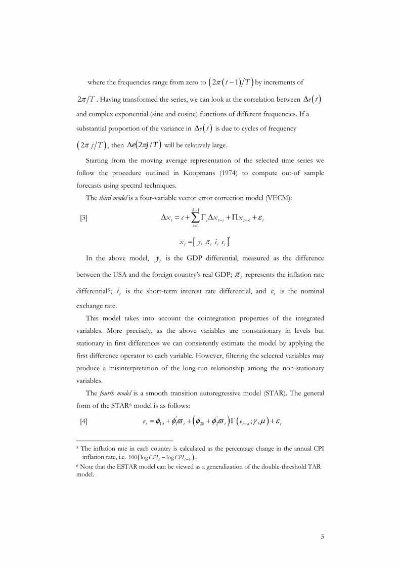
where the frequencies range from zero to ( )( )2 1t Tπ − by increments of

2 Tπ . Having transformed the series, we can look at the correlation between ( )e tΔ

and complex exponential (sine and cosine) functions of different frequencies. If a

substantial proportion of the variance in ( )e tΔ is due to cycles of frequency

( )2 j Tπ , then ( )Tje /2πΔ will be relatively large.

Starting from the moving average representation of the selected time series we

follow the procedure outlined in Koopmans (1974) to compute out-of sample

forecasts using spectral techniques.

The third model is a four-variable vector error correction model (VECM):

[3] ε−

− −=

Δ = + Γ Δ +Π +∑1

1

k

t i t i t k ti

x c x x

[ ]π ′= t t t t tx y i e

In the above model, ty is the GDP differential, measured as the difference

between the USA and the foreign country’s real GDP; tπ represents the inflation rate

differential TPF

5FPT; ti is the short-term interest rate differential, and te is the nominal

exchange rate.

This model takes into account the cointegration properties of the integrated

variables. More precisely, as the above variables are nonstationary in levels but

stationary in first differences we can consistently estimate the model by applying the

first difference operator to each variable. However, filtering the selected variables may

produce a misinterpretation of the long-run relationship among the non-stationary

variables.

The fourth model is a smooth transition autoregressive model (STAR). The general

form of the STARTPF

6FPT model is as follows:

[4] ( ) ( )' '10 1 20 2 ; ,t t t t d te eφ φϖ φ φ ϖ γ μ ε−= + + + Γ +

TP

5PT The inflation rate in each country is calculated as the percentage change in the annual CPI

inflation rate, i.e. ( )−− 4100 log logt tCPI CPI . TP

6PT Note that the ESTAR model can be viewed as a generalization of the double-threshold TAR

model.

6

where { }te is a stationary and ergodic process, ( )ϖ − −= 1 , ........,t t t pe e a vector of

lagged values, ε σ∼ 2(0, )t iid . The transition function ( )γ μ−Γ ; ,t de depends on a

transition variable ( t de − ), the speed of adjustment parameter 0γ > , and the

equilibrium parameter c. In general, the transition function may have two different

forms:

[5] ( ) ( ){ } 1

1 ; , 1 expt d t de eγ μ γ μ−

− −Γ = + ⎡− − ⎤⎣ ⎦

[6] ( ) ( )22 ; , 1 expt d t de eγ μ γ μ− −

⎡ ⎤Γ = − − −⎣ ⎦

where the first equation describes a logistic function (LSTAR) and the second one

represents an exponential function (ESTAR). The specific form of the transition

function is usually tested by employing a battery of tests proposed by Granger and

Teräsvirta (1993). However, in our case we directly estimate the model in its ESTAR

form. In fact, the ESTAR model is more suitable than the LSTAR framework in

analyzing the dynamic behaviour of the exchange rate deviations from equilibrium.

This is so because the symmetry of the exponential transition function Γ2 around μ

implies a symmetric behaviour of the exchange rate adjustment regardless of whether

the deviation form equilibrium is positive or negative. This means that the class of

model used in the present study is:

[7] ( ) ( ){ } ( )2 *

1 1

1 expp p

t i t i t d i t i ti i

e e e eμ α μ γ μ α μ ε− − −= =

⎡ ⎤Δ = + Δ − + − − − Δ − +⎣ ⎦∑ ∑

This transition function has a minimum of zero at t de μ− = and approaches unity

as t de μ− − → ±∞ . As a consequence, the ESTAR model is in the first regime when

t de − is close to μ and in the second regime when deviations of t de − from its

equilibrium value (in both direction) are large. Within each regime, the exchange rate

reverts to a linear autoregressive representation, with different parameter values and

asymmetric speeds of adjustment.

The specific form used in the analysis is:

[8] ( ) ( ){ } ( )4

2 *1 1

1

1 expt t t i t i ti

e e e eμ μ γ μ α μ ε− − −=

⎡ ⎤Δ = + Δ − + − − − Δ − +⎣ ⎦ ∑

7

The fifth model is a univariate Markov-switching model (MS-AR) similar to the one

estimated by Engel and Hamiltom (1990). In this model, the dynamics of discrete

shifts follows a two-state Markov process with an AR(4) component. The lag

structure has been tested with standard AIC, HQ and SC criteria. These statistics

suggest an autoregressive structure of order four. The model has the form:

[9] ( )μ α μ ε− −=

Δ − = Δ − +∑4

1

( ) ( )t t i t i t i ti

e s e s

where ε σ∼ 2(0, )t NID and the conditional mean )( tsμ switches between two

states:

μμ

μ> =⎧

= ⎨ < =⎩1

1

0 if 1 ( )

0 if 2 t

tt

ss

s

ts is a generic ergodic Markov chain defined by the transition probabilities:

( )+=

= = = = ∀ ∈∑11

Pr | , 1 , {1, 2}M

ij t t iji

p s j s i p i j . The transition probabilities

express the probability of moving from one state to another. Our hypothesis is that

the above process follows a two-state Markov chain. It is then possible to express the

transition probabilities in a ×2 2 transition matrix: ⎡ ⎤

= ⎢ ⎥⎣ ⎦

11 12

21 22

p pP

p p, where ijp

represents the probability of moving from state i to state j. In other words, 12p is the

fraction of the times that the system in state 1 moves to state 2. Estimating a Markov-

switching model involves an estimation of all the parameters and the hidden Markov

chain followed by the regimes. Maximum likelihood estimates of the model can be

recovered by performing a numerical maximization technique as described in Berndt

et al.(1974).

The sixth model consists of a Markov switching VECM (MS-VECM). As in the

linear case, it is made up of four variables (y, π , i and e). Following the two-stage

procedure suggested by Krolzig (1997) the results obtained in the linear VECM

concerning the cointegration analysis are used in this stage of the analysis.

The hypothesis behind the specific form of the estimated model is that the

dynamics of the exchange rate process follows a 3-state Markov chain. The idea is that

8

the relation between the exchange rate and the fundamentals is time-varying but

constant conditional on the stochastic and unobservable regime variable. More

specifically, the model allows for an unrestricted shift in the intercept and the

variance-covariance matrix and for two lags in each variableTP

PTTPF

7FPT:

[10] αβ ε−

− −=

Δ = + Γ Δ + +∑1

'

1

( )k

t t i t i t k ti

x c s x x

[ ]π ′= t t t t tx y i e

where the residuals are conditionally Gaussian, ( )( )ε ∼ Σ0,t t ts NID s .

The seventh model accounts for the time varying forecast ability of alternative

models. The idea behind combining forecasting techniques is straightforward: no

forecasting method is appropriate for all situations. This means that single forecasting

models may be optimal only conditional on a given sample realization, information

set, model specification or time periods. By implementing a combination of methods,

we can compensate the weakness of a forecasting model under particular conditions.

Altough the theoretical literatureTPF

8FPT suggests that appropriate combinations of

individual forecasts often have superior performance, such methods have not been

widely exploited in the empirical exchange rate literature (see the recent study of Sarno

and Valente (2005) however).. In the present study we compute combined forecasts

using the methodology proposed in Hong and Lee (2003), Yang (2004) and Yang and

Zou (2004).

Denoting kte the exchange rate forecast series obtained from model k, where

k=1,…,6 represents the six models outlined above (i.e. RW, SP, MS-AR, VECM, MS-

VECM, ESTAR) the combined forecast is obtained as:

[11] ω=

=∑6

*

1

k kt kt t

i

e e

TP

7PT We also estimated the model allowing for a shift in the mean of the variables. The results we

obtained from the two specifications are very similar with respect to the regime classification as well as to the parameter values. As we expected, the differences between the two models mainly consist of the different pattern of the dynamic propagation of a permanent shift in regime. More precisely, in the MSIH model, the expected growth of the variables responds to a transition from one state to another in a smoother way. See Krolzig (1997) on the peculiarity of the two models. TP

8PT See for example Bates and Granger (1969), Granger and Ramanathan (1984) and Clemen

(1989).

9

where the weights ( ktω ) attached to each model are calculated as follows:

[12]

( )

( )

21

21

26 1

21 1

1exp2

1exp2

ktj j

j t

ktkt

j j

k j t

e e

e e

σω

σ

−

=

−

= =

⎡ ⎤−⎢ ⎥−⎢ ⎥⎣ ⎦=⎡ ⎤−⎢ ⎥−⎢ ⎥⎣ ⎦

∑

∑ ∑

where σ 2t is the actual conditional variance of the exchange rate.

The specific relationship imposed ensures that a weight attributed to a certain

model at time t is larger the larger has been its ability to forecast the actual exchange

rate in period t-1. Figure 1 shows the weights used in computing the combined

forecast series.

Visual inspection provides useful information concerning the time-varying forecast

abilities of competing models. A situation where the weights attributed to each model

are very similar, as in the central part of the sample period for the 1-quarter-ahead

forecast of the pound, suggests that the relative accuracy of the forecasts produced by

each model may not be affected by a particular sub-sample period selected by the

evaluation strategy. Moreover, the results obtained with one model are not different

from the others. When, instead, weights are very dissimilar, a correct choice of the

forecasting model may produce a significant improvement in terms of predictive

accuracy.

The figure also suggests that there is a positive relationship between the volatility

of the selected weights, i.e. the number of time each model account for the same

proportion in the combing series, and the forecasting horizon.

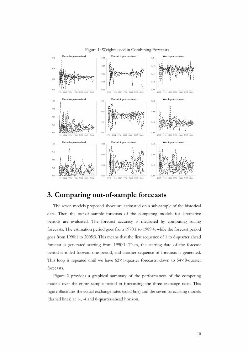
10

Figure 1: Weights used in Combining Forecasts Euro: 1-quarter-ahead

1992 1994 1996 1998 2000 2002 20040.00

0.14

0.28

0.42

Euro: 4-quarter-ahead

1992 1994 1996 1998 2000 2002 20040.00

0.25

0.50

0.75

1.00


1992 1994 1996 1998 2000 2002 20040.00

0.25

0.50

0.75

1.00

Pound: 1-quarter-ahead

1992 1994 1996 1998 2000 2002 20040.00

0.08

0.16

0.24

0.32


1992 1994 1996 1998 2000 2002 20040.0

0.1

0.2

0.3


1992 1994 1996 1998 2000 2002 20040.00

0.16

0.32

0.48

Yen: 1-quarter-ahead

1992 1994 1996 1998 2000 2002 20040.09

0.12

0.15

0.18

0.21


1992 1994 1996 1998 2000 2002 20040.00

0.18

0.36

0.54


1992 1994 1996 1998 2000 2002 20040.00

0.18

0.36

0.54

3. Comparing out-of-sample forecasts

The seven models proposed above are estimated on a sub-sample of the historical

data. Then the out-of sample forecasts of the competing models for alternative

periods are evaluated. The forecast accuracy is measured by computing rolling

forecasts. The estimation period goes from 1970:1 to 1989:4, while the forecast period

goes from 1990:1 to 2005:3. This means that the first sequence of 1 to 8-quarter ahead

forecast is generated starting from 1990:1. Then, the starting date of the forecast

period is rolled forward one period, and another sequence of forecasts is generated.

This loop is repeated until we have 62×1-quarter forecasts, down to 54×8-quarter

forecasts.

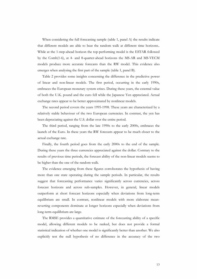
Figure 2 provides a graphical summary of the performances of the competing

models over the entire sample period in forecasting the three exchange rates. This

figure illustrates the actual exchange rates (solid line) and the seven forecasting models

(dashed lines) at 1-, -4 and 8-quarter-ahead horizon.

11

Visual inspection suggests a better performance, in terms of forecast errors, of

short-horizon exchange rates forecasts. However, the figure also illustrates higher

long-horizon forecast volatility. This means that the gains (but also the losses) we can

achieve by using a particular model are larger the longer is the forecasting horizon.

However, in order to assess the performance of the alternative models we have to

analyse the forecast accuracy through a set of statistical measures.

Figure 2: Out-of-sample Point Forecasts of competing models


1992 1994 1996 1998 2000 2002 2004-50

-25

0

25


1992 1994 1996 1998 2000 2002 2004-60

-30

0

30

60


1992 1994 1996 1998 2000 2002 2004-50

-25

0

25


1992 1994 1996 1998 2000 2002 2004-72

-60

-48

-36

-24


1992 1994 1996 1998 2000 2002 2004-80

-60

-40

-20


1992 1994 1996 1998 2000 2002 2004-70

-60

-50

-40

-30


1992 1994 1996 1998 2000 2002 2004432

450

468

486

504


1992 1994 1996 1998 2000 2002 2004425

450

475

500


1992 1994 1996 1998 2000 2002 2004420

450

480

510

4. Measuring forecast accuracy The aim of this section is to examine the out-of-sample forecasting performance

of alternative exchange rates models. Once each model has been estimated, the

question arises as to how their performance may best be compared. In principle,

forecast accuracy of competing models may be evaluated by employing various

econometric procedures. Starting from the out-of-sample prediction errors, this paper

12

computes three statistical measures – point forecasts, forecast encompassing tests and

directional accuracy tests.

4.1 Point Forecasts Evaluation

We first use standard quantitative procedures involving forecast errors. The

forecast error can be defined as: $ ++ += − t kt k t ke x x , where ≥ 1k and $ +t hx represents

the k-step-ahead forecast. The most widely used measure of forecast accuracy is the

Root Mean Square Error (RMSE) . We can calculate it as follows:

[13] + +=

⎛ ⎞= ⎜ ⎟⎝ ⎠∑

1/22

1

1 n

t k ii

RMSE en

The comparison of forecasting performance based on this measure is summarized

in Tables 1 and 2.

Each table characterizes some periods of the three exchange rates histories. Table

1 analyses the periods 1992-2005 and 1991-1998. The four periods described in table 2

are 1992-1995, 1995-1998, 1998-2001, and 2001-2005.

These tables also illustrate the relative ranking in terms of forecast errors for the

126 cases (seven models, three horizons, six sub-samples). The last column in each

table reports the average ranks of the model over the three exchange rates.

Table 1: Comparing Forecast Accuracy

Panel A: 1992:1-2005:2 Panel B: 1992:1-1998:4Euro Rank Pound Rank Yen Rank Avg. Rank Euro Rank Pound Rank Yen Rank Avg. Rank

1-quarter 1-quarterRW 4.16 [1] 3.66 [3] 5.10 [4] [2.7] RW 4.59 [1] 4.84 [2] 5.01 [4] [2.3]SP 4.40 [4] 3.66 [2] 5.09 [3] [3.0] SP 4.96 [3] 4.81 [1] 5.31 [5] [3.0]MS(2)-AR(4) 5.76 [5] 5.29 [6] 6.05 [6] [5.7] MS(2)-AR(4) 6.33 [5] 6.84 [6] 6.20 [6] [5.7]MS(3)-VEC(4) 6.54 [7] 5.82 [7] 6.43 [7] [7.0] MS(3)-VEC(4) 8.20 [7] 6.97 [7] 6.46 [7] [7.0]ESTAR 4.28 [3] 3.63 [1] 5.02 [2] [2.0] ESTAR 4.74 [2] 4.91 [3] 4.99 [3] [2.7]VEC(4) 6.41 [6] 5.10 [5] 5.19 [5] [5.3] VEC(4) 6.88 [6] 5.11 [4] 4.91 [2] [4.0]Comb(1-6) 4.36 [2] 3.98 [4] 4.94 [1] [2.3] Comb(1-6) 5.08 [4] 5.12 [5] 4.93 [1] [3.3]4-quarter 4-quarterRW 9.97 [3] 7.74 [2] 10.69 [3] [2.7] RW 9.04 [2] 8.55 [2] 11.13 [3] [2.3]SP 11.60 [5] 8.93 [6] 13.03 [7] [6.0] SP 11.23 [4] 9.84 [5] 13.82 [7] [5.3]MS(2)-AR(4) 10.97 [4] 8.45 [4] 11.93 [5] [4.3] MS(2)-AR(4) 11.44 [5] 10.04 [6] 13.34 [6] [5.7]MS(3)-VEC(4) 17.10 [6] 10.90 [7] 11.99 [6] [6.3] MS(3)-VEC(4) 20.90 [6] 12.71 [7] 13.14 [5] [6.0]ESTAR 9.88 [2] 7.89 [3] 11.46 [4] [3.0] ESTAR 9.74 [3] 9.00 [3] 11.47 [4] [3.3]VEC(4) 18.10 [7] 8.79 [5] 10.13 [2] [4.7] VEC(4) 22.17 [7] 9.01 [4] 10.94 [2] [4.3]Comb(1-6) 9.14 [1] 7.45 [1] 9.87 [1] [1.0] Comb(1-6) 8.95 [1] 8.43 [1] 10.56 [1] [1.0]8-quarter 8-quarterRW 15.23 [5] 11.47 [6] 16.53 [5] [5.3] RW 11.59 [4] 20.62 [6] 161.55 [4] [4.7]SP 15.61 [6] 11.67 [7] 17.72 [6] [6.3] SP 13.06 [5] 21.51 [7] 161.71 [6] [6.0]MS(2)-AR(4) 10.46 [2] 8.13 [2] 11.51 [3] [2.3] MS(2)-AR(4) 10.82 [3] 19.66 [4] 161.02 [2] [3.0]MS(3)-VEC(4) 14.29 [4] 8.57 [3] 11.29 [2] [3.0] MS(3)-VEC(4) 16.32 [7] 19.65 [3] 160.96 [7] [5.7]ESTAR 11.41 [3] 10.89 [5] 18.00 [7] [5.0] ESTAR 9.95 [2] 20.45 [5] 161.63 [5] [4.0]VEC(4) 17.47 [7] 9.66 [4] 16.64 [4] [5.0] VEC(4) 16.06 [6] 19.52 [2] 161.49 [3] [3.7]Comb(1-6) 9.80 [1] 7.28 [1] 10.51 [1] [1.0] Comb(1-6) 9.42 [1] 18.97 [1] 160.93 [1] [1.0]

13

When considering the full forecasting sample (table 1, panel A) the results indicate

that different models are able to beat the random walk at different time horizons..

While at the 1-step-ahead horizon the top-performing model is the ESTAR followed

by the Comb(1-6), at 4- and 8-quarter-ahead horizons the MS-AR and MS-VECM

models produce more accurate forecasts than the RW model. This evidence also

emerges when analysing the first part of the sample (table 1, panel B).

Table 2 provides some insights concerning the difference in the predictive power

of linear and non-linear models. The first period, occurring in the early 1990s,

embraces the European monetary system crises. During these years, the external value

of both the U.K. pound and the euro fell while the Japanese Yen appreciated. Actual

exchange rates appear to be better approximated by nonlinear models.

The second period covers the years 1995-1998. These years are characterized by a

relatively stable behaviour of the two European currencies. In contrast, the yen has

been depreciating against the U.S. dollar over the entire period.

The third period, ranging from the late 1990s to the early 2000s, embraces the

launch of the Euro. In these years the RW forecasts appear to be much closer to the

actual exchange rate.

Finally, the fourth period goes from the early 2000s to the end of the sample.

During these years the three currencies appreciated against the dollar. Contrary to the

results of previous time periods, the forecast ability of the non-linear models seems to

be higher than the one of the random walk.

The evidence emerging from these figures corroborates the hypothesis of having

more than one state operating during the sample periods. In particular, the results

suggest that forecasting performance varies significantly across currencies, across

forecast horizons and across sub-samples. However, in general, linear models

outperform at short forecast horizons especially when deviations from long-term

equilibrium are small. In contrast, nonlinear models with more elaborate mean-

reverting components dominate at longer horizons especially when deviations from

long-term equilibrium are large. The RMSE provides a quantitative estimate of the forecasting ability of a specific

model, allowing different models to be ranked, but does not provide a formal

statistical indication of whether one model is significantly better than another. We also

explicitly test the null hypothesis of no difference in the accuracy of the two

14

competing forecasts by using forecast encompassing tests. In particular, we use a

modified version of the Diebold-Mariano (1995) forecast comparison tests.

Table 2: Comparing Forecast Accuracy Panel A: 1992:1-1995:1 Panel B: 1995:1 - 1998:1

Euro Rank Pound Rank Yen Rank Avg. Rank Euro Rank Pound Rank Yen Rank Avg. Rank1-quarter 1-quarterRW 5.70 [2] 6.79 [2] 3.92 [4] [2.7] RW 3.26 [1] 1.79 [2] 6.10 [1] [1.3]SP 5.77 [3] 6.48 [1] 3.97 [5] [3.0] SP 4.11 [5] 2.01 [4] 6.42 [4] [4.3]MS(2)-AR(4) 8.27 [6] 9.70 [7] 5.29 [7] [6.7] MS(2)-AR(4) 4.04 [4] 2.03 [5] 7.37 [6] [5.0]MS(3)-VEC(4) 10.37 [7] 9.33 [6] 4.25 [6] [6.3] MS(3)-VEC(4) 5.71 [7] 3.42 [7] 8.42 [7] [7.0]ESTAR 6.10 [4] 6.95 [4] 3.69 [3] [3.7] ESTAR 3.07 [2] 1.85 [3] 6.26 [3] [2.7]VEC(4) 7.63 [5] 7.03 [5] 3.12 [1] [3.7] VEC(4) 4.91 [6] 2.06 [6] 6.46 [5] [5.7]Comb(1-6) 5.61 [1] 6.91 [3] 3.58 [2] [2.0] Comb(1-6) 3.61 [3] 1.62 [1] 6.25 [2] [2.0]4-quarter 4-quarterRW 9.18 [1] 11.62 [3] 9.92 [5] [3.0] RW 9.11 [4] 4.35 [2] 12.62 [2] [2.7]SP 10.80 [2] 11.98 [4] 12.04 [7] [4.3] SP 12.08 [5] 6.42 [5] 15.56 [5] [5.0]MS(2)-AR(4) 13.45 [5] 13.46 [6] 9.19 [4] [5.0] MS(2)-AR(4) 8.75 [3] 5.40 [4] 17.23 [6] [4.3]MS(3)-VEC(4) 20.59 [6] 16.93 [7] 7.72 [2] [5.0] MS(3)-VEC(4) 16.87 [7] 7.55 [7] 17.60 [7] [7.0]ESTAR 11.42 [4] 12.36 [5] 10.75 [6] [5.0] ESTAR 7.25 [2] 4.66 [3] 12.17 [1] [2.0]VEC(4) 29.45 [7] 11.30 [1] 7.10 [1] [3.0] VEC(4) 12.13 [6] 6.58 [6] 14.38 [4] [5.3]Comb(1-6) 11.34 [3] 11.39 [2] 8.51 [3] [2.7] Comb(1-6) 5.40 [1] 4.07 [1] 13.00 [3] [1.7]8-quarter 8-quarterRW 11.32 [3] 29.42 [6] 236.15 [5] [4.7] RW 12.23 [4] 4.29 [2] 19.11 [5] [3.7]SP 11.92 [4] 30.30 [7] 236.21 [6] [5.7] SP 14.58 [5] 8.17 [7] 20.55 [6] [6.0]MS(2)-AR(4) 13.16 [5] 28.09 [3] 235.73 [3] [3.7] MS(2)-AR(4) 8.31 [1] 6.14 [5] 16.46 [3] [3.0]MS(3)-VEC(4) 15.46 [7] 28.27 [4] 235.70 [2] [4.3] MS(3)-VEC(4) 15.79 [6] 5.63 [3] 15.68 [2] [3.7]ESTAR 10.15 [1] 28.98 [5] 236.29 [7] [4.3] ESTAR 10.42 [3] 5.98 [4] 17.88 [4] [3.7]VEC(4) 14.95 [6] 27.41 [2] 235.82 [4] [4.0] VEC(4) 16.19 [7] 7.27 [6] 23.17 [7] [6.7]Comb(1-6) 10.89 [2] 19.38 [1] 234.74 [1] [1.3] Comb(1-6) 8.45 [2] 3.51 [1] 13.21 [1] [1.3]

Panel C: 1998:1 - 2001:1 Panel D: 2001:1-2005:2Euro Rank Pound Rank Yen Rank Avg. Rank Euro Rank Pound Rank Yen Rank Avg. Rank

1-quarter 1-quarterRW 4.14 [2] 2.13 [1] 6.10 [5] [2.7] RW 4.35 [3] 2.94 [2] 4.11 [3] [2.7]SP 4.45 [4] 2.18 [2] 5.74 [1] [2.3] SP 4.35 [4] 2.96 [3] 4.19 [5] [4.0]MS(2)-AR(4) 4.22 [3] 2.19 [3] 7.10 [6] [4.0] MS(2)-AR(4) 5.94 [6] 3.62 [5] 4.13 [4] [5.0]MS(3)-VEC(4) 4.33 [4] 4.77 [7] 7.79 [7] [6.0] MS(3)-VEC(4) 5.13 [5] 3.97 [6] 4.31 [6] [5.7]ESTAR 4.52 [5] 2.28 [5] 5.94 [4] [4.7] ESTAR 4.21 [2] 2.54 [1] 3.81 [2] [1.7]VEC(4) 4.84 [6] 2.81 [6] 5.63 [2] [4.7] VEC(4) 7.79 [7] 6.35 [7] 4.77 [7] [7.0]Comb(1-6) 3.85 [1] 2.26 [4] 5.84 [3] [2.7] Comb(1-6) 4.42 [1] 3.20 [4] 3.80 [1] [2.0]4-quarter 4-quarterRW 9.73 [3] 5.26 [4] 11.54 [3] [2.3] RW 10.69 [5] 7.85 [4] 8.20 [3] [4.3]SP 12.77 [6] 4.88 [1] 12.55 [5] [5.3] SP 10.68 [4] 8.93 [5] 12.31 [7] [4.7]MS(2)-AR(4) 9.03 [1] 5.83 [5] 11.69 [4] [3.0] MS(2)-AR(4) 10.83 [6] 7.81 [3] 8.38 [5] [6.0]MS(3)-VEC(4) 10.59 [4] 8.40 [4] 12.77 [7] [5.7] MS(3)-VEC(4) 11.44 [7] 9.78 [7] 8.33 [4] [4.0]ESTAR 11.75 [5] 7.28 [6] 12.35 [6] [4.7] ESTAR 8.07 [1] 7.24 [1] 9.15 [6] [4.3]VEC(4) 14.08 [7] 5.10 [3] 11.17 [2] [3.7] VEC(4) 9.78 [3] 9.71 [6] 7.35 [1] [2.0]Comb(1-6) 9.22 [2] 4.90 [2] 10.14 [1] [1.7] Comb(1-6) 8.57 [2] 7.60 [2] 7.68 [2] [2.0]8-quarter 8-quarterRW 15.09 [5] 7.37 [5] 16.65 [5] [5.0] RW 19.95 [7] 13.70 [7] 11.94 [4] [6.0]SP 17.01 [7] 7.30 [4] 13.97 [4] [5.0] SP 19.61 [5] 13.01 [6] 16.10 [7] [6.0]MS(2)-AR(4) 9.48 [1] 5.42 [2] 12.28 [3] [2.0] MS(2)-AR(4) 11.88 [1] 8.46 [1] 7.92 [1] [1.0]MS(3)-VEC(4) 12.12 [3] 6.32 [3] 12.11 [2] [2.7] MS(3)-VEC(4) 12.88 [3] 9.36 [3] 8.98 [3] [3.0]ESTAR 13.12 [4] 9.08 [7] 17.54 [7] [6.0] ESTAR 13.52 [4] 11.96 [4] 14.29 [6] [4.7]VEC(4) 16.81 [6] 7.56 [6] 17.12 [6] [6.0] VEC(4) 19.77 [6] 12.00 [5] 13.83 [5] [5.3]Comb(1-6) 9.98 [2] 4.52 [1] 9.74 [1] [1.3] Comb(1-6) 12.01 [2] 9.03 [2] 8.96 [2] [2.0]

More precisely, the accuracy of the alternative forecasts can be judged according to

some loss function, (.)g . In analysing formal tests of the null hypothesis of equal

forecast accuracy, we follow Diebold and Mariano (1995) and define the loss function

as a function of the forecast errors. The loss differential is then denoted as

15

= −1 2( ) ( )t t td g e g e TPF

9FPT, where 1te and 2te are the forecast errors at time t of the model 1

and 2. The null hypothesis of unconditional equal forecast accuracy in this context is

that the loss differential has mean 0, i.e. =0 : [ ] 0tH E d . According to the null

hypothesis the errors associated with the two forecasts are equally costly, on average.

If the null is rejected, the forecasting method that yields the smallest loss is preferred.

Given a series, =1{ }Tt td , of loss differentials, the test of forecast accuracy is based on:

[14] =

= ∑1

1 T

tt

d dT

The Diebold and Mariano (1995) (DM) parametric test is a well-known procedure

for testing the null hypothesis of no difference in the accuracy of two competing

forecasts. It is given by:

[15] ( ) ( )( )1

( 1) 2

( 1) 1

2 / ( )T T

t tT t

DM d l s t d d d dττ τ

π τ−

−

−=− − = +

⎡ ⎤= + −⎢ ⎥

⎢ ⎥⎣ ⎦∑ ∑

where ( )/ ( )l s tτ is the lag windowTPF

10FPT, ( )s t is the truncation lag and T the number

of observations. Harvey, et al. (1997) propose a modified version of the Diebold-

Mariano test statistic in order to adjust for the possible wrong size of the original test

when the forecasting horizon, k increases. The statistic they proposed is:

[16] ( )11 1 22 1 2 1MDM T T k T k k DM− −⎡ ⎤= + − + −⎣ ⎦

We follow the suggestion of Harvey et al. (1997) in comparing the statistics with

critical values from the Student’s t distribution with (T-1) degrees of freedom, rather

than from the standard normal distribution.

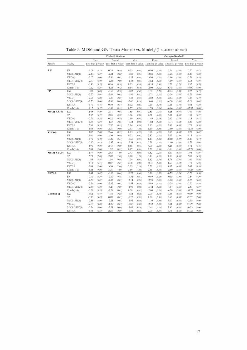
Table 3 to 5 report the modified DM and the Granger and Newbold TPF

11FPT test

statistics of equal forecast accuracy (as measured by MSE) and the associated

probabilities under the null (of equal accuracy). P-values (in square brackets) no

greater the 0.05 suggest that Model i produces a lower forecast error (in terms of root

TP

9PT The loss function is defined as = −2 2

1 2( ) ( )t t td g e g e and = −1 2( ) ( )t t td g e g e for MSE and MAE, respectively.

TP

10PT This term is computed by using the Newey-West lag window.

TP

11PT See Granger and Newbold (1976) for a detailed description of the test.

16

mean squared error) relative to the Model j at the 5% significance level. In contrast, p-

values no smaller then 0.95 mean that Model i generates a higher forecast error at the

5% level.

In absolute terms, if we consider the number of times each model significantly

beats its competitors according to the two test statistics, we have different results

depending on the forecast horizon. More precisely, at 1-quarter-ahead horizon,

ESTAR models outperform the others 50% of the times. At 4- and 8- quarter

horizon, combined forecasts are found to be the top-performing models. Of a total of

18 cases (six competitors for each of the three currencies), the percentage of times the

combined forecast models beat the other models is higher than 60%. This evidence is

in line with the results obtained with the RMSE in table 1 and 2.

17

Table 3: MDM and GN Tests: Model i vs. Model j (1-quarter-ahead)

Model i Model j Test Stat p-value Test Stat p-value Test Stat p-value Test Stat p-value Test Stat p-value Test Stat p-value

RW SP -1.08 [0.14] 0.25 [0.50] 0.03 [0.51] -0.80 [0.21] 0.24 [0.60] -0.22 [0.41]MS(2)-AR(4) -2.43 [0.01] -2.11 [0.02] -1.85 [0.03] -2.83 [0.00] -3.25 [0.00] -1.40 [0.08]VEC(4) -3.07 [0.00] -2.46 [0.01] -0.23 [0.41] -3.96 [0.00] -2.86 [0.00] -0.28 [0.39]MS(3)-VEC(4) -2.77 [0.00] -2.83 [0.00] -2.43 [0.01] -3.52 [0.00] -4.19 [0.00] -1.98 [0.03]ESTAR -0.43 [0.33] 0.16 [0.56] 0.25 [0.60] -0.18 [0.43] 0.72 [0.76] 0.52 [0.70]Comb(1-6) -0.62 [0.27] -1.18 [0.12] 0.54 [0.70] -2.00 [0.02] -6.45 [0.00] -49.09 [0.00]

SP RW 1.08 [0.86] -8.50 [0.50] -0.03 [0.49] 0.80 [0.79] -0.24 [0.40] 0.22 [0.59]MS(2)-AR(4) -2.37 [0.01] -2.04 [0.02] -1.96 [0.02] -2.71 [0.00] -3.34 [0.00] -1.39 [0.09]VEC(4) -2.91 [0.00] -2.30 [0.01] -0.32 [0.37] -3.82 [0.00] -2.63 [0.01] -0.15 [0.44]MS(3)-VEC(4) -2.73 [0.00] -2.69 [0.00] -2.60 [0.00] -3.44 [0.00] -4.38 [0.00] -2.08 [0.02]ESTAR 0.71 [0.76] 0.10 [0.54] 0.32 [0.63] 0.69 [0.75] 0.15 [0.56] 0.84 [0.80]Comb(1-6) 0.17 [0.57] -0.89 [0.19] 0.77 [0.78] -1.78 [0.04] -6.66 [0.00] -47.97 [0.00]

MS(2)-AR(4) RW 2.43 [0.99] 2.11 [0.98] 1.85 [0.97] 2.83 [1.00] 3.25 [1.00] 1.40 [0.92]SP 2.37 [0.99] 2.04 [0.98] 1.96 [0.98] 2.71 [1.00] 3.34 [1.00] 1.39 [0.91]VEC(4) -0.76 [0.22] 0.22 [0.59] 1.60 [0.95] -1.43 [0.08] 0.60 [0.73] 1.14 [0.87]MS(3)-VEC(4) -1.85 [0.03] -1.54 [0.06] -1.34 [0.09] -1.82 [0.04] -1.74 [0.04] -1.40 [0.08]ESTAR 2.50 [0.99] 2.37 [0.99] 2.14 [0.98] 2.93 [1.00] 3.82 [1.00] 1.75 [0.96]Comb(1-6) 2.88 [1.00] 2.21 [0.99] 2.93 [1.00] 1.10 [0.86] -3.60 [0.00] -42.55 [0.00]

VEC(4) RW 3.07 [1.00] 2.46 [0.99] 0.23 [0.59] 3.96 [1.00] 2.86 [1.00] 0.28 [0.61]SP 2.91 [1.00] 2.30 [0.99] 0.32 [0.63] 3.82 [1.00] 2.63 [0.99] 0.15 [0.56]MS(2)-AR(4) 0.76 [0.78] -0.22 [0.41] -1.60 [0.05] 1.43 [0.92] -0.60 [0.27] -1.14 [0.13]MS(3)-VEC(4) -0.13 [0.45] -0.87 [0.19] -2.38 [0.01] 0.31 [0.62] -1.60 [0.06] -1.79 [0.04]ESTAR 2.96 [1.00] 2.43 [0.99] 0.55 [0.71] 4.09 [1.00] 3.28 [1.00] 0.72 [0.76]Comb(1-6) 2.89 [1.00] 1.92 [0.97] 0.87 [0.81] 2.52 [0.99] -3.81 [0.00] -47.79 [0.00]

MS(3)-VEC(4) RW 2.77 [1.00] 2.83 [1.00] 2.43 [0.99] 3.52 [1.00] 4.19 [1.00] 1.98 [0.97]SP 2.73 [1.00] 2.69 [1.00] 2.60 [1.00] 3.44 [1.00] 4.38 [1.00] 2.08 [0.98]MS(2)-AR(4) 1.85 [0.97] 1.54 [0.94] 1.34 [0.91] 1.82 [0.96] 1.74 [0.96] 1.40 [0.92]VEC(4) 0.13 [0.55] 0.87 [0.81] 2.38 [0.99] -0.31 [0.38] 1.60 [0.94] 1.79 [0.96]ESTAR 2.89 [1.00] 3.20 [1.00] 2.95 [1.00] 3.72 [1.00] 4.67 [1.00] 2.43 [0.99]Comb(1-6) 3.24 [1.00] 3.21 [1.00] 3.69 [1.00] 2.41 [0.99] -2.80 [0.00] -40.23 [0.00]

ESTAR RW 0.43 [0.67] -0.16 [0.44] -0.25 [0.40] 0.18 [0.57] -0.72 [0.24] -0.52 [0.30]SP -0.71 [0.24] -0.10 [0.46] -0.32 [0.37] -0.69 [0.25] -0.15 [0.44] -0.84 [0.20]MS(2)-AR(4) -2.50 [0.01] -2.37 [0.01] -2.14 [0.02] -2.93 [0.00] -3.82 [0.00] -1.75 [0.04]VEC(4) -2.96 [0.00] -2.43 [0.01] -0.55 [0.29] -4.09 [0.00] -3.28 [0.00] -0.72 [0.24]MS(3)-VEC(4) -2.89 [0.00] -3.20 [0.00] -2.95 [0.00] -3.72 [0.00] -4.67 [0.00] -2.43 [0.01]Comb(1-6) -0.38 [0.35] -2.24 [0.01] 0.38 [0.65] -2.00 [0.03] -6.78 [0.00] -51.72 [0.00]

Comb(1-6) RW 0.62 [0.73] 1.18 [0.88] -0.54 [0.30] 2.00 [0.98] 6.45 [1.00] 49.09 [1.00]SP -0.17 [0.43] 0.89 [0.81] -0.77 [0.22] 1.78 [0.96] 6.66 [1.00] 47.97 [1.00]MS(2)-AR(4) -2.88 [0.00] -2.21 [0.01] -2.93 [0.00] -1.10 [0.14] 3.60 [1.00] 42.55 [1.00]VEC(4) -2.89 [0.00] -1.92 [0.03] -0.87 [0.19] -2.52 [0.01] 3.81 [1.00] 47.79 [1.00]MS(3)-VEC(4) -3.24 [0.00] -3.21 [0.00] -3.69 [0.00] -2.41 [0.01] 2.80 [1.00] 40.23 [1.00]ESTAR 0.38 [0.65] 2.24 [0.99] -0.38 [0.35] 2.00 [0.97] 6.78 [1.00] 51.72 [1.00]

Diebold-Mariano Granger-Newbold Euro Pound Yen Euro Pound Yen

18



RW SP -2.30 [0.01] -1.99 [0.02] -2.44 [0.01] -2.50 [0.01] -0.57 [0.28] -0.08 [0.47]MS(2)-AR(4) -1.31 [0.10] -1.76 [0.04] -1.40 [0.08] -1.39 [0.08] -0.77 [0.22] 1.18 [0.88]VEC(4) -1.87 [0.03] -1.30 [0.10] 0.86 [0.81] -5.08 [0.00] 1.19 [0.88] 1.76 [0.96]MS(3)-VEC(4) -2.87 [0.00] -3.52 [0.00] -1.41 [0.08] -4.04 [0.00] -3.76 [0.00] 1.53 [0.93]ESTAR 0.12 [0.55] -0.43 [0.33] -1.21 [0.11] 0.00 [0.50] -1.63 [0.05] -1.14 [0.13]Comb(1-6) 1.37 [0.91] 1.61 [0.95] 2.49 [0.99] 1.23 [0.89] -2.19 [0.02] 1.41 [0.92]

SP RW 2.30 [0.99] 1.99 [0.98] 2.44 [0.99] 2.50 [0.99] 0.57 [0.72] 0.08 [0.53]MS(2)-AR(4) 0.55 [0.71] 0.63 [0.74] 0.80 [0.79] 0.66 [0.74] 0.06 [0.53] 0.69 [0.75]VEC(4) -1.58 [0.06] 0.15 [0.56] 2.22 [0.99] -3.25 [0.00] 1.10 [0.86] 0.90 [0.82]MS(3)-VEC(4) -2.24 [0.01] -1.82 [0.03] 0.75 [0.77] -2.47 [0.01] -1.92 [0.03] 0.82 [0.79]ESTAR 1.78 [0.96] 1.38 [0.92] 1.17 [0.88] 1.67 [0.95] -0.17 [0.43] -0.50 [0.31]Comb(1-6) 3.18 [1.00] 2.36 [0.99] 3.08 [1.00] 2.57 [0.99] -1.70 [0.05] 0.55 [0.71]

MS(2)-AR(4) RW 1.31 [0.90] 1.76 [0.96] 1.40 [0.92] 1.39 [0.92] 0.77 [0.78] -1.18 [0.12]SP -0.55 [0.29] -0.63 [0.26] -0.80 [0.21] -0.66 [0.26] -0.06 [0.47] -0.69 [0.25]VEC(4) -1.79 [0.04] -0.55 [0.29] 2.63 [1.00] -4.40 [0.00] 1.81 [0.96] 0.34 [0.63]MS(3)-VEC(4) -2.93 [0.00] -2.76 [0.00] -0.18 [0.43] -4.04 [0.00] -3.34 [0.00] 0.26 [0.60]ESTAR 1.19 [0.88] 1.13 [0.87] 0.43 [0.67] 1.20 [0.88] -0.48 [0.32] -1.91 [0.03]Comb(1-6) 2.38 [0.99] 2.86 [1.00] 2.63 [1.00] 2.57 [0.99] -1.73 [0.04] -0.55 [0.29]

VEC(4) RW 1.87 [0.97] 1.30 [0.90] -0.86 [0.19] 5.08 [1.00] -1.19 [0.12] -1.76 [0.04]SP 1.58 [0.94] -0.15 [0.44] -2.22 [0.01] 3.25 [1.00] -1.10 [0.14] -0.90 [0.18]MS(2)-AR(4) 1.79 [0.96] 0.55 [0.71] -2.63 [0.00] 4.40 [1.00] -1.81 [0.04] -0.34 [0.37]MS(3)-VEC(4) 0.33 [0.63] -1.71 [0.04] -2.85 [0.00] 0.49 [0.69] -3.74 [0.00] -0.25 [0.40]ESTAR 2.01 [0.98] 1.05 [0.85] -1.49 [0.07] 6.24 [1.00] -2.86 [0.00] -2.86 [0.00]Comb(1-6) 2.09 [0.98] 1.77 [0.96] 0.49 [0.69] 6.69 [1.00] -2.68 [0.00] -1.25 [0.11]

MS(3)-VEC(4) RW 2.87 [1.00] 3.52 [1.00] 1.41 [0.92] 4.04 [1.00] 3.76 [1.00] -1.53 [0.07]SP 2.24 [0.99] 1.82 [0.97] -0.75 [0.23] 2.47 [0.99] 1.92 [0.97] -0.82 [0.21]MS(2)-AR(4) 2.93 [1.00] 2.76 [1.00] 0.18 [0.57] 4.04 [1.00] 3.34 [1.00] -0.26 [0.40]VEC(4) -0.33 [0.37] 1.71 [0.96] 2.85 [1.00] -0.49 [0.31] 3.74 [1.00] 0.25 [0.60]ESTAR 3.03 [1.00] 3.37 [1.00] 0.46 [0.68] 4.15 [1.00] 2.51 [0.99] -2.20 [0.02]Comb(1-6) 3.27 [1.00] 3.82 [1.00] 2.62 [1.00] 5.80 [1.00] 0.32 [0.63] -0.88 [0.19]

ESTAR RW -0.12 [0.45] 0.43 [0.67] 1.21 [0.89] 0.00 [0.50] 1.63 [0.95] 1.14 [0.87]SP -1.78 [0.04] -1.38 [0.08] -1.17 [0.12] -1.67 [0.05] 0.17 [0.57] 0.50 [0.69]MS(2)-AR(4) -1.19 [0.12] -1.13 [0.13] -0.43 [0.33] -1.20 [0.12] 0.48 [0.68] 1.91 [0.97]VEC(4) -2.01 [0.02] -1.05 [0.15] 1.49 [0.93] -6.24 [0.00] 2.86 [1.00] 2.86 [1.00]MS(3)-VEC(4) -3.03 [0.00] -3.37 [0.00] -0.46 [0.32] -4.15 [0.00] -2.51 [0.01] 2.20 [0.98]Comb(1-6) 0.91 [0.82] 1.30 [0.90] 2.08 [0.98] 1.16 [0.87] -1.56 [0.06] 2.39 [0.99]

Comb(1-6) RW -1.37 [0.09] -1.61 [0.05] -2.49 [0.01] -1.23 [0.11] 2.19 [0.98] -1.41 [0.08]SP -3.18 [0.00] -2.36 [0.01] -3.08 [0.00] -2.57 [0.01] 1.70 [0.95] -0.55 [0.29]MS(2)-AR(4) -2.38 [0.01] -2.86 [0.00] -2.63 [0.00] -2.57 [0.01] 1.73 [0.96] 0.55 [0.71]VEC(4) -2.09 [0.02] -1.77 [0.04] -0.49 [0.31] -6.69 [0.00] 2.68 [1.00] 1.25 [0.89]MS(3)-VEC(4) -3.27 [0.00] -3.82 [0.00] -2.62 [0.00] -5.80 [0.00] -0.32 [0.37] 0.88 [0.81]ESTAR -0.91 [0.18] -1.30 [0.10] -2.08 [0.02] -1.16 [0.13] 1.56 [0.94] -2.39 [0.01]

Euro Pound Yen Euro Diebold-Mariano Granger-Newbold

Pound Yen

19



RW SP -0.51 [0.31] -0.31 [0.38] -1.06 [0.14] -0.69 [0.25] 1.29 [0.90] 0.41 [0.66]MS(2)-AR(4) 3.83 [1.00] 3.01 [1.00] 3.57 [1.00] 3.92 [1.00] 2.09 [0.98] 1.46 [0.92]VEC(4) -1.61 [0.05] 2.11 [0.98] -0.09 [0.46] -1.42 [0.08] 5.67 [1.00] 4.32 [1.00]MS(3)-VEC(4) 0.65 [0.74] 2.69 [1.00] 3.66 [1.00] 0.54 [0.70] 1.59 [0.94] 1.80 [0.96]ESTAR 3.79 [1.00] 0.92 [0.82] -1.54 [0.06] 3.79 [1.00] -1.46 [0.07] -2.91 [0.00]Comb(1-6) 5.50 [1.00] 5.42 [1.00] 6.89 [1.00] 6.00 [1.00] 3.12 [1.00] 1.55 [0.94]

SP RW 0.51 [0.69] 0.31 [0.62] 1.06 [0.86] 0.69 [0.75] -1.29 [0.10] -0.41 [0.34]MS(2)-AR(4) 4.02 [1.00] 3.93 [1.00] 3.90 [1.00] 3.81 [1.00] 1.20 [0.88] 0.87 [0.81]VEC(4) -1.39 [0.08] 2.51 [0.99] 0.64 [0.74] -1.10 [0.14] 2.99 [1.00] 1.87 [0.97]MS(3)-VEC(4) 0.86 [0.80] 3.42 [1.00] 4.02 [1.00] 0.77 [0.78] 0.71 [0.76] 1.16 [0.88]ESTAR 4.44 [1.00] 0.86 [0.80] -0.18 [0.43] 3.99 [1.00] -1.86 [0.03] -1.98 [0.03]Comb(1-6) 5.21 [1.00] 5.84 [1.00] 5.58 [1.00] 5.40 [1.00] 1.43 [0.92] 0.73 [0.77]

MS(2)-AR(4) RW -3.83 [0.00] -3.01 [0.00] -3.57 [0.00] -3.92 [0.00] -2.09 [0.02] -1.46 [0.08]SP -4.02 [0.00] -3.93 [0.00] -3.90 [0.00] -3.81 [0.00] -1.20 [0.12] -0.87 [0.19]VEC(4) -4.58 [0.00] -1.51 [0.07] -2.98 [0.00] -3.93 [0.00] 1.09 [0.86] 0.72 [0.76]MS(3)-VEC(4) -3.88 [0.00] -1.70 [0.04] 0.48 [0.68] -3.17 [0.00] -1.73 [0.04] 1.16 [0.88]ESTAR -0.76 [0.22] -2.57 [0.01] -3.65 [0.00] -0.84 [0.20] -3.13 [0.00] -3.59 [0.00]Comb(1-6) 0.95 [0.83] 1.06 [0.86] 1.02 [0.85] 0.76 [0.77] -0.11 [0.46] -0.70 [0.24]

VEC(4) RW 1.61 [0.95] -2.11 [0.02] 0.09 [0.54] 1.42 [0.92] -5.67 [0.00] -4.32 [0.00]SP 1.39 [0.92] -2.51 [0.01] -0.64 [0.26] 1.10 [0.86] -2.99 [0.00] -1.87 [0.03]MS(2)-AR(4) 4.58 [1.00] 1.51 [0.93] 2.98 [1.00] 3.93 [1.00] -1.09 [0.14] -0.72 [0.24]MS(3)-VEC(4) 2.19 [0.99] 1.01 [0.84] 3.17 [1.00] 1.49 [0.93] -1.58 [0.06] -0.41 [0.34]ESTAR 5.98 [1.00] -1.14 [0.13] -0.73 [0.23] 5.53 [1.00] -10.34 [0.00] -5.78 [0.00]Comb(1-6) 5.73 [1.00] 3.04 [1.00] 4.18 [1.00] 5.43 [1.00] -1.85 [0.03] -1.62 [0.06]

MS(3)-VEC(4) RW -0.65 [0.26] -2.69 [0.00] -3.66 [0.00] -0.54 [0.30] -1.59 [0.06] -1.80 [0.04]SP -0.86 [0.20] -3.42 [0.00] -4.02 [0.00] -0.77 [0.22] -0.71 [0.24] -1.16 [0.12]MS(2)-AR(4) 3.88 [1.00] 1.70 [0.96] -0.48 [0.32] 3.17 [1.00] 1.73 [0.96] -1.16 [0.12]VEC(4) -2.19 [0.01] -1.01 [0.16] -3.17 [0.00] -1.49 [0.07] 1.58 [0.94] 0.41 [0.66]ESTAR 1.92 [0.97] -2.21 [0.01] -3.53 [0.00] 1.44 [0.92] -2.47 [0.01] -3.90 [0.00]Comb(1-6) 3.90 [1.00] 1.61 [0.95] 0.75 [0.77] 3.26 [1.00] 0.85 [0.80] -1.36 [0.09]

ESTAR RW -3.79 [0.00] -0.92 [0.18] 1.54 [0.94] -3.79 [0.00] 1.46 [0.93] 2.91 [1.00]SP -4.44 [0.00] -0.86 [0.20] 0.18 [0.57] -3.99 [0.00] 1.86 [0.97] 1.98 [0.97]MS(2)-AR(4) 0.76 [0.78] 2.57 [0.99] 3.65 [1.00] 0.84 [0.80] 3.13 [1.00] 3.59 [1.00]VEC(4) -5.98 [0.00] 1.14 [0.87] 0.73 [0.77] -5.53 [0.00] 10.34 [1.00] 5.78 [1.00]MS(3)-VEC(4) -1.92 [0.03] 2.21 [0.99] 3.53 [1.00] -1.44 [0.08] 2.47 [0.99] 3.90 [1.00]Comb(1-6) 1.81 [0.96] 4.54 [1.00] 5.33 [1.00] 1.86 [0.97] 5.19 [1.00] 5.36 [1.00]

Comb(1-6) RW -5.50 [0.00] -5.42 [0.00] -6.89 [0.00] -6.00 [0.00] -3.12 [0.00] -1.55 [0.06]SP -5.21 [0.00] -5.84 [0.00] -5.58 [0.00] -5.40 [0.00] -1.43 [0.08] -0.73 [0.23]MS(2)-AR(4) -0.95 [0.17] -1.06 [0.14] -1.02 [0.15] -0.76 [0.23] 0.11 [0.54] 0.70 [0.76]VEC(4) -5.73 [0.00] -3.04 [0.00] -4.18 [0.00] -5.43 [0.00] 1.85 [0.97] 1.62 [0.94]MS(3)-VEC(4) -3.90 [0.00] -1.61 [0.05] -0.75 [0.23] -3.26 [0.00] -0.85 [0.20] 1.36 [0.91]ESTAR -1.81 [0.04] -4.54 [0.00] -5.33 [0.00] -1.86 [0.03] -5.19 [0.00] -5.36 [0.00]

Pound YenEuro Pound Yen Euro Diebold-Mariano Granger-Newbold

4.2 Forecasts Encompassing

Forecast encompassing assesses whether any extra important information is contained

in forecasts from rival models. A simple methodology to compare the forecast

accuracy has been developed by Fair-Shiller (1990). The testing procedure in the Fair-

Shiller approach is based on the following equation:

[17] ( ) ( )α α α ε− − −− = + − + − +$ $1, 2,1 2m t m tt t j m t j m t j te e e e e e j=1,4,8

where 1,m te$ , and 2,m te$ , are the forecasts obtained using model 1 (m1) and 2 (m2),

respectively. The intuition behind this testing procedure is straightforward. If both

forecasts contain useful and independent information concerning te , then the

20

estimates of the slope coefficients 1mα and 2mα should be significant. In contrast, if

the information in one forecast is completely contained in the other, then the

coefficient of the second forecast should be nonzero while that of the first one should

be zero.

The Fair-Shiller tests results are presented in tables 6, 7 and 8 for the dollar-euro,

dollar-pound and dollar-yen exchange rates, respectively. These tables report, for each

currency, regression coefficients from equation [17] and the associated t-values at

different horizons (1, 4 and 8 quarters ahead).

On the basis of the Fair-Shiller tests and with the notable exception of the

Japanese currency none of the selected models outperform their competitors at 1-

quarter-ahead horizon. It is interesting to note that when increasing the forecast

horizon, combined models dominate the others. In general, the longer the forecast

horizon, the worse the RW exchange rate forecasts become.

At 4-quarter-ahead horizon, combined forecasts still produce superior out-of-

sample forecasting performance compared to other models. However, in these cases,

other models also generate better forecasts if compared to the random walk. In fact,

the t-values of the ESTAR and VEC models are above the 95% confidence threshold

when compared with the RW, SP and MSAR models. From these tables, we can also

conclude that, in most cases, at the 8-querter horizon, the forecast accuracy of non-

linear models significantly outperforms that of the competing models.

21

Table 6: Dollar/Euro – Fair and Shiller encompassing test 1-quarter-ahead m1 m2

Coeff Tsta Coeff Tsta Coeff Tsta Coeff Tsta Coeff Tsta Coeff Tsta Coeff Tstac -0.03 -0.05 -0.07 -0.12 -0.02 -0.04 0.03 0.05 0.04 0.07 0.04 0.08α1 0.24 0.71 0.09 0.63 0.15 1.54 0.44 1.54 0.11 1.05 0.42 1.63α2 0.00 0.00 0.00 0.00 0.00 0.00 0.00 0.00 0.00 0.00 0.00 0.00c -0.03 -0.05 -0.05 -0.08 -0.02 -0.04 0.04 0.07 0.04 0.06 0.06 0.10α1 0.00 0.00 0.05 0.32 0.15 1.35 0.59 1.44 0.09 0.83 0.58 1.58α2 0.24 0.71 0.18 0.47 0.01 0.04 -0.24 -0.51 0.13 0.35 -0.30 -0.62c -0.07 -0.12 -0.05 -0.08 0.04 0.07 0.03 0.05 0.02 0.03 0.11 0.19α1 0.00 0.00 0.18 0.47 0.26 1.65 0.44 1.39 0.10 1.00 0.59 1.65α2 0.09 0.63 0.05 0.32 -0.20 -0.87 0.00 0.02 0.08 0.56 -0.14 -0.69c -0.02 -0.04 -0.02 -0.04 0.04 0.07 0.02 0.04 0.04 0.06 0.03 0.04α1 0.00 0.00 0.01 0.04 -0.20 -0.87 0.31 0.96 0.07 0.71 0.29 0.63α2 0.15 1.54 0.15 1.35 0.26 1.65 0.11 0.96 0.14 1.32 0.06 0.36c 0.03 0.05 0.04 0.07 0.03 0.05 0.02 0.04 0.07 0.12 0.05 0.09α1 0.00 0.00 -0.24 -0.51 0.00 0.02 0.11 0.96 0.06 0.55 0.28 0.77α2 0.44 1.54 0.59 1.44 0.44 1.39 0.31 0.96 0.38 1.24 0.23 0.56c 0.04 0.07 0.04 0.06 0.02 0.03 0.04 0.06 0.07 0.12 0.05 0.09α1 0.00 0.00 0.13 0.35 0.08 0.56 0.14 1.32 0.38 1.24 0.39 1.24α2 0.11 1.05 0.09 0.83 0.10 1.00 0.07 0.71 0.06 0.55 0.02 0.14c 0.04 0.08 0.06 0.10 0.11 0.19 0.03 0.04 0.05 0.09 0.05 0.09α1 0.00 0.00 -0.30 -0.62 -0.14 -0.69 0.06 0.36 0.23 0.56 0.02 0.14α2 0.42 1.63 0.58 1.58 0.59 1.65 0.29 0.63 0.28 0.77 0.39 1.24

4-quarter-ahead m1 m2

Coeff Tsta Coeff Tsta Coeff Tsta Coeff Tsta Coeff Tsta Coeff Tsta Coeff Tstac 0.13 0.10 0.19 0.14 0.06 0.05 0.15 0.12 0.25 0.18 0.09 0.07α1 -0.11 -0.43 0.06 0.24 0.08 0.95 0.48 1.89 -0.05 -0.53 0.81 3.40α2 0.00 0.00 0.00 0.00 0.00 0.00 0.00 0.00 0.00 0.00 0.00 0.00c 0.13 0.10 0.14 0.10 0.05 0.04 0.14 0.11 0.20 0.15 0.09 0.07α1 0.00 0.00 0.01 0.02 0.08 0.85 0.47 1.83 -0.06 -0.59 0.81 3.34α2 -0.11 -0.43 -0.10 -0.35 -0.03 -0.11 -0.03 -0.10 -0.13 -0.51 0.00 0.02c 0.19 0.14 0.14 0.10 -0.02 -0.01 0.14 0.11 0.28 0.21 0.03 0.02α1 0.00 0.00 -0.10 -0.35 0.13 1.05 0.50 1.89 -0.06 -0.62 0.94 3.64α2 0.06 0.24 0.01 0.02 -0.18 -0.52 -0.09 -0.32 0.11 0.41 -0.33 -1.27c 0.06 0.05 0.05 0.04 -0.02 -0.01 0.09 0.07 0.14 0.10 0.27 0.22α1 0.00 0.00 -0.03 -0.11 -0.18 -0.52 0.44 1.69 -0.09 -0.90 1.08 3.57α2 0.08 0.95 0.08 0.85 0.13 1.05 0.05 0.51 0.11 1.19 -0.15 -1.42c 0.15 0.12 0.14 0.11 0.14 0.11 0.09 0.07 0.42 0.33 0.09 0.07α1 0.00 0.00 -0.03 -0.10 -0.09 -0.32 0.05 0.51 -0.23 -2.06 0.74 2.80α2 0.48 1.89 0.47 1.83 0.50 1.89 0.44 1.69 0.84 2.78 0.17 0.64c 0.25 0.18 0.20 0.15 0.28 0.21 0.14 0.10 0.42 0.33 0.33 0.28α1 0.00 0.00 -0.13 -0.51 0.11 0.41 0.11 1.19 0.84 2.78 1.05 4.18α2 -0.05 -0.53 -0.06 -0.59 -0.06 -0.62 -0.09 -0.90 -0.23 -2.06 -0.21 -2.31c 0.09 0.07 0.09 0.07 0.03 0.02 0.27 0.22 0.09 0.07 0.33 0.28α1 0.00 0.00 0.00 0.02 -0.33 -1.27 -0.15 -1.42 0.17 0.64 -0.21 -2.31α2 0.81 3.40 0.81 3.34 0.94 3.64 1.08 3.57 0.74 2.80 1.05 4.18


Coeff Tsta Coeff Tsta Coeff Tsta Coeff Tsta Coeff Tsta Coeff Tsta Coeff Tstac 0.56 0.26 -0.81 -0.55 -0.69 -0.38 0.29 0.18 1.04 0.49 -1.17 -0.98α1 0.31 0.78 1.17 7.76 0.57 4.66 1.38 6.80 0.30 1.93 1.66 10.83α2 0.00 0.00 0.00 0.00 0.00 0.00 0.00 0.00 0.00 0.00 0.00 0.00c 0.56 0.26 -0.65 -0.44 -0.48 -0.26 0.21 0.13 1.12 0.53 -1.13 -0.93α1 0.00 0.00 1.17 7.72 0.57 4.70 1.40 6.67 0.29 1.80 1.66 10.64α2 0.31 0.78 0.26 0.95 0.36 1.08 -0.13 -0.43 0.18 0.46 0.06 0.25c -0.81 -0.55 -0.65 -0.44 -0.70 -0.48 -0.53 -0.43 -0.29 -0.20 -1.18 -0.98α1 0.00 0.00 0.26 0.95 -0.18 -1.04 0.87 4.81 0.23 2.11 1.47 5.16α2 1.17 7.76 1.17 7.72 1.40 5.30 0.84 5.80 1.14 7.79 0.18 0.78c -0.69 -0.38 -0.48 -0.26 -0.70 -0.48 -0.40 -0.28 -0.02 -0.01 -1.05 -0.91α1 0.00 0.00 0.36 1.08 1.40 5.30 1.15 5.98 0.30 2.32 2.01 8.63α2 0.57 4.66 0.57 4.70 -0.18 -1.04 0.37 3.76 0.57 4.86 -0.24 -1.95c 0.29 0.18 0.21 0.13 -0.53 -0.43 -0.40 -0.28 -0.79 -0.54 -0.92 -0.79α1 0.00 0.00 -0.13 -0.43 0.84 5.80 0.37 3.76 -0.48 -3.17 1.36 6.68α2 1.38 6.80 1.40 6.67 0.87 4.81 1.15 5.98 1.95 7.53 0.44 2.16c 1.04 0.49 1.12 0.53 -0.29 -0.20 -0.02 -0.01 -0.79 -0.54 -1.39 -1.13α1 0.00 0.00 0.18 0.46 1.14 7.79 0.57 4.86 1.95 7.53 1.71 10.28α2 0.30 1.93 0.29 1.80 0.23 2.11 0.30 2.32 -0.48 -3.17 -0.08 -0.81c -1.17 -0.98 -1.13 -0.93 -1.18 -0.98 -1.05 -0.91 -0.92 -0.79 -1.39 -1.13α1 0.00 0.00 0.06 0.25 0.18 0.78 -0.24 -1.95 0.44 2.16 -0.08 -0.81α2 1.66 10.83 1.66 10.64 1.47 5.16 2.01 8.63 1.36 6.68 1.71 10.28

COMBRW SP MSAR MSVEC ESTAR VEC

RW SP MSAR MSVEC ESTAR VEC COMB


MSAR

SP

RW

COMB

VEC

ESTAR

MSVEC

RW

SP

MSAR

MSVEC

ESTAR

VEC

COMB

RW

SP

MSAR

MSVEC

ESTAR

VEC

COMB

22

Table 7: Dollar/Pound – Fair and Shiller encompassing test 1-quarter-ahead m1 m2

Coeff Tsta Coeff Tsta Coeff Tsta Coeff Tsta Coeff Tsta Coeff Tsta Coeff Tstac -0.26 -0.50 -0.18 -0.33 -0.17 -0.32 0.42 0.65 -0.18 -0.30 -0.17 -0.32α1 0.59 1.89 0.04 0.29 -0.01 -0.06 0.94 1.56 0.01 0.04 0.07 0.19α2 0.00 0.00 0.00 0.00 0.00 0.00 0.00 0.00 0.00 0.00 0.00 0.00c -0.26 -0.50 -0.26 -0.49 -0.29 -0.55 0.11 0.16 -0.28 -0.48 -0.27 -0.51α1 0.00 0.00 -0.01 -0.04 -0.06 -0.44 0.56 0.85 0.01 0.09 -0.20 -0.51α2 0.59 1.89 0.59 1.85 0.61 1.93 0.46 1.35 0.59 1.87 0.65 1.93c -0.18 -0.33 -0.26 -0.49 -0.25 -0.45 0.53 0.76 -0.18 -0.30 -0.19 -0.34α1 0.00 0.00 0.59 1.85 -0.10 -0.48 1.09 1.59 0.00 0.01 -0.10 -0.12α2 0.04 0.29 -0.01 -0.04 0.14 0.55 -0.08 -0.47 0.04 0.28 0.07 0.24c -0.17 -0.32 -0.29 -0.55 -0.25 -0.45 0.46 0.70 -0.19 -0.31 -0.25 -0.45α1 0.00 0.00 0.61 1.93 0.14 0.55 1.07 1.67 0.01 0.05 0.49 0.56α2 -0.01 -0.06 -0.06 -0.44 -0.10 -0.48 -0.08 -0.62 -0.01 -0.07 -0.16 -0.53c 0.42 0.65 0.11 0.16 0.53 0.76 0.46 0.70 0.60 0.79 0.66 0.94α1 0.00 0.00 0.46 1.35 -0.08 -0.47 -0.08 -0.62 -0.08 -0.46 -0.40 -0.88α2 0.94 1.56 0.56 0.85 1.09 1.59 1.07 1.67 1.03 1.61 1.32 1.77c -0.18 -0.30 -0.28 -0.48 -0.18 -0.30 -0.19 -0.31 0.60 0.79 -0.16 -0.26α1 0.00 0.00 0.59 1.87 0.04 0.28 -0.01 -0.07 1.03 1.61 0.08 0.19α2 0.01 0.04 0.01 0.09 0.00 0.01 0.01 0.05 -0.08 -0.46 -0.01 -0.03c -0.17 -0.32 -0.27 -0.51 -0.19 -0.34 -0.25 -0.45 0.66 0.94 -0.16 -0.26α1 0.00 0.00 0.65 1.93 0.07 0.24 -0.16 -0.53 1.32 1.77 -0.01 -0.03α2 0.07 0.19 -0.20 -0.51 -0.10 -0.12 0.49 0.56 -0.40 -0.88 0.08 0.19


Coeff Tsta Coeff Tsta Coeff Tsta Coeff Tsta Coeff Tsta Coeff Tsta Coeff Tstac -0.28 -0.25 0.25 0.23 -1.14 -1.19 2.08 1.24 -1.62 -1.20 0.08 0.08α1 0.14 0.58 -0.35 -0.98 -0.79 -4.12 0.75 1.62 0.45 1.78 1.60 2.16α2 0.00 0.00 0.00 0.00 0.00 0.00 0.00 0.00 0.00 0.00 0.00 0.00c -0.28 -0.25 0.22 0.17 -0.97 -0.96 2.53 1.52 -2.44 -1.61 -0.23 -0.22α1 0.00 0.00 -0.34 -0.77 -0.82 -4.08 1.16 2.22 0.54 2.06 1.66 2.23α2 0.14 0.58 0.01 0.05 -0.13 -0.60 0.42 1.61 0.29 1.19 0.19 0.82c 0.25 0.23 0.22 0.17 -1.36 -1.30 3.57 1.94 -1.70 -1.28 1.06 1.03α1 0.00 0.00 0.01 0.05 -0.83 -3.98 1.08 2.20 0.63 2.38 2.77 3.36α2 -0.35 -0.98 -0.34 -0.77 0.19 0.54 -0.66 -1.77 -0.69 -1.85 -1.05 -2.69c -1.14 -1.19 -0.97 -0.96 -1.36 -1.30 0.95 0.64 -2.80 -2.31 -1.27 -1.54α1 0.00 0.00 -0.13 -0.60 0.19 0.54 0.73 1.81 0.47 2.13 2.75 4.52α2 -0.79 -4.12 -0.82 -4.08 -0.83 -3.98 -0.78 -4.19 -0.80 -4.29 -1.04 -5.98c 2.08 1.24 2.53 1.52 3.57 1.94 0.95 0.64 -0.29 -0.09 1.15 0.66α1 0.00 0.00 0.42 1.61 -0.66 -1.77 -0.78 -4.19 0.32 0.84 1.32 1.59α2 0.75 1.62 1.16 2.22 1.08 2.20 0.73 1.81 0.31 0.45 0.39 0.76c -1.62 -1.20 -2.44 -1.61 -1.70 -1.28 -2.80 -2.31 -0.29 -0.09 -0.56 -0.36α1 0.00 0.00 0.29 1.19 -0.69 -1.85 -0.80 -4.29 0.31 0.45 1.26 1.31α2 0.45 1.78 0.54 2.06 0.63 2.38 0.47 2.13 0.32 0.84 0.17 0.54c 0.08 0.08 -0.23 -0.22 1.06 1.03 -1.27 -1.54 1.15 0.66 -0.56 -0.36α1 0.00 0.00 0.19 0.82 -1.05 -2.69 -1.04 -5.98 0.39 0.76 0.17 0.54α2 1.60 2.16 1.66 2.23 2.77 3.36 2.75 4.52 1.32 1.59 1.26 1.31


Coeff Tsta Coeff Tsta Coeff Tsta Coeff Tsta Coeff Tsta Coeff Tsta Coeff Tstac -1.68 -0.91 -2.10 -1.83 -1.00 -0.82 11.29 5.12 -9.63 -6.74 -1.85 -2.55α1 0.58 1.69 1.06 7.56 1.01 6.44 2.09 6.19 1.84 9.27 2.00 14.52α2 0.00 0.00 0.00 0.00 0.00 0.00 0.00 0.00 0.00 0.00 0.00 0.00c -1.68 -0.91 -1.95 -1.48 -1.04 -0.73 9.67 4.40 -10.1 -6.78 -1.53 -1.82α1 0.00 0.00 1.07 7.11 1.01 5.99 2.12 6.59 1.80 8.95 2.03 14.00α2 0.58 1.69 -0.06 -0.24 0.02 0.06 0.64 2.50 0.24 1.08 -0.13 -0.77c -2.10 -1.83 -1.95 -1.48 -2.40 -1.98 5.40 2.68 -8.26 -7.32 -1.62 -2.24α1 0.00 0.00 -0.06 -0.24 -0.36 -0.76 1.29 4.27 1.33 7.61 2.43 8.88α2 1.06 7.56 1.07 7.11 1.39 3.03 0.79 5.71 0.65 5.93 -0.32 -1.80c -1.00 -0.82 -1.04 -0.73 -2.40 -1.98 7.47 3.95 -8.39 -7.92 -1.92 -2.74α1 0.00 0.00 0.02 0.06 1.39 3.03 1.52 5.24 1.48 9.59 2.44 10.28α2 1.01 6.44 1.01 5.99 -0.36 -0.76 0.75 5.49 0.68 6.77 -0.36 -2.23c 11.29 5.12 9.67 4.40 5.40 2.68 7.47 3.95 -6.62 -1.72 1.39 0.90α1 0.00 0.00 0.64 2.50 0.79 5.71 0.75 5.49 1.64 5.27 1.76 10.61α2 2.09 6.19 2.12 6.59 1.29 4.27 1.52 5.24 0.36 0.85 0.56 2.34c -9.63 -6.74 -10.1 -6.78 -8.26 -7.32 -8.39 -7.92 -6.62 -1.72 -5.42 -5.50α1 0.00 0.00 0.24 1.08 0.65 5.93 0.68 6.77 0.36 0.85 1.49 9.30α2 1.84 9.27 1.80 8.95 1.33 7.61 1.48 9.59 1.64 5.27 0.77 4.63c -1.85 -2.55 -1.53 -1.82 -1.62 -2.24 -1.92 -2.74 1.39 0.90 -5.42 -5.50α1 0.00 0.00 -0.13 -0.77 -0.32 -1.80 -0.36 -2.23 0.56 2.34 0.77 4.63α2 2.00 14.52 2.03 14.00 2.43 8.88 2.44 10.28 1.76 10.61 1.49 9.30



RW SP COMBMSAR MSVEC ESTAR VEC

RW

SP

MSAR

MSVEC

ESTAR

VEC

COMB

RW

SP

MSAR

MSVEC

ESTAR

VEC

COMB

RW

SP

MSAR

MSVEC

ESTAR

VEC

COMB

23

Table 8: Dollar/Yen – Fair and Shiller encompassing test 1-quarter-ahead m1 m2

Coeff Tsta Coeff Tsta Coeff Tsta Coeff Tsta Coeff Tsta Coeff Tsta Coeff Tstac -0.54 -0.81 -0.37 -0.55 -0.36 -0.52 -0.86 -1.33 -0.30 -0.45 -0.28 -0.42α1 0.37 1.10 0.30 2.05 0.22 1.51 0.76 2.46 0.43 2.13 0.74 2.41α2 0.00 0.00 0.00 0.00 0.00 0.00 0.00 0.00 0.00 0.00 0.00 0.00c -0.54 -0.81 -0.36 -0.54 -0.36 -0.52 -0.98 -1.45 -0.30 -0.44 -0.25 -0.38α1 0.00 0.00 0.27 1.74 0.18 1.12 0.95 2.27 0.41 1.80 0.93 2.21α2 0.37 1.10 0.13 0.35 0.18 0.47 -0.30 -0.68 0.09 0.25 -0.30 -0.67c -0.37 -0.55 -0.36 -0.54 -0.50 -0.73 -0.64 -0.96 -0.17 -0.25 -0.28 -0.42α1 0.00 0.00 0.13 0.35 -0.32 -0.90 0.61 1.86 0.35 1.65 0.73 1.21α2 0.30 2.05 0.27 1.74 0.60 1.63 0.20 1.32 0.23 1.56 0.00 0.01c -0.36 -0.52 -0.36 -0.52 -0.50 -0.73 -0.72 -1.04 -0.20 -0.29 -0.42 -0.64α1 0.00 0.00 0.18 0.47 0.60 1.63 0.68 1.99 0.37 1.67 1.74 2.40α2 0.22 1.51 0.18 1.12 -0.32 -0.90 0.09 0.62 0.12 0.82 -0.49 -1.52c -0.86 -1.33 -0.98 -1.45 -0.64 -0.96 -0.72 -1.04 -0.62 -0.90 -0.57 -0.81α1 0.00 0.00 -0.30 -0.68 0.20 1.32 0.09 0.62 0.24 0.99 0.43 1.05α2 0.76 2.46 0.95 2.27 0.61 1.86 0.68 1.99 0.57 1.55 0.47 1.15c -0.30 -0.45 -0.30 -0.44 -0.17 -0.25 -0.20 -0.29 -0.62 -0.90 -0.21 -0.32α1 0.00 0.00 0.09 0.25 0.23 1.56 0.12 0.82 0.57 1.55 0.54 1.36α2 0.43 2.13 0.41 1.80 0.35 1.65 0.37 1.67 0.24 0.99 0.21 0.82c -0.28 -0.42 -0.25 -0.38 -0.28 -0.42 -0.42 -0.64 -0.57 -0.81 -0.21 -0.32α1 0.00 0.00 -0.30 -0.67 0.00 0.01 -0.49 -1.52 0.47 1.15 0.21 0.82α2 0.74 2.41 0.93 2.21 0.73 1.21 1.74 2.40 0.43 1.05 0.54 1.36


Coeff Tsta Coeff Tsta Coeff Tsta Coeff Tsta Coeff Tsta Coeff Tsta Coeff Tstac -2.09 -1.49 -1.79 -1.02 -2.52 -1.28 -5.12 -3.11 1.63 0.89 0.82 0.52α1 -0.15 -0.72 0.04 0.15 -0.13 -0.41 0.82 3.09 0.80 2.82 1.60 3.11α2 0.00 0.00 0.00 0.00 0.00 0.00 0.00 0.00 0.00 0.00 0.00 0.00c -2.09 -1.49 -2.15 -1.17 -3.01 -1.46 -5.61 -3.29 1.87 0.95 0.73 0.45α1 0.00 0.00 -0.01 -0.05 -0.20 -0.61 1.01 3.20 0.84 2.71 1.58 3.00α2 -0.15 -0.72 -0.15 -0.70 -0.18 -0.85 0.25 1.10 0.07 0.34 -0.05 -0.28c -1.79 -1.02 -2.15 -1.17 -2.67 -1.35 -5.94 -2.83 1.17 0.60 -0.21 -0.13α1 0.00 0.00 -0.15 -0.70 -0.56 -0.97 0.87 3.14 0.86 2.88 2.11 3.58α2 0.04 0.15 -0.01 -0.05 0.45 0.89 -0.17 -0.64 -0.18 -0.68 -0.48 -1.69c -2.52 -1.28 -3.01 -1.46 -2.67 -1.35 -7.32 -3.18 0.14 0.07 -1.87 -1.10α1 0.00 0.00 -0.18 -0.85 0.45 0.89 0.93 3.37 1.02 3.34 2.70 4.53α2 -0.13 -0.41 -0.20 -0.61 -0.56 -0.97 -0.41 -1.36 -0.56 -1.76 -1.04 -3.08c -5.12 -3.11 -5.61 -3.29 -5.94 -2.83 -7.32 -3.18 -2.09 -0.78 -2.17 -0.88α1 0.00 0.00 0.25 1.10 -0.17 -0.64 -0.41 -1.36 0.47 1.44 1.01 1.60α2 0.82 3.09 1.01 3.20 0.87 3.14 0.93 3.37 0.59 1.88 0.51 1.56c 1.63 0.89 1.87 0.95 1.17 0.60 0.14 0.07 -2.09 -0.78 1.66 0.92α1 0.00 0.00 0.07 0.34 -0.18 -0.68 -0.56 -1.76 0.59 1.88 1.12 1.56α2 0.80 2.82 0.84 2.71 0.86 2.88 1.02 3.34 0.47 1.44 0.37 0.95c 0.82 0.52 0.73 0.45 -0.21 -0.13 -1.87 -1.10 -2.17 -0.88 1.66 0.92α1 0.00 0.00 -0.05 -0.28 -0.48 -1.69 -1.04 -3.08 0.51 1.56 0.37 0.95α2 1.60 3.11 1.58 3.00 2.11 3.58 2.70 4.53 1.01 1.60 1.12 1.56


Coeff Tsta Coeff Tsta Coeff Tsta Coeff Tsta Coeff Tsta Coeff Tsta Coeff Tstac -3.25 -1.39 1.49 0.85 3.14 1.78 -15.9 -5.16 2.58 0.61 1.99 1.66α1 0.12 0.42 1.09 7.16 1.14 7.76 1.46 5.07 0.70 1.67 1.95 12.76α2 0.00 0.00 0.00 0.00 0.00 0.00 0.00 0.00 0.00 0.00 0.00 0.00c -3.25 -1.39 1.92 1.07 3.35 1.85 -16.1 -5.29 3.49 0.79 2.15 1.75α1 0.00 0.00 1.11 7.23 1.14 7.71 1.55 5.38 0.76 1.78 1.95 12.68α2 0.12 0.42 0.21 1.07 0.12 0.62 0.37 1.62 0.21 0.75 0.09 0.66c 1.49 0.85 1.92 1.07 3.10 1.66 -6.94 -2.41 2.67 0.86 1.72 1.42α1 0.00 0.00 0.21 1.07 1.11 2.09 0.87 3.52 0.15 0.47 2.27 7.59α2 1.09 7.16 1.11 7.23 0.03 0.06 0.87 5.76 1.08 6.74 -0.25 -1.23c 3.14 1.78 3.35 1.85 3.10 1.66 -5.45 -1.95 3.42 1.15 1.57 1.21α1 0.00 0.00 0.12 0.62 0.03 0.06 0.86 3.73 0.04 0.12 2.19 6.89α2 1.14 7.76 1.14 7.71 1.11 2.09 0.93 6.53 1.14 7.31 -0.18 -0.84c -15.9 -5.16 -16.1 -5.29 -6.94 -2.41 -5.45 -1.95 -14.4 -2.81 0.92 0.36α1 0.00 0.00 0.37 1.62 0.87 5.76 0.93 6.53 0.14 0.37 1.90 9.48α2 1.46 5.07 1.55 5.38 0.87 3.52 0.86 3.73 1.42 4.64 0.11 0.47c 2.58 0.61 3.49 0.79 2.67 0.86 3.42 1.15 -14.4 -2.81 -2.11 -1.02α1 0.00 0.00 0.21 0.75 1.08 6.74 1.14 7.31 1.42 4.64 2.12 13.08α2 0.70 1.67 0.76 1.78 0.15 0.47 0.04 0.12 0.14 0.37 -0.53 -2.37c 1.99 1.66 2.15 1.75 1.72 1.42 1.57 1.21 0.92 0.36 -2.11 -1.02α1 0.00 0.00 0.09 0.66 -0.25 -1.23 -0.18 -0.84 0.11 0.47 -0.53 -2.37α2 1.95 12.76 1.95 12.68 2.27 7.59 2.19 6.89 1.90 9.48 2.12 13.08


ESTAR VECRW SP COMB

ESTAR VEC COMBRW SP MSAR MSVEC

MSAR MSVEC

RW

SP

MSAR

MSVEC

ESTAR

VEC

COMB

RW

SP

MSAR

MSVEC

ESTAR

VEC

COMB

RW

SP

MSAR

MSVEC

ESTAR

VEC

COMB

24

4.3 Direction-of-change Measure of Forecast Accuracy

The third metric we use to evaluate forecast performance is the Percentage of

Correct Direction Forecasts.

In exchange rate markets it is very insightful to know whether a specific forecast

series generally co-moves with the actual exchange rate. In practice, sign forecast ability

corresponds to evaluating whether the first differences in two series are the same.

For a given exchange rate model, we define +Δet j and t j+Δ as the predicted and

actual direction of change in exchange rate j periods ahead, respectively. These two

variables evolve as follows:

1 if

1 otherwise 1, 4,8

1 if

1 otherwise

t t j tet j

t j t jt j

E e e

Je e

++

+ ++

>⎧Δ = ⎨ −⎩

=

>⎧Δ = ⎨−⎩

Having calculated the two series, we can measure the performance of the forecast

models in terms of correct directional change (CDC):

[18] { }1

1 Tet j t j

tCDC

T + +=

= Φ Δ = Δ∑

where Φ takes the value 1 when its argument is true (that is, + +Δ = Δet j t j ), and 0

otherwise.

Table 9 reports the proportions of forecasts that correctly predict the actual

directions of the dollar-euro, dollar-pound and dollar-yen. If a model has a CDC

greater than 50% this means that it performs better than a random toss of a coin. The

results suggest that in most cases the number of times the direction of change of both

the actual and forecasted series agrees is greater than what would be expected by

chance. Combined models outperform the other models over all forecasting horizons.

ESTAR models are the second top performing models over both 1 and 4 quarters-

ahead. At 8-step-ahead, with the exception of the COMB, MS-VECM models collect

a higher number of agreements than the other five competitors. In general, non-linear

models generate more accurate forecasts in terms of direction-of-change than their

linear competitors.

25

Table 9: Percentage of quarters where forecasts detect the correct direction of change

Euro Rank Pound Rank Yen Rank Avg. Rank1-quarter-aheadRW 64.02% [5] 50.90% [7] 64.02% [5] [5.7]SP 59.10% [7] 59.10% [4] 65.66% [4] [5.0]MS(2)-AR(4) 62.38% [6] 67.30% [1] 60.74% [7] [4.7]VEC(4) 64.02% [4] 52.54% [6] 70.57% [1] [3.7]MS(3)-VEC(4) 67.30% [2] 59.10% [3] 60.74% [6] [3.7]ESTAR 65.66% [3] 52.54% [5] 67.30% [2] [3.3]Comb(1-6) 70.57% [1] 59.10% [2] 65.66% [3] [2.0]4-quarter-aheadRW 48.10% [7] 58.45% [4] 61.90% [5] [5.3]SP 55.00% [1] 49.83% [7] 49.83% [7] [5.0]MS(2)-AR(4) 49.83% [5] 53.28% [6] 73.97% [1] [4.0]VEC(4) 51.55% [3] 58.45% [3] 58.45% [6] [4.0]MS(3)-VEC(4) 51.55% [4] 56.72% [5] 67.07% [4] [4.3]ESTAR 48.10% [6] 61.90% [1] 70.52% [2] [3.0]Comb(1-6) 53.28% [2] 59.39% [2] 68.79% [3] [2.3]8-quarter-aheadRW 53.15% [2] 64.26% [1] 53.15% [7] [3.3]SP 51.30% [5] 58.70% [5] 58.70% [4] [4.7]MS(2)-AR(4) 49.44% [7] 51.30% [7] 58.70% [3] [5.7]VEC(4) 49.44% [6] 53.15% [6] 56.85% [5] [5.7]MS(3)-VEC(4) 51.30% [4] 63.00% [3] 64.26% [1] [2.7]ESTAR 56.85% [1] 60.56% [4] 53.15% [6] [3.7]Comb(1-6) 51.30% [3] 63.18% [2] 55.91% [2] [2.3]

5. Conclusions This paper analyzed the out-of-sample forecasting performance of a set of

competing models of exchange rate determination. The literature on currency

forecasting has developed different quantitative frameworks to model the exchange

rate process without, however, producing a consensus view of the ability of alternative

models to forecast the exchange rate in the short-run.

In the empirical part of the paper we estimated, forecasted and compared different

models thought to capture the dynamics of the exchange rates. The econometric

evidence resulting from this kind of study can suggest which model should be adopted

in order to achieve a better forecasting performance.

A set of forecast evaluation techniques was employed to judge the relative

performance of seven competing models. The forecasting models include linear

models (such as RW and VECM), non-linear models (such as MS-AR, MS-VECM and

26

ESTAR) and frequency-domain models based on spectral analysis (SP). We also

proposed a forecasting method based on a weighted combination of individual

forecast models.

In general, the results suggest that the behaviour of the exchange rate is

episodically unstable. This reflects the significant sub-sample instability of alternative

forecasting performances. We found that the switching nature of the exchange rate

process is inconsistent with a linear representation over the whole sample period..

Non-linear models characterize the exchange rate behaviour so that that even if its

dynamics is time-varying, it is possible to identify periods of time where its behaviour

becomes stable.

We considered three classes of statistical measures - point forecast evaluation,

forecast encompassing and directional accuracy. The evidence emerging from the

point forecast evaluation corroborates the hypothesis of having more than one state

operating during the sample period. In particular, the results suggest that forecasting

performance varies significantly across currencies, across forecast horizons and across

sub-samples. In general, our results suggest that combining forecasts from many

models yields more accurate forecasts than utilizing the forecast of a single model.

However, in most cases linear models outperform at short forecast horizons when

deviations from long-term equilibrium are small. In contrast, nonlinear models with

more elaborate mean-reverting components dominate at longer horizons especially

when deviations from long-term equilibrium are large.

We also examined the predictive power of the various models by using the Fair

and Schiller encompassing tests. These tests confirm that combined forecasts

encompass the competing models for three selected currencies. Moreover, the results

indicate that mean-reversion models outperform random walks. Out-of-sample

forecast from non-linear models encompass naïve constant-change forecasts.

Finally, direction-of-change measures of forecast accuracy suggest that combining

different frameworks for forecasting exchange rates generate more accurate forecasts

in terms of sign forecastability. Again, the results suggest that combining the

individual forecasts achieve, on average, the best performance among all the

competing forecasts.

Overall, the empirical results suggest that the relative success of competing models

of exchange rate forecasting mostly depend on the distance between the exchange rate

27

and its fundamentals., i.e. when this distance is not too large, linear models better

approximate the exchange rate behaviour. In the limit, when exchange rates and their

fundamentals coincide, the best forecasting model turns out to be the naïve random

walk. In contrast, non-linear models significantly improve the forecast accuracy when

the exchange rate deviates substantially from its fundamental. This means that ex-ante

the degree of non-linearity a forecaster should take into account in determining the

future movements of exchange rate depends on how large he judges the difference

between exchange rate and fundamentals to be.

28

References

Altavilla C. and De Grauwe P. (2005), Non-Linearities in the Relation between the Exchange Rate and its Fundamentals, CES-ifo Working Paper No.1561.

Bates, J. M. and Granger, C. W. J. (1969) The combination of forecasts, Operational Research Quarterly, 20, 513-22.

Clarida, R.H., Sarno, L., Taylor, M.P., Valente, G. (2003), The out-of-sample success of term structure models as exchange rate predictors: a step beyond, Journal of International Economics, vol. 60, pp. 61-83.

Clemen, R. T. (1989) Combining forecasts: a review and annotated bibliography, International Journal of Forecasting, 5, 559-83.

Diebold, F.X., Nason, J.A. (1990), Nonparametric exchange rate prediction? Journal of International Economics 28, 315–332.

Diebold, F. X., and R. S. Mariano (1995), “Comparing Predictive Accuracy”, Journal of Business and Economic Statistics, 13(3), 253-263.

Engel, C. (1994), “Can the Markov Switching Model Forecast Exchange Rates?”, Journal of International Economics, 36, 151-165.

Engel, C., Hamilton, J.D. (1990), Long swings in the dollar: are they in the data and do markets know it?, American Economic Review 80, 689–713.

Engel, C. and West, K. (2004a): “Exchange Rates and Fundamentals.” NBER Working Paper 10723.

Engel, C. and West, K. (2004b): “Accounting for Exchange Rate Variability in Present Value Models when the Discount Factor is Near One.” American Economic Review, (Papers and Proceedings) 94, pp. 118-125.

Fair C.R. and R.J. Shiller (1990), "Comparing Information in Forecasts from Econometric Models", American Economic Review, vol. 80 , pp. 375-389.

Faust J., Rogers J. H. and Wright J. H. (2003), Exchange rate forecasting: the errors we’ve really made, Journal of International Economics, vol.60, pp.35-59

Frankel, J. A, and A. K. Rose (1995), “Empirical Research on Nominal Exchange Rates”, in: Grossman, G. and Rogoff, K., Handbook of International Economics, Vol. III, Amsterdam: Elsevier-North Holland.

Granger, C. W. J. and Newbold, P. (1976). Forecasting transformed series, Journal of Royal Statistical Society B, vol. 38, pp.189-203.

29

Granger, C. W. J. and Ramanathan, R. (1984) Improved Methods of Combining Forecasts, Journal of Forecasting, 3, 197- 204.

Granger C.W.J. and Teräsvirta T. (1993), Modelling Non-Linear Economic Relationships, Oxford University Press, Oxford.

Harvey, D. I., S. J. Leybourne and P. Newbold (1997), Testing the Equality of Prediction Mean Squared Errors, International Journal of Forecasting, Vol. 13, pp. 281-91.

Hong and Lee (2003), Inference on via generalized spectrum and nonlinear time series models, The Review of Economics and Statistics, 85(4): 1048-1062

Kilian, L., Taylor, M.P. (2003), Why is it so difficult to beat the random walk forecast of exchange rates? Journal of International Economics, 60, 85-107.

Koopmans (1974), The Spectral Analysis of Time Series, New York, Academic Press.

Mark, N., (1995), Exchange rates and fundamentals: evidence on long-horizon predictability, American Economic Review, 85, 201-218.

Meese, R. A. (1990), “Currency Fluctuations in the Post-Bretton Woods Era”, Journal of Economic Perspectives 4, 117-134.

Meese, R. and Rogoff K. (1983), “Empirical Exchange Rate Models of the Seventies”, Journal of International Economics, 14 pp. 3-24.

Meese, R.A., Rose, A.K. (1990), Nonlinear, nonparametric, nonessential exchange rate estimation. American Economic Review 80, 192–196.

Meese, R.A., Rose, A.K. (1991), An empirical assessment of non-linearities in models of exchange rate determination. Review of Economic Studies 58, 603–619.

Sarno, L. and Taylor, M.P. (2002), The economics of exchange rates, Cambridge University Press, Cambridge. .

Sarno L. and Valente G. (2005): Exchange rate and fundamentals: Footloose or evolving relationship?, mimeo.

Taylor, M. P., and Peel, D., (2000), Nonlinear Adjustment, Long-run Equilibrium and Exchange Rate Fundamentals, Journal of International Money and Finance, 19, 33-53.

Taylor, M. P., Peel, D., and Sarno, L., (2001), Nonlinear Mean Reversion in Real Exchange Rates: Towards a Solution of the Purchasing Power Parity Puzzles, International Economic Review, 42, 1015-1042

Yang Y. and Zou H., (2004), Combining time series models for forecasting, International Journal of Forecasting, vol.20 (2004) 69– 84.

Yang Y. (2004). Combining forecasting procedures: some theoretical results, TEconometric Theory,T vol. 20, 176-222

FORECASTING AND COMBINING COMPETING MODELS OF … · Paul De Grauwe Catholic University of Leuven...

Documents

Transcript of FORECASTING AND COMBINING COMPETING MODELS OF … · Paul De Grauwe Catholic University of Leuven...