FORCED -CONVECTION DISPERSED-

FORCED -CONVECTION DISPERSED-FLOW FILM BOILING

0flf

S. J. Hynek

W.M. Rohsenow

A. E. Bergles

Report No. DSR 70586-63

Contract No. NSF GK 1759

Department of Mechanical EngineeringEngineering Projects LaboratoryMassachusetts Institute of Technology

April 1969

ENGINEERING PROJECTSNGINEERING PROJECTSIGINEERING PROJECTS

IINEERING PROJECTSNEERING PROJECTS-EERING PROJECTS

ERING PROJECTSRING PROJECTS

ING PROJECTS4G PROJECTS

1 PROJECTSPROJECT'

ROJEC-

')JErTT

Archives. INST. TEC

AUG 10 1969cIRARsIES

TECHNICAL REPORT NO. 70586-63

FORCED-CONVECTION, DISPERSED-FLOW FILM BOILING

by

S. J. Hynek

W. M. Rohsenow

A. E. Bergles

Sponsored by the

National Science Foundation

Contract No. N'SF GK 1759

D.S.R. Project No. 7086

April 1969

Department of Mechanical Engineering

Massachusetts Institute of Technology

Cambridge, Massachusetts 02139

-ii-

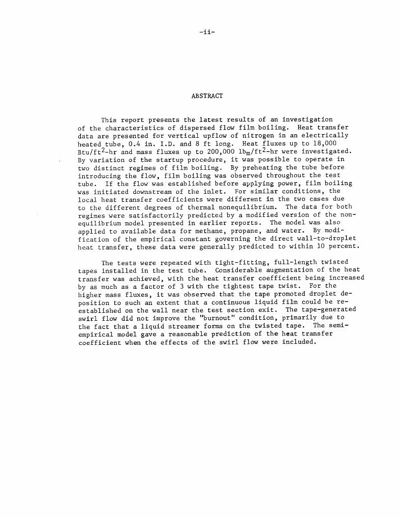
ABSTRACT

This report presents the latest results of an investigation

of the characteristics of dispersed flow film boiling. Heat transfer

data are presented for vertical upflow of nitrogen in an electrically

heated tube, 0.4 in. I.D. and 8 ft long. Heat fluxes up to 18,000

Btu/ft 2-hr and mass fluxes up to 200,000 lbm/ft 2-hr were investigated.

By variation of the startup procedure, it was possible to operate in

two distinct regimes of film boiling. By preheating the tube before

introducing the flow, film boiling was observed throughout the test

tube. If the flow was established before applying power, film boiling

was initiated downstream of the inlet. For similar conditions, the

local heat transfer coefficients were different in the two cases due

to the different degrees of thermal nonequilibrium. The data for both

regimes were satisfactorily predicted by a modified version of the non-equilibrium model presented in earlier reports. The model was also

applied to available data for methane, propane, and water. By modi-

fication of the empirical constant governing the direct wall-to-droplet

heat transfer, these data were generally predicted to within 10 percent.

The tests were repeated with tight-fitting, full-length twisted

tapes installed in the test tube. Considerable augmentation of the heat

transfer was achieved, with the heat transfer coefficient being increased

by as much as a factor of 3 with the tightest tape twist. For the

higher mass fluxes, it was observed that the tape promoted droplet de-

position to such an extent that a continuous liquid film could be re-

established on the wall near the test section exit. The tape-generated

swirl flow did not improve the "burnout" condition, primarily due to

the fact that a liquid streamer forms on the twisted tape. The semi-

empirical model gave a reasonable prediction of the heat transfer

coefficient when the effects of the swirl flow were included.

-iii-

ACKNOWLEDGMENTS

Financial support for this investigation was provided by the

National Science Foundation under Grant GK 1759. Professor P.

Griffith, Professor A. R. Rogowski, and Professor B. B. Mikic gave

generously of their time to discuss various aspects of this work.

Assistance in the experimental program was provided by Mr. W. D.

Fuller and Mr. E. D. Fedorovitch. Mr. F. Johnson was project

mechanic. Calculations were performed on the IBM 360 at the M.I.T.

Computation Center and on the IBM 1130 at the Department of Mechanical

Engineering Computation Center.

-iv-

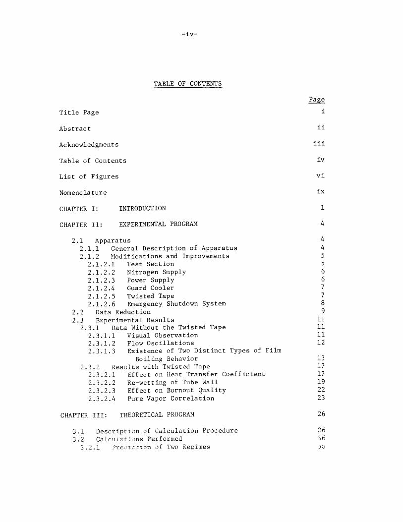
TABLE OF CONTENTS

Page

Title Page

Abstract ii

Acknowledgments iii

Table of Contents iv

List of Figures vi

Nomenclature ix

CHAPTER I: INTRODUCTION 1

CHAPTER II: EXPERIMENTAL PROGRAM 4

2.1 Apparatus 4

2.1.1 General Description of Apparatus 4

2.1.2 Modifications and Improvements 5

2.1.2.1 Test Section 5

2.1.2.2 Nitrogen Supply 6

2.1.2.3 Power Supply 6

2.1.2.4 Guard Cooler 7

2.1.2.5 Twisted Tape 7

2.1.2.6 Emergency Shutdown System 8

2.2 Data Reduction 9

2.3 Experimental Results 11

2.3.1 Data Without the Twisted Tape 11

2.3.1.1 Visual Observation 11

2.3.1.2 Flow Oscillations 12

2.3.1.3 Existence of Two Distinct Types of Film

Boiling Behavior 13

2.3.2 Results with Twisted TCape 17

2.3.2.1 Effect on Heat Transfer Coefficient 17

2.3.2.2 Re-wetting of Tube Wall 192.3.2.3 Effect on Burnout Quality 22

2.3.2.4 Pure Vapor Correlation 23

CHAPTER III: THEORETICAL PROGRAM 26

3.1 Descript'Lon of Calculation Procedure 26

3.2 Galcifl1-t2ons Performed 36 t

3.2.1 _?redic -on ot: Two Reglimes

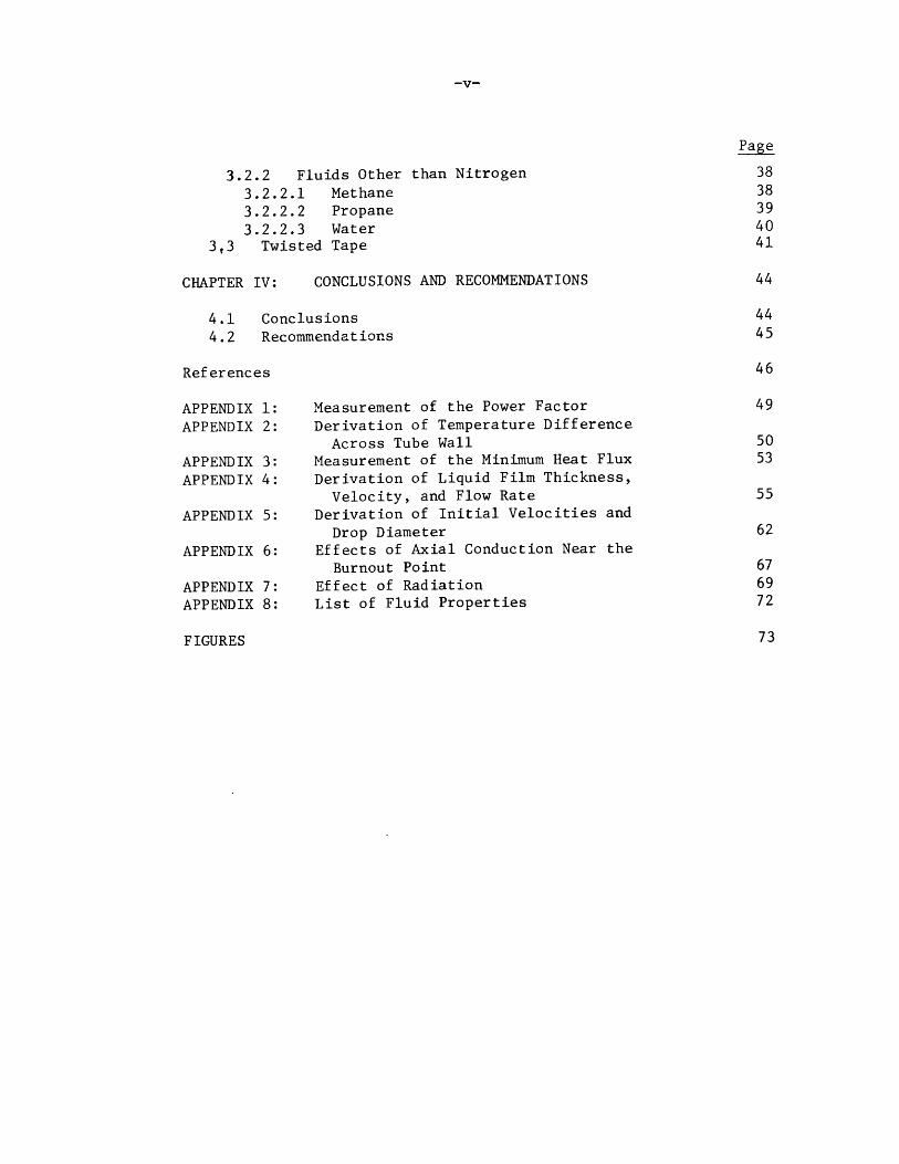
3.2.2 Fluids Other than Nitrogen

3.2.2.1 Methane3.2.2.2 Propane3.2.2.3 Water

3,3 Twisted Tape

CHAPTER IV: CONCLUSIONS AND RECOMMENDATIONS

4.1 Conclusions4.2 Recommendations

References

APPENDIX 1:APPENDIX 2:


APPENDIX 5:

APPENDIX 6:


Measurement of the Power Factor

Derivation of Temperature DifferenceAcross Tube Wall

Measurement of the Minimum Heat Flux

Derivation of Liquid Film Thickness,Velocity, and Flow Rate

Derivation of Initial Velocities and

Drop DiameterEffects of Axial Conduction Near the

Burnout PointEffect of RadiationList of Fluid Properties

FIGURES

Page

3838394041

-vi-

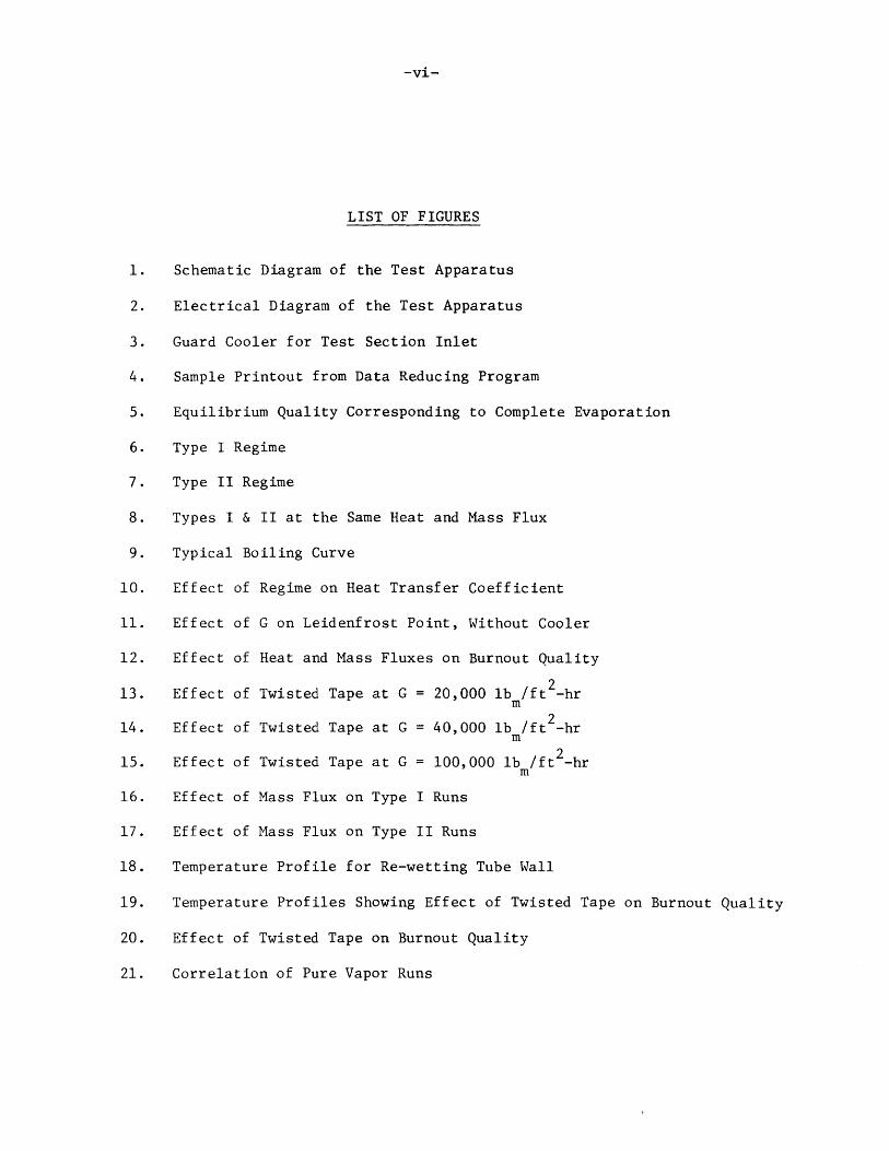
LIST OF FIGURES

1. Schematic Diagram of the Test Apparatus

2. Electrical Diagram of the Test Apparatus

3. Guard Cooler for Test Section Inlet

4. Sample Printout from Data Reducing Program

5. Equilibrium Quality Corresponding to Complete Evaporation

6. Type I Regime

7. Type II Regime

8. Types I & II at the Same Heat and Mass Flux

9. Typical Boiling Curve

10. Effect of Regime on Heat Transfer Coefficient

11. Effect of G on Leidenfrost Point, Without Cooler

12. Effect of Heat and Mass Fluxes on Burnout Quality

213. Effect of Twisted Tape at G = 20,000 lb /ft -hr

m14. Effect of Twisted Tape at G = 40,000 lb I ft -_hr

15. Effect of Twisted Tape at G = 100,000 lb /ft -hrm

16. Effect of Mass Flux on Type I Runs

17. Effect of Mass Flux on Type II Runs

18. Temperature Profile for Re-wetting Tube Wall

19. Temperature Profiles Showing Effect of Twisted Tape on Burnout Quality

20. Effect of Twisted Tape on Burnout Quality

21. Correlation of Pure Vapor Runs

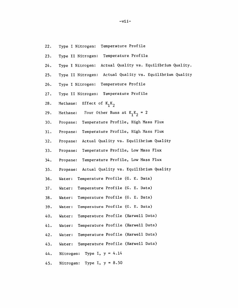
-vii-

22. Type I Nitrogen: Temperature Profile

23. Type II Nitrogen: Temperature Profile

24. Type I Nitrogen: Actual Quality vs. Equilibrium Quality.

25. Type II Nitrogen: Actual Quality vs. Equilibrium Quality

26. Type I Nitrogen: Temperature Profile

27. Type II Nitrogen: Temperature Profile

28. Methane: Effect of K K2

29. Methane: Four Other Runs at K1K2 = 2

30. Propane: Temperature Profile, High Mass Flux

31. Propane: Temperature Profile, High Mass Flux

32. Propane: Actual Quality vs. Equilibrium Quality

33. Propane: Temperature Profile, Low Mass Flux

34. Propane: Temperature Profile, Low Mass Flux

35. Propane: Actual Quality vs. Equilibrium Quality

36. Water: Temperature Profile (G. E. Data)




40. Water: Temperature Profile (Harwell Data)




44. Nitrogen: Type I, y = 4.14

45. Nitrogen: Type I, y = 8.50

-viii-

46. Nitrogen: Type II, y = 4.14

47. Nitrogen: Type II, y = 8.50

48. Power Factor vs. Voltage Across Test SectionV

49. Paths of Conduction at Test Section Inlet

50. Profile of Liquid Streamer

51. Void Fraction vs. Quality

52. Velocity Iteration

53. Boundary Conditions for the Axial Conduction Problem

54. Effects of Axial Conduction at Burnout Point

-ix-

NOMENCLATURE

acceleration, ft/hr 2

a0 centrifugal acceleration, ft/hr2

current, amps

flow area, ft2

cross-sectional area of liquid streamer, ft2

A v flow area taken up by vapor, ft2

0 coefficient of drag

C0 constant in heat transfer coefficient correlation

specific heat of vapor at constant pressure, Btu/lb -*FV m

diameter of tube, f t2

Fanning friction factor

F fraction of heat lost through outer wall of tube

acceleration of gravity = 4.17 x 108 ft/hr2

mass flux or mass velocity, lbrm/ft -hr

- Grashof number

latent heat of evaporation, Btu/lbm

h latent heat of evaporation plus superheat, Btu/lbm

A latent heat of evaporation, corrected (Baumeister et al.),

Btu/lbm

heat transfer coefficient from vapor to droplet, Btu/ft 2-hr-*F

heat transfer coefficient from wall to droplet, Btu/ft -hr-*F

2h heat transfer coefficient from wall to vapor, Btu/ft -hr-*F

K thermal conductivity, Btu/ft-hr-*F

tape curvature, ft 1

T Tthermal conductivity of vapor, evaluated at v + w

Btu/ ft-hr-*F

empirical constant relating to gravity

/2 empirical constant relating to packing

empirical constant relating to streamer width

empirical constant relating to friction factor

length of tube, f t

/2 exponent in heat transfer coefficient correlation

N/Z number of drops per unit surface area, ft2

A/ number of drops per unit volume, ft3

A/, Nusselt number

pressure, psia

power, watts

1r Prandtl number

(?/A4 heat flux, Btu/ft -hr

' radius, ft

/; inner radius of tube, f t

r6 outer radius of tube, f t

R half-width of liquid streamer, ft

9&e Reynolds number

Res Reynolds number for droplet

,Qe hydraulic Reynolds number

-xi-

thickness of liquid streamer, ft

average thickness of liquid streamer, ft

vapor temperature, *R or *F

7 saturation temperature, *R or *F

// wall temperature, *R or *F

emf across test section, volts

\/, average axial velocity of liquid streamer, ft/hr

VI average axial velocity of droplets, ft/hr

\/V average axial velocity of vapor, ft/hr

V-2 axial velocity of liquid streamer, ft/hr

L V difference in velocities, defined at each use, ft/hr

\A/ heat generation per unit volume, Btu/hr-ft3

We Weber number

\Ae, critical Weber number

mass flow rate of liquid streamer, lb m/hr

64Av mass flow rate of vapor, lb m/hr

actual quality

equilibrium quality

X0 actual quality at point of last shattering

length of tape for 180* twist/tube diameter

axial position or dimension, ft

void fraction

measure of tape twist = ff/2y

&i droplet diameter, ft

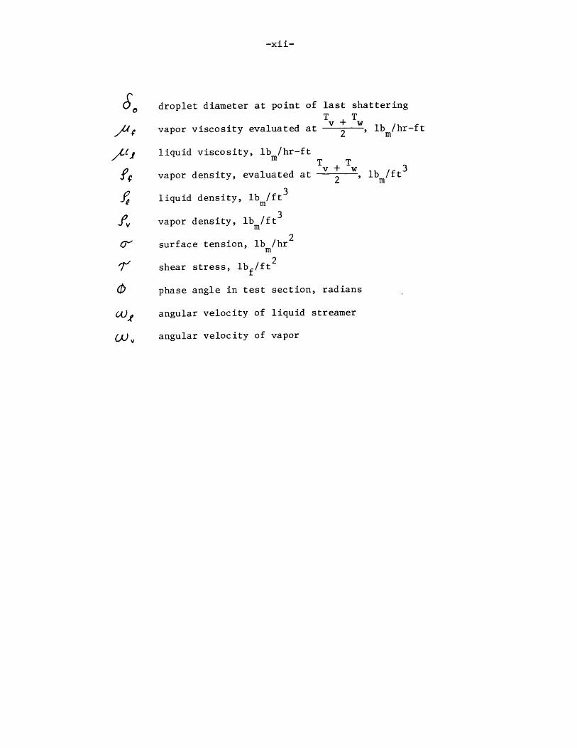
-xii-

droplet diameter at point of last shatteringT T

vapor viscosity evaluated at v + W lb /hr-ft2 m

7Lttj liquid viscosity, lbm/hr-ftm T +T lbft

vapor density, evaluated at 2 ,lbm/ft

liquid density, lb/ft 3

vapor density, lbm/ft 3

surface tension, lb m/hr2

shear stress, lb f/ft 2

phase angle in test section, radians

4) angular velocity of liquid streamer

(A) angular velocity of vapor

-1-

INTRODUCTION

Forced convection dispersed flow film boiling is of more than aca-

demic interest. It occurs in once-through steam generators and in

cryogenic transfer lines as well as in nuclear reactor cores and steam

generators that have undergone loss-of-coolant flow accidents. It is

important to be able to predict the tube wall temperatures involved in

film boiling, since the temperatures are often close to or exceeding

the melting point of the tube material.

Dispersed flow occurs under quality conditions and is charac-

terized by liquid droplets entrained in a vapor flow. Dispersed flow

film boiling generally involves thermodynamic non-equilibrium. Due to

a lack of continuous direct contact between liquid and heated surface,

the dominant path of heat transfer is from tube wall to vapor, thence

from vapor to drop. Some heat is transferred directly from tube wall

to droplet, but this is important only at low qualities. The fact

that this process is not instantaneous means that the entrained drops

(or droplets; the terms are used interchangeably) are carried past the

point where they would have boiled under equilibrium conditions. This

permits superheated vapor. A sizeable discrepancy often exists between

equilibrium quality (as determined by the first law of thermodynamics)

and actual quality (the flowing mass fraction of fluid that has evapora-

ted); the actual quality may be as low as 60% of the equilibrium quality.

-2-

This report is one of a series of reports resulting from the Film

Boiling Project at the MIT Heat Transfer Laboratory. The goal of this

project is to better predict the behavior of forced convection film

boiling by means of better understanding its mechanisms. Early work on

this project by Kruger(1 ) and by Dougall(2) used Freon - 113 as the

experimental fluid. This work was limited to low qualities, partly be-

cause Freon - 113 was observed to decompose at the temperatures associ-

ated with film boiling. Laverty introduced the use of liquid

nitrogen as the experimental fluid because it does not decompose and

because it can film boil at temperatures below room temperature, and

developed a procedure for calculating actual qualities and tube wall

temperatures based on a model of heat transfer from wall to vapor and

from vapor to drop. Forslund(5, 6) measured the extent of the non-

equilibrium by measuring actual vapor qualities; he also introduced a

term describing the heat transferred directly from wall to droplet

into the calculation procedure. By the use of two empirical constants,

he arranged to fit the theory to the nitrogen data that he took.

It was the purpose of this work to take data under a wider range of

conditions than those of Forslund and to see if his model would fit the

data without having to change the empirical constants, and to see if the

model could predict the data of other experimenters using other fluids.

A second goal was to investigate the effect of a twisted tape inserted

into the test section, of which the purpose was to augment the heat

transfer coefficient (particularly the wall to droplet portion) by

Numbers in parentheses refer to references, found on p. 46.

-3-

centrifuging the drops against the heated wall. Finally, the model

was to be adapted to this more complex geometry.

-4-

EXPERIMENTAL PROGRAM

2.1 Apparatus

The experimental apparatus was originally built by Laverty, modified

by Forslund, and further modified by the author.

2.1.1. General Description of Apparatus:

A schematic diagram of the system is given in Figure 1. Liquid

nitrogen at 106 psia is allowed to flow through two heat exchangers

that cool it down sufficiently that it remains liquid as it passes

through the flow control valve. The subcooling is achieved by bleeding

part of the main flow into a vacuum line, which forms the outer part

of the two concentric-tube heat exchangers. The nitrogen enters the

test section at about 20 psia.

In the vertical test section, the pressure is monitored by five

pressure taps in conjunction with a manometer board. Tube wall tempera-

tures are measured at 24 points by copper-constantan thermocouples that

are spot-welded to the outer tube wall. The tubular test section is

direct resistance heated by a power supply described by Figure 2 and

is insulated on its outer surface by a jacket containing 1-1/2 inches

of Santocel, a finely powdered silica.

-5-

The nitrogen then passes through a visual test section consisting

of a glass tube with an electrically conducting coating on the outside.

Current is passed through the coating to heat the tube to keep it from

frosting up. The nitrogen then passes through one or two concentric-tube

heat exchangers which serve to heat up or cool down the nitrogen to

roughly room temperature before it goes through the rotameters. The

steam or water that flows through the outer part of these heat exchangers

also flows through another heat exchanger that heats up the vacuum line

so that the vacuum pump does not freeze up.

Further description of the apparatus can be found in references

5 and 7.

2.1.2. Modifications and Improvements:

2.1.2.1. Test Section

The test section for the majority of the tests was made of Inconel

600 supplied by Whitehead Metals Company instead of stainless steel as

was used by previous investigators (however, Forslund's 0.228" stainless

steel test section was used for the tests reported in section 2.3.1.1.).

The electrical resistivity of Inconel varies by about 4% over the

range of 600*R to 1700*R; this change is small enough to permit the

assumption that the heat generation is constant along the entire length

of the tube, even in the presence of large temperature gradients. The

dimensions of the test section were: length = 8 ft, I. D. = 0.400 in.,

0. D. = 0.500 in.

-6-

2.1.2.2. Nitrogen Supply

The 50 liter Dewar flask used by Laverty and Forslund was replaced

by a 160 liter Dewar (Linde LS-160). Besides the obvious advantage of

less frequent replacement, the 160 liter Dewar could withstand pressures

up to 150 psi. To achieve high pressures, the standard 22 psig relief

valve was replaced by a 100 psig valve. High pressures were deemed use-

ful because it was felt that one type of flow oscillation could be

avoided by severe throttling at the test section inlet, and a high pres-

sure permits such throttling. During operation, flow oscillations were

observed, particularly during start-up. They were described to other

causes, as detailed in section 2.3.1.2. Higher pressures and larger

nitrogen capacity also permitted operation at higher mass fluxes.

2.1.2.3. Power Supply

The use of two ganged,variable transformers and two stepdown trans-

formers in parallel, as shown in Figure 2, permitted heat fluxes up to

18,000 Btu/ft -hr. Forslund achieved higher heat fluxes (up to 23,000

Btu/ft -hr, averaged along the length of the test section) but by using

tubes of smaller diameters (0.228 in. and 0.323 in.).

The power factor was measured (see Appendix 1) and found to be 0.94.

The increased current made it necessary to install a current transformer

as shown in Figure 2. This transformer has more than one secondary tap;

-7-

the tap with the 80:1 ratio was used. This transformer, Weston Model

401, Type 2, has a nickel alloy core with a low phase angle for use with

wattmeters; thus, it was suitable for measuring the power factor.

2.1.2.4. Guard Cooler

For some of the experiments it was necessary to prevent heat from

leaking in through the power lead at the inlet of the test section. To

effect this, the guard cooler shown in Figure 3 was bolted into the

power line roughly six inches away from the test section inlet and the

power line was well wrapped with fiber glass insulation. The two flare

fittings permitted the cooler to be connected, in series, into the

vacuum line between the transfer tube heat exchanger and the bleed back

pressure control valve. In practice, it cooled down the line so well

that heat conduction away from the test section became something of a

problem. Unfortunately, it could not be controlled, as the vacuum line

could not be throttled and still have the heat exchangers prevent flash-

ing at the flow control valve.

2.1.2.5. Twisted Tape

A twisted strip of Inconel 600, 0.400 in. x 0.020 in. x 8 ft., was

inserted in the test section and secured at the upstream end by silver

soldering.

-8-

The purpose of the tape was to centrifuge the droplets onto the

tube wall so as to hasten their evaporation and to cool the wall.

After data were taken with the twist ratio y (defined as the number of

tube diameters per 180* of twist) equal to 8.5, the tape was removed,

twisted again to a twist ratio of 4.1, and reinserted. As the tape

was designed to fit tightly inside the tube, insertion involved lubri-

cation with oil and subsequent flushing with solvents.

The twist ratio was not perfectly uniform along the length of the

tape. Indeed, for the twist ratio reported as 8.5, the local twist

ratio varied from 7.0 to 10.0, with three maxima and four minima regu-

larly spaced along the tape. This was thought to be due to the fact

that the tape was made up of four 2' sections welded together; the three

maxima in twist ratios (i.e., least twisted portions) occurred in the

vicinity of these welds. These welds were necessary because the longest

sheet of Inconel 600 available to us was two feet long.

2.1.2.6. Emergency Shutdown System

The emergency shutdown system was modified to include a normally-

closed solenoid valve in the liquid delivery line connected across the

primary of one of the variable transformers, as shown in Figure 2. Thus,

one emergency switch could shut off the power and the flow. A small

variable transformer was installed in the solenoid valve circuit, since

the other 75% of the power would have been dissipated into the delivery

line because the solenoid valve as well as the delivery line was wrapped

-9-

in fiber glass insulation. This heat generation would have prevented

the attainment of reasonable inlet subcooling, or could have even

caused boiling in the delivery line.

2.2. Data Reduction

The data were reduced by a computer program, a sample printout of

which is shown in Figure 4. This program calculates heat flux from

voltage and current readings, and mass flux from flowmeter (Rotameter)

readings. As a check for error, the latter readings are also printed

out. Note that the current readings are those in the secondary circuit

of the current transformer; the test section current is 80 times this.

The five manometer readings are converted to five pressures at

the pressure taps, from which a fourth-order curve fit to the pressure

along the test section is made. This curve fit is evaluated at each of

the 24 points along the test section at which there is a thermocouple.

From the pressure are calculated the pressure gradient and the saturation

temperature.

From the inlet temperature is calculated the inlet subcooling.

This allows calculation of the equilibrium quality at the 24 points.

The bulk temperature, which assumes equilibrium conditions, is set

equal to the saturation temperature for equilibrium qualities between

zero and one; for equilibrium qualities less than zero or greater than

one, the bulk temperature is modified by the specific heat of the

liquid and vapor,respectively.

-10-

The thermocouple readings are converted to outer wall temperatures

by means of a subroutine which is a collection of eleven fourth-order

curve fits to the thermocouple tables, each spanning a different portion

of the tables. The inner wall temperatures are calculated by means of

an equation derived in Appendix 2. The temperature drop across the

tube wall was never more than 5*F, and was usually much less.

The equilibrium heat transfer coefficient is then calculated,

based on the bulk temperature and the inside wall temperature and on

the average (assumed uniform) heat flux. This heat flux was simply

the heat generated divided by the inside tube area. It was not modified

to account for end conduction, for with the exception of the tests de-

scribed in section 2.3.1.3. (for which end conduction was treated in

Appendix 3), the area of interest was not near either end. The formula

for heat flux was not modified for the tests with the twisted tape,

either. Although 10% of the heat was generated in the tape (based on

the observed change of the test section resistance when the tape was

installed), its area was sufficiently large that heat flux from the tape

was quite small. The fin efficiency of the tape was calculated by

Lopina(8) and found to be small enough that the tape could be ignored

as a heated surface. This does admit some error;but the error is les-

sened by the fact that both the data reduction program and the analyti-

cal model program use the same assumption.

The reduced data for over 200 runs are on file in the MIT Heat

Transfer Laboratory.

-11-

2.3. Experimental Results

2.3.1. Data Without the Twisted Tape:

2.3.1.1. Visual Observations

The increased mass flux possible with the large Dewar permitted the

confirmation of a trend observed by Forslund. The existence of thermo-

dynamic non-equilibrium is easily and demonstrably observed by the viewing

of droplets in the visual test section at exit qualities greater than one.

Forslund observed that the equilibrium quality at which droplets disappear

is much greater at low mass fluxes than at high mass fluxes. This is an

indication that non-equilibrium decreased with increasing mass flux.

To achieve high mass fluxes, Forslund's 0.228 in, diameter, 8 ft.

long test section was used. These were the only tests for which this

test section was used. The method of looking for drops was to aim a

strobe light into the visual test section and to try to "stop" their

motion. It was often observed, generally near the point of marginal

visibility of drops, that they seemed to appear in bursts, or clusters.

The existence of drops was only one of several factors entering into

their visibility. Others were the angle of the incident light and even

the amount of time spent looking for drops. Liquid nitrogen drops are

colorless, fast-moving, and easily overlooked when present and imagined

when not under conditions of poor visibility. It is difficult to esti-

mate the size of the smallest drops observed, for drops of almost any

"Mawfte-

-12-

size will scatter light. Our data (the filled-in circles of Figure 5)

confirm the trend of Forslund's data.

2.3.1.2. Flow Oscillations

Despite the severe throttling at the test section inlet, flow

oscillations of several types were encountered. The first, and most

easily explained, was that which occurred during startup. As the inlet

plumbing was cooled down by the nitrogen flowing through it, liquid

began to replace the vapor flowing through the flow control valve. As

a slug of liquid passed through, the pressure drop across the valve

decreased markedly, causing a sudden flow increase until the liquid

slug had passed entirely through. Once the flow through the valve

became entirely liquid, the valve could be closed down some and the

flow would become constant.

Under all running conditions, small pressure fluctuations typical

of two phase flow were present. As they affected the manometers just

enough to render readings difficult, throttling orifices were put in

the manometer lines which slowed the response time of the manometers

from the order of a tenth of a second to the order of a second. Flow

oscillations with a period larger than about a second were still ob-

servable.

One type of flow oscillation that was not so easily explained was

the sort that occurred in the early runs whenever the ratio of mass

-13-

flux to heat flux fell below 4.0 (lbm/Btu). This was not observed with

the stainless steel test section, nor with the twisted tape installed.

Flow oscillations of perhaps another type were preceded by considerable

pressure changes in the bleed flow line. These were thought to be due

to flashing in the delivery line or freezing in the bleed line, as

conditions in the bleed line were near the triple point.

A complete explanation of the observed flow oscillations is not

the goal of this thesis; these observations are reported merely for

their value as observations. It should be noted that no flow oscil-

lations (except, of course, the small fluctuations that were masked by

the throttling orifices) were present in any of the data runs reported

in this thesis.

2.3.1.3. Existence of Two Distinct Types of Film Boiling Behavior

Two distinctly different regimes of film boiling were observed.

The first, shown qualitatively in Figure 6 (an actual example is shown

in Figure 22), was the same kind observed by Laverty and Forslund. The

entire test section is in film boiling, the burnout point being essen-

tially at the entrance to the test section. The second, shown quali-

tatively in Figure 7 (an actual example is shown in Figure 23), has

nucleate boiling and an annular dispersed region before the burnout

point. The wall temperature in the annular region was noticeably

lower than that in the nucleate boiling region.

-14-

The term "burnout" is not used here in its usual sense, as the

phonomenon it describes occurs at low enough temperatures with nitro-

gen that the tube is in no danger of melting. Indeed, this is why

nitrogen was chosen as the experimental fluid.

Both regimes can occur at a given heat flux and mass flux, as

evidenced by Figure 8. Which regime will occur is determined by the

manner in which the test conditions are achieved. If the tube is

allowed to heat up before flow is begun and if the entrance of the

test section is always kept at a temperature above the Leidenfrost

temperature, then a Type I regime will occur. Figure 9, a sketch of

the boiling curve, provides a good definition of the Leidenfrost

point. If the temperature of the test section entrance is cooled be-

low the Leidenfrost temperature, such as by letting liquid nitrogen

flow through it before the power is turned on, then a Type II regime

will occur. Both regimes were also observed to occur with the twisted

tape installed.

The two regimes have different degrees of thermodynamic non-

equilibrium, even at the same heat and mass flux, which results in

different tube wall temperatures. Type I regimes, with burnout at

the entrance, build up non-equilibrium from the entrance, whereas

Type II regimes are in equilibrium upstream of the burnout point

(superheated vapor cannot exist inside a liquid film at saturation

temperature). The greater the discrepancy between actual and equilib-

rium qualities, the greater the vapor superheat, according to the first

-15-

law of thermodynamics.

XE f= X -- YA F f9--cpv v-T (2-1)

Thus, at a given equilibrium quality, a Type I run will have a lower

actual quality, thus a higher vapor temperature and a higher wall

temperature than will a Type II run with the same heat and mass fluxes.

Figure 10 shows this for a collection of early runs.

Transition from Type I to Type II, but not from Type II to Type

I, is possible by changing the heat flux. Once the heat flux is dropped

below that value corresponding to the Leidenfrost point, a liquid film

will appear at the beginning of the test section and will in some cases

move up the test section, asymptotically approaching some equilibrium

point. When operating in the Type II regime, however, increasing the

heat flux past the Leidenfrost point merely causes the liquid film to

recede; no doubt there is some heat flux at which the Type II to Type

I transition will occur, but it is beyond the capability of our appa-

ratus.

The heat flux at which the Type I to Type II transition occurred

was measured for several different mass fluxes in an effort to deter-

.mine what effect mass flux had on the Leidenfrost point. As Figure 11

will attest, the change is small and vague. On the theory that con-

duction into the test section through the power line could be present

in sufficient degree to mask the observation of such a trend, the

-16-

guard cooler of Figure 3 was installed to halt (or, as it turned out,

to reverse) this conduction. Measurement of the heat flux below which

transition occurred (or minimum heat flux) was made difficult because

sufficient heat was conducted from the test section to the cooler so

that the full capacity of electrical power was needed to maintain a

Type I regime. Measurement of this minimum heat flux was impossible

at more than one mass flux; increasing the mass flux caused transition

(this did indicate that the minimum heat flux does increase with in-

creasing mass flux), and decreasing the mass flux would have resulted

in dangerously high temperatures at the downstream end of the test

section. As it was, at the one mass flux at which the minimum heat

flux was determined, the last six inches (which had become uncovered

by the insulation) was glowing red and estimated to be at 1400*F and

all the thermocouples except those in the first two inches of the test

section were off the scale of the recorder, which corresponded to

temperatures greater than 700*F.

In Appendix 3, the heat flux at the Leidenfrost point was deter-

2 2mined to be 2,200 Btu/ft -hr at a mass flux of 40,000 lb /ft -hr underm

conditions of conduction into the test section inlet through the

power line and 18,700 Btu/ft -hr at the same mass flux under conditions

of conduction away from the test section. This conduction at the test

section ends can explain the discrepancy between the data and the pre-

dictions of the model developed in the next chapter that occurred at

the thermocouple nearest each end of the test section# because the

model didn't take into account axial conduction.

-17-

Type I film boiling is the regime that occurs in a cryogenic

transfer line when flow of a cryogenic liquid is first introduced into

a warm line. Transition from Type I to Type II occurs after the first

portion of the tube has cooled below the Leidenfrost point. Type II

film boiling is the regime that exists after burnout in a boiler tube.

The equilibrium quality at burnout for the Type II runs was ob-

served to decrease with increasing heat flux and to increase with in-

creasing mass flux, as indicated by Figure 12.

2.3.2. Results with Twisted Tape:

2.3.2.1. Effect on Heat Transfer Coefficient

The twisted tape was effective in raising the heat transfer

coefficient at all values of heat flux and mass flux, as shown in

Figures 13, 14, and 15. The tighter tape twist was more effective.

The next section will explain why the dashed lines of Figure 15 go

off scale. It is interesting to note that in Figure 13, some of

the lines are observed to cross, indicating that at low qualities

and low mass fluxes, the heat transfer coefficient decreases with

increasing mass flux; the opposite is generally the case, as evidenced

by Figures 14 and 15 and the high quality portion of Figure 13. This

phenomenon is due to the direct heat transfer from wall to droplet,

which becomes most noticeable under the conditions of low quality and

mass flux. At low quality, droplets are numerous, whereas at high

-18-

quality, droplets are scarce. As will be pointed out in the next

chapter, the heat transfer coefficient for the wall to droplet

term is relatively insensitive to mass flux, whereas the wall to vapor

term is proportional to mass flux. The heat transfer coefficient at

the wall, defined by

(A) (2-2)W~ a-t

is the sum of a convective (wall to vapor) term and a direct (wall to

droplet) term.

(2-3)

For the reasons given above, the direct term is dominant under these

circumstances. As will be shown more exactly in the next chapter,

w, (2-4)

The exponent is not exactly - 1/3, nor is it constant, but this is a

good rough idea. Thus, neglecting the convective term of equation( 2-3 )

Comparing equations (2-4) and (2-5) , it is seen that

(2-6)

-19-

Thus, at low mass flux and low quality (as is the case for the left-

hand portion of Figure 13), the heat transfer coefficient should in-

crease with decreasing heat flux, as is evidenced by the crossing of

the lines on Figure 13.

The pressure drop across the test section was also observed to

increase as well; this effect and its significance in view of the in-

creased heat transfer coefficient are dealt with in detail by Fuller, (7)

who concluded that for a tube-temperature-limited system, the increased

heat transfer coefficient allows considerably shorter tubes with no in-

crease in pressure drop.

Figures 16 and 17 show the effect of mass flux and illustrate the

fact that both regimes can exist with the twisted tape. The similarity

of curves of each family would indicate the possibility of a correla-

tion; however, this was not the purpose of this work.

2.3.2.2. Re-wetting of Tube Wall

For high values of mass flux the act of decreasing the heat flux

below a fairly definite point resulted in the establishment of a liquid

film after a section of film boiling. The heat transfer coefficient

increases to values typical of nucleate boiling, as indicated by the

dashed lines of Figure 15. A typical temperature profile is shown in

Figure 18. This was observed only with Type I regimes; however, no

particular effort was made to observe this phenomenon with Type II

regimes. Raising the heat flux again above this point results in the

disappearance of the film. Once the film does form on the wall, no

further decrease in power is necessary to allow it to spread in both

directions. This is because axial conduction along the test section

-20-

toward the portion with the liquid film cools the adjacent portion,

thus decreasing the force repelling the drops from the wall until they

too contact and wet it. The film was not allowed to expand until it

stabilized, if indeed it ever would have. The expansion was slow, the

phenomenon occurred only at high mass fluxes, and it appeared that we

would run out of nitrogen before expansion ceased.

Listed below are the pertinent operating conditions and resulting

temperatures at a heat flux barely above that which made the re-wetting

occur.

Run Mass Flux Heat Flux wall sat Quality y

No. lb /ft -hr Btu/ft -hr OR *Rm

221 100,000 9,400 312 146 .909 4.14

158 84,000 4,300 265 144 .549 8.50

160 85,000 4,500 259 144 .545 8.50

166 133,000 10,100 288 146 .806 8.50

168 132,000 10,000 293 145 .840 8.50

173 185,000 15,600 305 147 .895 8.50

These data represent conditions under which the centrifugal

force on the droplet is just enough to overcome the Leidenfrost

force (that force, due to rapid vapor generation between the

drop and the heated surface, which repels the drop from the surface)

and to allow the drops to touch (and presumably to wet) the wall.

The very high heat transfer coefficient that results indicates

that the wall is completely re-wetted. These data, particularly

when coupled with calculations of the droplet's diameter made possible

-21-

by the procedure outlined in the next chapter, form a basis for evalua-

tion of any theoretical calculation of the Leidenfrost force.

It is worth noting that while the term 're-wetting' is used, this

phonomenon was observed only with Type I runs, where no liquid film

existed on the wall upstream of the point described by the above Table.

Two Type II runs with the twisted tape were taken with mass fluxes

comparable to those listed above. These are tabulated below.

Run Mass Flux Heat Flux Quality at y

No. lb /ft -hr Btu/ft -hr Burnoutm

241 104,000 8,500 0.768 4.14

242 101,000 12,200 0.740 4.14

Of these, only Run 241 had a heat flux comparable to the 're-wetting'

runs. The quality at burnout of Run 241 was almost as high as the

quality at which re-wetting occurred for Run 221, which suggests that

were the heat flux decreased further, the centrifuged droplets would

merely extend the existing film, rather than establish a new one. This

hypothesis is borne out both by Figure 12, which shows that burnout

quality increases as heat flux decreases; and by the fact that the

most easily wetted portion of the dry wall is the relatively cool

portion bordering the liquid film, as evidenced by the tendency of a

re-wetted film to expand, once formed, with no further decrease in

power.

-22-

2.3.2.3. Effect on Burnout Quality

When a Type II run with the twisted tape is compared with a Type

II run with the same heat and mass fluxes but without the twisted tape,

the former is seen to burn out upstream of the point at which the

latter burns out, and often at a lower equilibrium quality. See

Figure 19 for an example of two Type II runs with roughly the same

heat and mass fluxes. The apparent anomaly in the above statement

is due to the reduction in flow area caused by the presence of the

twisted tape.

Moeck et al.(32) observed a similar phenomenon with 1000 psig

water, namely that burnout heat flux was increased by the presence

of a twisted tape provided that the mass flux was greater than

2500,000 lb ft -hr. The opposite effect was observed for mass

m

fluxes smaller than 500,000 lb m/ft -hr. Figure 20 shows the effect

of heat and mass fluxes on the equilibrium quality at burnout, for

the nitrogen data of the present study, both with and without the

twisted tape. It is to be noted that the difference in burnout

qualities due to the tape is most pronounced in the high quality,

low heat flux portion of Figure 20. Two conflicting phenomena

enter into this result, and their relative intensities determine

its extent.

The first effect of the twisted tape is to set up a centrifugal

force field that tends to centrifuge the droplets toward the wall and

into the liquid film that covers the wall upstream of the burnout point.

This effect alone would cause the presence of the twisted tape to bring

about a higher burnout quality; for with more liquid on the wall, more

-23-

evaporation must take place before the film is thin enough to permit

burnout. Were this the only effect of the twisted tape, the result

would be as described in this paragraph and not as observed.

Another effect of the twisted tape, and an important one, is

that it provides an area on which a portion of the liquid can cling.

In the center of the tube, centrifugal force (assuming that the tape

produces essentially a solid body rotation) is zero. Near the center,

surface tension can hold together a streamer of liquid against the

small centrifugal force near the center. An attempt to calculate

the amount of liquid that could be contained on the tape by this

force balance is made in Appendix 4; the conclusion is that surface

tension can account for large amounts of liquid and that surface

tension is not the limiting factor.

The theory of a streamer running up the middle of the tape is

strengthened by the observation of droplets in the visual test section

at exit qualities greater than one with the tape installed. The main

function of the tape was originally to decrease the non-equilibrium.

2,3,2.4, Pure Vapor Correlation

In an effort to determine the validity of the conventional

correlation for single phase forced convection heat transfer to a

tube containing a twisted tape under conditions of a high ratio be-

tween the wall temperature and the fluid temperature, some pure vapor

runs were taken. Once the liquid in the Dewar was expended, the

pressurizing nitrogen flowed through the cold Dewar and delivery

-24-

line and reached the test section at a temperature only slightly

-above saturation. Data runs had to be taken quickly, as the inlet

temperature of the vapor rose steadily as the temperatures of the

Dewar and delivery line rose. The vapor temperature was calculated

at each point in the test section using the first law of thermodynamics,

based on the exit temperature. The use of the inlet temperature gave

very scattered results; this was assumed to be due to the fact that

the fluid was not quite pure vapor at the inlet, but that it had

some drops entrained in it, causing the inlet thermocouple to read

various temperatures between saturation temperature and the vapor

temperature. Neither heat flux nor mass flux was varied more than

10% as the object was to observe the effect of different temperature

ratios. The inlet vapor temperature increased from about 160*R to

about 250*R during the course of these four runs. After these four

runs were taken, the inlet temperature began rising too fast for all

24 wall temperatures to be read at essentially the same time as the

fluid temperature.

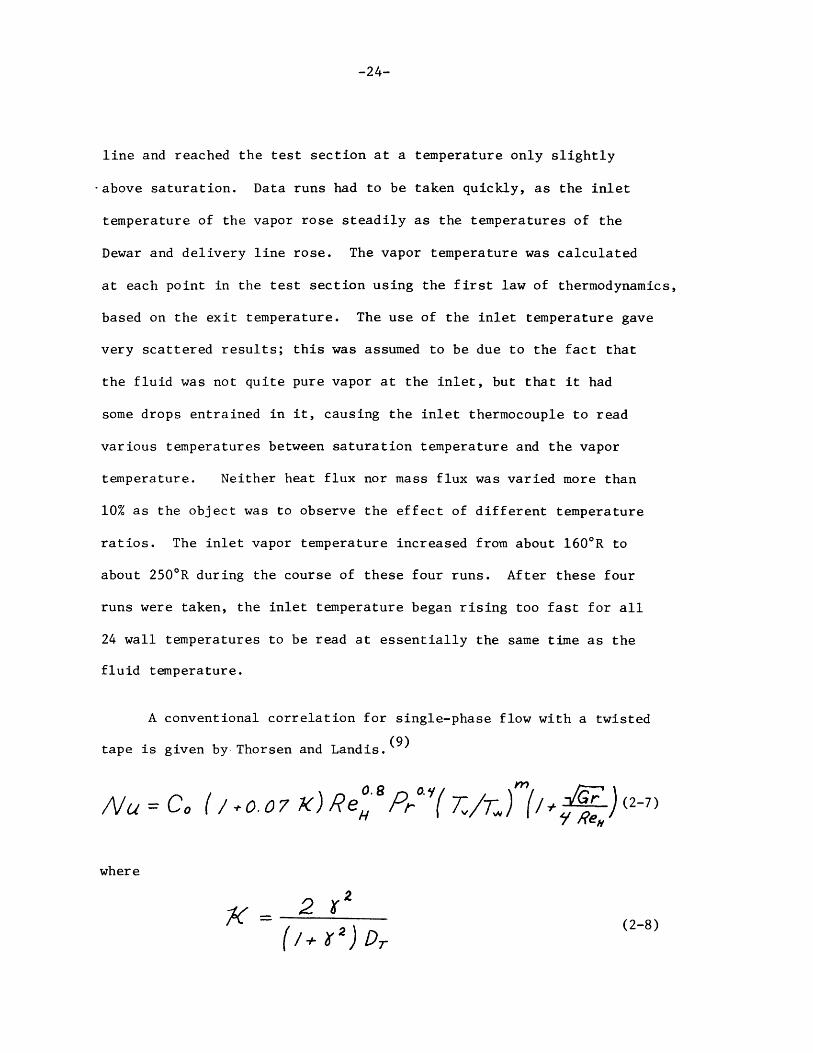
A conventional correlation for single-phase flow with a twisted

tape is given by Thorsen and Landis. 9 )

/\U = Co (/ 0.o0 7 k) Re 8 Pr-O( 7T )(/+ N (2-7)

where

(2-8)

(i+ 2) L)7

-25-

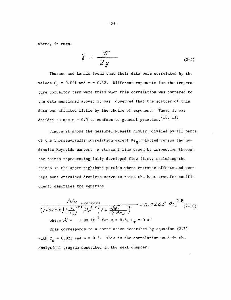
where, in turn,

/(2-9)

Thorsen and Landis found that their data were correlated by the

values C = 0.021 and m = 0.32. Different exponents for the tempera-

ture corrector term were tried when this correlation was compared to

the data mentioned above; it was observed that the scatter of this

data was affected little by the choice of exponent. Thus, it was

decided to use m = 0.5 to conform to general practice. (10, 11)

Figure 21 shows the measured Nusselt number, divided by all parts

of the Thorsen-Landis correlation except ReH, plotted versus the hy-

draulic Reynolds number. A straight line drawn by inspection through

the points representing fully developed flow (i.e., excluding the

points in the upper righthand portion where entrance effects and per-

haps some entrained droplets serve to raise the heat transfer coeffi-

cient) describes the equation

-=0.62&5 Re(/- .r7IV/+- q (2-10)

where K = 1.98 ft for y = 8.5, DT = 0.4"

This corresponds to a correlation described by equation (2.7)

with C = 0.023 and m = 0.5. This is the correlation used in the0

analytical program described in the next chapter.

-26-

THEORETICAL PROGRAM

3.1 Description of Calculation Procedure

The analytical program referred to earlier is similar to one

used by Forslund(5, 6) who extended the basic analysis proposed by

Laverty(3, 4). A fairly detailed description of the calculation

procedure is followed by a discussion of the assumptions made and

of the differences between this computer program and its predecessors.

The method of calculation is to determine vapor velocity,

droplet velocity and droplet size, at a point in the tube where

equilibrium conditions are assumed to exist, by iterating equations

(A5-16) and (A5-ll) of Appendix 5. The first of these equations is

one form of the continuity equation; the second is an expression of

the force balance between drag, gravity, and acceleration of the

drop, constrained by the critical Weber number criterion for deter-

mination of maximum drop size. These equations are solved by

iteration, as described in Appendix 5. The tube wall temperature

is calculated next by evaluating the wall-to-vapor heat transfer and

the wall-to-drop heat transfer, where it is assumed (for this initial

point only) that the vapor temperature is equal to the saturation

temperature (because equilibrium was assumed).

-27-

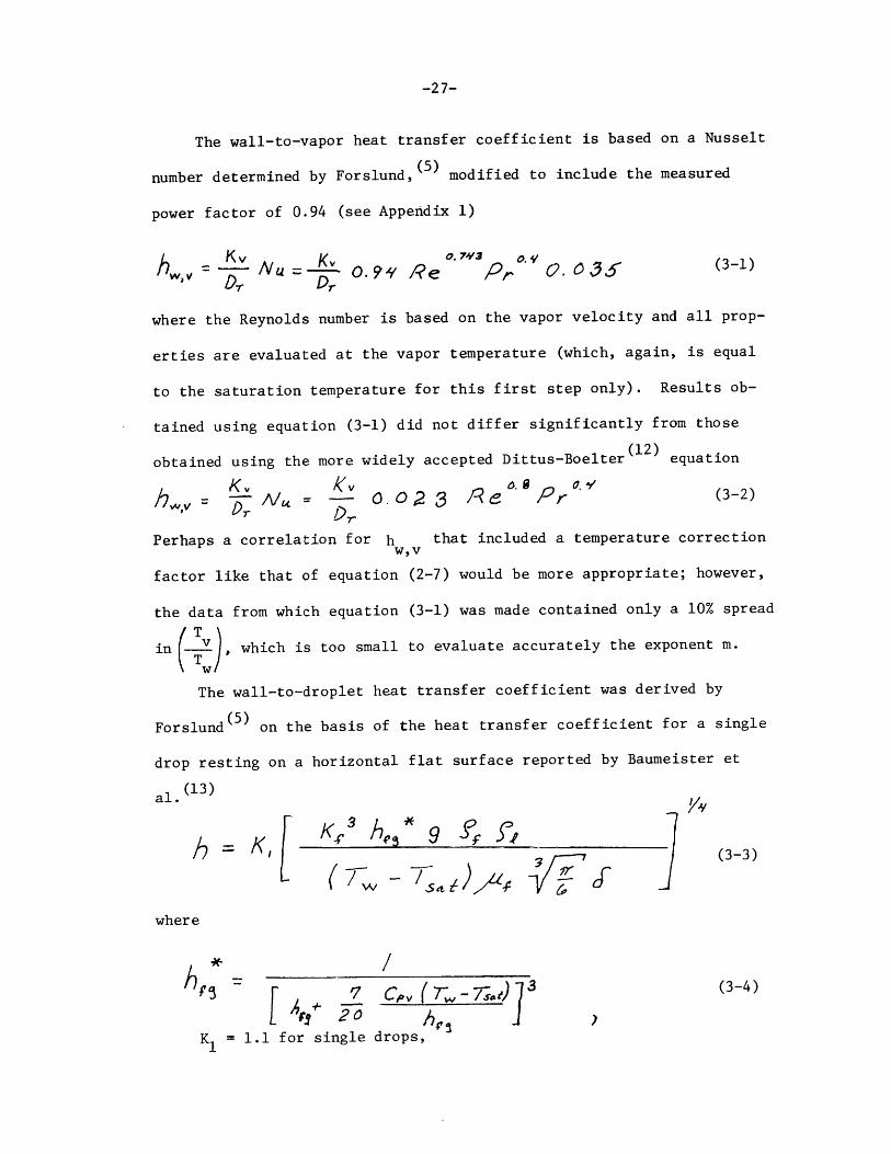
The wall-to-vapor heat transfer coefficient is based on a Nusselt

number determined by Forslund, (5) modified to include the measured

power factor of 0.94 (see Appendix 1)

hW, = -- Nu = o. 9s Re p C7-3 3 (3-1)

D-r Dr

where the Reynolds number is based on the vapor velocity and all prop-

erties are evaluated at the vapor temperature (which, again, is equal

to the saturation temperature for this first step only). Results ob-

tained using equation (3-1) did not differ significantly from those

obtained using the more widely accepted Dittus-Boelter (12) equation

h = O A - 0 2 0 e Pr o (3-2)

Perhaps a correlation for h that included a temperature correctionw,v

factor like that of equation (2-7) would be more appropriate; however,

the data from which equation (3-1) was made contained only a 10% spread

in , which is too small to evaluate accurately the exponent m.

T

The wall-to-droplet heat transfer coefficient was derived by

Forslund(5) on the basis of the heat transfer coefficient for a single

drop resting on a horizontal flat surface reported by Baumeister et

al. (13)

- K K h g ,S K -(33)

where

K =__ 1 for single

(3-4)

K = 1.1 for single drops,

-28-

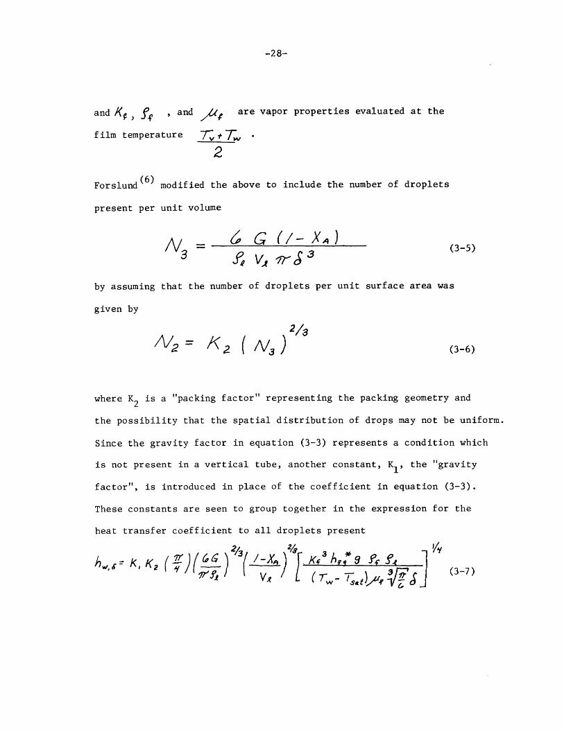
and /( , , and are vapor properties evaluated at the

film temperature ~, T2

Forslund(6) modified the above to include the number of droplets

present per unit volume

6 G (/- X4)N3- (3-5)

by assuming that the number of droplets per unit surface area was

given by

/V2 "2 N 3 (3-6)

where K2 is a "packing factor" representing the packing geometry and

the possibility that the spatial distribution of drops may not be uniform.

Since the gravity factor in equation (3-3) represents a condition which

is not present in a vertical tube, another constant, Ki, the "gravity

factor", is introduced in place of the coefficient in equation (3-3).

These constants are seen to group together in the expression for the

heat transfer coefficient to all droplets present

2/3 2/ 4K2 A 7/- -? -r T 3(3-7)

-29-

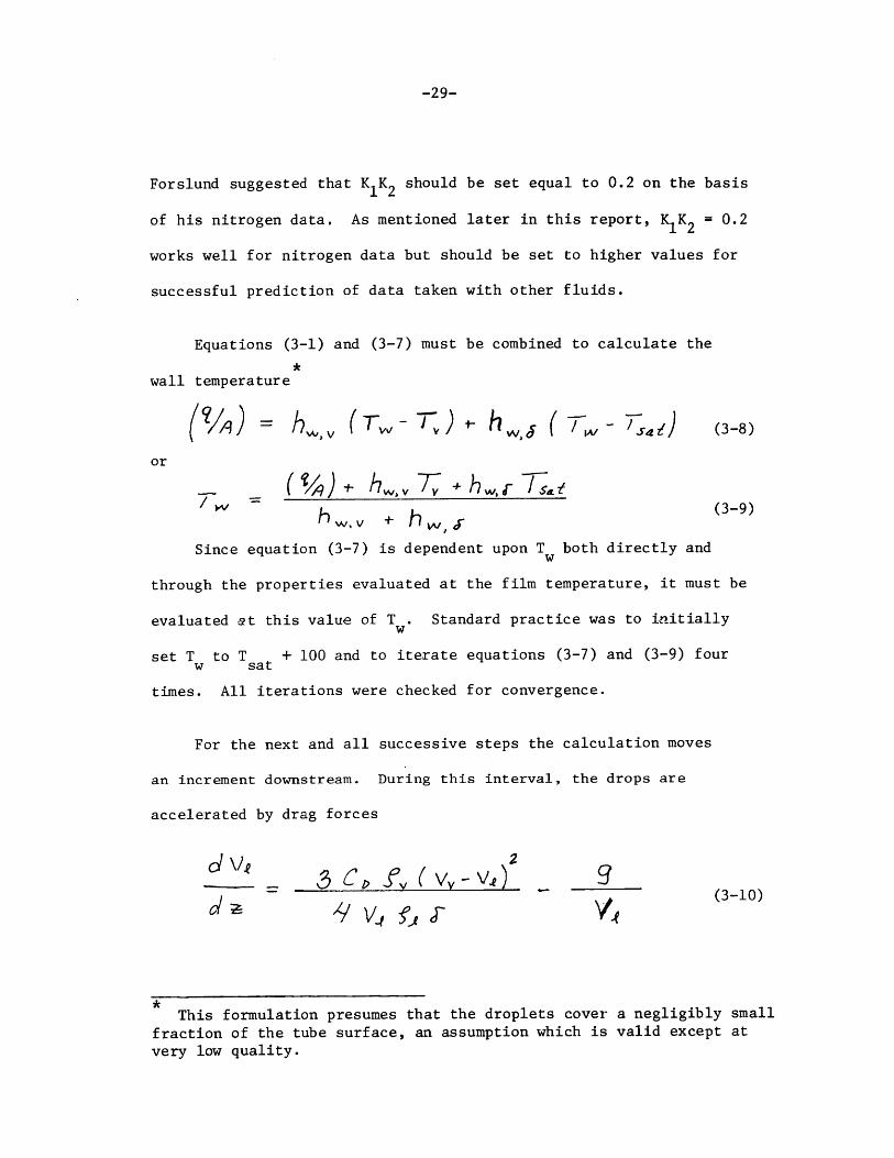
Forslund suggested that KIK2 should be set equal to 0.2 on the basis

of his nitrogen data. As mentioned later in this report, KlK 2 = 0.2

works well for nitrogen data but should be set to higher values for

successful prediction of data taken with other fluids.

Equations (3-1) and (3-7) must be combined to calculate the

*wall temperature

(% )4 = h (r.-T') hW6 (7r- T ) (3-8)

or

(%)+ h±T" + . TI- S(3-9)

Since equation (3-7) is dependent upon T both directly and

through the properties evaluated at the film temperature, it must be

evaluated at this value of T w. Standard practice was to initially

set T to T + 100 and to iterate equations (3-7) and (3-9) fourw sat

times. All iterations were checked for convergence.

For the next and all successive steps the calculation moves

an increment downstream. During this interval, the drops are

accelerated by drag forces

d w 3 ,f (v , __

(3-10)

*This formulation presumes that the droplets cover a negligibly small

fraction of the tube surface, an assumption which is valid except at

very low quality.

-30-

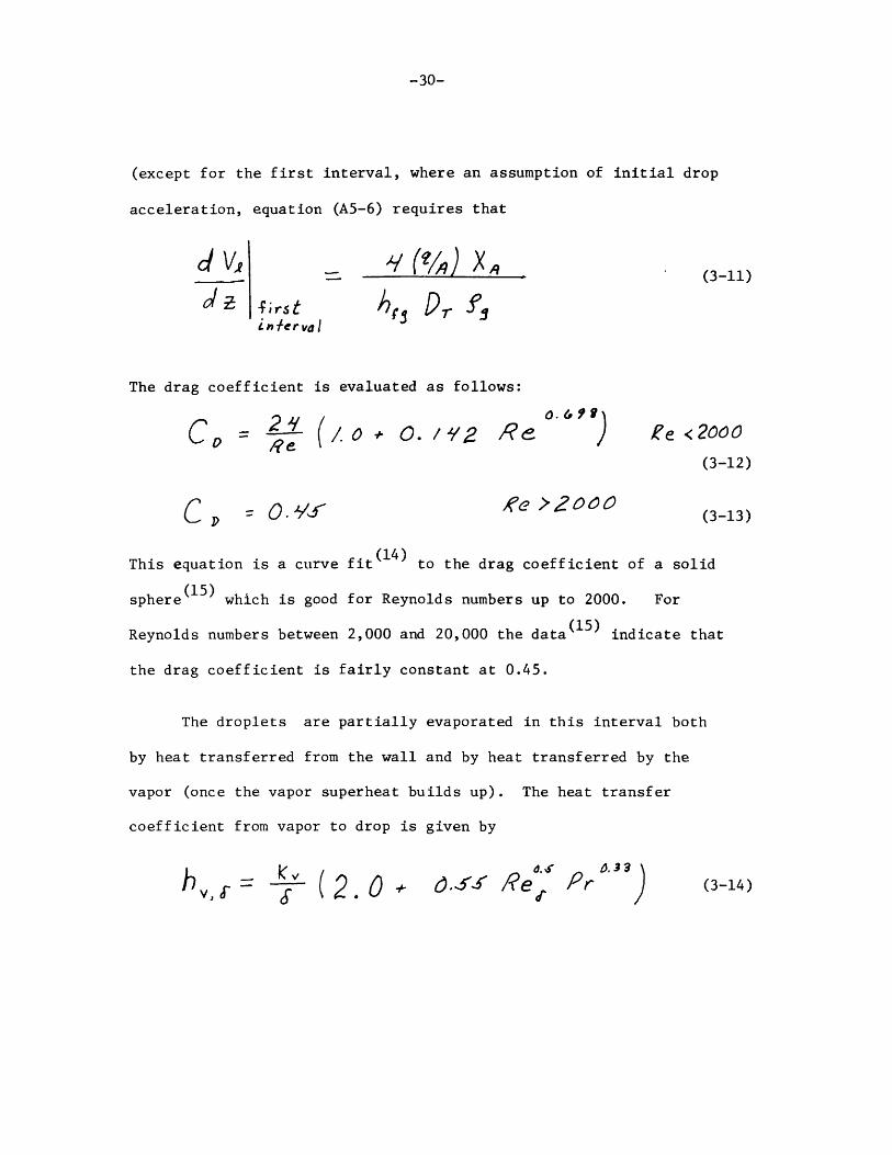
(except for the first interval, where an assumption of initial drop

acceleration, equation (A5-6) requires that

(3-11)

d rst 7 r',in er va I

The drag coefficient is evaluated as follows:

C - 2 1 (/ o +o./y2 Re

C P

0 . C e p .9 1 ) Re <2000(3-12)

)f'e >2000(3-13)

This equation is a curve fit( 14 ) to the drag coefficient of a solid

sphere( 1 5 ) which is good for Reynolds numbers up to 2000. For

Reynolds numbers between 2,000 and 20,000 the data(15) indicate that

the drag coefficient is fairly constant at 0.45.

The droplets are partially evaporated in this interval both

by heat transferred from the wall and by heat transferred by the

vapor (once the vapor superheat builds up). The heat transfer

coefficient from vapor to drop is given by

d.,3S9J5' 1/?e orfP (3-14)J. - K'-v -i-(2-0

-31-

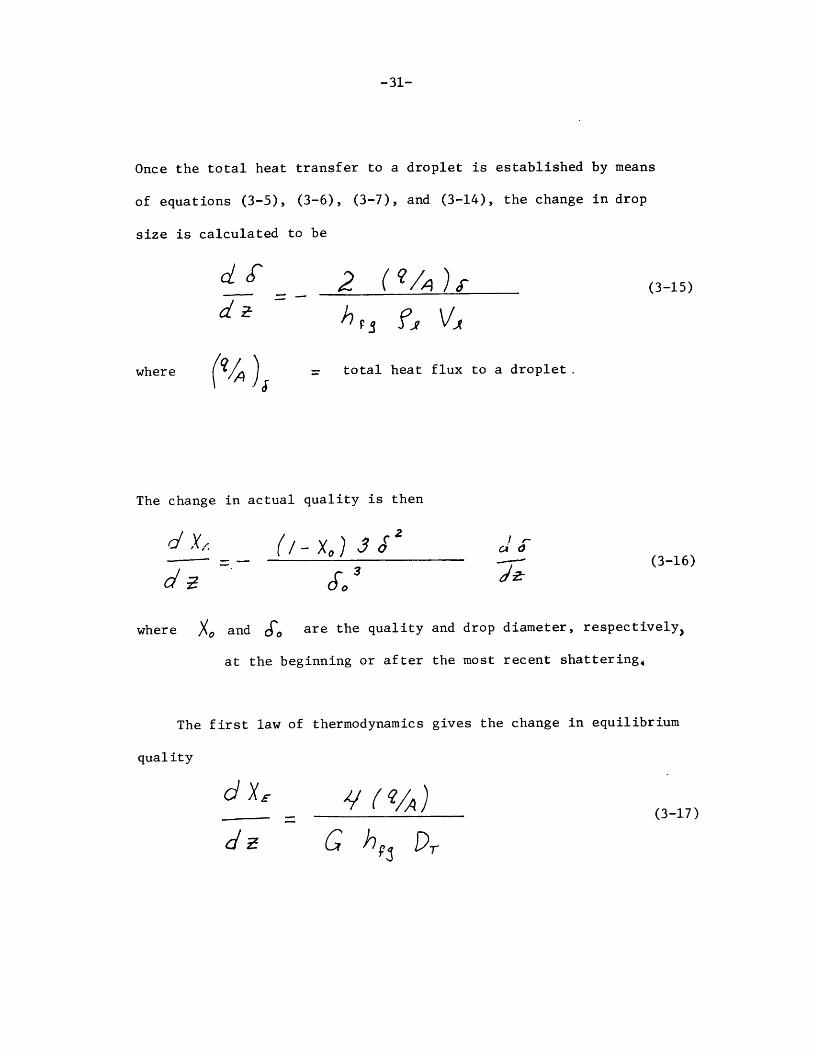
Once the total heat transfer to a droplet is established by means

of equations (3-5), (3-6), (3-7), and (3-14), the change in drop

size is calculated to be

2(de he VX

where

3-15)

total heat flux to a droplet.

The change in actual quality is then

d-X- (i..x) 3c2I,-.

CAd

(3-16)

where XO and & are the quality and drop diameter, respectively,

at the beginning or after the most recent shattering,

The first law of thermodynamics gives the change in equilibrium

quality

dx 4'/ ( q1A)(3-17)

I~ P)'

-32-

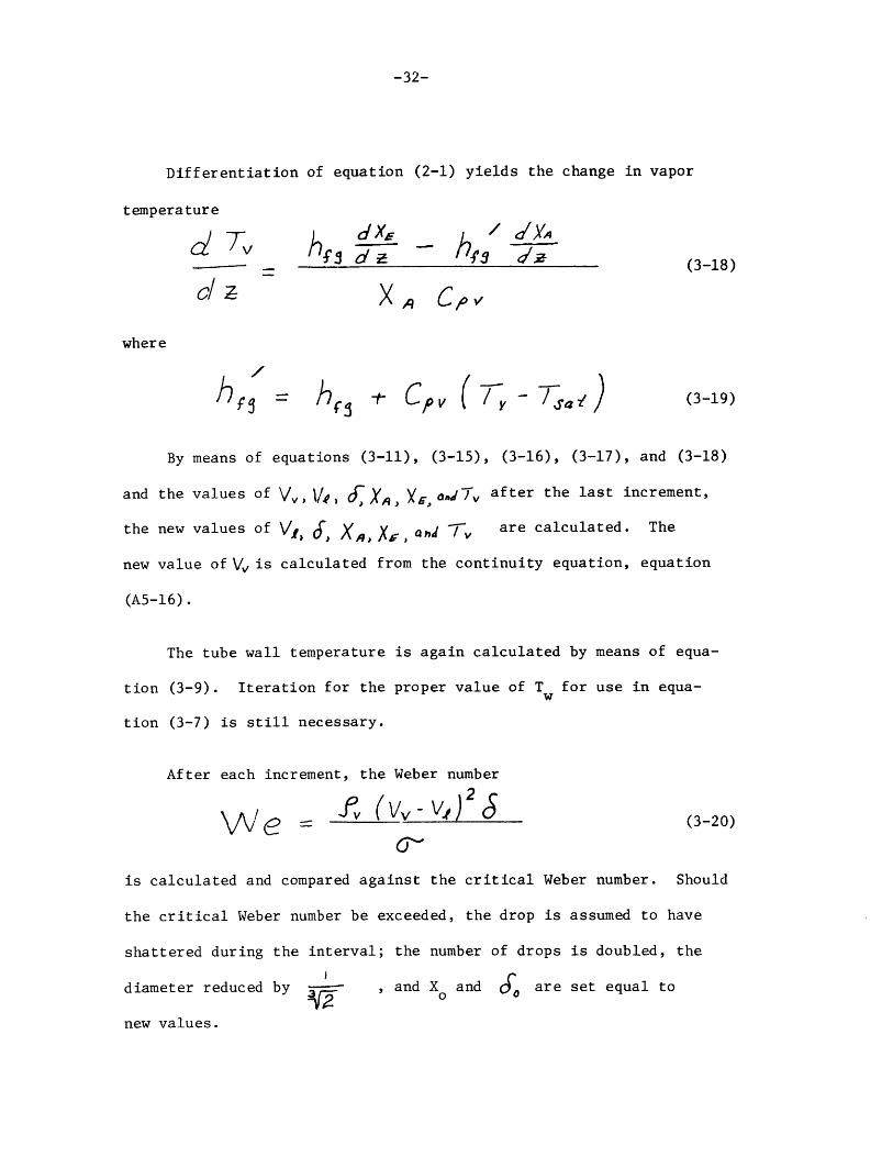
Differentiation of equation (2-1) yields the change in vapor

temperature

---- f - (3-18)/ ZX C-pv

where

h,, ~C) = hY ( , (T -T 3-19)

By means of equations (3-11), (3-15), (3-16), (3-17), and (3-18)

and the values of V,, 1/ P SXA, ) ., after the last increment,

the new values of V 6, X,, )(, and Tv are calculated. The

new value of V is calculated from the continuity equation, equation

(A5-16).

The tube wall temperature is again calculated by means of equa-

tion (3-9). Iteration for the proper value of Tw for use in equa-

tion (3-7) is still necessary.

After each increment, the Weber number

W eV (w- vt 2 S(3-20)G''

is calculated and compared against the critical Weber number. Should

the critical Weber number be exceeded, the drop is assumed to have

shattered during the interval; the number of drops is doubled, the

diameter reduced by , and X and are set equal to

new values.

-33-

The model makes many assumptions. These follow, together with

their justification.

The model assumes that at one point in the tube, thermodynamic

equilibrium exists. This is necessary for setting the initial condi-

tions for calculation. Once the initial vapor velocity, drop velocity,

and drop size are determined (see Appendix 5), vapor superheat can

be accounted for. For a Type II regime, this is taken to be at the

burnout point (more precisely, at the first thermocouple location past

the burnout point), for as noted before, vapor inside a liquid film

cannot be superheated. For a Type I regime, Forslund suggested

initiating the calculation at a quality of about 10%. This point is

not very critical to the calculation, as the non-equilibrium is

small at low quality (see Figure 24). Initiating the calculation at

qualities much below 5% leads to instability in the calculation of

the drop velocity, so one is restricted to larger qualities, around

8% and above. This presents no serious difficulty, as it is difficult

to imagine that dispersed flow exists at such low qualities anyway.

The model assumes that all drops are of the same diameter and

that this diameter is determined by a critical Weber number criterion.

This is obviously a simplification; Cumo, Farello, and Ferrari (16 )

show that the drops follow a normal distribution with a definite

maximum diameter determined by the critical Weber number. However,

it is the larger drops that contain most of the mass and, due to

-34-

their higher slip velocity, do most of the evaporating. The critical

Weber number has been chosen as 7.5, based on data taken by Isshiki(1 7)

Varying this critical Weber number in the calculation produces little

effect, and that only at low qualities.

When a droplet shatters, it is assumed to shatter into two drops,

each containing half the mass (and of the diameter) of the

original droplet. According to pictures of drop shattering taken by

Lane (18), the number of resulting drops is closer to 8 or 10. This

is accompanied by a more substantial change in diameter. However,

by keeping the number down to two, we account, to some degree, for

neglecting the distribution of drop sizes; the drop that doesn't

change its diameter drastically becomes, in effect, the drop that was

not quite big enough to shatter. Isshiki (17) reasons that if the

Weber number of the droplet far exceeds the critical Weber number

(as in the case of a shock wave), the number of droplets resulting

from shattering is large; but if the critical Weber number is exceeded

by only a small fraction, as is the case in dispersed flow, the

number of resultant droplets should only be two. However, Lane's

pictures include drops shattered into many (at least 12) droplets

under free fall conditions.

The coefficient of drag on a liquid drop is assumed to be that

of a solid sphere, as represented by equations (3-12) and (3-13).

This is a departure from Forslund, who used an average of the above

-35-

and of that reported by Ingebo for liquid drops. However,

Buzzard & Nedderman(20) make a convincing case that while the drag

coefficient for liquid drops is a function of such things as liquid

viscosity and surface tension, it does not differ from that of a solid

sphere nearly as much as Ingebo would suggest.

The model assumes that the heat flux is uniform along the test

section. Except for the effects of axial conduction within three

inches or so of the burnout point (see Appendix 6) and within four

inches or so of either end, this is a good assumption for an Inconel

test section. It may not be such a good assumption with the test

sections of other experimenters, generally made of stainless steel;

Forslund allowed for this in his analysis by including in his

original data reduction a correction for the change in electrical

resistivity with temperature. Inasmuch as the other experimenters,

whose data is compared with the model later in this chapter,report

a uniform heat flux, it may be assumed that they did not make this

correction.

The model neglects the pressure gradient along the test section

and the concomitant change in saturation temperature and fluid

properties. The pressure drop is generally quite small and the effects

of the property changes are second order. This is not the case, how-

ever, for the changes of vapor properties with vapor temperature.

The program allows for a linear change with temperature of the

vapor's thermal conductivity, viscosity, and specific heat capacity;

-36-

changes in density are calculated by means of the perfect gas relation.

Over the range of temperature that the vapor reaches, the changes are

small enough so that no large error is introduced by restricting the

change to a linear representation.

The model also assumes that the heat transferred directly from

wall to drop can be calculated from a correlation of data of droplets

film boiling on a flat plate by Baumeister et al.(13) with an empiri-

cally determined constant accounting for the facts that:

(1) not all droplets are in contact with the surface, and

(2) gravity has considerably less effect in a vertical tube

than it has on a horizontal plate.

This constant, herein called K1K2, was found by Forslund to fit his

data reasonably well when set at 0.2.

3.2. Calculations Performed

3.2.1. Prediction of Two Regimes:

One change must be made in Forslund's procedure to predict

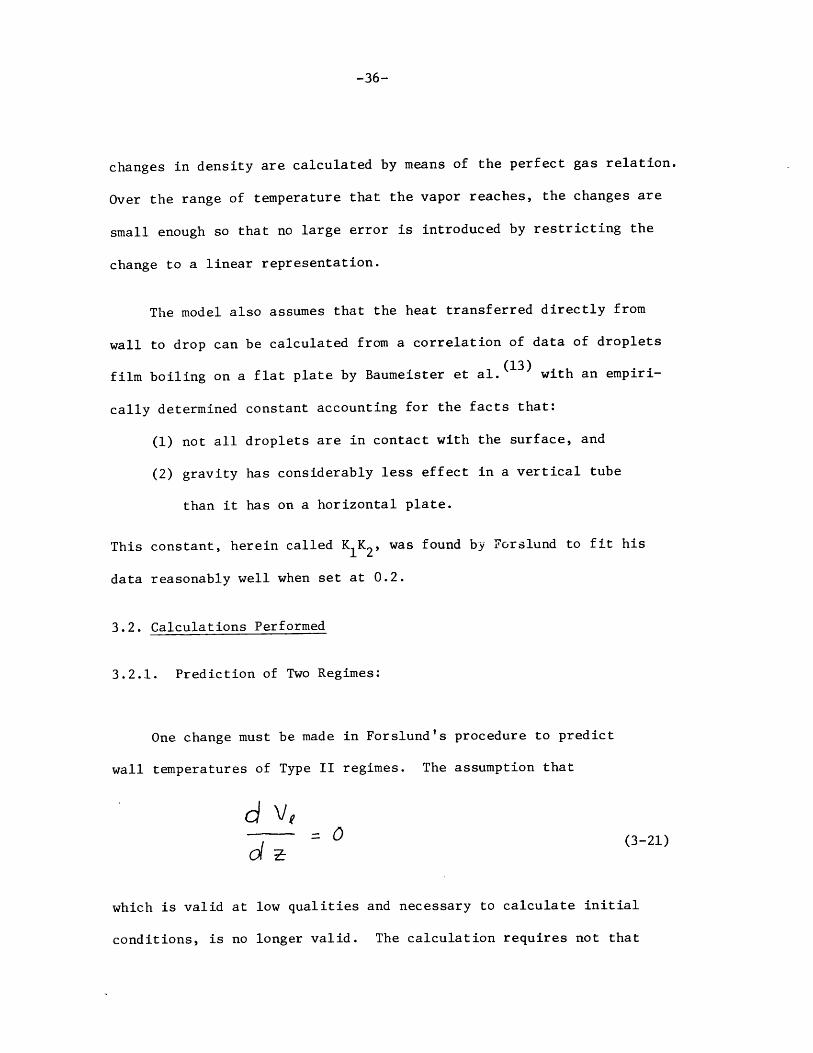
wall temperatures of Type II regimes. The assumption that

d0 (3-21)

which is valid at low qualities and necessary to calculate initial

conditions, is no longer valid. The calculation requires not that

-37-

this derivative equal zero but that it be known. The method outlined

in Appendix 5 is to calculate - and to set

(3-22)

This assumption satisfieG both extremes of XA = 0 and X = 1. Any

positive power of XA would satisfy these extremes, though, and the

choice of one as the exponent is somewhat arbitrary.

The program predicts , for a pair of runs with equal heat and

mass flux and at a given equilibrium quality, that Type I run (#195)

will have a higher wall temperature than the Type II run (#28). Figures

22 and 23 show this; they also show that the data shows the same trend.

Figures 24 and 25 show that this is because the Type I run has greater

non-equilibrium than the Type II run, which in turn is because the

Type II run was in thermodynamic equilibrium upstream of the burnout

point.

Figures 22 and 23 show also that any change in KIK 2 has much more

effect at low quality than at high quality. This, of course, is to

be expected because at high quality there is less liquid. The cal-

culation is made here with more than one value of KIK2 partly to

demonstrate this point and partly to show that 0.2 is a reasonable

choice for K1K2 in the case of nitrogen data. Figures 26 and 27

show the same effect for high mass flux and low heat flux conditions.

-38-

The significance of the existence of two regimes and of the

choice between them afforded by startup procedure is that the

Type II regime has lower wall temperatures than the Type I regime,

given equal heat and mass fluxes. Upstream of the burnout point,

this is due to liquid film on the wall; downstream, lower wall

temperatures are due to lesser thermodynamic non-equilibrium. This

fact is of interest to designers of systems which are temperature-

limited. The lower non-equilibrium of Type II runs also yields a

higher actual quality at the exit; this feature is of interest to

designers of boilers that are meant to connect directly to turbines;

liquid droplets have an adverse effect on the life of turbine blades.

3.2.2. Fluids Other than Nitrogen:

The program was set up to handle any fluid for which both data

and properties were available, as long as the temperatures stayed

below those at which radiation becomes important (Appendix 7 cal-

culates that the temperature above which radiation cannot be

neglected is in the neighborhood of 1400*F). Attempts were made

to predict film boiling data for methane, propane, and water.

3.2.2.1. Methane

Figure 28 shows that KK2 = 0.2 is not acceptable for the meth-

ane data,(23) but that K1K2 = 2.0 may be. Figure 29 shows the results

of using K1K2 = 2.0 for three other methane runs. Twelve inches or

-39-

so after the calculation is begun, the agreement is quite good for

these randomly selected runs.

No good reason immediately presents itself to explain why K K2

should be ten times the value that works for nitrogen. This test

section, like ours, was oriented vertically. The test section dimen-

sions are not greatly different. Their test section was 0.35" I.D.

and 3 feet long, whereas ours was 0.4" I.D. and 8 feet long. Forslund,

who used more than one tube diameter and length, reported that neither

had much effect.

3.2.2.2 Propane

Propane runs tended to group themselves into two categories:

those which, after a foot or so, tended to agree with K K 2= 2.0,

and those which tended to agree with K K 2= 1'0.

Examples of the former, shown in Figures 30 and 31, are charac-

terized by relatively high mass flux and by a relatively low degree

of non-equilibrium (see Figure 32). That the two should go together

is not surprising in view of Figure 5, which shows that the degree

of non-equilibrium decreases as the mass flux increases.

Examples of the latter, shown in Figures 33 and 34, are charac-

terized by lower mass flux and more non-equilibrium, as shown by

Figure 35. Again, consider Figure 5, which shows that the degree

of non-equilibrium increases as the mass flux decreases.

-40-

3.2.2.3. Water

Agreement between theory and the data of Mueller(2 1 ) for 1000

psi water is poor. However, agreement between the data of one run

and the next seems poor, too.

Except for run #5 (Figure 37), the agreement between theory

and experiment is generally within 150*R, or about 25% of T - Tw sat

for this data of water at 1000 psi (Figures 36 through 39). The

program indicates very little rise in actual quality as the calcu-

lation progresses up the test section. This is due primarily to

the high heat of vaporization of water, as Appendix 8 will attest.

It is strange that while run #5 has less than 10% more heat

flux than run #6, it has roughly 45% higher difference between the

measured wall and saturation temperatures, although mass flux and

quality are the same. This would suggest that one of these runs

(probably #5) is in error.

Figures 40 through 43 show that agreement between the theory

and the data of Bennett et. al.(22) is much better. The effects

of end conduction, discussed earlier, are evident in these figures,

as the experimental wall temperatures drop at the right-hand end of

the graphs. In the theoretical calculations, K1 K2 was arbitrarily

set equal to one. Since the theory gave consistently higher wall

temperatures than were observed experimentally, more so at lower

-41-

qualities, the choice of a higher value of K1K2 is indicated.

The proper value of K1K2 seems to be a function of the fluid.

One value of K1K2 can satisfactorily account for most data for a

particular fluid, whereas a different value will satisfactorily

account for another fluid.

The data for both methane and propane were provided by M. R.

Glickstein (23). Properties for nitrogen were obtained from

references 24 and 25; properties of methane were obtained primarily

from reference 24; properties of propane were obtained primarily

from reference 26; properties of water were obtained primarily

from reference 27. These properties are listed in Appendix 8.

3.3. Twisted Tape

Modification of the program so that it can predict data taken

with the twisted tape installed requires changing the wall-to-vapor

heat transfer coefficient to allow for the swirling vapor by re-

placing equation (3-1) with equation (2-13), the equation best

describing the single phase twisted tape data of section 2.3.2.4.

The wall-to-drop heat transfer coefficient, equation (3-7),

requires two changes. First the gravity factor g must be replaced

by the centrifugal acceleration

/ (3-23)

-42-

Second, the empirical constant K K2 must be changed to reflect the

new physical situation. Since the model is no longer dealing with

the hypothetical fraction of gravity referred to in section 3.1 and

represented by K1, but with the entire centrifugal acceleration, K1

should now be set equal to 1.1. The model for the physical situation

existing with the twisted tape no longer assumes that droplets exist

everywhere within the tube, but that the droplets are all near the

tube wall, at a distance from the wall where centrifugal force is

balanced by the Leidenfrost force. As the Leidenfrost force is

very localized, having an inverse fourth power dependence on dis-

tance between the drop and the wall, (28) this distance is quite

small and all droplets can be considered to be essentially at the

tube wall for purposes of calculating the centrifugal acceleration.

The packing factor referred to in section 3.1 and referred to by

K2, should now be greater than for the tube without the twisted

tape. This is not to imply that the wall is covered with drops;

at any but the lowest qualities, the void fraction is too high

to permit this. At the low qualities near the inlet, an excep-

tion is made, as explained below. The product K K2, which essen-

tially replaced the coefficient of equation (3-3), should again

be determined by the data and equation (3-7) is replaced by

x_ 2/7)(I-A) [ (3-24)

-43-

Figures 44 through 47 show results of calculations using the

twisted tape model for both regimes and for both degrees of tape

twist. Here calculations were made for K K2 equal to 0, 1, and 2.

K K2 = 1.5 appears to be the best choice, but the data seems to be

bounded roughly by K1 K2 = 0.5 and K 1K2 = 2.5. This deviation from

the predicted temperatures seems to indicate that two changes to

the model are necessary.

First of all, at the beginning of the test section the swirl

flow of the vapor is not established immediately but the centrifuging

effect takes a finite length to become developed. This means that

near the test section entrance the drops are not all near the wall,

and the packing factor must reflect this. K K2 cannot be as high

as it would be downstream. This idza is strengthened by the obser-

vation that in Figure 45, with y = 4.1, the experimental and theo-

retical temperature profiles cross in one half the length that is

required for those of Figure 46, with y = 8.5, to cross; the tape

with y = 4.1 has roughly half the pitch of the tape with y = 8.5,

so it takes one half the length to rotate the flow the required

number of turns to put the drops on the wall.

Second, it appears that the empirically determined value of

KIK2 is roughly 1.5.

-44-

CONCLUSIONS AND RECOMMENDATIONS

4.1 Conclusions

To be concluded are the following:

1) There are two distinct regimes of forced convection dispersed

flow film boiling. Which occurs depends on the manner in which

the operating point is reached; their dissimilarity in heat

transfer coefficient is due to different degrees of non-

equilibrium; and transition from one regime to the other is

greatly affected by conduction at the test section entrance.

2) Installation of a twisted tape increases the heat transfer

coefficient by a factor of 2 or 3 and can, for high mass fluxes,

cause re-establishment of a liquid film on the wall near the

test section exit.

3) There is definite evidence that a liquid streamer forms on the

twisted tape:

a) Droplets are observed at exit qualities greater than one,

indicating more non-equilibrium than should be expected

with the tape.

b) The quality at burnout is decreased by the presence of the

twisted tape.

-45-

4) The modified calculation procedure of Laverty and Forslund,

based on thermodynamic non-equilibrium, is capable of pre-

dicting the data of other experimenters within 10% in regions

unaffected by axial conduction using fluids other than

nitrogen; however, an unexplained change in the empirical

constant governing the direct wall-to-droplet heat transfer

is necessary.

4.2 Recommendations

1) Visual evidence of the streamer should be gathered, perhaps

most easily by extending the twisted tape into the visual

test section and photographing the streamer.

2) Experiments with film boiling of water at high temperatures

should be made, and the analysis thereof should include the

effects of radiation from wall to drop.

3) For purposes of augmentation, the plain twisted tape should

be replaced by a tape with an occasional hole in the center

or by twisted internal fins; this would eliminate the streamer.

-46-

REFERENCES

1. Kruger, R. A., "Film Boiling on the Inside of Horizontal Tubesin Forced Convection", Ph.D. Thisis, MIT Dept. of Mech. Eng.,June, 1961.

2. Dougall, R. S., and W. M. Rohsenow, "Film Boiling on the Insideof Vertical Tubes with Upward Flow of the Fluid at LowQualities", MIT, Dept. of Mech. Eng., EPL Report No. 9079-26,Sept., 1963.

3. Laverty, W. F., and W. M. Rohsenow, "Film Boiling of SaturatedLiquid Flowing Upward Through a Heated Tube: High VaporQuality Range", MIT, Dept. of Mech. Eng., EPL Report No.9857-32, Sept., 1964.

4. Laverty, W. F., and W. M. Rohsenow, "Film Boiling of SaturatedNitrogen Flowing in a Vertical Tube", ASME Paper 65-WA/HT-26,1965.

5. Forslund, R. P., and W. M. Rohsenow, "Thermal Non-Equilibriumin Dispersed Flow Film Boiling in a Vertical Tube", MIT,Dept. of Mech. Eng., EPL Report No. 75312-44, November,1966.

6. Forslund, R. P., and W. M. Rohsenow, "Dispersed Flow Film Boiling",ASME Journal of Heat Transfer, 90 (1968), 4, pp. 399-407.

7. Fuller, W. D., "Swirl Flow in Dispersed Flow Film Boiling", MIT,Dept. of Mech. Eng., S. M. Thesis, September, 1968.

8. Lopina, R. F., and A. E. Bergles, "Heat Transfer and PressureDrop in Tape Generated Swirl Flow", MIT, Dept. of Mech. Eng.,EPL Report No. 70281-47, June, 1967.

9. Thorsen, R., and F. Landis, "Friction and Heat Transfer Charac-teristics in Turbulent Swirl Flow Subjected to Large Trans-verse Temperature Gradients", ASME Journal of Heat Transfer,90 (1968), 4, pp. 87-97.

-47-

10. Petukhov, B. S., V. V. Kirillov, and V. N. Mardanik, "HeatTransfer Experimental Research for Turbulent Gas Flow inPipes at High Temperature Difference Between Wall and BulkFluid Temperature", Proceedings of the Third InternationalHeat Transfer Conference, Vol. 1, August, 1966.

11. Taylor, M. F., "Experimental Local Heat Transfer Data for

Precooled Hydrogen and Helium at Surface Temperatures up

to 5300 Deg. R", NASA TND-2595, January 1965.

12. McAdams, W. H., Heat Transmission, 3rd Ed., McGraw-Hill,

New York, 1954.

13. Baumeister, K. J., T. D. Hamill, and G. J. Schoessow, "A

Generalized Correlation of Vaporization Times of Drops inFilm Boiling on a Flat Plate", US-A.I.Ch.E.-No. 120,

Third International Heat Transfer Conference and Exhibit,

August 7-12, 1966.

14. Kent, J. C., General Motors Research Laboratory, personal

communication, 1966.

15. Eisner, F., 3rd Int. Cong. App. Mech., Stockholm, 1930.

16. Cumo, M., G. E. Farello, and G. Ferrari, "Notes on Droplet Heat

Transfer", Comitato Nazionale Energia Nucleare, Rome, Italy.

17. Isshiki, N., "Theoretical and Experimental Study on Atomization

of Liquid Drop in High Speed Gas Stream", Report No. 35,

Transportation Technical Research Institute, Tokyo, Japan.

18. Lane, W. R., "Shatter of Drops in Streams of Air", Ind. and Eng.

Chem., 43 (1951), pp. 1312-1317.

19. Ingebo, R. D., "Drag Coefficients for Droplets and Solid Spheres

in Clouds Accelerating in Airstreams", NACA TN 3762, September,

1956.

20. Buzzard, J. L., and R. M. Nedderman, "The Drag Coefficients of

Liquid Droplets Accelerating Through Air", Chem. Eng. Sci.,

Vol. 22 (1967), pp. 1577-1586.

-48-

21. Mueller, R. E., "Film Boiling Heat Transfer Measurements in aTubular Test Section", GEAP-5423 (1967).

22. Bennett, A. W., G. F. Hewitt, H. A. Kearsey, and R. F. F. Keeys,"Heat Transfer to Steam-Water Mixtures Flowing in UniformlyHeated Tubes in which the Critical Heat Flux Has Been Exceeded",AERE-R5373, 1967.

23. Glickstein, M. R., Pratt & Whitney Aircraft Co., personal com-munication, 1967.

24. Thermophysical Properties Research Center Data Book, Vol. 2.

25. Strobridge, T. R., "The Thermodynamic Properties of Nitrogenfrom 114 to 540 *R between 1.0 and 3000 psia, Supplement A(British Units)'' NBS Tech. Note 129A, February, 1963.

26. A Compendium of the Properties of Materials at Low Temperatures,WADD TR 60-56, July, 1960.

27. Keenan, J. H. and F. G. Keyes, Thermodynamic Properties of Steam,Wiley, New York, 1936.

28. Hynek, S. J., "The Effect of Duct Curvature on Dispersed Flow",MIT 2.57 Term Paper, May, 1967.

29. Rohsenow, W. M., and H. Y. Choi, Heat, Mass, and Momentum Trans-fer, Prentice-Hall, 1963.

30. Chemical Rubber Co. Standard Mathematical Tables, 12th edition.

31. Sparrow, E. M., and R. D. Cess, Radiation Heat Transfer, Brooks/Cole, 1966.

32. Moeck, E. O., G. A. Wikhammer, I. P. L. MacDonald, and J. G.Collier, "Two Methods of Improving the Dryout Heat Flux forHigh Pressure Steam/Water Flow", AECL-2109, December 1964.

-49-

APPENDIX 1

MEASUREMENT OF THE POWER FACTOR

The power dissipated by an electric heater is given by

P= V A Cos < (Al-i)

where is the phase angle between the voltage and current. This

phase angle comes about because a hollow tube is not a purely resis-

tive load but has some inductance.

To measure the power factor, the voltmeter was connected to the

X axis of an oscilliscope and the ammeter to the Y axis, thus genera-

ting a Lissajous figure which indicated the phase lag. The results

are shown in Figure 48 . The average value of the power factor was

measured to be 0.94. The fact that there is no apparent dependence

of power factor on power level may be interpreted to mean that the

power factor is due only to constant factors, such as the tube induc-

tance, and not to factors that vary with power level, such as satura-

tion of transformers.

Note: An independent power factor evaluation was made after this report

was completed. It was found that the actual power factor was 0.99;

hence, there is a small error in some of the data reported for nitrogen.

-50-

APPENDIX 2

DERIVATION OF TEMPERATURE DIFFERENCE ACROSS TUBE WALL

Let( 9A)be the heat flux on the inside wall if no heat were lost

through the outisde wall. Let F be the fraction of the heat generated

in the tube that is lost through the outer wall. Let W/1 be the heat

generated per unit volume of tube. Let, , K, Il, and r. be the length,

conductivity, inside and outside radii , respectively, of the tube.

Since neither the resistivity, conductivity, nor density of Inconel 600

change rapidly with temperature and since temperature differences

calculated by this method never exceed 5 *F, constant properties can

be assumed.

A/ is calculated from A

2 Ji(r2 r )

Heat loss through the outside wall is taken to be the fraction Fof the heat generated, yielding the boundary condition

-- F Wiri~ 2 (A2-2O~U d r io UT2

or

dF I\ r-

-51-

Given a uniform \A/ and K , we can make use of the standard (29)

solution to the conduction equation in cylindrical coordinates.

(A2-4)

This must also apply at r = r

Tz-vv r 2+ (A2-5)

Equation (A2-5) can be differentiated to make use of the boundary

condition implied by equation (A2-3)

C T W C,---- - - - f' + -- - c- C

dr 21 r. X

Solving equation (A2-6) for C1 , we get

(A2-6)

(A2-7)C = - ( ) r + W r,

Equation (A2-7) is now inserted into equation (A2-5) and the result

is solved for C

=T, + r2& (r2r_ 2 (A2-3)~1

- 2 + cr+ ,

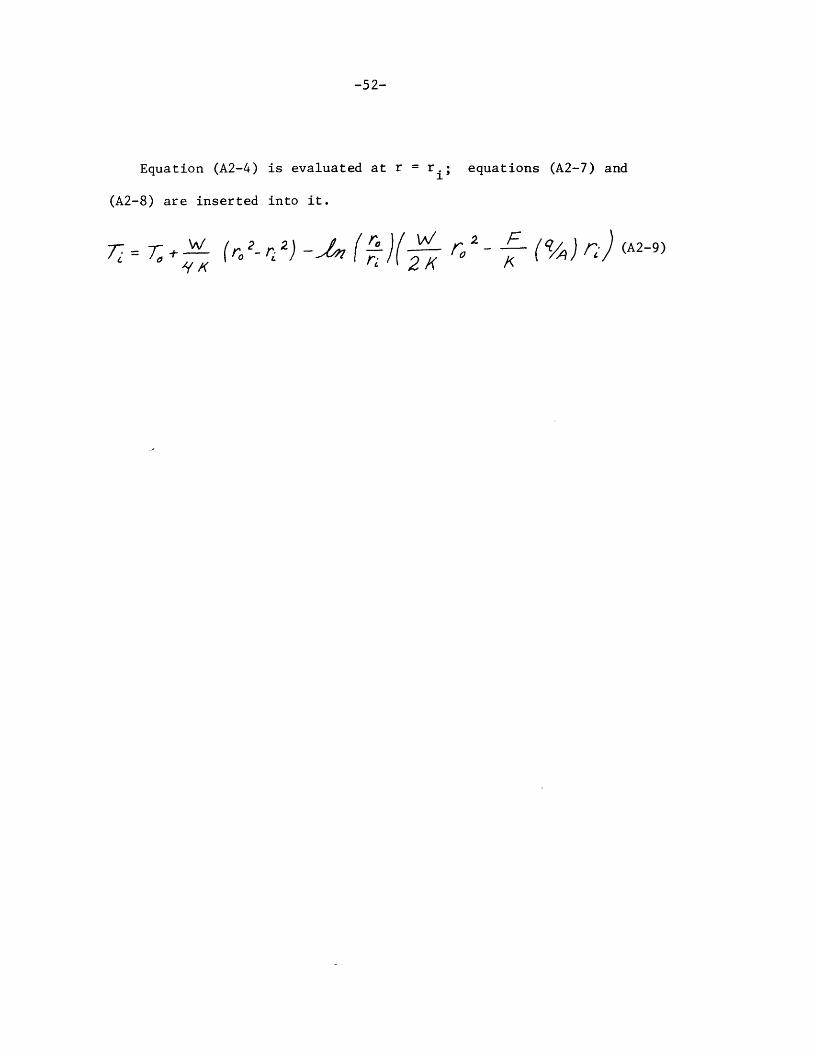
-52-

Equation (A2-4) is evaluated at r = ri; equations (A2-7) and

(A2-8) are inserted into it.

=7 + (r 2_ 2( I / -'; (A2-9)

-53-

APPENDIX 3

MEASUREMENT OF THE MINIMUM HEAT FLUX

The minimum heat flux that could support a Type I regime (film

boiling beginning at the test section entrance) was measured under

both sets of conditions shown in Figure 49; that is, for the cases

of thermal conduction into and out of the inlet flange via the

power line. The minimum heat flux was determined by establishing a

Type I regime with a mass flux of 40,000 lb m/ft -hr, and by decreasing

the power incrementally until the vapor film at the entrance collapsed,

as indicated by a sharp decrease in the temperature monitored by the

flange thermocouple. After each power change, the system was allowed

to reach steady state.

Figure 49A shows the case of conduction into the test section.

For this case, the heat transmitted to the fluid is the sum of the

heat generated in the tube and that conducted in through the power

connection. The minimum heat flux was observed to be 2,200 Btu/ft -hr;

the flange thermocouple read 220*R at this point. Data were taken at

other mass fluxes, and the results were very nearly the same (see

Reference 7).

Figure 49B shows the case of conduction away from the test sec-

tion. This was brought about by the guard cooler mentioned in

section 2.1.2.4. For this case, the heat transmitted to the fluid

is the difference between the heat generated in the tube and that

conducted away by the power connection. The minimum heat flux was

observed to be 18,700 Btu/ft -hr; the flange thermocouple read

452*R at this point.

-5 4-

From the difference in the measured heat fluxes it is apparent

that the heat conducted into or away from the test section inlet is

considerable.

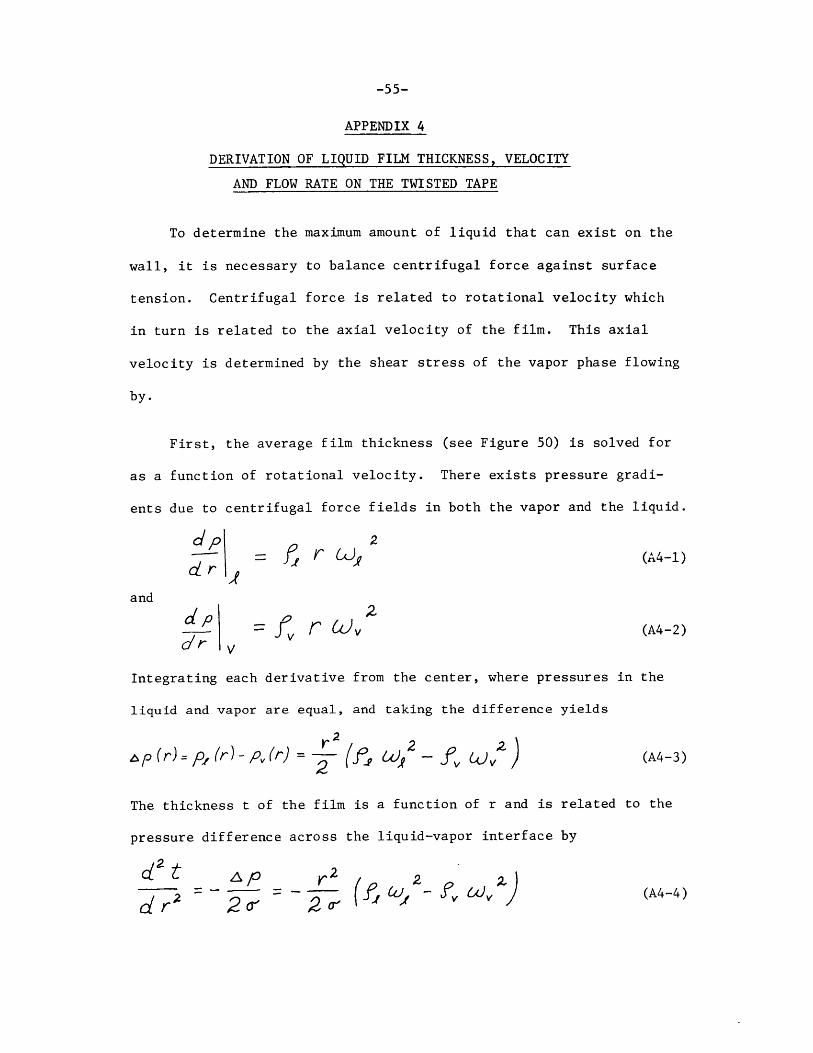
-55-

APPENDIX 4

DERIVATION OF LIQUID FILM THICKNESS, VELOCITY

AND FLOW RATE ON THE TWISTED TAPE

To determine the maximum amount of liquid that can exist on the

wall, it is necessary to balance centrifugal force against surface

tension. Centrifugal force is related to rotational velocity which

in turn is related to the axial velocity of the film. This axial

velocity is determined by the shear stress of the vapor phase flowing

by.

First, the average film thickness (see Figure 50) is solved for

as a function of rotational velocity. There exists pressure gradi-

ents due to centrifugal force fields in both the vapor and the liquid.

dip 2'-~rW (A4-1)

d rand

fvr (tv (A4-2)C/ rV

Integrating each derivative from the center, where pressures in the

liquid and vapor are equal, and taking the difference yields

op ()=0v (r) ' vU (A4-3)

The thickness t of the film is a function of r and is related to the

pressure difference across the liquid-vapor interface by

C 2 t 2 2c~~r'~6 2cr fl (FV W v; (A-4)

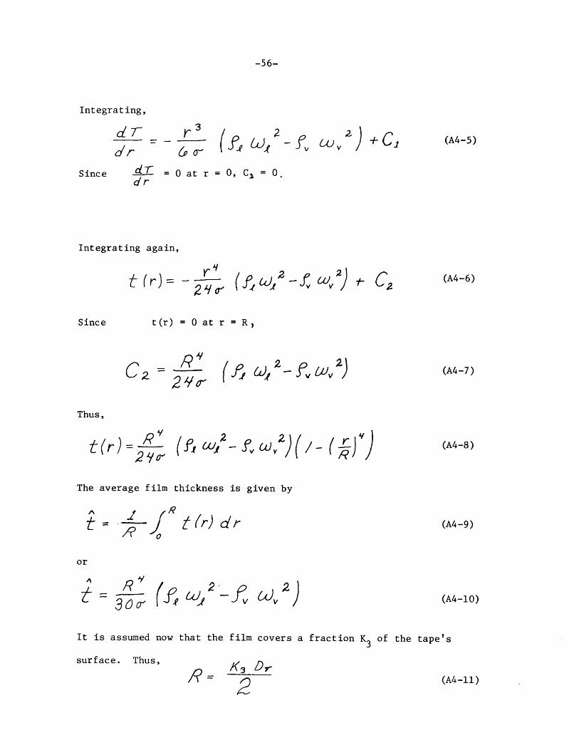
-56-

Integrating,

' 7 - -- 3

0/r &a-~

Since

( 'eW bi

-d 7 = 0 at r = 0, C, = 0.dr

Integrating again,

Since t(r) = 0 at r = R,

(A4-7)

Thus,

2 1r

.2p - (fecUj"fi'

The average film thickness is given by

^ = -p

t (r) dr

/

36c~ (,G~ (Lb2. Wv 2)

It is assumed now that the film covers a fraction K3 of the tape's

surface. Thus,

(A4-ll)

2j + Oc (A4-5)

( W -- 2 EAf v 2) C2(A4-6)

(A-8)

(A4-9)

(A4-10)

Y, A

C2 r ( - , <4e 2- FV WV2)

K3 D7-

2

WY;Z(/ (R)

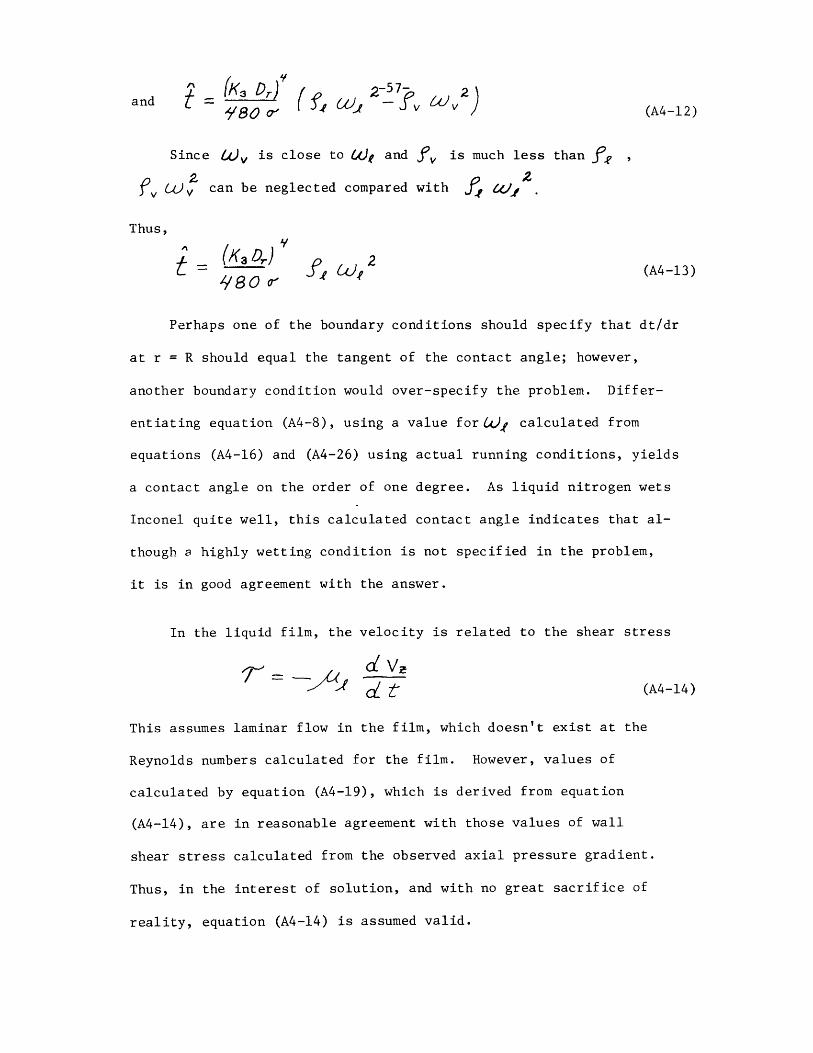
and ( (A4-12)

Since w, is close to We and f, is much less than

v W2 can be neglected compared with f a4/

Thus,

_(K' 3Dr)~-(8) 2 (A4-13)

Perhaps one of the boundary conditions should specify that dt/dr

at r = R should equal the tangent of the contact angle; however,

another boundary condition would over-specify the problem. Differ-

entiating equation (A4-8), using a value for (i)1 calculated from

equations (A4-16) and (A4-26) using actual running conditions, yields

a contact angle on the order of one degree. As liquid nitrogen wets

Inconel quite well, this calculated contact angle indicates that al-

though a highly wetting condition is not specified in the problem,

it is in good agreement with the answer.

In the liquid film, the velocity is related to the shear stress

2 d L'(A-14)

This assumes laminar flow in the film, which doesn't exist at the

Reynolds numbers calculated for the film. However, values of

calculated by equation (A4-19), which is derived from equation

(A4-14), are in reasonable agreement with those values of wall

shear stress calculated from the observed axial pressure gradient.

Thus, in the interest of solution, and with no great sacrifice of

reality, equation (A4-14) is assumed valid.

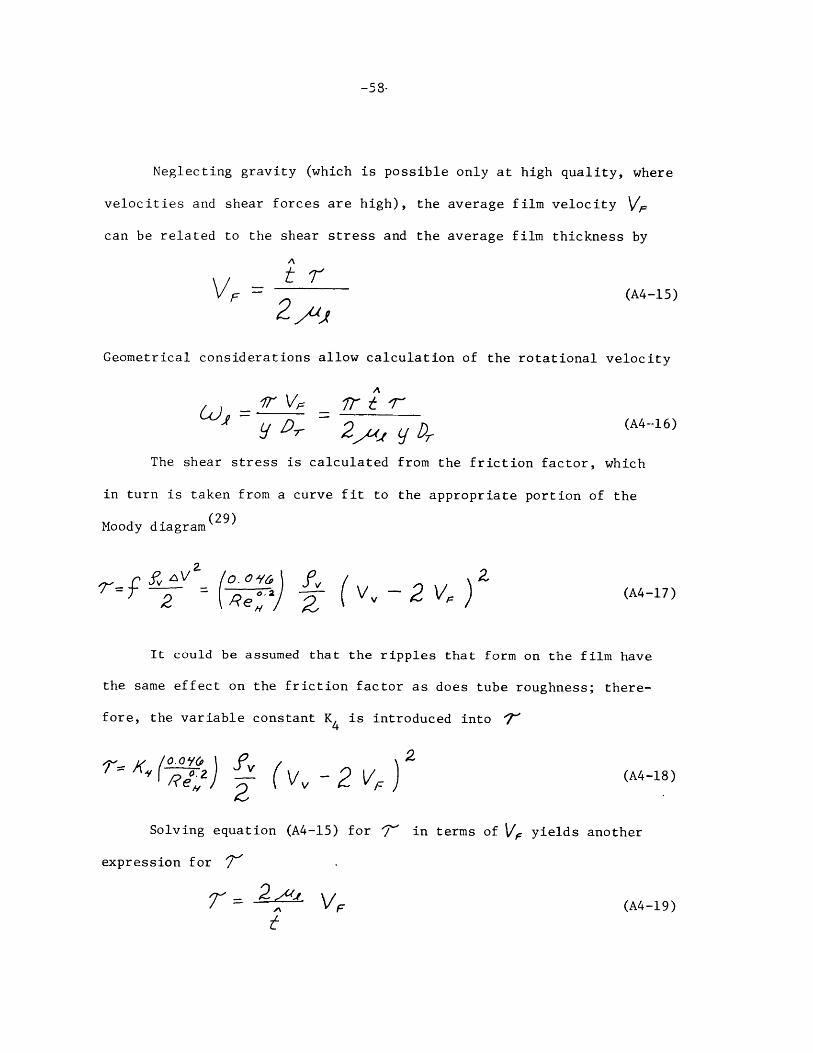
-5-'S

Neglecting gravity (which is possible only at high quality, where

velocities and shear forces are high), the average film velocity V,can be related to the shear stress and the average film thickness by

A

tVF (A4-15)

Geometrical considerations allow calculation of the rotational velocity

A

f) n (A4-16)

The shear stress is calculated from the friction factor, which

in turn is taken from a curve fit to the appropriate portion of the

Moody diagram(2 9)

2 (v- 2 V (A-17)2 Re212 v

It could be assumed that the ripples that form on the film have

the same effect on the friction factor as does tube roughness; there-

fore, the variable constant K is introduced into 7'

2 / -(A4-18)

Solving equation (A4-15) for 7 ' in terms of V, yields another

expression for 7'

2 V(A4-19)

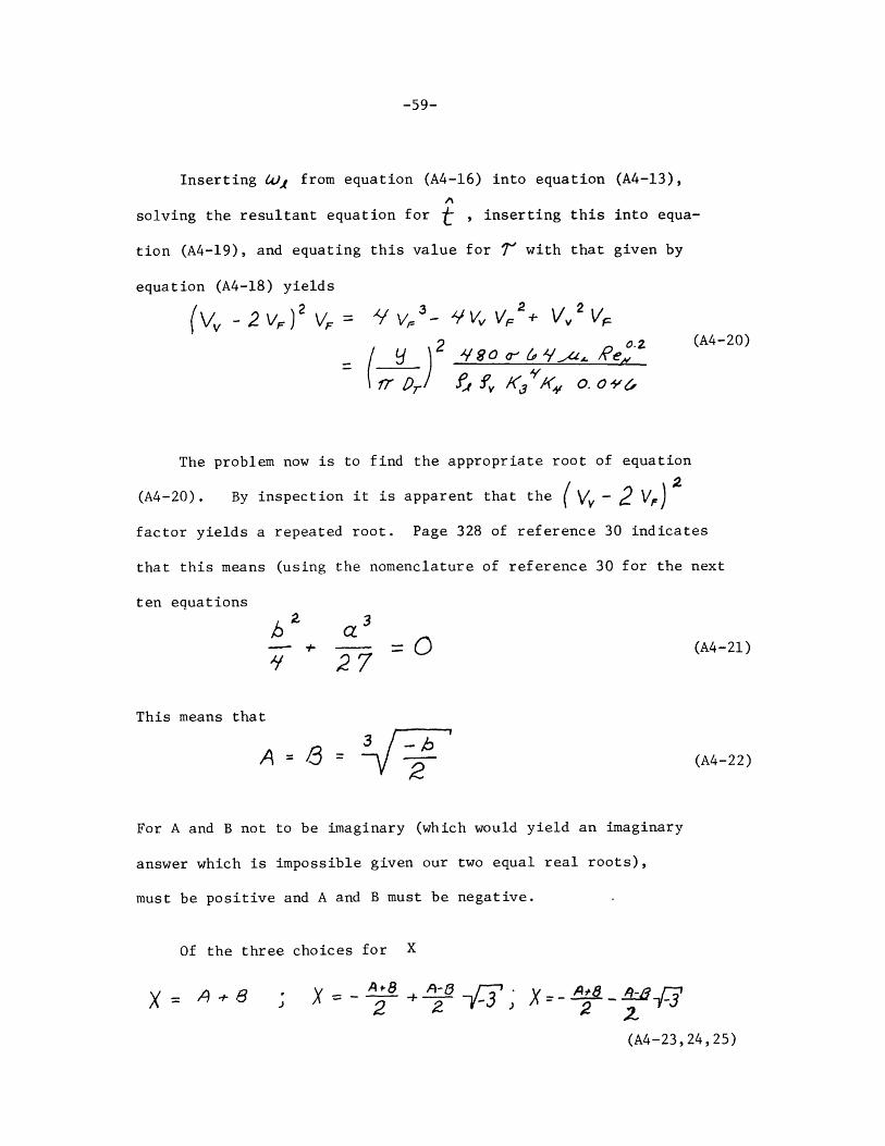
-59-

Inserting UW, from equation (A4-16) into equation (A4-13),

solving the resultant equation for t , inserting this into equa-

tion (A4-19), and equating this value for ' with that given by

equation (A4-18) yields

(v/ - 2 v,) VF 2' V Vv + V" 2 VF)2 v.2 (A4-20)2 1/ 80 <r' ( A/l : Ze(A 20

Wr Dr fv A'AvK 0. -,l 6

The problem now is to find the appropriate root of equation

(A4-20). By inspection it is apparent that the ( \v -2 2

factor yields a repeated root. Page 328 of reference 30 indicates

that this means (using the nomenclature of reference 30 for the next

ten equations

Q a--- 7= 0(A4-21)

This means that

-3 (A4-22)

For A and B not to be imaginary (which would yield an imaginary

answer which is impossible given our two equal real roots),

must be positive and A and B must be negative.

Of the three choices for X

A(48 -23 24, 2'0q X C--42 27~3(A-23 , 24, 25)

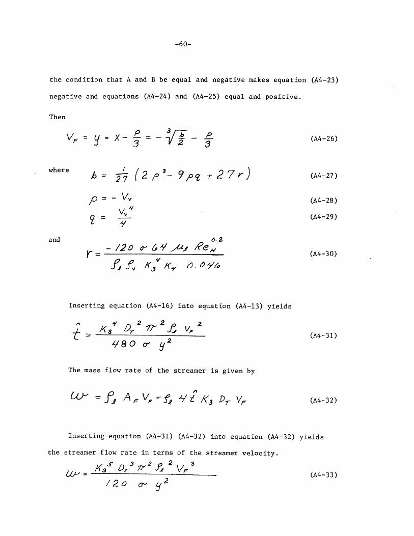
-60-

the condition that A and B be equal and negative makes equation (A4-23)

negative and equations (A4-24) and (A4-25) equal and positive.

Then

F 2 (A4-26)

where ( 3 - ?p 2 7 (A-27)

(A4-28)

- (A4-29)

and c. 2

- /2 O - 6;Y 7A4 /2es2 (A4-30)

Vf 3 K,,

Inserting equation (A4-16) into equation (A4-13) yields

1K3 Dr -f(A4-31)

480 Yog2

The mass flow rate of the streamer is given by

Wj A p --fAFY 4Z K3 7~ VF (A4-32)

Inserting equation (A4-31) (A4-32) into equation (A4-32) yields

the streamer flow rate in terms of the streamer velocity.

# )3 2 2 32 ' (A4-33)

/20 Y

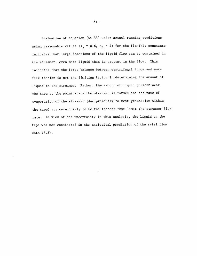
-61-

Evaluation of equation (A4-33) under actual running conditions

using reasonable values (K3 = 0.6, K = 4) for the flexible constants

indicates that large fractions of the liquid flow can be contained in

the streamer, even more liquid than is present in the flow. This

indicates that the force balance between centrifugal force and sur-

face tension is not the limiting factor in determining the amount of

liquid in the streamer. Rather, the amount of liquid present near

the tape at the point where the streamer is formed and the rate of

evaporation of the streamer (due primarily to heat generation within

the tape) are more likely to be the factors that limit the streamer flow

rate. In view of the uncertainty in this analysis, the liquid on the

tape was not considered in the analytical prediction of the swirl flow

data (3.3).

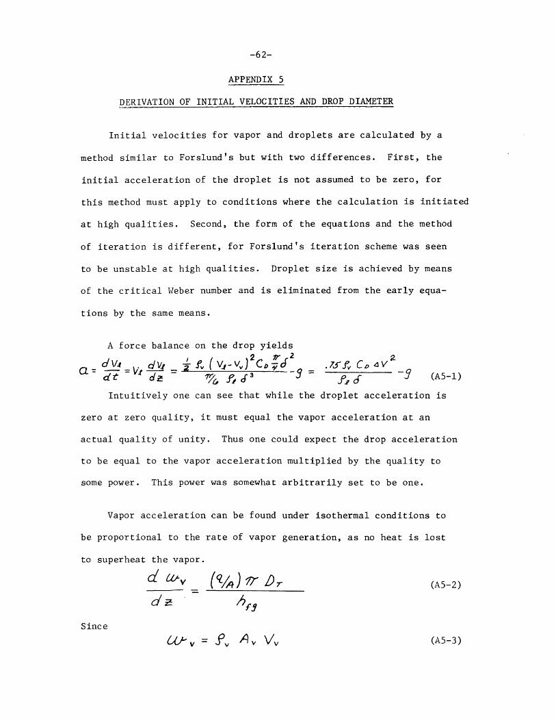
-62-

APPENDIX 5

DERIVATION OF INITIAL VELOCITIES AND DROP DIAMETER

Initial velocities for vapor and droplets are calculated by a

method similar to Forslund's but with two differences. First, the

initial acceleration of the droplet is not assumed to be zero, for

this method must apply to conditions where the calculation is initiated

at high qualities. Second, the form of the equations and the method

of iteration is different, for Forslund's iteration scheme was seen

to be unstable at high qualities. Droplet size is achieved by means

of the critical Weber number and is eliminated from the early equa-

tions by the same means.

A force balance on the drop yields

d ~ dg ~ '1vr 3) - ~_ -_- (A5-1)

Intuitively one can see that while the droplet acceleration is

zero at zero quality, it must equal the vapor acceleration at an

actual quality of unity. Thus one could expect the drop acceleration

to be equal to the vapor acceleration multiplied by the quality to

some power. This power was somewhat arbitrarily set to be one.

Vapor acceleration can be found under isothermal conditions to

be proportional to the rate of vapor generation, as no heat is lost

to superheat the vapor.

d aV (V )Yr r (A5-2)

Since

&t-v = ' v A v \v (A5-3)

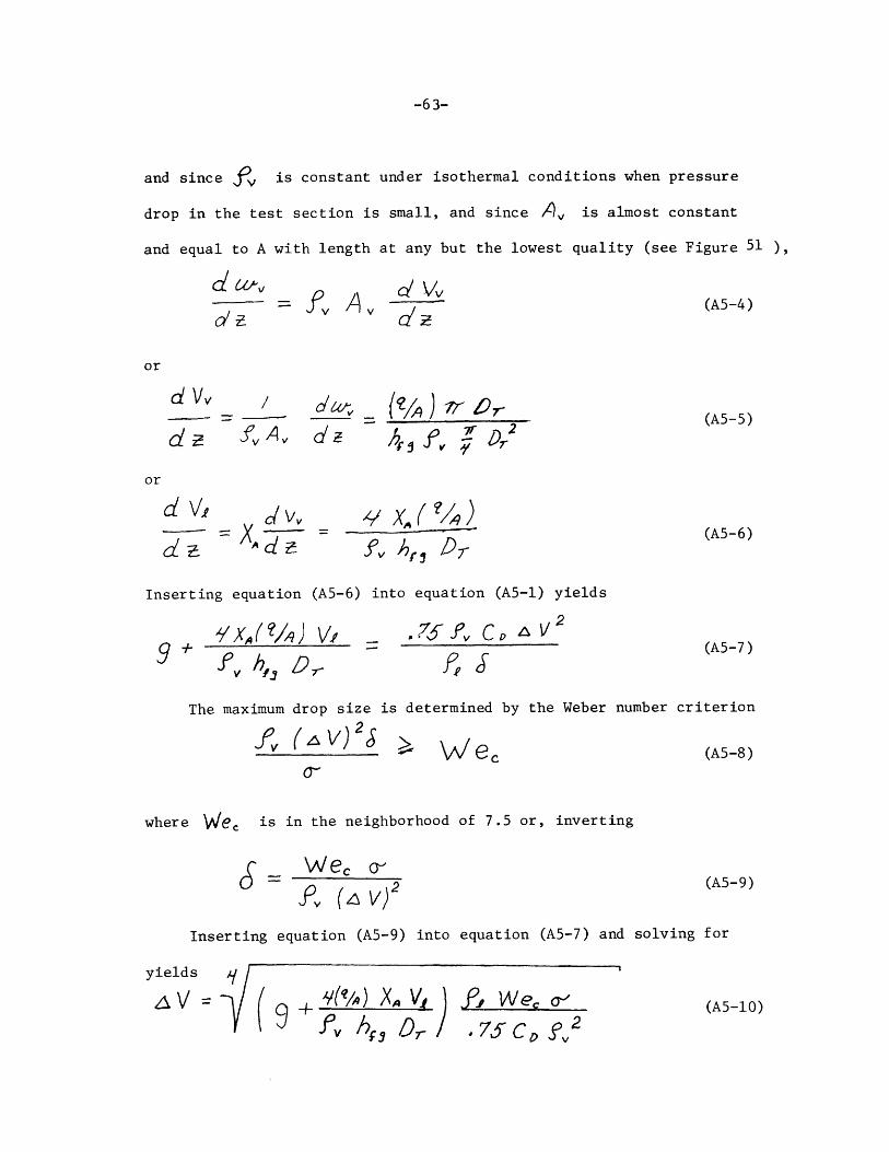
-63-

and since f, is constant under isothermal conditions when pressure

drop in the test section is small, and since Av is almost constant

and equal to A with length at any but the lowest quality (see Figure 51 ),

-- -V (A5-4)

or

- _ _ 7 -- (A5-5)

d h;3Av da ~ )

or

? A ) (A5-6)

Inserting equation (A5-6) into equation (A5-1) yields

p9 C(A5-7)

v h13407

The maximum drop size is determined by the Weber number criterion

f V W ec (A5-8)0-~

where Wec is in the neighborhood of 7.5 or, inverting

WeOc a~'We - 2 (A5-9)Jv (z V)2

Inserting equation (A5-9) into equation (A5-7) and solving for

yields l

~' v h75CrD, .75 CD f

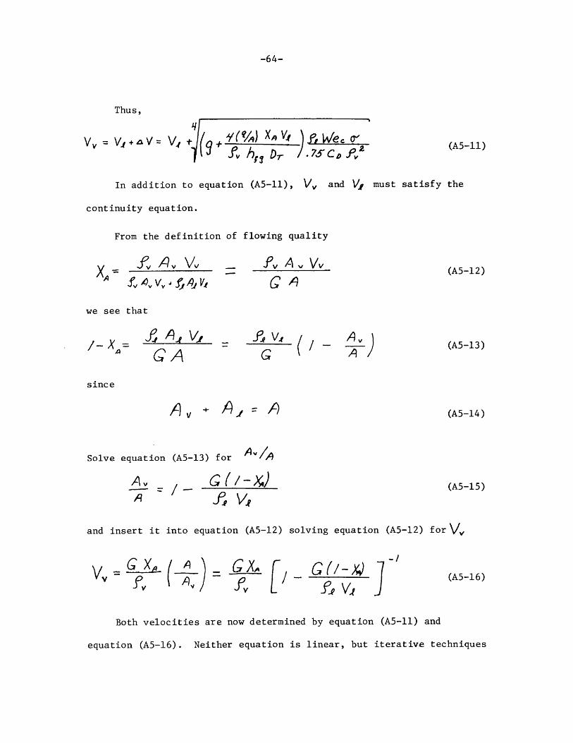
-64-

Thus,

VV= V. ,aV = V, 7(9Y( MA) X'9 V4 f~Wc+ We r- /ll

In addition to equation (A5-ll), V. and

continuity equation.

From the definition of flowing quality

X =f, V4 fAj V,

(A5-11)

V, must satisfy the

-v A v Vv(A5-12)

we see that

f Aps V;Av,

GA GC

since

V +

Solve equation (A5-13) for

A /- G / / -XA fe V1

AvA)

(A5-13)

(A5-14)

(A5-15)

and insert it into equation (A5-12) solving equation (A5-12) for V

--C(/-x) 7- (A5-16)

Both velocities are now determined by equation (A5-1) and

equation (A5-16). Neither equation is linear, but iterative techniques

A _ X-4V =G ( t

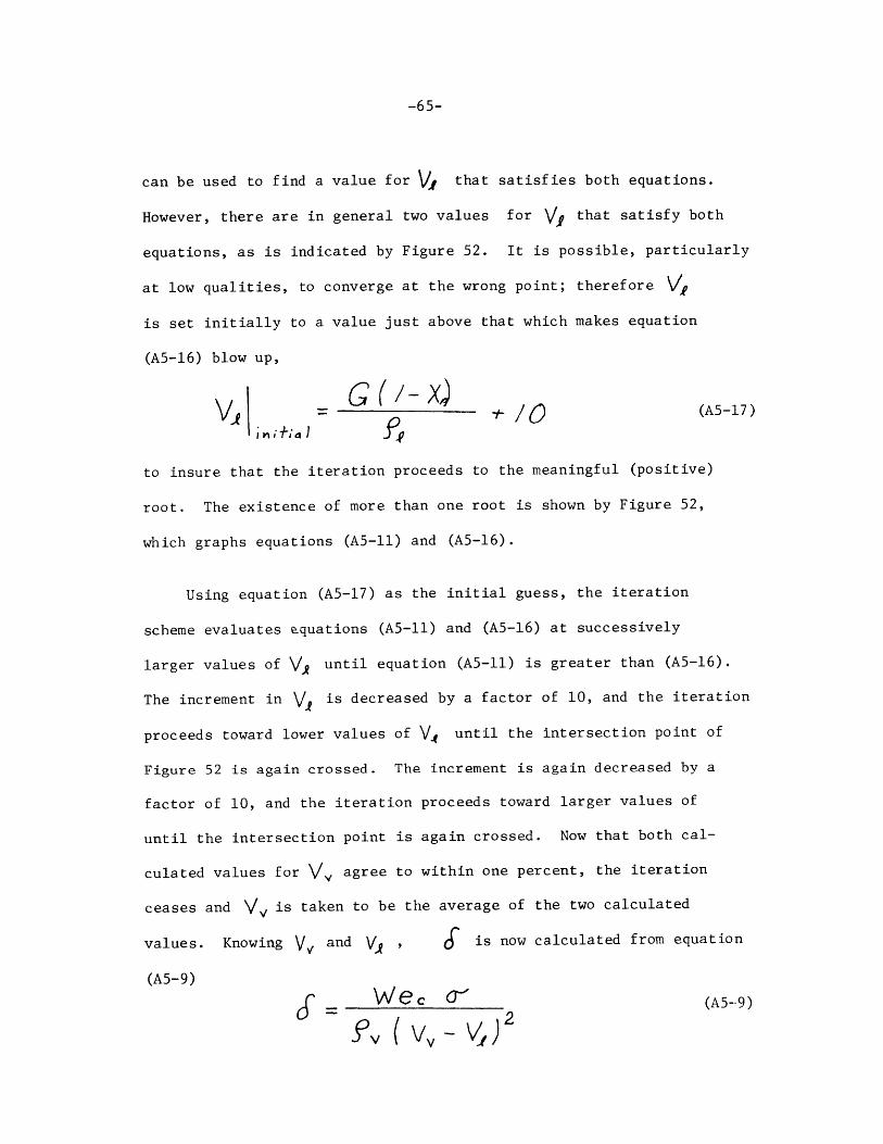
-65-

can be used to find a value for Vj that satisfies both equations.

However, there are in general two values for V, that satisfy both

equations, as is indicated by Figure 52. It is possible, particularly

at low qualities, to converge at the wrong point; therefore Vis set initially to a value just above that which makes equation

(A5-16) blow up,

G({/-x X,,)0V, X) -, / (A5-17)

to insure that the iteration proceeds to the meaningful (positive)

root. The existence of more than one root is shown by Figure 52,

which graphs equations (A5-ll) and (A5-16).

Using equation (A5-17) as the initial guess, the iteration

scheme evaluates e.quations (A5-ll) and (A5-16) at successively

larger values of \/g until equation (A5-ll) is greater than (A5-16).

The increment in V, is decreased by a factor of 10, and the iteration

proceeds toward lower values of V4 until the intersection point of

Figure 52 is again crossed. The increment is again decreased by a

factor of 10, and the iteration proceeds toward larger values of

until the intersection point is again crossed. Now that both cal-

culated values for \/ agree to within one percent, the iteration

ceases and \/ is taken to be the average of the two calculated

values. Knowing \f and V is now calculated from equation

(A5-9)

\/ec o~' (A5-9)

V \ v ,2

-66-

In evaluating equation (A5-1l), the value of Cp is taken to

be 0.45. After the iteration is finished, the Reynolds number of the

drop is calculated. If it is less than 2000, a new value of CD is

calculated from equation (3-12); the iteration is begun anew and

repeated four times to converge on an acceptable value for C 0.

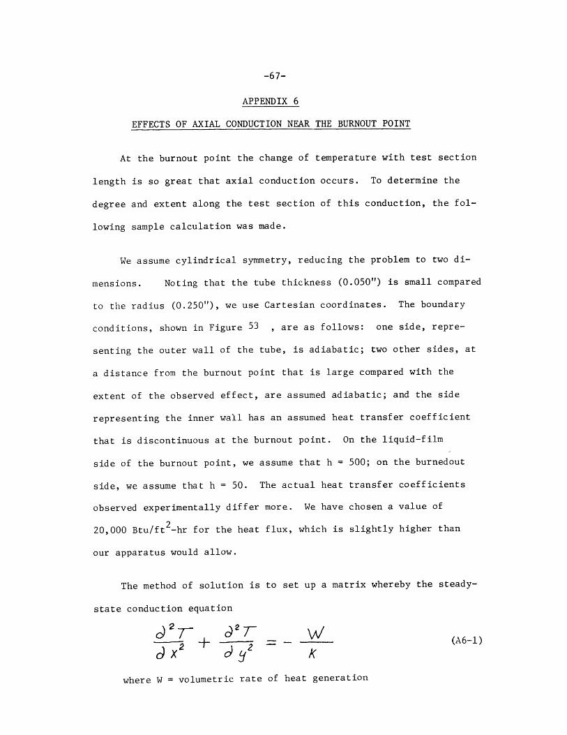
-67-

APPENDIX 6

EFFECTS OF AXIAL CONDUCTION NEAR THE BURNOUT POINT

At the burnout point the change of temperature with test section

length is so great that axial conduction occurs. To determine the

degree and extent along the test section of this conduction, the fol-

lowing sample calculation was made.

We assume cylindrical symmetry, reducing the problem to two di-

mensions. Noting that the tube thickness (0.050") is small compared

to the radius (0.250"), we use Cartesian coordinates. The boundary

conditions, shown in Figure 53 , are as follows: one side, repre-

senting the outer wall of the tube, is adiabatic; two other sides, at

a distance from the burnout point that is large compared with the

extent of the observed effect, are assumed adiabatic; and the side

representing the inner wall has an assumed heat transfer coefficient

that is discontinuous at the burnout point. On the liquid-film

side of the burnout point, we assume that h = 500; on the burnedout

side, we assume that h = 50. The actual heat transfer coefficients

observed experimentally differ more. We have chosen a value of

20,000 Btu/ft -hr for the heat flux, which is slightly higher than

our apparatus would allow.

The method of solution is to set up a matrix whereby the steady-

state conduction equation

- __(A6-1)

dX2 92K

where W = volumetric rate of heat generation

-68-

is satisfied at the 176 nodes shown in Figure 53 . Once we have

the temperatures, we use the two rows of nodes nearest the inner

wall to give us the temperature gradient, thus heat flux, across

the inner wall. Both the inner wall temperature and the heat flux

are shown in Figure 54 .

As can be seen, the effect of axial conduction, the disruption

of uniformity of the heat flux, extends only an inch or so to either

side of the burnout point.

-69-

APPENDIX 7

EFFECT OF RADIATION

It is rather obvious that the effect of radiation is negligible

for film boiling of cryogenic fluids, but is not so readily apparent

that it can be neglected for film boiling of water. The temperatures

reported by Mueller (21) are as high as 1400*F. The following are

sample calculations for radiation from wall to vapor and from wall

to drop.

Radiation from Wall to Vapor;

We shall evaluate the worst possible case, Let the tube wall

temperature be 1400*F, as in Run 5 for Mueller's (21) water data.

It is difficult to use the Hottel Mean Beam Length (29) method, for

the pressure is too high to allow calculation of the correction factor

for converting the emissivity at 1 atm. to that at our 1000 psi pres-

sure by means of the published graph; however, the absorptivity of

the vapor cannot be any greater than one, so we will use this value

for our worst-case calculation. The emissivity of stainless steel

can be as high as 0.97 (when oxidized); however, a long tube can

look like a cavity to the gas, so we can set the wall emissivity

equal to one, especially for our worst case. When the vapor is not

superheated at all, corresponding to the worst case, its temperature

is 1005*R. Thus, the heat flux is given by

( T- T r'n 8 _ _ (A7-1)

r4d;4JO. W, V W- h r

-8 Btuwhere 0' = Stefan-Boltzmann constant = 0.171 x 10 2 4

ft -hr-*R

-70-

This value is pretty small compared to the 292,000 Btu/ft -hr heat

flux leaving the tube wall.

Radiation from Wall to Drop:

Here again we can set the wall emissivity, for the worst case,

equal to one. The absorptivity of a water drop can be calculated

given its temperature and size; the calculation is long, as one must

determine an effective wavelength above which water absorbs essen-

tially all radiation. This wavelength appears to be about 2 microns.

According to Planck's black body energy distribution (31), roughly

90% of the energy emitted by a black surface at 1860*R is above 2

microns in wavelength and is thus absorbed. However, since this is

a rough idea of the absorptivity and since this is a worst-case

calculation, we shall set the absorptivity equal to one.

Equation (1) yields the same value as before. This must be

compared with the heat flux entering the drop, as calculated by the

analytical program. The calculated heat flux to the droplet depends

strongly on K K2 = 0 and 72,400 for K K2 = 2.

This should mean that the addition of radiation to the analytical

program for this run would be roughly equivalent to increasing K 1K2

by 0.5, which in turn would result in decreasing the calculated wall

temperature by 50*R. All this is based on the reported wall tempera-

ture of 1800*R. Were the radiation calculations based on the highest

calculated wall temperature (remember, Run 5 was the least trusted of

-71-

the reported data), with K1K2 = 0, of 1780*R, we would have calcu-

lated a radiation heat flux of 15,700. Were the calculation based

on the highest calculated wall temperature, with K K 2= 2, of 17000R,

the radiation heat flux would be 13,100, or 18% of the heat flux

calculated without radiation.

Radiation should account for a larger portion of the wall-to-drop

heat transfer for drops smaller than the maximum size considered here.

The radiation heat flux is independent of drop size, whereas the con-

vective heat flux decreases with drop size, for the slip velocity

decreases with decreasing drop size.

The conclusion is that radiation can be ignored if the wall

temperatures are low, say below 1300*R, or if any significant measure

of wall to drop heat transfer already exists.

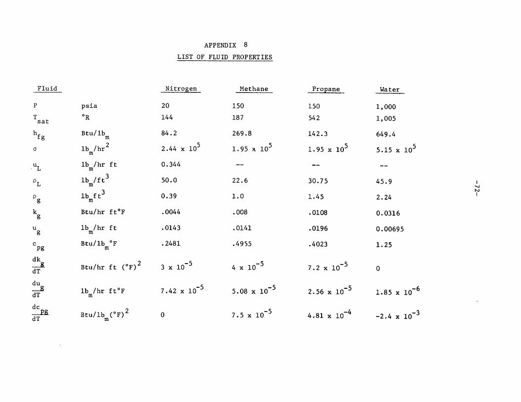
APPENDIX 8

LIST OF FLUID PROPERTIES

Fluid

psia

Tsat

h fg

a

u L

Btu/lb

lb /hr2m

lb /hr f tm

lb /ft3m

lb ft 3

m

Btu/hr ft*F

lb /hr ftm

Btu/lb OFm

Btu/hr ft (OF) 2

lb /hr ft*Fm

Btu/lb m(OF) 2

Nitrogen

20

144

84.2

2.44 x 10 5

0.344

50.0

0.39

.0044

.0143

.2481

3 x 10- 5

7.42 x 10-5

Methane

150

187

269.8

1.95 x 105

22.6

1.0

.008

.0141

.4955

4 x 10-5

5.08 x 10-5

7.5 x 10 -5

Propane

150

542

142.3

1.95 x 10 5

30.75

1.45

.0108

.0196

.4023

7.2 x 10-5

2.56 x 10-5

4.81 x 10~4

Water

1,000

1,005

649.4

5.15 x 105

45.9

2.24

0.0316

0.00695

1.25

1.85 x 10-6

-2.4 x 10-3

dk

dT

du

dT

dc

dT

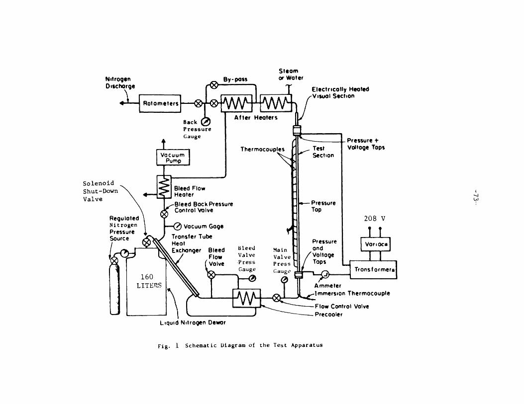
Steamor Water

SolenoidShut-Down Bleed FlowShut-Dow -4 HeaterValve

-nI..,4 Rnek pe~a.ra Pressure

Liquid Nitrogen Dewor

Fig. 1 Schematic Diagram of the Test Apparatus

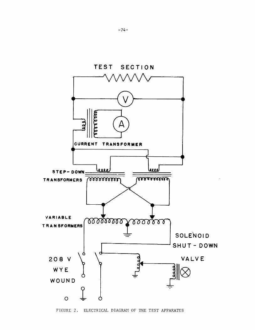
-74-

TEST SECTION

STEP- DOWN

TRANSFORMERS

VARIABLE

T R A N SFORMERS

208 V

WYE

WOUNDW -=E

SOLENOI D

SHUT- DOWN

VALVE

ELECTRICAL DIAGRAM OF THE TEST APPARATUSFIGURE 2.

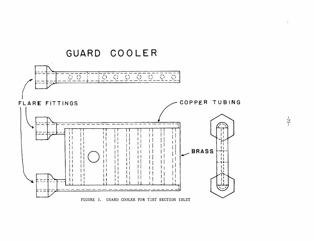
GUARD COOLER

COPPER

B (B RA SZE

TUBING

FIGURE 3. GUARD COOLER FOR TZST SECTION INLET

FLAR

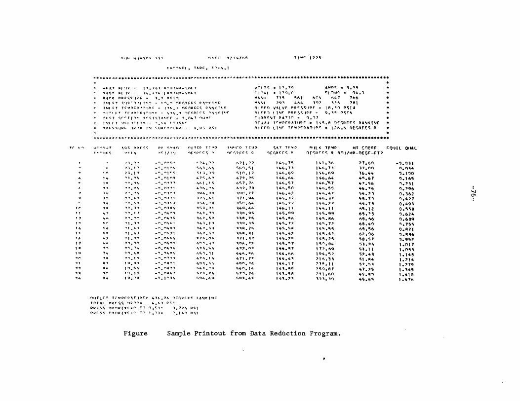
rATr q/144/A TiAC 177F

imenrj , TApe, 77=4.1

***************************** * ********** *** **.********.*************************

4r AT F 'l -IV 11,741 CkT1/4:)-5(lV T

%Age F C, = F1, )1 In4 /1O-r TPt srK nOrs'C laF = 3.7 1 -T1111 -t' ,'I T I = ) 10.' ')rr Fr Dn'v T,?;

TKIlCT TrUDCDAT'IOr = 1 *c.) rcruOC es OANK TfiIrt F T TrAnroT1rc - 41,.1 -)rF Or r II

T&: -,T 4r'TT)% S)rcSTAmrr =1.047 n"Mc

I i r T \e Iqr y Ty : '. cg r/4 T / c c

'1o rc e'llo a): 10 y-q 4 11ptenoi Fu , q.111 o)4;1

Vrl TS = 1.70 AMoC = 3.Aq *rI ,wl = 1 79.' r WR = 94.1 *

MANH 73i FAI 4r.4 447 746

MANI 791 404 307 124 71 *

FI CFO VILVF D 1S4'10r = I A.1 0 A *RI CF) I JNr POFSSoIQF - Q.3F pst4SIrIqorNT PATIn = C).7 *

0rIA-t TrMPrOA IIJ1 = 14.F ')ERFFS RAN'(JINF *

Al rsn IjNC TFMDCoATI'oc , 1?A.4 EGr)EqFFS a*

***~~~~~~~** a****~****a*********a*****a***************.***************************

r , r 4T r PA, nors rP' n"sA nIlTeD Tr-4D IvovrO TCr, AP %AT TCr%0 IrL[( TF14P HT CnEF FT1J1. QI0ALT hor LS ' C' v CN / 1F".DrC-S I qrr,9FCC Q 'FqQCFC 0: 13.E FRrps R ATIJ/4P-0EGF-FT?

'3.6 ,-.1 7

17.1 0

4171.1 31

'1.4*l

'1.*41

' *4.111.74

70 . 4

10.1Q014.44

10*.1011*4n". '

-r.041 q

-'4.0109

-P. 771

-. 031 7

-n. 1m114

-4.0144 -

-0.0* 9-P*.(414

-.. *04A1

-. 0401-0. (1F7

-0. 4R0

1

-.. *4711

-. 0047-0.14"44

(74.17

43 4

475.A4

4A . 1 1r4146 4

104 .4

17.4 1

14.A 7'44 7 s)141 . 71

347 143 .1 v141.54

l67.5 4

174 1 -

47 A 0.',14'). 4 1

4,7F.14

403.*54

471. 04FO$4.40

04 .1 .1

510.17477. 7c447. 7'437. 7A30n. 77

371 .4

341 * 04434Q.. 4A

13* .74

130.7 4

371 .37

306. '?

477. 07

444 .06471 . 77400. 4

544.1447'. 74*1 .47

14S.75144.711 4A 6I444 4 4

144 5 71 44.F

146.4?14S.37144.77146.11145.0

14F.46144.7 714.4 . S

14F.4?1 4S . 7 F

1454M7

144.R71 44 .6 I

144.43144.17143.0143.5 R143.7k

1 41 .34

144.71146.69146.641 4.7144.40

144.4'1146.37146. 77144.11144.99144.8614F.77

14. . 60114.47144.741 n.F94

1 77.09104 .7

71 .33

730.1 .

74.87

791.60303.30

77.0

17.0036.444%.6747.5646. 654.7)48.7)44.79s5,. 12

64.464,.4048.5667 . 6

43l I ItI57.4q,1 ,8457.5s47.254S. 9 145.6S

-1.0310.0340.110

0.165).731n.7960.36Z0.4770.4910.5580.6240.689

0.8210.846

0.95)1.017

1 . 7 7q1.114S1.7791.3451.410

1.474

nIITFt T r-uDrOAT 1orr

TOTAl nqror AR,-=

DOPC4 gOnO(Yr'.1 Ti nn0r C 'O1oD(WC=" T' 1

Figure

4-A. 7A -19:1rDrrC 7ANKTIc'

4.01 Dc I. CI- 1. 771, oC

p P) = D.140 e5o

Sample Printout from Data Reduction Program.

0,11' -,I wArD ,- , %

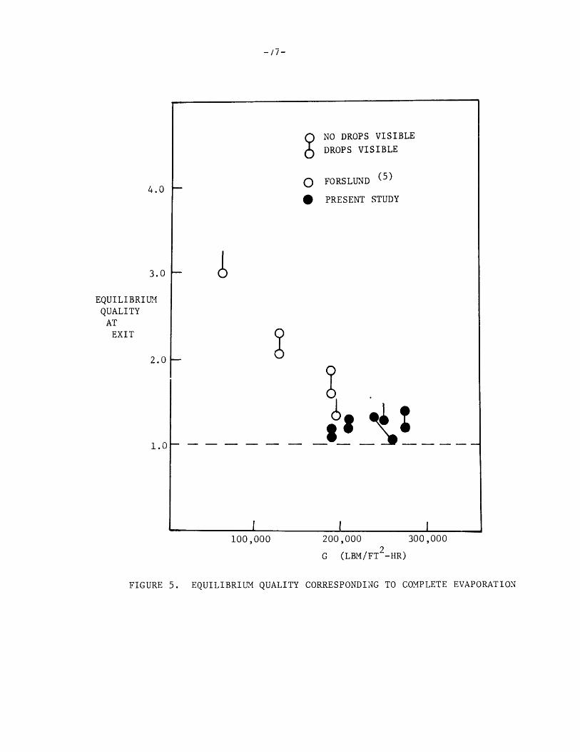
NO DROPS VISIBLE

DROPS VISIBLE

FORSLUND (5)

PRESENT STUDY4.0 t-

3.0 F-

EQUILIBRIUMQUALITYATEXIT

2.0

1.0

100,000 200,000 300,000

G (LBM/FT -HR)

FIGURE 5. EQUILIBRIUM QUALITY CORRESPONDING TO COMPLETE EVAPORATION

-'7-

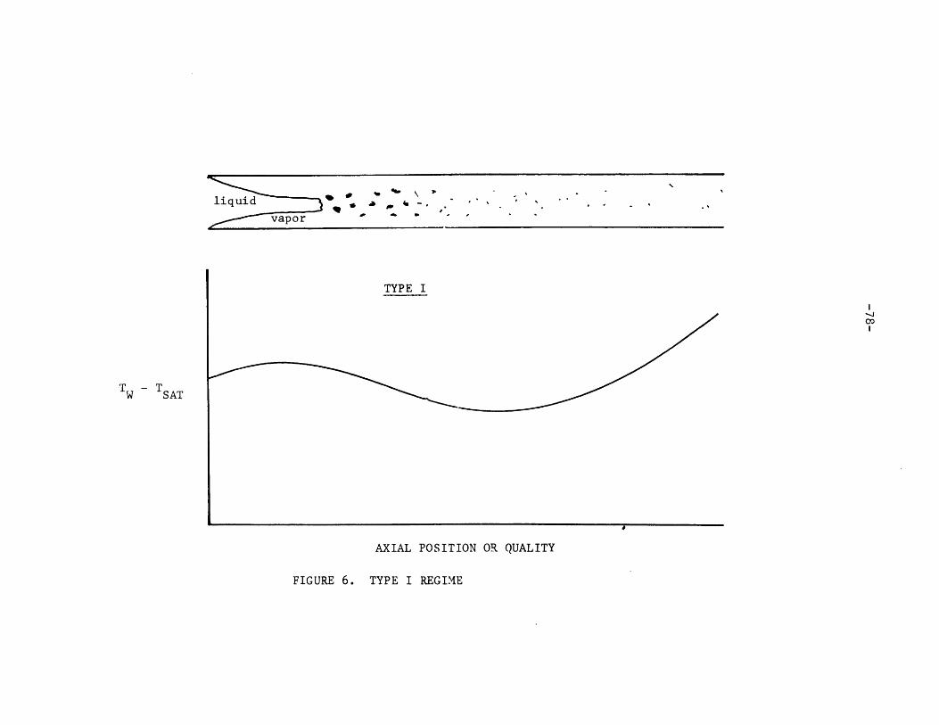
liquid -4-

vapor

TYPE I

0o

AXIAL POSITION OR QUALITY

FIGURE 6. TYPE I REGIME

W - TSAT

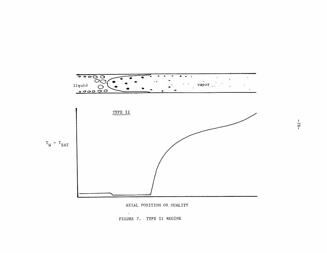
T TSAT

liquid - '' vapor-0~ 4w

TYPE II

AXIAL POSITION OR QUALITY

FIGURE 7. TYPE II REGIME

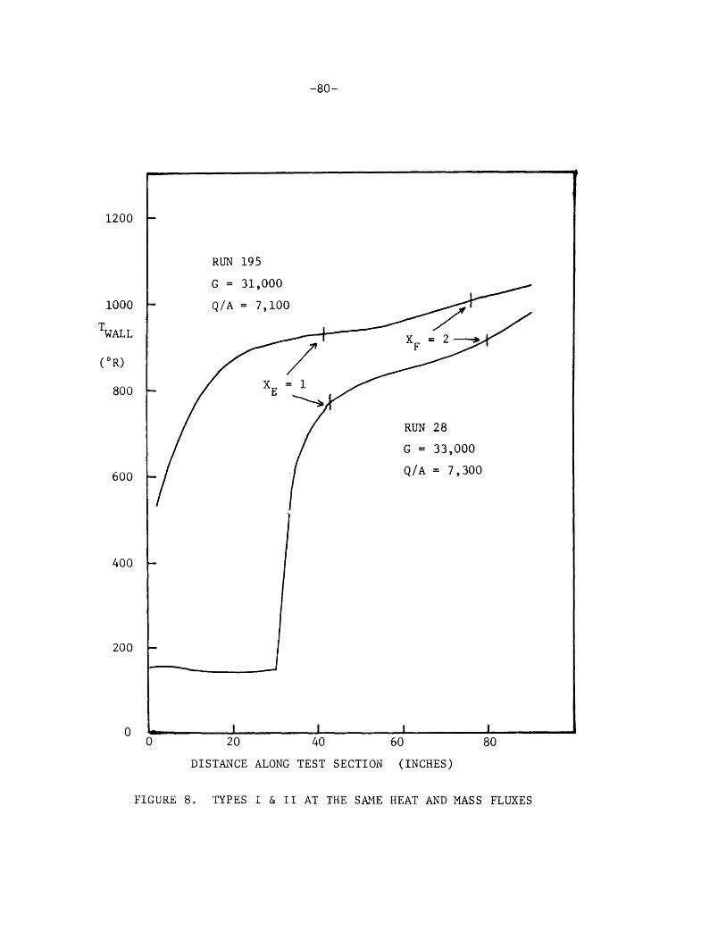
-80-

1200 -

RUN 195

G = 31,000

1000 - Q/A = 7,100

TWALL

(*R)

800 - XE

600 -

400 -

200 -

0 L0 20 40

DISTANCE ALONG TEST SECTION

FIGURE 8. TYPES I & II AT THE SAME HEAT AND MASS FLUXES

(INCHES)

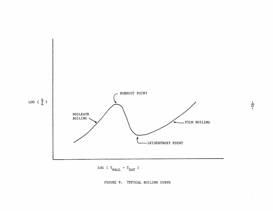
c BURNOUT POINT

'v - FILM BOILING

L-- LEIDENFROST POINT

LOG ( TWALL SAT

FIGURE 9. TYPICAL BOILING CURVE

LOG ( )

NUCLEATEBOILING

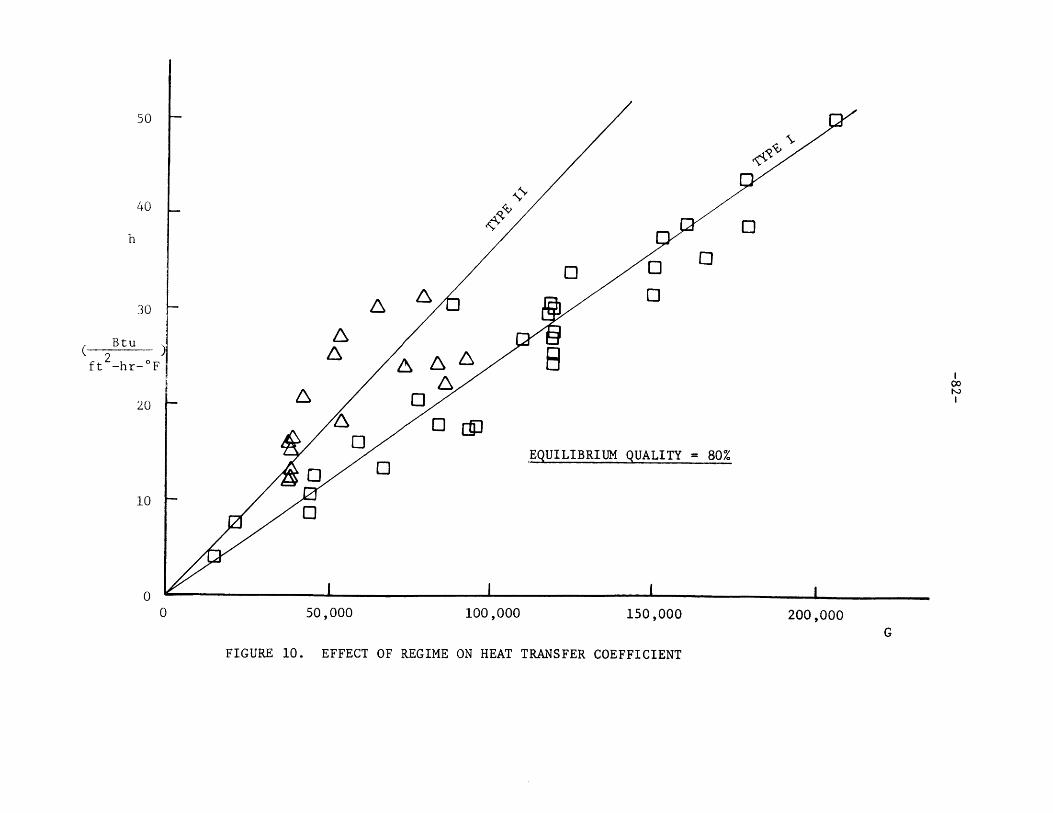
40 _

h

cl 0 0

30 -A A0

Btu Aft -hr-*F

20020 A 0l

0 EQUILIBRIUM QUALITY = 80%

10010 -

0 50,000 100,000 150,000 200,000

FIGURE 10. EFFECT OF REGIME ON HEAT TRANSFER COEFFICIENT

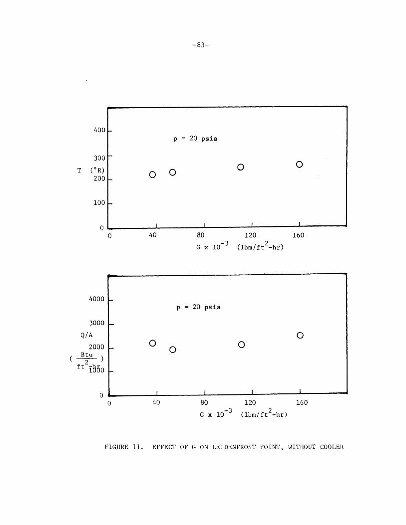
-83-

4001-

II

0 40 80 120 160

G x 10-3 (lbm/ft 2-hr)

p = 20 psia

-0 00 0

80 120

G x 10-3 (lbm/ft -hr)

160

FIGURE 11. EFFECT OF G ON LEIDENFROST POINT, WITHOUT COOLER

300

T (*R)200

00 1-.

p = 20 psia

00 0

0

4000

3000

Q/A

2000Btu - )ft 25b6o

0

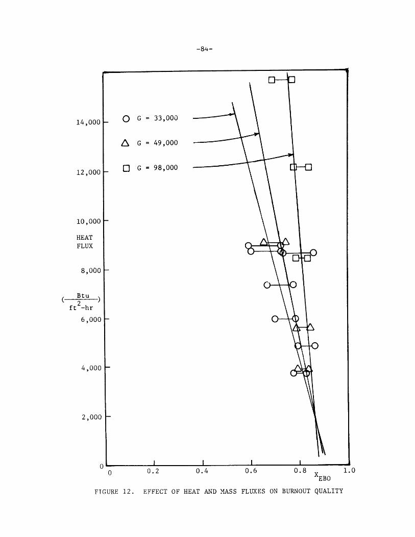
14,000 -

n 0.2

FIGURE 12. EFFECT OF HEAT AND MASS FLUXES ON BURNOUT QUALITY

-84-

o G = 33,000

A G = 49,000

o G = 98,00012,000 [-

10,000

HEATFLUX

,00 -

Btu

ft -hr

6,000

4,000 |-

2,000

0.4 0.6 0.8 XEBO

1.0

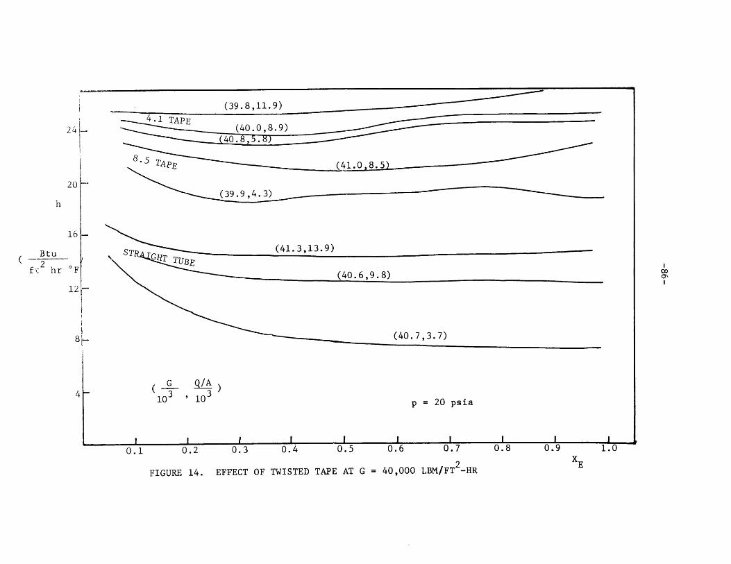
(39.8,11.9)4 . 1 TA P E (40 .0 98 .9 ) .............. ..... ........... ........... .

40.83,

8..5 7,A pe

Btu

f hr 0F

12-

81

G Q/A 10 3 ,10 3

0.1 0.2

p = 20 psia

0.3 0.4 0.5 0.b U. I ~L.U

FIGURE 14. EFFECT OF TWISTED TAPE AT G = 40,000 LBM/FT -HR

241

20

TRA ST(41.3,13.9)R4G 1 TUBE

0.6 0.7 0.8 I 0.9 i i

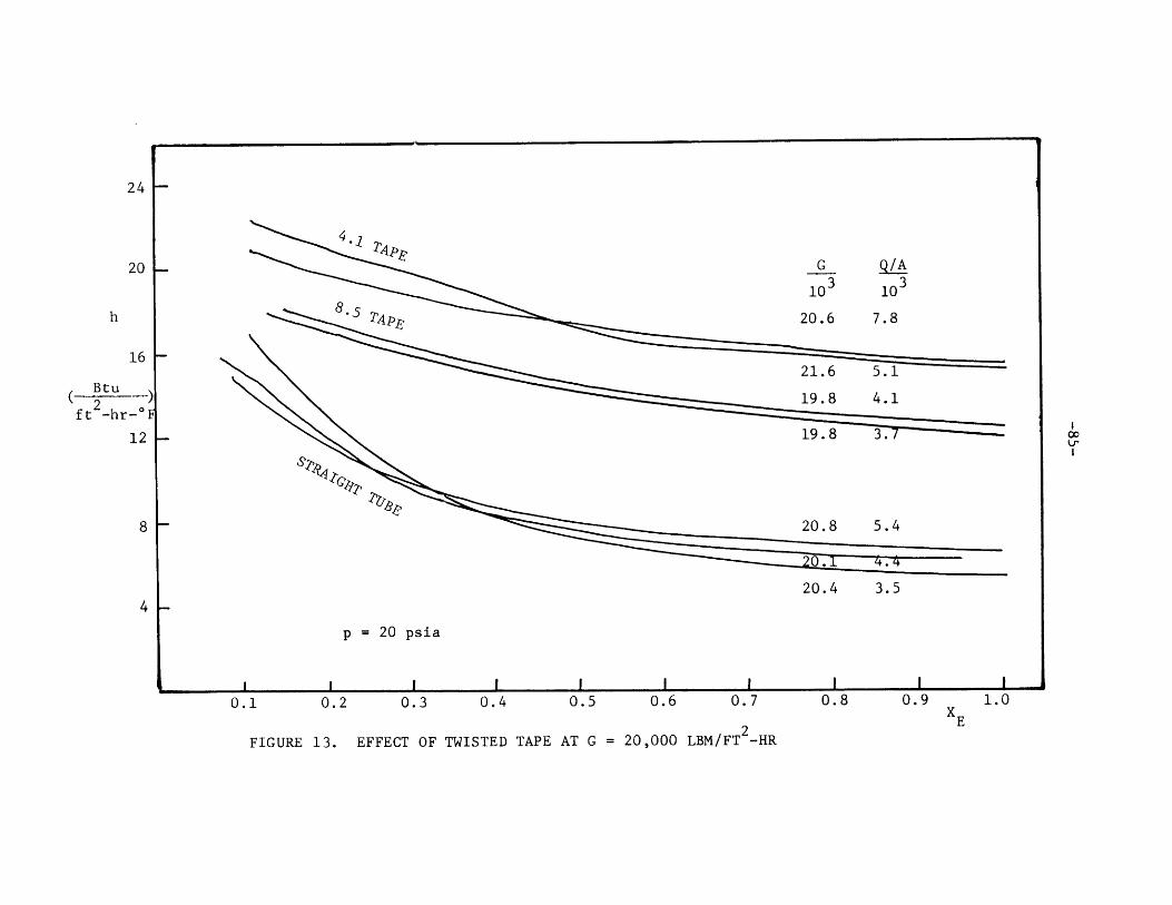
24 }-

20 -

16 }-

Btu

ft2 -hr-* F

12

8

420.4 3.5

p = 20 psia

0.2 0.3 0.4 0.5 0.6 0.7


0.1 0.8 0.9 1.0

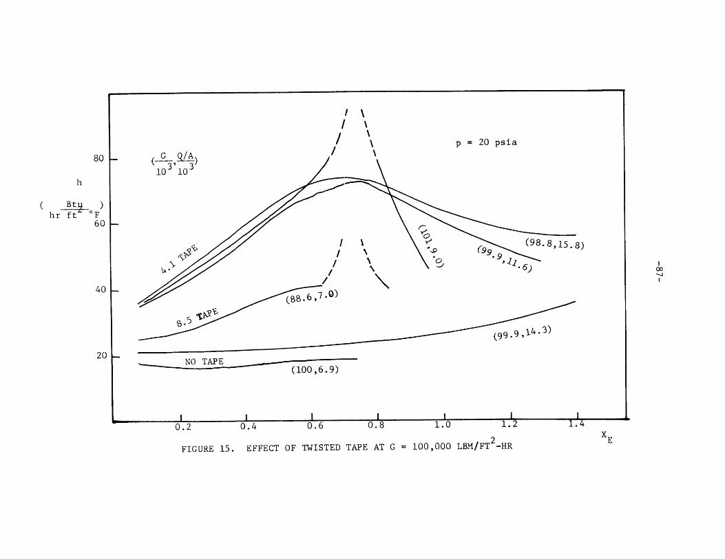
80 1-

h

(Btg )hr ft OF

60

p = 20 psia

G Q/A10 3103

40 1-.

20 ..

688. ,7

(99-914.3

NO TAPE(1003,6.9)

I 2 - 1 -~ 1 I.U.fj u.~j i.u j~.0.2 0.4


V- .Z I- . .L-.4I 1-0.6

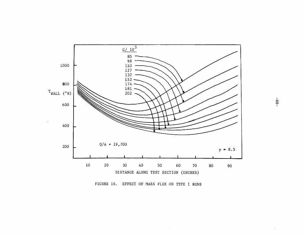
1000

800 174

T 181WALL (*R) 202

00

400.

200 Q/A = 19,700y = 8.5

10 20 30 40 50 60 70 80 90

DISTANCE ALONG TEST SECTION (INCHES)

FIGURE 16. EFFECT OF MASS FLUX ON TYPE I RUNS

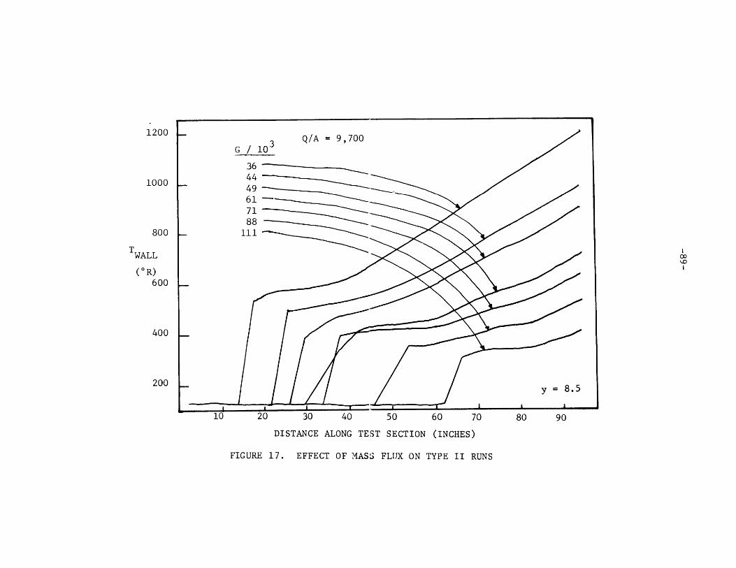
1200

1000

800

TWALL

(*R)600

400

200


FIGURE 17. EFFECT OF MASS FLUX ON TYPE II RUNS

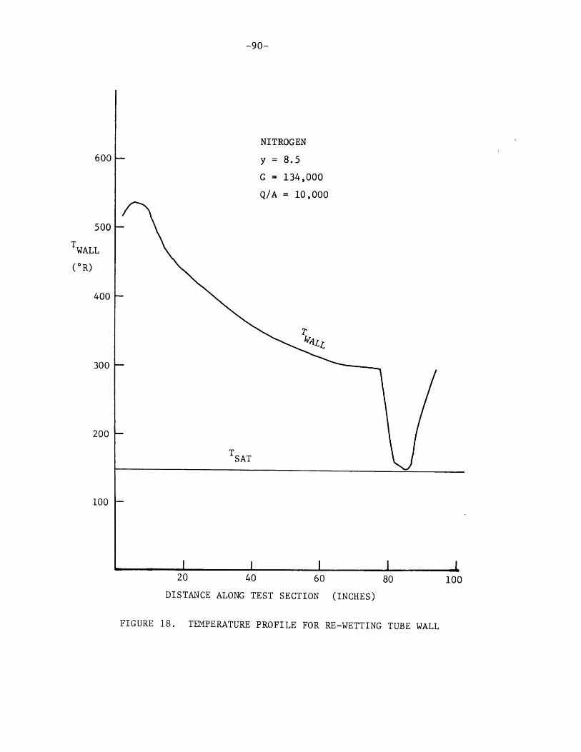
-90-

NITROGEN

600 - y = 8.5

G = 134,000

Q/A = 10,000

500 -

TWALL

(*R)

400 -

300 -

200 -

TSAT

100 -

I I I||20 40 60 80 100


FIGURE 18. TEMPERATURE PROFILE FOR RE-WETTING TUBE WALL

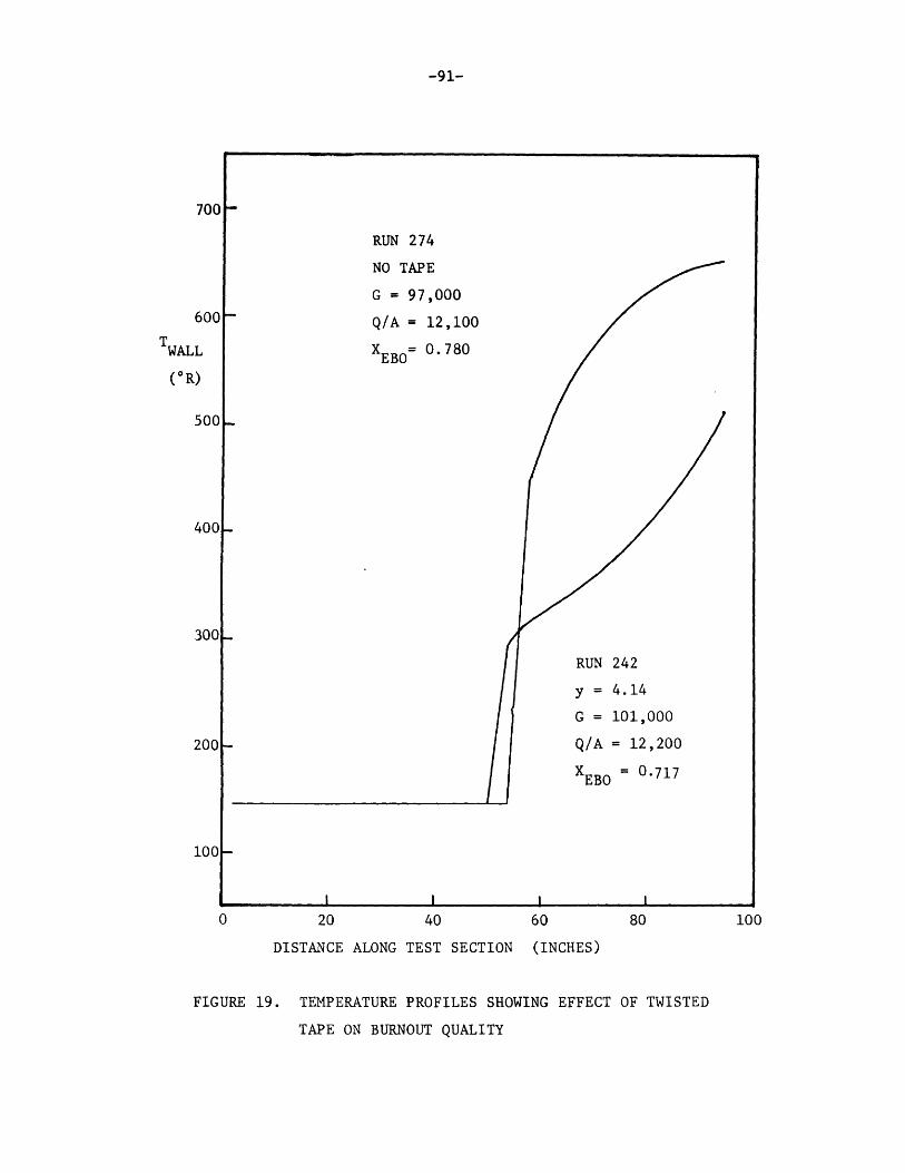
-91-

700F

RUN 274

NO TAPE

G = 97,000

Q/A = 12,100

XEBO 0.780

RUN 242

y = 4.14

G = 101,000

Q/A = 12,200

X EBO 0.717

20 40 60 80 100


FIGURE 19. TEMPERATURE PROFILES SHOWING EFFECT OF TWISTED

TAPE ON BURNOUT QUALITY

600

WALL

(0R)

500L-

4001.

300

200

100-

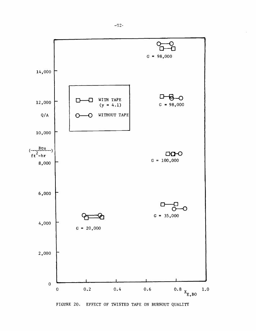
D-]0G = 98,000

G = 98,000

14,000

12,000

Q/A

10,000

Btu

ft -hr

8,000

6,000

0--OG = 35,000

G = 20,000

0.2 0.4 0.6 0.8 XEBO

FIGURE 20. EFFECT OF TWISTED TAPE ON BURNOUT QUALITY

WITH TAPE(y = 4.1)

Q- WITHOUT TAPE

G = 100,000

4,000

2,000

01.0

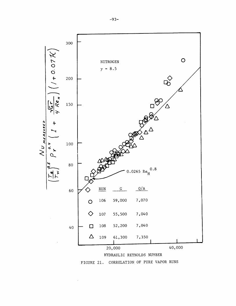
-93-

300

NITROGEN0

y = 8 . 5

1- 200

150

~loo100-

80

0.0265 ReH0

60 <> RUN G _Q/A_

o 106 59,000 7,070

107 55,500 7,040

40 Q 108 52,200 7,040

109 61,300 7,350

20,000

HYDRAULIC REYNOLDS NUMBER

FIGURE 21. CORRELATION OF PURE VAPOR RUNS

40,000

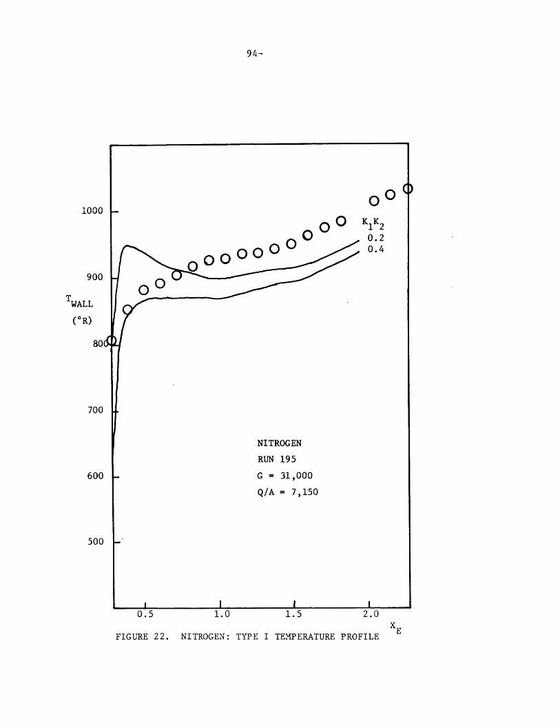
94.-

FIGURE 22. NITROGEN: TYPE I TEMPERATURE PROFILE

1000

900

TWALL

(*R)

801

700

600

500

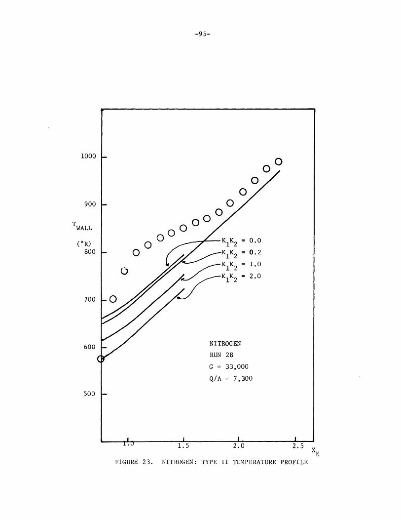
-95-

FIGURE 23. NITROGEN: TYPE II TEMPERATURE PROFILE

1000

900

TWALL

(*R)800

700

600

500

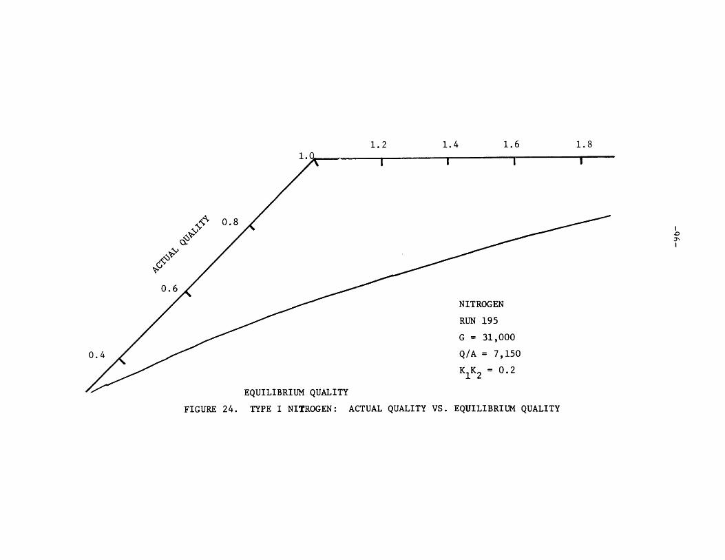
1.4 1.6 1.8

0.8

A4I

0.6

NITROGEN

RUN 195

G = 31,000

Q/A - 7,150

K1K = 0.2

EQUILIBRIUM QUALITY

FIGURE 24. TYPE I NITROGEN: ACTUAL QUALITY VS. EQUILIBRIUM QUALITY

0.4

1.2

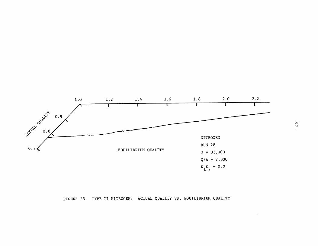
1.0 1.2 1.4 1.6 1.8 2.0 2.2

0.9

0.8

NITROGEN

RUN 280.7 EQUILIBRIUM QUALITY G = 33,000

Q/A = 7,300

K K2 0.2

FIGURE 25. TYPE II NITROGEN: ACTUAL QUALITY VS. EQUILIBRIUM QUALITY

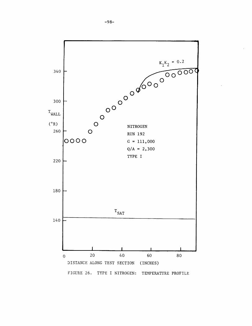
-98-

340

300 0 O

TWALL

(*R) 0 NITROGEN260 - 0 RUN 192

0000 G = 111,000

Q/A = 2,300

TYPE I220 -

180 -

TSAT

140 -

I -| I I

0 20 40 60


FIGURE 26. TYPE I NITROGEN: TEMPERATURE PROFILE

-99-

NITROGEN

RUN 194

G = 111,000

Q/A = 2,000

TYPE II00 0 0.

00 1 1 g 0.2

300 - i2

T WALL 0

(*R)

260

220 -

180 -

00000 0 O O 0 TSAT140 -

I I I I I0 20 40 60 80


FIGURE 27. TYPE II NITROGEN: TEMPERATURE PROFILE

340

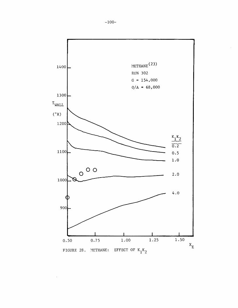
-100-

0.75 1.00 1.25 1.50

METHANE: EFFECT OF K K1 K2

1400

1300

TWALL

(*R)

1201

110'

0.50

FIGURE 28.

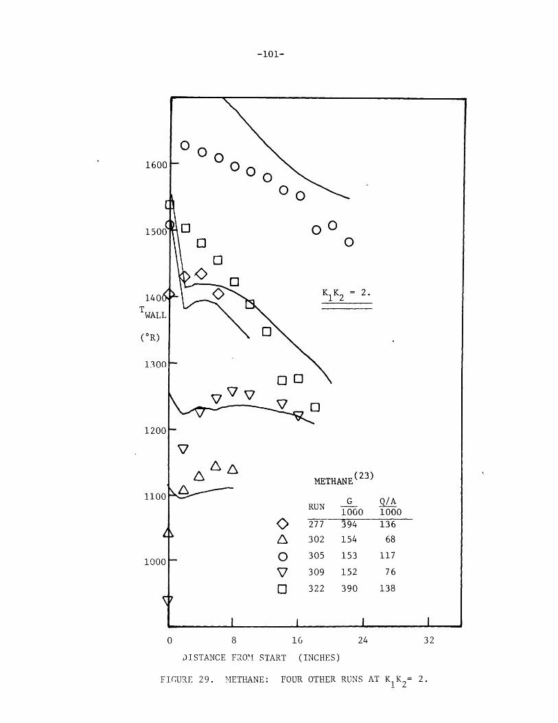
-101-

0 8 16 24 32

DISTANCE FROM1 START (INCHES)

FIGURE 29. METHANE: FOUR OTHER RUNS AT KK 2= 2.

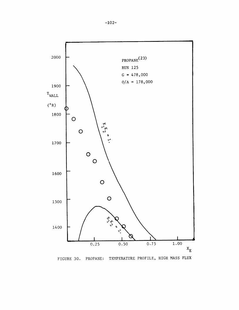
-102-

2000

1900

TW1ALL

(*R)

1800

1700

1600

1500

1400

0.25 0.50 0.75 1.00

FIGURE 30. PROPANE: TEMPERATURE PROFILE, HIGH MASS FLUX

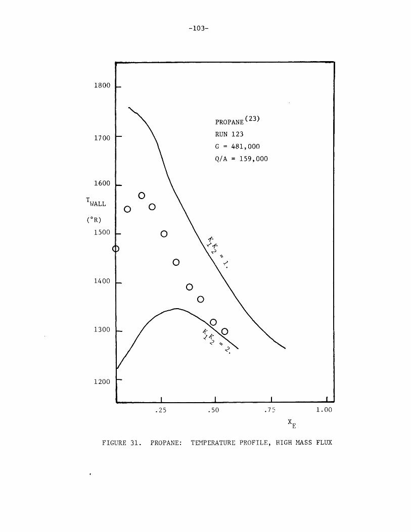
-103-

.25 .50 .75 1.00

FIGURE 31. PROPANE: TEMPERATURE PROFILE, HIGH MASS FLUX

1800

1700

1600

TW1ALL

(*R)

1500

1400

1300

1200

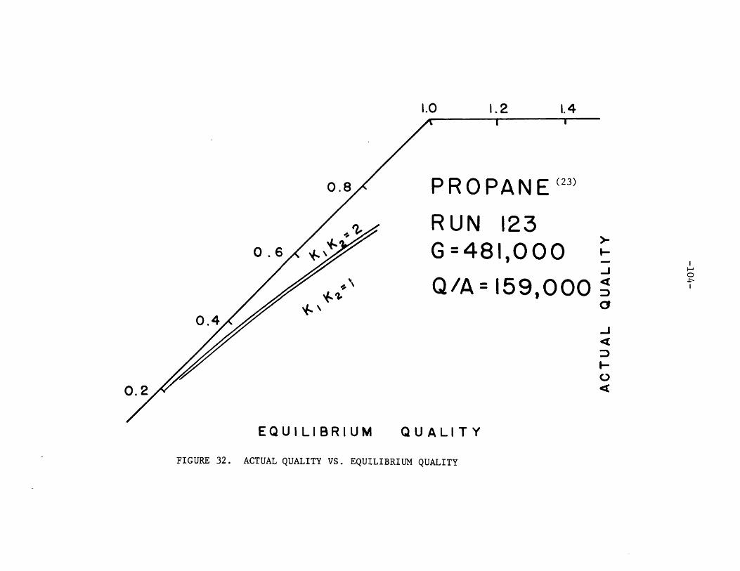
1.2

0.8

0.6

0.4

0.2

EQUILIBRIUM QU A LI T Y

FIGURE 32. ACTUAL QUALITY VS. EQUILIBRIUM QUALITY

PROPANE"2

RUN 123G=481,000

Q/A = 159,000

1.0 1.4

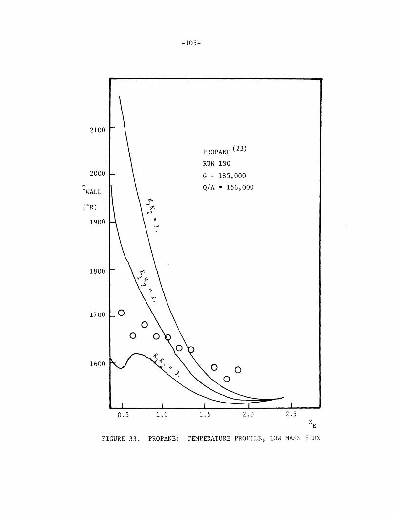
-105-

2100

2000

TWALL

(*R)

1900

1800

1700

1600

0.5

FIGURE 33.

1.0 1.5 2.0 2.5XE

PROPANE: TEMPERATURE PROFILE, LOW MASS FLUX

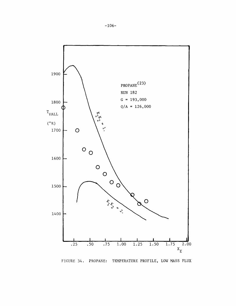
-106-

1900-

PROPANE (23)

RUN 182

1800 G = 193,000

( Q/A = 126,000

T WALL

(*R)

1700 -

1600 -

00

1500 - O

1400

, I I I II i{.25 .50 .75 1.00 1.25 1.50 1.75 2.00

XE

PROPANE: TEMPERATURE PROFILE, LOW MASS FLUXFIGURE 34.

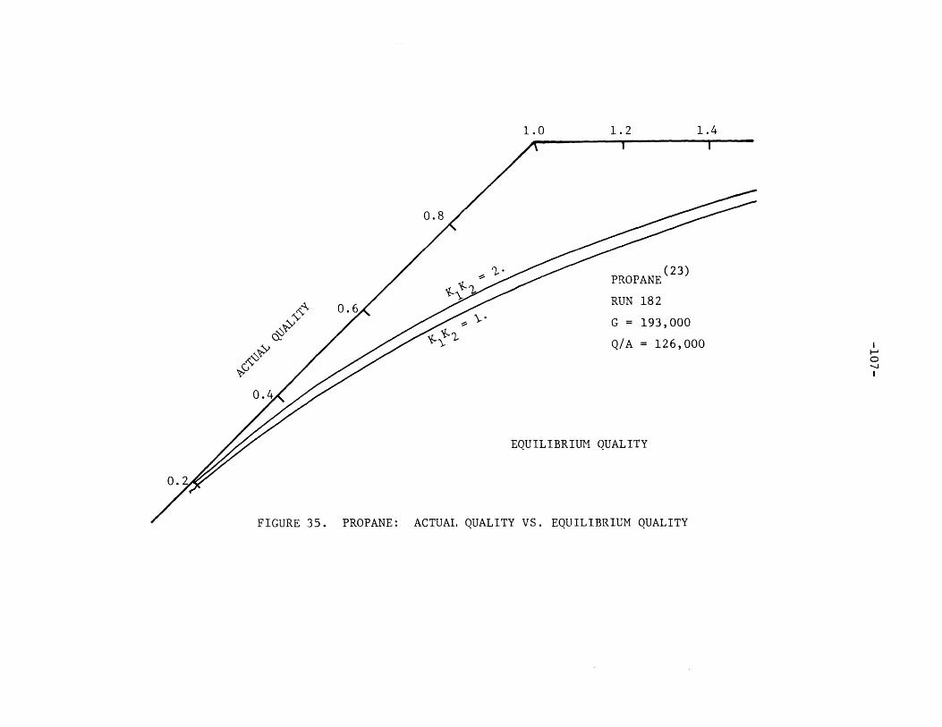
1.0 1.2

0.8

PROPANE(2

RUN 182

G = 193,000

Q/A = 126,000

EQUILIBRIUM QUALITY

FIGURE 35. PROPANE: ACTUAL QUALITY VS. EQUILIBRIUM QUALITY

-V

1.4

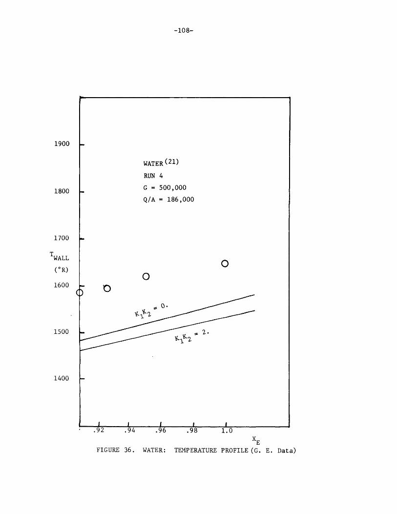
-108-

FIGURE 36. WATER: TEMPERATURE PROFILE (G. E. Data)

1900

1800

1700

TWALL

(*R)

1600

1500

1400

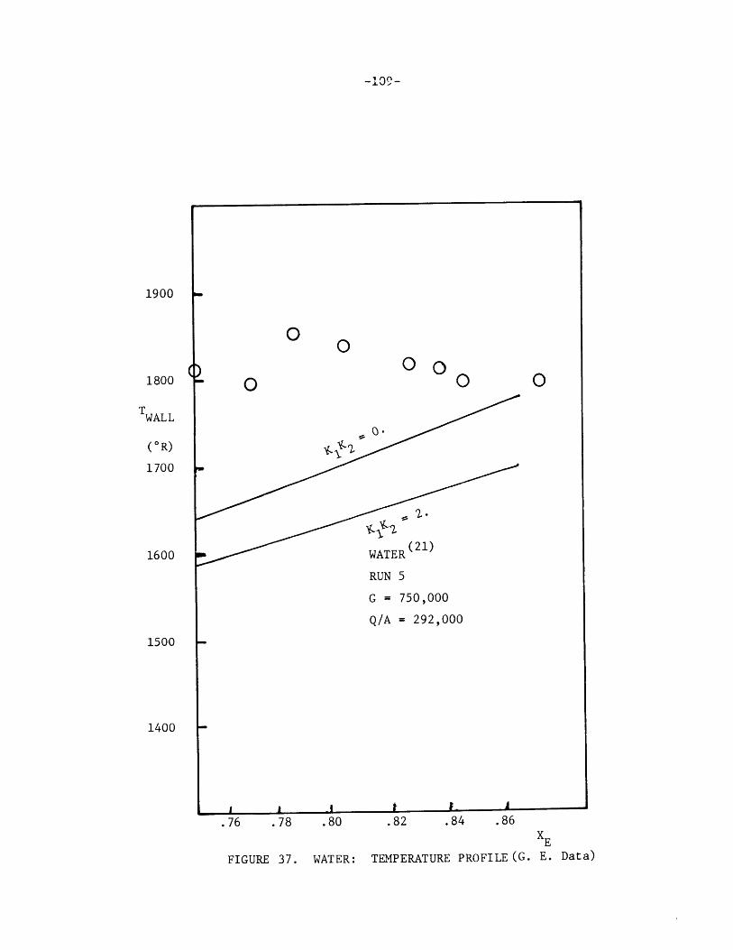
-10%

.76 .78 .80 .82 .84 .86

WATER: TEMPERATURE PROFILE (G. E. Data)

1900

1800

TWALL

(*R)

1700

1600

1500

1400

FIGURE 37.

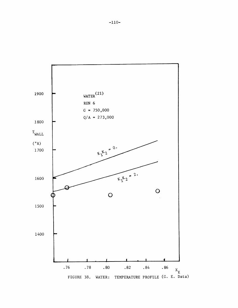
-110-

.76 .78 .80 .82 .84 .86

WATER: TEMPERATURE PROFILE (G. E. Data)

1900

1800

TWALL

(*R)

1700

1600

1500

1400

FIGURE 38.

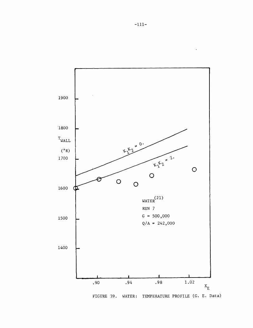
-111-

.90 .94 .98 1.02

FIGURE 39. WATER: TEMPERATURE PROFILE (G. E. Data)

1900

1800

TWALL

(*R)

1700

1600

1500

1400

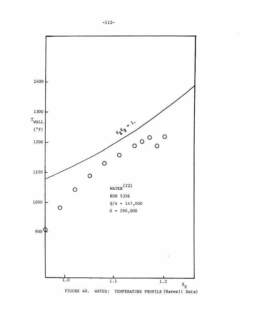
-112-

1.1 1.2

WATER: TEMPERATURE PROFILE (Harwell Data)

1400

1300

TWALL

(*F)

1200

1100

1000

900

FIGURE 40.

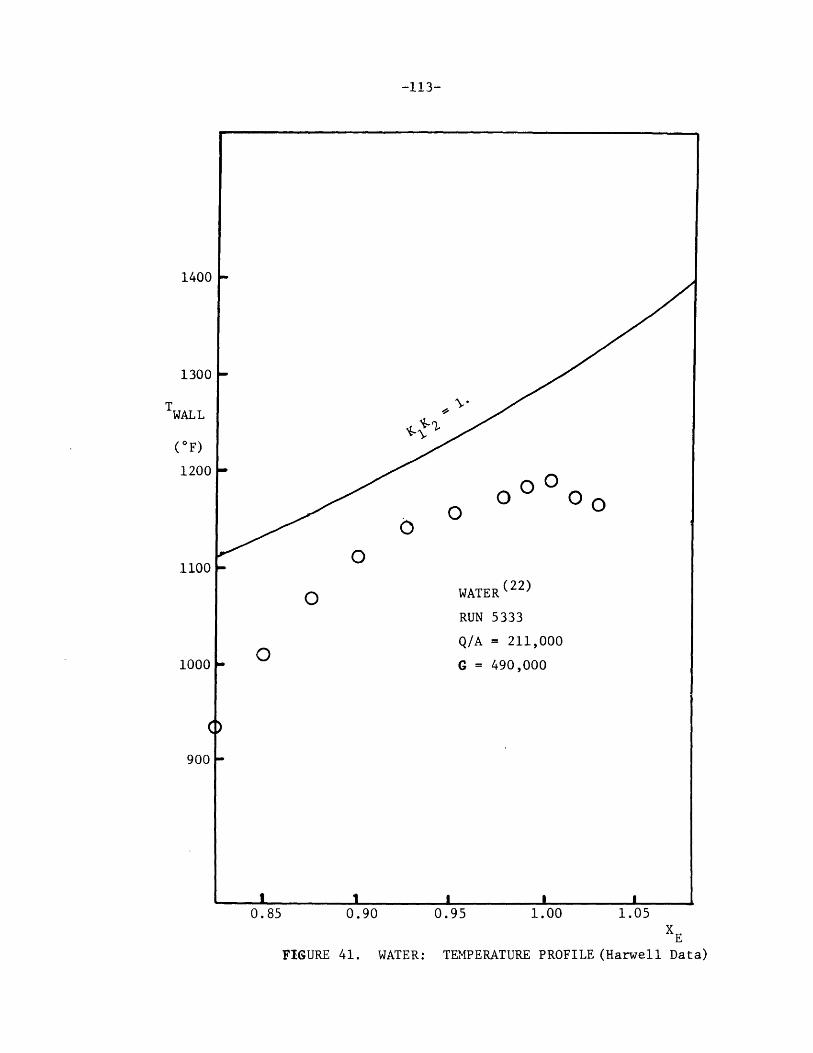
-113-

0.90 0.95 1.00 1.05

FIGURE 41. WATER: TEMPERATURE PROFILE (Harwell Data)

1400

1300

TWALL

(*F)

1200

1100

1000

C

900

0.85

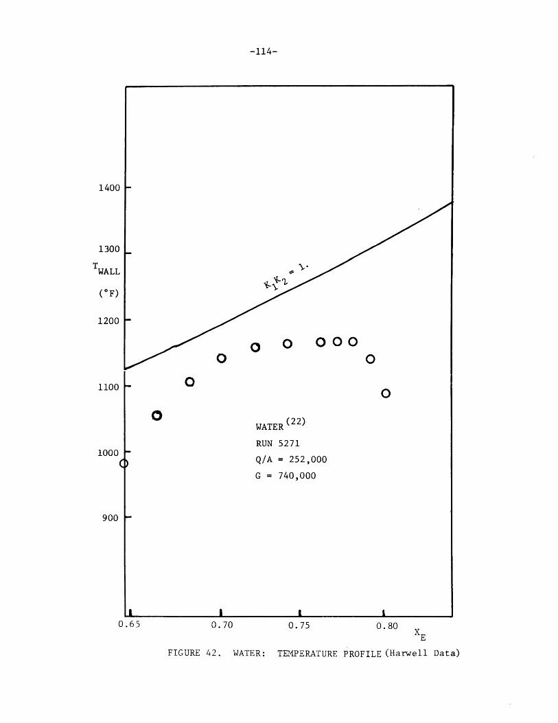
-114-

1400

1300

TWALL

(*F)

1200

O 0

1100 0 0

WATER (22)

RUN 5271

Q/A = 252,000

G = 740,000

900 -

0.65 0.70 0.75 0.80

TEMPERATURE PROFILE (Harwell Data)FIGURE 42. WATER:

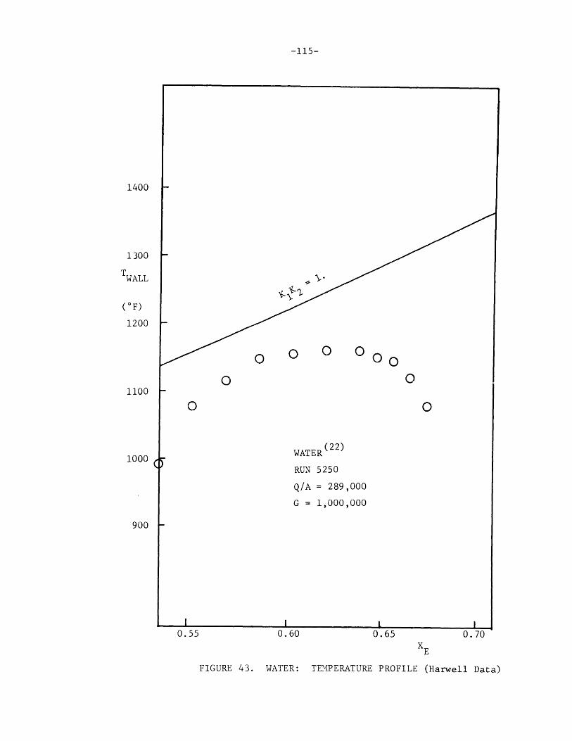
-115-

0.55 0.60 0.65 0.70

WATER: TEMPERATURE PROFILE (Harwell Data)

1400

1300

TWALL

(*F)

1200

1100

1000

900

FIGURE 43.

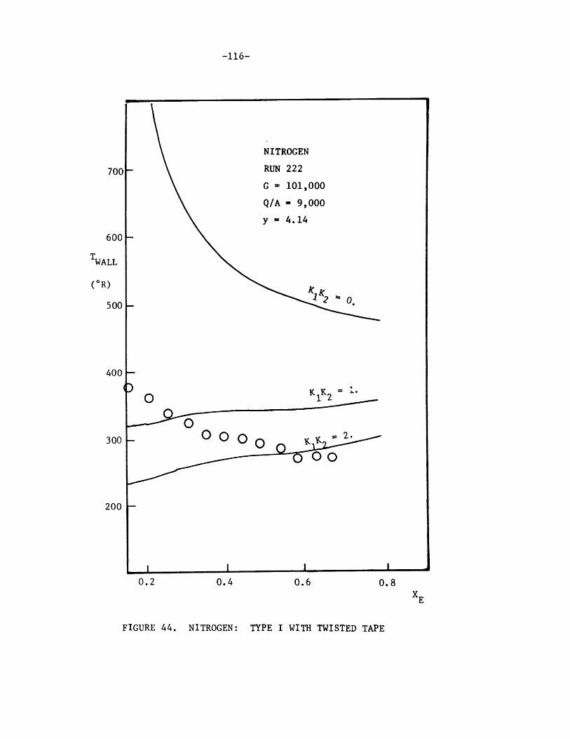
-116-

7001

600

TWALL

(*R)

500

400

300

200

0.2 0.4 0.6 0.8

FIGURE 44. NITROGEN: TYPE I WITH TWISTED TAPE

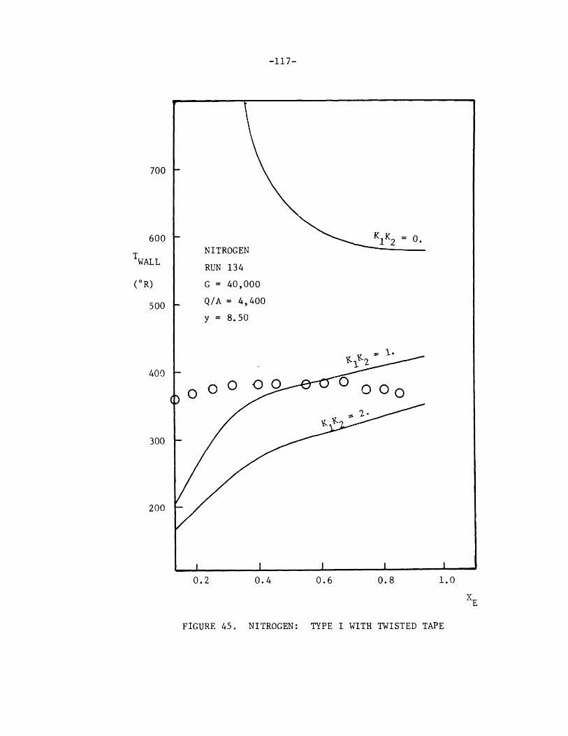
-117-

0.2 0.4 0.6 0.8 1.0

FIGURE 45. NITROGEN: TYPE I WITH TWISTED TAPE

700

600

TWALL

(*R)

500

400

300

200

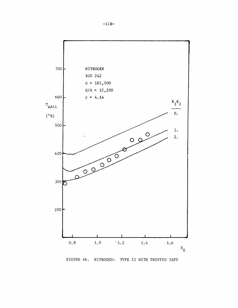
-118-

1.0 -1.2 1.4 1.6

NITROGEN: TYPE II WITH TWISTED TAPE

700

600

TWALL

(*R)

500

400

300

200

0.8

FIGURE 46.

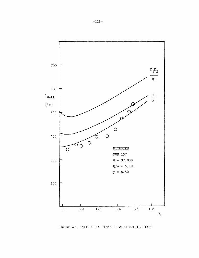
-119-

1.0 1.2 1.4 1.6 1.8

FIGURE 47. NITROGEN: TYPE II WITH TWISTED TAPE

700

600

TWALL

(*R)

500

400

300

200

0.8

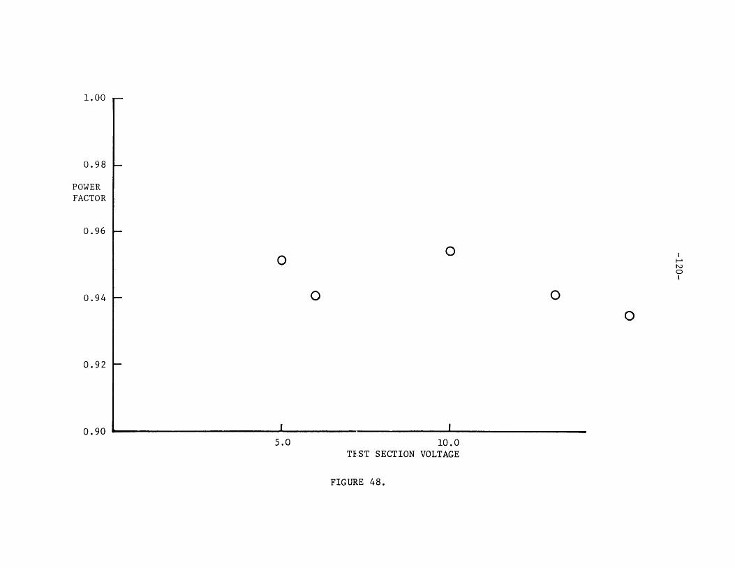
1.00 r-

0.98 -

POWERFACTOR

0.96 -

00

0.92 -

0.90 L5.0 10.0

TEST SECTION VOLTAGE

FIGURE 48.

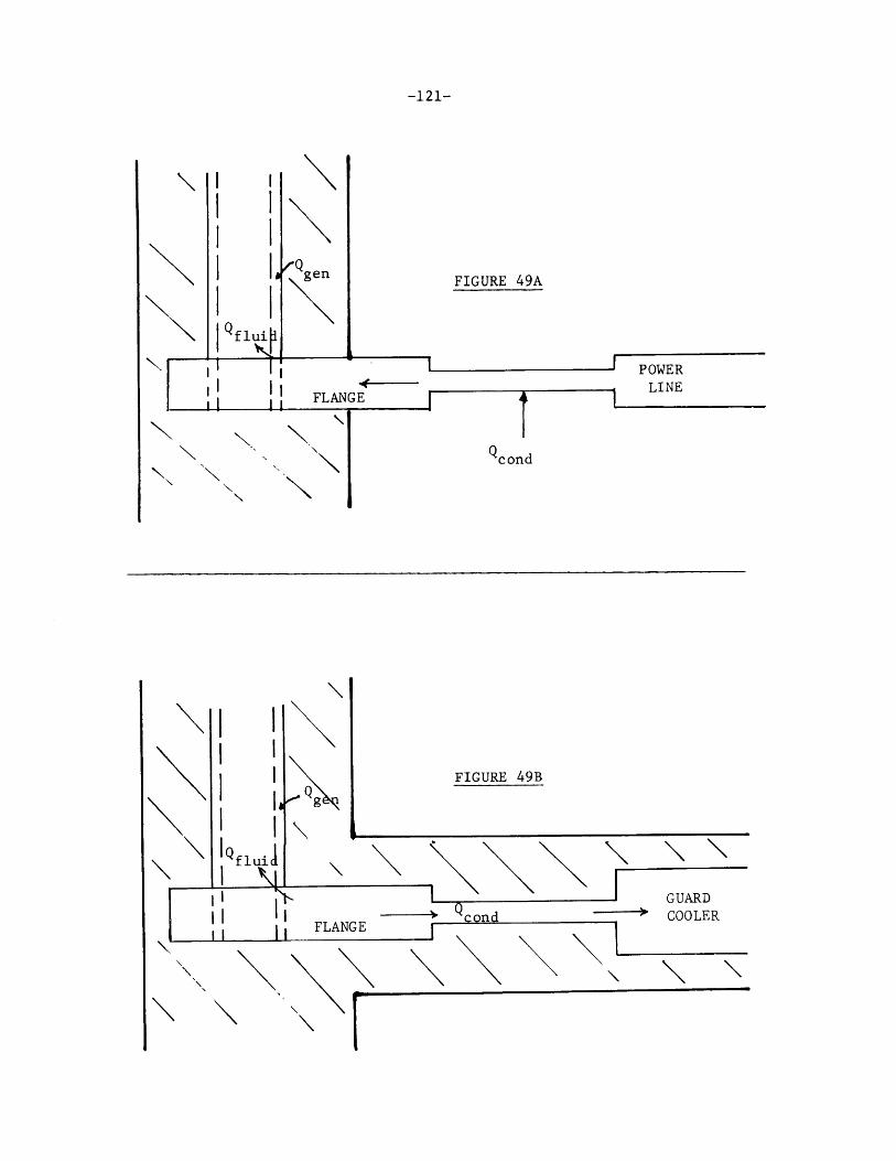
FLANGE

K

FIGURE 49AI,

Qf lui

FIGURE 49B

GUARD

SE cond COOLER

-121-

'egen

POWERLINE

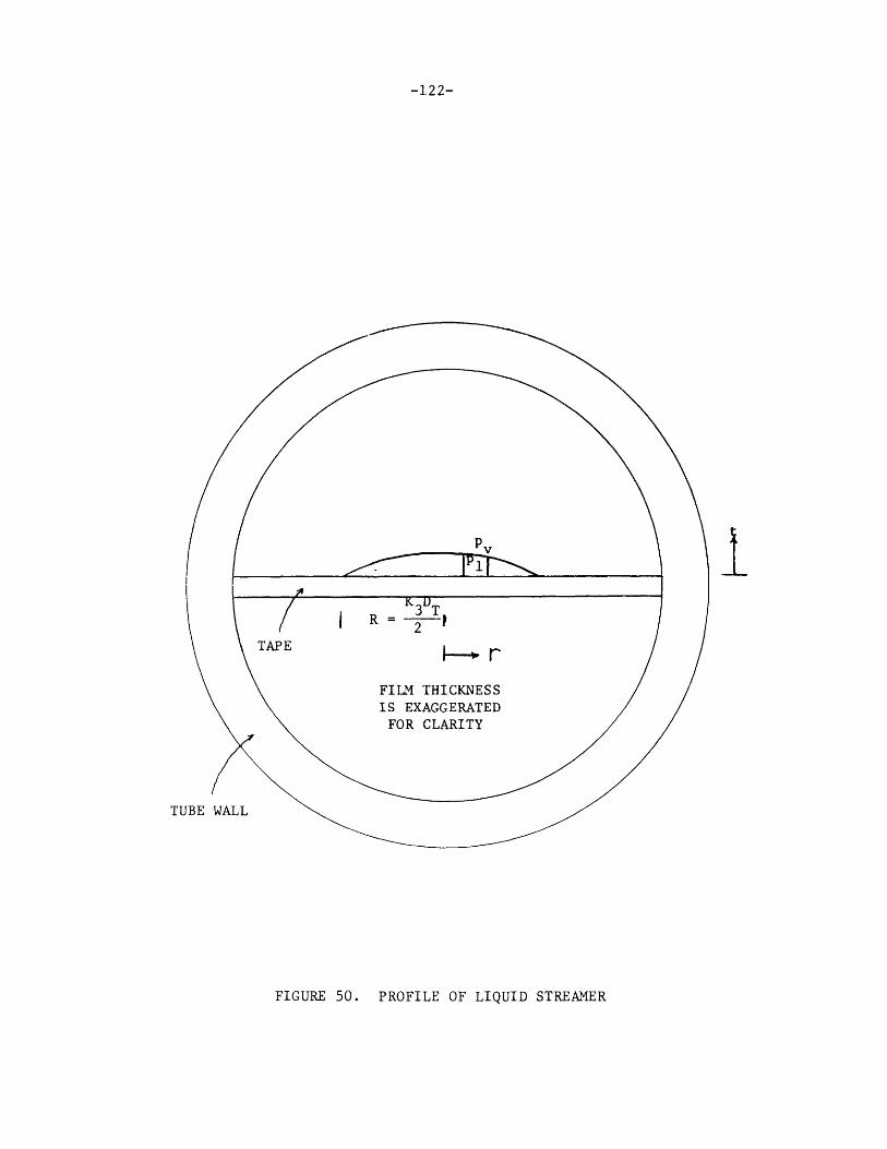
-122-

I

PROFILE OF LIQUID STREAMERFIGURE 50.

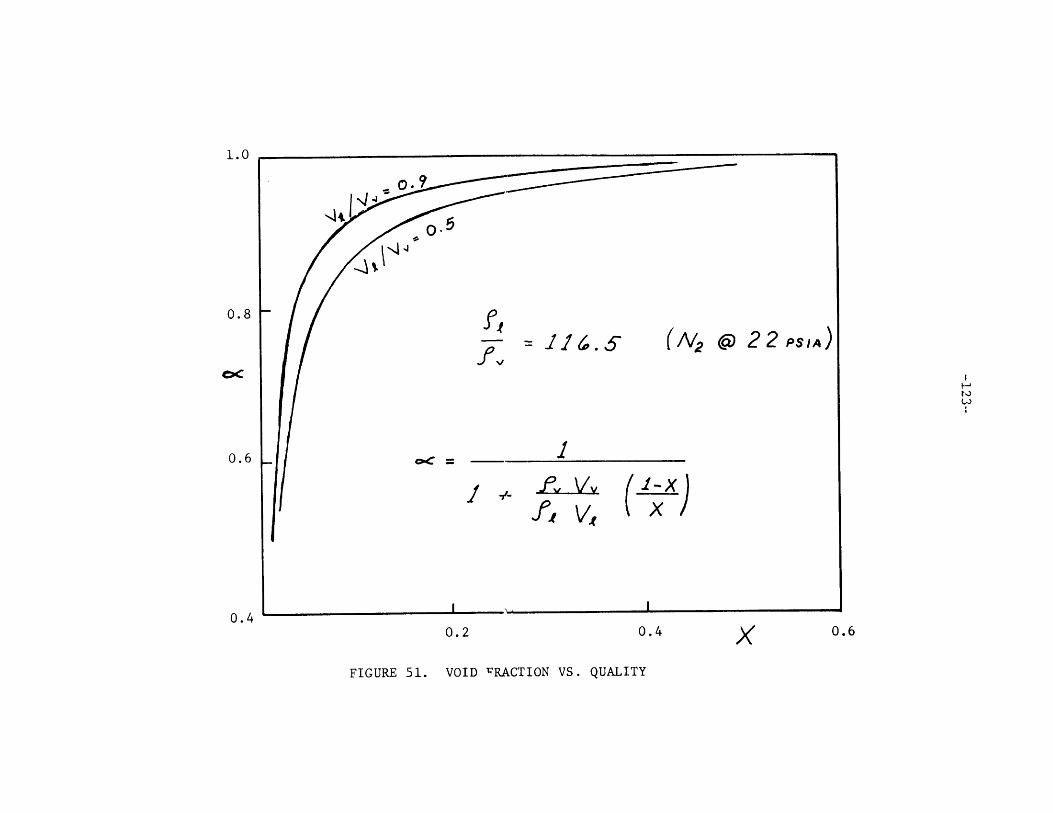
(V2 @ 22 PSIA)

-xfv V.

0.2 0.4

FIGURE 51. VOID VRACTION VS. QUALITY

v,44

1.0

0.8

0.6

ft

og =

0.4

x 0.6

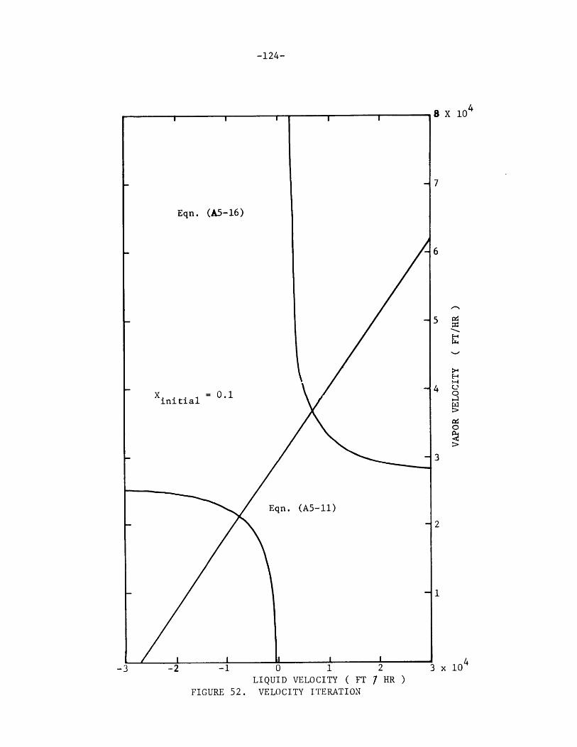
-124-

8 x 10

-6

0.10

3

Eqn. (A5-ll)

2

-- 4

-1 0 1 2 3 x 10

LIQUID VELOCITY ( FT HRFIGURE 52. VELOCITY ITERATION

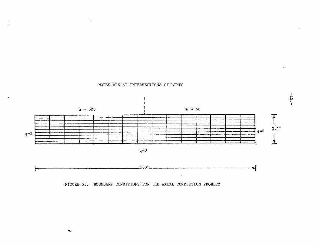
NODES ARE AT INTERSECTIONS OF LINES

q=0

*1 ()If

FIGURE 53. BOUNDARY CONDITIONS FOR THE AXIAL CONDUCTION PROBLEM

h = 500

q=O

h = 50

Tq= 0.1"

L

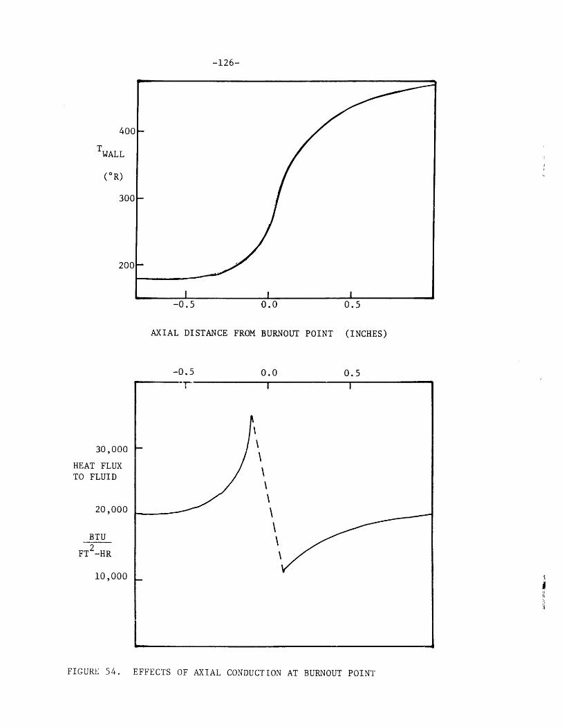
TWALL

(*R)

-0.5 0.0 0.5

AXIAL DISTANCE FROM BURNOUT POINT (INCHES)

-0.5

30,000

HEAT FLUXTO FLUID

20,000

BTU

FT -HR

10,000

FIGURE 54. EFFECTS OF AXIAL CONDUCTION AT BURNOUT POINT

-126-

0.0 0.5

FORCED -CONVECTION DISPERSED-

Documents

Transcript of FORCED -CONVECTION DISPERSED-