For Rich or for Poor: When does Uncovered Interest Parity Hold?

Michael J. Moore*

Queen’s University, Belfast, Northern Ireland

Maurice J. Roche

Ryerson University, Toronto, Canada

This version: 17th

December 2009

Abstract

We present a model that simultaneously explains why uncovered interest parity holds for some

pairs of countries and not for others. The flexible-price two-country monetary model is

extended to include a consumption externality with habit persistence. Habit persistence is

modeled using Campbell Cochrane preferences with ‘deep’ habits along the lines of the work of

Ravn, Schmitt-Grohe and Uribe. By deep habits, we mean habits defined over goods rather than

countries. The negative slope in the Fama regression arises when monetary instability is low and

the precautionary savings motive dominates the intertemporal substitution motive. When

monetary instability is high, the Fama slope is positive in line with uncovered interest parity.

The model is simulated using the artificial economy methodology for 34 currencies against the

US dollar. We conclude that, given the predominance of precautionary savings, the degree of

monetary instability explains whether or not uncovered interest parity holds.

Keywords: Monetary instability; Uncovered interest parity; Forward biasedness puzzle; Carry

trade; Habit persistence

JEL classification: F31; F41; G12

*The address for correspondence is

Michael J. Moore,

Queen's University Management School,

Queen’s University, Belfast,

Belfast BT7 1NN, Northern Ireland.

Tel/Fax +44 (0) 28 90973208; email m.moore@qub.ac.uk

Moore thanks the UK Economic and Social Science Research Council for support under grant number RES-000-22-

2177. Roche thanks the Irish Research Council for the Humanities and Social Sciences for support under

Government of Ireland’s Thematic Research Project Grants Bi-Lateral Scheme 2006-07. We thank Menzie Chinn,

Bob Dittmar and Martin Evans for helpful comments.

1

1. Introduction.

Eichenbaum (2008) investigates equally weighted carry trade portfolios for 20 portfolios

over a thirty year period and finds consistent excess dollar returns. A ‘carry trade portfolio’ is a

strategy of borrowing in the currency of the low interest currency and depositing the proceeds in

the high interest currency, taking an open position to nominal exchange rate risk. He concludes

that this vividly demonstrates the pervasiveness of the forward ‘bias’ puzzle. The contribution of

this study is to specify and test a theory which provides for when the forward bias does and does

not hold.

The literature that studies this puzzle or equivalently the failure of uncovered interest

parity (UIP) is enormous. The classic survey is Engel (1996) and Sarno (2005) contains a good

update. There is a multitude of relatively recent theoretical papers which explain the failure of

uncovered interest parity. There are behavioural explanations (Burnside, Eichenbaum and

Rebelo, 2007, Fisher, 2006 and Gourinchas and Tornell, 2004); rational inattention is offered by

Bachetta and Van Wincoop (2008); institutional features are emphasised by Carlson and Osler

(2005); and Alvarez, Atkinson and Kehoe (2006) explain the forward bias by permitting a time

varying degree of asset market participation. Bansal and Shaliastovich (2007) extend the Bansal

and Yaron (2004) model to explain the forward bias using Epstein-Zin preferences, long-run

growth fluctuations and time-varying uncertainty. In a model related to the one explored in this

paper, Verdelhan (2010) attempts to explain the forward bias puzzle using Campbell and

Cochrane (1999) preferences in a non-monetary economy with trade costs. It is difficult to

interpret this work because real interest rates cannot be observed so that it is not clear if there is a

real analogue to the forward bias problem in the data. Moore and Roche (2007) show that the

2

Verdelhan (2010) result can be obtained as a special case of our analysis, without the contrivance

of trade costs.

A different line of empirical research has suggested that the forward bias problem does

not always occur. Chinn (2006) provides a good review of cases where UIP does hold1. Our

main focus is on the claim that the forward bias problem is a feature which arises between

developed countries and is much less likely to arise between emerging and developed countries.

This was first suggested by Bansal2 and Dahlquist (2000). Frankel and Poonawala (2009), Chinn

(2006) as well as Ito and Chinn (2007) find similar results. Flood and Rose (2002) buck the

trend by finding no significant difference in the success of UIP between rich and poor countries.

Most interestingly, they find that UIP works systematically better for ‘crisis’ countries. This is

the starting point for this paper.

Our modelling strategy is to extend Campbell and Cochrane (1999) preferences to both a

monetary and an international setting along the lines of Moore and Roche (2002, 2005, 2007,

2008). With this specification there is an aggregate consumption externality (see for example

Abel (1990) and Duesenberry (1949)) and utility is time-inseparable because of habit

persistence. The utility function depends not only on the consumption of domestic and foreign

endowments but also on the surplus of consumption over externally generated volatile and

persistent habits, in each good. Ravn, Schmitt-Grohe, and Uribe (2006, 2007) refer to this

preference specification as “deep habit formation”. In the standard model, when the domestic

interest rate is relatively low, the exchange rate is expected to appreciate. The forward bias in

1 Chinn and Meredith (2004) show that UIP is mainly violated for short maturity bonds. For longer maturity bonds,

the negative coefficient does not arise and is closer to one than zero. Alexius (2001) finds a similar result. We do

not pursue this feature in this study though the violation of uncovered interest parity is only a short-run problem in

the framework that we present. 2 Curiously, they make no attempt to explain the divergent results of Bansal and Dahlquist (2000). It is surprising

that Bansal does not address his empirical results in his 2007 theoretical paper with Shaliastovich. This is almost

certainly due to the fact that their model is cast in terms of real variables: they characterize nominal magnitudes by

bolting on an exogenous forcing process for inflation, as an afterthought.

3

our model arises because the preference specification has two motives for savings. The first is

the conventional desire to smooth consumption intertemporally. The less familiar motive is a

precautionary savings effect, which is dominant in our calibration of the model. When times are

relatively bad for the owner of the domestic endowment, the surplus consumption ratio for the

domestic good is low in relation to that for the foreign good, the time-varying risk aversion

measured in the domestic good is relatively high and the own interest rate is relatively low.

Consequently the holder of the domestic bond does not need to be compensated by as much of an

expected appreciation and indeed may be content with an expected depreciation. The latter case,

which arises easily in our model, is why the forward bias can occur.

The above argument is apparently so compelling that it begs the question as to why UIP

would ever hold at all. The answer to this is that the argument in its extreme form applies to a

world without nominal magnitudes. We show that when these are built into agents’ optimising

model, the above result can be reversed. We show that an increase in monetary instability

requires that nominal interest rates be raised to compensate the holder of nominal bonds. Our

model identifies monetary instability with the conditional variance of monetary growth. Note

how precise this point is: we are not considering first moments such as money growth or

inflation but a second moment: the stability of monetary policy. Whether or not UIP holds is a

balance between the extent of monetary instability and the dominance of the real precautionary

savings motive.

It is easy to see how the failure or otherwise of UIP might follow developed/emerging

economy lines. Emerging economies are far more likely to be characterised by unstable

monetary regimes and therefore UIP is more likely to hold. The opposite is obviously true of

developed countries.

4

The plan of the paper is as follows. In the next section, the model is outlined. Section 3

is the substantial contribution of the paper in which the model is calibrated and the results are

reported. Section 4 makes some concluding remarks.

2. The Model

2.1 Basic Framework

We extend the Campbell and Cochrane (1999) to an international and monetary setting. A

two-country, two-good, two-money representative agent model is developed similar to that of

Lucas (1982). The markets for state-contingent money claims are made complete by having one

period contingent nominal bonds as in Chari, Kehoe and McGrattan (2002).

The household in country 1 is assumed to choose consumption of goods and services of

country j, 1

j

tC , to purchase state contingent nominal bonds 1

1( )tB τ + (each of which pays off one

unit of home currency in state 1tτ + ) and

2

1( )tB τ + (each of which pays off one unit of foreign

currency in state 1tτ + ) to maximize the following expected discounted lifetime utility function

3:

1 1 (1 ) 2 2 (1 )

1 1 1 1

0

( ) ( )

1 1

t t t t tt

t

C H C HE

γ γ

βγ γ

− −∞

=

− −+

− − ∑ (1)

subject to the equation of motion for wealth in country 1, 1

1tW + :

1 1

1 1 2 1 1

1 1 1 1( ) ( )t t

t t t t t tW B S B P Yτ τ

τ τ+ +

+ + + +∈Τ ∈Τ

= + +∑ ∑ (2)

and the wealth constraint:

3 The superscript denotes country of origin of the good. Uppercase letters denote variables in levels; lowercase

letters denote variables in log levels, including growth and interest rates. Greek letters without time subscripts

denote parameters. Bars over variables denote steady states. With the exception of the money growth process

discussed below, we assume that the parameters in the model are identical for both countries. This is not essential to

the model but we have not found it necessary to emphasize cross-country parameter differences. Because of this and

for simplicity of exposition, we present the problem for the home country (country 1) representative agent only.

Country 2 is the foreign country.

5

1 1

1 1 1 2 2 1 1 2 2

1 1 1 1 1 1( , ) ( ) ( , ) ( )t t

t t t t t t t t t t t t tW P C S P C Q B S Q Bτ τ

τ τ τ τ τ τ+ +

+ + + +∈Τ ∈Τ

= + + +∑ ∑ (3)

In (1) β is the discount factor, γ is a curvature parameter and j

itH as the subsistence

consumption (or habit) of goods and services of country j by the household of country i.

Following Ravn, Schmitt-Grohe, and Uribe (2006) and Moore and Roche (2002, 2005, 2007.

2008) we assume that habits are goods rather than country specific. In (2) Τ is the set of all

possible states, t

S is the level of the spot exchange rate, j

tP is the price of good j, and j

tY is the

endowment in country j. In (3) 1( , )j

t tQ τ τ+ is the nominal bond price in the currency of country

j of state 1tτ + bonds.

We assume the usual cash in advance constraint:

, 1,2= =j

jttj

t

MC j

P (4)

We assume an external habit specification and define j

tX as the surplus consumption ratio of

good j:

, 1,2−

= =j j

j t tt j

t

C HX j

C (5)

where j

tC is aggregate consumption per capita rather than individual consumption: it does not

affect individual choice at the margin. Identical individuals choose the same level of

consumption in equilibrium, so =j j

t tC C .

We follow Campbell and Cochrane (1999) and assume that endowment growth in

country j is an iid process:

2

1 1 1, ~ (0, ), 1,2j

j j j j

t t t vy v v N jµ σ+ + +∆ = + = (6)

6

We follow Chari, Kehoe and McGrattan (2002) and assume that money growth in country j

follows a simple AR(1) process:

( )2

1 1 1(1 ) , ~ NIID 0, , 1,2j j j

j j j j j

t t t t um m u u j

π πρ π ρ σ+ + +∆ = − + ∆ + = (7)

The unconditional means of endowment and money growth for country j are defined as jµ and

jπ respectively. The variances of shocks to endowment and money growth are defined as 2

jv

σ

and 2

ju

σ respectively. We also assume that the four shocks are uncorrelated (thus (6) and (7) are

four univariate processes).

We follow Campbell and Cochrane (1999) and assume that the log of the surplus

consumption ratio of good j evolves as follows:

( )( )1 1(1 ) , 1,2j j j j j

t t t tx x x x v jφ φ λ+ += − + + = (8)

whereφ <1, is the habit persistence parameter and x is the steady state value for the logarithm of

the surplus consumption ratio which we define below in equation (10). The function ( )j

txλ

describes the sensitivity of the log surplus consumption ratio to endowment innovations. It

depends non-linearly on the current log surplus consumption ratio:

( )

( ) ( )

( )

2

2

1 2 11 for

2

10 for 1,2

2

j j jtj j j

t tj

j

j j

t

x x Xx x x

X

Xx x j

− − −λ = − ≤ +

−= > + =

(9)

where jX is the steady state value of the surplus consumption ratio for good j and is defined as:

1 /

j

j

vX

γσ

φ δ γ=

− − (10)

7

where 1 / .− >φ δ γ This is an alternative given in Campbell and Cochrane (1999), which allows

for some variation in real interest rates. We can now proceed to use the model solution to derive

the conditions under which uncovered interest parity holds.

2.2 Calculating the Slope Coefficient from the Forward Regression

Fama (1994) shows that the slope of the regression of the expected spot return on the forward

discount is:

( ) ( ) ( )( )( )

[ ]1 1 1

1

,t t t t t t t t t

t t

Var E s s Cov f E s E s sb

Var f s

+ + + − + − − =

− (11)

Fama also shows that two conditions are necessary for a negative slope. The covariance in the

numerator must be negative and the variance of expected spot returns must not be too high. The

covariance condition arises quite easily in this model (see Appendix 1). When calibrated to

western levels of monetary stability, the second Fama condition is also readily met and the model

correctly identifies the Fama regression slope as negative. The point of the analysis that follows

is that where there is a sufficiently high level of monetary instability, the second Fama condition

may not be met and the (still) negative covariance above is overwhelmed thereby restoring a

positive sign for the regression slope.

Assuming that the nominal stochastic discount factors are log-normal, Backus, Foresi and

Telmer (2001) demonstrate that home and foreign nominal interest rates are given by

( ) ( ) ( )1 1 1

1ln , 1,2

2

j j j j

t t t t t t ti E NMRS E nmrs Var nmrs j+ + += − = − − = (12)

where NMRS is the nominal marginal rate of substitution (lower case NMRS is the logarithm).

Backus, Foresi and Telmer (2001) show that the expected forward profit is

8

( ) ( ) ( )2 1

1 1 1

1 1

2 2t t t t t t tf E s Var nmrs Var nmrs+ + +− = − (13)

and the home and foreign countries nominal interest rate differential (or forward premium) is

( ) ( )

( ) ( ) ( ) ( )

( ) ( )( ) ( ) ( )( )

1 2 1 2

1 1

1 1 2 2

1 1 1 1

2 1 2 1

1 1 1 1

ln ln

1 1

2 2

1

2

t t t t t t t t

t t t t t t t t

t t t t t t t t

i i f s E NMRS E NMRS

E nmrs Var nmrs E nmrs Var nmrs

E nmrs E nmrs Var nmrs Var nmrs

+ +

+ + + +

+ + + +

− = − = −

= − − − − −

= − + −

(14)

Thus subtracting (13) from (14) the expected change in the spot exchange rate is

( ) ( )2 1

1 1 1t t t t t tE s E nmrs E nmrs+ + +∆ = − (15)

In the model described in Section 2.1 the home and foreign 1

j

tNMRS + are

1 1

1 1 11 , 1,2.

j j jj t t t

t j j j

t t t

Y X MNMRS j

Y X M

γ γ

β

− − −

+ + ++

= =

(16)

Assuming that the parametersγ ,δ andφ are the same in both countries, it can be shown4 that the

expected currency excess return is

( ) ( )( ) ( )( )2 1

1 1 2 11 1t t t t tf E s x xξ γ φ θ γ φ θ+− = − − + + − + (17)

where

( ) ( )( ) ( )( )2 1 1 2

2 2 2 2 1 2

1 1 21 2

1 11 1 1 1

2 2u u v vx x

X X

γ γξ σ σ σ σ γ φ θ γ φ θ

≡ − + − − − + − + − − +

and

(1 ) 1,2jj vjθ δ σ γ φ δ≡ − − − − =

It can also be shown that the forward discount is:

1 2

1 2 1 2

2 1 2t t t t t tf s m m x xπ π

ξ ρ ρ θ θ− = + ∆ − ∆ + − (18)

4 See Appendices A1 to A4 in Moore and Roche (2007)

9

where

( )1 2

1 2

2 1(1 ) (1 )

π πξ ξ ρ π ρ π= + − − −

Subtracting (17) from (18) the expected change in the spot exchange rate is

( ) ( ) ( ) ( ) ( )1 2 1 2

1 2 1 2 1 2

1 1 (1 ) (1 )t t t t t t tE s s x x m mπ π π π

γ φ ρ π ρ π ρ ρ+ − = − − − + − − − + ∆ − ∆ (19)

In Appendix 1 we derive the conditional moments in the Fama (1994) regression (11). Thus the

theoretical slope coefficient is:

( ) ( )

( )

1 1 2 2

1 2

1 2

1 1 2 2

1 2

1 2

2 2 2 2

2 2

1 22 2

1 2 2 2 2

2 2 2 2

1 22 2

11 1

1 1

u u

x x

u u

x x

b

π π

π π

π π

π π

ρ σ ρ σγ φ θ σ θ σ

ρ ρ

ρ σ ρ σθ σ θ σ

ρ ρ

+ − − +− −

=

+ + +− −

(20)

The expression

2 2

21

j j

j

uπ

π

ρ σ

ρ−is the conditional variance of monetary growth in the foreign country and

we interpret this as an index of monetary stability. It is increasing in the absolute value of the

persistence of money growth, jπρ , as well as the unconditional variance of money growth,

2j

uσ .

In the extreme case, where monetary instability is zero, the slope in equation (20) simplifies to:

( ) ( )( )

1 2

1 2

2 2

1 2

1 2 2 2 2

1 2

1x x

x x

bγ φ θ σ θ σ

θ σ θ σ

− − +=

+ (21)

In this case, 0j

θ > is necessary and sufficient for a negative slope. It is shown in Moore and

Roche (2007) as well as Verdelhan (2010) that this corresponds to the case where the

precautionary demand for savings is more important than the standard intertemporal substitution

motive. In such circumstances, UIP never holds and the slope in the Fama regression is

reassuringly negative.

Now consider the case where 0j

θ = . In this case, the two real savings motives are of equal

importance, and equation (20) simplifies to unity. Consequently, the model explains the diverse

10

values for the Fama slope by the relative importance of monetary instability in relation to the

balance of real savings motives. At this stage, we evaluate the importance of the model by

calibrating the model to actual data.5

3. Calibration, Simulation and Results

In this section we calibrate the model and generate its predictions for the slope coefficient for a

large number of developed (12) and less-developed countries (29).

3.1 Calibration and Simulation and Results

The parameters governing the money growth processes are allowed to be different for each

country and for each identified monetary regime. We use the growth rate in the U.S. monetary

base per capita to proxy for the cash-in-advance money growth rate.6 An AR(1) process for U.S.

money growth per-capita is estimated over the period 1983:11 to 2006:12. The unconditional

mean of U.S. money growth per capita 1

π is estimated to be 0.48% per month. The AR(1)

coefficient of money growth 1πρ is estimated to be 0.18 which is significantly different than zero

at the 90% level. The standard deviation of shocks to money growth 1u

σ is estimated to be

0.55% per month. Monetary base data is not available for many of the other countries we

examine (Canada, Japan and Switzerland being exceptions). For the developed countries we can

5 In the early literature, it was speculated by, for example, Domowitz and Hakkio (1985) that time-varying volatility

in the conditional volatility of money growth might explain the ‘risk premium’. Putting 0θ = in equation

Error! Reference source not found., makes clear how this intuition arises. The irony of equation (20) is that

variations in the conditional volatility of money growth helps us to understand UIP rather deviations from it. 6 The data is available for the Federal Reserve Bank of St. Louis website http://research.stlouisfed.org/fred2/.

11

construct the growth rates of money per capita using M1 from the OECD main economic

indicators. The series “money” from the IMF international financial statistics databank is used

as the money series for less developed countries. This data is available from either Datastream

Advance7 or Reuters Ecowin

8.

We also collected monthly data on interest rates, inflation rates and spot and forward

exchange rates from Datastream Advance and Reuters Ecowin. One-month spot and forward

rates are available for most developed countries from 1983:11-2006:12.9 In order to construct

forward premia for the less developed countries we assume that covered interest parity holds and

use interest rates. For most of these countries, we can use Treasury bill or money market interest

rates. For some countries where these interest rates are not available, we use bank deposit rates.

We used the one-month eurodollar for the domestic (i.e. the U.S.) interest rate and calculate the

forward premium for all bilateral pairs via the U.S. dollar.

Since the main thesis in this paper is that it is the monetary regime that is the main driver

of whether uncovered interest rate parity holds we take considerable care in identifying changes

in the regime10

by observing money supply, interest rates and inflation for each country in time

periods where the exchange rate was market driven. If there are sufficient numbers of

observations on foreign money growth per capita we estimate AR(1) models for both stable and

unstable monetary regime periods and perform simple Chow test for parameter instability. The

time periods for possible breaks for the following thirteen countries are New Zealand (1995:1),

Columbia (2003:4), Mexico (1995:1), Uruguay (2003:7), Venezuela (2003:3), Bulgaria(1997:7),

Estonia (1998:11), Georgia (2001:1), Poland (1999:1), Slovenia (1996:4), Indonesia (1999:1),

7 http://www.thomson.com/content/financial/brand_overviews/Datastream_Advance

8 http://www.ecowin.com/

9 A description of the data and time periods is given in Appendix 2 and more detail is contained in a not for

publication Data Appendix.. 10

This is available in a not for publication Data Appendix.

12

Phillipines (1997:12) and Cyprus (2000:8). The null hypotheses in these thirteen Chow tests are

empathically rejected with P-values all less than 0.001.

There are a number of other parameters to choose in the model. The baseline

parameterization is presented in Table I. Campbell and Cochrane (1999) choose the AR(1)

coefficient of the log of the surplus consumption ratio, φ, to mimic the first order serial

correlation coefficient of the log price-dividend ratio in the United States. The data on monthly

forward and spot exchange rates that we present below covers the period 1983:11 to 2006:12.

Using monthly price-dividend ratio for the U.S. over this period we estimateφ to be 0.994.11

The

power parameter in the utility function,γ , is set equal to 2 as in Campbell and Cochrane (1999).

The parameter δ has to be negative for the precautionary savings motive to dominate the

intertemporal substitution savings motive. If the absolute value ofδ is too large, interest rates

and the forward premia will be too volatile. We follow Moore and Roche (2007) and

set 0.005δ = − . We follow Campbell and Cochrane (1999) who use seasonally adjusted real

consumption expenditure on non-durables and services per capita to proxy for endowments in

the United States. The following parameters for monthly endowment growth rates are based on

Table 1 in Campbell and Cochrane (1999). The unconditional mean 1

µ is set equal to 0.1575%

per month. The standard deviation of shocks to endowment growth 1v

σ is set to 0.433% per

month. The parametersφ ,γ ,δ and 1v

σ imply that the steady state surplus consumption ratio is

approximately 6% as in Campbell and Cochrane (1999).

An expression for the variance of the log of surplus consumption,2

xσ cannot be derived

as a closed form solution. Therefore we simulate equations (8)-(9) for a sample size of

11

The data can be downloaded from Robert Shiller’s website http://aida.econ.yale.edu/~shiller/data.htm.

13

1,000,000 and assume that the resulting estimate of 2

xσ is the population variance. We estimate

0.5359.xσ = This estimate is used along with the expected money growth parameters to

generate the model’s prediction for the slope coefficient.

Since we are interested in examining the effects of changing monetary regimes on the

slope coefficient we initially assume that the real parameters for the foreign countries are the

same as those for the domestic country. Another reason for this assumption is that unstable

monetary regimes are of relatively short durations and it would be impossible to get precise

estimates of the endowment process using annual consumption expenditure data for less

developed countries. However it might be reasonable to assume that the standard deviation of

shocks to endowment growth in LDCs might be larger than that in the U.S. In sensitivity

analysis we set the standard deviation of shocks to endowment growth in LDCs to double that we

use for the U.S. Thus 2v

σ is set to 0.866% per month for LDCs. This affects the variance of the

log of surplus consumption and the parameterj

θ in (20), in opposite directions. In our baseline

experiment we estimate 0.5359xσ = and 0.0044j

θ = . When we double the size of the real

shock in LDCs we estimate 0.5024xσ = and 0.005j

θ = . One might have expected that

variance of the log of surplus consumption would get larger as the shock gets larger but the

sensitivity factor in (8) decreases on average as steady state surplus consumption increases. As

we will see in the next section the net effect is too small to alter our main results.

3.2 Results

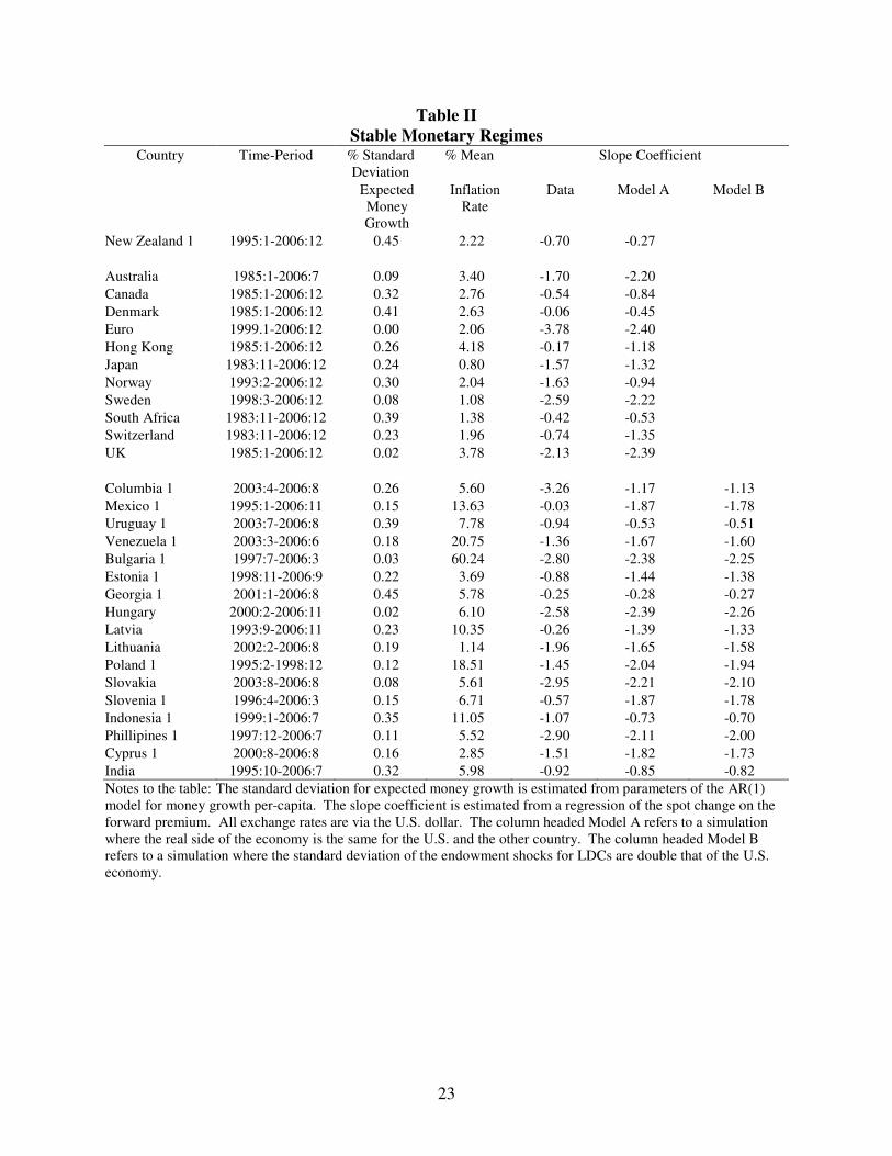
In Table II we present the time period, the standard deviation of the expected monetary growth

per month, the average annual inflation rate and the slope coefficient estimated using actual and

14

simulated data under the stable monetary regime. The slope coefficient estimated using

simulated data is in the column headed Model A for the baseline parameterization and in the

column headed Model B for the simulation where we set the standard deviation of shocks to

endowment growth in LDCs to double that we use for the U.S. In Table III we present the same

statistics for countries that experienced an unstable monetary regime for some time period. If

countries appear (in the first column) in both tables we attach 1 to the country name in the stable

regime and 2 to the country name in the unstable regime. Thirteen out forty-one countries have

both types of regime.

In stable monetary regimes the estimated slope coefficients are typically negative for

developed countries. The model also produces a negative slope coefficient for all developed

countries except New Zealand. The annual growth rates in money per-capita in New Zealand

were very erratic in the first half of the sample, i.e. 1985-94. For the period 1995:1-2006:12

(labelled New Zealand 1 in Table II) the estimated slope coefficient are negative in the data and

the model.

We find that during periods where the monetary regime is stable, when the standard

deviation of expected money growth is low, the estimated slope coefficients in the data and in

the model are negative for less developed countries (in all 17 cases). By contrast, we find that

during periods where the monetary regime is relatively unstable, when the standard deviation of

expected money growth is high, the estimated slope coefficients in the data and in the model are

positive for less developed countries (in all 24 cases).

The results presented in Tables II and III are graphed in Figure I. The South-West

quadrant depicts the case where the slope is negative in the model (read along the vertical axis)

and in the data. The North-East quadrant depicts the case where the slope is positive in the

15

model and in the data. The simple correlation coefficient between the slope coefficient

simulated in the model and estimated in the data is 0.84. All points, with the exception of that

for New Zealand 2, lie in these quadrants and close to the 450 line. For the period the 1985:1-

1994:12 the model produces a positive slope coefficient for New Zealand (labelled New Zealand

2 in Table III) as the standard deviation of expected money growth is much larger than that

estimated for any of the other developed countries (over). However, in the data, the slope

coefficient is estimated to be negative.

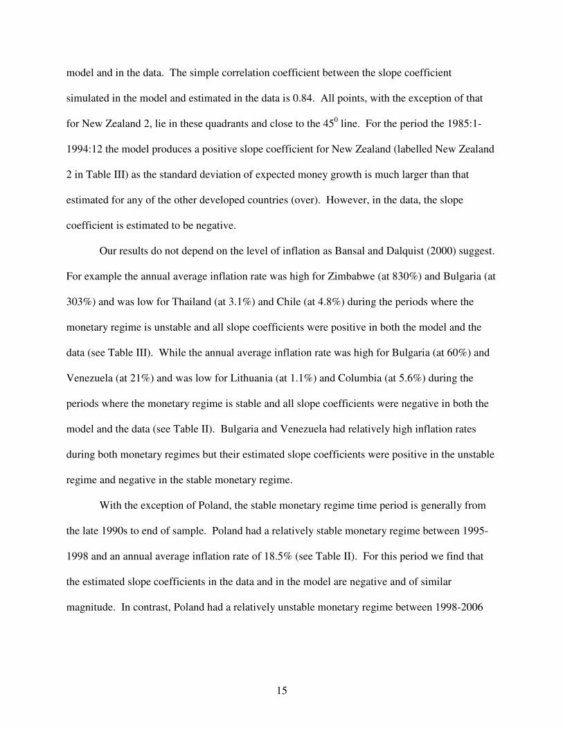
Our results do not depend on the level of inflation as Bansal and Dalquist (2000) suggest.

For example the annual average inflation rate was high for Zimbabwe (at 830%) and Bulgaria (at

303%) and was low for Thailand (at 3.1%) and Chile (at 4.8%) during the periods where the

monetary regime is unstable and all slope coefficients were positive in both the model and the

data (see Table III). While the annual average inflation rate was high for Bulgaria (at 60%) and

Venezuela (at 21%) and was low for Lithuania (at 1.1%) and Columbia (at 5.6%) during the

periods where the monetary regime is stable and all slope coefficients were negative in both the

model and the data (see Table II). Bulgaria and Venezuela had relatively high inflation rates

during both monetary regimes but their estimated slope coefficients were positive in the unstable

regime and negative in the stable monetary regime.

With the exception of Poland, the stable monetary regime time period is generally from

the late 1990s to end of sample. Poland had a relatively stable monetary regime between 1995-

1998 and an annual average inflation rate of 18.5% (see Table II). For this period we find that

the estimated slope coefficients in the data and in the model are negative and of similar

magnitude. In contrast, Poland had a relatively unstable monetary regime between 1998-2006

16

and an annual average inflation rate of 4.5%. For this period we find that the estimated slope

coefficients in the data and in the model are positive and of similar magnitude (see Table III).

4. Conclusion

This paper has proposed a modelling strategy that makes substantial progress towards

explaining why the forward bias puzzle only arises between some pairs of countries and not for

others. A model that combines Campbell and Cochrane (1999) habit persistence defined over

individual goods in a monetary framework identifies two different forces at work. Where

monetary policy is stable, interest rates are primarily determined by real behaviour. In those

circumstances, the importance of the precautionary savings motive ensures that the forward bias

typically arises. This is why uncovered interest parity is not usually observed between

developed countries. In contrast, in countries where monetary instability dominates, something

closer to interest parity is observed because nominal bond holders have to be compensated for

the nominal volatility.

Monetary instability is defined quite precisely here: it is the conditional variance on

money growth. We calibrated this model to 12 developed and 29 emerging economies. We are

successfully able to explain when UIP holds and does not hold without referring explicitly to the

income, inflation rate nor level of development of the countries concerned. As far as we are

aware, we are the first to develop a theoretical model which achieves this.

Obviously, this model is highly stylised. We are assuming complete markets with perfect

international risk sharing. This is particularly difficult when dealing with some of the very

17

underdeveloped economies that we examine here. The evidence of Figure 1 is all the more

compelling because of this.

18

References

Abel, Andrew, (1990), Asset prices under habit formation and catching up with the Joneses,

American Economic Review, Papers and Proceedings 80, 38-42.

Alexius, Annika, (2001), Uncovered interest parity revisited, Review of International Economics

9, 505-517.

Alvarez, Fernando, Andrew Atkeson and Patrick J. Kehoe, (2006), Time-varying risk, interest

rates, and exchange rates in general equilibrium, Federal Reserve Bank of Minneapolis, Staff

Report: 371, available at http://www.minneapolisfed.org/research/SR/SR371.pdf

Bachetta, Philippe and Eric Van Wincoop, (2008), Infrequent portfolio decisions: a solution to

the forward discount puzzle, Mimeo. Available at

http://www.hec.unil.ch/pbacchetta/PDF/forexnew47.pdf

Bansal, Ravi, and Magnus Dahlquist, (2000), The forward premium puzzle: different tales from

developed and emerging economies, Journal of International Economics 51, 115-144.

Bansal, Ravi and Amir Yaron, (2004), Risks for the long run: a potential resolution of asset

pricing puzzles, Journal of Finance 59, 1481-1509.

Bansal, Ravi and Ivan Shaliastovich, (2007), Risk and return in bond, currency and equity

markets, Mimeo. Available at http://faculty.fuqua.duke.edu/~rb7/bio/Bansal_Ivan_June_07.pdf

Burnside, Craig, Martin S. Eichenbaum, and Sergio Rebelo, (2007), Understanding the forward

premium puzzle: a microstructure approach, NBER Working Paper 13278.

Campbell, JohnY. and John H. Cochrane, (1999), By force of habit: a consumption-based

explanation of aggregate stock market behavior, Journal of Political Economy 107, 205-251.

Carlson, John A. and Carol, L. Osler, (2005), Short-run exchange-rate dynamics: theory and

evidence, Mimeo.

19

Chari, V.V., Patrick J. Kehoe, and Ellen R. McGrattan, (2002), Can sticky price models generate

volatile and persistent real exchange rates?, Review of Economics Studies 69, 533-563.

Chinn, Menzie and Guy Meredith, (2004), Monetary policy and long-horizon uncovered interest

parity, IMF Staff Papers 51,409-430.

Chinn, Menzie, (2006), The (partial) rehabilitation of interest rate parity in the floating rate era:

longer horizons, alternative expectations, and emerging markets, Journal of International Money

and Finance 25, 7-21.

Domowitz, Ian and Craig S. Hakkio, (1985) Conditional Variance And The Risk Premium

In The Foreign Exchange Market, Journal of International Economics, 19, 47-66.

Duesenberry, J. S., (1949), Income, saving and the theory of consumer behavior, Cambridge,

Mass.: Harvard University Press.

Eichenbaum, Martin S., (2008), Can peso problems explain carry trade returns?, Paper presented

at Conference on International Macro-Finance, International Monetary Fund. Available at

http://www.ssc.wisc.edu/~cengel/IntWkshp/Eichenbaum.pdf

Engel, Charles, (1996), The forward discount anomaly and the risk premium: a survey of recent

evidence, Journal of Empirical Finance 3, 123-191.

Fama, Eugene F., (1994), Forward and spot exchange rates, Journal of Monetary Economics 14,

319-338.

Fisher, Eric O’N., (2006), The forward premium in a model with heterogeneous prior beliefs,

Journal of International Money and Finance 25, 48-70.

Flood , Robert P., and Andrew K. Rose, (2002), Uncovered interest parity in crisis, IMF Staff

Papers 49, 252-266.

20

Frankel, Jeffrey and Jumana Poonawala, (2009), The forward market in emerging currencies:

less biased than in major currencies, Journal of International Money and Finance, Article in

Press.

Gourinchas, Pierre-Olivier and Aaron Tornell, (2004), Exchange rate puzzles and distorted

beliefs, Journal of International Economics 64, 303-333.

Ito, Hiro and Menzie D. Chinn, (2007), Price-based measurement of financial globalization: a

cross-country study of interest rate parity, Pacific Economic Review 12, 419–444.

Lucas, Robert E., (1982), Interest rates and currency prices in a two-country world, Journal of

Monetary Economics 10, 335-360.

Moore, Michael J. and Maurice J. Roche, (2002), Less of a puzzle: a new look at the forward

forex market, Journal of International Economics 58, 387-411.

Moore, Michael J. and Maurice J. Roche, (2005), A neo-classical explanation of nominal

exchange rate volatility, in Exchange Rate Economics: Where do we stand? edited by Paul de

Grauwe, MIT Press.

Moore, Michael J. and Maurice J. Roche, (2007), Solving exchange rate puzzles with neither

sticky prices nor trade costs, Mimeo. Available at http://www.qub-efrg.com/faculty-

directory/6/michael-moore/

Moore, Michael J. and Maurice J. Roche, (2008), Volatile and persistent real exchange rates with

or without sticky prices, Journal of Monetary Economics 55, 423-433.

Ravn, Morten, Stephanie Schmitt-Grohe and Martin Uribe, (2006), Deep habits, Review of

Economic Studies 73, 195-218.

Ravn, Morten, Schmitt-Grohe, Stephanie and Martin Uribe, (2007). Pricing of habits and the law

of one price. American Economic Review 73, 195-218

21

Sarno, Lucio, (2005), Towards a solution to the puzzles in exchange rate economics: where do

we stand?, Canadian Journal of Economics 38, 673-708.

Verdelhan, Adrien, (2010), A habit-based explanation of the exchange rate risk premium,

Journal of Finance 65, 123-145.

22

Table I

Baseline parameterization

Endowment growth Money growth

Unconditional mean 0.1575% 0.48%

AR(1) coefficient 0.00 0.18

Standard deviation of shock 0.433% 0.55%

Curvature of the utility function γ 2.000

AR1 coefficient of log surplus consumption φ 0.994

Parameter in steady state surplus consumption δ -0.005 Notes to the table: The endowment growth parameters are taken from Campbell and Cochrane (1999) but

transformed to monthly frequency. The money growth parameters are estimated from an AR(1) model for money

growth per-capita using U.S. data over the period 1983:11 to 2006:12. The curvature of the utility function is taken

from Campbell and Cochrane (1999). Following Campbell and Cochrane (1999) the AR1 coefficient of log surplus

consumption is estimated using monthly price-dividend ratio for the U.S. over the period 1983:11 to 2006:12.

23

Table II

Stable Monetary Regimes Country Time-Period % Standard

Deviation

% Mean Slope Coefficient

Expected

Money

Growth

Inflation

Rate

Data Model A Model B

New Zealand 1 1995:1-2006:12 0.45 2.22 -0.70 -0.27

Australia 1985:1-2006:7 0.09 3.40 -1.70 -2.20

Canada 1985:1-2006:12 0.32 2.76 -0.54 -0.84

Denmark 1985:1-2006:12 0.41 2.63 -0.06 -0.45

Euro 1999.1-2006:12 0.00 2.06 -3.78 -2.40

Hong Kong 1985:1-2006:12 0.26 4.18 -0.17 -1.18

Japan 1983:11-2006:12 0.24 0.80 -1.57 -1.32

Norway 1993:2-2006:12 0.30 2.04 -1.63 -0.94

Sweden 1998:3-2006:12 0.08 1.08 -2.59 -2.22

South Africa 1983:11-2006:12 0.39 1.38 -0.42 -0.53

Switzerland 1983:11-2006:12 0.23 1.96 -0.74 -1.35

UK 1985:1-2006:12 0.02 3.78 -2.13 -2.39

Columbia 1 2003:4-2006:8 0.26 5.60 -3.26 -1.17 -1.13

Mexico 1 1995:1-2006:11 0.15 13.63 -0.03 -1.87 -1.78

Uruguay 1 2003:7-2006:8 0.39 7.78 -0.94 -0.53 -0.51

Venezuela 1 2003:3-2006:6 0.18 20.75 -1.36 -1.67 -1.60

Bulgaria 1 1997:7-2006:3 0.03 60.24 -2.80 -2.38 -2.25

Estonia 1 1998:11-2006:9 0.22 3.69 -0.88 -1.44 -1.38

Georgia 1 2001:1-2006:8 0.45 5.78 -0.25 -0.28 -0.27

Hungary 2000:2-2006:11 0.02 6.10 -2.58 -2.39 -2.26

Latvia 1993:9-2006:11 0.23 10.35 -0.26 -1.39 -1.33

Lithuania 2002:2-2006:8 0.19 1.14 -1.96 -1.65 -1.58

Poland 1 1995:2-1998:12 0.12 18.51 -1.45 -2.04 -1.94

Slovakia 2003:8-2006:8 0.08 5.61 -2.95 -2.21 -2.10

Slovenia 1 1996:4-2006:3 0.15 6.71 -0.57 -1.87 -1.78

Indonesia 1 1999:1-2006:7 0.35 11.05 -1.07 -0.73 -0.70

Phillipines 1 1997:12-2006:7 0.11 5.52 -2.90 -2.11 -2.00

Cyprus 1 2000:8-2006:8 0.16 2.85 -1.51 -1.82 -1.73

India 1995:10-2006:7 0.32 5.98 -0.92 -0.85 -0.82

Notes to the table: The standard deviation for expected money growth is estimated from parameters of the AR(1)

model for money growth per-capita. The slope coefficient is estimated from a regression of the spot change on the

forward premium. All exchange rates are via the U.S. dollar. The column headed Model A refers to a simulation

where the real side of the economy is the same for the U.S. and the other country. The column headed Model B

refers to a simulation where the standard deviation of the endowment shocks for LDCs are double that of the U.S.

economy.

24

Table III

Unstable Monetary Regimes Country Time-Period % Standard

Deviation

% Mean Slope Coefficient

Expected

Money

Growth

Inflation

Rate

Data Model A Model B

New Zealand 2 1985:1-2006:12 0.81 4.39 -1.08 0.51

Argentina 2002:02-2006:08 0.87 13.57 1.17 0.52 0.52

Brazil 1980:1-2006:7 7.15 514.83 0.07 0.99 0.99

Bolivia 1995:1-2006:5 0.64 5.19 0.12 0.22 0.22

Chile 1994:1-2006:8 0.82 4.82 0.81 0.47 0.47

Columbia 2 1995:8-2003:3 0.60 13.37 0.01 0.13 0.13

Mexico 2 1986:10-1994:12 1.54 46.31 0.52 0.83 0.83

Uruguay 2 1993:12-2003:06 0.72 20.22 0.69 0.35 0.35

Venezuela 2 1996:1-2003:2 1.01 37.49 1.46 0.63 0.63

Bulgaria 2 1993:12-1997:6 5.76 302.94 1.62 0.99 0.99

Estonia 2 1993:9-1998:10 1.14 25.49 0.23 0.71 0.71

Georgia 2 1995:12-2000:12 1.46 15.82 1.22 0.81 0.81

Poland 2 1999:1-2005:12 0.74 4.46 0.58 0.37 0.37

Romania 1995:8-2006:11 0.94 41.25 0.40 0.58 0.58

Russia 1995:6-2006:8 0.58 36.10 0.45 0.09 0.10

Slovenia 2 1991:12-1996:3 0.68 21.70 0.25 0.29 0.29

Indonesia 2 1994:1-1998:12 0.65 18.02 0.79 0.23 0.23

Phillipines 2 1992:1-1997:11 0.59 7.82 0.40 0.10 0.10

South Korea 1980:1-2006:05 1.14 6.12 0.45 0.71 0.70

Thailand 1997:8:2006:8 1.20 3.11 0.45 0.73 0.73

Cyprus 2 1996:1-2000:7 3.00 2.84 0.12 0.95 0.95

Israel 1984:6-2006:6 1.16 38.18 0.38 0.72 0.71

Nigeria 2001:12-2006:06 2.18 14.59 0.63 0.91 0.91

Turkey 1986:4-2006:7 2.03 58.02 0.64 0.90 0.90

Zimbabwe 2004:1-2006:10 1.45 830.33 0.40 0.81 0.81

Notes to the table: The standard deviation for expected money growth is estimated from parameters of the AR(1)

model for money growth per-capita. The slope coefficient is estimated from a regression of the spot change on the

forward premium. All exchange rates are via the U.S. dollar. The column headed Model A refers to a simulation

where the real side of the economy is the same for the U.S. and the other country. The column headed Model B

refers to a simulation where the standard deviation of the endowment shocks for LDCs are double that of the U.S.

economy.

25

Figure 1. Comparison of Theoretical and Estimated Fama regression slopes.

Notes to the figure: The slope is obtained from a linear regression of the expected spot return on the forward

discount or nominal interest rate differential. The estimated slope using actual data is plotted along the horizontal

axis. The estimated slope from the theoretical model is plotted along the vertical axis.

26

Appendix 1: Calculating unconditional second moments

In this appendix we derive the conditional moments in the Fama (1994) regression (11). Using

(19) the unconditional variance of the expected spot change is:

( )( ) ( )1 2

2 2 2 22 2 2 21 1 2 2

1 2 2

1 2

(1 )1 1

u ut t t x x

Var E s s π π

π π

ρ σ ρ σφ γ σ σ

ρ ρ+

− = + + − +

− − (22)

The covariance between expected forward profits (17) and the expected spot return (19) is:

( ) ( )( )( ) ( ) ( )( )

( ) ( )( )

1

2

2

1 1 1

2

2

, 1 1

1 1

t t t t t t x

x

Cov f E s E s s γ φ γ φ θ σ

γ φ γ φ θ σ

+ + − − = − − − +

− − − + (23)

Given our baseline parameter values discussed in Section 3 the covariance (23) is negative,

which is one of Fama’s necessary conditions for a negative slope. Using (18) the unconditional

variance of the forward discount is:

( ) ( )1 1 2 2

1 2

1 2

2 2 2 2

2 2 2 2

1 22 21 1

u ut t x x

Var f s π π

π π

ρ σ ρ σθ σ θ σ

ρ ρ− = + + +

− − (24)

27

Appendix 2: Data

Developed countries

For developed countries the exchange rates are the end of period spot and one-month forward

exchange rates (BBI) and are obtained from Datastream Advance. For Japan, Canada and

Switzerland, the money supply is the monetary base and is available from Reuters Ecowin.

For the remaining developed countries the money supply is M1 from the OECD main economic

indicators and is available from Reuters Ecowin. The sample periods are determined by data

availability. The sample periods are Australia (1985:1-2006:7), Canada (1985:1-2006:12),

Denmark (1985:1-2006:8), the Euro(1999:1-2006:12), Hong Kong (1985:3-2006:12), Japan

(1983:11-2006:12), New Zealand (1985:1-2006:12), Norway (1993:2-2006:12), South Africa

(1983:11-2006:12), Sweden (1998:3-2006:12), (Switzerland) 1983:11-2006:12) and UK

(1986:10-2006:12).

Developing countries

The data on eurodollar and interbank interest rates, spot and forward exchange rates (BBI) are

available from Datastream Advance. The data on M1 (from OECD main economic indicators)

and the money base (from individual country statistics offices) is available from Reuters Ecowin.

The data on deposit, money market and Treasury bill interest rates, some exchange rates,

population and the money supply are from the IMF International Financial Statistics database

which is available from Reuters Ecowin. The sample periods are determined by data availability

and whether the exchange rate was a market driven rate. The sample periods are Argentina

(2002:2-2006:8), Brazil (1980:1-2006:7), Bolivia (1995:5-2006:5), Chile (1994:1-2006:8),

Columbia (1995:8-2006:7), Mexico (1986:10-2006:11), Uruguay (1993:12-2006:8), Venezuela

28

(1996:1-2006:6), Bulgaria(1993:12-2006:3), Estonia (1993:9-2006:9), Georgia (1995:12-

2006:8), Hungary (2000:2-2006:11), Latvia (1993:9-2006:11), Lithuania (2002:2-2006:8),

Poland (1995:2-2005:12), Romania (1995:8-2006:11), Russia (1995:6-2006:8), Slovakia

(2003:8-2006:8), Slovenia (1991:12-2006:3), Indonesia (1994:1-2006:7), South Korea (1980:1-

2006:5), Phillipines (1992:1-2006:7), Thailand (1997:8-2006:8), Cyprus (1996:1-2006:11),

India (1995:10-2006:7), Israel (1984:6-2006:6), Nigeria (2001:12-2006:6), Turkey (1986:4-

2006:7), and Zimbabwe (2004:1-2006:10).