For Peer Review - USC Marshall · For Peer Review Demand Learning and A greement Delay in...

For Peer Review

Demand Learning and Agreement Delay in Technology

Adoption

Journal: Manufacturing and Service Operations Management

Manuscript ID MSOM-16-416

Manuscript Type: Innovative Operations

Keywords: Technology Management and Process Design, Game Theory, Pricing and

Revenue Management

ScholarOne, 375 Greenbrier Drive, Charlottesville, VA, 22901

Manufacturing & Service Operations Management

For Peer Review

Demand Learning and Agreement Delay

in Technology Adoption

Abstract

Negotiations associated with technology adoption can take months or years and agreements

are often made close to deadlines. Existing theories attribute agreement delay and the dead-

line effect in bilateral negotiations to either asymmetric information or behavioral constraints.

However, high-technology industries are often characterized by deep cooperation, effective

communications, rational decisions, and uncertain demand for new technologies. We study

the drivers and consequences of agreement delay in this context with a bilateral, dynamic

bargaining model featuring uncertain demand facing the seller, information symmetry, and

a deadline. We discover that incentives to learn about the seller’s demand drive delay of

agreements. With better information, the seller can possibly sell the manufacturing capacity

to higher-value buyers; the buyer can also benefit from learning because the seller must make

concessions if they find the demand to be weak. Thus, delay can be efficient and benefit both

negotiators. However, we also show a sufficient condition under which delay hurts the buyer.

Although extending the deadline can improve the joint payoff, close deadlines are preferred

by the buyer when the buyer has a sufficiently low bargaining power or when the seller with a

strong bargaining power is very likely to have excessive capacities.

[Keywords: technology adoption; bargaining; demand learning; delayed agreement; revenue

management]

1

Page 1 of 37



123456789101112131415161718192021222324252627282930313233343536373839404142434445464748495051525354555657585960

For Peer Review

1 Introduction

Drawn-out negotiations and delayed agreements are common when new manufacturing or com-

ponent technologies are adopted along supply chains. Existing theories generally attribute this

delay and the so-called “deadline effect” (i.e., agreements are prone to be achieved close to the

deadline) to asymmetric information (e.g., Cramton 1984), random delay of price offers (Ma and

Manove 1993), or history-dependent preferences (Fershtman and Seidmann 1993 and Li 2007).

Without these conditions, agreements should be immediately reached in bilateral negotiations

(e.g., Robinstein 1982 and Muthoo 1999). However, high-technology industries such as the mi-

croprocessor market are often characterized by deep cooperation, efficient communications, and

professional decisions. Hence, we are still uncertain as to why firms in such industries often can-

not reach agreements until the last minute.

A recent example involves Apple, Inc. and Taiwan Semiconductor Manufacturing Company

(TSMC) in the microprocessor market. According to The Wall Street Journal, since July of 2014,

Apple and TSMC have collaborated on designing and testing the 14/16-nanometer A9 processor

that would power 2015 iPhones and iPads (Luk 2014). Hundreds of TSMC engineers were sent to

Apple headquarters to work on the project. Apple finally decided to award nearly one-third of the

A9 processor orders to TSMC around April of 2015, after vacillating between GlobalFoundries and

TSMC for more than half a year (Hughes 2015). It was reported, however, that the price was still

unsettled for this deal even in August of 2015 when TSMC already had its 14/16-nanometer Fin-

FET Process capacity ready and the new iPhone was due to be launched soon (Lien and Shen 2015).

According to an August 2015 article in DigiTimes.com, Apple requested price cuts from both its

A9 processor suppliers, Samsung Electronics and TSMC. TSMC, however, was not inclined to

drop prices given that its 16-nanometer FinFET process had been adopted by downstream buyers

such as Broadcom, Freescale Semiconductor, Nvidia, and MediaTek, among others, who could be

potential users of TSMC’s capacity.

Although infrequent, such delayed agreements are not unusual in high-technology industries.

In another example, although Nvidia officially named Samsung to be its manufacturing partner

in early 2015 and aimed to adopt Samsung’s 14nm low-power plus fabrication process, the deal

was still not finalized in June 2015, due to prolonged negotiations (Shilov 2015). According to an

2

Page 2 of 37



123456789101112131415161718192021222324252627282930313233343536373839404142434445464748495051525354555657585960

For Peer Review

article from kitguru.net,

“Nvidia’s chip designers are working on chips to be made by Samsung, whereas other

people are negotiating over pricing. If talks take too much time, then the start of vol-

ume production may be delayed, but since Nvidia will need Samsung’s production

services only in 2016, it still has weeks or even months to negotiate a deal.”

More recently, Apple decided to switch from LCD (liquid crystal display) to OLED (organic light-

emitting diode) panels for its 2017 iPhone and entered into negotiations with Samsung in Novem-

ber 2015 for the supply of the new panels (Singh 2015). Although Samsung had already signed a

previous contract to supply OLED panels for the Apple watch, the iPhone contract was signed in

April, 2016, after negotiations that lasted for several months (Ungureanu 2016). In fact, according

to our interactions with practitioners, many other examples of delayed price agreement exist in

high-technology industries but have not been covered by news reports.

The aforementioned examples motivate us to think about the following questions. Why do

firms fail to reach an immediate agreement (e.g., within a day or so) when they have symmetric

information and make concessions when rejections to their price offers are anticipated? Does de-

lay benefit or hurt firms in high-technology industries? What is the impact of a deadline? As far as

we are concerned, no clear answers to these questions can be found in the literature. Traditional

strategic bargaining models that build on Robinstein (1982) and assume information symmetry

often predict immediate agreement. The reason is that delay is costly and unnecessary because

the consequences can be rationally expected and avoided by making concessions as long as both

players benefit from the trade. In addition, traditional models normally assume that outside op-

tions are fixed and known; hence, no new information can be collected over time and thus delay

will always hurt both firms.

An important feature of high-technology industries not captured by traditional models is that

demand for new technologies is uncertain and thus the seller’s outside option is unknown to both

the buyer and seller at the outset of negotiations. The demand of a new technology depends on

the number of firms that decide to adopt the technology. Normally, as these adoption decisions

are publicly announced or reported by the media (e.g., Luk 2014 and Ungureanu 2016), both the

buyer and seller learn about the demand over time. As a result, both parties may have incentives

3

Page 3 of 37



123456789101112131415161718192021222324252627282930313233343536373839404142434445464748495051525354555657585960

For Peer Review

to delay the agreement. On the one hand, if many new buyers adopt the technology after the start

of the negotiation with the focal buyer, the seller then would like to charge more for production

capacity. On the other hand, the buyer may also benefit from better information regarding the

demand because the seller may have to make concessions if they find that the demand is weak.

Therefore, demand learning is a critical component of negotiation in high-technology industries.

Other important features of high-technology industries, especially the semicondutor industry,

include price negotiations, expensive and inflexible production capacities, and inflexible procure-

ment quantities. Because manufacturing facilities are costly and construction lead times are long,

suppliers often build up their capacities based on demand forecasts and the capacities are inflex-

ible during a selling season. OEM buyers often take advantage of this situation and drive hard

bargains. Lacking full pricing power, suppliers are unable to set the price in a take-it-or-leave-it

fashion and have to engage in negotiations. Normally, the purchase quantity is not a term for

negotiation. This is because final products are often made of a large number of components, it

is difficult for buyers to manipulate the procurement quantity of a particular one. Readers are

referred to Karabuk and Wu (2003) and Zhang et al. (2016) for detailed descriptions of the semi-

conductor industry.

In this research, we focus on a setting wherein an OEM decides to adopt the technology offered

by a supplier for the next generation of product and has determined the production plan of the

final product as well as the purchase quantity of the focal component. (Although buyers in prin-

ciple can allocate their purchase requirements among alternative suppliers, they do so at a very

early stage in the planning process because products offered by different sellers differ in technical

features and influence the design of the buyer’s products. The change of order allocation later

on can thus incur huge costs due to change of production plan and renegotiations.) Therefore,

the buyer’s only task is to negotiate with the supplier for the price before a fixed deadline. Moti-

vated by the microprocessor market, we build a strategic bargaining model that has the following

features: (1) the buyer and seller always have symmetric information; (2) a deadline for the nego-

tiation exists; (3) the seller has a fixed capacity; (4) the market condition is unknown at the outset;

(5) new adopters of the technology appear sequentially and randomly; and (6) the belief about the

market condition is updated over time. Using this model, we learn that the delay of agreement

is driven by incentives to learn, and learning can benefit both the seller and buyer. Contradicting

4

Page 4 of 37



123456789101112131415161718192021222324252627282930313233343536373839404142434445464748495051525354555657585960

For Peer Review

most existing models that show delay is inefficient and that extending the deadline can hurt the

participants, we show that expected payoffs can be improved by extending the deadline given that

delay is costly and that the “deadline effect” exists—that is, agreements are frequently achieved

either at the beginning or near the deadline. Of course, extending the deadline can sometimes

hurt the negotiators, and we show when such situations occur. Particularly, the buyer can suffer

from extending the deadline when his bargaining power is really low or when high demand for

the technology is very unlikely (and the seller is likely to have excessive capacities). In addition,

we find that the tendency of delay increases as more technology adopters appear and the belief

of high demand gets stronger, which offers a partial explanation to the agreement delay between

Apple and TSMC. These results hold even if we allow the value of the technology to depend on

the market condition, or if we extend the model in a number of other ways.

2 Related Literature

This paper is related to three streams of research in the literature: sales management in new prod-

uct or technology diffusion and adoption; bargaining with delay of agreements; and bargaining

in supply chains. As far as we know, our paper is the first to explicitly model the process of B2B

bargaining during new technology diffusion and adoption.

The literature of sales management in new product or technology diffusion and adoption is

primarily based on the diffusion model proposed by Bass (1969). Robinson and Lakhani (1975)

conducted the first study of a dynamic pricing problem of a seller who faces a price-dependent

demand process, which is represented by an extended Bass model. Krishnan et al. (1999) then

proposed the generalized Bass model and developed an optimal pricing path that is consistent

with empirical data. These two papers assume that the seller has the absolute pricing power and

thus they do not consider bargaining. More recently, Ho et al. (2002), Kumar and Swaminathan

(2003), and Shen et al. (2011) studied the management of demand and sales dynamics in new

product diffusion under supply constraint. In their models, a seller can turn down the request of

a customer who then either waits or exits the market and thus delay of sales is possible. While

Ho et al. (2002) showed that it is never optimal to refuse to satisfy any customers when a firm

has inventory, Kumar and Swaminathan (2003) and Shen et al. (2011) argued that production

5

Page 5 of 37



123456789101112131415161718192021222324252627282930313233343536373839404142434445464748495051525354555657585960

For Peer Review

constraints may in fact lead a firm to reject customer orders even when the firm has the inventory.

However, this unintuitive but optimal behavior of denying customers disappears when the firm

can dynamically set prices. Different from all of these studies, our paper is based on a strategic

bargaining model and we focus on the time of agreement between a seller and a major buyer

while they jointly learn about the demand of the new technology. Although learning models (e.g.,

Jensen 1982 and McCardle 1985) have been used in the literature of technology adoption to predict

delay of adoption, they mostly focus on single-firm problems. To the best of our knowledge, our

work is the first to consider bilateral negotiations in technology adoption. Our model suggests

that even though agreement delay allows learning and thus can increase supply chain efficiency,

delay may hurt one of the negotiating parties under certain circumstances.

Delay in reaching agreements has been frequently observed in practice and studied in the lit-

erature. So far, four causes of delay have been discussed in the literature: information asymmetry,

random delay of price offers, history-dependent preferences, and multi-person sequence game.

Cramton (1984) was among the earliest to study the phenomenon that trade often occurs after a

costly delay and attributed the delay to the need for participants to learn each other’s valuation

under incomplete information. Later, Admati and Perry (1987) and Cramton (1992) proposed that

bargainers can signal the strength of their bargaining positions by delaying. Fuchs and Skrzypacz

(2010) studied a model that combines information asymmetry and the arrival of new buyers. They

assumed that the seller has an indivisible good to sell, the seller does not know the value of the

good for the focal buyer, and the negotiation will be terminated when a new buyer randomly ar-

rives. Because the type of buyer is unknown, the seller gradually lowers the asking price and thus

the agreement is delayed until a buyer accepts the price. In this model, the agreement delay is

mainly driven by information asymmetry, and there is no learning about an outside option, which

is the main feature of our model. In the latest paper in this stream, Feng et al. (2015) predicted

a delay in price-quantity contract settlement in supply chains wherein the demand information

is known only to the buyer. In all of the aforementioned papers, delay is driven by information

asymmetry and an infinite horizon is assumed. Roth et al. (1988) considered bargaining with

deadlines and documented some experimental evidence of last-minute agreements. Based on this

observation, Ma and Manove (1993) proposed a continuous-time, alternating-offer model with a

deadline and symmetric information. They assumed that players can decide when to make an

6

Page 6 of 37



123456789101112131415161718192021222324252627282930313233343536373839404142434445464748495051525354555657585960

For Peer Review

offer or counteroffer but only after an exogenous, random delay due to information transmission

and processing. Their model predicts that players adopt strategic delay early in the game and

reach an agreement late in the game if at all. Because the player who makes an offer closer to

the deadline is less likely to be rejected, the delay in the model is driven by the desire to obtain

a stronger bargaining power. However, long and random communication lead time is not an ap-

propriate assumption in high-technology industries. Recently, Damiano et al. (2012) studied a

concession game wherein two players jointly decide between two alternatives and the value of

each option is different for the two players and is privately known. They showed that delay of

agreement can hurt or benefit the players and there exists an optimal deadline. The cause of delay

in their model is again information asymmetry. Under the assumption of symmetric informa-

tion, the models proposed by Fershtman and Seidmann (1993) and Li (2007) both predict delay of

agreement; however, their models deviate from the assumption of rational behavior and rely on

history-dependent commitment or preferences. Cai (2000) studied delay of agreement in multilat-

eral bargaining with symmetric information. In the model, if weak players who reach agreements

earlier can be forced to accept much smaller shares than tough players who reach agreements later,

then delay can arise; in other words, the sequence matters. Assuming symmetric information, we

contribute to this literature by offering a new explanatory factor of delay: learning about the ex-

istence of other buyers. Furthermore, while nearly all of the previous studies argue that delay is

inefficient, we offer a counter argument that delay can benefit both parties.

The literature on multilateral bargaining in B2B markets or supply chains has emerged in re-

cent years and this stream of research normally focuses on how profit is allocated among supply

chain members. Depending on the game structure that is used, two streams of research mainly

exist in this literature. One stream assumes that the multilateral bargaining happens sequentially

and considers the impact of the bargaining sequence and coalitions. In an assembly-chain set-

ting, Nagarajan and Bassok (2008) considered suppliers who form multilateral bargaining coali-

tions and compete for a position in the bargaining sequence. Different from sequential models in

which bargaining power is manifested in the position in the sequence, simultaneous multilateral-

negotiation models focus on the static equilibrium in which the profit allocation is determined

by a negotiator’s contribution to the entire system. Guo and Iyer (2013) compared simultane-

ous and sequential multilateral bargaining games in a channel system with one manufacturer

7

Page 7 of 37



123456789101112131415161718192021222324252627282930313233343536373839404142434445464748495051525354555657585960

For Peer Review

and two competing retailers. They show that the manufacturer’s choice of timing of bargain-

ing—i.e., simultaneous versus sequential bargaining—should depend on the dispersion in retail

prices. Dukes et al. (2006) and Lovejoy (2010) used simultaneous bargaining models to study

the impact of a channel or chain structure. In a retail setting, Aydin and Heese (2015) studied

an assortment problem of a retailer who engages in simultaneous bilateral negotiations with all

manufacturers for a given assortment. Our model falls into the realm of sequential bargaining,

but we supplement the literature by studying the situation wherein the number of participants is

uncertain. In addition, we focus on the demand-learning process and efficient capacity allocation

during technology adoption.

3 The Base Model

Supplier A sells a new component or process technology with a fixed capacity to multiple OEM

(original equipment manufacturer) buyers over multiple periods. Due to heterogeneity in de-

velopment cycles, the buyers may decide to adopt the new technology at different times. In the

semiconductor industry, buyer adoption decisions are often called design-wins of the seller, and

such decisions indicate future demand. Without loss of generality, we assume that a major buyer,

B, is the first adopter and starts a negotiation with sellerA in period 1. WhileA and B are negoti-

ating, design-wins may be achieved with other buyers. We define each period to be short enough

so that at most one design-win can be achieved at the beginning of a period. Because the number

of buyers is finite, the arrival process of design-wins will end. When potential adopters exist, a

new design-win will be achieved in a period (t > 1) with probability α ∈ (0, 1).

Motivated by the Apple-TSMC as well as the Nvidia-Samsung example, we focus on a setting

wherein B has decided to adopt the technology for the next generation of product and the overall

production plan as well as the launch date of the new product has been determined. Hence,

there is a deadline for B to reach an agreement. However, the time of agreement will not affect

the production plan or the launch date of the final product. We consider that B has to reach an

agreement by period T ≥ 1; otherwise, B has to give up the technology and receive a fixed payoff

that is normalized to zero. Note that seller A may continue the selling after period T. Because

the final product is made of different components, it is difficult for B to change the procurement

8

Page 8 of 37



123456789101112131415161718192021222324252627282930313233343536373839404142434445464748495051525354555657585960

For Peer Review

quantity of a particular one. We thus consider that B demands Q > 0 units of capacity from A

and partial fulfillment is not accepted.

We focus on the negotiation between A and B, which proceeds as follows. In each period,

one party, either A or B, is randomly selected to propose a price. If the other party accepts the

price, an agreement is reached. Otherwise, both parties wait until the next period and the process

repeats. Such a random-proposer bargaining game is common in the economics literature. Similar

settings can be found in Binmore (1987), Fershtman and Seidmann (1993), and Muthoo (1999). We

assume that buyer B’s relative power of bargaining is measured by β ∈ (0, 1) such that B proposes

the price in any period with probability β. This is because the proposer can set the price to the

reservation price of the other party when an agreement is possible and thus seize a larger share

of the surplus. To be consistent with the classic strategic bargaining models (e.g., Rubinstein 1982

and Muthoo 1999), we do not allow the players to quit the negotiation in the base model unless the

bargaining breaks down. We define break-downs later in this section and the option of quitting

will be discussed in Section 6.4.

The total number of adopters, N, including buyer B, is unknown at the beginning. Two possi-

ble market conditions exist: an average market, wherein N = NL ≥ 1, or a good market, wherein

N = NH > NL. Therefore, both A and B can learn about the market condition by counting the

arrival of design-wins. Once the critical number, NL + 1, is observed, both parties can be sure that

the market is good. It is a common prior belief that Pr {N = NH} = γ ∈ (0, 1). Let Nt denote the

total number of adopters that have appeared by period t and we have N1 = 1. According to the

Bayes’ theorem, we know that

Pr {N = NH |Nt < NL, t > 0} = γ;

Pr {N = NH |Nt > NL, t > 0} = 1;

Pr {N = NH |Nt′−1 < NL, Nt′ = NL, Nt′+t = NL, t ≥ 0} = γ(1− α)t

1− γ + γ(1− α)t .

Hence, the belief about the market condition in period t depends on the history, {Nk}tk=1. Let

θt = Pr{

N = NH | {Nk}tk=1

}be the belief in period t and π be seller A’s opportunity cost per unit

of the capacity demanded by buyer B. In other words, A can obtain an expected profit of Qπ if

the capacity is not sold to buyer B. For the sake of tractability, we assume that π = 0 in an average

9

Page 9 of 37



123456789101112131415161718192021222324252627282930313233343536373839404142434445464748495051525354555657585960

For Peer Review

market and π = π0 > 0 in a good market. Before N or the market condition is known, the per-unit

opportunity cost in period t is thus πet = θt · π0.

Although a two-point distribution of the market condition is a simplification, it can actually be

mapped to certain realistic situations. For example, in practice, potential adopters can usually be

classified into two types: strategic partners and market followers. Strategic partners will definitely

adopt the technology, and market followers will adopt the technology if the market believes that

the technology is promising. In this case, the firms can be sure that the market condition is good

if one of the market followers decides to adopt the technology. Readers are referred to Section 6.3

for further discussion. In addition, notice that negotiations between the supplier and other buyers

during the process will not influence the negotiation with B as long as π = 0 or Nt ≤ NL. Once the

market condition is known to be good, no more delay is necessary and the supplier has to decide

whether to reach an agreement with B or terminate the negotiation.

For the buyer, it is publicly known that each unit of the capacity has a fixed value of v > 0.

For the seller, we set the marginal production cost to zero because a positive production cost

will not qualitatively change the results. Even if the production cost depends on whether an

agreement is reached, the difference can be capture by the supplier’s opportunity cost. In addition,

bargaining and delaying the agreement are costly for both the seller and buyer because bargaining

consumes labor hours and delaying the agreement may cause delay of other business activities

such as marketing and pricing. It costs the seller cS > 0 and the buyer cB > 0 per period unless an

agreement has been reached or the bargaining breaks down. Both cS and cB are public information.

Finally, the negotiation terminates either when an agreement is achieved or the negotiation

breaks down. The negotiation breaks down either (1) when the deadline is reached, or (2) when

the market condition is known yet an agreement is not achieved. The timing of events in a period

is summarized in Figure 1.

4 Model Analysis

This is a non-stationary, strategic bargaining model with symmetric information and two-sided

learning. We know that the result of a bargaining game depends on the bargaining powers, the

value of trade, and the outside options. The bargaining powers (i.e., β and 1− β) and the value

10

Page 10 of 37



123456789101112131415161718192021222324252627282930313233343536373839404142434445464748495051525354555657585960

For Peer Review

Figure 1: The Timing of Events in Period t

of trade (i.e., vQ) are fixed in this game, but the outside options may change as the players learn

about the market. As described in the previous section, the buyer’s outside option is 0 and the

seller’s outside option is πet = θt · π0 per unit of capacity. Clearly, an agreement can be reached in

period t only if v ≥ θt ·π0; however, an agreement may not be reached even if v ≥ θt ·π0. Our goal

in this section is to understand how θt evolves and when an agreement can be reached. Because

the bargaining has a deadline, we will use a backward induction to solve this dynamic game.

First, notice that θt is a function of {Nk}tk=1 and from the firms’ perspective the evolution of

{Nk}tk=1 in turn depends on θt. Hence, define the state in period t as st = {Nt, θt}. We know that

when Nt < NL, the arrival process of design-wins is always on and there is no learning. Hence,

for Nt < NL, the state evolves in the following way:

Nt+1 =

Nt + 1 w.p. α

Nt w.p. 1− α

and θt+1 = θt = γ.

The learning takes place when Nt ≥ NL. Specifically, Nt+1 = Nt + 1 if N = NH and a new adopter

arrives. Once Nt > NL, we can confirm that N = NH; otherwise, we update the belief. Hence, for

Nt ≥ NL, the transition takes the following form:

Nt+1 =

Nt + 1 w.p. αθt

Nt w.p. 1− αθt

and θt+1 =

1 if Nt+1 > NL

(1−α)θt(1−α)θt+1−θt

if Nt+1 = NL

.

11

Page 11 of 37



123456789101112131415161718192021222324252627282930313233343536373839404142434445464748495051525354555657585960

For Peer Review

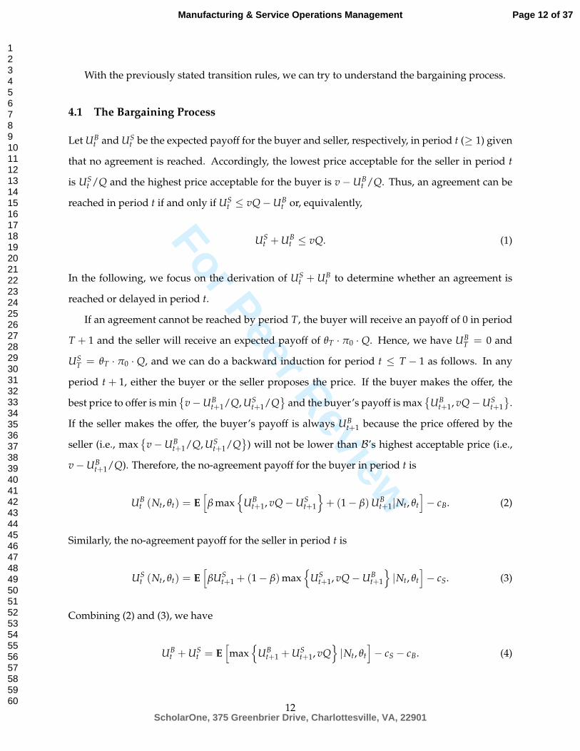
With the previously stated transition rules, we can try to understand the bargaining process.

4.1 The Bargaining Process

Let UBt and US

t be the expected payoff for the buyer and seller, respectively, in period t (≥ 1) given

that no agreement is reached. Accordingly, the lowest price acceptable for the seller in period t

is USt /Q and the highest price acceptable for the buyer is v−UB

t /Q. Thus, an agreement can be

reached in period t if and only if USt ≤ vQ−UB

t or, equivalently,

USt + UB

t ≤ vQ. (1)

In the following, we focus on the derivation of USt + UB

t to determine whether an agreement is

reached or delayed in period t.

If an agreement cannot be reached by period T, the buyer will receive an payoff of 0 in period

T + 1 and the seller will receive an expected payoff of θT · π0 · Q. Hence, we have UBT = 0 and

UST = θT · π0 · Q, and we can do a backward induction for period t ≤ T − 1 as follows. In any

period t + 1, either the buyer or the seller proposes the price. If the buyer makes the offer, the

best price to offer is min{

v−UBt+1/Q, US

t+1/Q}

and the buyer’s payoff is max{

UBt+1, vQ−US

t+1

}.

If the seller makes the offer, the buyer’s payoff is always UBt+1 because the price offered by the

seller (i.e., max{

v−UBt+1/Q, US

t+1/Q}

) will not be lower than B’s highest acceptable price (i.e.,

v−UBt+1/Q). Therefore, the no-agreement payoff for the buyer in period t is

UBt (Nt, θt) = E

[β max

{UB

t+1, vQ−USt+1

}+ (1− β)UB

t+1|Nt, θt

]− cB. (2)

Similarly, the no-agreement payoff for the seller in period t is

USt (Nt, θt) = E

[βUS

t+1 + (1− β)max{

USt+1, vQ−UB

t+1

}|Nt, θt

]− cS. (3)

Combining (2) and (3), we have

UBt + US

t = E[max

{UB

t+1 + USt+1, vQ

}|Nt, θt

]− cS − cB. (4)

12

Page 12 of 37



123456789101112131415161718192021222324252627282930313233343536373839404142434445464748495051525354555657585960

For Peer Review

Using this iteration formula, we can derive the following results. Lemma 1 suggests that if bar-

gaining is too costly for either party or the capacity is of high value to the buyer, an agreement

will be reached immediately. This result is independent of bargaining power β. We then derive a

necessary condition for the delay of agreement by introducing Proposition 1. Note that all of the

technical proofs are presented in the supplementary.

Lemma 1. An agreement can be reached in period t < T if and only if

cS + cB ≥ E[max

{0, UB

t+1 + USt+1 − vQ

}|Nt, θt

]. (5)

Proposition 1. If vQ + cS + cB ≥ π0Q, the agreement is never delayed.

To study possible delays of the agreement, we now assume that π0Q > vQ + cS + cB for the

rest of our analysis. In preparation, define

δt (Nt, θt) =UBt (Nt, θt) + US

t (Nt, θt) + cS + cB − vQ

=E[max

{0, UB

t+1 + USt+1 − vQ

}|Nt, θt

]=E [max {0, δt+1 − cS − cB} |Nt, θt] . (6)

Accordingly, we know that δt (Nt, θt) ≥ 0 and UBt + US

t = vQ− cS − cB + δt for period t ≤ T − 1.

In light of Lemma 1, an agreement can be reached if and only if

δt ≤ cS + cB. (7)

Hence, δt can be viewed as the tendency of delay in period t. Again, it is important to notice that δt

is independent of the bargaining power β.

We now perform a backward induction on UBt +US

t , starting from period T, and the procedures

are illustrated in Table 1. From the table, we can see that the key is to determine the value of δt for

each period t and then we know the dynamics of the bargaining process. However, it is difficult

to determine the values directly. Given that δt can be written iteratively as a function of δt+1, we

will try to derive some structural properties of δt and the bargaining process in the next section.

13

Page 13 of 37



123456789101112131415161718192021222324252627282930313233343536373839404142434445464748495051525354555657585960

For Peer Review

Table 1: Backward Induction on UBt + US

t Given π0Q > vQ + cS + cB

PeriodCase:

Nt < NL

Case:Nt = NL

Case:Nt > NL

T π0γQ π0θTQ π0Q

T − 1 Q ·max {π0γ, v} − cS − cBQ ·max {π0θT−1, v + αθT−1 (π0 − v)}

−cS − cB π0Q

T − 2

For NT−2 < NL − 1 :vQ− cS − cB+ [(π0γ− v) Q− cS − cB]

+

For NT−2 = NL − 1 :vQ− cS − cB + δT−2 (NL − 1, γ)

vQ− cS − cB + δT−2 (NL, θT−2) π0Q

· · · · · · · · · · · ·

t

For Nt < NL − (T − t− 1) :vQ− cS − cB+ [(π0γ− v) Q− cS − cB]

+

For Nt ≥ NL − (T − t− 1) :vQ− cS − cB + δt (Nt, γ)

vQ− cS − cB + δt (NL, θt) π0Q

Note:

δT−1 (NL − 1, γ) = Q ·max {0, π0γ− v}δT−1 (NL, θT−1) = Q ·max {π0θT−1 − v, αθT−1 (π0 − v)}δT−2 (NL − 1, γ) = (1− α)max {0, δT−1 (NL − 1, γ)− cS − cB}

+ α max {0, δT−1 (NL, γ)− cS − cB}δT−2 (NL, θT−2) = θT−2α (π0 − v) Q + (1− θT−2α)max

{δT−1

(NL, (1−α)θT−2

1−αθT−2

)− cS − cB, 0

}x+ = max{0, x}

14

Page 14 of 37



123456789101112131415161718192021222324252627282930313233343536373839404142434445464748495051525354555657585960

For Peer Review

4.2 Delay of the Agreement

Given that π0Q > vQ + cS + cB, we can easily prove that UBt + US

t ≤ π0Q for any t, Nt, and θt,

using (4) and induction. It means that the total no-agreement payoff should be bounded by π0Q,

the total opportunity loss for the seller in a good market. With this observation, we can proceed

to prove the following result.

Proposition 2. δt (Nt, θt) is an increasing function of π0 given any possible t, Nt, and θt.

Note that π0 carries the influence from several factors, including the capacity level, the differ-

ence in demand between the two market conditions, other buyers’ valuation of the component,

and their bargaining powers. It is reasonable to expect that the tendency of delay increases as the

supplier’s opportunity cost increases. This is because higher opportunity cost implies higher ben-

efit the supplier could obtain from learning and thus better allocation of the capacity. On the other

hand, the buyer has an high incentive to learn about the market condition when π0 is high be-

cause if they agree immediately the joint surplus (i.e., vQ−π0θtQ) is small and thus the buyer has

to pay a high price. Thus, from the buyer’s standpoint, the downside of delay is limited but the

upside is high. Although this logic also applies to the next result, the proof is more complicated.

Proposition 3. δt (Nt, θt) is an increasing function of θt given any possible t and Nt.

Proposition 3 reveals the influence of the belief about market potential on the delay tendency.

It suggests that the higher the chance that the demand is high for the new technology, the more

likely that the agreement will be delayed. Proposition 3 offers a partial explanation to the delay

of agreement between Apple and TSMC. Given that the 16-nanometer FinFET process technology

was believed to be popular in the market, the agreement on price was delayed due to a high no-

agreement payoff for TSMC. From Apple’s perspective, it was better to wait and see if the belief

could be weakened in the end. However, it turned out that Apple did not benefit from waiting

and the bargaining might have broken down if Apple had not changed the strategy. According to

an online article (Clover 2015), Apple in the end significantly increased the order size from TSMC

(from nearly 1/3 to about 60%) such that the average unit value of the demanded capacity was

reduced for TSMC. We have learned from Proposition 1 that, as long as the total opportunity loss

is held constant for the seller, the agreement will be reached immediately if Q is large enough,

15

Page 15 of 37



123456789101112131415161718192021222324252627282930313233343536373839404142434445464748495051525354555657585960

For Peer Review

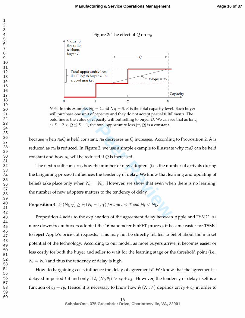
Figure 2: The effect of Q on π0

Note. In this example, NL = 2 and NH = 3. K is the total capacity level. Each buyerwill purchase one unit of capacity and they do not accept partial fulfillments. Thebold line is the value of capacity without selling to buyer B. We can see that as longas K− 2 < Q ≤ K− 1, the total opportunity loss (π0Q) is a constant.

because when π0Q is held constant, π0 decreases as Q increases. According to Proposition 2, δt is

reduced as π0 is reduced. In Figure 2, we use a simple example to illustrate why π0Q can be held

constant and how π0 will be reduced if Q is increased.

The next result concerns how the number of new adopters (i.e., the number of arrivals during

the bargaining process) influences the tendency of delay. We know that learning and updating of

beliefs take place only when Nt = NL. However, we show that even when there is no learning,

the number of new adopters matters to the tendency of delay.

Proposition 4. δt (Nt, γ) ≥ δt (Nt − 1, γ) for any t < T and Nt < NL.

Proposition 4 adds to the explanation of the agreement delay between Apple and TSMC. As

more downstream buyers adopted the 16-nanometer FinFET process, it became easier for TSMC

to reject Apple’s price-cut requests. This may not be directly related to belief about the market

potential of the technology. According to our model, as more buyers arrive, it becomes easier or

less costly for both the buyer and seller to wait for the learning stage or the threshold point (i.e.,

Nt = NL) and thus the tendency of delay is high.

How do bargaining costs influence the delay of agreements? We know that the agreement is

delayed in period t if and only if δt (Nt, θt) > cS + cB. However, the tendency of delay itself is a

function of cS + cB. Hence, it is necessary to know how δt (Nt, θt) depends on cS + cB in order to

16

Page 16 of 37



123456789101112131415161718192021222324252627282930313233343536373839404142434445464748495051525354555657585960

For Peer Review

understand the impact of the bargaining costs. In preparation, we define c∗ = cS + cB as the total

cost of bargaining per period. We then show in the following proposition that as the bargaining

costs increases, agreement delay will be less and less likely.

Proposition 5. δt (Nt, θt) is a decreasing function of c∗ given any possible t, Nt, and θt.

4.3 The Condition for Participation

In the previous section, we investigated the factors that are associated with the tendency of delay

given that the firms have participated in the negotiation. We now study the condition under which

the firms would like to enter the negotiation at the outset. In preparation, we define US0 and UB

0

as the expected payoffs associated with the target capacity for the seller and buyer, respectively,

at the beginning of period 1 given that the firms participate in the negotiation. It is clear that,

US0 + UB

0 = max{

UB1 + US

1 , vQ}− c∗. Additionally, the outside payoffs associated with the target

capacity at the beginning of period 1 are π0γQ for the seller and 0 for the buyer. Hence, the firms

would like to enter into negotiation as long as US0 +UB

0 ≥ π0γQ and if side payments are allowed.

Clearly, if the total value of this transaction is too low, the firms would never start the negotiation

given that negotiation is costly. The following proposition gives a sufficient condition for both

firms to participate.

Proposition 6. If vQ ≥ π0γQ + c∗ and side payments are allowed, firms will negotiate.

Hence, the firms would never negotiate if v is too low and would never delay the agreement

if v is too high. To avoid the trivial case of no participation or no delay, it is sufficient to assume

π0γ +c∗Q≤ v < π0 −

c∗Q

, (8)

which is possible when γ < 1− 2c∗π0Q . Given this condition, it is possible for the firms to achieve a

total expected payoff (US0 + UB

0 ) that is higher than vQ− c∗ and π0γQ by delaying the agreement

and collecting more information during the negotiation because the firms would achieve different

results given different market conditions. If the demand state is known to be “low,” the firms

would reach an agreement and receive a total payoff of vQ minus the bargaining costs; if the de-

mand state is known to be “high,” the bargaining would break down and the firms would receive

17

Page 17 of 37



123456789101112131415161718192021222324252627282930313233343536373839404142434445464748495051525354555657585960

For Peer Review

a total payoff of π0Q minus the bargaining costs. Therefore, in expectation, the total payoff with

more information could be higher than that given by no negotiation or an immediate agreement.

The logic behind the condition for participation also applies to the choice of quitting the ne-

gotiation or staying in any period if quitting is allowed. Details about the choice of quitting will

be discussed in Section 6.4. We will see that firms would never choose to quit if vQ ≥ π0γQ + c∗.

Therefore, agreement delay under this condition is entirely driven by the value of learning.

4.4 The Impact of a Deadline

Due to inflexible production schedules, deadlines often exist for price negotiations. In addition,

in order to avoid stalling or delay of agreements, a commonly used bargaining tactic is to commit

to a deadline (e.g., Moore 2004). Based on previous analyses, we know that firms could benefit

from delay by collecting more information about the market condition. Hence, the existence of a

deadline may hurt the firms that are in such a situation. In this section, we analyze the impact of

a deadline in technology adoption. In particular, we examine how a change in deadline will affect

the firms’ expected payoffs and participation.

In preparation, we assume that π0γ < v < π0, which is weaker than (8). Additionally, let

u0 (T, NL, NH, γ) = US0 + UB

0 denote the joint expected payoff of a bargaining game given that the

deadline is period T, the number of buyers is NL (NH) in an average (a good) market, and the

prior belief about a good market is γ. Recall that US0 + UB

0 = max{

UB1 + US

1 , vQ}− c∗ and that

UB1 + US

1 = E[max

{UB

2 + US2 , vQ

}]− c∗, wherein the expectation is on {N2, θ2}. If we treat the

bargaining game starting from period 2 as a new bargaining game, then the joint expected payoff

of this new bargaining game is thus u0 (T′, N′L, N′H, γ′) = max{

UB2 + US

2 , vQ}− c∗, wherein the

deadline T′ = T− 1, prior belief γ′ = θ2, the total number of adopters in an average market N′L =

NL − N2 + 1, and in a good market N′H = NH − N2 + 1. Therefore, we have u0 (T, NL, NH, γ) =

max {E [u0 (T − 1, NL − N2 + 1, NH − N2 + 1, θ2)] , vQ} − c∗. In particular, for any T ≥ 2,

u0 (T, NL, NH, γ) = −c∗+

max

(

1− α · γ(2−NL)+)· u0 (T − 1, NL, NH, γ) +

α · γ(2−NL)+

· u0

(T − 1, (NL − 2)+ + 1, NH − 1, (1−α)(2−NL)

+·γ

(1−α)(2−NL)+·γ+1−γ

) , vQ

, (9)

18

Page 18 of 37



123456789101112131415161718192021222324252627282930313233343536373839404142434445464748495051525354555657585960

For Peer Review

where x+ = max {0, x}. Now we can analyze how u0 changes with T, using the above iterative

relationship (9) and induction. It reveals that the closer the deadline, the lower the expected payoff

a firm can obtain from participating in the negotiation, which confirms our conjecture.

Proposition 7. u0 (n + 1, NL, NH, γ) ≥ u0 (n, NL, NH, γ) for ∀NL, NH, γ and n ≥ 1.

We then compare our result with those from the literature. On one hand, our model suggests

that the existence of a finite deadline brings inefficiency to the bargaining game and technology

adoption. In this regard, our result is consistent with the literature. On the other hand, our model

offers a new insight regarding how a change in deadline affects firm payoffs. Most studies (e.g.,

Ma and Manove 1993, Fershtman and Seidmann 1993, and Damiano et al. 2012) suggest that

extending a deadline hurts the players because delay is costly and players tend to reach an agree-

ment close to the deadline without bringing additional benefits to the system. However, our

model indicates that extending the deadline benefits the system by better allocating the produc-

tion capacity among buyers with different valuations. Therefore, both negotiating parties can be

better off by extending the deadline if side payments are allowed.

A related question emerges immediately. When are side payments necessary? In other words,

if side payments are not allowed, when will the buyer or supplier suffer from extending the dead-

line? To answer this question, now let’s look at the impact of a deadline from a single firm’s

standpoint. To avoid the trivial cases, we assume that π0γ < v < π0. We then proceed as

follows. First, setting T = 1, we do not allow delay of the agreement. In this case, we know

that UB1 = 0 and US

1 = π0γQ. The transaction price is expected to be p = β min {v, π0γ} +

(1− β)max {v, π0γ} = βπ0γ + (1− β)v and thus the buyer’s (ex ante) expected payoff is UB0 =

(v− p) Q− cB = βQ (v− π0γ)− cB. Next, we allow delay by setting T > 1. Let UB0 (T) denote the

buyer’s expected payoff given a general T. We compare UB0 (T) with UB

0 (T − 1). We find that the

impact of T on UB0 (T) depends on the bargaining power and the seller’s outside option.

Proposition 8. For any T > 1 and π0γ < v < π0, we have UB0 (T) < UB

0 (T − 1) if γπ0Q ≤

(cB − βc∗) /β.

It is immediately observed that γπ0Q ≤ (cB − βc∗) /β holds if β → 0. Hence, given all other

parameters, extending the deadline will hurt the buyer if β is small enough. This is very intu-

itive. When β is too small, the buyer will either pay a very high price (close to v) to purchase the

19

Page 19 of 37



123456789101112131415161718192021222324252627282930313233343536373839404142434445464748495051525354555657585960

For Peer Review

component or receive the outside payoff of zero. In this case, the cost of delay will outweigh the

benefit of learning for the bueyer. Note that this logic also applies to the supplier and thus when

β approaches 1 the supplier will suffer from extending the deadline. Given that the joint payoff

always (weakly) increases with T, the buyer must benefit from extending the deadline when the

supplier suffers.

In addition, an interesting observation is that extending the deadline can hurt the buyer when

the seller has a weak outside option. For example, if cB = cS and β = 1/3, we have UB0 (T) <

UB0 (T − 1) if γπ0Q ≤ cB. Hence, even if the buyer has a decent bargaining power, he cannot ben-

efit from learning if the seller’s expected outside option value is too low. This result is interesting

because in this case we expect the buyer to obtain a significant portion of the surplus as well as the

benefit of learning. However, notice that the buyer can benefit from learning only when they find

that the market is likely to be weak and thus the seller’s opportunity cost (γπ0Q) is weakened.

Given that γπ0Q is low in the first place, the benefit of learning will be marginal for the buyer and

thus will be outweighed by the cost of delay.

Therefore, we learn that the buyer and seller will have a conflict of interest in terms of setting a

deadline when either party has a sufficiently weak bargaining power or when the seller’s expected

opportunity cost and the buyer’s bargaining power are both sufficiently low. When the buyer is

too weak in terms of bargaining power, the seller should use side payments to subsidize the buyer

and set the deadline as far in the future as possible so that the capacity can be better allocated.

Surprisingly, when the initial belief γ for a good market is too low, the seller should also consider

subsidizing the buyer with side payments as long as the seller’s bargaining power is sufficiently

high. If side payments are not allowed and firms are able to commit to an arbitrary deadline prior

to the negotiation, we should expect the negotiation to terminate sooner when these conditions

are satisfied.

4.5 The Time of Agreement

Given that the firms participate in the negotiation and delay is possible, when can the firms even-

tually reach an agreement? To answer this question, let’s first check how the delay tendency is

affected by the length of the negotiation window. We can use Proposition 8 to show that the ten-

20

Page 20 of 37



123456789101112131415161718192021222324252627282930313233343536373839404142434445464748495051525354555657585960

Wei Zhang

Highlight

Wei Zhang

Cross-Out

Wei Zhang

Inserted Text

Proposition 7

For Peer Review

dency of delay in any period increases as the deadline is extended. In other words, the longer

the negotiation window, the more likely the agreement is delayed. In fact, Proposition 9 implies

that if π0γ < v < π0 , we then have δt−1 (Nt, γ) ≥ δt (Nt, γ) for any t < T and Nt < NL. This

is because shortening the negotiation window by one period is equivalent to passing one period

without observing a new adopter and without updating the belief.

Proposition 9. Given that π0γ < v < π0, δt (Nt, θt) is an increasing function of T given any possible t,

Nt, and θt.

Combining all the previous propositions, we arrive at two conclusions. First, reaching an

agreement is possible in any period t ≤ T. If the agreement cannot be reached in the first period,

the delay tendency can be weakened as time passes and thus the agreement can be reached in any

subsequent period. Second, agreements—if not reached at the beginning, are likely to be reached

after some periods of learning. Although Proposition 9 suggests that the tendency of delay can be

weakened over time, this effect will be reduced or even eliminated according to Proposition 4 as

new adopters appear. Once the critical point is reached, the learning starts and the delay tendency

will be continually reduced conditioning on that the bargaining does not break down. Therefore,

the overall pattern of the frequency of agreement should be “U”-shaped, which is supported by

our simulations.

5 Numerical Examples and Simulation

Through theoretical analysis, we understand that the delay of agreement in our model is driven

by the benefit of learning about the demand, and that the tendency of delay can be influenced by a

number of factors. Here we try to use numerical examples to gain a better understanding of how

the bargaining actually proceeds under different parameter settings and calculate the expected

payoffs. To this end, we first use a large number of random instances to simulate the bargaining

process given that the participation condition is strictly satisfied. Second, we investigate how the

firms’ respective expected payoffs, UB0 and US

0 (as well as UB0 + US

0 ) change with the parameters.

In our numerical examples, the default parameter setting is as follows: π0 = 10, v = 6, α = 0.5,

β = 0.5, γ = 0.4, Q = 1, NL = 5, cS = cB = 0.01, and T = 10.

21

Page 21 of 37



123456789101112131415161718192021222324252627282930313233343536373839404142434445464748495051525354555657585960

For Peer Review

In the first study, we examine eight different parameter settings. We generate 1,000 random

instances for each setting and plot a histogram showing the distribution of the time of termination

(i.e., agreement or breakdown). For the simulation, we build a tree of all the possible results of the

game under a fixed parameter setting, calculate the expected no-agreement payoffs at each node

of the tree, and generate random market conditions and buyer arrivals to obtain “sample paths”

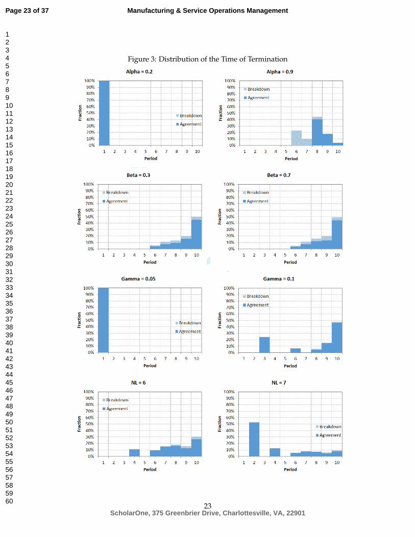
of the game. The results are presented in Figure 3. In aggregate, an interesting observation is that,

in most cases, the agreement is either reached in the first few periods or close to the deadline,

depending on the parameter setting. This observation is consistent with the result of Propositions

2, 3 and 4: the tendency of delay increases as more buyers arrive and an agreement can be achieved

only when belief of a good market becomes low enough through learning. We particularly test the

impact of α, β, γ, and NL.

The time of agreement is influenced by α (i.e., the probability of a new arrival given that the

arrival process is still on) in a non-monotonic way. When α is low (= 0.2), the agreement is always

reached in period 1, because the low arrival rate of buyers makes it costly to learn about the

demand given a fixed cost of bargaining per period. When the benefit of learning is low, firms can

reach agreement immediately. In contrast, a higher α (= 0.5, as shown in the second row of Figure

3) allows easier learning and thus delay occurs. As α becomes larger, the time of agreement shifts

rapidly from the first few periods to the last few periods, skipping periods in the middle. If we

combine the instances under different parameter settings, the distribution should be U-shaped.

Interesting, when α is extremely large (=0.9), the time of agreement is shifted forward, because the

learning is highly effective when α is extremely large, and thus the firms do not need to wait as

long to learn about the demand.

From the second row of Figure 3, we can see that β (i.e., the relative bargaining power of the

buyer) has little impact on the bargaining process other than determining the split of the surplus.

As a result, the second row of Figure 3 in fact serves as the baseline scenario with the default

parameter setting. Next, from the second and third rows, we can see that the agreement becomess

delayed for longer periods as the prior belief (γ) of a good market increases, which is consistent

with Proposition 3. Lastly, from the second and fourth rows, we can see that as the non-learning

period (i.e., there is no learning when Nt < NL) becomes longer, the agreement occurs sooner,

because the length of the non-learning period indicates the cost of learning.

22

Page 22 of 37



123456789101112131415161718192021222324252627282930313233343536373839404142434445464748495051525354555657585960

For Peer Review

Figure 3: Distribution of the Time of Termination

23

Page 23 of 37



123456789101112131415161718192021222324252627282930313233343536373839404142434445464748495051525354555657585960

For Peer Review

Figure 4: Impact of Different Parameters on UB0 , US

0 , and UB0 + US

0

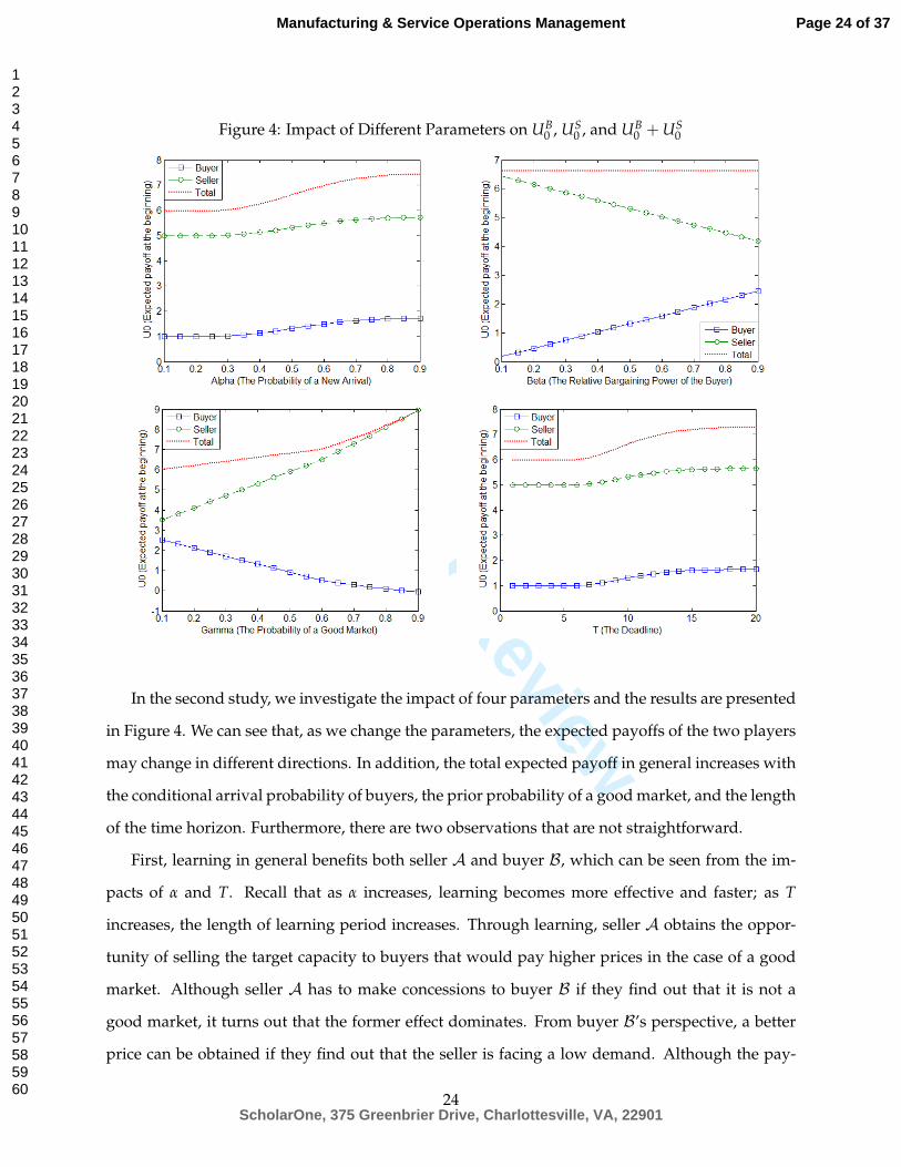
In the second study, we investigate the impact of four parameters and the results are presented

in Figure 4. We can see that, as we change the parameters, the expected payoffs of the two players

may change in different directions. In addition, the total expected payoff in general increases with

the conditional arrival probability of buyers, the prior probability of a good market, and the length

of the time horizon. Furthermore, there are two observations that are not straightforward.

First, learning in general benefits both seller A and buyer B, which can be seen from the im-

pacts of α and T. Recall that as α increases, learning becomes more effective and faster; as T

increases, the length of learning period increases. Through learning, seller A obtains the oppor-

tunity of selling the target capacity to buyers that would pay higher prices in the case of a good

market. Although seller A has to make concessions to buyer B if they find out that it is not a

good market, it turns out that the former effect dominates. From buyer B’s perspective, a better

price can be obtained if they find out that the seller is facing a low demand. Although the pay-

24

Page 24 of 37



123456789101112131415161718192021222324252627282930313233343536373839404142434445464748495051525354555657585960

For Peer Review

off is zero for buyer B in a good market, the expected payoff is still higher than that of without

learning. (In a simple example wherein Q = 1, β = 0.5, and c∗ = 0, the buyer’s expected payoff

is v− (v + π0γ) /2 without learning and (1− γ) v/2 with learning. Clearly, the expected payoff

with learning is higher if π0 > v.) Based on this observation, we know that both the seller and

buyer should prefer a longer time horizon over a shorter one. In addition, neither party needs to

compensate each other for a longer horizon or extending the deadline. As a result, a committed

deadline in such a setting is not credible.

The second important observation is that participation is possible even if γ (i.e., the prior

probability of a good market) is relatively high such that π0γ > v and the sufficient condition of

participation is violated. Therefore, bargaining and learning “on the go” can take place for a wide

range of scenarios, which means that our results can be widely applied.

6 Extensions and Discussions

In this section, we present four extensions of our base model to incorporate a number of realistic

but complicating factors. We will see that the results will not be qualitatively different from what

is offered by the base model. Hence, the robustness of the base model will be supported by the

analyses of these extensions.

6.1 State-Dependent Value of Technology

Due to the network effect in a high technology market, it is likely that the value of a unit of ca-

pacity for the buyer is vH in a good market and is vL in an average market, where vH > vL.

In such a setting, the expected product value in period t, given information {Nt, θt}, is vet =

θtvH + (1− θt) vL = vL + (vH − vL) θt. Therefore, an agreement can be reached in period t if and

only if USt + UB

t ≤ vet Q, or equivalently, US

t + UBt − (vH − vL) θtQ ≤ vLQ. Based on this criterion,

we can define the following equivalent bargaining game.

Consider a bargaining game wherein the value of a unit of the capacity for buyer B is fixed

at vL and the seller’s opportunity loss for a unit of the target capacity in a good market is π∗ =

π0 − (vH − vL). All of the other settings are the same as those in the base model. We can prove

that, in terms of the time when an agreement can be achieved, this bargaining game is completely

25

Page 25 of 37



123456789101112131415161718192021222324252627282930313233343536373839404142434445464748495051525354555657585960

For Peer Review

equivalent to bargaining with network-based product value. Consequently, all the results in the

base model can apply.

Proposition 10. USt + UB

t ≤ vet Q given {π0, ve

t} is equivalent to USt + UB

t ≤ vLQ given {π∗, vL} and

USt + UB

t = USt + UB

t + (vH − vL) θtQ for every possible t.

Similarly, the value of technology for the buyer could be market-condition-dependent due to

the competition among the buyers. It is sometimes reasonable to expect that the more adopters for a

technology, the more intense the competition and thus the lower the profit margin. Hence, for the

focal buyer, the per-unit value could be vH in a good market and is vL in an average market, where

vH < vL. Despite this difference, all the above arguments as well as the results can be carried over.

6.2 The Leader-Follower Effect

It is possible that in the high-tech industry, the adoption decision of a market leader could influ-

ence those of other firms in the same market segment. For example, in the microprocessor market

for smartphones, buyers such as Apple, Qualcomm, and Nvidia can choose between the process

technologies offered by Samsung and TSMC, and their adoption decisions are mainly driven by

Apple (Lipsky 2016).

Here we study the situation wherein the state of demand depends on whether an agreement

is reached between A and B. In particular, if the market condition is initially good, the agreement

will have no effect; however, if the market is initially average, the agreement between A and B in

any period can turn the market into a good one with probability φ. Let γ denote the original prob-

ability of a good market and θt the probability of a good market in period t without an agreement.

After an agreement is reached in period t, the probability of a good market becomes θt +(1− θt) φ.

Accordingly, the value of an agreement between A and B is twofold. First, the value of Q units of

the capacity for the buyer is vQ. Second, the agreement can increase the probability of a good mar-

ket and thus the probability of selling the extra capacity of K− Q− (NL − 1) units is raised from

θt to θt + (1− θt) φ in period t. Let πe denote the value of the extra capacity for the seller in a good

market when it is sold to other buyers. Hence, the total value of the agreement is vQ+(1− θt) φπe,

and an agreement can be reached in period t if and only if USt +UB

t ≤ vQ + (1− θt) φπe, or equiv-

alently, USt + UB

t + πeφQ θtQ ≤

(v + πeφ

Q

)Q. Based on this criterion, we can define the following

26

Page 26 of 37



123456789101112131415161718192021222324252627282930313233343536373839404142434445464748495051525354555657585960

For Peer Review

equivalent bargaining game in a way similar to Section 6.1.

Consider a bargaining game wherein the value of a unit of the capacity for buyer B is fixed at

vl f e = v + πeφQ and the seller’s opportunity loss for a unit of the target capacity in a good market

is πl f e = π0 +πeφQ . All of the other settings are the same as those used in the base model. Using

the same logic as in Proposition 10, we can show that, in terms of the time when an agreement

can be achieved, this bargaining game is completely equivalent to the bargaining game with the

leader-follower effect. The proof is omitted. All of the results in the base model can apply.

6.3 Adoption by Customer Groups

In practice, potential customers can usually be classified into several types in terms of the likeli-

hood of adoption. Although the base model is reasonable if the seller does not know the type of a

buyer a priori, when the type information is known for all of the buyers, a reasonable assumption

for capturing market uncertainty in our model is that two types of buyers exist: strategic partners

and market followers. It is certain that strategic partners will adopt the technology. Market fol-

lowers will all adopt the technology if they think it is promising, which is true with probability γ.

Given this assumption, firms can be sure that the market condition is good if one of the market

followers decides to adopt the technology. To incorporate such a situation, we can just assume

that NL buyers have arrived by period 0 (or equivalently, NL = 1), and the learning about the

market condition starts immediately in period 1. Hence, the same results as in the base model can

apply.

6.4 The Option of Quitting

Proposition 7 gives us a sufficient condition under which the two parties will participate in the

negotiation. Note that when the firms fail to reach an agreement in a period, it is equivalent that

they participate in a new negotiation starting from the next period with the prior information as

the current information. Therefore, Proposition 7 also gives a sufficient condition under which

the firms will not choose to quit the negotiation in period t even if quitting is allowed, except that

the “prior information” γ should be replaced by θt. In particular, if vQ ≥ π0θtQ + c∗ and side

payments are allowed, firms will not quit in period t. Note that θt ≤ γ as long as Nt ≤ NL. Hence,

27

Page 27 of 37



123456789101112131415161718192021222324252627282930313233343536373839404142434445464748495051525354555657585960

For Peer Review

if π0γ < v < π0 and vQ ≥ π0γQ+ c∗, firms will never quit unless agreement becomes impossible.

6.5 State-Dependent Arrivals

In the base model, we assume that the probability of a new adopter arriving in each period (given

that Nt ≤ N) is constant regardless of the market condition. Given this assumption, learning

occurs at a critical point (i.e., when Nt = NL), where the firms either find the demand to be high

for sure or update the belief θt downwards. An alternative assumption is that the probability of a

new arrival is different under different market conditions. In particular, the probability is αL in an

average market and αH in a good market, wherein αL < αH. Given this assumption, learning starts

from the very beginning. As time passes, the belief θt could be updated upwards or downwards.

It is reasonable to expect that there exist a pair of critical values, θ∗t and θ∗t , such that the bargaining

breaks down when θt ≥ θ∗t , an agreement is reached when θt ≤ θ∗t , and the agreement is delayed

when θ∗t < θt < θ∗t . Hence, the insights of such a model regarding agreement delay will be the

same as what are offered by the base model. In fact, the insights we obtained from the base model

are independent of the learning mechanism, but the base model offers great tractability.

7 Concluding Remarks

In this paper, we study the negotiation process between a high-technology component supplier

and an OEM buyer. We focus on a setting wherein the buyer decides to adopt the technology

offered by the supplier for the next generation of product and has determined the production

plan of the final product as well as the purchase quantity of the focal component. Therefore, the

buyer’s only task is to negotiate with the supplier for the price before a fixed deadline. Observa-

tions in the semiconductor industry suggest that when the manufacturing capacity is fixed and

demand is uncertain, firms can delay the price agreement until close to the deadline even if they

have symmetric information. To find the rationale of delay as well as the managerial insights in

such a setting, we build a dynamic bargaining model with random price proposers, fixed bargain-

ing and delay costs, uncertain outside options, symmetric information, and a deadline. Using the

model, we discover that delay of agreements is driven by the incentive to learn about the sup-

plier’s opportunity cost of selling, which is jointly determined by the demand facing the supplier

28

Page 28 of 37



123456789101112131415161718192021222324252627282930313233343536373839404142434445464748495051525354555657585960

For Peer Review

and the level of capacity. When the demand is high (low), the opportunity cost of selling to the

buyer is high (low). With better information, the supplier can sell the manufacturing capacity to

buyers who are expected to pay more. On the other hand, the buyer can also benefit from learning

because the supplier must make consessions if they find that the demand is likely to be weak.

Hence, contrary to most existing theories, delay can benefit both the supplier and buyer and the

joint expected payoff always weakly increases as the deadline is extended. This logic holds even

if we allow the value of the capacity to depend on the market condition or extend the model in a

number of other ways.

We also point out that extending the deadline or a long negotiation window is not always a

common interest for the buyer and supplier. Although extending the deadline can improve the

joint payoff, close deadlines are preferred by the buyer when the buyer has a sufficiently low

bargaining power or when the supplier with a strong bargaining power is very likely to have

excessive capacities. Therefore, when the buyer is too weak in terms of bargaining power, the

supplier should use side payments to subsidize the buyer and set the deadline as far in the fu-

ture as possible so that the capacity can be better allocated. Surprisingly, when the initial belief

for a good market is too low, the supplier should also consider subsidizing the buyer with side

payments as long as the supplier’s bargaining power is sufficiently high. If side payments cannot

be used and firms are able to commit to an arbitrary deadline prior to the negotiation, we should

expect the negotiation to terminate quickly when these conditions are satisfied.

In addition, our model suggests that the tendency of delay decreases as time passes and in-

creases with the expected value of the supplier’s outside option, the number of buyers that have

decided to adopt the technology, and the bargaining time horizon. Based on these results, our

model predicts that agreements are frequently achieved either at the beginning of negotiations or

close to the deadlines. This is consistent with the “deadline effect” as documented in the litera-

ture (e.g., Roth et al. 1988, Fershtman and Seidmann 1993, and Damiano et al. 2012). However,

our model offers a new explanation; that is, given that the incentive to learn is high enough at

the outset, the delay tendency will be reduced below the threshold for an agreement only after a

long-enough period of time.

One way to test the theory in this paper is to test the correlation between the chance of delay

and the length of the negotiation window. Most existing theories should predict no correlation

29

Page 29 of 37



123456789101112131415161718192021222324252627282930313233343536373839404142434445464748495051525354555657585960

For Peer Review

or a negative correlation because delay should not increase the joint payoff. However, our theory

predicts a positive correlation because longer negotiation windows allow better learning and a

higher joint payoff. Future research can consider testing the importance of learning in technology

adoption along this direction.

References

[1] Admati AR, Perry M (1987) Strategic Delay in Bargaining. Review of Economic Studies54(3):345–364.

[2] Aydin G, Heese HS (2015) Bargaining for an Assortment. Management Science 61(3):542–559.

[3] Bass FM (1969) A New Product Growth Model for Consumer Durables. Management Science15(5) 215–227.

[4] Binmore K (1987) Perfect Equilibria in Bargaining Models. The Economics of Bargaining (K.Binmore and P. Dasgupta, Eds.), Blackwell, Oxford.

[5] Binmore K, Robinstein A, Wolinsky A (1986) The Nash Bargaining Solution in EconomicModelling. RAND J. of Economics 17(2):176–188.

[6] Cai H (2000) Delay in Multilateral Bargaining under Complete Information. Journal of Eco-nomic Theory 93(2):260–276.

[7] Clover J (2015) A9 Chip Manufacturing Split 60/40 Between TSMC andSamsung, Not Segmented by Device Size. MacRumors (September 29),http://www.macrumors.com/2015/09/29/a9-chip-split-tsmc-samsung/.

[8] Cramton PC (1984) Bargaining with Incomplete Information: An Infinite-Horizon Modelwith Two-Sided Uncertainty. Review of Economic Studies 51(4):579–593.

[9] Cramton PC (1992) Strategic Delay in Bargaining with Two-Sided Uncertainty. Review of Eco-nomic Studies 59(1):205–225.

[10] Damiano E, Li H, Suen W (2012) Optimal Deadlines for Agreements. Theoretical Economics7(2):357–393.

[11] Dukes AJ, Gal-Or E, Srinivasan K (2006) Channel Bargaining with Retailer Asymmetry. Jour-nal of Marketing Research 43(1):84–97.

[12] Feng Q, Lai G, Lu LX (2015) Dynamic Bargaining in a Supply Chain with Asymmetric De-mand Information. Management Science 61(2):301–315.

30

Page 30 of 37



123456789101112131415161718192021222324252627282930313233343536373839404142434445464748495051525354555657585960

For Peer Review

[13] Fershtman C, Seidmann DJ (1993) Deadline Effects and Inefficient Delay in Bargaining withEndogenous Commitment. Journal of Economic Theory 60(2):306–321.

[14] Fuchs W, Skrzypacz A (2010) Bargaining with Arrival of New Traders. American EconomicReview 100(3):802–836.

[15] Guo L, Iyer G (2013) Multilateral Bargaining and Downstream Competition. Marketing Science32(3):411–430.

[16] Ho TH, Savin S, Terwiesch C (2002) Managing Demand and Sales Dynamics in New ProductDiffusion under Supply Constraint. Management Science 48(2):187–206.

[17] Hughes N (2015) Apple makes ’last-minute decision’ to use TSMC for 30% of ’A9’ chip ordersfor next iPhone. AppleInsider (April 15), http://appleinsider.com/articles/15/04/15/apple-makes-last-minute-decision-to-use-tsmc-for-30-of-a9-chip-orders -for-next-iphone/.

[18] Jensen R (1982) Adoption and Diffusion of an Innovation of Uncertain Profitability. Journal ofEconomic Theory 27(1):182–193.

[19] Karabuk S, Wu SD (2003) Coordinating Strategic Capacity Planning in the SemiconductorIndustry. Operations Research 51(6):839–849.

[20] Krishnan TV, Bass FM, Jain DC (1999) Optimal Pricing Strategy for New Products. Manage-ment Science 45(12):1650–1663.

[21] Kumar S, Swaminathan JM (2003) Diffusion of Innovations under Supply Constraints. Oper-ations Research 51(6):866–879.

[22] Li D (2007) Bargaining with History-Dependent Preferences. Journal of Economic Theory136(1):695–708.

[23] Lien J, Shen J (2015) TSMC says 16nm ramp on schedule. DigiTimes (August 11),http://www.digitimes.com/news/a20150811PD217/.

[24] Lipsky J (2016) FinFETs Flow at Samsung, TSMC. EE Times (Feburary 3),http://www.eetimes.com/document.asp?doc_id=1328852/.

[25] Lovejoy WS (2010) Bargaining Chains. Management Science 56(12):2282–2301.

[26] Luk L (2014) TSMC Starts Shipping Microprocessors to Apple. The Wall Street Journal (July 10),http://www.wsj.com/articles/tsmc-starts-shipping-microprocessors-to-apple-1404991514/.

[27] Ma CA, Manove M (1993) Bargaining with Deadlines and Imperfect Player Control. Econo-metrica 61(6):1313–1339.

[28] McCardle KF (1985) Information Acquisition and the Adoption of New Technology. Manage-ment Science 31(11):1372–1389.

31

Page 31 of 37



123456789101112131415161718192021222324252627282930313233343536373839404142434445464748495051525354555657585960

For Peer Review

[29] Moore DA (2004) Deadline Pressure: Use It to Your Advantage. Negotiation 7(8).

[30] Muthoo A (1999) Bargaining Theory with Applications. Cambridge University Press, Cam-bridge, UK.

[31] Nagarajan M, Bassok Y (2008) A Bargaining Framework in Supply Chains: The AssemblyProblem. Management Science 54(8):1482–1496.

[32] Nash J (1950) The Bargaining Problem. Econometrica 18(2):155–162.

[33] Robinson B, Lakhani C (1975) Dynamic Price Models for New Product Planning. ManagementScience 21(10):1113–1122.

[34] Robinstein A (1982) Perfect Equilibrium in a Bargaining Model. Econometrica 50(1):97–110.

[35] Roth AE, Murnighan JK, Schoumaker F (1988) The Deadline Effect in Bargaining: Some Ex-perimental Evidence. American Economic Review 78(4):806–823.

[36] Shen W, Duenyas I, Kapuscinski R (2011) New Product Diffusion Decisions Under SupplyConstraints. Management Science 57(10):1802–1810.

[37] Shilov A (2015) Nvidia and Samsung still cannot finalize chip manufacturing deal. Kit-Guru (June 20), http://www.kitguru.net/components/graphic-cards/anton-shilov/nvidia-and-samsung-still-cannot-finalize-chip-manufacturing-deal/.

[38] Singh J (2015) Samsung in talks with Apple to supply OLED displays for future iPhones. In-ternational Business Times (November 14), http://www.ibtimes.co.uk/samsung-talks-apple-supply-oled-displays-future-iphones-1528717/.

[39] Ungureanu H (2016) Samsung Reportedly Making 100 MillionOLED Displays For Apple’s iPhone 7s Plus. Tech Times (April 16),http://www.techtimes.com/articles/150568/20160416/samsung-reportedly-making-100-million-oled-displays-for-apples-iphone-7s-plus.htm.

[40] Zhang W, Dasu S, Ahmadi R (2016) Higher Prices for Larger Quantities? Non-MonotonicPrice-Quantity Relations in B2B Markets. Management Science, forthcoming.

32

Page 32 of 37



123456789101112131415161718192021222324252627282930313233343536373839404142434445464748495051525354555657585960

For Peer Review

Supplementary to “Demand Learning and Agreement Delay in Tech-

nology Adoption”

Proof of Proposition 1

There are two special cases. First, if Nt > NL, there is no uncertainty. Thus, either an agreement

is reached or the bargaining breaks down. Second, in period T, an agreement must be reached or

the bargaining breaks down. Let’s then consider Nt ≤ NL for period t < T. In period T − 1, we

have UBT−1 + US

T−1 ≤ Q ·max {π0, v} − cS − cB. If vQ + cS + cB ≥ π0Q, then we have UBT−1 +

UST−1 ≤ max {vQ + cS + cB, vQ} − cS − cB = vQ. Suppose now UB

t + USt ≤ vQ. For period t− 1,

we have UBt−1 + US

t−1 = E[max

{UB

t + USt , vQ

}|Nt, θt

]− cS − cB ≤ vQ− cS − cB < vQ. �


From Table-2, we know that UBT +US

T increases with π0. Because δt = UBt +US

t + cS + cB− vQ,

we know that δT increases with π0. Now suppose that δt+1 increases with π0. According to (6),

δt = E [max {0, δt+1 − cS − cB}], which is an increasing function of δt+1 and thus π0. �


First consider that Nt = NL. We have δT−1 = Q ·max {π0θT−1 − v, αθT−1 (π0 − v)} and it is

increasing in θT−1. Suppose that δt (NL, θt) is increasing in θt for a t. Using (6), we have

δt−1 (NL, θt−1) =θt−1α (π0 − v) Q + (1− θt−1α)max{

δt

(NL,

(1− α)θt−1

1− αθt−1

)− cS − cB, 0

}.

For any θ′ > θ′′, we have δt

(NL, (1−α)θ′

1−αθ′

)≥ δt

(NL, (1−α)θ′′

1−αθ′′

)and thus

δt−1(

NL, θ′)− δt−1

(NL, θ′′

)≥(θ′ − θ′′

)α (π0 − v) Q +

(θ′′ − θ′

)α max

{δt

(NL,

(1− α)θ′′

1− αθ′′

)− cS − cB, 0

}≥(θ′ − θ′′

)α (π0Q− vQ− δt + cS + cB)

=(θ′ − θ′′

)α(

π0Q−UBt −US

t

)≥ 0.

Hence, δt (Nt, θt) is increasing in θt for any t given Nt = NL. Next, consider that Nt < NL, which

33

Page 33 of 37



123456789101112131415161718192021222324252627282930313233343536373839404142434445464748495051525354555657585960

For Peer Review

suggests that θt ≡ γ. We have δT−1 (NT−1, γ) = Q ·max {0, π0γ− v} and it is increasing in γ for

any NT−1 < NL. Now suppose that δt (Nt, γ) is increasing in γ for any Nt < NL. Using (6), we get

δt−1 (Nt−1, γ) = (1− α)max {0, δt (Nt−1, γ)− cS − cB}+ α max {0, δt (Nt−1 + 1, γ)− cS − cB} .

Clearly, δt−1 (Nt−1, γ) is increasing in γ given that δt (Nt, γ) is increasing in γ for any Nt ≤ NL.

The proof is complete. �


We know that θt ≡ γ for Nt < NL. In period T − 1, δT−1 (NT−1 − 1, γ) = δT−1 (NT−1, γ) =

Q ·max {0, π0γ− v}. Now suppose δt (Nt, γ) ≥ δt (Nt − 1, γ) in period t. Then in period t− 1,

δt−1 (Nt−1 − 1, γ) = (1− α)max {0, δt (Nt−1 − 1, γ)− cS − cB}+ α max {0, δt (Nt−1, γ)− cS − cB}

≤ (1− α)max {0, δt (Nt−1, γ)− cS − cB}+ α max {0, δt (Nt−1 + 1, γ)− cS − cB}

=δt−1 (Nt−1, γ) .

Hence, the inequality applies to every t < T. The proof is complete. �


First, we know from Table 2 that δT−1 (NT−1, θT−1) is independent of c∗ for any NT−1 and

θT−1. In other words, δT−1 is weakly decreasing in c∗. Then according to the definition in (6),

δt (c∗) = E [max {0, δt+1(c∗)− c∗}]. Hence, if δt+1 is (weakly) decreasing in c∗, then δt must be (at

least weakly) decreasing in c∗. �


If the firms choose to agree on a price immediately, they can achieve at least a total payoff of

vQ− c∗; i.e., US0 + UB

0 ≥ vQ− c∗. Hence, if vQ ≥ π0γQ + c∗, we have US0 + UB

0 ≥ (π0γQ + c∗)−

c∗ = π0γQ. �


For the ease of notation, we write u0 (n, NL, NH, γ) as un0 . First, according to Table 2, we have

34

Page 34 of 37



123456789101112131415161718192021222324252627282930313233343536373839404142434445464748495051525354555657585960

For Peer Review

u10 = Q ·max {π0γ, v} − c∗ = vQ− c∗, u2

0 = vQ− c∗ + max {0, Qαγ (π0 − v)− c∗} if NL = 1, and

u20 = vQ− c∗ if NL > 1. Therefore, we must have u2

0 ≥ u10 for ∀NL, NH, γ. Second, suppose that

un0 ≥ un−1

0 for a particular n ≥ 2 and ∀NL, NH, γ. In the third step, we can show that un+10 ≥ un

0

using (9). This is because u0 (n, NL, NH, γ) ≥ u0 (n− 1, NL, NH, γ) and u0 (n, NL − 1, NH − 1, γ) ≥

u0 (n− 1, NL − 1, NH − 1, γ) according to the assumption made in the second step. The proof is

complete. �


We first check T = 2. In this case, UB2 = 0 and US

2 = θ2π0Q ≥ 0. According to Table 1, we

know that given T = 2

UB1 + US

1 =

Q ·max {π0γ, v} − c∗ N1 < NL

Q ·max {π0γ, v + αγ (π0 − v)} − c∗ N1 = NL

and thus

UB0 (2) =β max

{UB

1 , vQ−US1

}+ (1− β)UB

1 − cB

=

β max

{UB

1 , UB1 + c∗

}+ (1− β)UB

1 − cB N1 < NL

β max{

UB1 , UB

1 + c∗ − αγQ (π0 − v)}+ (1− β)UB

1 − cB N1 = NL

≤UB1 + βc∗ − cB

Using (2) and knowing that θ2 ≥ (1−α)γ1−αγ and Pr

{θ2 = (1−α)γ

1−αγ

}< 1, we have

UB1 =E [βQ max {0, v− θ2π0}+ (1− β) · 0]− cB

<βQ(

v− π0 ·(1− α)γ

1− αγ

)− cB

=UB0 (1) + βQπ0 ·

αγ(1− γ)

1− αγ.

Hence, UB0 (2) < UB

0 (1) + βQπ0 · αγ(1−γ)1−αγ + βc∗ − cB. Therefore, βQπ0 · αγ(1−γ)

1−αγ + βc∗ − cB ≤ 0 or

Qπ0 · αγ(1−γ)1−αγ ≤ (cB − βc∗) /β is a sufficient condition under which UB

0 (2) < UB0 (1). We know

that α(1−γ)1−αγ ≤ 1, so Qπ0γ ≤ (cB − βc∗) /β is a sufficient condition under which UB

0 (2) < UB0 (1).

35

Page 35 of 37



123456789101112131415161718192021222324252627282930313233343536373839404142434445464748495051525354555657585960

For Peer Review

Next, let’s suppose that for T = m and π0γ < v < π0 we have UB0 (m) < UB

0 (m− 1) if

Qπ0γ ≤ (cB − βc∗) /β. We then consider the case of T = m + 1. Using Proposition 8, we know

that UB1 (m + 1) + US

1 (m + 1) ≥ UB1 (m) + US

1 (m). Hence,

UB0 (m + 1) =β max

{UB

1 (m + 1) + US1 (m + 1) , vQ

}− βUS

1 (m + 1) + (1− β)UB1 (m + 1)− cB

=β[vQ−UB

1 (m + 1)−US1 (m + 1)

]++ UB

1 (m + 1)− cB

≤β[vQ−UB

1 (m)−US1 (m)

]++ UB

1 (m + 1)− cB

=β[vQ−UB

1 (m)−US1 (m)

]++ UB

1 (m)−UB1 (m) + UB

1 (m + 1)− cB

=UB0 (m)−UB

1 (m) + UB1 (m + 1) .

Notice that UB1 (m + 1) = E

[UB

0 (m)], where UB

0 (m) denotes the buyer’s expected payoff in a

hypothetical negotiation where γ = θ2 and N1 = N2 with θ2 and N2 being the period-2 information

in the focal negotiation. We know that we either have θ2 = 1 or θ2 ≤ γ. In the former case, it is clear

that UB0 (m) = 0 regardless of the value of m. In the latter case, we have Qπ0θ2 ≤ (cB − βc∗) /β

and thus UB0 (m) < UB

0 (m− 1). Therefore, if Qπ0γ ≤ (cB − βc∗) /β, we have UB1 (m + 1) =

E[UB

0 (m)]< E

[UB

0 (m− 1)]= UB

1 (m). Consequently, we have UB0 (m + 1) < UB

0 (m) if Qπ0γ ≤

(cB − βc∗) /β.�


We know that δt (Nt, θt) = UBt (Nt, θt) + US

t (Nt, θt) + c∗ − vQ and that c∗ and vQ are indepen-

dent of T. In addition, for any T − t > 1 and Nt < NL, we have

UBt (Nt, θt) + US

t (Nt, θt) =E[max

{UB

t+1 + USt+1, vQ

}− c∗|Nt, θt

]=E [u0 (T − t− 1, NL − Nt+1 + 1, NH − Nt+1 + 1, θt+1) |Nt, θt] ,

wherein u0 is the expected total payoff in an equivalent game that is parameterized by T′ = T −

t− 1, N′L = NL − Nt+1 + 1, N′H = NH − Nt+1 + 1, and γ′ = θt+1. The proof is then completed by

Proposition 8. �


36

Page 36 of 37



123456789101112131415161718192021222324252627282930313233343536373839404142434445464748495051525354555657585960

For Peer Review

In period T, we know UST + UB

T = π0θTQ and thus UST + UB

T ≤ veTQ is equivalent to π0θTQ ≤

[vL + (vH − vL) θT] Q, which is simply UST + UB

T = π∗θTQ ≤ vLQ. Clearly, UST + UB

T = UST + UB

T +

(vH − vL) θTQ. Now suppose that the two bargaining games are equivalent for any period t ≥ t′

and USt′ + UB

t′ = USt′ + UB

t′ + (vH − vL) θt′Q. We then consider period t′ − 1. With network-based

product value, we have

USt′−1 + UB

t′−1 =E[max{

UBt′ + US

t′ , vet′Q}]− c∗

=E[max{

UBt′ + US

t′ + (vH − vL) θt′Q, vet′Q}]− c∗

=E[max{

UBt′ + US

t′ , vLQ}]− c∗ + (vH − vL) θt′−1Q.

Therefore, USt′−1 + UB

t′−1 ≤ vet′−1Q is equivalent to E[max

{UB

t′ + USt′ , vLQ

}]− c∗ = UB

t′−1 + USt′−1 ≤

vet′−1Q− (vH − vL) θt′−1Q = vLQ. �

37

Page 37 of 37



123456789101112131415161718192021222324252627282930313233343536373839404142434445464748495051525354555657585960

For Peer Review - USC Marshall · For Peer Review Demand Learning and A greement Delay in...

Documents

Transcript of For Peer Review - USC Marshall · For Peer Review Demand Learning and A greement Delay in...