Foody, Giles M. (1996) Approaches for the production and ...

Foody, Giles M. (1996) Approaches for the production and evaluation of fuzzy land cover classifications from remotely sensed data. International Journal of Remote Sensing, 17 (7). pp. 1317-1340. ISSN 0143-1161

Access from the University of Nottingham repository: http://eprints.nottingham.ac.uk/2276/1/ePrints-2014-ijrs96.pdf

Copyright and reuse:

The Nottingham ePrints service makes this work by researchers of the University of Nottingham available open access under the following conditions.

This article is made available under the University of Nottingham End User licence and may be reused according to the conditions of the licence. For more details see: http://eprints.nottingham.ac.uk/end_user_agreement.pdf

A note on versions:

The version presented here may differ from the published version or from the version of record. If you wish to cite this item you are advised to consult the publisher’s version. Please see the repository url above for details on accessing the published version and note that access may require a subscription.

For more information, please contact [email protected]

mailto:[email protected]

Approaches for the production and evaluation of fuzzy land cover classifications from remotely sensed data

Foody, G. M.

International Journal of Remote Sensing, 17, 1317-1340 (1996)

The manuscript of the above article revised after peer review and submitted to the journal for publication, follows. Please note that small changes may have been made after submission and the definitive version is that subsequently published as:

Foody, G.M., 1996. Approaches for the production and evaluation of fuzzy land cover classifications from remotely sensed data, International Journal of Remote Sensing, 17, 1317-1340.

Approaches for the production and evaluation of fuzzy land cover classifications from remotely sensed data.

Giles M. Foody Department of Geography University of Wales Swansea Singleton Park Swansea SA2 8PP UK

Running headline: Fuzzy classification approaches and evaluation

Submitted for publication in the International Journal of Remote Sensing. (Revised manuscript - Paper RES 120035)

2

Abstract

Remote sensing is an attractive source of data for land cover mapping applications.

Mapping is generally achieved through the application of a conventional statistical

classification, which allocates each image pixel to a land cover class. Such approaches are

inappropriate for mixed pixels, which contain two or more land cover classes, and a fuzzy

classification approach is required. When pixels may have multiple and partial class

membership measures of the strength of class membership may be output and, if strongly

related to the land cover composition, mapped to represent such fuzzy land cover. This

type of representation can be derived by softening the output of a conventional 'hard'

classification or using a fuzzy classification. The accuracy of the representation provided

by a fuzzy classification is, however, difficult to evaluate. Conventional measures of

classification accuracy cannot be used as they are appropriate only for 'hard' classifications.

The accuracy of a classification may, however, be indicated by the way in which the

strength of class membership is partitioned between the classes and how closely this

represents the partitioning of class membership on the ground. In this paper two measures

of the closeness of the land cover representation derived from a classification to that on the

ground were used to evaluate a set of fuzzy classifications. The latter were based on

measures of the strength of class membership output from classifications by a discriminant

analysis, artificial neural network and fuzzy c-means classifiers. The results show the

importance of recognising and accommodating for the fuzziness of the land cover on the

ground. The accuracy assessment methods used were applicable to pure and mixed pixels

and enabled the identification of the most accurate land cover representation derived. The

results showed that the fuzzy representations were more accurate than the 'hard'

classifications. Moreover, the outputs derived from the artificial neural network and the

3

fuzzy c-means algorithm in particular were strongly related to the land cover on the ground

and provided the most accurate land cover representations. The ability to appropriately

represent fuzzy land cover and evaluate the accuracy of the representation should facilitate

the use of remote sensing as a source of land cover data.

1. Introduction

Land cover is one of the most fundamental geographical variables. It plays a role in

a broad spectrum of geographical inquiry including, inter alia, control of the Earth's

albedo, erosion rates, species dispersion routes, resource planning and utilization. Although

the importance of land cover is a recognised, data on land cover are often out-of-date, of

poor quality or inappropriate for a particular application (Townshend et al., 1991; DeFries

and Townshend, 1994; Estes and Mooneyhan, 1994). Furthermore, land cover data are not,

contrary to popular belief in some quarters, easy to acquire (Rhind and Hudson, 1980;

Estes and Mooneyhan, 1994). This is particularly the case if data are required for large areas

or if frequent up-dating is required. Often the only feasible approach to map land cover is

through the use of remotely sensed data, especially for mapping at regional to global scales.

Relative to traditional mapping methods remotely sensed data are an attractive source of

land cover data. This is mainly a result of their map-like format combined with favourable

coverage, consistency, availability and cost. As a result land cover mapping has become one

of the most common applications of remote sensing. This application has, however, not

yet reached operational status (Townshend, 1992). A number of reasons may be cited for

the failure to realise the full potential of remote sensing as a source of land cover data. One

set of factors relate to the methods used to map land cover from the remotely sensed data.

4

Typically a supervised digital image classification is used in the mapping of land

cover from remotely sensed data. This type of classification is generally applied on a per-

pixel basis and has three distinct stages. First, the training stage, in which pixels of known

class membership in the remotely sensed data are characterised and class 'signatures'

derived. In the second stage, these training statistics are used to allocate pixels of unknown

class membership to a class in accordance to some decision rule. Third, the quality of the

classification is evaluated. This is generally based on the accuracy of the classification which

is assessed by comparing the actual and predicted class of membership for a set of pixels

not used in training the classification.

Of the many classification techniques available the most widely used are

conventional statistical algorithms such as discriminant analysis and the maximum

likelihood classification. These aim to allocate each pixel in the image to the class with

which it has the highest probability of membership (Mather, 1987; Thomas et al., 1987).

Problems with this type of classification, particularly in relation to distribution assumptions

and the integration of ancillary data, particularly if incomplete or acquired at a low level

of measurement precision (Moon, 1993; Peddle, 1993), prompted the development of

alternative classification approaches. Thus, for instance, attention has turned recently to

approaches such as those based on evidential reasoning (Srinivasan and Richards, 1990;

Peddle, 1993) and artificial neural networks (Benediktsson et al., 1990; Foody et al., 1995).

Although there are many instances when the conventional and alternative classification

techniques have been used successfully in the accurate mapping of land cover, they are not

always appropriate for land cover mapping applications. One important limitation of the

classification approaches to land cover mapping is that the output derived consists only of

the code of the allocated class. This type of output is often referred to as being 'hard' or

5

'crisp' and is wasteful of information on the strength of class membership generated in the

classification (Wang, 1990a). This information on the strength of class membership may,

for instance, be used to indicate the confidence that may be associated with an allocation

on a per-pixel basis, indicating classification reliability (Foody et al., 1992; Maselli et al.,

1994; Corves and Place, 1994), or be used in post-classification processing (Harris, 1985;

Wang and Civco, 1992) and enable more appropriate and informed analysis by later users,

particularly within a geographical information system (Hall et al., 1992). Perhaps a more

important limitation of 'hard' classifications is that they were developed for the

classification of classes that may be considered to be discrete and mutually exclusive, and

assume each pixel to be pure, that is comprised of a single class. Often this is not the

situation. Frequently, for example, pixels of mixed land cover class composition may be

abundant in an image. Thus, for instance, the classes may be continuous and inter-grade

gradually with many areas of mixed class composition, particularly near imprecise or fuzzy

class boundaries (McBratney and Moore, 1985; Wood and Foody, 1989). Alternatively, a

pixel may represent an area on the ground which comprises more than one discrete land

cover class. This may occur when the area represented by the pixel straddles the boundaries

of two or more classes and is common in coarse spatial resolution data sets (Townshend

and Justice, 1981; Crapper, 1984; Campbell, 1987). Despite having a mixed land cover

composition a conventional classification will force the allocation of a mixed pixel to one

class, and this class need not even be one of the component classes (Campbell, 1987).

Conventional classification approaches therefore may not provide a realistic or accurate

representation of land cover.

A 'hard' classification output can therefore fail to appropriately represent land

cover. An alternative to the 'hard' classification representation of land cover is therefore

6

often required and should allow for partial and multiple class membership (Wang, 1990a).

This could be achieved by 'softening' the output of a 'hard' classification. For instance,

measures of the strength of class membership, rather than just the code of the most likely

class of membership, may be output. Thus, for example, with a probability based

classification a probability vector containing the probability of membership a pixel has to

each defined class could be output. In this probability distribution the partitioning of the

class membership probabilities between the classes would, ideally, reflect to some extent

the land cover composition of a mixed pixel (Wang, 1990b; Foody et al., 1992). This type

of output may be considered to be fuzzy, as an imprecise allocation may be made and a

pixel can display membership to all classes. The data must still, however, satisfy the

assumptions and requirements of the classification technique used, which is often unlikely

with the widely used probability based classifiers. The lack of distribution assumptions is

one major attraction of alternative classifiers such as artificial neural networks. Although

generally used to produce a hard classification (Kanellopoulos et al., 1992) the output may

be softened to provide measures of the strength of class membership (Foody et al., 1995)

which may better model fuzzy land cover than a 'hard' classification.

Since the concept of multiple and partial class membership is fundamental to fuzzy

sets techniques (Bosserman and Ragade, 1982; Hisdal, 1994) these may, however, be more

appropriate for land cover representation than softened classifications. One technique which

has been used widely in the classification of remotely sensed data is the fuzzy c-means

algorithm. This is a clustering algorithm which may be used for either unsupervised (e.g.

Cannon et at., 1986) or supervised classification (e.g. Key et al., 1989). In the course of the

classification fuzzy membership functions are calculated from which membership values

which indicate the relat ive strength of class membership a pixel has to each class may be

7

derived. These fuzzy memberships may be used to derive information on the land cover

composition of mixed pixels (Fisher and Pathirana, 1990; Foody and Cox, 1994). One

significant problem in the use of such a technique is the lack of methods for the evaluation

of the accuracy of the fuzzy classification output and this is a major barrier to the adoption

of fuzzy classifications (Goodchild, 1994). An accuracy statement is required not only to

describe the accuracy of the land cover representation derived but also to aid the selection

of the most accurate land cover representation as the degree of fuzziness is variable in the

fuzzy c-means classification.

Although fuzzy classifications have been used to provide a more appropriate

representation of land cover that may be considered to be fuzzy, the fuzziness of the land

cover being represented has often been overlooked in the assessment of the accuracy of the

representation derived. This problem stems largely from the use of the pixel as the basic

spatial unit. In terms of factors such as size, shape and location on the ground, the pixel

is largely an arbitrary spatial unit (Rhind and Hudson, 1980; Fisher, 1995). Often the area

represented by a pixel crosses the boundaries of classes resulting in a pixel of mixed land

cover composition. It is important, however, to recognise that this problem is not

restricted to just the remotely sensed data set but applies also to the ground data as these

are related to the classification output at the scale of the pixel. Since a pixel may represent

an area containing more than one land cover class it is desirable that this should be

reflected in the classification output and, if the classification is to be appropriately

evaluated, it should also be included in the assessment of classification accuracy. Thus the

fuzziness of both the classification output and the land cover on the ground at the scale of

the pixel both need to be recognised.

Ground data on class membership are required to both train the classification and

8

evaluate its accuracy (Campbell, 1987; Mather, 1987). Since the pixel size of data from

many remote sensing systems is relatively large (e.g. around 1.2km2 for NOAA AVHRR

data used in regional/global scale mapping) many pixels are of mixed composition; most

image pixels may be mixed but the exact proportion of mixed pixels in an image is a

function of the sensor's spatial resolution and the fabric of the landscape (Crapper, 1984;

Campbell, 1987). Since it is impractical to collect ground data at a scale directly comparable

to the remotely sensed data analysts often sample from large homogeneous regions of each

class where it can be assumed that pixels are pure in order to minimise the problem of

training site contamination by other classes. Care is, however, required to ensure that the

training data are representative of the class (Campbell, 1987); the problems of relating

ground and remotely sensed data sets acquired at differently sized supports is a major

problem in the use of remotely sensed data for the scaling-up of information and is

currently the focus of considerable effort (Atkinson, 1995).

In evaluating the accuracy of a classification the ground data must again relate to

the same spatial unit as the remotely sensed data for a meaningful comparison. As in

training the classification 'pure' pixels only are often used to reduce the mixed pixel

problem. However, since a large proportion of pixels in an image may be mixed an

accuracy statement based on pure pixels only will not provide a full or adequate description

of the overall classification performance. It is therefore important that mixed pixels be

included in an accuracy assessment. While the assessment of classification accuracy for

pixels that are pure in the remotely sensed and ground data sets has been the subject of

considerable research and a range of methods exist (e.g. Rosenfield and Fitzpatrick-Lins,

1986; Congalton, 1991) relatively little attention has addressed the problems of assessing the

accuracy of classifications which include mixed pixels. However, if a fuzzy classification is

9

used to map land cover that may be considered to be fuzzy the assessment of the accuracy

of the representation derived must accommodate for the fuzziness of both the land cover

classification derived and the actual land cover on the ground.

The aim of this paper was to illustrate the fuzzy classification of land cover from

remotely sensed data. It was based on three algorithms used widely for the classification

of remotely sensed data. These were a discriminant analysis, an artificial neural network

and the fuzzy c-means algorithm. It should be noted that the first two techniques have been

widely used for the 'hard' classification of remotely sensed data. Although the softening of

probabilistic classifications has been reported in the literature (e.g. Foody et al., 1992) little

attention has focused on artificial neural network classifications. A secondary aim of the

paper was therefore to illustrate an approach for the derivation of a fuzzy classification

from an artificial neural network. In contrast to the two other classification techniques, the

fuzzy c-means algorithm has been used extensively for fuzzy classification and is

particularly interesting as the degree of fuzziness is controlled by the analyst. Here

attention was also focused on the assessment of the accuracy of the land cover

representation derived as this is an essential part of any land cover mapping programme.

Methods for evaluating the accuracy of fuzzy classifications would help fill the gap in this

part of the classification procedure which currently inhibits the wider adoption of fuzzy

classifications (Goodchild, 1994) . Furthermore, an ability to assess the accuracy of a fuzzy

land cover classification will assist in the selection of most appropriate degree of fuzziness

for use in the fuzzy c-means algorithm.

2. Approaches for fuzzy land cover mapping

A range of approaches may be used to derive a fuzzy classification of remotely

10

sensed data. In addition to the use of fuzzy classifiers it is possible to soften the output of

conventional 'hard' classifiers to derive a fuzzy land cover representation. In general, fuzzy

land cover may be represented by mapping measures of the strength of class membership,

which may be output from conventional 'hard' classifications or from fuzzy classification

techniques. These measures of the strength of class membership derived for a pixel are

taken to reflect the relative proportion of the classes in the area represented by the pixel.

Here three classification approaches were used to map land cover that may be considered

to be fuzzy. Two of these approaches, a discriminant analysis and an artificial neural

network, are normally used for 'hard' classifications while the other, the fuzzy c-means

algorithm, is a fuzzy classifier. The salient features of each of these classifications and the

measures of the strength of class membership which may be derived from them are briefly

outlined in this section.

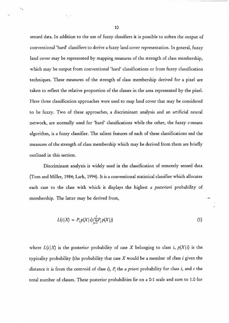
Discriminant analysis is widely used in the classification of remotely sensed data

(Tom and Miller, 1984; Lark, 1994). It is a conventional statistical classifier which allocates

each case to the class with which it displays the highest a posteriori probability of

membership. The latter may be derived from,

L(z IX) = Pi p(xl i)/k p(xli) (1)

where L(i (X) is the posterior probability of case X belonging to class i, p(Xli) is the

typicality probability (the probability that case X would be a member of class i given the

distance it is from the centroid of class t), P, the a priori probability for class i, and c the

total number of classes. These posterior probabilities lie on a 0-1 scale and sum to 1.0 for

11

each pixel. Further details on the algorithm used are given in Klecka (1980).

Problems, especially in relation to distribution assumptions, with statistical classifiers

such as discriminant analysis have led to increased use of alternative approaches. One

particularly attractive alternative for the supervised classification of remotely sensed data

is the use of artificial neural networks. An artificial neural network is constructed from a

set of simple processing units interconnected by weighted channels according to some

architecture (Aleksander and Morton, 1990; Fischer and Gopal, 1993). Typically a layered

architecture is used for classification (Figure 1). In this type of network each unit in a layer

is connected to every unit in the next layer. The data are entered at the input layer, pass

through one or more hidden layers to the output layer. The latter comprises one unit for

each class in the classification and is where class allocation may be determined.

Each unit in the network consists of a number of input channels, an activation

function and an output channel. Signals impinging on a unit's inputs are multiplied by the

inter-connecting channel's weight and are summed to derive the unit's net input. Thus for

the unit s the net input may be determined from,

nets = Ea,w, (2)

where a, is the magnitude of the rth input and qv, the weight of the interconnection

channel. This net input (nets) is then transformed by the activation function to produce an

output for the unit (Schalkoff, 1992). Typically a sigmoid activation function such as,

1 os = 1 + exp

nets (3)

where X is a gain parameter is used. The output of a network unit is sometimes referred

12

to as its activation level. The magnitude of the activation level of a unit in the output layer

is a measure of the strength of membership to the class associated with the unit. A 'hard'

classification is achieved by allocating each pixel to the class associated with the unit in the

output layer with the highest activation level.

Classification with an artificial neural network usually begins with the network

weights connecting the units set at random. Generally a backpropagation learning

algorithm (Rumelhart et al., 1986) is used to train the network to correctly characterise the

classes. Network training begins with the input of the training data from which an output

may be computed. Since the desired output is known for the training data the error in the

computed output may be determined. This is then fed backward through the network to

the input layer with the weights connecting units changed in proportion to the calculated

error (Aleksander and Morton, 1990; Schalkoff, 1992). The training data are then entered

again and the process repeated. Thus with backpropagation learning the aim is to iteratively

minimize an error function over the network outputs and a set of target outputs, taken

from a training data set. The process continues until the error value converges to a

(possibly local) minima. Conventionally the error function is given as,

E = - 0)2 (4)

where Ti is the target output vector for the training set T) and 0, is the output

vector from the network for the given training set. On each iteration backpropagation

recursively computes the gradient or change in error with respect to each weight (dE/dw)

in the network and these values are used to modify the weights between network units.

The weight change on the eh iteration is achieved by,

13

Ow, = -n(dE/dw), + (5)

where n and a are parameters which define the learning rate and momentum which

facilitate network learning (Schalkoff, 1992). Once trained the network may be used for the

classification of cases of unknown class membership.

The fuzzy c-means clustering algorithm may be used to subdivide a data set into c

clusters or classes. It is a non-hierarchical clustering technique. It begins by randomly

assigning cases (pixels) to classes and then, iteratively, moves cases to other classes with the

aim of minimizing the generalised least-squared error,

n c

im(U,v) = E E (tiJm II Yivill2 (6) k - 1 1-.1 A

where U is a fuzzy c-partition of the data set Y containing n cases (y„ y2,.., y,,), c is the

number of classes, II Li is an inner product norm, v is a vector of cluster centres, v, is the

centre of cluster i, and in is a weighting component that lies within the range 1:5 771...c. co

which determines the degree of fuzziness. The squared distance between yk and v, is derived

from,

II yk-vi II 2 = FIT A (yk-v)

(7) A

-1 A number of norms may be selected. Here the Mahalanobis norm, A = Cy, was used, where

Cy is the covariance matrix of the data set Y. The elements of U, uik , represent the grade

of membership of a case to a class. These membership values satisfy the constraints,

14

UtkE X0,1] (8a)

ht ik> 0, i=1...c (8b)

Euik = 1, k= 1...n (8c) i-1

In a fuzzy c-partition of a data set membership functions characterise the

membership of each case in all classes. These memberships lie on a 0-1 scale and the

memberships for each case sum to unity. These membership values indicate the degree of

similarity between a case and a class. Memberships close to unity indicate a high degree of

similarity between a case and a class whereas memberships close to zero indicate little

similarity between a case and a class. Further details and examples of the use of this

algorithm may be found in the literature such as Cannon et al. (1986), Fisher and Pathirana

(1990) and Key et al. (1989) and a listing of the fuzzy c-means clustering (unsupervised)

algorithm may be found in Bezdek et al. (1984). Since the classes are known a priori in a

supervised classification the fuzzy c-means clustering algorithm may be modified so that the

classification is based on class centres provided by the analyst from training samples (Key

et al., 1989).

In performing a classification with the fuzzy c-means algorithm the analyst must

select the value of the weighting component m. When in =1 a 'hard' or conventional

classification may be obtained in which each pixel is associated unequivocally with just one

class. There is no optimal value of m and most studies have used a value in the range

1.5 < m < 3.0 (Bezdek et al., 1984; McBratney and Moore, 1985). To aid the selection an

appropriate value of in and describe the quality of the land cover representation derived

from an analysis a measure of classification accuracy is required.

15

The posterior probabilities, output unit activation levels and fuzzy membership

values derived from the discriminant analysis, artificial neural network and fuzzy c-means

classifications respectively are all measures of the strength of class membership that may

be mapped to represent fuzzy land cover. The use of each measure for the representation

of fuzzy land cover is outlined below in section 6. First the procedures for the evaluation

of the accuracy of the land cover representation provided by a classification will be

discussed.

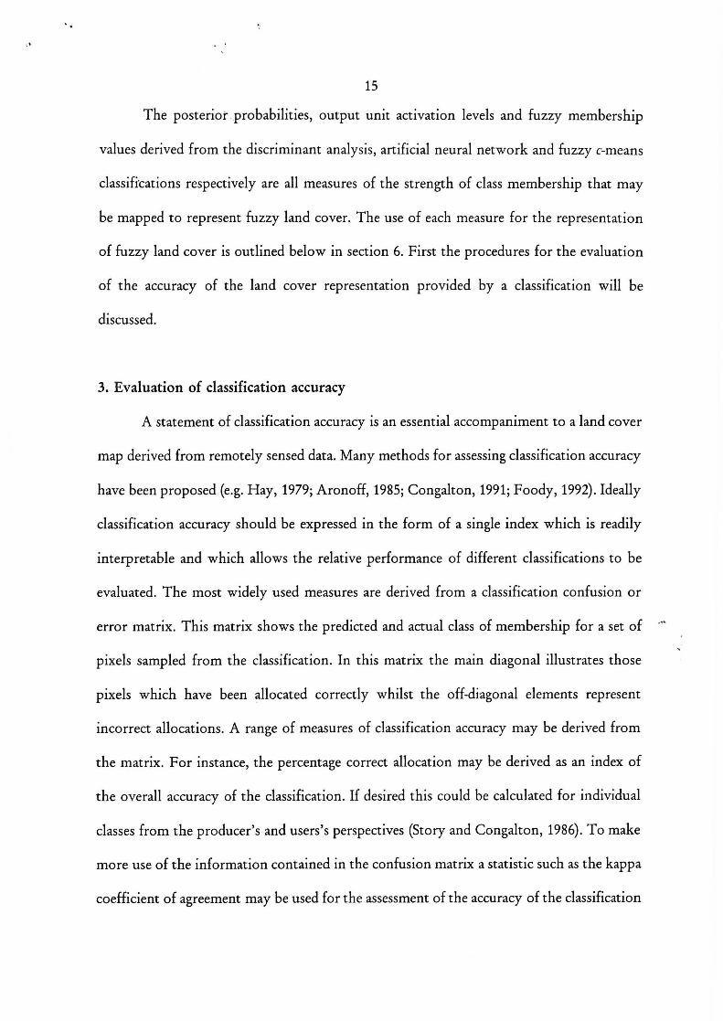
3. Evaluation of classification accuracy

A statement of classification accuracy is an essential accompaniment to a land cover

map derived from remotely sensed data. Many methods for assessing classification accuracy

have been proposed (e.g. Hay, 1979; Aronoff, 1985; Congalton, 1991; Foody, 1992). Ideally

classification accuracy should be expressed in the form of a single index which is readily

interpretable and which allows the relative performance of different classifications to be

evaluated. The most widely used measures are derived from a classification confusion or

error matrix. This matrix shows the predicted and actual class of membership for a set of

pixels sampled from the classification. In this matrix the main diagonal illustrates those

pixels which have been allocated correctly whilst the off-diagonal elements represent

incorrect allocations. A range of measures of classification accuracy may be derived from

the matrix. For instance, the percentage correct allocation may be derived as an index of

the overall accuracy of the classification. If desired this could be calculated for individual

classes from the producer's and users's perspectives (Story and Congalton, 1986). To make

more use of the information contained in the confusion matrix a statistic such as the kappa

coefficient of agreement may be used for the assessment of the accuracy of the classification

16

as a whole and for individual classes after making some compensation for chance agreement

(Cohen, 1960; Congalton, 1991).

One fundamental problem with the use of accuracy measures derived from the

classification confusion matrix is that they are only appropriate for use with a 'hard'

classification. Thus these measures of classification accuracy may be derived when each

pixel is associated with only one class in the classification and only one class in the ground

data (Congalton et al., 1983; Gong and Howarth, 1990). Consequently, an allocation is

either correct or incorrect. Although account may be made for factors such as varying

degrees of severity of error (Cohen, 1968), the measures of classification accuracy derived

from the confusion matrix are inappropriate for the evaluation of fuzzy classifications. In

some investigations a fuzzy classification has been produced but in order to evaluate the

accuracy of the classification it has been necessary to 'harden' the classification output

and/or focus only on pure pixels in the data set to enable a conventional measure of

classification accuracy to be calculated (e.g. Foody and Trodd, 1993). The resulting accuracy

statement is not, however, a good measure of the accuracy of a fuzzy classification.

Furthermore, as the pixel is generally the spatial unit used in accuracy assessment and as

the majority of image pixels may be mixed (Crapper, 1984), multiple and partial class

membership may therefore be considered to be a function of both the remotely sensed and

ground data sets. The ground data used also are often not error-free (Curran and

Williamson, 1985; Curran and Hay, 1986; Bauer et al., 1994) and may be based on

subjective assessments which can be a source of ambiguity and confusion within them.

There may therefore also be occasions when the ground data are fuzzy or where there is

ambiguity in the ground data (Gopal and Woodcock, 1994). Again it may be possible to

'harden' these data to enable the accuracy to be assessed by a conventional measure derived

17

from a confusion matrix but the end result is not an evaluation of the fuzzy classification.

There is therefore a need to derive measures of classification accuracy which go

beyond the confusion matrix (Congalton, 1994). A number of approaches have been

suggested with emphasis on fuzzy measures. Gopal and Woodcock (1994), for instance,

show how a number of fuzzy sets techniques may be used to derive a range of indicators

of classification performance. The methods used, however, are only appropriate for the

situation in which there is ambiguity in the ground data but not the classification output

(i.e., the ground data are fuzzy and the classification is 'hard'). Furthermore, the methods

do not allow the comparison of classifications, which is relatively easy with conventional

measures such as the kappa coefficient (Cohen, 1960). Other approaches that have been

used are based on measures of entropy (e.g. Finn, 1993; Maselli et al., 1994; Foody, 1995a).

Entropy is a measure of uncertainty and information formulated in terms of probability

theory, which expresses the relative support associated with mutually exclusive alternative

classes (Klir and Folger, 1988). When two or more alternative classes have non-zero

probabilities associated with them then each probability is in conflict with the others.

When there is a finite set of alternative classes the expected value of conflict is given by the

Shannon entropy (Klir, 1994). This may be used to describe the variations in class

membership probabilities associated with each pixel. Entropy is therefore particularly

attractive as an indicator of classification quality in situations where ambiguity exists as it

indicates the degree to which the class membership probabilities are partitioned between

the defined classes. The entropy, H, of a probability distribution, p, may be calculated from

the class membership probabilities, p(x), contained through,

H(p) = -R(x)log2p(x)

(9)

18

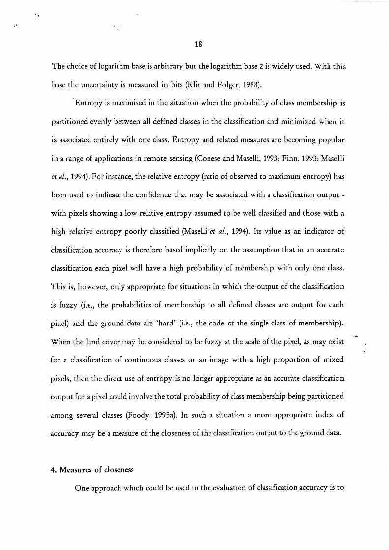
The choice of logarithm base is arbitrary but the logarithm. base 2 is widely used. With this

base the uncertainty is measured in bits (Klir and Folger, 1988).

Entropy is maximised in the situation when the probability of class membership is

partitioned evenly between all defined classes in the classification and minimized when it

is associated entirely with one class. Entropy and related measures are becoming popular

in a range of applications in remote sensing (Conese and Maselli, 1993; Finn, 1993; Maselli

et al., 1994). For instance, the relative entropy (ratio of observed to maximum entropy) has

been used to indicate the confidence that may be associated with a classification output -

with pixels showing a low relative entropy assumed to be well classified and those with a

high relative entropy poorly classified (Maselli et al., 1994). Its value as an indicator of

classification accuracy is therefore based implicitly on the assumption that in an accurate

classification each pixel will have a high probability of membership with only one class.

This is, however, only appropriate for situations in which the output of the classification

is fuzzy (i.e., the probabilities of membership to all defined classes are output for each

pixel) and the ground data are 'hard' (i.e., the code of the single class of membership).

When the land cover may be considered to be fuzzy at the scale of the pixel, as may exist

for a classification of continuous classes or an image with a high proportion of mixed

pixels, then the direct use of entropy is no longer appropriate as an accurate classification

output for a pixel could involve the total probability of class membership being partitioned

among several classes (Foody, 1995a). In such a situation a more appropriate index of

accuracy may be a measure of the closeness of the classification output to the ground data.

4. Measures of closeness

One approach which could be used in the evaluation of classification accuracy is to

19

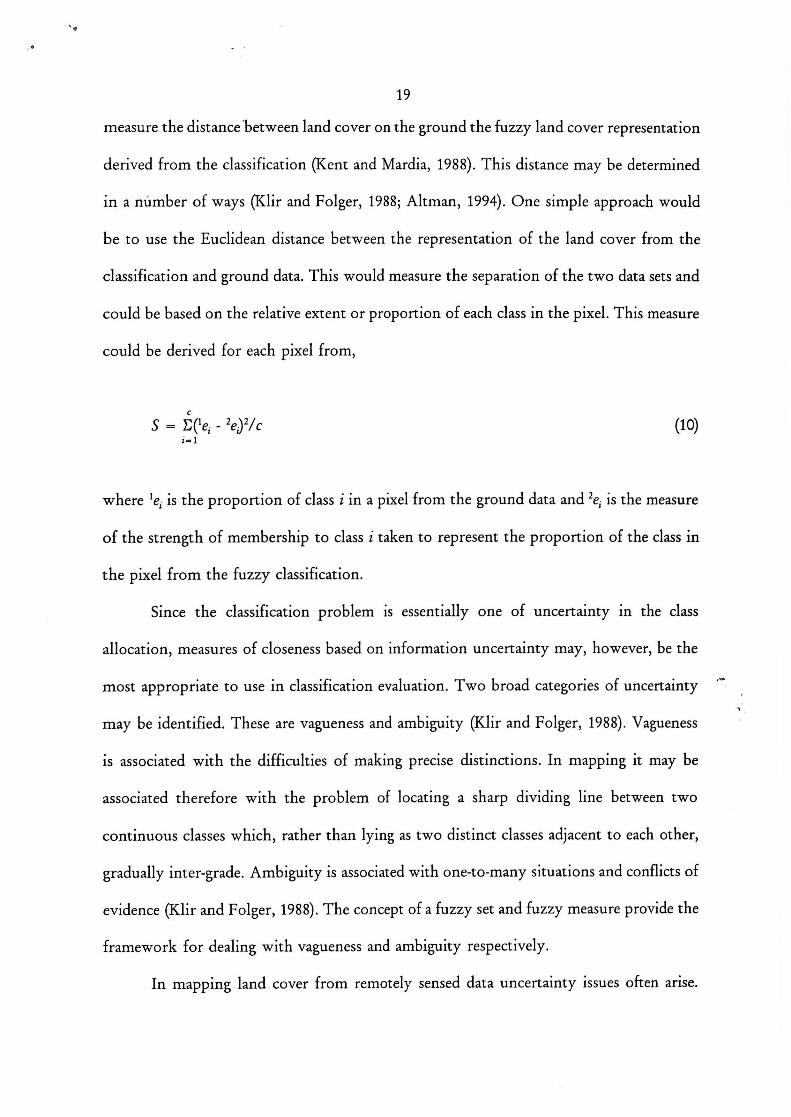
measure the distancebetween land cover on the ground the fuzzy land cover representation

derived from the classification (Kent and Mardia, 1988). This distance may be determined

in a number of ways (Klir and Folger, 1988; Altman, 1994). One simple approach would

be to use the Euclidean distance between the representation of the land cover from the

classification and ground data. This would measure the separation of the two data sets and

could be based on the relative extent or proportion of each class in the pixel. This measure

could be derived for each pixel from,

S = E(1et - 262/c (10)

where let is the proportion of class i in a pixel from the ground data and 2e, is the measure

of the strength of membership to class i taken to represent the proportion of the class in

the pixel from the fuzzy classification.

Since the classification problem is essentially one of uncertainty in the class

allocation, measures of closeness based on information uncertainty may, however, be the

most appropriate to use in classification evaluation. Two broad categories of uncertainty

may be identified. These are vagueness and ambiguity (Klir and Folger, 1988). Vagueness

is associated with the difficulties of making precise distinctions. In mapping it may be

associated therefore with the problem of locating a sharp dividing line between two

continuous classes which, rather than lying as two distinct classes adjacent to each other,

gradually inter-grade. Ambiguity is associated with one-to-many situations and conflicts of

evidence (Klir and Folger, 1988). The concept of a fuzzy set and fuzzy measure provide the

framework for dealing with vagueness and ambiguity respectively.

In mapping land cover from remotely sensed data uncertainty issues often arise.

20

Uncertainty may be quantified in a number of ways (Klir and Folger, 1988; Pal and

Bezdek, 1994). In probabilistic systems entropy has been used successfully to illustrate the

accuracy of a classification (Maselli et al., 1994; Foody, 1995a). However, it was noted

above that entropy may not be a good indicator of classification quality if multiple and

partial class membership is a feature of both the classification output and ground data.

However, since there is ambiguity in both the fuzzy classification and ground data the

entropy of each may be calculated. It is then possible to assess the closeness of the two

probability distributions for each pixel, derived from the fuzzy classification output and

the fuzzy ground data. One approach could be to assess the similarity of the land cover

representation provided by the classification output to the ground data through an

evaluation of their mutual information content (Conese and Maselli, 1993; Finn, 1993).

Alternatively the distance between the two data sets could be assessed. Essentially the aim

is to express the information closeness of a pair of probability distributions, 'p and 2p. In

the evaluation of the accuracy of a fuzzy land cover map the probability distribution of the

ground data ('p) and that of the fuzzy classification output (2p) for a pixel would be used.

An approach which may be used is to calculate the directed divergence or cross-entropy.

Directed divergence may be derived from,

d('r), 2p) = - 1p(x)log2p(x) + 1p(x)log, tp(x) (11)

This provides a measure of the closeness of the classification to the ground data. A small

difference would, for instance, indicate that the classification was an accurate representation

of the land cover (Foody, 1995a). This measure may be used as a criterion to evaluate the

degree of similarity between two data sets (Chang et al., 1994). Directed divergence,

21

however, may only be derived when the supports of the probability distributions to be

compared are compatible. Specifically the support 1p g support 2p. Higashi and Klir

(1983); however, present a measure of information closeness which is applicable to any pair

of probability distributions. This generalised measure of information closeness, D, may be

derived from,

D('p, 2p) = d('p, 1 P +2 213 ) + d(2 p, 113 2 2P )

,,(x) 2F.„(x )

= 1/)(x)log,V,(x) - Fp(x)log, 1f" 2

iiy Ex2P(01°g22P(X) 273(x)10g2 if" 2

2.„ F"y

(12)

and used to assess the closeness of pairs of probability distributions.

The measures S and D should enable the closeness of the fuzzy land cover

representation, derived from the three classification techniques, to the fuzzy ground data

to be assessed. Both S and D are used here to evaluate the accuracy of a set of fuzzy

classifications derived from remotely sensed data, although D was developed for use with

probability distributions.

5. Test sites and data

The test site was a 0.5 km2 area located adjacent to the University campus on the

fringe of the City of Swansea, UK. Airborne thematic mapper (ATM) data in eleven

spectral wavebands were acquired for the site with a Daedalus 1268 sensor with a spatial

resolution of approximately 1.5m in 1990. The advantage of using fine spatial resolution

data for a small test site was that the composition of image pixels could be evaluated

accurately.

22

This test-site was comprised of mainly three land cover classes, trees, grass and

asphalt (car park), and these could be readily identified from the imagery. For the purpose

of this investigation each pixel in this fine spatial resolution image was assumed to be pure

and classified visually into the three classes. This classification was verified in the field and

used as ground/reference data on the distribution of the three land cover classes. To

simplify the analysis of this data set, only the data from three wavebands, which account

for much of the dimensionality and information content of ATM data (Townshend, 1984),

were used. These were the data in the 605-625nm, 695-750nm and 1550-1750nm wavebands.

The ATM data were then spatially degraded with an 11x11 low pass (mean) filter to

simulate an image with a relatively coarse spatial resolution; further details on these data

and the test site may be found in Foody and Cox (1994). For each pixel in this simulated

coarse spatial resolution image the proportion of three land cover classes contained within

it could be derived from the classification of the spatially undegraded image. Using 5 pure

pixels of each class as training sites the simulated coarse spatial resolution image was then

classified into the three classes by the discriminant analysis, artificial neural network and

fuzzy c-means algorithm. To vary the degree of fuzziness in the land cover representations

derived from the fuzzy c-means algorithm the analysis was repeated with different values

for the weighting parameter m. In addition to the conventional 'hard' classification outputs

the posterior probabilities of class membership from the discriminant analysis, output unit

activation levels from the artificial neural network and fuzzy memberships generated from

the analyses with the fuzzy c-means algorithm were output for each pixel. The accuracy

of the classification outputs derived were assessed relative to ground data on class

membership for a sample of 35 pixels. Although this is a relatively small sample it is large

enough to illustrate the methods. The ground data for each pixel comprised the proportion

23

of each land cover class in the 35 pixels sampled from the simulated coarse spatial

resolution image. These lie on a 0-1 scale and sum to unity for each pixel. Although not

strictly probabilities they may reasonably be considered as such and forming a probability

distribution for each pixel.

Thus the data for each pixel used to evaluate the accuracy of the land cover

representations derived from the fuzzy classifications comprised the strength of membership

to all classes derived from the three classification techniques together with ground data in

the form of the proportion of each class in the area represented by the pixel. The closeness

of each fuzzy land cover representation derived to the ground data was assessed by

correlation analysis as well as with measures S and D.

6. Results and discussion

The discriminant analysis was used to produce a conventional statistical classification

of the data. The mean entropy of the 35 testing pixels was 0.095 with a corresponding

mean relative entropy of 0.059. These values could be interpreted as indicating a fairly

good classification. However, as the entropy value was greater than the minimum value this

indicated the posterior probability of class membership for all pixels was not associated

solely with a single class. This is desirable for a fuzzy classification. However, the posterior

probabilities of class membership output from the analysis were generally either high or

low with little variation between these extremes. Thus although the magnitude of

probabilities did to some extent reflect the composition of the pixels the relationships were

not strong (Figure 2). Relative to the 'hard' classification output, however, the land cover

representation portrayed by the probabilities was closer, as measured by both S and D, to

the ground data (Table 1). These results show two main features. Firstly, they reinforce the

24

danger of using entropy as a measure of classification accuracy when mixed pixels are

present and secondly, that a conventional 'hard' statistical classification may be softened

to provide a more appropriate representation of fuzzy land cover than the 'hard'

classification.

Although both S and D may be derived for the probabilities output from the

discriminant analysis the use of D at first seems inappropriate for the evaluation of the

accuracy of the non-probabilistic fuzzy land cover representations based on fuzzy

memberships and the activation level of artificial neural network output units. Although

similar in some ways to posterior probabilities of class membership, fuzzy membership

values and artificial neural network output unit activation levels are not probabilities and

should not be treated as such (Bezdek, 1993). One obvious difference is that fuzzy

memberships, in general, and the activation level of artificial neural network output units

need not sum to 1.0 for each pixel. However, because of the constraints (8) in the fuzzy

c-means algorithm the vector of fuzzy memberships for each pixel is mathematically

identical to a probability vector enabling a complete formal analogy to Shannon's entropy

for a fuzzy c-partition (Bezdek, 1981). With the artificial neural network, the output unit

activation levels were on a scale 0-1 but need not sum to 1.0 for a pixel. Moreover, the

sigmoid transfer function of the output units imposed a bias toward high or low values

which results in a non-linear relationship between the activation level of a class and the

proportion of the pixel composed of that class. Since the nature of the transfer function

was known (equation 3) its effect was removed, which resulted in activation levels which

should be more linearly related to the proportion cover of a class (Foody, 1995b). These

transfer-function corrected activation levels were then rescaled and normalised so that they

lay on a C-1 scale sum to 1.0 for each pixel and only these rescaled activation levels were

25

used in the research. Although neither these rescaled activation levels or fuzzy memberships

are probabilities both are mathematically similar and, for comparative purposes, were used

in the 'calculation of the distance measure D. The closeness of all the classification outputs

to the ground data were also assessed with the generally applicable distance measure S.

As with the discriminant analysis the artificial neural network was used to derive

a 'hard' classification of the data. The artificial neural network used was a four-layered

feedforward network with three input units, twelve hidden units arranged in two equally

sized hidden layers and three output units (Figure 1); the number of input and output units

was determined by the number of discriminating variables and classes respectively. The

number of hidden units is generally determined subjectively. Here the number of hidden

units was selected after a series of trial runs and with the aim of ensuring both a high

learning and generalisation capacity. Each unit had a sigmoid activation function and an

external bias unit. A stochastic backpropagation learning algorithm was used with X= 1.0

and the parameters n and a were set at 0.1 and 0.9 respectively. Training the artificial

neural network involved 2000 iterations, by the end of which the average root sum squared

error was 0.000521.

The rescaled activation level of the units in the output layer were derived for each

of the 35 testing pixels. As with the probabilities of class membership derived from the

discriminant analysis these were then related to the ground data (Figure 3). The activation

level of an output unit was found to be strongly related to the proportion of the pixel area

covered by the class associated with that unit. This indicated that although artificial neural

networks have generally been used to drive a 'hard' classification the activation levels of

the output units may, as measures of the strength of class membership, be mapped to

provide a softened representation of land cover. The closeness of this representation to the

26

ground data was assessed with both S and D. The results showed that the softened network

classification output provided a more accurate representation of the fuzzy land cover than

the 'hard' classification. Moreover, the softened artificial neural network classification was

more accurate than the softened classification from the discriminant analysis (Table 1) with

a strong relationship between the output unit activation level and the proportion of the

pixel area covered by the class associated with the unit (Figure 3).

Four fuzzy classifications with the fuzzy c-means algorithm were performed with

different values for the weighting parameter m. These were a fairly 'hard' analysis with

m =1.2 and three fuzzier classifications with m=1.5, 2.0 and 2.5. From each classification

the fuzzy membership values for each pixel to each class were output. For completeness

the end points of the continuum of fuzzy classifications were also simulated and their

closeness to the ground data assessed. The 'hard' classification, equivalent to m =1.0, had

been derived by allocating each pixel to the class with which it had highest membership

value in the analysis with m =1.2. The fuzziest classification output would be derived with

m = co in which class membership would be partitioned evenly between the classes. This

was therefore simulated by dividing the total membership for each pixel equally between

the classes. Combined with the reference data on the land cover composition of each pixel

this enabled an assessment of the accuracy of the fuzzy land cover representations derived

from the fuzzy c-means classifications.

With the weighting parameter m=1.2 the fuzzy membership values derived tended

towards 1.0 and 0.0, characteristic of a fairly 'hard' classification (Figure 4). These fuzzy

memberships were relatively poorly related to the land cover class composition of the

pixels, with the relationship between the membership values and coverage of a class having

some similarity to the results from the discriminant analysis (Figure 2). The membership

27

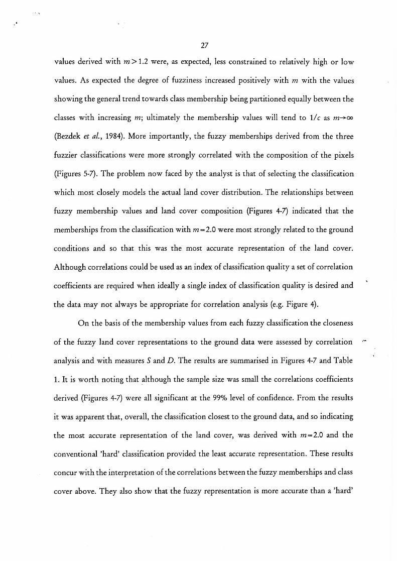
values derived with m > 1.2 were, as expected, less constrained to relatively high or low

values. As expected the degree of fuzziness increased positively with m with the values

showing the general trend towards class membership being partitioned equally between the

classes with increasing m; ultimately the membership values will tend to 1/c as m—>oo

(Bezdek et aL, 1984). More importantly, the fuzzy memberships derived from the three

fuzzier classifications were more strongly correlated with the composition of the pixels

(Figures 5-7). The problem now faced by the analyst is that of selecting the classification

which most closely models the actual land cover distribution. The relationships between

fuzzy membership values and land cover composition (Figures 4-7) indicated that the

memberships from the classification with m=2.0 were most strongly related to the ground

conditions and so that this was the most accurate representation of the land cover.

Although correlations could be used as an index of classification quality a set of correlation

coefficients are required when ideally a single index of classification quality is desired and

the data may not always be appropriate for correlation analysis (e.g. Figure 4).

On the basis of the membership values from each fuzzy classification the closeness

of the fuzzy land cover representations to the ground data were assessed by correlation --

analysis and with measures S and D. The results are summarised in Figures 4-7 and Table

1. It is worth noting that although the sample size was small the correlations coefficients

derived (Figures 4-7) were all significant at the 99% level of confidence. From the results

it was apparent that, overall, the classification closest to the ground data, and so indicating

the most accurate representation of the land cover, was derived with m=2.0 and the

conventional 'hard' classification provided the least accurate representation. These results

concur with the interpretation of the correlations between the fuzzy memberships and class

cover above. They also show that the fuzzy representation is more accurate than a 'hard'

28

one and allow the selection of the most appropriate representation.

Interpretation of the measures S and D, however, requires information on the

sample used in its definition. Although the fuzzy classification derived from the fuzzy c-

means algorithm with m = 2.0 appeared to be the closest of all the classifications produced

to the ground data the results were more variable on a per-pixel basis. This is illustrated

in Table 2 which summarises the results for a pure pixel and one of mixed land cover

composition. Note how the 'hard' classifications generally provided the most accurate

representation of the pure pixel and the closeness of the fuzzy representations derived from

the classifications based on the fuzzy c-means algorithm to the ground data declined as m

increased. Conversely, for the mixed pixel the 'hard' representations were generally furthest

from ground data and, for this pixel, the closest representation derived with the fuzzy c-

means algorithm was derived with m= cc, a consequence of its area being split fairly evenly

between the three classes. Therefore if S and D are to be used as indicators of overall

classification accuracy the testing sample of pixels acquired to assess classification accuracy

should be drawn from a random sample. Information on the sampling design used in the

acquisition of testing cases should therefore be included in accuracy statements (Janssen and

van der Wel, 1994) to help their correct interpretation.

7. Summary and conclusions

Land cover is generally mapped from remotely sensed data through the application

of a conventional 'hard' classification technique. In the output of this type of classification

each pixel is associated unambiguously with a single class. Recognition that pixels in an

image may have multiple and partial class membership, however, severely limits the

appropriateness of such approaches to land cover mapping. Since the majority of pixels in

29

an image may have a mixed land cover composition there is therefore a need for conceptual

and methodological change in mapping land cover from remotely sensed data.

Fuzzy classification approaches may, however, enable a more accurate and realistic

representation of land cover than conventional 'hard' classification techniques. A fuzzy

classification output may be derived by softening the output of a 'hard' classifier or

through the use of a fuzzy classifier. Although fuzzy classifications appear to provide a

more appropriate representation of land cover a major limitation to their use and

interpretation is the evaluation of the accuracy of the land cover representation derived

(Goodchild, 1994) . The measures of accuracy usually used in the evaluation of a

classification were derived for application to 'hard' classification outputs in which cases are

associated unambiguously with one class. Such measures are inappropriate for the

evaluation of a classification in which multiple and partial class membership is a feature.

Measures which show how the strength of class membership in the classification output is

partitioned between the classes, such as entropy, are also inappropriate as the fuzziness of

the land cover on the ground is overlooked. An approach is therefore required which

accommodates for the fuzziness in both the classification output and the ground data

against which the accuracy of the representation is assessed. This may be achieved by

measuring the closeness of the land cover composition in the fuzzy classification, as

reflected by the strengths of class membership, to the composition measured on the

ground. This may be achieved with the use of a simple measures of distance such as the

euclidean distance (measure S) or through the use of a measure of information closeness for

probability distributions (measure D) . These two measures were used to assess the accuracy

of fuzzy classifications derived from three classification approaches. Two of these, a

discriminant analysis and an artificial neural network, are usually used to derive 'hard'

30

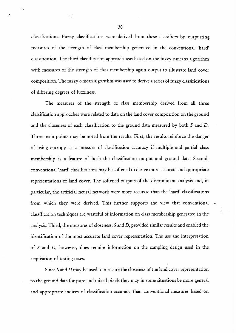
classifications. Fuzzy classifications were derived from these classifiers by outputting

measures of the strength of class membership generated in the conventional 'hard'

classification. The third classification approach was based on the fuzzy c-means algorithm

with measures of the strength of class membership again output to illustrate land cover

composition. The fuzzy c-mean algorithm was used to derive a series of fuzzy classifications

of differing degrees of fuzziness.

The measures of the strength of class membership derived from all three

classification approaches were related to data on the land cover composition on the ground

and the closeness of each classification to the ground data measured by both S and D.

Three main points may be noted from the results. First, the results reinforce the danger

of using entropy as a measure of classification accuracy if multiple and partial class

membership is a feature of both the classification output and ground data. Second,

conventional 'hard' classifications may be softened to derive more accurate and appropriate

representations of land cover. The softened outputs of the discriminant analysis and, in

particular, the artificial neural network were more accurate than the 'hard' classifications

from which they were derived. This further supports the view that conventional

classification techniques are wasteful of information on class membership generated in the

analysis. Third, the measures of closeness, S and D, provided similar results and enabled the

identification of the most accurate land cover representation. The use and interpretation

of S and D, however, does require information on the sampling design used in the

acquisition of testing cases.

Since S and D may be used to measure the closeness of the land cover representation

to the ground data for pure and mixed pixels they may in some situations be more general

and appropriate indices of classification accuracy than conventional measures based on

31

classification confusion matrices. Before they could be adopted, research on their properties,

especially in terms of identifying significant differences between classification outputs would

be required. None-the-less these measures do enable the assessment of the accuracy of fuzzy

classifications and this should help further develop the use of fuzzy land cover mapping

approaches. Given the significance of the mixed pixel problem the recognition and

accommodation of fuzziness in the classification output and assessment of accuracy should

provide later users of the land cover classification derived with more appropriate and useful

information. Further advances may be made when fuzziness is accommodated in the

training stage in addition to the class allocation and testing stages of the supervised

classification.

Acknowledgements

I am grateful to the NERC for provision of the ATM data as part of the its 1990 airborne

campaign. The neural network was constructed with the NCS NeuralDesk package.

References

Aleksander, I., and Morton, H., 1990, An Introduction to Neural Computing, (Chapman and

Hall, London).

Altman, D., 1994, Fuzzy set theoretic approaches for handling imprecision in spatial

analysis. International Journal of Geographical Information Systems, 8, 271-289.

Aronoff, S., 1985, The minimum accuracy value as an index of classification accuracy.

Photogrammetric Engineering and Remote Sensing, 51, 593-600.

32

Atkinson, P. M., 1995, Scale and spatial dependence. In Scaling-up, edited by P. R. van

Gardingen, G. M. Foody and P. J. Curran (Cambridge University Press,

Cambridge) (in press).

Bauer, M. E., Burk, T. E., Ek, A. R., Coppin, P. R., Lime, S. D., Walsh, T. A., and

Walters, D. K., 1994, Satellite inventory of Minnesota forest resources.


Benediktsson, J. A., Swain, P. H., and Ersoy, 0. K., 1990, Neural network approaches

versus statistical methods in classification of multisource remote sensing data. IEEE

Transactions on Geoscience and Remote Sensing, 28, 540-551.

Bezdek, J. C., 1981, Pattern Recognition with Fuzzy Objective Functions, (Plenum Press, New

York).

Bezdek, J. C., Ehrlich, R., and Full, W., 1984, FCM: the fuzzy c-means clustering

algorithm, Computers and Geosciences, 10, 191-203.

Bezdek, J. C., 1993, Fuzzy models - what are they, and why? IEEE Transactions on Fuzzy

Systems, 1, 1-6.

Bosserman, R. W., and Ragade, R. K., 1982, Ecosystem analysis using fuzzy set theory.

Ecological Modelling, 16, 191-208.

Campbell, J. B., 1987, Introduction to Remote Sensing, (Guilford Press, New York).

Cannon, R. L., Dave, J. V., Bezdek, J. C., and Trivedi, M. M., 1986, Segmentation of a

thematic mapper image using the fuzzy c-means clustering algorithm. IEEE


Chang, C-I., Chen, K., Wang, J., and Althouse, M. L. G., 1994, A relative entropy-based

approach to image thresholding. Pattern Recognition, 27, 1275-1289.

Cohen, J., 1960, A coefficient of agreement for nominal scales. Educational and

33

Psychological Measurement, 20, 37-46.

Cohen, J., 1968, Weighted kappa. Psychological Bulletin, 70, 213-220.

Conese, C., and Maselli, F., 1993, Selection of optimum bands from TM scenes through

mutual information analysis. ISPRS Journal of Photogrammetry and Remote Sensing,

48 (3), 2-11.

Congalton, R. G., 1991, A review of assessing the accuracy of classifications of

remotely sensed data. Remote Sensing of Environment, 37, 35-46.

Congalton, R. G., 1994, Accuracy assessment of remotely sensed data: future needs and

directions. Pecora 12: Land Information from Space-Based Systems, (American Society

for Photogrammetry and Remote Sensing, Bethesda), pp. 385-388.

Congalton, R. G., Oderwald, R. G., and Mead, R. A., 1983, Assessing Landsat classification

accuracy using discrete multivariate analysis statistical techniques, Photogrammetric

Engineering and Remote Sensing, 49, 1671-1678.

Corves, C., and Place, C. J., 1994, Mapping the reliability of satellite-derived landcover

maps - an example from central Brazilian Amazon Basin. International Journal of

Remote Sensing, 15, 1283-1294.

Crapper, P. F., 1984, An estimate of the number of boundary cells in a mapped landscape

coded to grid cells. Photogrammetric Engineering and Remote Sensing, 50, 1497-1503.

Curran, P. J., and Hay, A. M., 1986, The importance of measurement error for certain

procedures in remote sensing at optical wavelengths. Photogrammetric Engineering

and Remote Sensing, 52, 229-241.

Curran, P. J., and Williamson, H. D., 1985, The accuracy of ground data used in remote

sensing investigations. International Journal of Remote Sensing, 6, 1637-1651.

DeFries, R. S., and Townshend, J. R. G., 1994, Global land cover: comparison of ground-

34

based data sets to classifications with AVHRR data. In Environmental Remote

Sensing from Regional to Global Scales, edited by G. M. Foody and P. J. Curran

(Wiley, Chichester), pp. 84-110.

Estes, J. E., and Mooneyhan, D. W., 1994, Of maps and myths. Photogrammetric


Finn, J. T., 1993, Use of the average mutual information index in evaluating classification

error and consistency. International Journal of Geographical Information Systems, 7,

349-366.

Fischer, M. M., and Gopal, S., 1993, Neurocomputing - a new paradigm for geographic

information processing. Environment and Planning A, 23, 757-760.

Fisher, P. F., and Pathirana, S., 1990, The evaluation of fuzzy membership of land cover

classes in the suburban zone. Remote Sensing of Environment, 34, 121-132.

Fisher, P. F., 1995, The pixel: a snare and a delusion. In Proceedings of Environmental GIS

and Remote Sensing, edited by P. Pan (Remote Sensing Society, Nottingham), (in

press).

Foody, G. M., 1992, Classification accuracy assessment: some alternatives to the kappa

coefficient for nominal and ordinal level classifications. Remote Sensing from

Research to Operation, (Remote Sensing Society, Nottingham), 529-538.

Foody, G. M., 1995a, Cross-entropy for the evaluation of the accuracy of a fuzzy land

cover classification with fuzzy ground data. ISPRS Journal of Photogrammetry and

Remote Sensing, (in press).

Foody, G. M., 1995b, Fuzzy modelling of vegetation from remotely sensed imagery.

Ecological Modelling, (in press).

Foody, G. M., and Cox, D. P., 1994, Sub-pixel land cover composition estimation using

35

a linear mixture model and fuzzy membership functions. International Journal of


Foody, G. M., and Trodd, N. M., 1993, Non-classificatory analysis and representation of

heathland vegetation from remotely sensed imagery. GeoJournal, 29, 343-350.

Foody, G. M., Campbell, N. A., Trodd, N. M., and Wood, T. F., 1992, Derivation and

applications of probabilistic measures of class membership from the maximum

likelihood classification. Photogrammetric Engineering and Remote Sensing, 58, 1335-

1341.

Foody, G. M., McCulloch, M. B., and Yates, W. B., 1995, Classification of remotely sensed

data by an artificial neural network: issues related to training data characteristics.


Goodchild, M. F., 1994, Integrating GIS and remote sensing for vegetation analysis and

modelling: methodological issues. Journal of Vegetation Science, 5, 615-626.

Gong, P., and Howarth, P. J., 1990, The use of structural information for improving land-

cover classification accuracies at the rural-urban fringe. Photogrammetric Engineering

and Remote Sensing, 56, 67-73.

Gopal, S., and Woodcock, C., 1994, Theory and methods for accuracy assessment of

thematic maps using fuzzy sets. Photogrammetric Engineering and Remote Sensing,

60, 181-188.

Hall, G. B., Wang, F., and Subaryono., 1992, Comparison of Boolean and fuzzy

classification methods in land suitability analysis using a geographical information

system. Environment and Planning A, 24, 497-516.

Harris, R., 1985, Contextual classification post-processing of Landsat data using a

probabilistic relaxation model. International Journal of Remote Sensing, 6, 847-866.

36

Hay, A. M., 1979, Sampling designs to test land-use map accuracy. Photogrammetric


Higashi, M., and Klir, G. J., 1983, On the notion of distance representing information

closeness: possibility and probability distributions. International Journal of General

Systems, 9, 103-115.

Hisdal, E., 1994, Interpretative versus prescriptive fuzzy set theory. IEEE Transactions on

Fuzzy Systems, 2, 22-26.

Janssen, L. V., and van der Wel, F. J. M., 1994, Accuracy assessment of satellite derived

land-cover data: a review. Photogrammetric Engineering and Remote Sensing, 60, 419-

426.

Kanellopoulos, I., Varfis, A., Wilkinson, G. G., and Megier, J., 1992, Land-cover

discrimination in SPOT HRV imagery using an artificial neural network - a 20-class

experiment. International Journal of Remote Sensing, 13, 917-924.

Kent, J. T., and Mardia, K. V., 1988, Spatial classification using fuzzy membership models.

IEEE Transactions on Pattern Analysis and Machine Intelligence, 10, 659-671.

Key, J. R., Maslanik, J. A., and Barry, R. G., 1989, Cloud classification from satellite data

using a fuzzy sets algorithm: a polar example. International Journal of Remote

Sensing, 10, 1823-1842.

Klecka, W. R., 1980, Discriminant Analysis, (Sage, Beverly Hills, CA).

Klir, G. J., 1994, On the alleged superiority of probabilistic representation of uncertainty.

IEEE Transactions on Fuzzy Systems, 2, 27-31.

Klir, G. J., and Folger, T. A., 1988, Fuzzy Sets, Uncertainty and Information, (Prentice-Hall

International, London).

Lark, R. M., 1994, Sample size and class variability in the choice of a method of

37

discriminant analysis. International Journal of Remote Sensing, 15, 1551-1555.

Maselli, F., Conese, C., and Petkov, L., 1994, Use of probability entropy for the estimation

and graphical representation of the accuracy of maximum likelihood classifications.

ISPRS Journal of Photogrammetry and Remote Sensing, 49 (2), 13-20.

Mather, P.M., 1987, Computer Processing of Remotely-Sensed Images, (Wiley, Chichester).

McBratney, A. B., and Moore, A. W., 1985, Application of fuzzy sets to climatic

classification. Agricultural and Forest Meteorology, 35, 165-185.

Moon, W. M., 1993, On mathematical representation and integration of multiple spatial

geoscience datasets. Canadian Journal of Remote Sensing, 19, 63-67.

Pal, N. R., and Bezdek, J. C., 1994, Measuring fuzzy uncertainty. IEEE Transactions on

Fuzzy Systems, 2, 107-118.

Peddle, D. R., 1993, An empirical comparison of evidential reasoning, linear discriminant

analysis and maximum likelihood algorithms for land cover classification. Canadian

Journal of Remote Sensing, 19, 31-44.

Rhind, D., and Hudson, R., 1980, Land Use, (Methuen, London).

Rosenfield, G. H., and Fitzpatrick-Lins, K., 1986, A coefficient of agreement as a measure

of thematic classification accuracy. Photogrammetric Engineering and Remote Sensing,

52, 223-227.

Rumelhart, D. E., Hinton, G. E., and Williams, R. J., 1986, Learning internal

representation by error propagation. In Parallel Distributed Processing: Explorations

in the Microstructure of Cognition, edited by D. E. Rumelhart and J. L. McClelland

(MIT Press, Cambridge MA), pp. 318-362.

Schalkoff, R. J., 1992, Pattern Recognition: Statistical, Structural and Neural Approaches,

(Wiley, New York).

38

Srinivasan, A., and Richards, J. A., 1990, Knowledge-based techniques for multi-source

classification. International Journal of Remote Sensing, 11, 505-525.

Story,. M., and Congalton, R. G., 1986, Accuracy assessment: a user's perspective,


Thomas, I. L., Benning, V. M., and Ching, N. P., 1987, Classification of Remotely Sensed

Images, (Adam Hilger, Bristol).

Tom, C. H., and Miller, L, D., 1984, An automated land-use mapping comparison of the

Bayesian maximum likelihood and linear discriminant analysis algorithms.


Townshend, J. R. G., 1984, Agricultural land-cover discrimination using thematic mapper

spectral bands. International Journal of Remote Sensing, 6, 681-698.

Townshend, J. R. G., 1992, Land cover. International Journal of Remote Sensing, 13, 1319-

1328.

Townshend, J. R. G., and Justice, C. 0., 1981, Information extraction from remotely

sensed data: a user view. International Journal of Remote Sensing, 2, 313-329.

Townshend, J., Justice, C., Li, W., Gurney, C., and McManus, J., 1991, Global land cover

classification by remote sensing: present capabilities and future possibilities. Remote

Sensing of Environment, 35, 243-255

Wang, F., 1990a, Improving remote sensing image analysis through fuzzy information

representation. Photogrammetric Engineering and Remote Sensing, 56, 1163-1169.

Wang, F., 1990b, Fuzzy supervised classification of remote sensing images. IEEE


Wang, F., 1994, The use of artificial neural networks in a geographical information system

for agricultural land-suitability assessment. Environment and Planning A, 26, 265-

39

284.

Wang, Y., and Civco, D. L., 1992, Post-classification of misclassified pixels by evidential

. reasoning: a GIS approach for improving classification accuracy of remote sensing

data. Proceedings ISPRS Conference 1992, Washington DC, 80-86.

Wood, T. F., and Foody, G. M., 1989, Analysis and representation of vegetation continua

from Landsat Thematic Mapper data for lowland heaths. International Journal of


40

Table 1. Overall closeness of the land cover representations derived from all three

classification algorithms. The mean and median values are given since the

distributions were generally positively skewed

Classifier (measure of strength of class membership)

Measure of closeness

Mean Median Mean Median

Discriminant analysis Hard 0.0997 0.0633 0.4508 0.4112 (posterior probabilities) Softened 0.0834 0.0602 0.3848 0.3384

Neural network (output Hard 0.0904 0.0612 0.3779 0.3135 unit activation level) Softened 0.0303 0.0141 0.1710 0.1269

Fuzzy c-means (fuzzy m=1.0 0.1223 0.0689 0.5181 0.4175 membership) m =1.2 0.0632 0.0450 0.2818 0.2673

m=1.5 0.0368 0.0294 0.1667 0.1410 m=2.0 0.0253 0.0138 0.1376 0.1032 m=2.5 0.0294 0.0166 0.1672 0.1347 m= 00 0.0910 0.0651 0.3757 0.3614

N

N •1-

O O

O

O

0.00

00 0

.005

9 0.

0075

0.11

40 0.

02

81

0.22

22 M 00

O

O N s.0 O

W 0 tu

cu 0 X 4-> 4.J . 4-1 E 0

(/) o 04 S-■

-0 0 u u › $... .._. 0 ,.. (1) 7:1 0 U

O

•

0 Cti 4.-> 4--■

O V CU >4 V) • .... u E , u 0 ,.. ,.. u u ›. 0 u

•

-0 -0 •

a: al 4.) ..--1 X I) . .-I

04 4-J cl.) 0 (,) fa4 v) a) ca • I. 1.) 0 6 ,+.4

v) T...) E 4.J

•

. .

-

... $.-■ • WO

O cl) ci)

4-J i••• • .••• i•-• 4-

-

■ it .--,

ct

a) 40 td

H

42

Figure captions

Figure 1. An overview of the classification of remotely sensed data by a feedfoward artificial neural

network. The network architecture comprises one unit in the input layer for each

discriminating variable and one unit in the output layer for each class. The number of

hidden layers and units is subjectively determined, often on the basis of a set of trial runs.

Each unit in the network is connected to every unit in adjacent layers by a weighted

channel. Together the network units and weighted channel act to classify the remotely

sensed data, with each case allocated to the class associated with the unit in the output layer

with the highest activation level. The network used in the research had three input units

(one for each waveband), two hidden layers each containing six units, and three output

units (one for each class).

Figure 2. Results from the discriminant analysis. (a) the relationship between the probability of

membership to trees with the proportion of the pixel area covered by trees (r=0.774); (b)

the relationship between the probability of membership to grass with the proportion of the

pixel area covered by grass (r=0.838); (c) the relationship between the probability of

membership to asphalt with the proportion of the pixel area covered by asphalt (r= 806);

(d) histogram showing the closeness of the two representations measured by S; and (e)

histogram showing the closeness of the two representations measured by D.

Figure 3. Results from the artificial neural network. (a) the relationship between the activation level

of the output unit associated with trees with the proportion of the pixel area covered by

trees (r= 0.873); (b) the relationship between the activation level of the output unit

associated with grass with the proportion of the pixel area covered by grass (r=0.866); (c)

the relationship between the activation level of the output unit associated with asphalt with

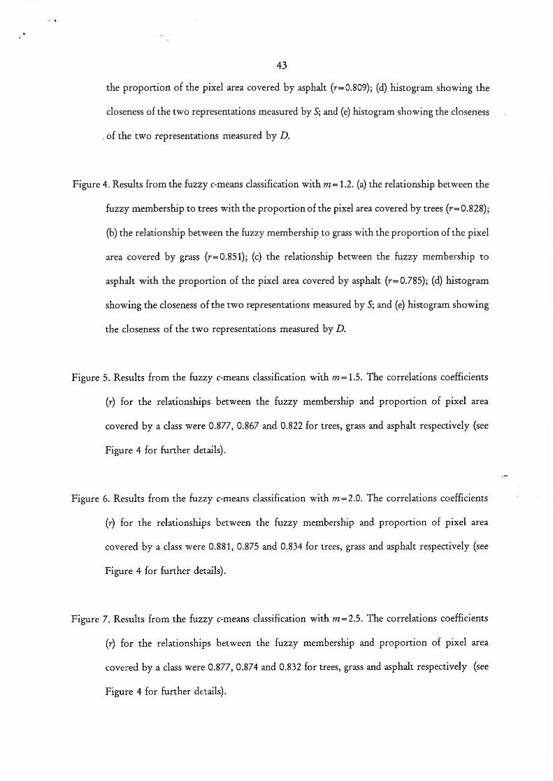
43

the proportion of the pixel area covered by asphalt (r=0.809); (d) histogram showing the

closeness of the two representations measured by S; and (e) histogram showing the closeness

of the two representations measured by D.

Figure 4. Results from the fuzzy c-means classification with m=1.2. (a) the relationship between the

fuzzy membership to trees with the proportion of the pixel area covered by trees (r= 0.828);

(b) the relationship between the fuzzy membership to grass with the proportion of the pixel

area covered by grass (r= 0.851); (c) the relationship between the fuzzy membership to

asphalt with the proportion of the pixel area covered by asphalt (r= 0.785); (d) histogram

showing the closeness of the two representations measured by S; and (e) histogram showing

the closeness of the two representations measured by D.

Figure 5. Results from the fuzzy c-means classification with m=1.5. The correlations coefficients

(r) for the relationships between the fuzzy membership and proportion of pixel area

covered by a class were 0.877, 0.867 and 0.822 for trees, grass and asphalt respectively (see

Figure 4 for further details).









Remotely sensed Artificial Neural Network discriminating variables Input

Hidden Output

Classification

-• —••

•----•=1. S.

•

• •

0.5-•

C

C

Z

C. C. --or •

( ) 00 0.2 0.4 CE 0.3 10 (b) 0.0 3.2 0.4 0.6

PropcHc!-. of trees rr of gross

00:

1.0

0.8

0.6

0.41

0.2-1

0.0 •-•-••■-•••••• S .

(c) .0 3.2 0.4 0.6 08 0

Propercr :f cs:^cf.

(d)

2•;-

, :• -

if: •

(e)

Pro b

obili

ty t

o os

pho

lt

2_

-■ •

-

o Z1.,

< o 0.2

0.0 (0) 0.0

1.0

-1

111 •

• •

• • •

•

••

•

•

• •

g

0

3

o

=

(b)

(d)

0

G,

C

0.4

0.2 i

0.0 I

•

• • •

•

•.• • • •

• •

• • •

• •

0.2 0.4 0.6 Proportion of trees

0.8 1 0.0

18

28 21 14

7

0.2

•

0.4 0.6 Propert;cn at grass

0.3 1 0

t; 8

> 0.6

2 76 0.4 , O U O< 0.21

0.0 1

•

• •

•

•

• •

•

% • • • • •

•

• •

•

S

:2: 4 1 (e) (c)

• •

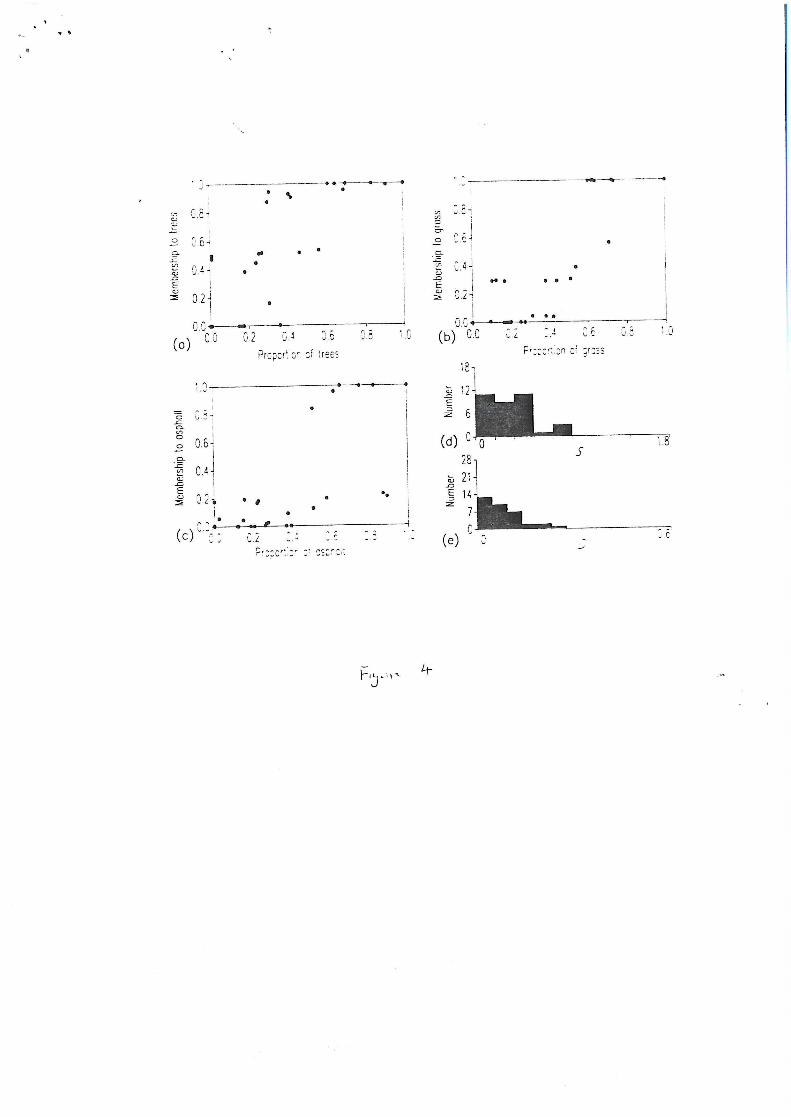
v.L (b) 00

1.3 •

•

0.6J

0.4-

• • • •

41. • • •

0.2 (c) P =U.:2.r CS:r

-2 14

(e) 0 c

Mem

bers

hip t

o as

phalt

.

0.8 -;

0.4

0.2

0.0 (a) 0.0 0.2 C. 0.6 0.8 1.0

Proport.or of trees

0.81

0.6-1

C.4

0.2

0.0

N • •

• •

•

•

•

•

.■ ma • is

Mem

bers

hip t

o tre

es

Mem

bers

hip t

o gr

oss

3.4 0 6 0.8 1.0

Fr::orl.on of grcss

•

•

•

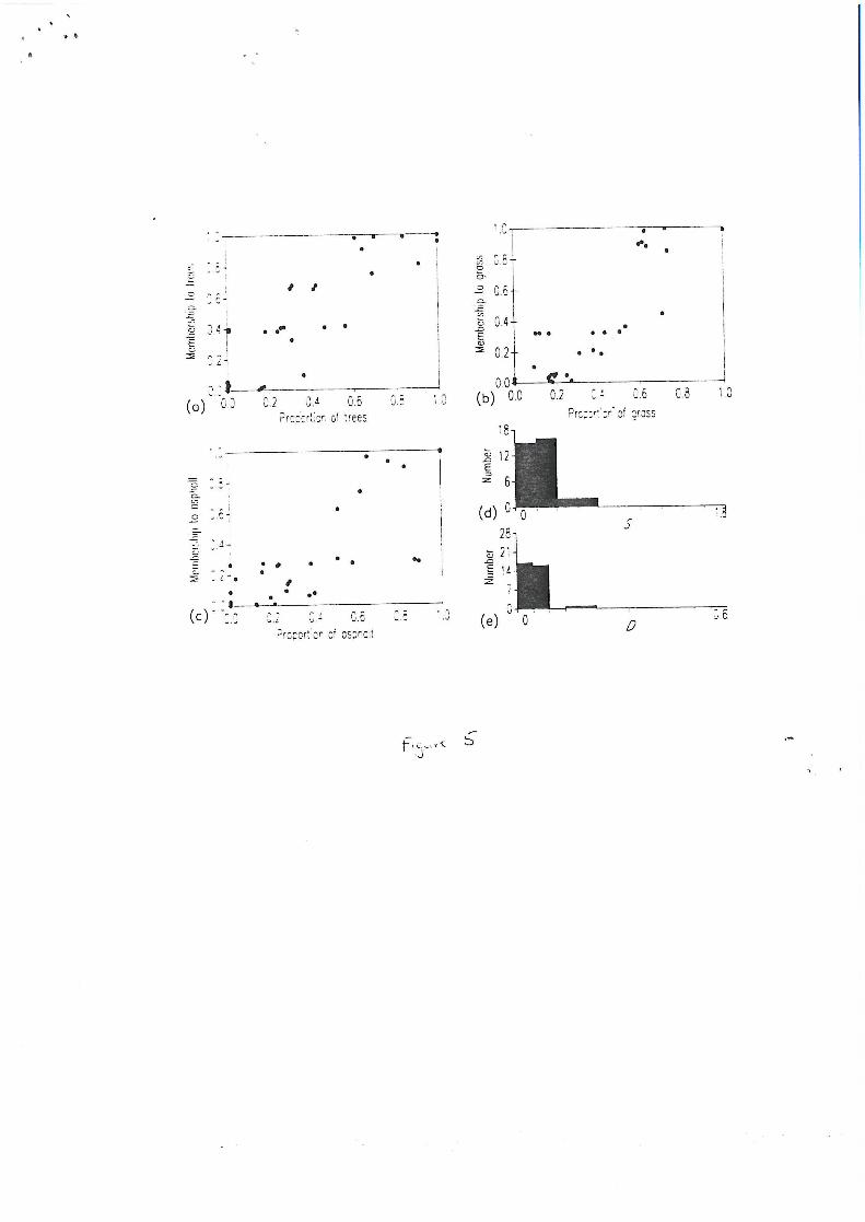
il"

• •• • •

18

12 E

6

(d) 2'8 21

E 14 S.

• • • • • - -

(C) 0.2 0.4 0.6 C. (e)

• • .•

•

T-:ropertior of ospr'.ait

5

O

0.6

a-, 0.4 _.o E

0.2

0.0$ (a) 0.3 0.2 _ 0.4 0.6 0.8 1 0 (b) 0 0

e trees

•

r

•• •

0.2 r 0.6 Pro of crass

0.8 1 0

•

c

. • # •

• • • • •

• • •

(c) , 2.2 ; 2- : CE

0.8 10 0.2 0.4 0.6 PropoHor, of trees

• es

• •

• I.

• •

•

•

S.

•

•

.9 •

0.2 • F. • 41 •

CC C 0.6 08 1.0 p,:cor cr. of gross

18 ,

12- C P 6

d °

28 •,z 21 -S 14

• 6 • • • • •

(b) CC

•

(e) Prop:or...co zsoncA

•

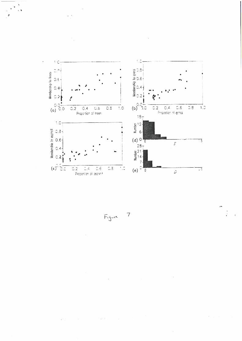
031 (a) 0.0 0.2 0.4 U.b 0.6 1

Proportion of frees

(b) 1.0 0.2 0.4 0.6 3.8 1.0 i7f 9(1,-1

18T

7

Mem

bers

hip

to b

lies

• .5

• s•• • • •

•

•

• • •

0 2 •

•• •

• • $. ■04. •

••

••• •

C,

•••

12 E

6

• (d) 0 • •

• 287 • • 21 . e•

•• 1 4

7

0.2 .1. 4 0.6 Prc;ortion of 3sor,nit

(e)

0

• • • 4'

S

Foody, Giles M. (1996) Approaches for the production and ...

Documents

Transcript of Foody, Giles M. (1996) Approaches for the production and ...