Following Gaze in Video

Adria Recasens Carl Vondrick Aditya Khosla Antonio Torralba

Massachusetts Institute of Technology

{recasens, vondrick, khosla, torralba}@csail.mit.edu

0.8

0a)

b)

c) d)-20 -10 10 20 Frames

Ga

ze

sco

re

0.5

0

Figure 1: a) What is Tom Hanks looking at? When we watch a movie, understanding what a character is paying attention to

requires reasoning about multiple views. Many times, the character will be looking at something that fall outside the frame,

just like in (a), and detecting what object the character is looking at can not be addressed by previous saliency and gaze

following models. Solving this problem requires analyzing gaze, making use of semantic knowledge about the typical 3D

relationships between different views, and recognizing the objects that are the common targets of attention, just like we do

when watching a movie. Here we study the problem of gaze following in video where the object attended by a character

might appear only on a separate frame. Given a video (b) around the frame containing the character (t = 0) our system

selects the frames likely to contain the object attended by the selected character (c) and produces the output shown in (d).

This figure shows an actual result from our system.

AbstractFollowing the gaze of people inside videos is an impor-

tant signal for understanding people and their actions. In

this paper, we present an approach for following gaze in

video by predicting where a person (in the video) is look-

ing even when the object is in a different frame. We collect

VideoGaze, a new dataset which we use as a benchmark to

both train and evaluate models. Given one frame with a

person in it, our model estimates a density for gaze location

in every frame and the probability that the person is look-

ing in that particular frame. A key aspect of our approach

is an end-to-end model that jointly estimates: saliency, gaze

pose, and geometric relationships between views while only

using gaze as supervision. Visualizations suggest that the

model learns to internally solve these intermediate tasks

automatically without additional supervision. Experiments

show that our approach follows gaze in video better than

existing approaches, enabling a richer understanding of hu-

man activities in video.

1. Introduction

Can you tell where Tom Hanks (in Fig. 1(a)) is looking?

You might observe that there is not enough information in

the frame to predict the location of his gaze. However, if we

search the neighboring frames of the given video (shown

in Fig. 1(b)), we can identify he is looking at the woman

(illustrated in Fig. 1(d)). In this paper, we introduce the

problem of gaze following in video. Specifically, given a

video frame with a person, and a set of neighboring frames

from the same video, our goal is to identify which of the

neighboring frames (if any) contain the object being looked

at, and the location on that object that is being gazed upon.

Importantly, we observe that this task requires both a

semantic and geometric understanding of the video. For

example, semantic understanding is required to identify

frames that are from the same scene (e.g., indoor and

outdoor frames are unlikely to be from the same scene)

while geometric understanding is required to localize ex-

actly where the person is looking in a novel frame using the

head pose and geometric relationship between the frames.

Based on this observation, we propose a novel convolu-

tional neural network based model that combines semantic

and geometric understanding of frames to follow an individ-

ual’s gaze in a video. Despite encapsulating the structure of

the problem, our model requires minimal supervision and

produces an interpretable representation of the problem.

In order to train and evaluate our model, we collect

1435

Figure 2: VideoGaze Dataset: We present a novel large-scale dataset for gaze-following in video. Every person annotated

in the dataset has its gaze annotated in five neighbor frames. We show some annotated examples from the dataset. In red, the

frames without the gazed object on it. In green, we show the gaze annotations from the dataset.

a large scale dataset for gaze following in videos. Our

dataset consists of around 50,000 people in short videos an-

notated with where they are looking throughout the video.

We evaluate the performance of a variety of baseline ap-

proaches (e.g., saliency, gaze prediction in images, etc) on

our dataset, and show that our model outperforms all exist-

ing approaches.

There are three main contributions of this paper. First,

we introduce the problem of following gaze in videos. Sec-

ond, we collect a large scale dataset for both training and

evaluation on this task. Third, we present a novel net-

work architecture that leverages the geometry of the scene

to tackle this problem. The remainder of this paper details

these contributions. In Section 2 we explore related work.

In Section 3 we describe our dataset, VideoGaze. In Sec-

tion 4, we describe the model in detail, and finally in Sec-

tion 5 we evaluate the model and provide sample results.

2. Related Work

We describe the related works in the areas of gaze-

following in both videos and images, deep learning for ge-

ometry prediction and saliency below.

Gaze-following in video: Previous works video gaze-

following deal with very restricted settings. Most no-

tably [21, 20] tackles the problem of detecting people look-

ing at each other in video, by using their head pose and loca-

tion inside the frame. Although our model can be used with

this goal, it is applicable to a wide variety of settings: it can

predict gaze when it is located elsewhere in the image (not

only on humans) or future/past frame of the video. Mukher-

jee and Robertson [22] use RGB-D images to predict gaze

in images and videos. They estimate the head-pose of the

person using the multi-modal RGB-D data, and finally they

regress the gaze location with a second system. Although

the output of their system is gaze location, our model does

not need multi-modal data and it is able to deal with gaze

location in a different view. Extensive work has been done

on human interaction and social prediction on both images

and video involving gaze [33, 13, 4]. Some of this work is

focused on ego-centric camera data, such as in [9, 8]. Fur-

thermore, [24, 30] predicts social saliency, that is, the region

that attracts attentions of a group of people in the image. Fi-

nally, [4] estimates the 3D location and pose of the people,

which is used to predict social interaction. Although their

goal is completely different, we also model the scene with

explicit 3D and use it to predict gaze.

Gaze-following in images: Our model is inspired by a

previous gaze-following model for static images [26]. How-

ever, the previous work focuses only on cases where a per-

son, within the image, is looking at another object in the

same image. In this work, we remove this restriction and

extend gaze following to video. The model proposed in

this paper deals with the situation where the person is look-

ing at another frame in the video. Further, unlike [26], we

use parametrized geometry transformations that help the

model to deal with the underlying geometry of the world.

There have also been recent works in applying deep learn-

ing to eye-tracking [16, 35] that predict where an individ-

ual is looking on a device. Furthermore, [32] introduces an

eye-tracking technique which makes the calibration process

avoidable. Finally, our work is also related to [5], which

predicts the object of interaction in images.

Deep Learning with Geometry: Neural networks

have previously been used to model geometric transforma-

1436

target frame xi

head xh

head location ue

Saliency Pathway S(xi)

Gaze PathwayC(xh, ue)

Cone-PlaneIntersection

FC

target frame xt

source frame xs!transformation

Transformation PathwayT(xt, xs)

T1

T2

gaze prediction ŷ

"

Frame Selector

frame probability

Figure 3: Network Architecture: Our model has three pathways. The saliency pathway (top left) finds salient spots on the

target view. The gaze pathway (bottom left) computes the parameters of the cone coming out from the person’s face. The

transformation pathway (right) estimates the geometric relationship between views. The output is the gaze location density

and the probability of xt of containing the gazed object.

tions [11, 12]. Our work is also related to Spatial Trans-

formers Networks [14], where a localization module gen-

erates the parameters of an affine transformation and warps

the representation with bilinear interpolation. Our model

generates parameters of a 3D affine transformation, but

the transformation is applied analytically without warping,

which is likely to be more stable. [28, 6] used 2D images to

learn the underlying 3D structure. Similarly, we expect our

model to learn the 3D structure of the frame composition

only using 2D images. Finally, [10] provide efficient imple-

mentations for adding geometric transformations to CNNs.

Saliency: Although related, gaze-following and free-

viewing saliency refer to different problems. In gaze-

following, we predict the location of the gaze of an ob-

server in the scene, while in saliency we predict the fixa-

tions of an external observer free-viewing the image. Some

authors have used gaze to improve saliency prediction, such

as in [25]. Furthermore, [2] showed how gaze prediction

can improve state-of-the-art saliency models. Although our

approach is not intended to solve video saliency, we be-

lieve it is worth mentioning some works learning saliency

for videos such as [18, 34, 19].

3. VideoGaze Dataset

We introduce VideoGaze, a large scale dataset con-

taining the location where film characters are looking in

movies. VideoGaze contains 166, 721 annotations from

140 movies. To build the dataset we used videos from the

MovieQA dataset [31], which we consider a representative

selection of movies. Each sample of the dataset consists of

six frames. The first frame contains the character whose

gaze is annotated. Eye location and a head bounding box

for the character are provided. The other five frames contain

the gaze location that the character is looking at the time, if

present in the frame. Figure 2 contains three samples from

the dataset. On the left column we show the frame with the

character on it. The other five frames are shown in the right

with the gaze annotation if available (green).

To annotate the dataset, we used Amazon’s Mechani-

cal Turk (AMT). We annotated our dataset in two separate

steps. In the first step, the workers were asked to first locate

the head of the character and then scan through the video

to find the location of the object the character is looking

at. For cost efficiency reasons, we restricted the workers to

only scan a 6 seconds temporal window around the frame

with the character. In pilot experiments, we found this win-

dow to be sufficient. We also provided options to indicate

that the gazed object never appears in the clip or that the

head of the character was not visible in the scene. In the

second step, we temporally sampled four additional frames

nearby the first annotated frame and ask the Turkers to an-

notate the gazed object if present. Using this two-step pro-

cess we ensure that if the gazed object appears in the video,

it is annotated in our VideoGaze.

We split our data into training set and test set. We use

all the annotations from 20 movies as the testing set and the

rest of the annotations as training set. Note that we made the

train/test split by source movie, not by clip, which prevents

overfitting to particular movies. Additionally, we annotated

five times one frame per each sample in the test set. We

used this data to perform a robust evaluation of our methods

and compute a human performance. Finally, for the same

frames, we also annotated the similarity between the frame

with the character and the frame with the object. In figure

8 we use the similarity annotation to evaluate performance

versus different levels of similarity.

4. Method

Suppose we have a video and a person inside the video.

Our goal is to predict where the person is looking, which

1437

!

"

#$ systemofcoordinates #% systemofcoordinates

&(() , +,)

#$ #%

G(+., +/ , ())T(+., +/)

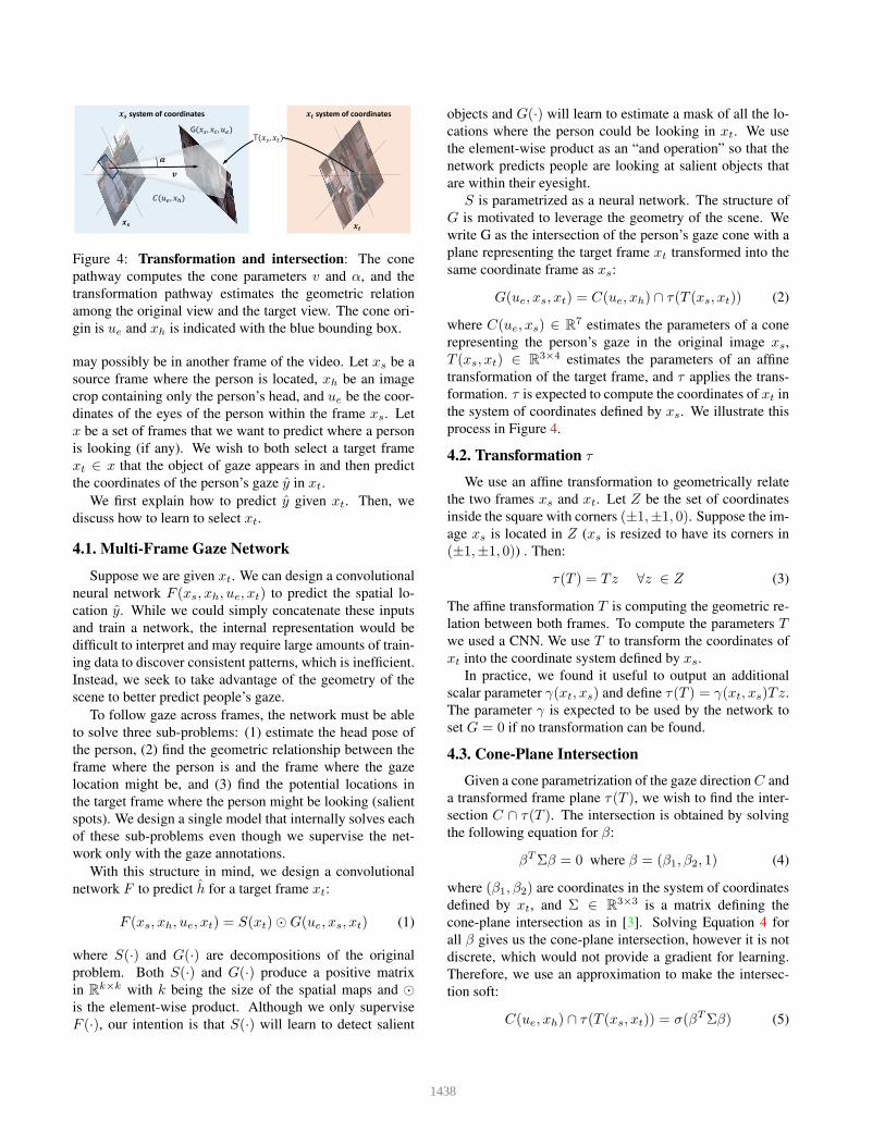
Figure 4: Transformation and intersection: The cone

pathway computes the cone parameters v and α, and the

transformation pathway estimates the geometric relation

among the original view and the target view. The cone ori-

gin is ue and xh is indicated with the blue bounding box.

may possibly be in another frame of the video. Let xs be a

source frame where the person is located, xh be an image

crop containing only the person’s head, and ue be the coor-

dinates of the eyes of the person within the frame xs. Let

x be a set of frames that we want to predict where a person

is looking (if any). We wish to both select a target frame

xt 2 x that the object of gaze appears in and then predict

the coordinates of the person’s gaze y in xt.

We first explain how to predict y given xt. Then, we

discuss how to learn to select xt.

4.1. Multi-Frame Gaze Network

Suppose we are given xt. We can design a convolutional

neural network F (xs, xh, ue, xt) to predict the spatial lo-

cation y. While we could simply concatenate these inputs

and train a network, the internal representation would be

difficult to interpret and may require large amounts of train-

ing data to discover consistent patterns, which is inefficient.

Instead, we seek to take advantage of the geometry of the

scene to better predict people’s gaze.

To follow gaze across frames, the network must be able

to solve three sub-problems: (1) estimate the head pose of

the person, (2) find the geometric relationship between the

frame where the person is and the frame where the gaze

location might be, and (3) find the potential locations in

the target frame where the person might be looking (salient

spots). We design a single model that internally solves each

of these sub-problems even though we supervise the net-

work only with the gaze annotations.

With this structure in mind, we design a convolutional

network F to predict h for a target frame xt:

F (xs, xh, ue, xt) = S(xt)"G(ue, xs, xt) (1)

where S(·) and G(·) are decompositions of the original

problem. Both S(·) and G(·) produce a positive matrix

in Rk×k with k being the size of the spatial maps and "

is the element-wise product. Although we only supervise

F (·), our intention is that S(·) will learn to detect salient

objects and G(·) will learn to estimate a mask of all the lo-

cations where the person could be looking in xt. We use

the element-wise product as an “and operation” so that the

network predicts people are looking at salient objects that

are within their eyesight.

S is parametrized as a neural network. The structure of

G is motivated to leverage the geometry of the scene. We

write G as the intersection of the person’s gaze cone with a

plane representing the target frame xt transformed into the

same coordinate frame as xs:

G(ue, xs, xt) = C(ue, xh) \ τ(T (xs, xt)) (2)

where C(ue, xs) 2 R7 estimates the parameters of a cone

representing the person’s gaze in the original image xs,

T (xs, xt) 2 R3×4 estimates the parameters of an affine

transformation of the target frame, and τ applies the trans-

formation. τ is expected to compute the coordinates of xt in

the system of coordinates defined by xs. We illustrate this

process in Figure 4.

4.2. Transformation τ

We use an affine transformation to geometrically relate

the two frames xs and xt. Let Z be the set of coordinates

inside the square with corners (±1,±1, 0). Suppose the im-

age xs is located in Z (xs is resized to have its corners in

(±1,±1, 0)) . Then:

τ(T ) = Tz 8z 2 Z (3)

The affine transformation T is computing the geometric re-

lation between both frames. To compute the parameters T

we used a CNN. We use T to transform the coordinates of

xt into the coordinate system defined by xs.

In practice, we found it useful to output an additional

scalar parameter γ(xt, xs) and define τ(T ) = γ(xt, xs)Tz.

The parameter γ is expected to be used by the network to

set G = 0 if no transformation can be found.

4.3. Cone-Plane Intersection

Given a cone parametrization of the gaze direction C and

a transformed frame plane τ(T ), we wish to find the inter-

section C \ τ(T ). The intersection is obtained by solving

the following equation for β:

βTΣβ = 0 where β = (β1, β2, 1) (4)

where (β1, β2) are coordinates in the system of coordinates

defined by xt, and Σ 2 R3×3 is a matrix defining the

cone-plane intersection as in [3]. Solving Equation 4 for

all β gives us the cone-plane intersection, however it is not

discrete, which would not provide a gradient for learning.

Therefore, we use an approximation to make the intersec-

tion soft:

C(ue, xh) \ τ(T (xs, xt)) = σ(βTΣβ) (5)

1438

where σ is a sigmoid activation function. To compute the

intersection, we calculate Equation 5 for β1, β2 2 [−1, 1].

4.4. Frame Selection

We described an approach to predict the spatial loca-

tion y where a person is looking inside a given frame xt.

However, how should we pick the target frame xt? To

do this, we can simultaneously estimate the probability

the person of interest is looking inside a frame xt. Let

E (S(xt), G(ue, xs, xt)) be this probability where E is a

neural network.

4.5. Pathways

We estimate the parameters of the saliency map S, the

cone C, and the transformation T using CNNs.

Saliency Pathway: The saliency pathway uses the target

frame xt to generate a spatial map S(xt). We used a 6-

layer CNN to generate the spatial map from the input image.

The five initial convolutional layers follow the structure of

AlexNet introduced by [17]. The last layer uses a 1 ⇥ 1kernel to merge the 256 channels in a simple k ⇥ k map.

Cone Pathway: The cone pathway generates a cone

parametrization from a close-up image of the head xh and

the eyes ue. We set the origin of the cone at the head of

the person ue and let a CNN generate v 2 R3, the direc-

tion of the cone and α 2 R, its aperture. Figure 4 shows an

schematic example of the cone generation.

Transformation Pathway: The transformation pathway

has two stages. We define T1, a 5-layer CNN following

the structure defined in [17]. T1 is applied separately to

both the source frame xs and the target frame xt. We define

T2 which is composed by one convolutional layer and three

fully connected layers reducing the dimensionality of the

representation. The output of the pathway is computed as:

T (xs, xt) = T2(T1(xs), T1(xt)). We used [10] to compute

the transformation matrix from output parameters.

Discussion: We constrain each pathway to learn differ-

ent aspects of the problem by providing each pathway only

a subset of the inputs. The saliency pathway only has ac-

cess to the target frame xt, which is insufficient to solve the

full problem. Instead, we expect it to find salient objects in

the target view xt. Likewise, the transformation pathway

has access to both xs and xt, and the transformation will be

later used to project the gaze cone. We expect it to com-

pute a transformation that geometrically relates xs and xt.

We expect each of the pathways to solve its particular sub-

problem to then get combined to generate the final output.

Since every step is differentiable, it can be trained end-to-

end without intermediate supervision.

4.6. Learning

Since gaze-following is a multi-modal problem, we train

F to estimate a spatial probability distribution q(x, y) in-

stead of regressing a single gaze location. We use a gen-

eralization of the spatial loss used in [26]. They use five

different classification grids that are shifted and the predic-

tions of each of them are combined. We generalize this loss

by averaging over all the possible grids of different shifts

and sizes:

L(p, q) =X

w,h,∆x,∆y

Ew,h,∆x,∆y(p, q) (6)

where Ew,h,∆x,∆yis a spatially smooth cross entropy with

grid cells sized w ⇥ h and shifted (∆x,∆y) spaces over.

Instead of using q to compute the loss, E uses a smoothed

version of q where for each position (x, y) it sums up the

probability in the rectangle around. For simplicity, we write

this in one dimension:

Ew,∆x= −

X

x

p(x) log

δ=wX

δ=0

q(x+∆x + δ) (7)

which is similar to the cross-entropy loss function except

the spatial bins are shifted by ∆x and scaled by w. This

expression can be written as the output of a convolution,

which is efficient to compute, and differentiable.

4.7. Inference

Our network F will produce a matrix A 2 R20×20, a

map that can be interpreted as a density where the person

is looking. To infer the gaze location y in the target frame

xt, we find the mode of this density y = argmaxi,j Aij .

To select the target frame xt, we pick the frame with the

highest score from E.

4.8. Implementation Details

We implemented our model using PyTorch. In our ex-

periments we use k = 13, the output of both the saliency

pathway and the cone generator is a 13⇥13 spatial map. We

found useful to add a final fully connected layer to upscale

the 13⇥13 spatial map to a 20⇥20 spatial map. We initial-

ize the CNNs in the three pathways with ImageNet-CNN

[17, 29]. The cone pathway has three fully connected layers

of sizes 500, 200 and 4 to generate the cone parametriza-

tion. The common part of the transformation pathway, T2,

has one convolutional layer with a 1⇥1 kernel and 100 out-

put channels, followed by one 2⇥ 2 max pooling layer and

three fully connected layers of 200, 100 and the parame-

ter size of the transformation. E is a Multilayer Perceptron

with one hidden layer of 200 dimensions. For training, we

augment data by flipping xt and xs and their annotations.

5. Experiments

5.1. Evaluation Procedure

To evaluate our model we conducted quantitative and

qualitative analyses using our held out dataset. We use 4

1439

Model Dist Min.Dist AUC KL

Static Gaze [26] 0.287 0.233 76.5 9.03Saliency 0.253 0.206 85.0 8.49Fixed bias 0.281 0.226 71.0 22.79Center 0.236 0.198 76.3 18.64Random 0.437 0.380 56.9 28.39Ours 0.184 0.123 89.0 7.76

Human 0.103 0.063 90.1 10.59

(a) Baselines

Model Dist Min.Dist AUC KL

Cone Only 0.194 0.139 83.8 8.52Image Only 0.236 0.175 87.7 7.90Identity 0.201 0.141 86.6 8.04Translation Only 0.194 0.133 87.9 7.81Rotation Only 0.195 0.134 87.5 7.95Vertical axis rot 0.189 0.128 88.5 7.823-axis rot (Ours) 0.184 0.123 89.0 7.76

(b) Ablation Analysis

Model AP

Random 75.1Closest 75.7Saliency 76.0Image only 83.9Cone only 86.7Vertical axis rot 87.1Ours 87.5

(c) Frame selection

Table 1: Evaluation: In table (a) we compare our performance with the baselines. In table (b) we analyze the performance

of the different ablations of our model. In table (c) we analyze the ability of the model to select the target frame. We compare

against baselines and ablations. AUC stands for Area Under the Curve and it is computed as the to the area under the ROC

curve. Dist. is computed as the L2 distance to the ground truth location. Min.Dist is computed as the minimum L2 distance

to one ground truth annotation. KL refers to the Kullback-Leibler divergence. AP stands for Average Precision, and is defined

as the area under the precision-recall curve. Higher is better for AUC and AP. Lower is better for KL and L2 distances.

ground truth annotations for evaluations and one to eval-

uate human performance. Similar to [7], for quantitative

evaluation we provide bounding boxes for the heads of the

persons. The bounding boxes are part of the dataset and

have been collected using Amazon’s Mechanical Turk. This

makes the evaluation focused on the gaze following task. In

Figure 7 and 5 we provide some qualitative examples of our

system working with head bounding boxes computed with

an automatic head detector. For our quantitative evaluation,

we report performances of the model in two tasks: predict-

ing the gaze location given the frame with the object, and

selecting the frame with the object.

5.1.1 Predicting gaze location

We use AUC, L2 distances and KL divergence as our eval-

uation metrics for predicting gaze location. AUC refers to

Area Under the Curve, a measure typically used to com-

pare predicted distributions to samples. The predicted heat

map is used as a confidence to build a ROC curve. We used

[15] to compute the AUC metric. We also used L2 metric,

which is computed as the euclidean error between the pre-

dicted point and the ground truth annotation. Additionally,

we report minimum distance to human annotation, which

is the L2 distance for the closer ground truth point. For

comparison purposes, we assume the images are normal-

ized to having sides of length 1 unit. Finally, KL refers to

the Kullback-Leibler divergence, a measure of the informa-

tion lost when the output map is used as the gaze fixation

map. KL is typically used to compare distributions [1].

Previous work in gaze following in video cannot be eval-

uated in our benchmark because of its particular contains

(only predicting social interaction or using multi-model

data). We compare our method to several baselines de-

scribed below. For methods producing a single location, we

used a Gaussian distribution centered in the output location.

Random: The prediction is a random location in the im-

age. Center: The prediction is always the center of the

image. Fixed bias: The head location is quantized in a

13 ⇥ 13 grid and the training set is used to compute the

average output location per each head location. Saliency:

The output heatmap is the saliency prediction for xt. [23]

is used to compute the saliency map. The output point is

computed as the mode of the saliency output distribution.

Static Gaze: [26] is used to compute the gaze prediction.

Since it is a method for static images, the head image and

the head location provided are from the source view but the

image provided is the target view.

Additionally, we performed an analysis on the compo-

nents of our model. With this analysis, we aim to under-

stand the contribution of each of the parts to performance

as well as suggest that all of them are needed.

Translation only: The affine transformation is a trans-

lation. Rotation only: The affine transformation is a 3-axis

rotation. Identity: The affine transformation is the identity.

Image only: The saliency pathway is used to generate the

output. Cone only: The gaze pathway combined with the

transformation pathway are used to generate the output. 3

axis rotation / translation: The affine transformation is a 3axis rotation combined with a translation. Vertical axis ro-

tation: The affine transformation is a rotation in the vertical

axis combined with a translation.

5.1.2 Frame selection

We use mean Average Precision as our evaluation metric

for the frame selection. AP is defined as the area under the

precision-recall curve and has been extensively used to eval-

uate detection problems. As for predicting the gaze loca-

tion, previous work in gaze-following cannot be applicable

to solve the frame selection task. We compare our method

to the baselines described below.

Random: The score for the frame is randomly assigned.

Closest: The score is inverse to the time difference be-

tween the source frame and the target frame. Saliency: The

score assigned to the frame is inverse to the entropy of the

1440

0-20 -10 10 20 Frames30a)b)

Frames

0.8

Ga

ze

sco

re

0.5

0

c)

0.7

Ga

ze

sco

re 0.5

00-20 -10 10 20 30 d)

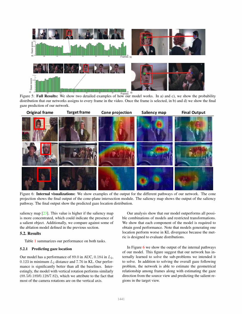
Figure 5: Full Results: We show two detailed examples of how our model works. In a) and c), we show the probability

distribution that our networks assigns to every frame in the video. Once the frame is selected, in b) and d) we show the final

gaze prediction of our network.

Originalframe Targetframe Coneprojection Saliencymap FinalOutput

Figure 6: Internal visualizations: We show examples of the output for the different pathways of our network. The cone

projection shows the final output of the cone-plane intersection module. The saliency map shows the output of the saliency

pathway. The final output show the predicted gaze location distribution.

saliency map [23]. This value is higher if the saliency map

is more concentrated, which could indicate the presence of

a salient object. Additionally, we compare against some of

the ablation model defined in the previous section.

5.2. Results

Table 1 summarizes our performance on both tasks.

5.2.1 Predicting gaze location

Our model has a performance of 89.0 in AUC, 0.184 in L2,

0.123 in minimum L2 distance and 7.76 in KL. Our perfor-

mance is significantly better than all the baselines. Inter-

estingly, the model with vertical rotation performs similarly

(88.5/0.189/0.128/7.82), which we attribute to the fact that

most of the camera rotations are on the vertical axis.

Our analysis show that our model outperforms all possi-

ble combinations of models and restricted transformations.

We show that each component of the model is required to

obtain good performance. Note that models generating one

location perform worse in KL divergence because the met-

ric is designed to evaluate distributions.

In Figure 6 we show the output of the internal pathways

of our model. This figure suggest that our network has in-

ternally learned to solve the sub-problems we intended it

to solve. In addition to solving the overall gaze following

problem, the network is able to estimate the geometrical

relationship among frames along with estimating the gaze

direction from the source view and predicting the salient re-

gions in the target view.

1441

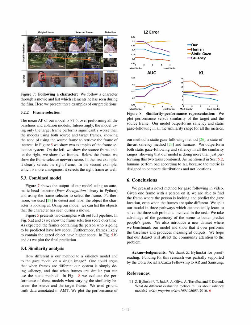
Originalframe Selectedframe Detection

Failures

GoodPredictions

Person

Person

Car

Figure 7: Following a character: We follow a character

through a movie and list which elements he has seen during

the film. Here we present three examples of our predictions.

5.2.2 Frame selection

The mean AP of our model is 87.5, over performing all the

baselines and ablation models. Interestingly, the model us-

ing only the target frame performs significantly worse than

the models using both source and target frames, showing

the need of using the source frame to retrieve the frame of

interest. In Figure 5 we show two examples of the frame se-

lection system. On the left, we show the source frame and,

on the right, we show five frames. Below the frames we

show the frame selector network score. In the first example,

it clearly selects the right frame. In the second example,

which is more ambiguous, it selects the right frame as well.

5.3. Combined model

Figure 7 shows the output of our model using an auto-

matic head detector (Face Recognition library in Python)

and using the frame selector to select the frame. Further-

more, we used [27] to detect and label the object the char-

acter is looking at. Using our model, we can list the objects

that the character has seen during a movie.

Figure 5 presents two examples with out full pipeline. In

Fig. 5.a) and c) we show the frame selection score over time.

As expected, the frames containing the person who is going

to be predicted have low score. Furthermore, frames likely

to contain the gazed object have higher score. In Fig. 5.b)

and d) we plot the final prediction.

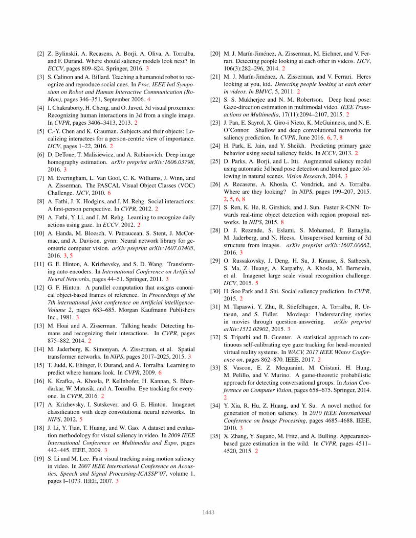
5.4. Similarity analysis

How different is our method to a saliency model and

to the gaze model on a single image? One could argue

that when frames are different our system is simply do-

ing saliency, and that when frames are similar you can

use the static method. In Fig. 8 we evaluate the per-

formance of these models when varying the similarity be-

tween the source and the target frame. We used ground

truth data annotated in AMT. We plot the performance of

AUC

L2Error

KL

MostSimilar LeastSimilar MostSimilar LeastSimilar

MostSimilar LeastSimilar

Figure 8: Similarity-performance representation: We

plot performance versus similarity of the target and the

source frame. Our model outperforms saliency and static

gaze-following in all the similarity range for all the metrics.

our method, a static gaze-following method [26], a state-of-

the-art saliency method [23] and humans. We outperform

both static gaze-following and saliency in all the similarity

ranges, showing that our model is doing more than just per-

forming this two tasks combined. As mentioned in Sec. 5.2,

humans perfom bad according to KL because the metric is

designed to compare distributions and not locations.

6. Conclusions

We present a novel method for gaze following in video.

Given one frame with a person on it, we are able to find

the frame where the person is looking and predict the gaze

location, even when the frames are quite different. We split

our model in three pathways which automatically learn to

solve the three sub problems involved in the task. We take

advantage of the geometry of the scene to better predict

people’s gaze. We also introduce a new dataset where

we benchmark our model and show that it over performs

the baselines and produces meaningful outputs. We hope

that our dataset will attract the community attention to the

problem.

Acknowledgements. We thank Z. Bylinskii for proof-

reading. Funding for this research was partially supported

by the Obra Social la Caixa Fellowship to AR and Samsung.

References

[1] Z. Bylinskii*, T. Judd*, A. Oliva, A. Torralba, and F. Durand.

What do different evaluation metrics tell us about saliency

models? arXiv preprint arXiv:1604.03605, 2016. 6

1442

[2] Z. Bylinskii, A. Recasens, A. Borji, A. Oliva, A. Torralba,

and F. Durand. Where should saliency models look next? In

ECCV, pages 809–824. Springer, 2016. 3

[3] S. Calinon and A. Billard. Teaching a humanoid robot to rec-

ognize and reproduce social cues. In Proc. IEEE Intl Sympo-

sium on Robot and Human Interactive Communication (Ro-

Man), pages 346–351, September 2006. 4

[4] I. Chakraborty, H. Cheng, and O. Javed. 3d visual proxemics:

Recognizing human interactions in 3d from a single image.

In CVPR, pages 3406–3413, 2013. 2

[5] C.-Y. Chen and K. Grauman. Subjects and their objects: Lo-

calizing interactees for a person-centric view of importance.

IJCV, pages 1–22, 2016. 2

[6] D. DeTone, T. Malisiewicz, and A. Rabinovich. Deep image

homography estimation. arXiv preprint arXiv:1606.03798,

2016. 3

[7] M. Everingham, L. Van Gool, C. K. Williams, J. Winn, and

A. Zisserman. The PASCAL Visual Object Classes (VOC)

Challenge. IJCV, 2010. 6

[8] A. Fathi, J. K. Hodgins, and J. M. Rehg. Social interactions:

A first-person perspective. In CVPR, 2012. 2

[9] A. Fathi, Y. Li, and J. M. Rehg. Learning to recognize daily

actions using gaze. In ECCV. 2012. 2

[10] A. Handa, M. Bloesch, V. Patraucean, S. Stent, J. McCor-

mac, and A. Davison. gvnn: Neural network library for ge-

ometric computer vision. arXiv preprint arXiv:1607.07405,

2016. 3, 5

[11] G. E. Hinton, A. Krizhevsky, and S. D. Wang. Transform-

ing auto-encoders. In International Conference on Artificial

Neural Networks, pages 44–51. Springer, 2011. 3

[12] G. F. Hinton. A parallel computation that assigns canoni-

cal object-based frames of reference. In Proceedings of the

7th international joint conference on Artificial intelligence-

Volume 2, pages 683–685. Morgan Kaufmann Publishers

Inc., 1981. 3

[13] M. Hoai and A. Zisserman. Talking heads: Detecting hu-

mans and recognizing their interactions. In CVPR, pages

875–882, 2014. 2

[14] M. Jaderberg, K. Simonyan, A. Zisserman, et al. Spatial

transformer networks. In NIPS, pages 2017–2025, 2015. 3

[15] T. Judd, K. Ehinger, F. Durand, and A. Torralba. Learning to

predict where humans look. In CVPR, 2009. 6

[16] K. Krafka, A. Khosla, P. Kellnhofer, H. Kannan, S. Bhan-

darkar, W. Matusik, and A. Torralba. Eye tracking for every-

one. In CVPR, 2016. 2

[17] A. Krizhevsky, I. Sutskever, and G. E. Hinton. Imagenet

classification with deep convolutional neural networks. In

NIPS, 2012. 5

[18] J. Li, Y. Tian, T. Huang, and W. Gao. A dataset and evalua-

tion methodology for visual saliency in video. In 2009 IEEE

International Conference on Multimedia and Expo, pages

442–445. IEEE, 2009. 3

[19] S. Li and M. Lee. Fast visual tracking using motion saliency

in video. In 2007 IEEE International Conference on Acous-

tics, Speech and Signal Processing-ICASSP’07, volume 1,

pages I–1073. IEEE, 2007. 3

[20] M. J. Marın-Jimenez, A. Zisserman, M. Eichner, and V. Fer-

rari. Detecting people looking at each other in videos. IJCV,

106(3):282–296, 2014. 2

[21] M. J. Marın-Jimenez, A. Zisserman, and V. Ferrari. Heres

looking at you, kid. Detecting people looking at each other

in videos. In BMVC, 5, 2011. 2

[22] S. S. Mukherjee and N. M. Robertson. Deep head pose:

Gaze-direction estimation in multimodal video. IEEE Trans-

actions on Multimedia, 17(11):2094–2107, 2015. 2

[23] J. Pan, E. Sayrol, X. Giro-i Nieto, K. McGuinness, and N. E.

O’Connor. Shallow and deep convolutional networks for

saliency prediction. In CVPR, June 2016. 6, 7, 8

[24] H. Park, E. Jain, and Y. Sheikh. Predicting primary gaze

behavior using social saliency fields. In ICCV, 2013. 2

[25] D. Parks, A. Borji, and L. Itti. Augmented saliency model

using automatic 3d head pose detection and learned gaze fol-

lowing in natural scenes. Vision Research, 2014. 3

[26] A. Recasens, A. Khosla, C. Vondrick, and A. Torralba.

Where are they looking? In NIPS, pages 199–207, 2015.

2, 5, 6, 8

[27] S. Ren, K. He, R. Girshick, and J. Sun. Faster R-CNN: To-

wards real-time object detection with region proposal net-

works. In NIPS, 2015. 8

[28] D. J. Rezende, S. Eslami, S. Mohamed, P. Battaglia,

M. Jaderberg, and N. Heess. Unsupervised learning of 3d

structure from images. arXiv preprint arXiv:1607.00662,

2016. 3

[29] O. Russakovsky, J. Deng, H. Su, J. Krause, S. Satheesh,

S. Ma, Z. Huang, A. Karpathy, A. Khosla, M. Bernstein,

et al. Imagenet large scale visual recognition challenge.

IJCV, 2015. 5

[30] H. Soo Park and J. Shi. Social saliency prediction. In CVPR,

2015. 2

[31] M. Tapaswi, Y. Zhu, R. Stiefelhagen, A. Torralba, R. Ur-

tasun, and S. Fidler. Movieqa: Understanding stories

in movies through question-answering. arXiv preprint

arXiv:1512.02902, 2015. 3

[32] S. Tripathi and B. Guenter. A statistical approach to con-

tinuous self-calibrating eye gaze tracking for head-mounted

virtual reality systems. In WACV, 2017 IEEE Winter Confer-

ence on, pages 862–870. IEEE, 2017. 2

[33] S. Vascon, E. Z. Mequanint, M. Cristani, H. Hung,

M. Pelillo, and V. Murino. A game-theoretic probabilistic

approach for detecting conversational groups. In Asian Con-

ference on Computer Vision, pages 658–675. Springer, 2014.

2

[34] Y. Xia, R. Hu, Z. Huang, and Y. Su. A novel method for

generation of motion saliency. In 2010 IEEE International

Conference on Image Processing, pages 4685–4688. IEEE,

2010. 3

[35] X. Zhang, Y. Sugano, M. Fritz, and A. Bulling. Appearance-

based gaze estimation in the wild. In CVPR, pages 4511–

4520, 2015. 2

1443