Focal mechanism determination of induced microearthquakes in an oilfield using full waveforms from shallow and deep seismic networks

Junlun Li1, H. Sadi Kuleli1, Haijiang Zhang1, and M. Nafi Toksoz1

ABSTRACT

A new, relatively high frequency, full waveform matchingmethod was used to study the focal mechanisms of small, localearthquakes induced in an oil field, which are monitored by asparse near-surface network and a deep borehole network. Thedetermined source properties are helpful for understanding thelocal stress regime in this field. During the waveform inversion,wemaximize both the phase and amplitudematching between theobserved and modeled waveforms. We also use the polarities ofthe first P-wave arrivals and the average S/P amplitude ratios tobetter constrain the matching. An objective function is con-structed to include all four criteria. For different hypocentersand source types, comprehensive synthetic tests showed thatour method is robust enough to determine the focal mechanisms

under the current array geometries, even when there is consider-able velocity inaccuracy. The application to several tens of in-duced microseismic events showed satisfactory waveformmatching between modeled and observed seismograms. Mostof the events have a strike direction parallel with the major north-east-southwest faults in the region, and some events trend parallelwith thenorthwest-southeast conjugate faults.The results are con-sistentwith the in situwell breakoutmeasurements and the currentknowledge on the stress direction of this region. The source me-chanisms of the studied events, together with the hypocenter dis-tribution, indicate that the microearthquakes are caused by thereactivation of preexisting faults. We observed that the faultingmechanism varies with depth, from strike-slip dominance at shal-lower depth to normal faulting dominance at greater depth.

INTRODUCTION

Induced seismicity is a common phenomenon in oil/gas reser-voirs accompanying changes in internal stress due to water injectionor water/oil/gas extraction, etc. (e.g., Suckale, 2010; Maxwell et al.,2010). For example, the gas/oil extraction can cause reservoir com-paction and reactivate preexisting faults and induce microearth-quakes (e.g., Chan and Zoback, 2007; Miyazawa et al., 2008;Sarkar et al., 2008), or injection of water can cause the decrease ofeffective stress and slippage along preexisting faults (Grasso, 1992).The reactivation of preexisting faults is very likely responsible forthe sheared casings of production wells in some fields (Maury et al.,1992) or is a serious source of wellbore instability during drillings(Willson et al., 1998; Zoback and Zinke, 2002). The hydraulic frac-turing activities in an enhanced geothermal system or in shale gasextraction can also result in crack openings and closures and induce

microseismicity (Baig and Urbancic, 2010). Through the studyingof locations and source characteristics (e.g., focal mechanism) ofthe induced seismicity over an extended time period, temporal andspatial changes of the stress in the fields may be reconstructed; thiscan help to understand the intrinsic response of geological forma-tions to the stress disturbance.Microearthquakes usually have small magnitudes and are gener-

ally recorded at sparse local stations. As a result, it is difficult toobtain enough seismic waveforms with high signal-to-noise ratiofor picking the polarity information of first P-wave arrivals. There-fore, it is challenging to use only the P-wave polarity information(even when adding S/P amplitude ratios) as used in conventionalmethods to constrain the focal mechanisms of the induced earth-quakes (e.g., Hardebeck and Shearer, 2002, 2003), especially whenthere are only a limited number of stations. Waveform matching hasbeen used to determine earthquake focal mechanisms on a regional

Manuscript received by the Editor 31 January 2011; revised manuscript received 9 May 2011; published online 27 December 2011; corrected version pub-lished online 18 January 2012.

1Massachusetts Institute of Technology, Earth Resources Laboratory, Department of Earth, Atmospheric, and Planetary Sciences, Cambridge, Massachusetts,USA. E-mail: junlunli@mit.edu; kuleli@mit.edu; hjzhang@mit.edu; toksoz@mit.edu.© 2011 Society of Exploration Geophysicists. All rights reserved.

WC87

GEOPHYSICS. VOL. 76, NO. 6 (NOVEMBER-DECEMBER 2011); P. WC87–WC101, 13 FIGS., 3 TABLES.10.1190/GEO2011-0030.1

Downloaded 24 Jan 2012 to 18.111.29.106. Redistribution subject to SEG license or copyright; see Terms of Use at http://segdl.org/

and global scale using low frequency waveform information(e.g., Šílený et al., 1992; Zhao and Helmberger, 1994; Tan andHelmberger, 2007). Šílený et al. (1992) use waveform matchingto determine the best-fit focal mechanism, source time functionand source depth. Zhao and Helmberger (1994) allowed time-shiftin the synthetic seismograms to account for the imperfect Green’sfunctions when matching the synthetic with observed seismograms.Tan and Helmberger (2007) match the direct P-arrival phases (thefirst whole cycle after initial P-arrival) between synthetic and ob-served seismograms to determine the focal mechanisms. However,in the case of induced seismicity, waveforms usually have higherfrequencies. There have been many studies on determining the focalmechanism of the induced seismicity in the cases of enhancedgeothermal system development, mining, and hydraulic fracturing.Godano et al. (2011) use the direct amplitudes of P, SV, and SH tostudy the focal mechanisms of induced microearthquakes in ageothermal site using full-space homogeneous velocity models.Nolen-Hoeksema et al. (2001) use the first half cycle after the firstarrivals from the observed seismograms and synthetics from full-space Green’s functions to determine the focal mechanisms of sev-eral hydraulic fracture events. Julian et al. (2007) use first arrivalpolarities and amplitude ratios from 16 three-component boreholestations and 14 three-component surface stations to determine thefull moment tensors of the induced events and studied the volumechange accompanying the geothermal process. High frequencywaveform matching, in addition to polarity information, has beenused to determine the focal mechanisms of induced earthquakes in amine with a dense network of 20 stations (Julià and Nyblade, 2009).Julià and Nyblade (2009) use a full-space homogeneous model tocalculate the Green’s functions, and they performed the focal me-chanism inversion in the frequency domain without phase informa-tion in a least-squares sense between the synthetic and filteredobserved data generally below 10 Hz. The simplification to thefull-space homogeneous model is valid when the receivers are de-ployed deep in the subsurface and close to the induced events, suchas deploying borehole monitoring sensors in the vicinity of the hy-draulic well, or when complexities in rock structure are not largecompared to the frequencies recorded.To retrieve reliable solutions, we developed a method to use high-

frequency, full waveform information (both P and S) to determinethe focal mechanisms of small earthquakes (Li et al., 2011). Usingthe known velocity model (one-dimensional layered model in thisstudy), we calculate the Green’s functions for all moment tensorcomponents of the source at each location (hypocenter) and thenthe synthetic seismograms by convolving them with the source timefunction. To find the best match between the observed and syntheticseismograms, we formulate an objective function that incorporatesinformation from different attributes in the waveforms: the cross-correlation values between the modeled waveforms and the data,the L2 norms of the waveform differences, and the polarities ofthe first P arrivals and the S/P average amplitude ratios. Comparedto previous studies, our method uses more attributes of seismogramsto better determine the focal mechanisms of induced seismicity. The“high frequency” referred to in our study (several hertz for the shal-low network and tens of hertz for the deep network) is a relativeterm: it is much higher than the frequency band (0.05–0.5 Hz) oftenused in the study of large earthquakes (e.g., Tan and Helmberger,2007), but it is lower than the frequency band often used forexploration seismic imaging (e.g., Etgen et al., 2009). Essentially,

the frequency bands used in our study include a considerable por-tion of the energy radiated from the source; thus, the waveformshave good signal-to-noise ratio (S/N) and can reflect the character-izations of the source rupture.Compared with full waveform tomography or migration tech-

niques, which focus on improving the knowledge of the subsurfacestructures illuminated by simple active sources with known signa-tures (e.g., explosion or vibration source with known location andorigin time; similar frequency, amplitude, radiation pattern, etc., areexpected for all shots), the source mechanism determination methodassumes the velocity model input, and focuses on determining thecomplicated source signature associated with the events. Forinduced seismicity in oil and gas fields, the velocity model is gen-erally known from seismics and well logs. Comprehensive synthetictests with random velocity perturbations are also performed to ex-amine the robustness of our algorithm in the presence of the velocityuncertainties.Previously, we tested our newly developed focal mechanism

determination method on induced microearthquakes monitoredby a five-station surface network at an oil field in Oman (Li et al.,2011). The field, operated by Petroleum Development Oman(PDO), was discovered in 1962 and put into production in 1969.An official program to monitor induced seismicity using a surfacestation network in the field commenced in 1999, and a boreholenetwork was installed in February of 2002. The primary objectiveof this passive seismicity monitoring program was to locate theevents and to correlate them with production and injection activitiesto understand and monitor the cause of induced seismicity in thefield. In this paper, we apply the newly developed focal mechanismdetermination method to data from the borehole network. Thesource mechanisms determined using the borehole network arecompared to those determined using the surface network. The ro-bustness of the method is tested extensively on synthetic data setsgenerated for both the surface and borehole networks using a ran-domly perturbed velocity model.

INDUCED MICROEARTHQUAKE DATA SET

The petroleum field discussed in this paper is a large anticlinecreated by deep-seated salt movement (Sarkar, 2008). The domeis about 15 × 20 km in size with a northeast-southwest axial elon-gation that is probably a result of regional deformation. The struc-ture is dominated by a major central graben and two systems offaulting with two preferred directions (southeast-northwest andnortheast-southwest) that affect the trapping mechanism in theoil reservoir. The northeast-southwest major network of faults andfractures partially connects all parts of the fields (Figures 1, 2). Themain oil production is from the Lower Cretaceous Shuaiba chalkoverlain unconformably by Nahr Umr shale, while gas isproduced from the shallower Natih Formation overlain by the Fiqashale Formation (Sarkar, 2008; Zhang et al., 2009).Since 1996, increasing seismic activity has been reported by the

staff working in the field. Significant surface subsidence in the cen-ter of the field has also been observed by InSAR, GPS, and levelingsurveys, and has been attributed to compaction of the Natih forma-tion (Bourne et al., 2006). To monitor the induced seismicity in thefield, PDO first deployed a surface array of monitoring stations in1999 (Figure 1). The stations are instrumented with SM-6B geo-phones with a natural frequency (f n) of 4.5 Hz. In 2002, anothernetwork, independent of the shallow network, was installed in

WC88 Li et al.

Downloaded 24 Jan 2012 to 18.111.29.106. Redistribution subject to SEG license or copyright; see Terms of Use at http://segdl.org/

the field as part of a Shell/PDO collaborative study (Figure 2). Un-like the surface array/shallow network, this network had boreholeinstallations of seismic sensors (SM-7m, f n ¼ 30 Hz) at multiplelevels, roughly ranging from depths of 750 to 1250 m. The instru-mentation for this network was much deeper than that of the surfacenetwork, and therefore, this monitoring network is referred to as the“borehole network.” A schematic diagram of the wells and sensorpositions is shown in Figure 2. The borehole network consisted offive closely spaced monitoring wells in the most seismically activepart of the reservoir and covered a much smaller area than the sur-face network. Due to sensor positions at depths, the ability to ac-quire data at much higher frequencies and the proximity to the twoproducing units (Natih gas and Shuaiba oil), the deep network re-corded much smaller magnitude events than the shallow network,resulting in a greatly increased detectability of induced seismicity(roughly about 25 times more induced events per day) compared tothe shallow network. The borehole network was operational forabout 18 months starting in February 2002; however, only micro-seismic data from the last 11 months (October 2002–August 2003)were available for this study. During that 11-month monitoring per-

iod, about 15,800 events were identified with an average rate of∼47∕day, out of which we analyzed and located about 5,400 events(Sarkar, 2008). Attempts were made to select common eventsdetected during this period by both (deep and shallow) networksfor a joint location analysis; however, due to clock synchronizationproblems and difference in sensor frequency bands between the twonetworks, the common events could not be identified, and hence thetask could not be accomplished. Some research indicated that bycarefully identifying the largest events in different networks,synchronization between networks sometimes can be achievedby shifting the origin times in one network with a constant time(Eisner et al., 2010). A similar strategy will be adopted in the future.During the period of 1999 to 2007, over 1500 induced earth-

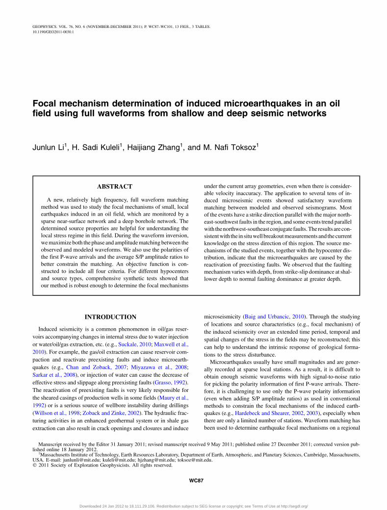
quakes were recorded by the surface network, and their occurrencefrequency was found to be correlated with the amount of gas pro-duction (Sarkar, 2008). The distribution of induced events in thefield recorded by the surface network is shown in Figure 1 (Sarkar,2008; Sarkar et al., 2008; Zhang et al., 2009). All the events have aresidual traveltime of less than 30 ms, indicating they are welllocated. Figure 2 shows the microearthquake locations determinedusing the deep borehole network and the double-differencetomography method (Zhang et al., 2009). The root-mean-square

Figure 1. Distributions of near-surface stations and located events.(a) Map view of the studied field. The blue hexagons (E1, E2, andE3) are the epicenters of synthetic events and the green triangles(VA11, VA21, VA31, VA41, and VA51) are the five near-surfacestations. These stations are located in shallow boreholes, 150 m be-low the surface, to increase the signal-to-noise ratio (S/N). Theblack lines are the identified faults. (b) Side view of the studiedfield. Most of the induced microearthquakes are localized around1 km below the surface. A few shallow events have the largest tra-veltime residues among all events.

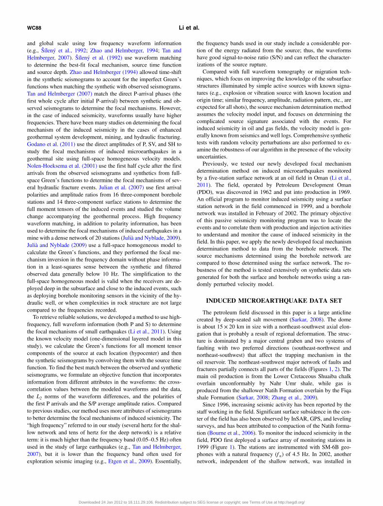
Figure 2. (a) Map view of the borehole network and the microearth-quakes located by this network. The yellow diamonds (E4, E5) arethe epicenters of synthetic events. The green circles are the surfacelocations of the five wellbores where receivers are installed. (b) Sideview of the borehole network and located microearthquakes. Thegreen triangles indicate the borehole stations. The vertical distancebetween two consecutive receivers in a monitoring well ranges from∼20 to ∼70 m.

Determining focal mechanism by waveforms WC89

Downloaded 24 Jan 2012 to 18.111.29.106. Redistribution subject to SEG license or copyright; see Terms of Use at http://segdl.org/

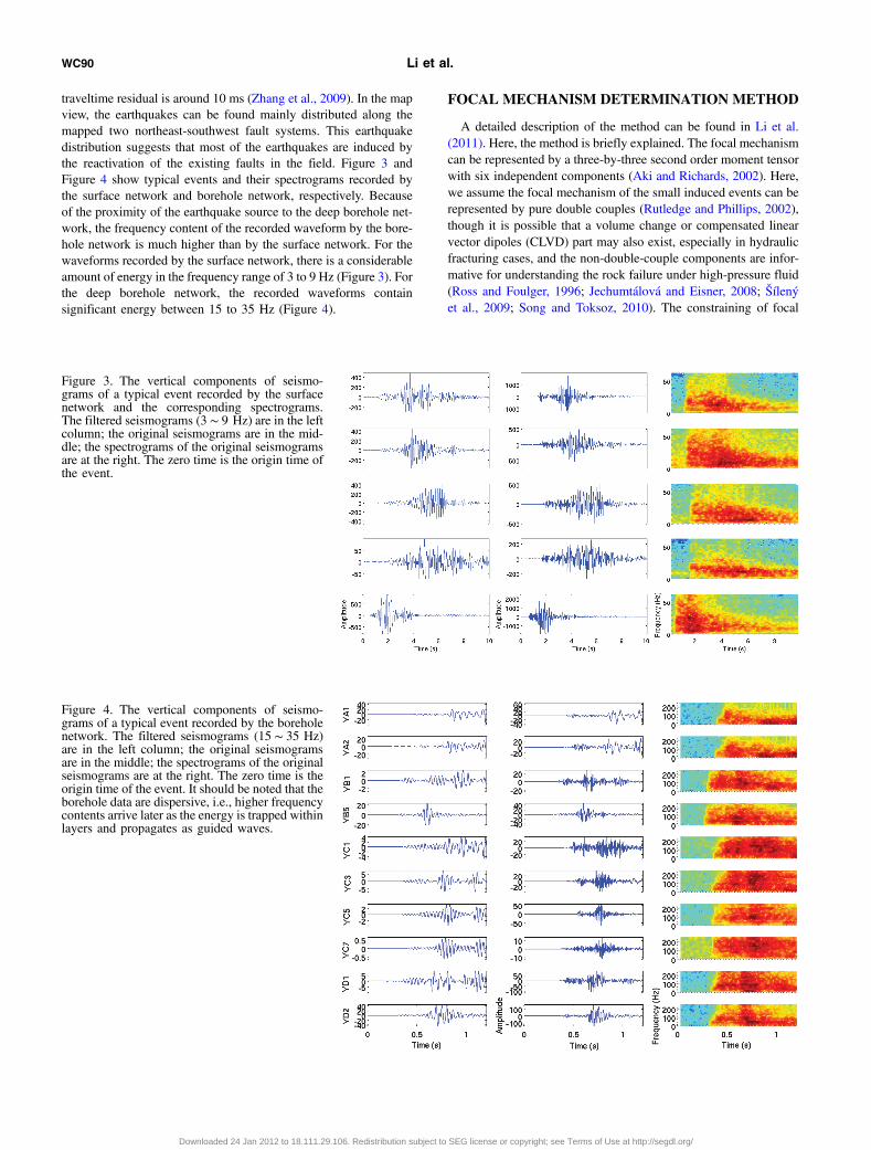
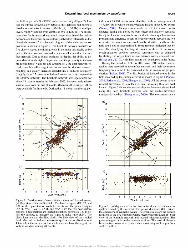
traveltime residual is around 10 ms (Zhang et al., 2009). In the mapview, the earthquakes can be found mainly distributed along themapped two northeast-southwest fault systems. This earthquakedistribution suggests that most of the earthquakes are induced bythe reactivation of the existing faults in the field. Figure 3 andFigure 4 show typical events and their spectrograms recorded bythe surface network and borehole network, respectively. Becauseof the proximity of the earthquake source to the deep borehole net-work, the frequency content of the recorded waveform by the bore-hole network is much higher than by the surface network. For thewaveforms recorded by the surface network, there is a considerableamount of energy in the frequency range of 3 to 9 Hz (Figure 3). Forthe deep borehole network, the recorded waveforms containsignificant energy between 15 to 35 Hz (Figure 4).

FOCAL MECHANISM DETERMINATION METHOD

A detailed description of the method can be found in Li et al.(2011). Here, the method is briefly explained. The focal mechanismcan be represented by a three-by-three second order moment tensorwith six independent components (Aki and Richards, 2002). Here,we assume the focal mechanism of the small induced events can berepresented by pure double couples (Rutledge and Phillips, 2002),though it is possible that a volume change or compensated linearvector dipoles (CLVD) part may also exist, especially in hydraulicfracturing cases, and the non-double-couple components are infor-mative for understanding the rock failure under high-pressure fluid(Ross and Foulger, 1996; Jechumtálová and Eisner, 2008; Šílenýet al., 2009; Song and Toksoz, 2010). The constraining of focal

Figure 4. The vertical components of seismo-grams of a typical event recorded by the boreholenetwork. The filtered seismograms (15 ∼ 35 Hz)are in the left column; the original seismogramsare in the middle; the spectrograms of the originalseismograms are at the right. The zero time is theorigin time of the event. It should be noted that theborehole data are dispersive, i.e., higher frequencycontents arrive later as the energy is trapped withinlayers and propagates as guided waves.

Figure 3. The vertical components of seismo-grams of a typical event recorded by the surfacenetwork and the corresponding spectrograms.The filtered seismograms (3 ∼ 9 Hz) are in the leftcolumn; the original seismograms are in the mid-dle; the spectrograms of the original seismogramsare at the right. The zero time is the origin time ofthe event.

WC90 Li et al.

Downloaded 24 Jan 2012 to 18.111.29.106. Redistribution subject to SEG license or copyright; see Terms of Use at http://segdl.org/

mechanism as double couple (DC) can eliminate the spurious non-DC components in the inversion raised by modeling the wave pro-pagation in anisotropic medium with isotropic Green’s functions orinaccuracy of the velocity model (Šílený and Vavryčuk, 2002;Godano et al., 2011). However, if strong non-DC components ac-tually exist in the source rupture process, the determined fault planemay be biased (e.g., Jechumtálová and Šílený, 2001, 2005). In ouranalysis, we describe the DC focal mechanism of seismic source interms of its strike (Φ), dip (δ), and rake (λ), and determine doublecouple components from these three parameters. The simplificationof the source is supported by the observation that almost all thedetected microearthquakes occurred along preexisting faults, i.e.,reactivated faults slipping along preexisting weak zones wouldnot cause significant volumetric or CLVD components (Julianet al., 1998). For each component of a moment tensor, we usethe discrete wavenumber method (DWN) (Bouchon, 1981, 2003)to calculate its Green’s functionsGn

ij;kðtÞ for the horizontally layeredmedium. Appendix A gives themodified reflectivity matrix for com-puting the seismograms when the receiver is deeper than the source,such as in the borehole monitoring case. It should be noted that if thefullmoment tensor needs to be determined, e.g., in the hydraulic frac-turing cases, the seismic source should be described with six inde-pendent tensor components, whichwill increase the cost in searchingfor the best solution. The structure between the earthquake and thestation is represented as a 1D horizontally layered medium, whichcan be built from (1) averaging borehole sonic logs across this region,or (2) extracting the velocity structure between the source and thereceiver from the 3D velocity model from double-difference seismictomography for passive seismic events (Zhang et al., 2009).The modeled waveform from a certain combination of strike, dip,

and rake is expressed as a linear combination of weighted Green’sfunctions:

Vni ¼

X3j¼1

X3k¼1

mjkGnij;kðtÞ � sðtÞ; (1)

where Vni is the modeled ith (north, east, or vertical) component at

station n; mjk is the moment tensor component and is determined bythe data from all stations;Gn

ij;kðtÞ is the ith component of the Green’sfunctions for the ðj; kÞ entry at station n, and sðtÞ is the source timefunction. In this study, a smooth ramp is used for sðtÞ, the durationof which can be estimated from the spectra of the recorded seismo-grams (Bouchon, 1981). The source time functions are found to beinsensitive to the waveform fitting, as both the synthetic andobserved seismograms are low-pass filtered before comparisons(Zhao et al., 2006). Using reciprocity by straining Green’s tensorscan improve the efficiency of calculating the Green’s functions,especially when the sources greatly outnumber the stations (Eisnerand Clayton, 2001; Zhao et al., 2006). For instance, only one nu-merical simulation with reciprocity (e.g., finite difference method),by setting a source at a station, is needed to calculate the Green’sfunctions for all six components of the moment tensor between any-where in the field and one component at the station in a 3D hetero-geneous medium.Earthquake locations are usually provided by the traveltime loca-

tion method. However, due to uncertainties in velocity model andarrival times, the seismic event locations may have errors, especiallyin focal depth determined from the surface network. While

matching the modeled and observed waveforms, we also searchfor an improved location ðx; y; zÞ around the catalog location.To determine the best solution, we construct an objective function

that characterizes the similarity between the modeled and observedwaveforms. We use the following objective function, which evalu-ates four different aspects of the waveform information:

maximizeðJðx; y; z;Φ; δ; λ; tsÞÞ ¼XNn¼1

X3j¼1

�α1 maxð ~dnj ⊗ ~vnj Þ − α2k ~dnj − ~vnj k2

þα3f ðpolð ~dnj Þ; polð~vnj ÞÞ þ α4h

�rat

�Sðdnj ÞPðdnj Þ

�; rat

�Sðvnj ÞPðvnj Þ

���.

(2)

Here ~dnj is the normalized data and ~vnj is the normalized modeledwaveform; x, y, and z are the event hypocenter that will be redeter-mined by waveform matching; ts is the time shift that gives thelargest crosscorrelation value between the observed and syntheticseismograms (first term). Because it is difficult to obtain accurateabsolute amplitudes due to site effects in many situations, wenormalize the filtered, observed, and modeled waveforms beforecomparison. The normalization used here is the energy normaliza-tion, such that the energy of the normalized wavetrain within a timewindow adds to unity. Compared to peak amplitude normalization,energy normalization is less affected by site effects, which maycause abnormally large peaks due to focusing and other factors.In a concise form, this normalization can be written as

~dnj ¼dnjffiffiffiffiffiffiffiffiffiffiffiffiffiffiffiffiffiffiffiffiffiR t2

t1 ðdnj Þ2dtq (3)

where t1 and t2 are the boundaries of the time window.The objective function J in equation 2 consists of four terms. α1

through α4 are the weights for each term. Each weight is a positivescalar number and is optimally chosen in a way such that no singleterm will overdominate the objective function. We used α1 ¼ 3,α2 ¼ 3, α3 ¼ 1 and α4 ¼ 0.5 for the synthetic tests and real events.The first term in equation 2 evaluates the maximum crosscorrelationbetween the normalized data ( ~dnj ) and the normalized modeled wa-veforms (~vnj ). From the crosscorrelation, we find the time-shift (ts)to align the modeled waveform with the observed waveform. Thesecond term evaluates the L2 norm of the direct differences betweenthe aligned modeled and observed waveforms (note the minus signof the second term to minimize the amplitude differences). The firsttwo terms are not independent of each other, however, they havedifferent sensitivities at different frequency bands and by combiningthem together the waveform similarity can be better characterized.The third term evaluates whether the polarities of the first P-wavearrivals as observed in the data are consistent with those in the mod-eled waveforms. The pol is a weighted sign function which can befβ;−β; 0g, where β is a weight reflecting our confidence in pickingthe polarities of the first P-wave arrivals in the observed data. Zero(0) means undetermined polarity; f is a function that penalizes thepolarity sign inconsistency in such a way that the polarity consis-tency gives a positive value, while polarity inconsistency gives anegative value. The matching of the first P-wave polarities between

Determining focal mechanism by waveforms WC91

Downloaded 24 Jan 2012 to 18.111.29.106. Redistribution subject to SEG license or copyright; see Terms of Use at http://segdl.org/

modeled and observed waveforms is an important condition fordetermining the focal mechanism, when the polarities can be clearlyidentified. Polarity consistency at some stations can be violated ifthe polarity is not confidently identified (small β) and the other threeterms favor a certain focal mechanism. Therefore, the polarity in-formation is integrated into our objective function in a flexible way.By summing over the waveforms in a narrow window around thearrival time and checking the sign of the summation, we determinethe polarities robustly for the modeled data. For the observed data,we determine the P-wave polarities manually.The fourth term in the objective function is to evaluate the con-

sistency of the average S/P amplitude ratios in the observed andmodeled waveforms (Hardebeck & Shearer, 2003). The “rat” isthe ratio evaluation function and it can be written as

rat ¼R T3

T2jrnj ðtÞjdtR T2

T1jrnj ðtÞjdt

; (4)

where ½T1 T2� and ½T2 T3� define the time window of P- andS-waves, respectively, and rnj denotes either dnj or vnj . The term his a function that penalizes the ratio differences so that the bettermatching gives a higher value. Note that here we use the unnorma-lized waveforms dnj and vnj .In general, the amplitudes of P-waves are much smaller than

those of S-waves. To balance the contribution between P- andS-waves, we need to fit P- and S-waves separately using the firsttwo terms in equation 2. Also, by separating S- from P-wavesand allowing an independent time-shift in comparing observed datawith modeled waveforms, it is helpful to deal with incorrect phasearrival time due to incorrect VP∕VS ratios (Zhu and Helmberger,1996). Here, we allow independent shifts for different stations aswell as for P- and S-waves. We calculate both the first P- andS-arrival times by the finite difference eikonal solver (Podvinand Lecomte, 1991). The wavetrain is then separated into two partsat the beginning of the S-wave. The window for the P-wave com-parison is from the first arrival to the beginning of the S-wave, andthe window for the S-wave comparison is proportional to theepicenter distance. It should be noted that the full wavetrain isnot included as later arrivals, usually due to scattering from hetero-geneous media, cause larger inaccuracies in waveform modeling.In some cases, when we have more confidence in some stations,

e.g., stations with short epicenter distance, or stations deployed onknown simpler velocity structure, we can give more weight to thosestations by multiplying α1-α4 with an additional station weightfactor.The comparison algorithm (equation 2) is optimized such that it

can be performed on a multicore desktop machine usually within 30minutes, even when tens of millions of synthetic traces are com-pared with the data. The computation of the Green’s function libraryusing DWN takes more time, but it only needs to be computed once.The passive seismic tomography only provides a detailed 3D ve-

locity model close to the central area of the field due to the earth-quake-station geometry (Zhang et al., 2009). Therefore, for thefocal mechanism determination through the surface network, ofwhich most stations are not placed within the central area (Figure 1),we use the 1D layered velocity model from the averaged sonic logs(Sarkar, 2008; Zhang et al., 2009). Considering that we use a fre-quency band of 3–9 Hz (Figure 3) in our waveform matchingfor this surface network, corresponding to a dominant P-wave

wavelength of 800 m and S-wave wavelength of 400 m, the velocitymodel should satisfy our modeling requirement. The deep networkconsists of five boreholes with eight levels of receivers at differentdepths in each borehole (Figure 2). Due to the proximity of boreholereceivers to the seismicity, we were able to record the seismogramsof very small induced seismicity. Waveforms between 15 and 35 Hzare used to determine the focal mechanisms (Figure 4). To bettermodel the waveforms, we replaced part of the 1D average layeredvelocity model with the extracted P- and S-wave velocities from the3D tomographic model between 0.7 km and 1.2 km in depth, whereit has the highest resolution and reliability. Note that the updated 1Dvelocity model between the earthquake and each station becomesdifferent for the deep borehole network.

SYNTHETIC TESTS FOR THE SURFACEAND DEEP BOREHOLE NETWORKS

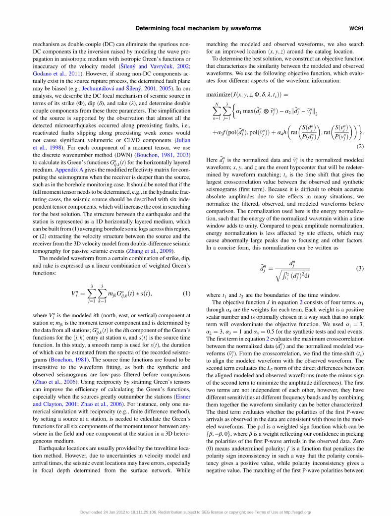
In Li et al. (2011), we tested the robustness of the method on thesurface network. To account for the uncertainty of the 1D velocitymodel, a 5% random perturbation was applied. Here, we consider agreater uncertainty in the velocity model — up to 8% — and testmore cases for different focal mechanisms and event locations. Wefirst use the station configuration of the surface network in our testbecause it provides a considerable challenge due to the large epi-center distance and the relative inaccuracy in the computation ofGreen’s functions by using the 1D averaged velocity model fromseveral sonic logs. We choose three different epicenters (E1, E2, andE3), and for each epicenter we choose three different depths(D1 ¼ 1000 m, D2 ¼ 1200 m, and D3 ¼ 1700 m), correspondingto shallow, medium, and deep events in this field, respectively. Ateach depth, we test three different focal mechanisms, which yield 27different synthetic tests in total. The different focal mechanisms andwidely distributed hypocenters in the synthetic test give a compre-hensive robustness test for the focal mechanism determination inthis region. The station configuration and the hypocenter distribu-tion are shown in Figure 1. At each hypocenter, three distinct me-chanisms are tested, namely M1: Φ ¼ 210°, δ ¼ 50°, λ ¼ −40°;M2: Φ ¼ 50°, δ ¼ 60°, λ ¼ −70°; and M3: Φ ¼ 130°, δ ¼ 80°, λ ¼80° (Table 1). Three or four first P-arrival polarities are used in eachsynthetic test, resembling the measurements we have for real datafor this surface network. In real cases, as inevitable differences existbetween the derived velocity model and the true velocity model, weneed to examine the robustness of our method under such circum-stances. We add up to 8% of the layer’s velocity as the random ve-locity perturbation to the reference velocity model in each layer(Figure 5) and use the perturbed velocity models to generate syn-thetic data. The perturbation is independent for five stations, i.e., thevelocity model is path-dependent and varies among different event-station pairs to reflect the 3D velocity heterogeneities in the field.Also, the perturbation is independent for the P-wave and S-wavevelocities in a specific velocity model for an event-station pair.The Green’s functions (modeled data) are generated with the refer-ence velocity model. Figure 6 shows the modeled seismograms withoffset using the reference velocity model. The predicted traveltimesby the eikonal equation and the first arrivals in the waveforms arematched well. It should also be noted that the P-wave and S-wavevelocity perturbation from one station to another can reach up to800 m/s in some layers. Considering that this reservoir consistsmainly of sedimentary rocks, the magnitude of the random lateralvelocity perturbation should reflect the upper bounds of the local

WC92 Li et al.

Downloaded 24 Jan 2012 to 18.111.29.106. Redistribution subject to SEG license or copyright; see Terms of Use at http://segdl.org/

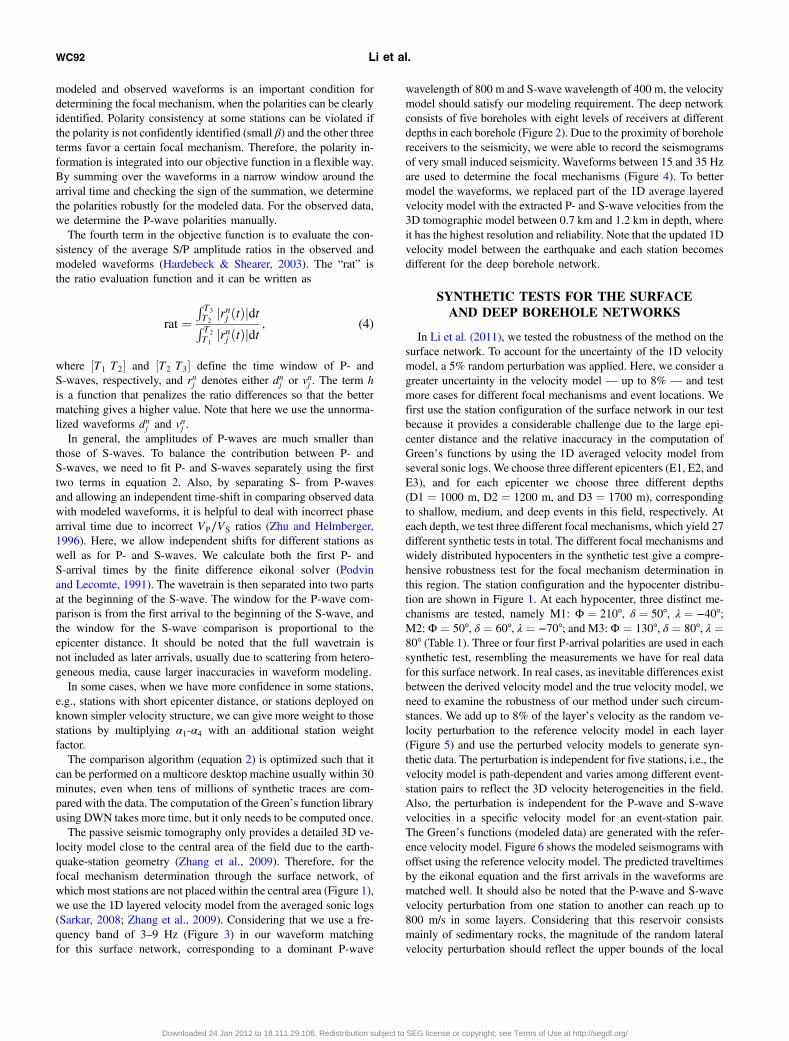
lateral velocity inhomogeneity. The density is not perturbed in thistest, as the velocity perturbation is dominant in determining thecharacteristics of the waveforms. The test results are summarizedin Table 1. Although the perturbation can change the waveformcharacteristics to a very large extent, the synthetic test shows thatour method can still find a solution very close to the correct one byincluding information from different aspects of the waveforms, evenwhen only records from five vertical components are used. Figure 7shows a waveform match between the synthetic data and the mod-eled data. The best solution found is (230°, 60°, −40°), close to thecorrect solution (210°, 50°, −40°) in comparison. The syntheticevent is at 1220 m in depth.In general, the focal mechanisms are reliably recovered (Table 1).

To quantify the recoverability, we define the mean recovery error forthe focal parameters:

Δφem ¼

P3d¼1 jφe

m;d − φmj3

; (7)

where φem;d is the recovered strike, dip, or rake for epicenter e, with

mechanism m at depth d, where e;m; d ∈ f1; 2; 3g, and φm is thereference (true) focal parameter for mechanism m. It is found thatΔφ is only a weak function of epicenter, with marginally smaller

Table 1. Recovered focal mechanisms in the synthetic tests for different hypocenters and faulting types. The true focalmechanisms are listed in the row indicated by REF. Rows D1, D2, and D3 list the events at 1000 m, 1200 m, and 1700 m indepth, respectively.

Figure 5. P- (right) and S-wave (left) velocity perturbations for thesynthetic tests. The reference velocities, plotted with the bold blackline, are used for calculating the Green’s functions. The perturbedvelocities (colored lines) are used to generate the synthetic data foreach station.

Determining focal mechanism by waveforms WC93

Downloaded 24 Jan 2012 to 18.111.29.106. Redistribution subject to SEG license or copyright; see Terms of Use at http://segdl.org/

value for E1 than for E2 or E3, in general. Also, we found that foreach individual depth Δφ (d ¼ 1, 2, or 3) is marginally smaller forshallower earthquakes (D1 and D2) than for deeper earthquakes(D3) (results not tabulated). Due to our use of only vertical com-ponents, we found that the uncertainty in strike is slightly largerthan that in dip or rake. In general, no distinct variation of Δφis found against the hypocenter or faulting type. Therefore, we con-clude that our method is not very sensitive to the faulting type, to theazimuthal coverage of the stations, or to the hypocenter positionwithin a reasonable range for the array geometries studied.For the borehole network, we perform a similar synthetic test to

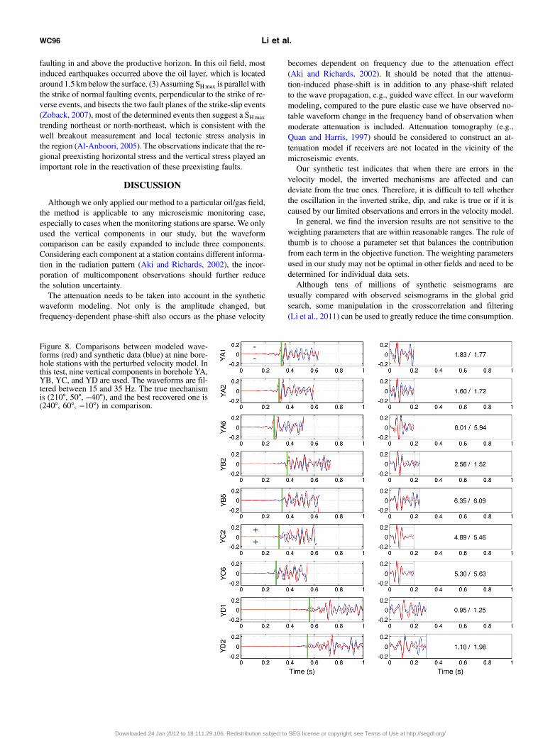
check the reliability of our method for the deep network configura-tion. As we have shown that the reliability of our method is not verysensitive to the azimuthal coverage of the stations or to the depthof the event in a reasonable range, we only perform syntheticexperiments at two hypocenters with three different mechanisms,respectively, for the deep borehole network (Table 2). Nine toeleven receivers are used for each case. The frequency band isthe same as we used for the real data set (15–35 Hz). A typicalwaveform comparison for the synthetic test is shown in Figure 8.It is also found that the method is robust with the borehole receiverconfiguration using higher frequency seismograms.

APPLICATION TO FIELD DATA

We applied this method to study 40 microearthquakes usingsurface and deep borehole networks. The instrumental responseshave been removed before processing. An attenuation model withQ value increasing with depth (Table 3) was used for the waveform

Figure 7. Comparisons between modeled wave-forms (red) and synthetic data (blue) at five sta-tions with perturbed velocity model. From topto bottom, waveforms from the vertical compo-nents at stations one through five, respectively,are shown. The waveforms are filtered between3 and 9 Hz. The left column shows P-wavesand right column shows S-waves. The green linesindicate the first P-arrival times. For P-waves, zerotime means the origin time, and for S-waves, zerotime means the S-wave arrival time predicted bythe calculated traveltime. The “shift” in the titleof each subplot indicates the time shifted in thedata to align with the synthetic waveforms. Inthe left column, the þ or − signs indicate thefirst-arrival polarities of P-waves in the syntheticdata and those in the modeled data, respectively. Inthe right column, the number to the left of the slashdenotes the S/P amplitude ratio for the syntheticdata, and the number to the right of the slash de-notes the ratio for the modeled waveform.

Figure 6. Moveouts of the P- and S-waves with distance. Thesource is at 900-m depth, and the receivers (vertical components)are at 150-m depth. The green lines indicate the first P- andS-wave arrivals obtained from finite-difference traveltime calcula-tion method based on the eikonal equation.

WC94 Li et al.

Downloaded 24 Jan 2012 to 18.111.29.106. Redistribution subject to SEG license or copyright; see Terms of Use at http://segdl.org/

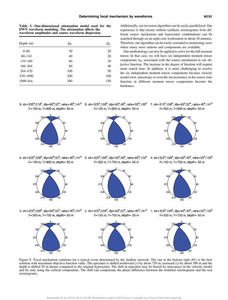
modeling. In general, we consider the attenuation larger (smaller Q)close to the surface due to weathering, and the attenuation forS-waves larger than for P-waves at the same depth. The attenuationmodel is built from empirical knowledge of the local geology, andwe also tested that reasonable deviation from our Q model (50%)causes only small changes in our synthetic waveforms. Figure 9shows the beachballs of the nine best solutions out of millionsof trials for a typical event recorded by the surface network. Ourbest solution (the one at the bottom right, reverse strike-slip) hasa strike of 325°, which is quite close to the best known orientation320° of the northwest-southeast conjugate fault (Figure 1). Figure 10shows the comparison between the modeled and the observed datafor this event. The waveform similarity between the modeled andobserved data is good. Typically, the crosscorrelation coefficient isgreater than 0.7. Additionally, the S/P waveform amplitude ratios inthe modeled and observed data are quite close, and the first P arrivalpolarities are identical in the modeled and observed data for eachstation. In this example, all four criteria in equation 2 are evaluated,and they are consistent between the modeled and observed data.For the deep borehole network, we use the frequency band

15 ∼ 35 Hz, which includes enough energy in the spectra to providegood S/N, for determining the focal mechanisms of these smallmagnitude earthquakes from the borehole network data (Figure 4).The lower frequency here is limited by the bandwidth of the bore-hole instrumentation (f c ¼ 20 Hz), and the frequency contentsbelow the corner frequency f c may suffer from an increased noiselevel. As there is also uncertainty in the orientations of the horizon-tal components, we use only the vertical components of the 4C sen-sors configured in a proprietary tetrahedral shape for each level(Jones et al., 2004). Although there are, in total 40, vertical recei-vers, we often only use about 10 seismograms in determining eachevent due to the following reasons:

• Some receivers are only separated by ∼30 m vertically andtherefore do not provide much additional information for deter-mining the source mechanism.

• Some traces show peculiar, unexplainable characteristics in seis-mograms and are, therefore, discarded. The S/N for some tracesis also very poor.

In our selection of seismograms, we try to in-clude data from different wells to provide a betterazimuthal coverage, as well as from differentdepths spanning a large vertical range, providingwaveform samplings at various radiation direc-tions of the source.Figure 11 shows the comparison between the

observed and modeled seismograms for a typicalevent recorded by the deep borehole network.Eleven receivers from four boreholes are used inthis determination. Among the eleven seismo-grams, five first P-wave arrival polarities areidentified and then used in this determination.The waveform similarities, average S/P ampli-tude ratio, and consistency in the P-wave arrivalpolarities are satisfactory. Comparing Figure 11with Figure 10, we found the fewer matchedcycles in the deep borehole case. Similar compar-ison can also be found between the shallow anddeep borehole synthetic tests (Figures 7 and 8),

where focal mechanisms close to the correct solutions were stillfound in both synthetic cases.Using this method, we have studied 40 earthquakes distributed

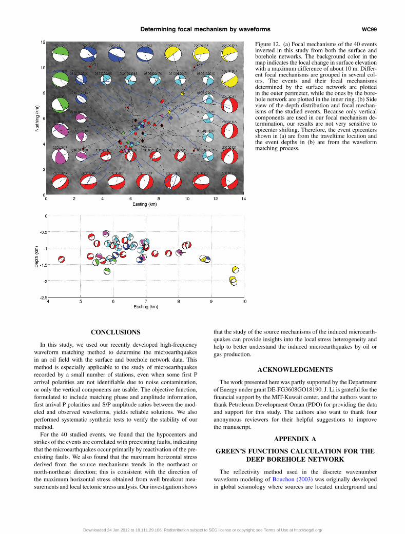
across this oil field from both the surface network and the boreholenetwork. Among these studied events, 22 events are recorded by thesurface network, 18 events are from the borehole network. Figure 12shows that most of the events primarily have the normal faultingmechanism, some have the strike-slip mechanism, and some havea reverse faulting mechanism. The strike directions of most eventsare found to be approximately parallel with the northeast trendingfault, suggesting the correlation of these events with the northeasttrending fault. However, some events also have their strikes in thedirection of the conjugate northwest trending fault, suggesting thatthe reactivation also occurred on the conjugate faults. Although thenumber of studied events is small compared to the total recordedevents, their mechanisms still provide us with some insights onthe fault reactivation in this field: (1) The hypocenter distributionand the determined source mechanisms (e.g., strikes) indicate thatthe reactivation of preexisting faults is the main cause of the inducedmicroearthquakes in this field, and both the northeast trending faultand its conjugate fault trending in the northwest direction are stillactive. Interestingly, we note that the strike directions of the normalfaulting events (red) are slightly rotated counterclockwise with re-spect to the mapped fault traces from the 3D active seismic data andare consistent with the trend of the located earthquake locations(Figure 1). (2) The counterclockwise rotation may be due to thenonplanar geometry of the fault, i.e., the strike of the shallow partof the fault as delineated by the surface seismic survey does notneed to be the same as the deeper part of the fault, where most in-duced seismicity is located. Most strike-slip events (cyan) areshallow, suggesting that the maximum horizontal stress (SHmax)is still larger than the vertical stress (SV) at this depth range. How-ever, deeper events (e.g., red, blue) mainly have a normal faultingmechanism, suggesting SV exceeds SHmax when depth increases be-yond ∼1 km in this region. The dominance of normal faulting isconsistent with the study by Zoback and Zinke (2002) on the Valhalland Ekofisk oil fields, where reservoir depletion induced normal

Table 2. Recovered focal mechanisms in the synthetic tests for different faultingtypes using the deep borehole network. The true focal mechanisms are listed inthe row indicated by REF. The synthetic events at two different hypocentersare tested (Figure 2).

Determining focal mechanism by waveforms WC95

Downloaded 24 Jan 2012 to 18.111.29.106. Redistribution subject to SEG license or copyright; see Terms of Use at http://segdl.org/

faulting in and above the productive horizon. In this oil field, mostinduced earthquakes occurred above the oil layer, which is locatedaround 1.5 kmbelow the surface. (3)AssumingSHmax is parallel withthe strike of normal faulting events, perpendicular to the strike of re-verse events, and bisects the two fault planes of the strike-slip events(Zoback, 2007), most of the determined events then suggest a SHmax

trending northeast or north-northeast, which is consistent with thewell breakout measurement and local tectonic stress analysis inthe region (Al-Anboori, 2005). The observations indicate that the re-gional preexisting horizontal stress and the vertical stress played animportant role in the reactivation of these preexisting faults.

DISCUSSION

Although we only applied our method to a particular oil/gas field,the method is applicable to any microseismic monitoring case,especially to cases when the monitoring stations are sparse. We onlyused the vertical components in our study, but the waveformcomparison can be easily expanded to include three components.Considering each component at a station contains different informa-tion in the radiation pattern (Aki and Richards, 2002), the incor-poration of multicomponent observations should further reducethe solution uncertainty.The attenuation needs to be taken into account in the synthetic

waveform modeling. Not only is the amplitude changed, butfrequency-dependent phase-shift also occurs as the phase velocity

becomes dependent on frequency due to the attenuation effect(Aki and Richards, 2002). It should be noted that the attenua-tion-induced phase-shift is in addition to any phase-shift relatedto the wave propagation, e.g., guided wave effect. In our waveformmodeling, compared to the pure elastic case we have observed no-table waveform change in the frequency band of observation whenmoderate attenuation is included. Attenuation tomography (e.g.,Quan and Harris, 1997) should be considered to construct an at-tenuation model if receivers are not located in the vicinity of themicroseismic events.Our synthetic test indicates that when there are errors in the

velocity model, the inverted mechanisms are affected and candeviate from the true ones. Therefore, it is difficult to tell whetherthe oscillation in the inverted strike, dip, and rake is true or if it iscaused by our limited observations and errors in the velocity model.In general, we find the inversion results are not sensitive to the

weighting parameters that are within reasonable ranges. The rule ofthumb is to choose a parameter set that balances the contributionfrom each term in the objective function. The weighting parametersused in our study may not be optimal in other fields and need to bedetermined for individual data sets.Although tens of millions of synthetic seismograms are

usually compared with observed seismograms in the global gridsearch, some manipulation in the crosscorrelation and filtering(Li et al., 2011) can be used to greatly reduce the time consumption.

Figure 8. Comparisons between modeled wave-forms (red) and synthetic data (blue) at nine bore-hole stations with the perturbed velocity model. Inthis test, nine vertical components in borehole YA,YB, YC, and YD are used. The waveforms are fil-tered between 15 and 35 Hz. The true mechanismis (210°, 50°, −40°), and the best recovered one is(240°, 60°, −10°) in comparison.

WC96 Li et al.

Downloaded 24 Jan 2012 to 18.111.29.106. Redistribution subject to SEG license or copyright; see Terms of Use at http://segdl.org/

Additionally, our inversion algorithm can be easily parallelized. Ourexperience is that twenty million synthetic seismograms from dif-ferent source mechanism and hypocenter combinations can besearched through on an eight-core workstation in about 20 minutes.Therefore, our algorithm can be easily extended to monitoring caseswhere many more stations and components are available.Our methodology can also be applied to solve for the full moment

tensor. In that case, we will have six independent moment tensorcomponents mjk associated with the source mechanism in our ob-jective function. The increase in the degree of freedom will requiremore search time. In addition, it is more challenging to resolvethe six independent moment tensor components because velocitymodel error, anisotropy or even the inconsistency in the source timefunction in different moment tensor components become thehindrance.

Figure 9. Focal mechanism solutions for a typical event determined by the shallow network. The one at the bottom right (#1) is the bestsolution with maximum objective function value. The epicenter is shifted northward (y) by about 750 m, eastward (x) by about 300 m and thedepth is shifted 50 m deeper compared to the original hypocenter. The shift in epicenter may be biased by inaccuracy in the velocity modeland by only using the vertical components. The shift can compensate the phase difference between the modeled seismograms and the realseismograms.

Table 3. One-dimensional attenuation model used for theDWN waveform modeling. The attenuation affects thewaveform amplitudes and causes waveform dispersion.

Depth (m) QP QS

0–60 30 20

60–110 40 20

110–160 60 30

160–264 80 40

264–470 100 50

470–1090 200 100

1090–bot. 300 150

Determining focal mechanism by waveforms WC97

Downloaded 24 Jan 2012 to 18.111.29.106. Redistribution subject to SEG license or copyright; see Terms of Use at http://segdl.org/

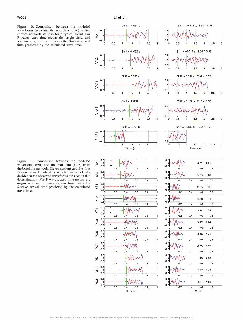
Figure 10. Comparison between the modeledwaveforms (red) and the real data (blue) at fivesurface network stations for a typical event. ForP-waves, zero time means the origin time, andfor S-waves, zero time means the S-wave arrivaltime predicted by the calculated traveltime.

Figure 11. Comparison between the modeledwaveforms (red) and the real data (blue) fromthe borehole network. Eleven stations and five firstP-wave arrival polarities which can be clearlydecided in the observed waveforms are used in thisdetermination. For P-waves, zero time means theorigin time, and for S-waves, zero time means theS-wave arrival time predicted by the calculatedtraveltime.

WC98 Li et al.

Downloaded 24 Jan 2012 to 18.111.29.106. Redistribution subject to SEG license or copyright; see Terms of Use at http://segdl.org/

CONCLUSIONS

In this study, we used our recently developed high-frequencywaveform matching method to determine the microearthquakesin an oil field with the surface and borehole network data. Thismethod is especially applicable to the study of microearthquakesrecorded by a small number of stations, even when some first Parrival polarities are not identifiable due to noise contamination,or only the vertical components are usable. The objective function,formulated to include matching phase and amplitude information,first arrival P polarities and S/P amplitude ratios between the mod-eled and observed waveforms, yields reliable solutions. We alsoperformed systematic synthetic tests to verify the stability of ourmethod.For the 40 studied events, we found that the hypocenters and

strikes of the events are correlated with preexisting faults, indicatingthat the microearthquakes occur primarily by reactivation of the pre-existing faults. We also found that the maximum horizontal stressderived from the source mechanisms trends in the northeast ornorth-northeast direction; this is consistent with the direction ofthe maximum horizontal stress obtained from well breakout mea-surements and local tectonic stress analysis. Our investigation shows

that the study of the source mechanisms of the induced microearth-quakes can provide insights into the local stress heterogeneity andhelp to better understand the induced microearthquakes by oil orgas production.

ACKNOWLEDGMENTS

The work presented here was partly supported by the Departmentof Energy under grant DE-FG3608GO18190. J. Li is grateful for thefinancial support by the MIT-Kuwait center, and the authors want tothank Petroleum Development Oman (PDO) for providing the dataand support for this study. The authors also want to thank fouranonymous reviewers for their helpful suggestions to improvethe manuscript.

APPENDIX A

GREEN’S FUNCTIONS CALCULATION FOR THEDEEP BOREHOLE NETWORK

The reflectivity method used in the discrete wavenumberwaveform modeling of Bouchon (2003) was originally developedin global seismology where sources are located underground and

Figure 12. (a) Focal mechanisms of the 40 eventsinverted in this study from both the surface andborehole networks. The background color in themap indicates the local change in surface elevationwith a maximum difference of about 10 m. Differ-ent focal mechanisms are grouped in several col-ors. The events and their focal mechanismsdetermined by the surface network are plottedin the outer perimeter, while the ones by the bore-hole network are plotted in the inner ring. (b) Sideview of the depth distribution and focal mechan-isms of the studied events. Because only verticalcomponents are used in our focal mechanism de-termination, our results are not very sensitive toepicenter shifting. Therefore, the event epicentersshown in (a) are from the traveltime location andthe event depths in (b) are from the waveformmatching process.

Determining focal mechanism by waveforms WC99

Downloaded 24 Jan 2012 to 18.111.29.106. Redistribution subject to SEG license or copyright; see Terms of Use at http://segdl.org/

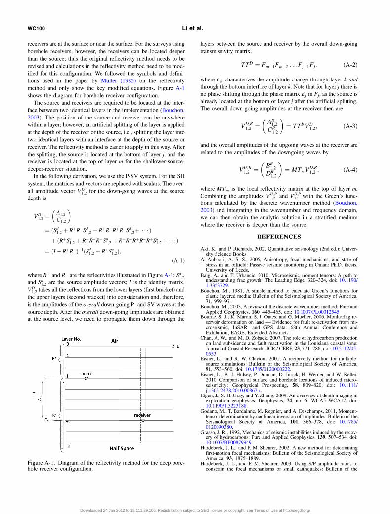
receivers are at the surface or near the surface. For the surveys usingborehole receivers, however, the receivers can be located deeperthan the source; thus the original reflectivity method needs to berevised and calculations in the reflectivity method need to be mod-ified for this configuration. We followed the symbols and defini-tions used in the paper by Muller (1985) on the reflectivitymethod and only show the key modified equations. Figure A-1shows the diagram for borehole receiver configuration.The source and receivers are required to be located at the inter-

face between two identical layers in the implementation (Bouchon,2003). The position of the source and receiver can be anywherewithin a layer; however, an artificial splitting of the layer is appliedat the depth of the receiver or the source, i.e., splitting the layer intotwo identical layers with an interface at the depth of the source orreceiver. The reflectivity method is easier to apply in this way. Afterthe splitting, the source is located at the bottom of layer j, and thereceiver is located at the top of layer m for the shallower-source-deeper-receiver situation.In the following derivation, we use the P-SV system. For the SH

system, the matrices and vectors are replaced with scalars. The over-all amplitude vector VD

1;2 for the down-going waves at the sourcedepth is

VD1;2 ¼

�A1;2

C1;2

�

¼ ðSd1;2 þ RþR−Sd1;2 þ RþR−RþR−Sd1;2þ · · · Þþ ðRþSu1;2 þ RþR−RþSu1;2 þ RþR−RþR−RþSu1;2þ · · · Þ

¼ ðI − RþR−Þ−1ðSd1;2 þ RþSu1;2Þ;(A-1)

where Rþ and R− are the reflectivities illustrated in Figure A-1; Sd1;2and Su1;2 are the source amplitude vectors; I is the identity matrix.VD1;2 takes all the reflections from the lower layers (first bracket) and

the upper layers (second bracket) into consideration and, therefore,is the amplitudes of the overall down-going P- and SV-waves at thesource depth. After the overall down-going amplitudes are obtainedat the source level, we need to propagate them down through the

layers between the source and receiver by the overall down-goingtransmissivity matrix,

TTD ¼ Fm−1Fm−2 : : :Fjþ1Fj; (A-2)

where Fk characterizes the amplitude change through layer k andthrough the bottom interface of layer k. Note that for layer j there isno phase shifting through the phase matrix Ej in Fj, as the source isalready located at the bottom of layer j after the artificial splitting.The overall down-going amplitudes at the receiver then are

VD;R1;2 ¼

�AR1;2

CR1;2

�¼ TTDVD

1;2; (A-3)

and the overall amplitudes of the upgoing waves at the receiver arerelated to the amplitudes of the downgoing waves by

VU;R1;2 ¼

�BR1;2

DR1;2

�¼ MTmV

D;R1;2 ; (A-4)

where MTm is the local reflectivity matrix at the top of layer m.Combining the amplitudes VU;R

1;2 and VD;R1;2 with the Green’s func-

tions calculated by the discrete wavenumber method (Bouchon,2003) and integrating in the wavenumber and frequency domain,we can then obtain the analytic solution in a stratified mediumwhere the receiver is deeper than the source.

REFERENCES

Aki, K., and P. Richards, 2002, Quantitative seismology (2nd ed.): Univer-sity Science Books.

Al-Anboori, A. S. S., 2005, Anisotropy, focal mechanisms, and state ofstress in an oilfield: Passive seismic monitoring in Oman: Ph.D. thesis,University of Leeds.

Baig, A., and T. Urbancic, 2010, Microseismic moment tensors: A path tounderstanding frac growth: The Leading Edge, 320–324, doi: 10.1190/1.3353729.

Bouchon, M., 1981, A simple method to calculate Green’s functions forelastic layered media: Bulletin of the Seismological Society of America,71, 959–971.

Bouchon, M., 2003, A review of the discrete wavenumber method: Pure andApplied Geophysics, 160, 445–465, doi: 10.1007/PL00012545.

Bourne, S. J., K. Maron, S. J. Oates, and G. Mueller, 2006, Monitoring re-servoir deformation on land — Evidence for fault re-activation from mi-croseismic, InSAR, and GPS data: 68th Annual Conference andExhibition, EAGE, Extended Abstracts.

Chan, A. W., and M. D. Zoback, 2007, The role of hydrocarbon productionon land subsidence and fault reactivation in the Louisiana coastal zone:Journal of Coastal Research: JCR / CERF, 23, 771–786, doi: 10.2112/05-0553.

Eisner, L., and R. W. Clayton, 2001, A reciprocity method for multiple-source simulations: Bulletin of the Seismological Society of America,91, 553–560, doi: 10.1785/0120000222.

Eisner, L., B. J. Hulsey, P. Duncan, D. Jurick, H. Werner, and W. Keller,2010, Comparison of surface and borehole locations of induced micro-seismicity: Geophysical Prospecting, 58, 809–820, doi: 10.1111/j.1365-2478.2010.00867.x.

Etgen, J., S. H. Gray, and Y. Zhang, 2009, An overview of depth imaging inexploration geophysics: Geophysics, 74, no. 6, WCA5–WCA17, doi:10.1190/1.3223188.

Godano, M., T. Bardainne, M. Regnier, and A. Deschamps, 2011, Moment-tensor determination by nonlinear inversion of amplitudes: Bulletin of theSeismological Society of America, 101, 366–378, doi: 10.1785/0120090380.

Grasso, J. R., 1992, Mechanics of seismic instabilities induced by the recov-ery of hydrocarbons: Pure and Applied Geophysics, 139, 507–534, doi:10.1007/BF00879949.

Hardebeck, J. L., and P. M. Shearer, 2002, A new method for determiningfirst-motion focal mechanisms: Bulletin of the Seismological Society ofAmerica, 93, 1875–1889.

Hardebeck, J. L., and P. M. Shearer, 2003, Using S/P amplitude ratios toconstrain the focal mechanisms of small earthquakes: Bulletin of the

Figure A-1. Diagram of the reflectivity method for the deep bore-hole receiver configuration.

WC100 Li et al.

Downloaded 24 Jan 2012 to 18.111.29.106. Redistribution subject to SEG license or copyright; see Terms of Use at http://segdl.org/

Seismological Society of America, 93, 2434–2444, doi: 10.1785/0120020236.

Jechumtálová, Z., and L. Eisner, 2008, Seismic source mechanism inversionfrom a linear array of receivers reveals non-double-couple seismic eventsinduced by hydraulic fracturing in sedimentary formation: Tectonophy-sics, 460, 124–133, doi: 10.1016/j.tecto.2008.07.011.

Jechumtálová, Z., and J. Šílený, 2001, Point-source parameters from noisywaveforms: Error estimate by Monte Carlo simulation: Pure and AppliedGeophysics, 158, 1639–1654, doi: 10.1007/PL00001237.

Jechumtálová, Z., and J. Šílený, 2005, Amplitude ratios for completemoment tensor retrieval: Geophysical Research Letters, 32, L22303,doi: 10.1029/2005GL023967.

Jones, R. H., D. Raymer, G. Mueller, H. Rynja, and K. Maron, 2004,Microseismic monitoring of the Yibal oilfield: 66th Annual Conferenceand Exhibition, Extended Abstracts.

Julià, J., and A. A. Nyblade, 2009, Source mechanisms of mine-relatedseismicity, Savuka mine, South Africa: Bulletin of the SeismologicalSociety of America, 99, 2801–2814, doi: 10.1785/0120080334.

Julian, B. R., G. R. Foulger, and F. Monastero, 2007, Microearthquakemoment tensors from the Coso geothermal area: Proceedings, Thirty-Second Workshop on Geothermal Reservoir Engineering, PaperSGP-TR-183: Stanford University.

Julian, B. R., A. D. Miller, and G. R. Foulger, 1998, Non-double-coupleearthquakes, 1. Theory: Reviews of Geophysics, 36, 4525–549, doi:10.1029/98RG00716.

Li, J., H. Zhang, H. S. Kuleli, and M. N. Toksoz, 2011, Focal mechanismdetermination using high-frequency waveform matching and its applica-tion to small magnitude induced earthquakes: Geophysical JournalInternational, 184, 1261–1274, doi: 10.1111/gji.2011.184.issue-3.

Maury, V. M. R., J. R. Grasso, and G. Wittlinger, 1992, Monitoring ofsubsidence and induced seismicity in the Larq gas field (France): Theconsequences on gas production and field operation: EngineeringGeology, 32, 123–135, doi: 10.1016/0013-7952(92)90041-V.

Maxwell, S. C., J. Rutledge, R. Jones, and M. Fehler, 2010, Petroleumreservoir characterization using downhole microseismic monitoring:Geophysics, 75, no. 5, 75A129–75A137, doi: 10.1190/1.3477966.

Miyazawa, M., A. Venkataraman, R. Snieder, and M. A. Payne, 2008,Analysis of microearthquake data at Cold Lake and its applications toreservoir monitoring: Geophysics, 73, 3, O15–O21, doi: 10.1190/1.2901199.

Muller, G., 1985, The reflectivity method: A tutorial: Journal of Geophysics,58, 153–174.

Nolen-Hoeksema, R. C., and L. J. Ruff, 2001, Moment tensor inversionof microseisms from the B-sand propped hydrofracture, M-site,Colorado: Tectonophysics, 336, 163–181, doi: 10.1016/S0040-1951(01)00100-7.

Podvin, P., and I. Lecomte, 1991, Finite difference computation of travel-times in very contrasted velocity models: A massively parallel approachand its associated tools: Geophysical Journal International, 105, 271–284,doi: 10.1111/gji.1991.105.issue-1.

Quan, Y., and J. Harris, 1997, Seismic attenuation tomography using thefrequency shift method: Geophysics, 62, 895–905, doi: 10.1190/1.1444197.

Ross, A., and G. R. Foulger, 1996, Non-double-couple earthquake mechan-ism at The Geysers geothermal area, California: Geophysical ResearchLetters, 23, 877–880, doi: 10.1029/96GL00590.

Rutledge, J. T., and W. S. Phillips, 2002, A comparison of microseismicityinduced by gel-proppant and water-injected hydraulic fractures, CarthageCotton Valley gas field, east Texas: 72nd Annual International Meeting,SEG, Expanded Abstracts, 2393–2396.

Sarkar, S., 2008, Reservoir monitoring using induced seismicity at a petro-leum field in Oman: Ph.D. thesis, Massachusetts Institute of Technology.

Sarkar, S., H. S. Kuleli, M. N. Toksoz, H. Zhang, O. Ibi, F. Al-Kindy, and N.Al Touqi, 2008, Eight years of passive seismic monitoring at a petroleumfield in Oman: A case study: 78th Annual International Meeting, SEG,Expended Abstracts, 1397–1401.

Šílený, J., D. P. Hill, L. Eisner, and F. H. Cornet, 2009, Non-double-couplemechanisms of microearthquakes induced by hydraulic fracturing:Journal of Geophysical Research, 114, B08307, doi: 10.1029/2008JB005987.

Šílený, J., G. F. Panza, and P. Campus, 1992, Waveform inversion for pointsource moment tensor retrieval with variable hypocentral depth andstructural model: Geophysical Journal International, 109, 259–274,doi: 10.1111/gji.1992.109.issue-2.

Šílený, J., and V. Vavryčuk, 2002, Can unbiased source be retrieved fromanisotropic waveforms by using an isotropic model of the medium?:Tectonphysics, 356, 1–3, 125–138, doi: 10.1016/S0040-1951(02)00380-3.

Song, F., and M. N. Toksoz, 2010, Downhole microseismic monitoring ofhydraulic fracturing: A full-waveform approach for complete momenttensor inversion and stress estimation: Presented at 2010 SEG micro-seismicity workshop.

Suckale, J., 2010, Chapter 2 — Induced seismicity in hydrocarbon fields:Advances in Geophysics, 51, 55–106, doi: 10.1016/S0065-2687(09)05107-3.

Tan, Y., and D. V. Helmberger, 2007, A new method for determining smallearthquake source parameters using short-period P waves: Bulletin of theSeismological Society of America, 97, 1176–1195, doi: 10.1785/0120060251.

Willson, S., N. C. Last, M. D. Zoback, and D. Moos, 1998, Drilling in SouthAmerica: Awellbore stability approach for complex geologic conditions:SPE 53940, in 1999 SPE Latin American and Caribbean petroleumengineering conference, 1–23.

Zhang, H. J., S. Sarkar, M. N. Toksoz, H. S. Kuleli, and F. Al-Kindy, 2009,Passive seismic tomography using induced seismicity at a petroleum fieldin Oman: Geophysics, 74, no. 6, WCB57–WCB69, doi: 10.1190/1.3253059.

Zhao, L., P. Chen, and T. H. Jordan, 2006, Strain Green’s tensors, reciprocityand their applications to seismic source and structure studies: Bulletin ofthe Seismological Society of America, 96, 1753–1763, doi: 10.1785/0120050253.

Zhao, L. S., and D. V. Helmberger, 1994, Source estimation from broadbandregional seismograms: Bulletin of the Seismological Society of America,84, 91–104.

Zhu, L. P., and D. V. Helmberger, 1996, Advancement in source estimationtechniques using broadband regional seismograms: Bulletin of theSeismological Society of America, 86, 1634–1641.

Zoback, M. D., 2007, Reservoir geomechanics: Cambridge University Press.Zoback, M. D., and J. C. Zinke, 2002, Production-induced normal faultingin the Valhall and Ekofisk oil fields: Pure and Applied Geophysics, 159,403–420, doi: 10.1007/PL00001258.

Determining focal mechanism by waveforms WC101

Downloaded 24 Jan 2012 to 18.111.29.106. Redistribution subject to SEG license or copyright; see Terms of Use at http://segdl.org/