Fluid-Structure Coupling for Aeroelastic Computations in the Time Domain using Low

Fidelity Structural Models

LiangKan Zheng

Master of Engineering

Department of Mechanical Engineering

McGill University

Montreal, Quebec, Canada

2005-10-17

A thesis submitted to McGill University in Partial Fulfillment of the Requirements for the Degree of Master of Engineering

@L.K. Zheng 2005

1+1 Library and Archives Canada

Bibliothèque et Archives Canada

Published Heritage Branch

Direction du Patrimoine de l'édition

395 Wellington Street Ottawa ON K1A ON4 Canada

395, rue Wellington Ottawa ON K1A ON4 Canada

NOTICE: The author has granted a non­exclusive license allowing Library and Archives Canada to reproduce, publish, archive, preserve, conserve, communicate to the public by telecommunication or on the Internet, loan, distribute and sell th es es worldwide, for commercial or non­commercial purposes, in microform, paper, electronic and/or any other formats.

The author retains copyright ownership and moral rights in this thesis. Neither the thesis nor substantial extracts from it may be printed or otherwise reproduced without the author's permission.

ln compliance with the Canadian Privacy Act some supporting forms may have been removed from this thesis.

While these forms may be included in the document page count, their removal does not represent any loss of content from the thesis.

• •• Canada

AVIS:

Your file Votre référence ISBN: 978-0-494-25023-5 Our file Notre référence ISBN: 978-0-494-25023-5

L'auteur a accordé une licence non exclusive permettant à la Bibliothèque et Archives Canada de reproduire, publier, archiver, sauvegarder, conserver, transmettre au public par télécommunication ou par l'Internet, prêter, distribuer et vendre des thèses partout dans le monde, à des fins commerciales ou autres, sur support microforme, papier, électronique et/ou autres formats.

L'auteur conserve la propriété du droit d'auteur et des droits moraux qui protège cette thèse. Ni la thèse ni des extraits substantiels de celle-ci ne doivent être imprimés ou autrement reproduits sans son autorisation.

Conformément à la loi canadienne sur la protection de la vie privée, quelques formulaires secondaires ont été enlevés de cette thèse.

Bien que ces formulaires aient inclus dans la pagination, il n'y aura aucun contenu manquant.

ACKNOWLEDGEMENTS

I would like to express my sincere gratitude to Professor Siva Nadarajah for bis sup­

port and guidance throughout tbis work. He has given me considerable freedom and shown

patience as I pursed the idea development in this project. I would also like to thank Pro­

fessor Wagdi Habishi for bis suggestions for this project. I have enjoyed the encouragement

and warm company of my colleague in the CFD lab at McGill University. Special thanks

to Dr. Claude Lepage and Dr. Remaki Lakhdar for their ideals and helpful technical

discussion. I thank Dr. Kasidit Leoviriyakit for bis encouragement. I also thank my fellow

students for useful discussion with them. Further, I would like to extend my gratitude to

Martin Aubé, Dr. Guido S. Baruzzi, Nabil Ben Abdallah, Hongzhi Wang of Newmerical

Technologies International for their helping with my research. Above all, I thank Ping Li,

my wife and friend, her love and support make my life more beautiful and meaningful.

ii

ABSTRACT

Flutter analysis plays an important role in the design and development of aircraft

wings because of the information it provides regarding the flight envelope of the aircraft.

With the coupling of the flow and structural solver, the flutter boundary of wings can

be evaluated in the time domain. This study: First, computes the aeroelastic response

for a typical sweptback wing section model by coupling a flow solver and a two degree

of freedom structural equation of motion solver to predict the flutter boundary of an

airfoil at different Mach numbers. The results agree well with previous numerical results,

and the transonic-dip phenomenon can be observed. Second, a new coupling approach is

introduced to conservatively transfer the load and displacement between the flow solver

and the structural solver for 3-D flow. By coupling the flow solver and a low fidelity finite

element structural model, the flutter point of AGARD wing 445.6 at Mach number 0.499 is

computed. The Hutter point agrees well with experimental results and previous numerical

results.

iii

RÉSUMÉ

L'analyse d'oscillations joue un rôle important dans le design et le développement

des ailes d'avion puisqu'elle fournit une information précieuse de l'enveloppe de vol de

l'avion. Avec l'agencement des solveurs d'écoulement et de structure, la limite d'oscillation

des ailes peut être évaluée en considérant le temps. Tout d'abord cette étude calcule la

réponse aéroélastique d'un model de section d'aile en flèche positive, en couplant un solveur

d'écoulement et un solveur d'équation de mouvement structurel a deux degrés de liberté,

afin de prédire la limite d'oscillations d'un profile d'aile portante a différents nombres

de Mach. Les résultats concordent bien avec les résultats numériques précédents, et le

phénoméne puit-transsonique peut être observé. Deuxièmement, une nouvelle approche

couplée est introduite afin de transférer avec précaution la charge et le déplacement entre

les solveurs d'écoulement et de structure pour un fluide en trois dimensions. En couplant

le solveur d'écoulement et le modèle structurel à fidélité réduite d'éléments finis, le point

d'oscillation d'une aile AGARD 445.6 a été calculé à nombre de Mach de 0.499. Le point

d'oscillation concorde bien avec les résultats expérimentaux et les résultats numériques

obtenus précédemment.

iv

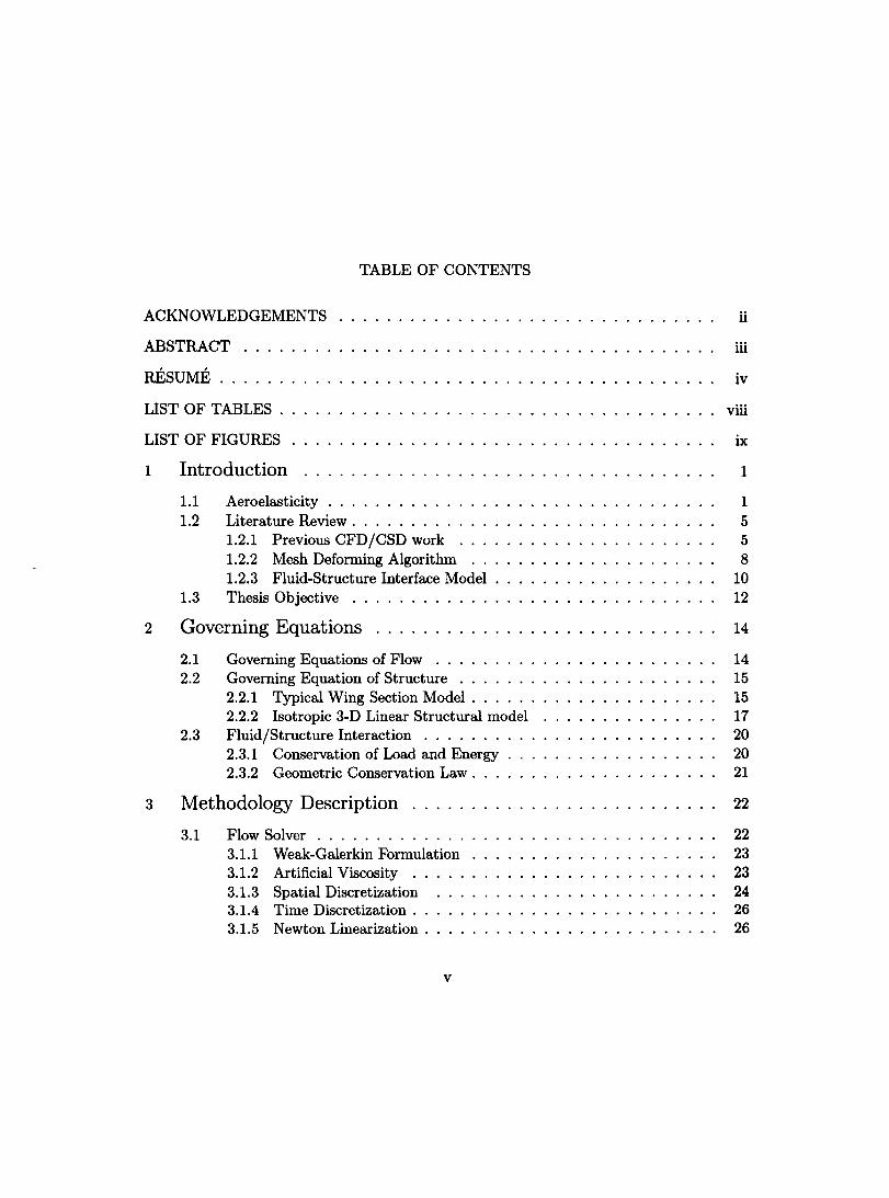
TABLE OF CONTENTS

ACKNOWLEDGEMENTS

ABSTRACT

RÉSUMÉ ..

LIST OF TABLES .

LIST OF FIGURES

1

2

3

Introd uction

1.1 Aeroelasticity 1.2 Literature Review .

1.2.1 Previous CFD/CSD work 1.2.2 Mesh Deforming Aigorithm 1.2.3 Fluid-Structure Interface Model

1.3 Thesis Objective ..

Governing Equations ...... .

2.1 Governing Equations of Flow . . 2.2 Governing Equation of Structure

2.2.1 Typical Wing Section Model . 2.2.2 Isotropic 3-D Linear Structural model

2.3 Fluid/Structure Interaction . . . . . . . 2.3.1 Conservation of LoOO and Energy 2.3.2 Geometrie Conservation Law.

Methodology Description . . ...

3.1 Flow Solver . . . . . . . . . . . . . 3.1.1 Weak-Galerkin Formulation 3.1.2 Artificial Viscosity .. 3.1.3 Spatial Discretization 3.1.4 Time Discretization . . 3.1.5 Newton Linearization .

v

ii

iii

iv

viii

ix

1

1 5 5 8

10 12

14

14 15 15 17 20 20 21

22

22 23 23 24 26 26

3.1.6 Time-Marching approach . . 27 3.1.7 Boundary Conditions . . . . 27 3.1.8 Mesh Deforming Aigorithm 28

3.2 Structural Mechanics . . . . . . . . 28 3.2.1 Finite Element Analysis of Structure 30 3.2.2 Time Integration Approach 32 3.2.3 Finite Element Model. . 33 3.2.4 Damping Characteristics 34

3.3 Fluid-Structure Interface . . . 35 3.3.1 Displacement Transfer 36 3.3.2 Load Transfer . . . . 39 3.3.3 Coupling Procedure. 39

4 Isogai Test Case . . 45

4.1 Physical Model 45 4.2 Mesh Generation 46 4.3 Numerical Setup 46 4.4 Results ...... 47

4.4.1 Initial solution . 47 4.4.2 Pitching Airfoil 49 4.4.3 Aeroelastic Simulation 52 4.4.4 Effect of High-density Region 64 4.4.5 Effect of Coupling Time Step 67 4.4.6 Effect of Number of Sub-Iterations 67

5 Sweptback Wing Test Case . 71

5.1 Physical Model .. 71 5.2 Mesh Generation 73

5.2.1 Fluid Mesh 73 5.2.2 Structural Mesh . 74

5.3 N umerical Setup ... 77 5.4 Results .......... 81

5.4.1 Initial solution. . 81 5.4.2 Aeroelastic computation 83 5.4.3 Effects of Coupling ... 84 5.4.4 Effect of Artificial Viscosity 84

6 Conclusions ... 86

6.1 Future Work 87

vi

R.eferences. . . . . . . . . . . . . . . . . . . . . . . . . . . . . . . . . . . . . . . . .. 89

vii

LIST OF TABLES Table

5-1 Comparison of Natural Frequencies ..... .

viii

~

72

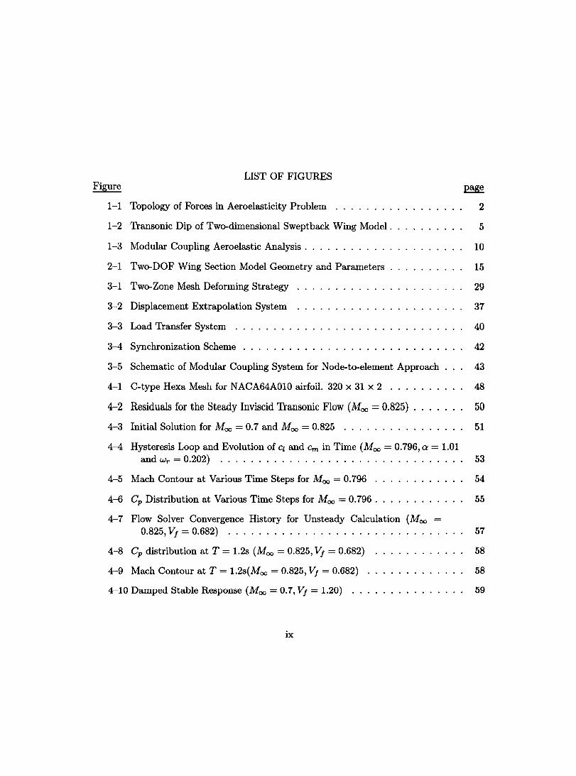
LIST OF FIGURES Figure

1-1 Topology of Forces in Aeroelasticity Problem . 2

1-2 Transonic Dip of Two-dimensional Sweptback Wing Model. 5

1-3 Modular Coupling Aeroelastic Analysis . . . . . . . . . . . 10

2-1 Two-DOF Wing Section Model Geometry and Parameters 15

3-1 Two-Zone Mesh Deforming Strategy 29

3-2 Displacement Extrapolation System 37

3-3 Load Transfer System . 40

3-4 Synchronization Scheme 42

3-5 Schematic of Modular Coupling System for Node-to-element Approach 43

4-1 C-type Hexa Mesh for NACA64A010 airfoil. 320 x 31 x 2 . . . 48

4-2 Residuals for the Steady lnviscid Transonic Flow (Moo = 0.825) 50

4-3 Initial Solution for Moo = 0.7 and Moo = 0.825 ... . . . . . . 51

4-4 Hysteresis Loop and Evolution of Cl and Cm in Time (Moo = 0.796, a = 1.01 and Wr = 0.202) .................... 53

4-5 Mach Contour at Various Time Steps for Moo = 0.796 54

4-6 Cp Distribution at Various Time Steps for Moo = 0.796 . 55

4-7 Flow Solver Convergence History for Unsteady Calculation (Moo = 0.825, V, = 0.682) ................... 57

4-8 Cp distribution at T = 1.2s (Moo = 0.825, V, = 0.682) 58

4-9 Mach Contour at T = 1.2s(Moo = 0.825, V, = 0.682) 58

4-10 Damped Stable Response (Moo = 0.7, V, = 1.20) .. 59

ix

4-11 Neutral Stable Response (Moo = 0.7, VI = 1.23) 59

4-12 Divergent Response (Moo = 0.7, VI = 1.30) . 60

4-13 Damped Response (Moo = 0.825, VI = 0.66) 60

4-14 Neutral Stable Response (Moo = 0.825, VI = 0.682) 61

4-15 Divergent Response (Moo = 0.825, VI = 0.70) 61

4-16 Damped Response (Moo = 0.875, VI = 0.50) . 62

4-17 Neutral Stable Response (Moo = 0.875, VI = 0.52) . 62

4-18 Divergent Response (Moo = 0.875, VI = 0.54) 63

4-19 Flutter Boundary (VI = w~t"'v'ii) 63

4-20 Effect of Mesh Quality . . . . . 65

4-21 Neutral Stable Response with Transonic Mesh (Moo = 0.825, VI = 0.684) . 66

4-22 Divergent Response with Transonic Mesh(Moo = 0.825, VI = 0.70) 66

4-23 Effect of Non Aeroelastic Response (Moo = 0.825, VI = 0.682) . . . 68

4-24 Close-up View of the Effect of Non Aeroelastic Response (Moo = 0.825, VI = 0.682) . . . . . . . . . . . . . . . . . . . . . . . . . . . . . . . . . . . . .. 69

4-25 Effect of Number of Sub-Iterations per Time Step. (Moo = 0.825, VI = 0.682) 70

5-1 Planform View of AGARD Wing 445.6 . . . . . . . . . . . . . . . 72

5-2 Computational Domain of the Flow around AGARD Wing 445.6 73

5-3 The Partial View of the Surface Mesh and the Symmetry Plane of the Wing 445.6 ...................................... 75

5-4 The Partial View and Close-up Partial View of the Surface Before and After Surface Deflection of the Wing 445.6 ( green-before deflection, red-after deflection) . . . . . . . . . . . . . . . . . . . . . . . . . . . . 76

5-5 The Structural Mesh of Finite Element Model of Wing 445.6 ........ 77

5-6 The Deflection of Wing 445.6 for the First Four Natural Modes of Vibration 78

5-7 The Contour of Deflection of Wing 445.6 for the First Four Natural Modes of Vibration. . . . . . . . . . . . . . . . . . . . . . . . . . . . . . . . . .. 79

x

5-8 Residual History and Cp distribution at different spanwise location for Flow around AGARD Wing 445.6 at Moo = 0.499 .......... 82

5-9 Wing Responses at different freestream pressure for Moo = 0.499 83

5-10 Wing Responses with different coupling instance for Moo = 0.499, Poo = 107.5%P ................................... 84

5-11 Wing Responses with different artificial viscosity for Moo = 0.499, Poo = 107.5%P ................................... 85

xi

1.1 Aeroelasticity

CHAPTER 1 Introduction

Aeroelasticity, and particularly fiutter, has infiuenced the evolution of aircraft since

the earliest days of fiight. The earliest conscientious and beneficial use of aeroelastic effect

was the Wright brothers' application ofwarping the wing tip to control their biplane instead

of ailerons, and they also were aware of the adverse aeroelastic effect of loss of thrust due

to the twisting of the blades of the propellers. Classical aeroelasticity involves three sub­

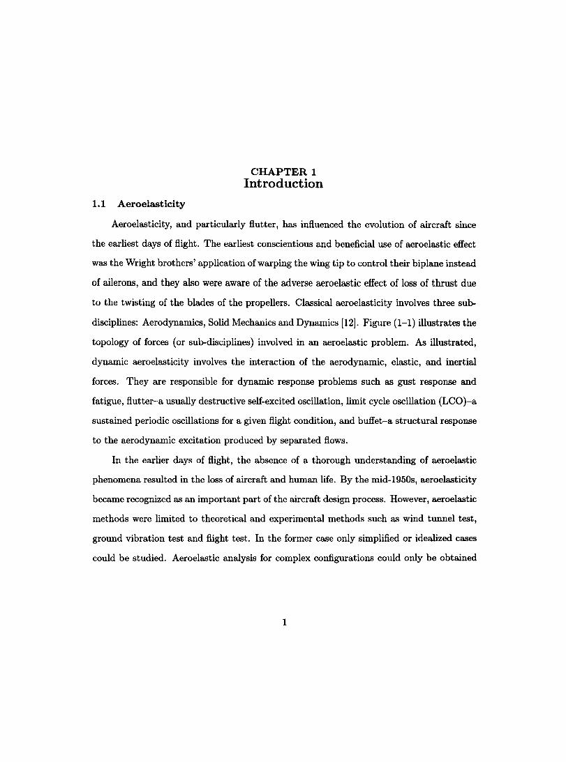
disciplines: Aerodynamics, Solid Mechanics and Dynamics [12]. Figure (1-1) illustrates the

topology of forces (or sub-disciplines) involved in an aeroelastic problem. As illustrated,

dynamic aeroelasticity involves the interaction of the aerodynamic, elastic, and inertial

forces. They are responsible for dynamic response problems such as gust response and

fatigue, fiutter-a usually destructive self-excited oscillation, limit cycle oscillation (LCO)-a

sustained periodic oscillations for a given fiight condition, and buffet-a structural response

to the aerodynamic excitation produced by separated fiows.

In the earlier days of fiight, the absence of a thorough understanding of aeroelastic

phenomena resulted in the loss of aircraft and human life. By the mid-1950s, aeroelasticity

became recognized as an important part of the aircraft design process. However, aeroelastic

methods were limited to theoretical and experimental methods such as wind tunnel test,

ground vibration test and fiight test. In the former case only simplified or idealized cases

could be studied. Aeroelastic analysis for complex configurations could only be obtained

1

StaticAeroelasticity

A: Aerodynamic Forces (Aerodynamics) E: Elastie Forces (Solid Mechanics) 1 : Inertial Forces (Dynamics)

Figure 1-1: Topology of Forces in Aeroelasticity Problem

through experimental methods, however, the large expense and long periods of preparation

limited its use to a handful of flight conditions.

Fortunately, the advent of the digital-computer and the recent increase of comput­

ing power at low price brought considerable changes to the field of aeroelasticity. On the

one side, computational structural dynamics (CSD) using finite element (FE) method has

proved to be computationally efficient to solve aerospace structural problems [24]. On the

other side, computational fluid dynamics (CFD) has emerged as a practical technology to

numerically solve alllevel of fluid equations from the simple potential equation to the com­

plex Navier-Stokes equation [20]. By coupling CFD and CSD methods, larger aeroelastic

systems with more degrees of freedom can be analyzed [31]. Based on these achievements

(not only including ab ove mentioned success), Computational Aeroelasticity (CAE), which

refers to the coupling of high fidelity CFD methods to structural dynamics (SD) tools to

perform aeroelastic analysis, entered into the design phase of aircraft.

2

Generally, there are three approaches to couple CFD and CSD tools: full coupling,

tight coupling and loose coupling. In the full coupling approach, the governing equations

are reformulated to combine both the fluid and structural equations into a single set of

equations [5]. The CFD and CSD equations can then be solved and integrated in time si­

multaneously, allowing a zero time lag between the structural modelloads and aerodynamic

forces. The coupling between fiuid and structure naturally occurs as the result of shar­

ing the degrees of freedom at the fluid-structure interface. However, since the structural

system is physically much stiffer than the fluid system, the numerical matrices associated

with structural equation are orders of magnitude stiffer than those associated with the

fluid solver. Therefore, it is numerically inefficient or even impossible to solve the entire

system using a single numerical scheme. Methods have been developed for the fully cou­

pIed methods, but they are restricted to two dimensional and small-scale three dimensional

problems.

In a tight coupling approach, fluid and structural equations are solved separately and

loads and displacements between the CFD and CSD codes are exchanged at every time step.

Although the actual structural model loads lag the aerodynamic loads by one time step,

if the time step used is small, no significant lag is introduced to the fluid solver, and the

accuracy and stability of both the fluid and structural equations are ensured. At the end of

each time step, the structural dynamic solver predicts a new structural configuration which

is used to determine a new surface mesh for the CFD grid. On the other hand, the new

load distribution obtained from the CFD solver is transfered to the structural mesh. This

can be called a CSD/CFD cycle. Before continuing to the next time step, the cycle repeats

until a converged solution within a specified tolerance is obtained. The tight coupllng

approach could either be implemented as an integrated or modular type. In the case of an

integrated tight coupling method, either the CFD or CSD source code should be altered to

3

include the coupling scheme. The codes are then compiled together and each have access

to the physical memory of the other. A modular tight coupling approach consists of three

separate modules: CFD, CSD and Fluid-Structure Interaction (FSI), allowing a variety of

combinat ion of CFD/CSD codes. In an aircraft design phase, a modular tight coupling

approach will allow the engineer to increase the fidelity of either the CFD or CSD without

altering the coupling approach. At the initial stages of the design phase, the CFD module

can be represented by the solution to the potential equations and the CSD module can be

represented by simple beam theory. As the design progresses, the flow field cau be solved

instead by the Euler equations or ultimately the Navier-Stokes equations and the structure

can be represented by a full Finite Element model.

In the loose coupling approach, the CFD and CSD equations are solved alternatively

with occasional interactions only. Here, CFD analysis are updated by structural deflection

only after several flow field time steps [41]. Unfortunately, this coupling approach is sus­

ceptible to convergence issues due to the inability to capture feedback effects between the

aerodynamic pressure and the structural deflection.

In the aeroelasticity analysis, the simulation of transonic flow is significantly more

complicated than that of either the subsonic or supersonic flight regime due to the nonlin­

earity introduced by the presence of shock waves. When a wing is immersed in transonic

flow, shock waves can form or disappear as the wing undergoes unsteady structural deflec­

tions. Regions of separated flow may appear or disappear as the shock wave strengthens

or weakens. These nonlinear characteristics could lead to flutter, limit cycle oscillations

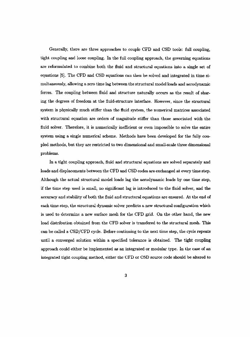
(LCO), buzz of control surface or other nonlinear phenomena. Figure (1-2) shows the flut­

ter boundary of a two dimensional sweptback wing section model in transonic flow, which

is extensively used in many CAE simulation cases. In the transonic speed range, with the

increase of Mach number, the flutter boundary dips and then rises again. Therefore, to

4

2.5r--....,......----.---.---....,......----.---.---....,......-~

2

:> 1.5

j

Il •

0.5 ................ . .la. .la.

..................•

o~-~-~--~-~-~--~-~-~ ~ M ~ V ~ M ~ M ~

Mach Number

Figure 1-2: Transonic Dip of Two-dimensional Sweptback Wing Model

dearly understand the mechanism of Transonic-dip and to accurately predict the fiight

envelope are two of the primary focus of aeroelastic analysis. In this research, the flutter

phenomena in transonic regime for a airfoil and that in subsonic regime for a wing are

studied in the time domain.

1.2 Literature Review

1.2.1 Previous CFD/CSD work

In the early days of flutter analysis, the flutter boundary in transonic regime was

extrapolated from the flutter analysis results in both the subsonic and supersonic regimes.

Later, Isogai [28,29] predicted the flutter boundary using the traditional frequency-domain

technique, where the aerodynamic forces were obtained with the double-Iattice method

(DLM) which is based on linear aerodynamic theory, and the transonic small disturbance

(TSD) method which can capture the nonlinear characteristic of transonic flow. These

methods often over-predicted the Butter boundary, especially in the transonic speed range.

5

Thus a new model that includes the important nonlinear aerodynamic effects such as a

shock wave need to be developed.

Bennett et al. [7] developed the Computational Aeroelasticity Program-Transonic

Small Perturbation (CAP-TSD) method to perform transonic aeroelastic analysis by cou­

pling the transonic small disturbance potential flow equation with the natural vibrational

mode-based structural equations. The TSD potential equation was solved with a modified

AF algorithm [4] using the finite-difference method. The structural equation of motion

were solved on a sheared Cartesian grid where the lifting surface were modeled as a thin

plate. This kind of approach simplified grid generation and no deforming mesh algorithm

was required as the surface velo city boundary condition was applied at the mean plane.

Despite of its high efficiency in computation, this technology might fail in the presence of

a strong shock due to the inability for the potential equations to compute the entropy and

vorticity [20].

To overcome this problem, Batina et al. [4] solved the flow field using the Euler equa­

tions on an unstructured grid. The aeroelastic solution was obtained by tightly coupling the

mode-shape-based structural equations with the Euler equations. The CSD code was inte­

grated into the CFD code, CFL3D. In this method, the Euler equations were solved using

the three-dimensional upwind-type solution algorithm, which permits very large time steps.

The structural system of equations were used to obtain the generalized coordinates at the

CFD grid nodesj and the resulting aeroelastic displacement at any time can be described

as a linear combination of a finite set of modes weighted with the generalized coordinates

under the linearity assumption of modal analysis (mode superposition method) [10]. How­

ever, the increasing use of composite materials for aeroelastic tailoring and the nonlinear

nature of transonic flows make this linearization assumption less attractive. Conversely,

when using the finite element equation, there is no harmonie motion assumption, and the

6

stress acting on the surface of the structure can be obtained directly, resulting in a more

reliable computation, however, the CPU time and storage increases.

Guruswamy et al. [20, 21J developed a procedure (ENSAERO, version 1.0) to solve

simultaneously the Euler flow equations and modal structural equations of motion for

computing the aeroelastic response of a wing. The flow field equations were solved using

a Beam-Warming central-difference scheme on a C-H grid. The aeroelastic equation of

motion was solved by a numerical integration technique based on the linear-acceleration

method [25]. The total displacements of the wing were obtained by superposing the dis­

placements from each mode. Schuster et al. [38J coupled a 3-D flow solver with a linear

structure model to study the aeroelastic analysis of a flight aircraft (ENS3DAE version

1.0). Thin layer approximation of the full 3-D compressible RANS equations were used.

The Beam-Warming implicit scheme was implemented for time integration, and the set

of the discrete flow field equations were solved on a multi-block curvilinear grid. A mesh

deformation algorithm that uses an algebraic shearing technique was used to account for

the grid movement. The structure was modeled with linear generalized mode shapes.

Liu et al. [34J presented an integrated CFD and CSD method for simulation and

prediction of flutter based on an unsteady, parallel, multi-block, multi-grid finite volume

algorithm solving Euler IN avier-Stokes equations. The solution of the flow field was tightly

coupled in time with the solution of the structural modal dynamic equations extracted

from finite element analysis. A dual-time step algorithm was employed to compute the

flow field at each time step. A moving mesh method based on transfinite interpolation

(TF1) [16J and spring analogy was integrated into the code.

Other similar works [6, 30, 22, 21, 14J have also approached the problem of aeroe­

lasticity by using tightly coupled high fidelity CFD and CSD methods. Often these tight

7

coupling approaches, were implemented in an integrated fashion, not allowing a wide vari­

et y of CFD and CSD codes to be used. To allow for greater flexibility, a modular coupling

approach can be used. Generally, the modules include the flow solver module, structural

solver module and Fluid-Structure Interface (FSI) module, which control the communi­

cation between the flow and structural solver modules. For instance, MDICE [39] allows

different flow solvers such as CFD-FASTRAN (CFD Research Corporation) and WIND

(Boeing), and structural solvers such as FEMSTRESS (CFD Research Corporation) and

NASTRAN to be used to perform aeroelastic analysis.

1.2.2 Mesh Deforming Aigorithm

In each CFDjCSD cycle, the interior fluid grid points must be computed based on

the deformation on the surface, which are based on the solution to the structural equation

of motion. A variety of mesh deforming algorithms have been carefully designed. The

simplest and most robust method is to globally re-mesh the interior nodes based on the

surface nodes [17], however, this pro cess is computationally costly.

The most common methods perturb the interior nodes of the existing grid. A proven

technique for perturbing structured single block grids is the algebraic shearing process [45].

In this method, grid points along a grid line that connect the body surface to the far-field,

are shifted along the same grid line. The surface displacement is gradually decayed to zero

at the far-field, and rotational movement can be added to maintain orthogonality at the

surface. This scheme is easy to implement, but, large displacements can have an adverse

effect on grid quality.

The spring analogy scheme, initially developed by Batina [4], is usually applied to grid

perturbation on unstructured triangular or tetrahedral grids. Here, the mesh is modeled

as a network of springs, and the edges of each computational cell represents a linear spring

whose stiffness is inversely proportional to a specified power of the edge length. Robinson et

8

al. [37] extended this scheme to structured grids where diagonallinear springs were added

along the surface of the celi in order to control celi shearing and to prevent the collapse of a

cell. Similarly, the stiffness of the diagonal springs are inversely proportional to the length

of the diagonal raised to a power. Farhat et al. [18] proposed a modified spring analogy

by adding additional nonlinear torsion spring to avoid the negative celi volume problem

associated with the linear spring network. However, spring analogy methods require con­

siderable computer resource in terms of memory and CPU time and have wider use on

unstructured meshes where structured 3D interpolation methods are not as applicable.

'fransfinite Interpolation (TF1) is another widely-used efficient technique for generat­

ing structured computational grids [15]. Here, the coordinates of points at the vertexes and

edges (and in three dimensions, from the block faces) are interpolated to locate grid points

in the interior of the integration domain. TF1 combines the speed and efficiency of an alge­

braic method with the ability to handle fully 3D perturbation. Wong et al. [50] combined

the TF1 and spring analogy to re-mesh adaptively in each grid block. An arc-Iength-based

transfinite interpolation is used to move the grids within each block. A spring network

approach is then applied to determine the motion of the corner points of the blocks and a

smoothing operator is introduced to maintain the grid smoothness and grid angles.

Another class of method for re-meshing is by solving a partial differential equation.

Holmes et al. [27] move the grid points in the interior of the flow domain by solving the

Laplace equation V'2u = 0 for each of the three components of the displacement with the

Dirichlet boundary condition imposed on aIl boundaries. This method can maintain grid

point concentration for small displacements, but for large displacements, it can lead to

mesh degeneracies near sallent corners of the geometry. Mittal et al. [35] proposed that

within a smali region around the body, elements move rigidly with the body. However, this

9

Transferto FEMGrid

F1uidlStructure Interface

Move Transferto u Grid CFDGrid

Figure 1-3: Modular Coupling Aeroelastic Analysis

proved to be applicable only to simple rotations and translations. A new two-zone grid­

moving approach with enhanced robustness was presented by Lepage et al. [33]. Here, the

displacements of interior grid points in both zones were smoothed by solving the Laplace

equation with Neumann boundary conditions ~ = 0 on the external boundary of the inner

zone. The mesh deformation procedure employed in this work will use a two-zone method.

1.2.3 Fluid-Structure Interface Model

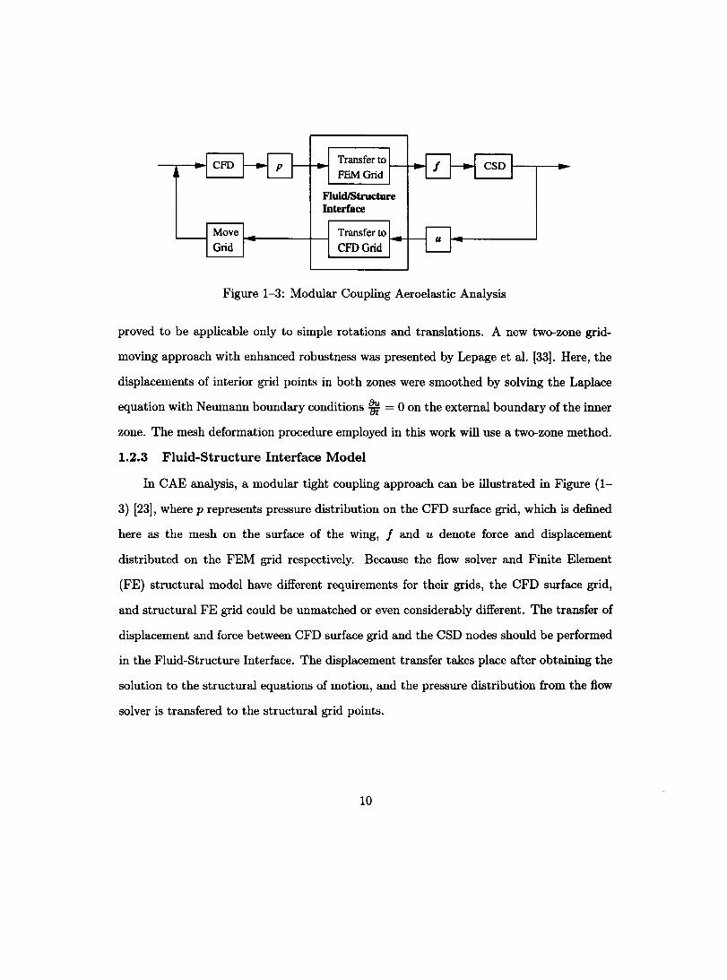
In CAE analysis, a modular tight coupling approach can be illustrated in Figure (1-

3) [23], where p represents pressure distribution on the CFD surface grid, which is defined

here as the mesh on the surface of the wing, f and u denote force and displacement

distributed on the FEM grid respectively. Because the flow solver and Finite Element

(FE) structural model have different requirements for their grids, the CFD surface grid,

and structural FE grid could be unmatched or even considerably different. The transfer of

displacement and force between CFD surface grid and the CSD nodes should be performed

in the Fluid-Structure Interface. The displacement transfer takes place after obtaining the

solution to the structural equations of motion, and the pressure distribution from the flow

solver is transfered to the structural grid points.

10

Numerous CFDjCSD interpolation algorithms have been developed in the CFD com­

munity. Among them, the method of Infinite-plate splines (IPS) [26], which is used exten­

sively in programs such as ASTRO, MSCjNASTRAN [43,42], is based on a superposition

of the solutions for the partial difIerential equation of equilibrium for an infinite plate.

Using the solution of the IPS, a set of concentrated loads are calculated that gives rise to

the required deflection. These concentrated forces are substituted back into the solution to

provide a smooth surface passing through the data. The deflection of the CFD grid points

can be easily calculated from the deflection of the structural grid points. However, this

method does not conserve the work done by the aerodynamic forces and requires fine grids

from both the fluid and structural system to provide accurate results [23].

Guruswamy et al. [24] presented a virtual surface (VS) method based on the mapping

matrix developed by Appa [2]. Here, a virtual surface was introduced between the fluid

surface grid and the FE mesh for the wing. Both the displacement of surface grid points

and structural FE nodes can be expressed as the product of a mapping matrix and the

global displacement vector. By forcing the deforming VS to pass through the given data

points of the deformed structure, the relationship between the displacement of aerodynamic

surface grid points and structural grid points can be built with a derived mapping matrix

[TjT. From the principles of virtual work, the nodal force vector of aerodynamic grid

points can be mapped onto the structural grid points with the matrix [T]. This approach

not only accommodates changes in fluid and structural models easily, but also conserves

the work done by the aerodynamics when obtaining the global force vector. However, the

requirement of intermediate modeling between fluid and structural models may lead to

more complicated coding and more expensive computations.

Tzong et al. [48] developed a node-to-element approach. Here, the FE grids are gen­

erated using an iso-parametric element, and surface grid nodes are projected directly onto

11

the adjacent elements of the FE model. Then the relationship between the displacement

of surface grid nodes and the displacement of the projected point on the FE element can

be written in a matrix format Ua = [F]us , where Ua contains three translational displace­

ment components of the surface grid point, Us consists of three translational and three

rotational displacement components of the finite element, and [Pl is the mapping matrix

which depends on the location of the surface grid point, the location of the projected finite

element and the offset distance from the surface grid point to the element surface. Using

the inverse matrix of [F] the force calculated from the flow solver can be proportionately

distributed to the structural nodes, and the work done by the aerodynamic force is consis­

tently transfered to the FE model. Brown [8] developed a similar scheme, and combined

them with the lumped method for wing-box structure to interface data between fluids and

structure. Chen et al. [9] proposed an alternative approach based on a boundary element

concept and applied it to a blended wing body configuration.

1.3 Thesis Objective

The research conducted in this thesis concentrated on two main objectives:

1. Coupling typical wing section model and flow solver to find the flutter boundary in

transonic regime with transient response method.

2. Developing a new fluid-structure interface algorithm.

3. Using the above interface algorithm in computational aeroelastic analysis to find a

flutter point of a real wing in subsonic flow.

The equations of motion of a typical section model is solved with the ,B-Newmark

scheme, the Euler equations of fluid flow around the model is solved with the flow solver-FENSAP,

and the virtual surface method is used to transfer load and displacement between fluid sur-

face grid and the FE nodes. This framework is applied to the NACA64010 airfoil to

12

calculate the fiutter points of a sweptback wing section at different transonic Mach num­

bers.

Using the new fiuid-structure interface algorithm, the fiow solver-FENSAP is coupled

with the structural solver-N ASTRAN to predict the subsonic flutter point of the AGARD

wing 445.6 at a Mach number of 0.499.

The results in both test cases are compared with previous numerical and experimental

results.

13

CHAPTER 2 Governing Equations

Aeroelastic analysis constitutes two main components: unsteady aerodynamics and

structural analysis. First, the goveming equations of unsteady aerodynamic flow based on

conservation laws are presented in the Eulerian reference frame. Second, the structural

equations of models are formulated in a Lagrangian reference system.

2.1 Governing Equations of Flow

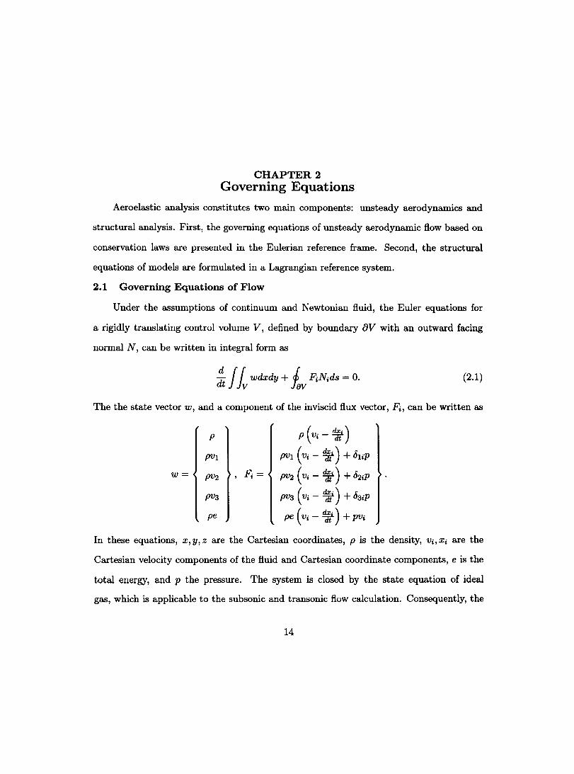
Under the assumptions of continuum and Newtonian fluid, the Euler equations for

a rigidly translating control volume V, defined by boundary av with an outward facing

normal N, can be written in integral form as

(2.1)

The the state vector w, and a component of the inviscid flux vector, Fi, can be written as

p P (Vi - ~) pv! pv! (Vi - ~ ) + 8liP

w= PV2 ' Fi = PV2 (Vi - ~ ) + 82ip

PV3 PV3 (Vi - ~ ) + 83ip

pe pe ( Vi - ~ ) + PVi

In these equations, x, y, z are the Cartesian coordinates, p is the density, Vi, Xi are the

Cartesian velocity components of the fluid and Cartesian coordinate components, e is the

total energy, and P the pressure. The system is closed by the state equation of ideal

gas, which is applicable to the subsonic and transonic flow calculation. Consequently, the

14

"

Figure 2-1: Two-DOF Wing Section Model Geometry and Parameters

pressure, p, can be expressed as

(2.2)

where'Y represents the ratio of specific heats. The total enthalpy is also related to the total

energy and pressure by

h = e+~. p

2.2 Governing Equation of Structure

(2.3)

In this section, the structural equations of motion are introduced. Two structural

models are presented: first, a two degree of freedom wing section model; second an isotropie

3D linear structural model.

2.2.1 Typical Wing Section Model

To simulate the movement of wing sections, the wing section is elastically mounted

on the base, and it is permitted to move in pitch about a given elastic axis and plunge

vertically. The elastic axis is defined by a in term of semi-chord length b with the origin

point located at the mid-chord position. If a is positive, it means that the axis is located

downstream of the mid-chord, and negative if the axis lies upstream of the mid-chord.

15

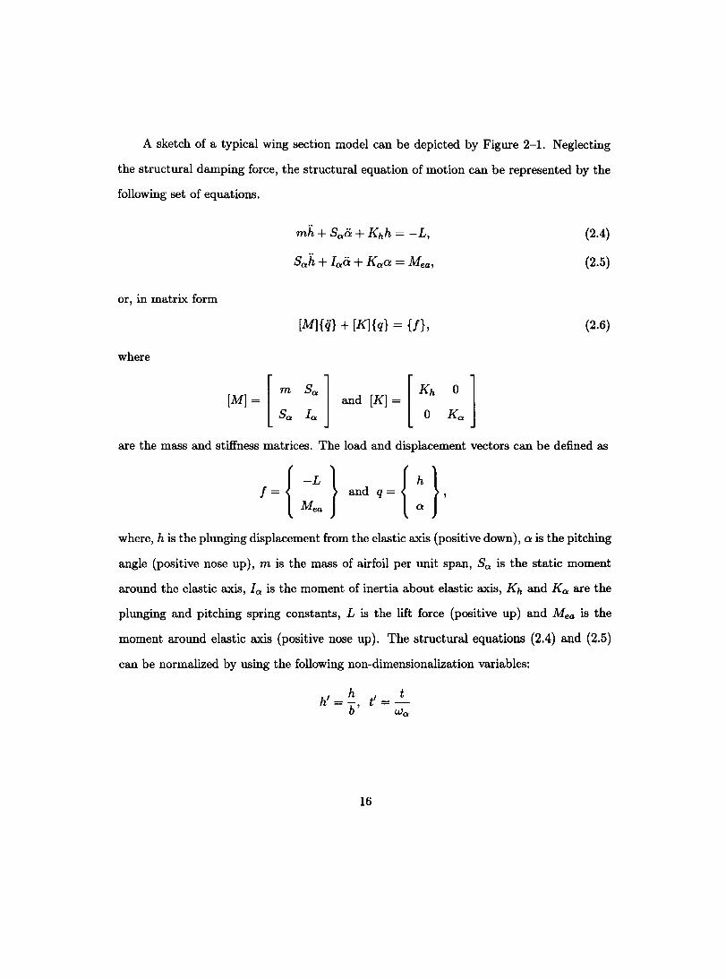
A sketch of a typical wing section model can be depicted by Figure 2-1. Neglecting

the structural damping force, the structural equation of motion can be represented by the

following set of equations.

or, in matrix form

[M]{q} + [K]{q} = {i},

where

and [K] = [Kh 0 1 o Ko;

(2.4)

(2.5)

(2.6)

are the mass and stifIness matrices. The load and displacement vectors can be defined as

where, h is the plunging displacement from the elastic axis (positive down) , a is the pitching

angle (positive nose up), m is the mass of airfoil per unit span, 80; is the static moment

around the elastic axis, Jo; is the moment of inertia about elastic axis, Kh and Ko; are the

plunging and pitching spring constants, L is the lift force (positive up) and Mea is the

moment around elastic axis (positive nose up). The structural equations (2.4) and (2.5)

can be normalized by using the following non-dimensionalization variables:

h'-!!: t'=~ - b' Wo;

16

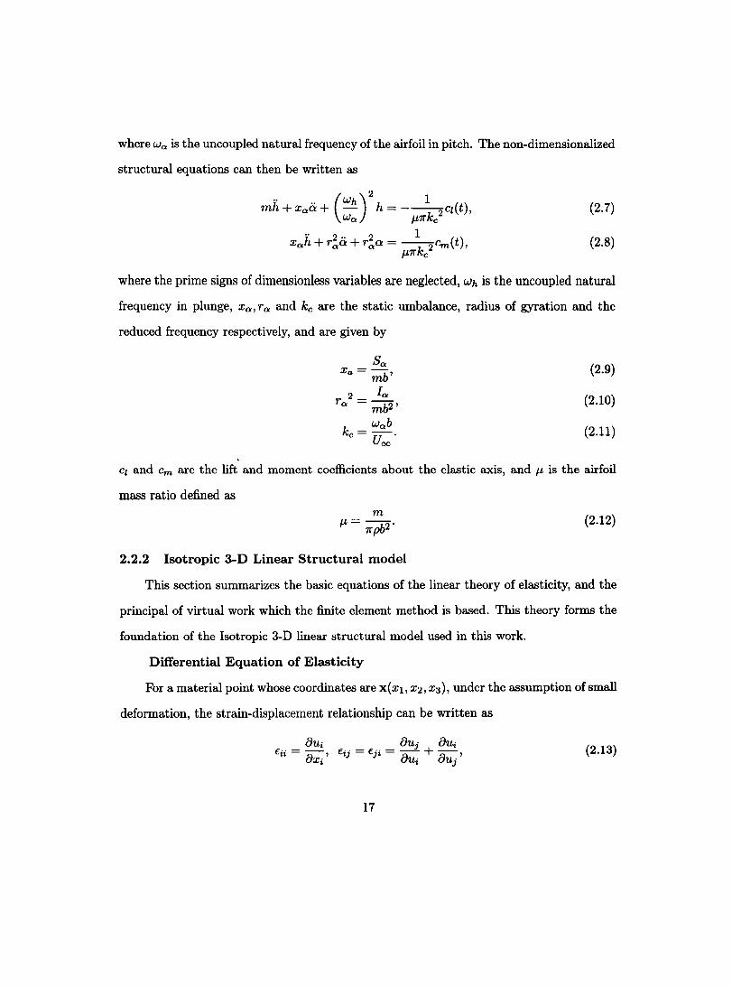
where Wo: is the uncoupled natural frequency of the airfoil in pitch. The non-dimensionalized

structural equations can then be written as

(2.7)

(2.8)

where the prime signs of dimensionless variables are neglected, Wh is the uncoupled natural

frequency in plunge, Xa , ra and kc are the static umbalance, radius of gyration and the

reduced frequency respectively, and are given by

r~2 -~ - mb2'

k _ wab

c - Uoo

'

(2.9)

(2.10)

(2.11)

Cl and Cm are the lift and moment coefficients about the elastic axis, and /-L is the airfoil

mass ratio defined as m

/-L = 1rpb2 ' (2.12)

2.2.2 Isotropie 3-D Linear Structural model

This section summarizes the basic equations of the linear theory of elasticity, and the

principal of virtual work which the finite element method is based. This theory forms the

foundation of the Isotropie 3-D linear structural model used in this work.

Differentiai Equation of Elasticity

For a material point whose coordinates are X(Xl, X2, X3), under the assumption of small

deformation, the strain-displacement relationship can be written as

8Ui 8uj 8Ui €ii = -8 ' €ij = €ji = -8 + -8 '

Xi Ui Uj (2.13)

17

where fii and fij are the three normal strain components and six shear strain components

respectively, Ui is the three components of the displacement vector u of that point.

If the structure is homogeneous and isotropie and the displacement is small, the strain­

stress relationship are given by

(2.14)

where O"ii and O"ij are the three components of normal stresses and six shear stresses re-

spectively, and

À = 1/E (1 + 1/)(1 - 21/)'

E Il- = 2(1 + 1/)'

where E is Young's modules, and 1/ is Poisson's mtio.

For a small moving particle with unit volume, the equation of motion can be derived

from the equilibrium of internaI and external forces applied to it. Under the dynamic

loading condition, the inertial force -pü, should be considered, and the dissipation of

energy during vibration is taken into account by adding a velo city dependent damping force

-~u, where ~ is the coefficient of viscous damping per unit volume. Thus the equation of

motion in the i-direction can be written as

ÔO"ij .. • F -ô + PUi + ~Ui = Bi,

Xj (2.15)

where FBi represents the body force in the i-direction. These three equations should hold at

the x, y, and z directions at every point of the structure. The stresses O"ij vary throughout

the structure, and at its boundary surface they must be in equilibrium with the external

forces acting on the surface.

18

Principle of virtual displacement

The exact solution to equation (2.15) is feasible to sorne special cases, however, for

a general structure, it can be approximately solved by using the energy method. Energy

methods are restricted to small deformations such that the equation that relates strain to

displacement remain linear. The principle of virtual work which is one of the more preferred

energy methods states that a structure under the action of a set of forces is in equilibrium,

if the virtual work is equivalent to the virual strain for any virtual displacement, 8u. In a

fact, the method assumes that while the structure is displaced from u to u + 8u, the forces

acting on the structure remain constant. As a result, for a system described by equation

(2.15), the virtual work done by the stress, inertial, damping and body forces should equal

to zero. This relationship can be derived by integrating the product of Equation (2.15)

and the virtual displacement 8u over the structural system,

r (ÔÔO'ii + piii + KUi) 8udV = r p8udS, lv xi lav

(2.16)

where the the right hand side denotes the work done by the aerodynamic pressure on the

boundary surface of the structure. Introducing the stress vector u and the strain vector E

AU fU

0'22 f22

0'33 f33 u= , E=

0'12 f12

0'23 f23

0'31 f31

equation (2.16) can be cast into

r 8ET udV = r p8udS - r 8u[pü + Kü]dV. lv lav lv

(2.17)

19

2.3 FluidjStructure Interaction

Since the fluid and structure do not mix, there exists an interface such as a 2D man-

ifold in 3D space, in which the fluid and structure interact on each other. Therefore, in

the process of constructing the governing equations for a continuous system in fluid and

structural domains, the displacement and pressure field should remain identical in both

domains. Similarly, for the computation of an aeroelastic system with the discretized for-

mulation, these two identities should be maintained by some mathematical principle. As

examples of such princip les , the conservation of loads and energy in terms of load transfer

from the fluid to the structure, and the geometric conservation law in terms of displacement

transfer from structure to the fluid are introduced in this section.

2.3.1 Conservation of Load and Energy

The surface of the structure can be discretized into a set of finite number of elements.

When the distributed pressure load is applied to a finite element, it must be transformed

into an equivalent set of point forces at the nodes. The transformation must satisfy two

criterias. First the total forces acting on the structure must be equivalent to the totalloads

computed on the fluid grid by integrating pressure over the surface. Thus conservation of

load must be satisfied, which can be represented by

L f(m) = la pdS, m av

(2.18)

where f{m} is the nodal force vector at the node m of the structural system.

Second, the virtual work done by the nodal forces f{m} by perturbing the structural

nodes by a virtual nodal displacement 8q should be equal to that done by the original

20

distributed pressure load p moving through an equivalent virtual displacement 6u, namely,

This is called conservation of energy.

2.3.2 Geometrie Conservation Law

(2.19)

In computational aeroelastic analysis, when the structure experiences a displacement

movement, the wall boundary surface of the flow system should have a consistent displace­

ment. The geometric parameters of the wall boundary surface nodes of the flow mesh must

satisfy the geometric conservation law [47J, which states that the computation of the geo­

metric parameters must be performed such that the resulting numerical scheme preserve

the state of a uniform flow, independent of the mesh motion. Its integral form given by

Farhat et al [18J is cast as

dd r dV(t) = r (b.n)dS(t) t Jv Jav

(2.20)

where n represents the outward unit vector, b denotes the local boundary velocity varying

over the surface S(t) of the control volume.

21

CHAPTER3 Methodology Description

Computational Aeroelastic analysis involves the simultaneous computation of the

structural equations of motion and the fluid equations to estimate the dynamic response of

an elastic structure. An accurate response can only be acquired by a consistent coupling

of the two disciplines. The flow solver provides the pressure distribution over the aircraft

surface, which is conservatively transfered to the structural surface. The solution to the

structural equations of motion provides the displacement at each node at a given time.

Subsequently, the displacement is transfered to the fluid grid, and a new solution to the

fluid equations are acquired based on the new aircraft surface deflections.

This chapter presents the computational methods for the flow solver in section 3.1

and the structural solver in section 3.2 respectively. Section 3.3 depicts the fluid/structure

coupling procedure.

3.1 Flow Solver

In the present study, the flow solver employed is the Finite Element Navier-Stokes

Package (FENSAP), developed by the CFD Laboratory at McGill University. It is ca­

pable of simulating three-dimensional laminar /turbulent, steady /unsteady, compressible

Euler/Navier-Stokes flow for a wide range of industrial applications. Based on a fully im­

plicit finite element formulation with the Arbitrary Lagrangian-Eulerian (ALE) algorithm,

the continuity and momentum conservation equations are solved in a strongly coupled fash­

ion for pressure p and velo city components Ui (i = 1,2,3) by lagging the density p. The

22

temperature T is obtained by solving the equation for conservation of energy. Finally the

density, p, is computed from the equation of state for ideal gas.

3.1.1 Weak-Galerkin Formulation

The weak-Galerkin formulation of Euler equation can be obtained by rewriting the

non-dimensional governing equation (2.1) in differential form, and then integrating it over

the fluid domain with respect to the weighted function W(x). The formulation is then cast

in terms of a first-order derivative, and not the original second-order derivative form. The

transformed integral form of the continuity and momentum equations can be written as,

1 { dp dXi âp } 1 1 - W ---- dV+ W·pv·dV- Wpv·n·dS=O V dt dt ÔXj v,) J S J J ,

(3.1)

_ f w{dPVi _ dXj (pâVi +Vi~)}dV Jv dt dt âXj âXj

+ Iv W,j {pvjVi + 8ijp} dV

-!s W {pvjVi + 8ijp} njdS = 0, (3.2)

where i = 1,2,3. Replacing e with T by using equation (2.3), the integral form of the

energy equation can be written as

-Iv W {pCp [~ + (Vj - d::) T,j - h - I)M! (: + (Vj - d::) p,j) ] } dV = O.

(3.3)

3.1.2 Artificial Viscosity

In order to stabilize the numerical scheme, artificial viscosity is added to the right-hand

side of the equations. The general form of the dissipation terms are

23

RGScont = Iv V' . {ha [(Ei + E~) V'p - E~V'p]} dV,

RGSi - mam = Iv V' . {ha [(EÏ + E2) V'Vi - E2V'Vi]} dV,

RGSenergy = Iv V'. {ha [(Er + En V'T - EfV'r]} dV,

(3.4)

(3.5)

(3.6)

where the coefficients Ei,EÏ,Er,E~,E2,Ef control the fust-and second-order artificial

dissipation added to the continuity, momentum and energy equations respectively, and ha

denotes a locallength scale h of the element, raised to the power a (a = 0 or 1). This

formulation allows for the variation of the magnitude of the artificial viscosity term based

on the local element size. A shock detector based on the pressure gradient turns off the

second-order term in the vicinity of shock waves to produce a pure upwind scheme [3].

3.1.3 Spatial Discretization

In the finite element method, the flow domain of interest is discretized into a collection

of small elements enclosed by the boundary surface (including real and virtual boundaries).

These finite elements are connected by nodes shared by surrounding elements. Then the

coordinate components ~i (i = 1,2,3) of any material point x in the local coordinate system,

at an element level, can be written as a function of its global coordinate components Xi

(i = 1,2,3) of the nodes of that element.

n.

~i = L XiNj(X), j=l

(3.7)

where ne is the number of nodes of the element, the interpolation function Nj(x) is the

shape function of the element expressed in local coordinates. This shape function depends

on the element geometry, number of nodes, and is also used to express the property pa-

rameters </>(x) of the same point in terms of the property parameters of the nodes of the

24

element, ne

4J(X) = L 4Jj Nj (x). (3.8) j=l

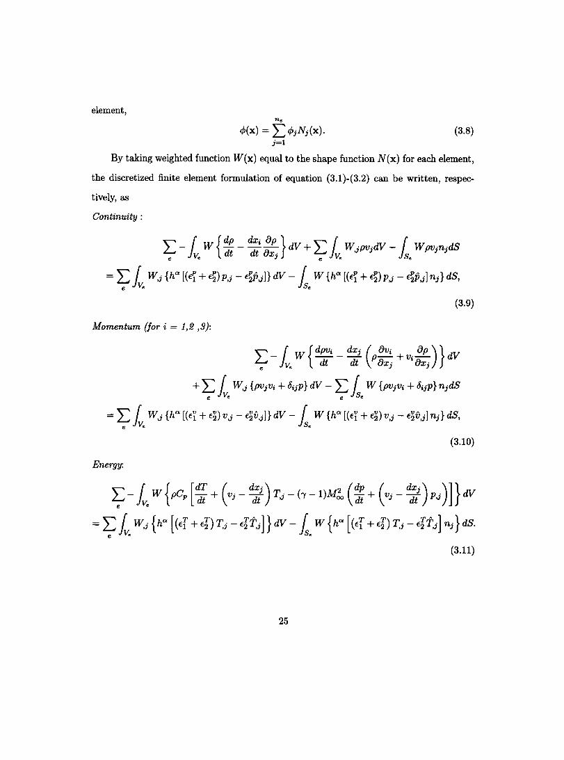
By taking weighted function W(x) equal to the shape function N(x) for each element,

the discretized finite element formulation of equation (3.1)-(3.2) can be written, respec­

tively, as

Continuity :

Momentum (for i = 1,2 ,3):

= L [ W,j {ha [(il + €2) V,j - €2V,j]} dV - [ W {ha [(il + €2) V,j - €2V,j] nj} dS, e JVe JSe

(3.10)

Eneryy:

~ -le W {pep [~~ + (Vj - d;:) T:j - h - 1)M! (dt + (Vj - d::) P,j)]} dV

=L [W,j{ha[(€f+€nT,j-€It:j]}dV- [W{ha[(€f+€nT,j-€ITJ]nj}dS. e JVe JSe

(3.11)

25

3.1.4 Time Discretization

A backward difference formula, based on Gear's method, is employed to discretize the

time derivative terms in the time-accurate formulation. Take the ALE time derivative i of a dependent variable f for example, i at time level t can be written as

(:)' = ~t ( ao/I + ~ a;/(I-.8t») , (3.12)

where m is the order of accuracy in time, depending on the number of time levels used.

The second-order formulation is generally used due to the over-diffusion of the first-order

formulation and the highly dispersive third-order formulation.

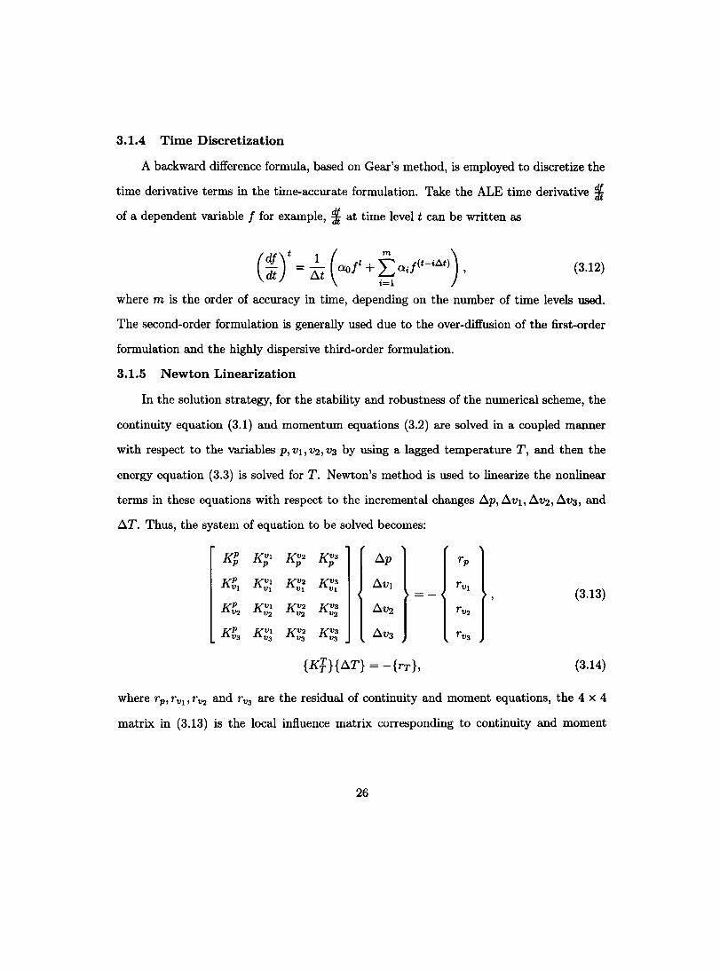
3.1.5 Newton Linearization

In the solution strategy, for the stability and robustness of the numerical scheme, the

continuity equation (3.1) and momentum equations (3.2) are solved in a coupled manner

with respect to the variables p, vI, V2, V3 by using a lagged temperature T, and then the

energy equation (3.3) is solved for T. Newton's method is used to linearize the nonlinear

terms in these equations with respect to the incremental changes ~p, ~VI, ~V2, ~V3, and

~T. Thus, the system of equation to be solved becomes:

KP P

KVi P

K V2 P

K V3 P ~p Tp

K~i KVi K V2 K V3 ~VI TVi Vi Vi Vi (3.13) K~2 KVi

V2 K V2

V2 K V3

V2 ~V2 TV2

K~3 KVi V3

K V2 V3

K V3 V3 ~V3 TV3

{KF}{~T} = -{TT}, (3.14)

where Tp , Tvl' TV2 and TV3 are the residual of continuity and moment equations, the 4 x 4

matrix in (3.13) is the local influence matrix corresponding to continuity and moment

26

equations, TT is the residual of energy equation, and {Kt} is the local influence matrix

corresponding to the energy equation.

At each Newton iteration, the element influence matrices are assembled into two global

matrices. By solving in turn, these two matrices use a preconditioned Generalized Minimal

Residual (GMRES) iterative solver, with the choice of preconditioner depending on the

problem of interest, the incremental changes of p, Vi and T can be obtained.

3.1.6 Time-Marching approach

In the unsteady calculation, to obtain the solution at time level (n + 1) based on the

solution at time level n, the linearized equations are solved with Newton's method. After a

certain number of Newton iterations, if the residuals reach a convergence criteria, then the

solution can advance to the next time step. Due to the reason mentioned in section (3.2.1),

the steady state solution can be obtained with a time-marching approach. The solution

advances in time until the time derivative term becomes zero. Herein, only a single Newton

iteration is performed per time step.

The convergence rate of the Newton iteration can be improved by choosing a local

time step 6.t determined by the CF L number and the value ~t8tab, which varies according

to the size of the element.

~t = CFL· ~t8tab. (3.15)

3.1.7 Boundary Conditions

For inviscid flow, the slip condition is imposed on the wall. For unsteady computations,

the velocity of the surface nodes are computed with the backward difference formula (3.12)

with m set to 1. For the inlet boundary condition, the velocity v and temperature T are

specified as the free-stream velocity and temperature respectively. As for the exit boundary

condition, for a subsonic outflow, the pressure is specified along the entire surface and if

27

supersonic, no back pressure is specified. Lastly, at the symmetric plane, the velocity

component normal to the plane of symmetry is set to zero.

3.1.8 Mesh Deforming Algorithm

For an aeroelastic analysis, the computational fluid dynamic mesh must be deformed

at each time step such that the surface mesh matches the instantaneous shape of the

structural mesh. When the surface nodes of the fluid mesh move at the speed ~, the

nodes between the wall and far-field should be deformed appropriately, to ensure a high

quality mesh at each time step. Mesh distortions or inverted elements can severely affect

the convergence of the flow solver.

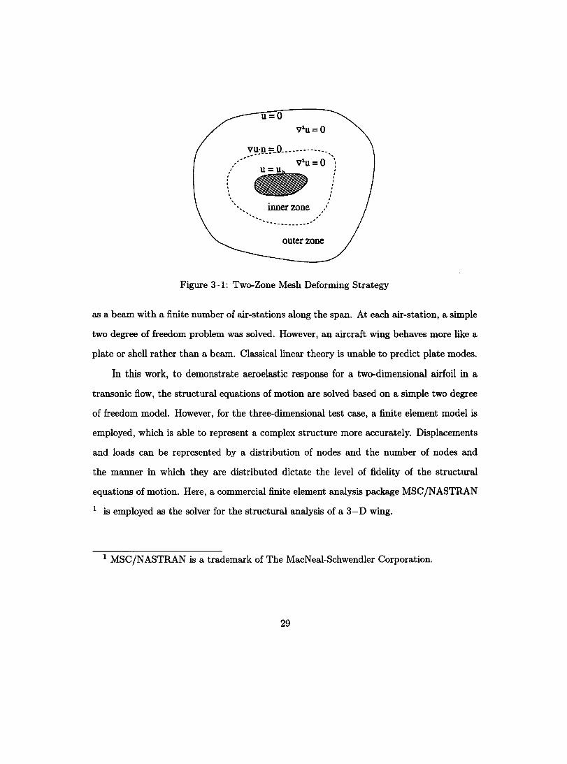
In this work, a two-zone grid-deforming approach with enhanced robustness is used in

the flow solver as illustrated in figure (3-1). In both zones, the displacement is smoothed

by solving the Laplace equation,

(3.16)

In the inner zone, a Dirichet boundary condition is imposed based on the surface grid dis­

placement provided by the structural solver, and a Newman boundary condition Vu· n = 0

is enforced on the external surface of the inner zone. In the outer zone, a Dirichet boundary

condition is imposed on aH boundaries, with the value calculated from the displacement of

the inner zone and u = 0 is set at the far-field boundary.

3.2 Structural Mechanics

Aeroelastic analysis based on classical linear theory, can be obtained by solving a

simple eigenvalue problem using a limited number of degrees of freedom. The displacements

for each degree of freedom can be solved separately and by the method of superposition, the

overall deflections can be computed. Two degrees of freedom problems, one for the plunging

motion and the other for pitching, provide the basis for the majority of early aeroelastic

analysis. These methods were utilized for three-dimensional problems, by treating the wing

28

, , , , , 1 1 1 1 1 ,

, ,

u=o

vu·n = 0 ____________ _ ....... ----- "',

- V2U = 0 :

--- innerzone ---'. -------_.-

outer zone

1 1 1 1 1 1 . , , , ,

Figure 3-1: Two-Zone Mesh Deforming Strategy

as a beam with a finite number of air-stations along the span. At each air-station, a simple

two degree of freedom problem was solved. However, an aircraft wing behaves more like a

plate or shell rather than a beam. Classicallinear theory is unable to predict plate modes.

In this work, to demonstrate aeroelastic response for a two-dimensional airfoil in a

transonic flow, the structural equations of motion are solved based on a simple two degree

of freedom model. However, for the three-dimensional test case, a finite element model is

employed, which is able to represent a complex structure more accurately. Displacements

and loads can be represented by a distribution of nodes and the number of nodes and

the manner in which they are distributed dictate the level of fidelity of the structural

equations of motion. Here, a commercial finite element analysis package MSCjNASTRAN

1 is employed as the sol ver for the structural analysis of a 3-D wing.

1 MSCjNASTRAN is a trademark of The MacNeal-Schwendler Corporation.

29

3.2.1 Finite Element Analysis of Structure

In the finite element method, the structure is discretized into an assembly of finite

structural components (or elements) interconnected at the nodes on the element bound­

aries. Vnder the assumption of small displacements the displacement vector u of any point

x can be written as

(3.17)

where 'I1(m) is the finite-element shape function representing the displacement interpola­

tion matrix, the superscript m denotes the element number m. q(m) is the vector of

nodal displacements for that element, including the three translational components along

the Cartesian coordinate axis and the three rotational components around the same axis.

'I1(m)(x) depends on the element geometry, number of nodes and the degree-of-freedom of

these nodes.

Vnder the same assumption as that in equation (3.17), the corresponding strains at

the element level is written in matrix form using the strain-displacement relationship of

equation (2.13).

(3.18)

where strain-displacement matrix s(m) is obtained by differentiating 'I1(m). Furthermore,

the stresses in each element are related to the strain by the following matrix equation

(3.19)

where E(m) is the elasticity matrix of the element m and its components are given in

equation (2.14). Based on equations (3.17"'3.17), the equation (2.17) for the isotropie

30

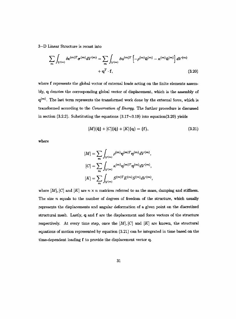
3-D Linear Structure is recast into

(3.20)

where f represents the global vector of external loads acting on the finite elements assem­

bly, q denotes the corresponding global vector of displacement, which is the assembly of

q(m). The last term represents the transformed work done by the external force, which is

transformed according to the Conservation of Eneryy. The further procedure is discussed

in section (3.2.2). Substituting the equations (3.17"-'3.19) into equation(3.20) yields

where

[M]{ij} + [C]{q} + [K]{q} = {f},

[M] = L f pCm)rJ(m)T rJ(m)dv(m) , m }v(m)

[Cl = L f ~(m)rJ(m)T rJ(m)dv(m) , m }v(m)

[K] = L f s(m)TE(m)s(m)dv(m), m }V(nl)

(3.21)

where [M], [Cl and [K] are n x n matrices referred to as the mass, damping and stiffness.

The size n equals to the number of degrees of freedom of the structure, which usually

represents the displacements and angular deformation of a given point on the discretized

structural mesh. Lastly, q and f are the displacement and force vectors of the structure

respectively. At every time step, once the [M], [Cl and [K] are known, the structural

equations of motion represented by equation (3.21) can be integrated in time based on the

time-dependent loading f to provide the displacement vector q.

31

MSC/NASTRAN ofIers two approaches to analyze transient dynamic responses: Modal

or Direct. The former uses a limited number of mode shapes to formulate the equation

in terms of the generalized mass and stifIness matrices that are diagonal matrices, and

recovers the physical response by superimposing the individual modal responses. The later

approach marches the equations forward in time to provide the physical response.

MSC IN ASTRAN, also, provides two types of solution sequences for transient response

analysis with time-dependent loads: the direct linear transient solution sequence (SOL109)

and nonlinear/linear transient solution sequence (SOL129). Although both of them can

perform transient response analysis for linear-element structures, SOL129 is used in the

present study due to the fact that SOL109 does not allow the specification of both initial

displacements and velocities.

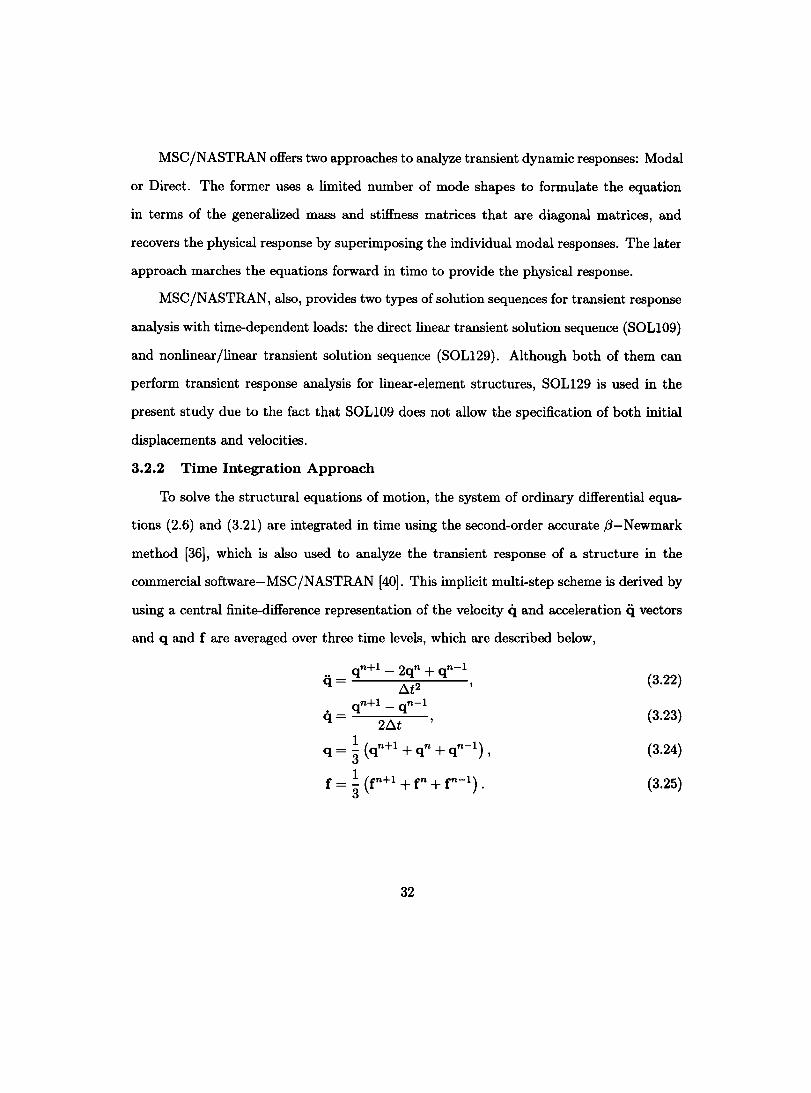
3.2.2 Time Integration Approach

To solve the structural equations of motion, the system of ordinary difIerential equa­

tions (2.6) and (3.21) are integrated in time using the second-order accurate f3-Newmark

method [361, which is also used to analyze the transient response of a structure in the

commercial software-MSC/NASTRAN [401. This implicit multi-step scheme is derived by

using a central finite-difIerence representation of the velocity Ct and acceleration q vectors

and q and f are averaged over three time levels, which are described below,

32

(3.22)

(3.23)

(3.24)

(3.25)

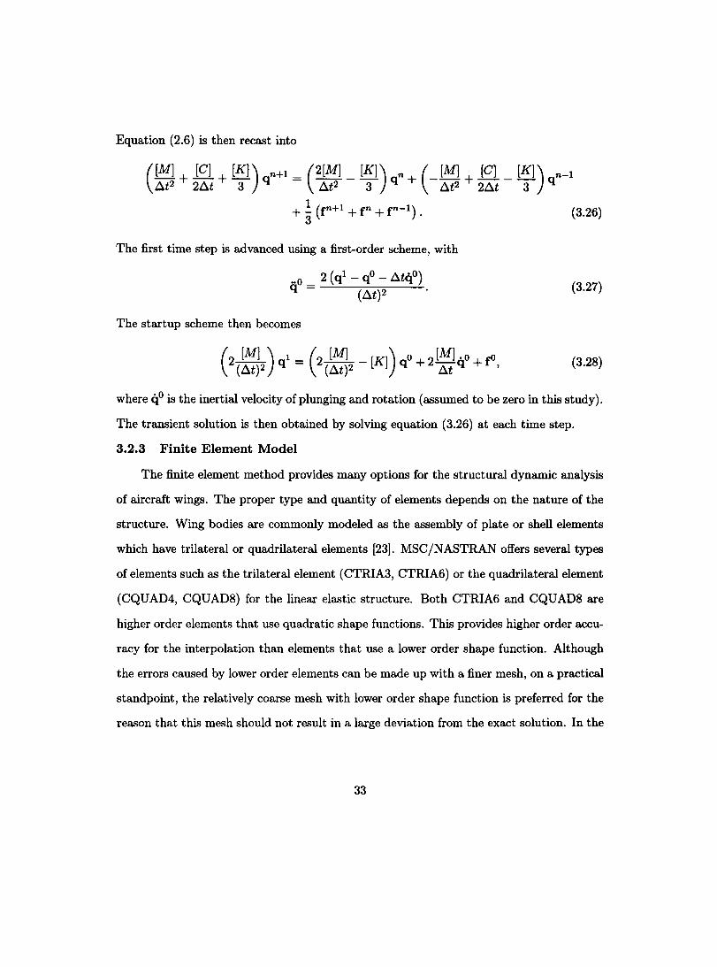
Equation (2.6) is then recast into

([M] + B + [K]) qn+l = (2[M] _ [K]) qn + (_ [M] + B _ [K]) n-l Ât2 2Ât 3 Ât2 3 Ât2 2Ât 3 q

+ ~ (rn+! + rn + rn-l) . (3.26)

The first time step is advanced using a first-order scheme, with

(3.27)

The startup scheme then becomes

( [M]) 1 ([M] ) 0 [M] ·0 CO

2 (Ât)2 q = 2 (Ât)2 - [K] q + 2 Ât q + , (3.28)

where 4° is the inertial velocity ofplunging and rotation (assumed to be zero in this study).

The transient solution is then obtained by solving equation (3.26) at each time step.

3.2.3 Finite Element Model

The finite element method provides many options for the structural dynamic analysis

of aircraft wings. The proper type and quantity of elements depends on the nature of the

structure. Wing bodies are commonly modeled as the assembly of plate or shell elements

which have trilateral or quadrilateral elements [23]. MSC IN ASTRAN offers several types

of elements such as the trilateral element (CTRIA3, CTRIA6) or the quadrilateral element

(CQUAD4, CQUAD8) for the linear elastic structure. Both CTRIA6 and CQUAD8 are

higher order elements that use quadratic shape functions. This provides higher order accu­

racy for the interpolation than elements that use a lower order shape function. Although

the errors caused by lower order elements can be made up with a finer mesh, on a practical

standpoint, the relatively coarse mesh with lower order shape function is preferred for the

reason that this mesh should not result in a large deviation from the exact solution. In the

33

present study, a simplified wing model eomposed of varying-thickness linear plate elements

is employed.

CTRIA3 and CQUAD4 elements are three-node and four-node isoparametrie plate

elements respeetively, whieh have linear shape funetions. These elements allow for various

thieknesses at each of the nodes, and each node has a six degree-of-freedom eorresponding

to the three translational and three rotational coordinates in the global reference system.

In an aeroelastie analysis, sinee the fluid mesh on the wing surface is much finer than that

of the structural model mesh, the nodes on the wing surface are mapped, as discussed in

section (3.3), onto these structure elements for the information exchange between the fluid

field and FE structural model. Sinee the four nodes of a quadrilateral element are not

always in the same plane, and the nodes of a triangular element are independent of the

shape function, the CTRIA3 is employed in the present study for its sufficient accuracy for

this type of fluid-structure interface.

3.2.4 Damping Characteristics

For an aircraft wing, the damping is mainly due to aerodynamic forces, viscous forces

and material hysteresis. The aerodynamic damping is due to the time-dependent aerody­

namic loads generated by the structural motion. The magnitude of aerodynamic damping

is largely due to the freestream velocity, angle of attack, and any other factors that affect

the flow field. Thus in an aeroelastic computation, aerodynamic damping is calculated by

the flow solver.

Unlike aerodynamic damping, viscous and material damping depends primarily on the

shape and material used for constructing the aireraft wing. Viseous damping is eaused by a

viscous force that acts in the opposite direction to the motion of the wing and its magnitude

is proportional to velocity. The viseous damping force is usually modeled as a funetion of a

damping coefficient and the velocity of the structure. From equation (3.21), the damping

34

force due to viscous effects is modeled as the product of matrix [Cl and the velocity vector.

In this work, the viscous forces are not considered and matrix [Cl is set to zero. Material

damping is due to the total energy 1088 of the motion caused by material hysteresis which

results in heat radiation. In this study, material damping is not considered.

3.3 Fluid-Structure Interface

In the previous two sections, the flow and structural solvers for a typical wing section

and an isotropie wing are developed and presented separately. To perform an aeroelastic

analysis for these two structural models, a fluid-structure interface algorithm which is

consistent with the level of accuracy of solvers should be carefully considered. Generally,

the interface should satisfy two requirements: first the geometric conservation law for the

displacement transfer from the finite element nodes of structure to the wall nodes of fluid

meshj second the conservation of load and energy for the load transfer from the pressure

distribution of fluid mesh to the nodal load of structural.

The fluid and structural grids are generally different, the former being much finer in

order to resolve local flow features, requiring higher spatial resolution. Thus the surface

nodes do not match and therefore, transfer of loads and displacements between the two

grids are based on interpolation algorithms. The algorithms utilized must be chosen as not

to impede on the quality of the solution sought on the respective grids. Most importantly,

these algorithms must respect the principles of conservation of loads and energy. In this

case, an approach formulated by Brown [8] for the transfer of loads and displacement that

are consistent with the conservation laws is employed.

In the case of the temporal resolution, the flow solver once again requires smaller time

steps. However, since the cost to solve the structural equations are negligible if compared

to the flow solver, advancing the structural equations of motion with a small time step that

35

is identical to that used for the flow solver, will not affect the total cost of the aeroelastic

simulation.

The foilowing sections describe the displacement and load transfer algorithms, as weil

as, the manner in which the flow and structural solvers are synchronized.

3.3.1 Displacement Transfer

The method of Brown [8] simply states that an individual fluid node that exist on the

aircraft wing surface can be rigidly tied to a structural element. As the structural element

is deformed, the rigid link will displace the fluid grid accordingly. This section develops

the transfer functions for the displacements based on this statement.

Consider a structural model that consists of shell elements that have three nodes and

six degrees of freedom at each node. A point X on the fluid mesh can be connected to a

structural element by forming a normal vector from the surface of the structural element to

the fluid point as shown in figure (3-2). Let x represent a point on the structural element.

Then the displacements u(X) and rotations UO(X) of the fluid point, X, can be represented

by the following equations

u(X) = u(x) - (X - x) x U8(X),

U8(X) = U8(X),

(3.29)

(3.30)

where u(x) and U8(X) are the displacement and rotation at x. In figure (3-2), the qi(i =

1,2,3,7,8,9,13,14,15) are the global translational coordinates of the nodes of element m.

The displacement of point u(x) can be interpolated using the linear combinat ion of the

nodal displacements q with equation (3.17). The displacement of a point on the fluid mesh

36

Figure 3-2: Displacement Extrapolation System

can then be rewritten as,

where

u(X) = [71(m)(X))' q(m) - [X - x). [71~m)(x)). q(m) ,

118(X) = [71~m) (x)] . q(m) ,

o (z - Z) (Y - y)

[X-x]= (Z-z) 0 (x-X)

(y-Y) (X-x) 0

(3.31)

(3.32)

(3.33)

Next, introduce the displacement extrapolation matrix [N(X)) and rotation extrapolation

matrix based on the nodal displacements q of the corresponding element, the displacement

and rotation vectors can be written as

u(X) = [N(X)). q(m),

Us(X) = [NB)' q(m) ,

37

(3.34)

(3.35)

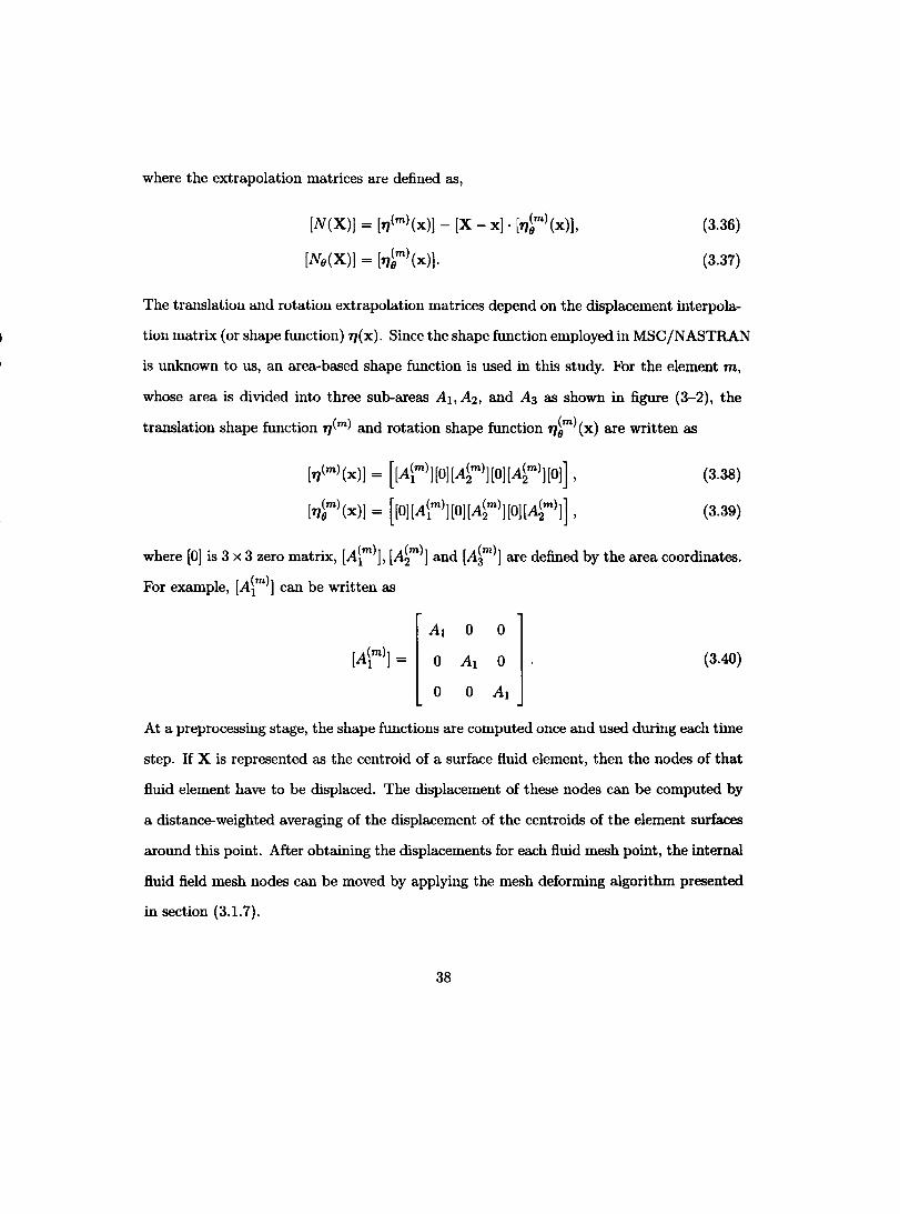
where the extrapolation matrices are defined as,

[N(X)] = [71(m)(x)] - [X - x] . [71~m)(x)],

[Nl/(X)] = [71~m)(x)].

(3.36)

(3.37)

The translation and rotation extrapolation matrices depend on the displacement interpola-

tion matrix (or shape function) 71(X). Since the shape function employed in MSC/NASTRAN

is unknown to us, an area-based shape function is used in this study. For the element m,

whose area is divided into three sub-areas Al. A2, and A3 as shown in figure (3-2), the

translation shape function 71(m) and rotation shape function 71~m)(X) are written as

[71(m)(x)] = [[A~m)][O][A~m)][O][A~m)][O]] ,

[71~m)(X)] = [[O][A~m)][O][A~m)][O][A~m)]] ,

(3.38)

(3.39)

where [0] is 3 x 3 zero matrix, [A~m)], [A~m)] and [A~m)] are defined by the area coordinates.

For example, [A~m)] can be written as

Al 0 0

o Al 0

o 0 Al

(3.40)

At a preprocessing stage, the shape fuIlctions are computed once and used during each time

step. If X is represented as the centroid of a surface fluid element, then the nodes of that

fluid element have to be displaced. The displacement of these nodes can be computed by

a distance-weighted averaging of the displacement of the centroids of the element surfaces

around this point. After obtaining the displacements for each fluid mesh point, the internai

fluid field mesh nodes can be moved by applying the mesh deforming algorithm presented

in section (3.1.7).

38

3.3.2 Load Transfer

The load can be transfered from fluid mesh points to finite element nodes, in a similar

manner, in which the displacement was transfered from the finite element nodes to fluid

mesh points. The transfer of loads algorithm must observe the conservation of loads and

energy principles. If f is external force vector acting on the structural nodes and 8q denotes

the displacement vector, then,

f . 8q = r p8udS, Jav (3.41)

where p is the pressure on the fluid element and S is the product of the normal vector

and the area of the fluid element. Substitute equation (3.34) and discretize the integral to

yield,

(3.42)

for each structural element, we can write

(3.43)

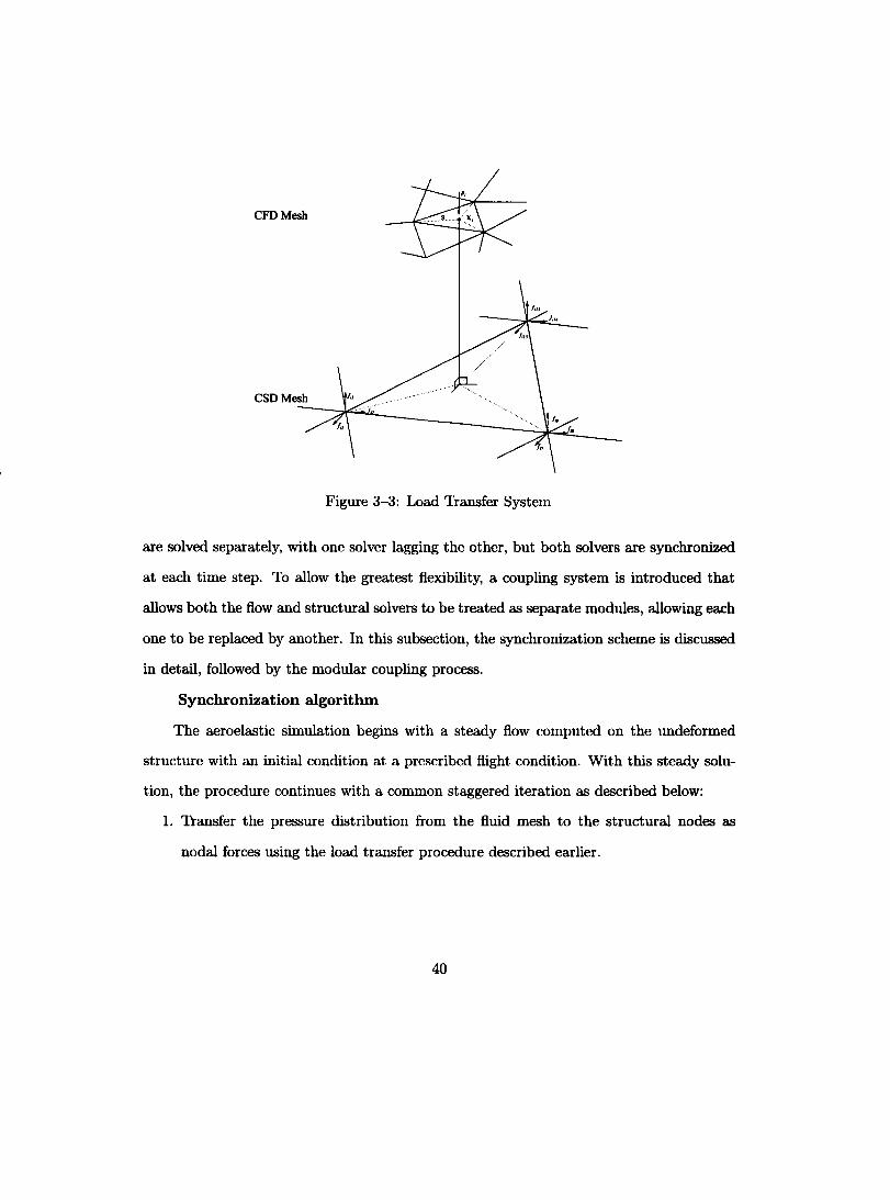
where fi is the nodal force vector. The components fi at each element node are shown

in Figure (3-3). Summing up the components of fi at every structural node gives the

transfered force at that node. By summing up the forces acting on the structural nodes,

(3.44)

we can validate that this force transfer satisfies conservation of load and energy.

3.3.3 Coupling Procedure

The fluid and structural solvers, as described in the previous sections, have been de-

veloped with difIerent numerical methods. An ideal computational aeroelastic simulation,

would require the simultaneous solution of both solvers at each time step. However, this ap­

proach is both computationally challenging and costly. Therefore, in this work both solvers

39

CFDMesh

Figure 3-3: LoOO Transfer System

are solved separately, with one solver lagging the other, but both solvers are synchronized

at each time step. To allow the greatest flexibility, a coupling system is introduced that

allows both the flow and structural solvers to be treated as separate modules, allowing each

one to be replaced by another. In this subsection, the synchronization scheme is discussed

in detail, followed by the modular coupling process.

Synchronization algorithm

The aeroelastic simulation begins with a steOOy flow computed on the undeformed

structure with an initial condition at a prescribed flight condition. With this steOOy solu­

tion, the procedure continues with a common staggered iteration as described below:

1. Transfer the pressure distribution from the fluid mesh to the structural nodes as

nodal forces using the 1000 transfer procedure described earlier.

40

2. Advance the structural equation of motion with the ,6-Newmark method using the

stored displacements at time steps (n - 1) and (n - 2) and the 1000s at n, (n - 1),

(n - 2) to acquire the displacement at the nth time step.

3. Transfer the displacements from the structural nodes to the fluid element centroids

using the displacement transfer algorithm. Perturb the surface fluid nodes based on

the displacements at the fluid centroid.

4. Advance the fluid equations to obtain the pressure distribution for the nth time step

using the stored displacements and flow field at the (n - 1) and (n - 2) time steps.

Steps (1 '" 4) are repeated until the expected time history of the solution are ac­

quired. The resolve and attain the desired simulation, the time step used for both the

flow and structural solvers are of primary importance. Flow solvers generally require small

time steps, limited due to both the need to resolve important flow features and stability

restrictions of the scheme. Structural solvers, however, have no time step limitations.

Figure (3-4) illustrates two common synchronization schemes. The first describes a

simple scheme, where the 1000 is transfered from the flow solver to the structural solve

at the beginning of the time step. The structural solver then OOvances one time step and

provides the flow solver with new displacements. The flow solver, then performs several

Newton iterations to arrive at a converged solution. If too large of a time step is used, the

system cau become unstable, since either the structural solver or the flow solver lags the

other. To prevent inaccurate results due to lagging, very small time steps can be utilized,

however, this approach can have an undesirable effect on the computational cost.

In the second scheme, which is employed in this work, the 1000 is trausfered at the

beginning of the time step. The structural solver than OOvances a provides new displace­

ments. Based on the new surface displacements, the flow solver performs several Newton

iterations. The flow solver then, provides the structural solver with new loads and the

41

w" @

W"+I Fluid

CD b 4~~ [ 4~~ E. ë ~ ë

op~ ~ClJt ~lJt

ri> ,~~ ri> ~,fr. ;- ;-.. .. e~

Structure

'1" @ '1"+1

Before Modification

w" @

w"+1 Fluid

CD

Structure

After Modification (Adding sub-iterations)

Figure 3-4: Synchronization Scheme

structural solver repeats the same time step with the new loads. The flow solver, then

repeats the time step based on these new displacements. A repetition of the time step

is defined as a sub-iteration (or coupling instance). Typically two to three sub-iterations

were used in this study. At each sub-iteration, three Newton iterations were used for the

flow solver, which may not be sufficient to pro duce a converged solution. However, since a

couple of sub-iterations are used during the entire time step, the total number of Newton

iterations will eventually produce a converged solution. The advantage of sub-iterations is

that it prevents lagging and allows for larger time steps.

42

FSCOUPLE

FENSAP

Figure 3-5: Schematic of Modular Coupling System for Node-to-element Approach

Modular Fluid-Structure Coupling

The fluid-structure coupling employs a modular form as shown in Figure (3-5). It

consists of four modules: flow solver (FENSAP), structural solver (MSN/NASTRAN),

preprocessor (FSPREPROC), and coupling controller (FSCOUPLE). Apart from the flow

and structural solvers that have been described earlier, the preprocessor and coupling

controller are essential to acquiring aeroelastic solutions.

The preprocessor has two primary functions: first, read the current flow solution and

transfer pressure distribution from fluid mesh to structural nodes (Load Transfer AIgo­

rithm)j second, read structural displacements and transfer displacement vector to fluid

surface nodes.

The coupling controller is responsible for enforcing the synchronization scheme de­

scribed above. FSCOUPLE achieves this by using TCP /IP sockets for inter-pro cess com­

munication between the modules. This pro cess typically functions as follows: first, the

separate modules (clients) are launched. Each module, binds to a TCP /IP port on the

43

local host; second, the FSCOUPLE code (server) is launched and the software binds to the

ports for each module.

Once the connection between the server and the three clients are established, the syn­

chronization scheme is implemented by the server sending signals to the clients to either

start or stop a process. When a client has completed its task, such as FSPREPROC suc­

cessfully transferring the loads to the structural solver, it sends a signal to the server. Loads

and dis placements are transfered between modules through files. In the future, the loads

and displacements will be transfered through the sockets, thereby reducing communication

time.

44

CHAPTER4 Isogai Test Case

The chapter presents aeroelastic simulations of a sweptback wing section model. Flut­

ter solutions for subsouic and transonic flows are calculated, and a complete trausonic

flutter bouudary is presented.

4.1 Physical Model

To accurately portray the observed dynamic behavior of sweptback wings, lsogai [29]

carefully chose the structural parameters of this model by examining its responses to small

perturbations. The result was that the elastic axis was placed a semi-chord length ahead of

the leading edge of the airfoil and the ratio of uucoupled natural frequency in pluuging and

pitch was set to 1. This case has been numerically investigated by several researches [13,

30, 1, 49] with the following structural parameters,

a - 2, position of elastic axis, from mid-chord, in uuits of semi-chord length b,

f..L 60.0,

XQ 1.8,

r 2 Cl< 3.48,

Wh 1 =

WQ

ln the present study, the semichord length,b is 0.5 m, and the pluuging natural frequency

Wh is 100 rad/s. The shape of the airfoil is that of a NACA64AOlO (NASA Ames model

10.6% thick with a pointed trailing edge [11], comparing with the analytical model with a

squared trailing edge).

45

4.2 Mesh Generation

FENSAP is a 3-D unsteady Navier-Stokes flow solver. 2-D problems are solved by

extruding the 2-D domain in the wing span direction and imposing symmetric boundary

conditions on the symmetric planes. The mesh used in FENSAP is generated in the domain

enclosed by these two symmetric planes, the far-field and the wing surface. The far-field

is placed 20 chord lengths from the wing surface.

In the present study, two hexa meshes are generated to study the effects of mesh

resolution on the solution. The first, designated as 'General Mesh' will be used for the

majority of the calculations to be presented in the following sections. The second, labeled

as 'Transonic Mesh' is similar to the initial mesh but with a finer mesh resolution or higher

density in the vicinity of the shock wave which is present at transonic speeds. The hexa

meshes are created by generating a 2-D hexahedral C-mesh on one of the two symmetric

boundary surfaces and extruding it to the other symmetric boundary surface. More details

of the hexa meshes will be provided in subsequent sections.

4.3 Numerical Setup

To illustrate the complete flutter boundary, flutter points are calculated at Mach

numbers 0.7, 0.825, 0.85, 0.875, and 0.88. The complete procedure to compute a flutter

point, is as follows:

1. Compute the steady-state solution at the given free-stream Mach number Mao, free­

stream density Pao, and temperature Tao at zero angle of attack. Employ mesh

adaptation to optimize the mesh for the given flight condition.

2. Compute an initial unsteady solution by forcing the motion of the airfoil for three

cycles of oscillation at the frequency of the plunging mode between ± 10 angle of

attack.

46

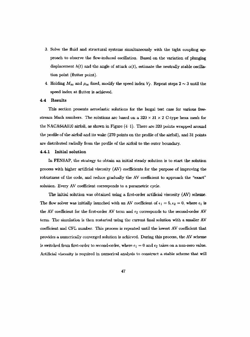
3. Solve the Huid and structural systems simultaneously with the tight coupling ap­

proach to observe the How-induced oscillation. Based on the variation of plunging

displacement h(t) and the angle of attack a(t), estimate the neutrally stable oscilla­

tion point (Hutter point).

4. Holding Moo and Poo fixed, modify the speed index VI' Repeat steps 2 '" 3 until the

speed index at Hutter is achieved.

4.4 Results

This section presents aeroelastic solutions for the Isogai test case for various free­

stream Mach numbers. The solutions are based on a 320 x 31 x 2 C-type hexa mesh for

the NACA64AOlO airfoil, as shown in Figure (4-1). There are 320 points wrapped around

the profile ofthe airfoil and its wake (270 points on the profile of the airfoil), and 31 points

are distributed radially from the profile of the airfoil to the outer boundary.

4.4.1 Initial solution

In FENSAP, the strategy to obtain an initial steady solution is to start the solution

pro cess with higher artificial viscosity (AV) coefficients for the purpose of improving the

robustness of the code, and reduce gradually the AV coefficient to approach the "exact"

solution. Every AV coefficient corresponds to a parametric cycle.

The initial solution was obtained using a fust-order artificial viscosity (AV) scheme.

The How solver was initially launched with an AV coefficient of q = 5, f2 = 0, where fI is

the AV coefficient for the first-order AV tenn and f2 corresponds to the second-order AV

term. The simulation is then restarted using the current final solution with a smaller AV

coefficient and CFL nwnber. This process is repeated until the lowest AV coefficient that

provides a numerically converged solution is achieved. During this process, the AV scheme

is switched from fust-order to second-order, where q = 0 and f2 takes on a non-zero value.

Artificial viscosity is required in numerical analysis to construct a stable scheme that will

47

(a) Overview of Grid

(h) Close-up View

Figure 4-1: C-type Hexa Mesh for NACA64AOlO airfoil. 320 x 31 x 2

48

guarantee convergence. However, if the contribution from AV is too large, it will have a

negative impact on the quality of the solution. Therefore, the contribution from AV should

be the lowest possible to achieve a converged solution. In this work, the final simulation

was obtained with an AV coefficient of €2 = 0.02 for subsonic case. For transonic test

cases, the second-order AV scheme with shock sensor is used for its ability to reduce to a

fust-order scheme at the shock and second-order elsewhere. The AV coefficient € is set to

0.004 for both the fust-order and second-order term [3]. In each case, the artificial viscosity

is lowered gradually in parametric cycles until a divergent solution appears. This approach

guarantees the best available initial solution to launch an unsteady ca1culation.

Figure (4-2) illustrates the convergence of the residual for a steady inviscid transonic

flow at Mach 0.825. Five parametric cycles were employed with each designated to an

AV scheme with a predefined AV coefficient. The spikes indicate that the AV coefficient

has been lowered. The residual usually increases when the coefficient is lowered but will

eventually reduce. The last spike in the residual corresponds to the final computation with

the lowest AV coefficient. This simulation required several thousand iteratiollS to achieve

a machine zero convergence.

Figures (4-3)a and (4-3)b illustrate the pressure distribution at Moo = 0.7 and Moo =

0.825. The solution was obtained at a zero angle of attack. Figure (4-3)b demonstrates

the presence of a shock wave on both the upper and lower surfaces. Figures (4-3)c and

(4-3)d illustrate the respective Mach contours. The convergence of the contour lines in the

later plot, signifies the location and strength of the shock wave.

4.4.2 Pitching Airfoil

The code and grid are validated by forcing the wing section to pitch around its quarter

chord. The lift coefficient versus angle of attack is compared with the experimental NACA

64AOIO CT6 [11] data. Here the computations are performed at the freestream Mach 0.796,

49

10'" r---,.----r---,-----r----r---,------r-----,

10-'O'-----'----'--_-'--_---' __ --'-__ -'--_---' __ -.J o 1000 2000 3000 4000 5000 6000 7000 6000

Tlme Slap N

Figure 4-2: Residuals for the Steady Inviscid Transonic Flow (Mec = 0.825)

at a mean angle of attack ao = 0°, with a maximum angle of attack am = 1.01°, and a

reduced frequency Wr = 0.202. A minimum of five cycles of computation are required in

order for the periodic steady state flow to be established, and allow the time-accurate lift

and moment coefficients to converge. Figure (4--4)a-d show the hysteresis loop, the CT6

experimental results and the evolution of Cl and Cm in time. The coefficient of lift hysteresis

loop compares weIl with the experimental data for an inviscid simulation. The coefficient

of moment provides the correct trend, but the magnitudes of the moment coefficients do

not compare weIl with experimental values. One reason for the discrepancy between the

computational and experimental moment coefficient may be due to the fact that only an

inviscid model is considered in these testcases. Accurate moment coefficients require accu-

rate representation of the pressure distribution at the trailing edge which is only possible if

viscous terms are included. Nevertheless, the aeroelastic solutions based on these moment

50

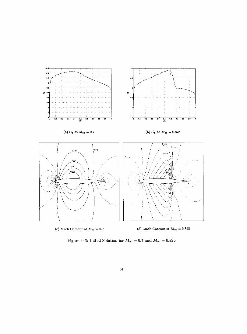
-<1.2

0.2

8" 0.4

./

0.6

0.6

1.2

1.4~0 ----:o:':.1-~O'2:---:'0.3:----=0 .. ';---:0'7.5 ----:0:'::.6-0~.7:---:'0.8:----=0.-:-9 -----.l JI.

(a) Cp at Moo = 0.7

(c) Mach Contour at Moo = 0.7

-<1.5

0.5

~ ~ U M ~ M M UMM JI.

(b) Cp at Moo = 0.825

(d) Mach Contour at Moo = 0.825

Figure 4-3: Initial Solution for Moo = 0.7 and Moo = 0.825

51

coefficients were able to provide a flutter boundary curve that compares well with other

numerical data.

The Mach contour and Cp distribution at every quarter of the period are illustrated

in figure (4-5) and (4-6). The figures demonstrate the movement of the shock wave as

the airfoi! undergoes a pitching motion. The accurate capture of the location of the shock

wave is important for aeroelastic simulations.

4.4.3 Aeroelastic Simulation

To obtain an aeroelastic simulation, a forced oscillation for three periods was ini­

tially used to eliminate transient solutions and most importantly to excite the fundamental

modes of vibration. After three periods of forced oscillation, the Fluid-Structure Interface

is started and the displacements are no longer prescribed but computed based on the struc­

tural equations of motion. The simulation is run for several time steps until either a stable,

neutrally stable, or unstable response is computed.

In the following computations, the flow simulation is based on an inviscid solution, and

at an artificial viscosity level that is similar to the value used to obtain the initial solution.

At each time step, two sub-iterations were performed, with a maximum of three Newton

iterations per sub-iteration. A convergence criteria is also established. Often during the

second sub-iteration, only one or two Newton iterations are used, if the convergence level

satisfies the criteria. The simulations were computed on a SGI Origin 3800 shared memory

machine and generally required a wall clock time of ten hours on 12 processors.

Unsteady calculation at Moo = 0.825

Figures (4-7)a-b illustrates the convergence of the flow solver at each time step. Fig­

ures (4-7a) shows the convergence from the initial condition upto 200 time steps and figure

(4-7)b illustrates the convergence of the fiow solver, when the aeroelastic simulation bas

reached a periodic steady state solution. The simulation was computed at a Mach number

52

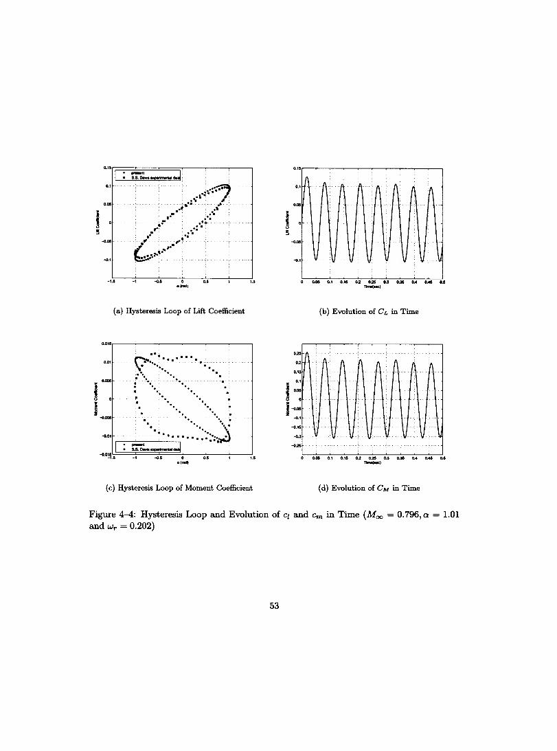
1 '5

1 1

0.1·rr==:===:::;:===='--~--~-1

~~~J 0.1

0.00

-0.00

-0..1

.. \~.:.:~. ,.. 1 . .... ~ . :..... .. '

,6 .\!: .- : .'. 1- .' • . - ..... . . . " .'. . . .

" '. b· .~ , .. "..

.-.. ,." ......

-1 -o. .. o 0" a (Nd,

(a) Hysteresis Loop of Lift Coefficient

t.'

0.01.r-----~--~--~--~-__,

0.01

0.000

., ~

.. . ... .... . . . . •... . ..... . .. ~. ~~~'.. ..... , ... .. . '.. . ................. < .. .'

-0..000

-0.01

. ..... '.... . ... " •••• w •• • ::.:.: ••.•••• "~

••• ..:J ,1 ~00.i0~..J.

-O'~~ .. ~===-~t====~-o.~ .• ====~o~--o~ .• ~-~-~t .. 0(*)

(c) Hysteresis Loop of Moment Coefficient

1 ~

0.15

0.1

0.00

-0..00

-o.t

0.25

0.2

0.15

O.t

1 0.00

o

1-0.·00

-o..t -0.15

-0..2

-0..25

fi f\ A 1\ f\ 1\ fi fi

1

V V V V V V V \J

~ ~ ~ ~ ~ U ~ ~ ~ U ,-Mel

(b) Evolution of CL in Time

~ ~ ~ ~ ~ u ~ ~ ~ U '-Mel

(d) Evolution of CM in Time

Figure 4-4: Hysteresis Loop and Evolution of Ci and Cm in Time (Moo = 0.796, Cl: 1.01 and Wr = 0.202)

53

/ /

\ \

/-

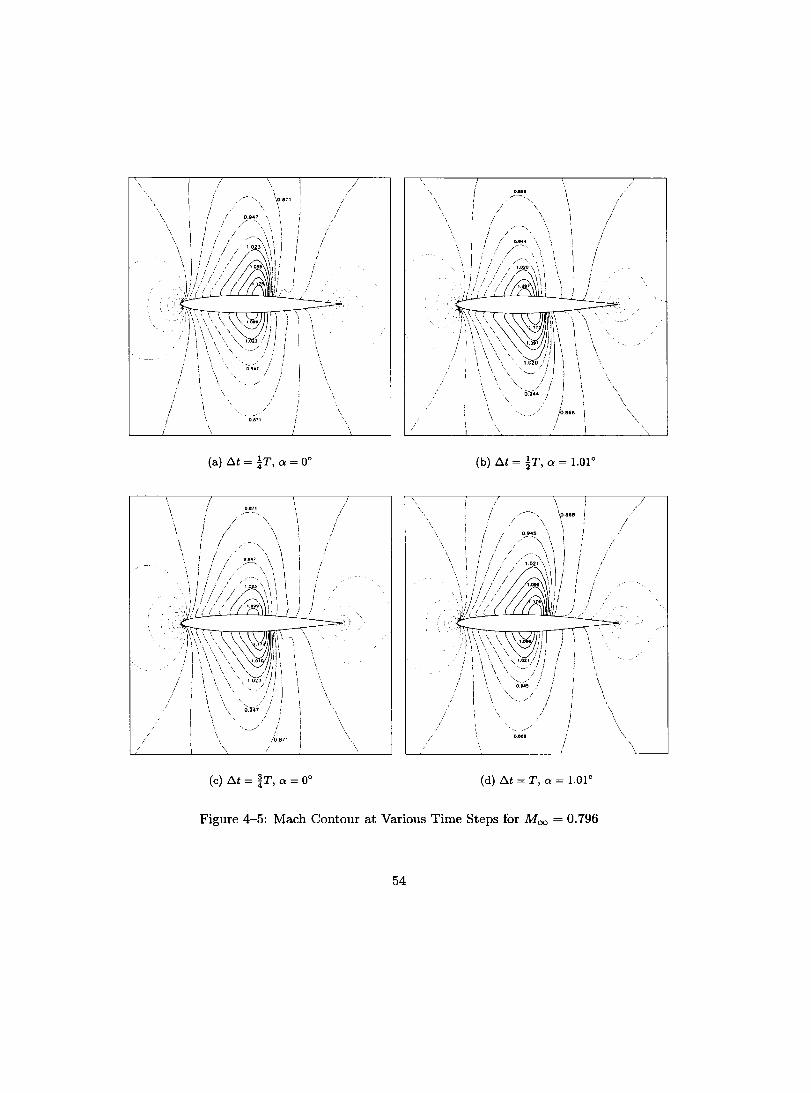
, 0_947 \ ,/ ...... '

! /

(a) f::J..t = ~T, Q = 00

:0,871

(c) f::J..t = ~T, Q = 00

\

/ \

i

f i

0.8IIa .---,

1

! /0.868

!

(h) f::J..t = ~T, Q = 1.010

1 !

,

1 /

(d) f::J..t = T, Q = 1.010

Figure 4-5: Mach Contour at Various Time Steps for Moo = 0.796

54

\

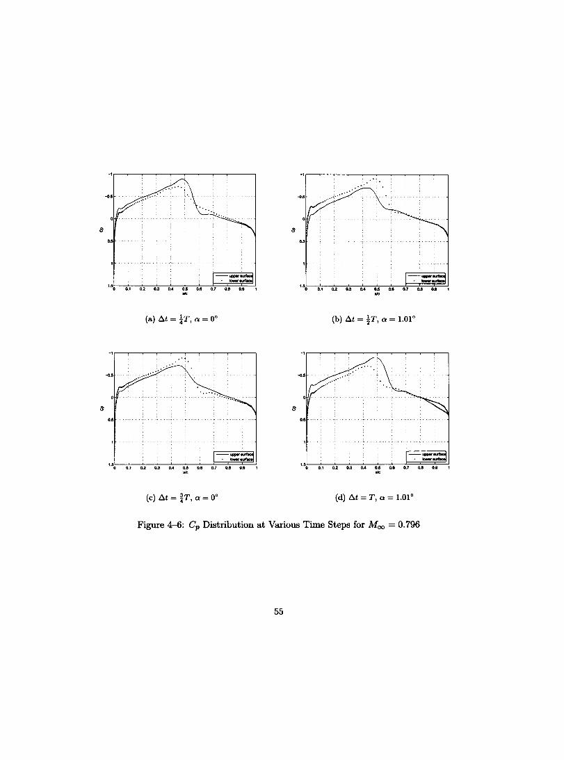
(a) l:l.t = tT, a = 00 (b) l:l.t = ~T, a = 1.010

... -0.5 p ......... .

o

0.5

(c) l:l.t = ~T, a = 00 (d) l:l.t = T, a = 1.010

Figure 4-6: Cp Distribution at Various Time Steps for Moo = 0.796

55

of 0.825 and a speed index, VI = 0.682. The Cp distribution and Mach contours are shown

in figures (4-8) and (4-9).

Aeroelasticity solution

The plunging and pitching responses of the airfoil are shown in figures (4-10 rv 4-18)

at various Mach numbers and speed index. Compared with the response at transonic flow,

the structure in the subsonic flow is more sensitive to the speed index. For instance, the

flutter point speed index for Mach 0.7 is 1.23, when the speed index was changed to a

slightly higher value of 1.30, the response of the airfoil diverged rapidly as shown in Figure

(4-11). For transonic flow, however, the transition from stable to diverged response is not

as abrupt due to the nonlinear effect at this speed range. Figure (4-14) shows the response

at Mach number 0.825 and of the speed index 0.682. For the indexes less then 0.682 the

response is clearly stable as shown in Figure (4-13) and the response damped until the

structure restored to its initial position.

To obtain a periodic steady state solution for the neutrally stable responses, several

periods in the order of 10 to 15 were used, as demonstrated in figures (4-11), (4-14), and

(4-17). This is necessary to eliminate initial transient solutions that appear as spikes and

often persist for three to five periods after the forced oscillation is replaced by the structural

equations of motions.

Flutter Boundary

The flutter boundary can be determined by finding the neutrally stable solution at

various Mach numbers. Figure (4-19) shows the present results and those of Ref. [1,30, 49J.

The results predict the transonic-dip fairly well. As the Mach number approaches unit y,

the flutter speed index dips for a small range of Mach numbers. The present solver obtained

the bottom of "transonic dip" at a speed index 0.52 at Mach number 0.875, and is within

5% compared to other results.

56

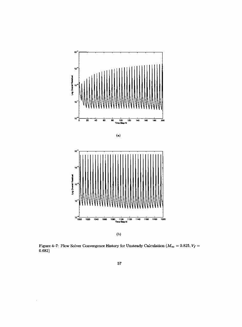
la"

10"L---~--~--~--~--~--~--~--~--~~ o 20 40 60 60 100 120 140 160 160 200

T1meSIopN

(a)

10"L-__ ~ __ ~ __ ~ __ ,--__ ,--__ ,--__ ~ __ ,--__ ,------l 1000 1020 1040 1060 1060 1100 1120 1140 1160 1160 1200

T .... SIopN

(b)

Figure 4-7: Flow Solver Convergence History for Unsteady Calculation (Moo = 0.825, V, =

0.682)

57

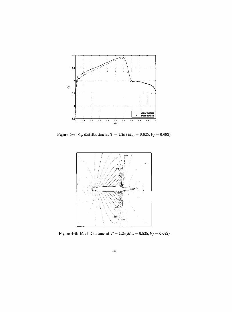
-1r---r---.---.---.----.---r---r--~--~--~

.' .

-0.5 .. ' ,-/ ........ .

o : !

0.5

0.1 0.2 0.3 0.4 0.5 0.6 0.7 0.8 0.9 xie

Figure 4-8: Cp distribution at T = 1.2s (Moo = 0.825, VI = 0.682)

Figure 4-9: Mach Contour at T = 1.2s(Moo = 0.825, VI = 0.682)

58

~ .., c ID

i c

0.02

~ ~ ~ 0.015 .. .. .. .. .. ..

0.01

0.005 , ,

of--_...J

r===hibl -~

..

.~ -0.005 .... ".' ~ " ..

J 11.

-0.01 ... ,. ' .....

-0.015

i i i

-o.020'-----0 ..... 2----0'-.4---0 ..... 6----0'-.8---..J......----'1.2

Time(s)

Figure 4-10: Damped Stable Response (Moo = 0.7, VI = 1.20)

~

0.02r-----r----.----.-------,.------r..:.

I==. =hlba~1

~ ~ ~ 0.015 ::

.. 0.01 .:

i 0.005

i I!! ot---~

1 r -0.005

1 -0.01 .. ' ' ..... ,:.

: : -0.015

ï i ï

-0.020'-----0 ..... 2,----...,0'-.4---0 ..... 6,-----0'-.8----'-----:'1.2

Time(s)

Figure 4-11: Neutra! Stable Response (Moo = 0.7, VI = 1.23)

59

DI .Si 2' .01 IL

0.04 r------r----.-------r-----r------,r------,

Cl 0.03 ......... -

..

V V V -0.02

-0.03

-o.04~---L---~--~---~--~~--~ o 0.2 0.4 0.6 0.8 1.2

Tlme(a)

Figure 4-12: Divergent Response (Mao = 0.7, VI = 1.30)

: : : : -0.01

..

V V V -0.02

-o.030~---0.L.2---0..L.4---0:-'-.6---0...J..8.,------'------'1.2

Tlme(a)

Figure 4-13: Damped Response (Mao = 0.825, VI = 0.66)

60

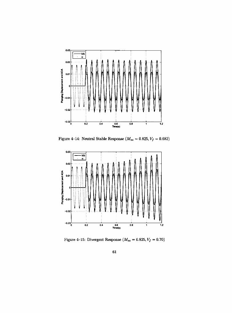
O.03,-----.------r---....-------r---.--------,

El 0.02 .. -

.-

v V V -0.02

-o.030L----0.L2-----J0.-4 -----l0.6---0....l..8---..I....---......J

1.2

Time(s)

Figure 4-14: Neutral Stable Response (Moo = 0.825, VI = 0.682)

0.03.-----,------r---....-------r---.---.----,

El 0.02

-< ~ ~ ~ ~ 1 0.01

j ol---....J

1

: :

r : : •

!!' -0.01

t. V V V

-0.02

0.2

...

0.4 0.6 Tome(s)

0.6 1.2

Figure 4-15: Divergent Response (Moo = 0.825, VI = 0.70)

61

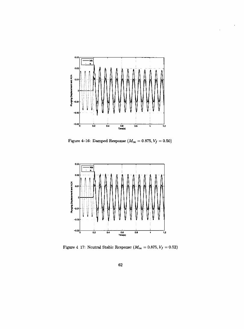
o.03r===::r----.-----,----,.-----,r-------,

EJ 0.02

g §' -0.01 iL

..

V v V -0.02

-o·030~--O~2~-~0.~4--~0~~--~0.8---~-~12 Tme(a)

Figure 4-16: Damped Response (Moo = 0.875, VI = 0.50)

O.03r----,-----.-----,----,.------,r-------,

0.02

~ ~

~ t\ ~ ~ i 0.01

lot------'· . . . . i! .~ ~ -0.01 iL

-0.02

-o·030L---0~2~-~0.~4---0~.8---0~~---~-~12

Time(o)

Figure 4-17: Neutra! Stable Response (Moo = 0.875, VI = 0.52)

62

O.03r----r------,----,-----r------,------,

El 0.02

~ ft oC 1 0.01

i !!' 1-0·01

V V V -0.02

-o·030~--~02~--O~A--~O~.8--~OB---~--~12

Time(.)

Figure 4-18: Divergent Response (Mao = 0.875, V, = 0.54)

3

2.5

2

:> )( v -8 .5 1.5

1 III

0.5

OL---~----~----~--~----~----~--~-----" ~ ~ ~ v ~ ~ ~ M ~

Mach Number

Figure 4-19: Flutter Boundary (VI = w5?1t)

63

4.4.4 Effect of High-density Region

In the present study, a general mesh, as shown in figure (4-1), without a high-density

region in the vicinity of the shock wave was used for all test cases. The flow solver was able

to capture the shock wave on this mesh for various Mach numbers. However, a transonic

mesh with a finer mesh resolution in the neighborhood of the flow discontinuity would be

able to locate the shock wave with a higher precision. The finer mesh contains approxi­

mately 36,000 nodes compared to 19,800 for the general mesh. Figure (4-20) illustrates a

comparison of the pressure and Mach number distribution obtained from the two meshes

and a close-up view of the transonic mesh. The pressure distribution illustrates that both

grids were able to agree well on the location of the shock. However, for the general mesh,

the flow discontinuity is smeared over a larger number of mesh points, but the transonic

mesh produced a 'sharper' discontinuity as shown in figure (4-20)c.

Figures (4-21) and (4-22), demonstrate the aeroelastic response at a Mach number of

0.825. The fust figure illustrates a neutrally stable response and the second an unstable

response. If figure (4-21) is compared to figure (4-14) a difference between the responses

can be observed. The simulation using the general mesh was obtained at a speed index of

0.682 and for the transonic mesh at a value of 0.684. The difference between the speed index

is only 0.3%, however, the amplitudes of the pit ching angles and plunging displacements are

dissimilar. This difference is due mainly to the difference between the pressure distributions

observed in figure (4-20) between the two grids. The disparate pressure plots can lead to

differences to both the lift and moment coefficients, causing a slightly different aeroelastic

response. This test, demonstrates the importance of mesh quality. Both grids were able

to predict an accurate flutter point, however, the finer mesh was able to provide more

accurate displacements.

64

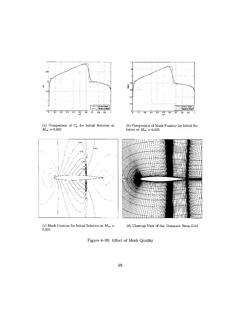
-lr--~-~-~~-~-~-r--~-~---,

o .•

1.50 0.1 0.2 0.3 0.4 0.5 0.6 0.7 >le

(a) Comparison of Cp for Initial Solution at Moo = 0.825

(c) Mach Contour for Initial Solution at Moo = 0.825

o .•

0.2

l _._ .... ~=:::~ 0~0-~0.1~~0~.2~0~.3~~0.~.~0~ .• -706~~0~.7==O~.8~~0.~.~

>Je

(b) Comparison of Mach Number for Initial So­lution at Moo = 0.825

(d) Close-up View of the Transonic Hexa Grid

Figure 4-20: Effect of Mesh Quality

65

o.o3r----,-----,----r---~---.,__--__,

~ 0.02

« ~ ~ ." 0.01 5i

i 0

J .....

.~ : : : : ~ -0.01

f. V V V

-0.02

-o.030~---:'0.':-2 ------'0.4---0...1..6:----0=-'-.8----'-----'1.2

Tme(a)

Figure 4-21: Neutral Stable Response with Transonic Mesh (Moo = 0.825, VI = 0.684)

O.03.-----r-----,----r---~---.,__--__,

0.02

~ ~

A ~ ." 0.01 5i

i J '" ~ .O! Q.

o t--.. -.-.-........

-0.01 ..

V V V -0.02

-0.03l...----'------'----'---------'-----'-----' o 0.2 0.4 0.6 0.8 1.2

Tme(s)

Figure 4-22: Divergent Response with Transonic Mesh(Moo = 0.825, VI = 0.70)

66

4.4.5 Effect of Coupling Time Step

To achieve proper temporal resolution, a temporal convergence study is presented in

this subsection. The time step is determined by at = w~~N' where N is the number of time

steps per period. Figure (4-23) and (4-24), show the effect of N on the response of airfoil

at Mao = 0.825 and a speed index VI = 0.682. As illustrated, the solution converges for

N greater than and equal to 100. The results presented in the previous subsections were

obtained with 100 time steps per period. There is no observable difference between the

solutions obtained for 100 or 400 time steps per period. However, at N = 50 the aeroelastic

response obtained is that of a damped response. A smaller N value corresponds to a larger

time step, at. A large time step introduces additional numerical damping, which has the

similar effect of having viscous damping. The overall effect is an over prediction of the

flutter point.

4.4.6 Effect of Number of Sub-Iterations

Figure 4-25 illustrates the aeroelastic response due to the number of sub-iterations.

Performing two sub-iterations per time step allows both the flow and structural solvers to

repeat the time step based on the latest data. For the case of two and three sub-iterations,

the solutions are approximately equivalent. However, for the case of a single iteration, the

aeroelastic simulation results to an unstable response. Either the flow solver or structural

solver always lags the other. The number of Newton iterations for the flow solver per

sub-iteration was kept constant for all three cases.

67

0·03rr==~~---.----.----r---"---1

I -_~:~ool --N=4001 0.02

~ 0.01

1 ot----' CI .S;

1-0.01

c

~

-0.02

-o·030L------0.~2------0.~4------0.~6------0.~6------L-----~1.2

Tlme(s)

0.01

0

-0.01

-0.02

-0.03 0 0.2

(a) Plunge Displacement

0.4 0.6 TII11II(I)

0.8

(h) Angle of Attack

1.2

Figure 4-23: Eflect of Non Aeroelastic Response (Moo = 0.825, VI = 0.682)

68

~ 0.01

1 0.005

! 0

.!!' -0.005 I!' ::> i5: -0.01

-0.015

-0.02

-0.0251 1.02 1.1 1.12 1.14 1.16 1.2

TIme(a)

(a) Plunge Displacement

-O.D15L--"----'----'---'---'----'------'.----'----''-----.J 1 1.02 1.04 1.06 1.06 1.1 1.12 1.14 1.16 1.18 1.2

Tome(a)

(h) Angle of Attack

Figure 4-24: Close-up View of the Effect of Non Aeroelastic Response (Moo = 0.825, V, = 0.682)

69

S

~

0.05rr==:::r::==:::::r::;~----'--.-----'---""'--r-~

0.04 11 _- ~ :::~ rl--3cou~~

0.03

-0.02

-0.03

-0.04

0.2 0.4 0.6 0.8 1.2 1.4 1.6 TlfM(uc)

(8) Plunging Displacement

0.01

0

-0.01

-0.02

-0.03 0 0.2 0.4 0.6 0.8 1.2 1.4 1.6

TlfM(uc)

(b) Angle of Atta.ck

Figure 4-25: Eflect of Number of Sub-Iterations per Time Step. (Moo = 0.825, VI = 0.682)

70

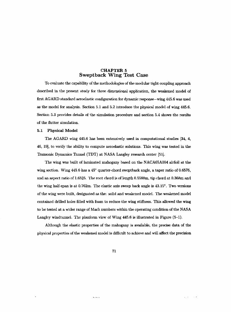
CHAPTER 5 Sweptback Wing Test Case

To evaluate the capability of the methodologies of the modlÙar tight coupling approach

described in the present study for three dimensional application, the weakened model of

first AGARD standard aeroelastic configuration for dynamic response-wing 445.6 was used

as the model for analysis. Section 5.1 and 5.2 introduce the physical model of wing 445.6.

Section 5.3 provides details of the simulation procedure and section 5.4 shows the reslÙts

of the flutter simlÙation.

5.1 Physical Model

The AGARD wing 445.6 has been extensively used in computational studies [34, 4,

46, 19], to verify the ability to compute aeroelastic solutions. This wing was tested in the

Transonic Dynamics Thnnel (TDT) at NASA Langley research center [51).

The wing was built of laminated mahogany based on the NACA65A004 airfoil at the

wing seCtiOll. Wing 445.6 has a 45° quarter-chord sweptback angle, a taper ratio of 0.6576,

and an aspect ratio of 1.6525. The root chord is of length 0.5588m, tip chord at 0.368m and

the wing half-span is at 0.762m. The elastic axis sweep back angle is 43.15°. Two versions

of the wing were built, designated as the: solid and weakened model. The weakened model

contained drilled holes filled with foam to reduce the wing stiffness. This alloWed the wing

to be tested at a wider range of Mach numbers within the operating condition of the NASA

Langley windtunnel. The planform view of Wing 445.6 is illustrated in Figure (5-1).

Although the elastic properties of the mahogany is available, the precise data of the

physical properties of the weakened model is difficlÙt to achieve and will affect the precision

71

Figure 5-1: Planform View of AGARD Wing 445.6

of the numerical simulations of the wing. Based on a 10 x 10 plate element model with

varying thickness, Spain [44] performed a finite element analysis of the weakened model with

MSC/NASTRAN. In the report, the material properties of the wing were: p = 40.33kg/m3 ,

Ex = 3.4497 x 109 N/m2, Ey = 1.03425 X 109 N/m2, G = 0.44818 X 109 N/m2, and v = 0.31,

which were carefully chosen in order to best duplicate as closely as possible to the measured

modal frequencies. The natural frequencies obtained by finite element analysis and by

experiments are listed in Table 5-1. Since both results compare well, the material properties

used in this work are based on Ref. [44].

Table 5-1: Comparison of Natural Frequencies

Mode Spain [44] Yates [51] Present FE analysis First Bending 9.6 9.6 9.61 Second Bending 48.35 50.7 56.70 First Bending 38.17 38.10 37.06 Second Torsion 91.54 98.5 89.42

72

-

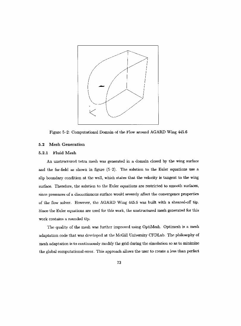
Figure 5-2: Computational Domain of the Flow around AGARD Wing 445.6

5.2 Mesh Generation

5.2.1 Fluid Mesh

An unstructured tetra mesh was generated in a domain closed by the wing surface

and the far-field as shown in figure (5-2). The solution to the Euler equations use a

slip boundary condition at the wall, which states that the velo city is tangent to the wing

surface. Therefore, the solution to the Euler equations are restricted to smooth surfaces,

since presences of a discontinuous surface would severely affect the convergence properties

of the flow solver. However, the AGARD Wing 445.6 was built with a sheared-off tip.

Sillce the Euler equations are used for this work, the ullstructured mesh gellerated for this

work contains a rounded tip.

The quality of the mesh was further improved using OptiMesh. Optimesh is a mesh

adaptation code that was developed at the McGill University CFDLab. The philosophy of

mesh adaptation is to continuously modify the grid during the simulation so as to minimize

the global computational error. This approach allows the user to create a less than perfect

73

grid within a matter of hours and through the mesh adaptation proeess, grid elements

are refined in sorne regions to highlight important flow features and increased in others

where there are negligible change to the local flow field. The strategy of mesh adaptation

developed at the McGill University CFDLab has been demonstrated to be a powerful tool

to improve the quality of the mesh and consequently the convergence and accuracy of

the numerical solutions. The core of this technology is the optimization of the mesh by

equi-distributing the interpolation error over the domain in order to minimize the global

computational error.

In this work, mesh adaptation was only performed for the initial solution and not

during the unsteady simulation. Sinee the simulation is performed at a moderate subsonic

Mach number for an inviscid flow, the critical flow feature is to capture the leading edge

peak pressure accurately. Figures (5-6a-b) illustrate the final mesh generated after three

cycles of mesh adaptation, in particular, figure (5-6b) clearly illustrates that the mesh

adaptation algorithm has increased the number of points near the leading edge to provide

a better resolution of the peak pressure, while elements on the top and bottom surfaces

were coarsen sinee the surface pressure gradient in those regions are rather small. The final

mesh contains 138,620 nodes and 686,059 elements.

In Ullsteady calculation, the mesh deforming algorithm is employed to maintain a

smooth mesh. Figure (5-4) illustrates the continuous surface mesh with no irregularities

before and after surface deflection.

5.2.2 Structural Mesh

The structural wing model is represented by a thin plate, limited by the leading and

trailing edge points of the stream-wise wing sections at the root and wing tip. The model

uses 12 nodes along the stream-wise direction and 20 in the span-wise direction, to produee

a total of 240 nodes. The nodes are equally distributed in both directions. Figure (5-5)

74

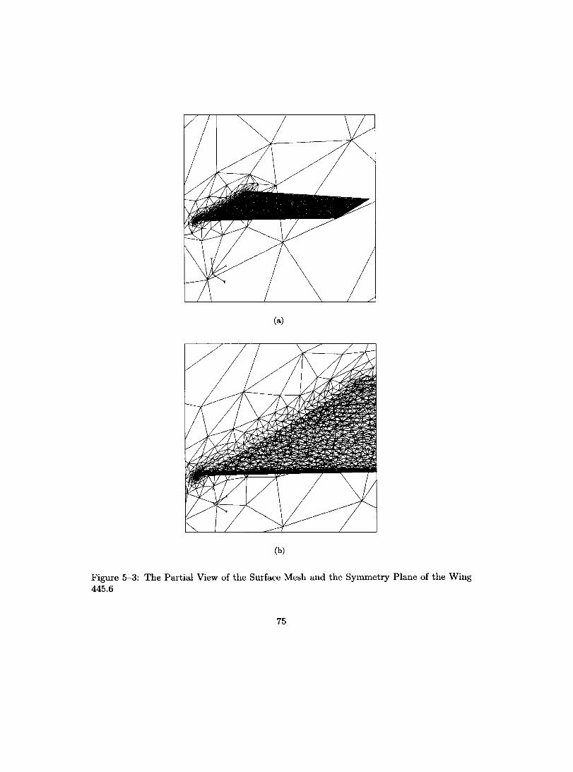
(a)

(h)

Figure 5-3: The Partial View of the Surface Mesh and the Symmetry Plane of the Wing 445.6

75

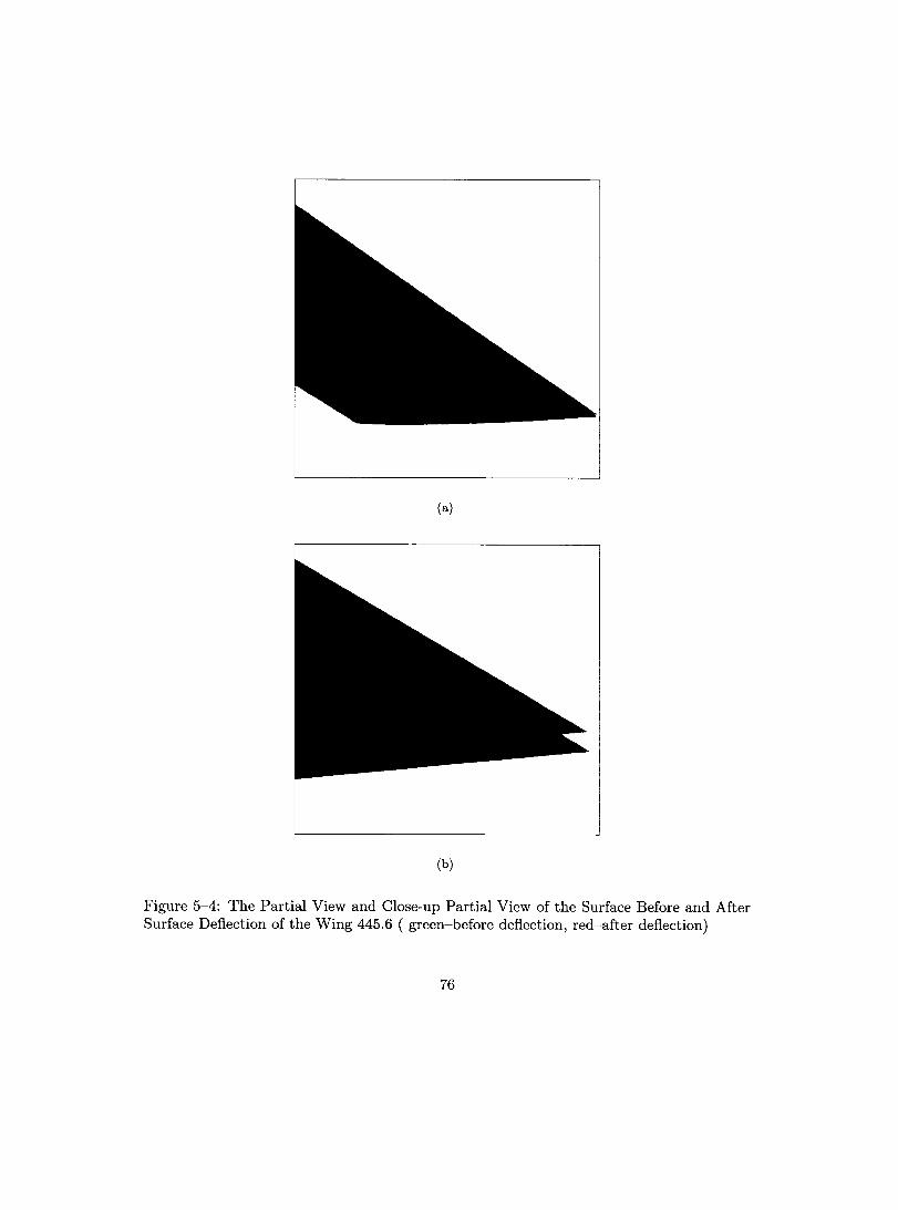
(a)

(b)

Figure 5-4: The Partial View and Close-up Partial View of the Surface Before and After Surface Defiection of the Wing 445.6 ( green-before defiection, red-after deflection)

76

~~ ~~ ~ ~

~ ~~~ '0 f\

f' rof.-

IS.:\~

~ R f' ~

~~~ ""- ~

"\

"< ~ ~

Figure 5-5: The Structural Mesh of Finite Element Model of Wing 445.6

illustrates the finite element structural mesh. The nodes form a triangular element and

are represented in MSC/NASTRAN as CTRIA3 trilateral elements. CTRIA3 allows for

variable thickness elements, by enabling the user to represent the local thickness of the

airfoil section at the structural nodes. The natural frequencies of the structural model

were computed based on the properties of the AGARD weakened Wing 445.6. The modes

of vibration are shown in figure (5-6) and (5-7), where the variational bending and torsional

modes have been identified by plotting the deflection of the wing. These deflections agree

well with the results published in [51].

5.3 Numerical Setup

In the present study, the flutter point at Mach llumber 0.499 is evaluated by coupling

the flow sol ver and the transient response analysis of the structure in an implicit approach.

The procedure to perform the aeroelastic analysis at this Mach number is as following,

77

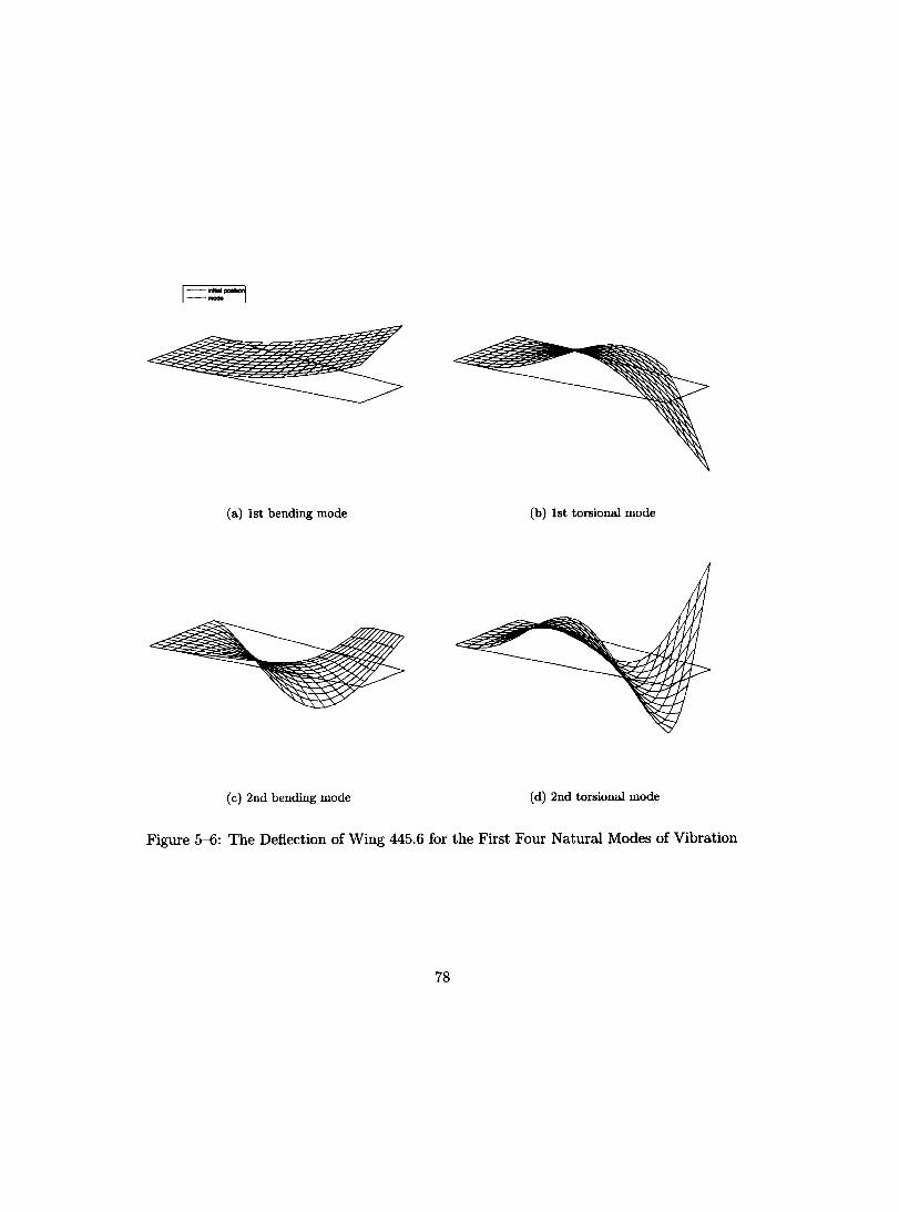
1-:"'4

(a) lst bending mode (b) lst torsional mode

( c) 2nd bending mode (d) 2nd torsional mode

Figure 5-6: The Deflection of Wing 445.6 for the First Four Natural Modes of Vibration

78

(a) lst bending mode (b) lst torsional mode

( c) 2nd bending mode ( d) 2nd torsional mode

Figure 5-7: The Contour of Deflection of Wing 445.6 for the First Four Natural Modes of Vibration

79

1. Obtain the steady-state solution by running flow solver at a freestream Mach number

0.499, temperature Too and pressure POO.

2. Impose a suit able impulse force "dead force" on the mid-chord point of the wing tip

to excite the natural modes of the wing.

3. Solve the flow equations and structural equations simultaneously for several time

steps and observe the displacement of the leading edge and trailing edge of the tip

section. After several time steps, a time history graph of the displacements will

illustrate either a stable, neutrally stable, or unstable response.

4. Keeping Moo and temperature Too constant, vary the free-stream pressure Poo, and

repeat steps 1 '"" 3 until a neutrally stable response is attained.

The following are the flight conditions used for the aeroelastic simulation. The struc­

tural properties are based on the AGARD weakened model.

Il = 33.465, mass ratio, Pwing Vwing / Pair V cone,

Wu = 239.83rad/ sec, natural circular frequency of the first uncoupled torsion mode,

Uoo = 172.456,

pwing = 418.20kg/m3, density of wing,

Pair = 0.4277kg/m3, density of free-stream air (pressure 36485.1Pa),

Vwing = 0.0044531m3, volume of wing,

Vair = O.13054m3 , volume of a truncated right cone enclosing wing,

7rh 2 . 2 = ï2(croot + c,.ootttp + Ctip),

80

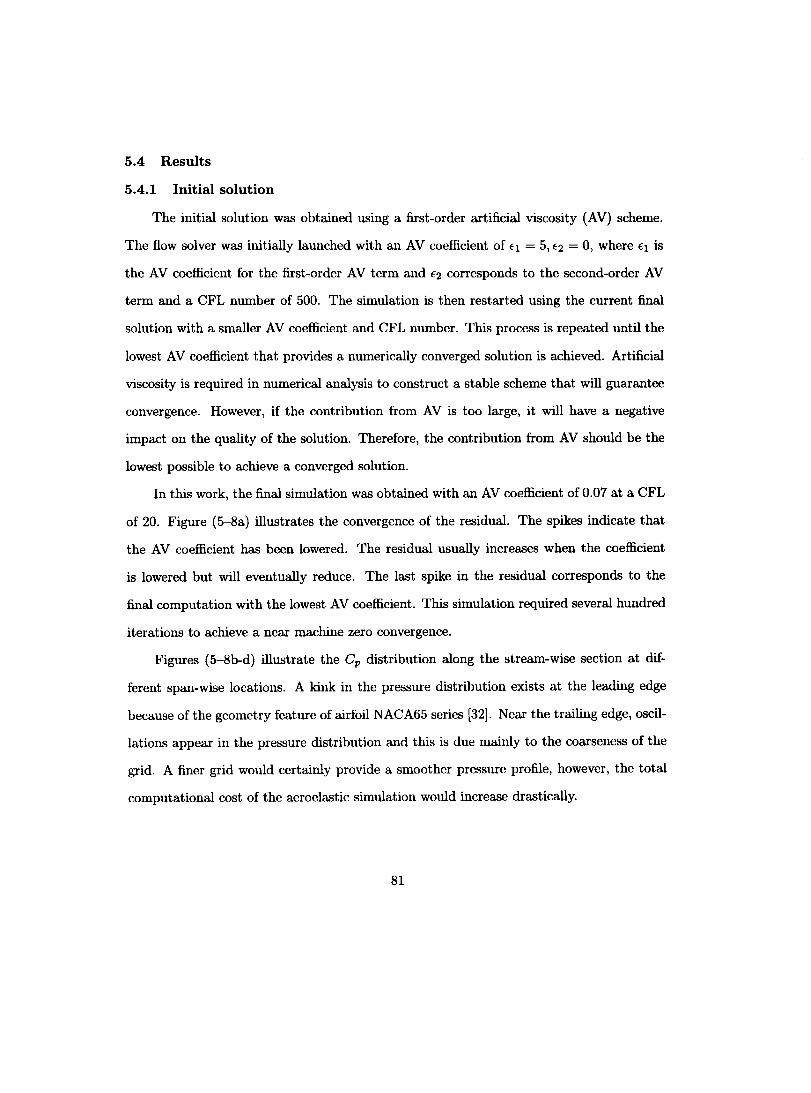
5.4 Results

5.4.1 Initial solution

The initial solution was obtained using a first-order artificial viscosity (AV) scheme.

The flow solver was initially launched with an AV coefficient of fI = 5, f2 = 0, where fI is

the AV coefficient for the first-order AV tenn and f2 corresponds to the second-order AV

term and a CFL number of 500. The simulation is then restarted using the current final

solution with a smaller AV coefficient and CFL number. This process is repeated until the

lowest AV coefficient that provides a numerically converged solution is achieved. Artificial

viscosity is required in numerical analysis to construct a stable scheme that will guarantee

convergence. However, if the contribution from AV is too large, it will have a negative

impact on the quality of the solution. Therefore, the contribution from AV should be the

lowest possible to achieve a converged solution.

In this work, the final simulation was obtained with an AV coefficient of 0.07 at a CFL

of 20. Figure (5-8a) illustrates the convergence of the residual. The spikes indicate that

the AV coefficient has been lowered. The residual usually increases when the coefficient

is lowered but will eventually reduce. The last spike in the residual corresponds to the

final computation with the lowest AV coefficient. This simulation required several hundred

iterations to achieve a near machine zero convergence.

Figures (5-8b-d) illustrate the Cp distribution along the stream-wise section at dif­

ferent span-wise locations. A kink in the pressure distribution exists at the leading edge

because of the geometry feature of airfoil NACA65 series [32]. Near the trailing edge, oscil­

lations appear in the pressure distribution and this is due mainly to the coarseness of the

grid. A finer grid would certainly provide a smoother pressure profile, however, the total

computational cast of the aeroelastic simulation would increase drastically.

81

,o~ r--~--~-~--~--~-----'

,o~

,o~

10.120:-----"'=-----;!,OO;;----::''''=----:200::;:---''''=------:!300 _.\op

(a) Residual History

o.,

-o.,

-0.3

-0.4

-o .•

(c) Cp distribution at z = 0.4

o.,

-o.,

-0.3

-0.4

-o .•

(b) Cp distribution at z = 0.2

o.,

-o.,

-0.2

-0.3

-0.4

-o .•

(d) Cp distribution at z = 0.6

Figure 5-8: Residual History and Cp distribution at different spanwise location for Flow around AGARD Wing 445.6 at Moo = 0.499

82

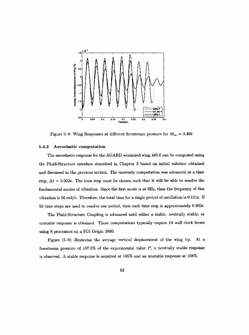
X 10-3

1.5r-'---r-----r-----,---..-----r------r----.------,

~ l 0.5

ë 1 0

i5. -0.5 i!! ~ -1 ~

f -1.5

< -2

~

0.15

fi fi.

(1

1\ 'f" f ,\ 'f V\J 1"

IV V \t

\1 l-l05%P pl --107.5%P --l08%P

0.2 0.25 0.3 0.35 0.4 Time(sec)

Figure 5-9: Wing Responses at difIerent freestream pressure for Mao = 0.499

5.4.2 Aeroelastic computation

The aeroelastic response for the AGARD weakened wing 445.6 can be computed using

the Fluid-Structure interface described in Chapter 3 based on initial solution obtained

and discussed in the previous section. The unsteady computation was advanced at a time

step, Ât = 0.002s. The time step must be chosen such that it will be able to resolve the

fundamental modes of vibration. Since the first mode is at 9Hz, then the frequency of this

vibration is 56 rad/s. Therefore, the total time for a single period of oscillation is 0.111s. If

50 time steps are used to resolve one period, then each time step is approximately 0.002s.

The Fluid-Structure Coupling is advanced until either a stable, neutrally stable, or

wlStable response is obtained. These computations typically require 14 wall dock hours

using 8 processors on a SGI Origin 3800.

Figure (5-9) illustrates the average vertical displacement of the wing tip. At a

freestream pressure of 107.5% of the experimental value P, a neutrally stable response

is observed. A stable response is acquired at 105% and an unstable response at 108%.

83

x ID·' 1.5r'-"'--,--,...-----.----,-----,,----.-----,

~ l 0.5

"ë

I~ ~ -1 ~

f -1.5

< -2

-2.5~-_=_=;__r-:':__~_7:_:_-_:'::_---::-'~===i::=:=..J o 0.05 0.1 0.15 0.2 0.25 0.3 0.35 TIIII8(NC)

Figure 5-10: Wing Responses with difIerent coupling instance for Moo 107.5%P

5.4.3 Effects of Coupling

0.499, Poo

As in the Isogai case, the number of coupling (or sub-iterations) per time step have an

efIect on the aeroelastic computation. Figure (5-10) illustrates that if a single sub-iteration

is performed the solution diverges. If a smaller time step is employed, then conceivably

a single sub-iteration would be sufficient. However, this would render the computation

intractable. Therefore, it is more desirable to use a larger time step with two sub-iterations

per time step.

5.4.4 Effect of Artificial Viscosity

As discussed earlier, a low AV coefficient is desirable. From figure (5-11), three aeroe­

lastic simulations are performed at various AV coefficients for the 107.5% freestream pres­

sure case. The reference computation is based on an AV coefficient of 0.07. At a higher

coefficient of 0.075, a stable response is obtained. A larger AV coefficient, indicates a larger

amount of numerical damping is present in the flow solver, thus a stable response would

84

x 10-' 2r.===~~~--~--~----~--~--1

::::::~::I 1.5 --8v:0.0151

Q. n F

A A ~ ~ ~ ~ 1 r ~ ~ :e "5

i 0.5

0

~ -0.5 ~

f -1 oC

-1.5 ~ ~ ~ ~ -1'1 ~ V \r ~ \

-2 0 0.05 0.1 0.15 0.2 0.25 0.3 0.35

Tirne(aac)

Figure 5-11: Wing Responses with different artificial viscosity for M 00

107.5%P 0.499, Poo

be observed for the same test case where a neutrally stable response was observed for a

smaller AV coefficient.

However, for the case, where the AV coefficient was 0.068, an unstable response was

attained. This indicates that a neutrally stable response would be observed at a lower

freestream pressure.

85

CHAPTER6 Conclusions

A modular fiuid-structure tightly coupled aeroelastic solver based on a 3D Euler or

Navier-Stokes solver, FENSAP, and structural solvers, in-house code for wing typical sec-

tion and finite element structural analysis package-MSCjNASTRAN-for wing, were de­

veloped to perform the fiutter simulation for a typical wing section and a wing. The first

aeroelastic solver predicted the fiutter boundary for subsonic and transonic fiow around a

typical wing section. The movement of shock waves on the wall boundary, the damping

and divergent self-excited oscillation were captured, and the transonic dip was observed.

For the 3D wing, the fiutter point at Mach number 0.499 and the damping and divergent

response were predicted. In both cases the results agree well with previous numerical or

experimental results.

The Modular approach for fiuid-structure interaction simulation provides the user the

flexibility to employ available structural or fluid solvers. The Fluid-Structure Interface

(FSI) developed in this work provides the ability to transfer loads and displacements be-

tween the fiuid and structural grids conservatively. The FSI is based on a node-to-element

mapping that allows the method to transfer loads and displacements from a 3D fiuid grid

to a low fidelity structural grid such as a fiat plate or even a beam.

Computation of accurate aeroelastic responses requires a detail analysis to the follow-

ing four aspects. First, the magnitude of the artificial viscosity term employed to stabilize

the numerical Euler equations must be low enough as not to affect the quality of the so-

lution. Results have shown that small changes to the artificial viscosity coefficient can

alter the aeroelastic response from neutrally stable to unstable. Secondly, to ensure proper

86

temporal resolution, time steps must be chosen such that the aeroelastic solution converges

to a periodic steady state solution as the time step is reduced.

Third, grid quality has a major impact on aeroelastic solutions. For the transonic test

case, the accurate capture of the shock wave, provides for better lift and most importantly

moment coefficients. Results have shown that grids with a higher resolution in the vicinity

of the shock wave provides more accurate pit ching angle and plunging displacement values.

For the AGARD test case at Mach 0.499, a mesh adaptation tool was used to improve

on the grid quality before aeroelastic simulation was performed. The accurate capture

of the leading edge peak pressure is of paramount importance to predicting the flutter

point. Accurate pressure distribution provides for an accurate representation of the moment

coefficient which has a large impact on aeroelastic cases.

Lastly, employing at least two sub-iterations per time step, allows for larger time steps

and thus a reduction in the total computational cost. The approach drastically reduces

lagging of either the fluid or structural solvers which is a common problem if OlÙy a single

iteratioll is perfonned per time step.

6.1 Future Work

The Fluid-Structure Interface presented in this work has established the framework

to couple various different fluid and structural solvers. The results presented in this work,

testifies to the versatility of the approach. Future work based on this framework can take

the following direction:

1. A natural next stage is the accurate prediction of aeroelastic response for three­

dimensional transonic viscous flows.

2. Apart from computing aeroelastic solutions, the future direction should involve the

design of an aircraft wing or rotorcraft blade to tailor the aeroelastic response. Wing

flutter and buffet reduces the lift cycle of the structure due to fatigue. Aeroelastic

87

design that minimizes fatigue will have a large impact on the total operating cost of

aircrafts.

88

References

[1] J. J. Alonso and A. Jameson. F\ùly-implicit time-marching aeroelastic solution. AIAA paper 94-0056, 32nd AIAA Aerospace Sciences Meeting and Exhibit, Reno, NV, Jan­uary 1994.

[2] K. Appa. Finite-surface. AIAA Journal, 26(5):495-496, 1989.

[3] G. S. Baruzzi, W. G. Habashi, J. G. Guevremont, and M. M. Hafez. A second or­der method for the finite element solution of the euler and navier-stokes equations. International Journal for Numerical Methods in Engineering, 20, 1995.

[4] J. T. Batina. Unsteady euler algorithm with unstructured dynamic mesh for complex­aircraft aeroelastic analysis. AIAA paper 89-1189, 1989.

[5] O. A. Bauchau and J. U. Ahmad. Advanced cfd and csd methods for multidisciplinary applications in rotorcraft problems. AIAA paper 96-4151, July 1996.

[6] O. O. Bendiksen. A new approach to computational aeroelasticity. AIAA paper 91-0939, APRIL 1991.

[7] R. M. Bennet, J. T. Batina, and H. Cunningham. Wing-flutter calculations with the cap-tsd unsteady transonic small-disturbance program. Jouranl of Aircraft, 26(9), 1989.

[8] S. A. Brown. Displacement extrapolation for cfd+csm aeroelastic analysis. AIAA paper 97-1090, 1997.

[9] P. C. Chen and L. R. Hill. A three-dimensional boundary elemen method for cfd/ csd grid interfacing. AIAA paper 99-1213, 1999.

[10] R. R. Craig. Structural Dynamics.

[11] S. S. Davis. Naca64aOlO (nasa ames model) oscillatory pitching. AGARD Report 702, 1982.

[12] E. H. Dowell(Editor), R. Clark, D. Cox, H. C. Curtiss Jr., J. W Edwards, K. C. Hall, D. A. Peter, R. Scanlan, E. Simiu, F. Sisto, and T. W. Strganac. A Modern Course in Aeroelasticity (Fourth Revised and Enlarged Edition). Kluwer Academic Publishers, Dordrecht, Netherlands, 2004.

89

90

[13] J. W. Edwards, R. M. Bennet, W. Whitlow Jr., and D. A. Seidel. Time-marching transonic flutter solutions including angle-of-attack effects. Jouranl of Airerajt, 20(11), 1983.

[14] R. E.Gordier and R. B. Melville. Transonic flutter simulations using an implicit aeroe­lastic solver pages. Jouranl of Airerajt, 37(5), 2000.

[15] L. E. Erikson. Generation of boundary-conforming grids around wing-body configu­ration using transfinite interpolation. AIAA Journal, 20(10):1313-1320, 1982.

[16] L.E. Eriksson. Generation of boundary-conformation grids around wing-body config­urations using transfinite interpolation. AIAA Journa~ 20(10):1313-1320, 1982.

[17] M. Farhangnia and G. P. Guruswamy. Transonic buffer associated aeroelasticity of a supecritical wing. AIAA paper 96-0286, 1996.

[18] C. Farhat, M. Lesoine, and N. Maman. Mixed explicitjimplicit time integration of coupled aeroelastic problem: Three-field formation, geometric conservation and distri­bution solution. International Journal for Numerical Methods in Engineering, 21:807-835, 1995.

[19] R. E. Gordnier and R. B. Melville. Transonic flutter simulation using an implicit aeroelastic solver. Jouranl of Airerajt, 37(5), 2000.

[20] G. P. Guruswamy. Unsteady aerodynamic and aeroelastic calculations for wings using euler equations. AIAA Journal, 28(3):461-469, 1990.

[21] G. P. Guruswamy. Vortical fiow computations on swept flexible wings using navier­stokes equations. AIAA Journal, 28(12):2077-2084, December 1990.

[22] G. P. Guruswamy. Coupled finite-differencejfinite-element approach for wing-body aeroelasticity. AIAA paper 92-4680, September 1992.

[23] G. P. Guruswamy. A review of numerical fiuidjstructures interface methods for com­putations using high-fidelity equations. Computers and Structures, 80:31-41, 2002.

[24] G. P. Guruswamyand C. Byun. Fluid-structural interactions using navier-stokes flow equations coupled with shell finite element structures. AIAA paper 93-3087, July 1993.

[25] G. P. Guruswamy and T.Y.Yang. Aeroelastic time-response analysis of thin airfoils by transonic code Itran2.

[26] R. L. Harder and R. N. Desmarais. Interpolation using surface curves. AIAA Journal, 9(2):189-191, 1972.

91

[27) D. G. Holmes and H. A. Chuang. 2d linearized harmonie euler flow analysis for flutter and forced response. Technieal report, Unsteady Aerodynamics, Aeroacoutics and Aeroelasticity of Turbomachines, and Propellers (6th Int. Symp.on), New York, 1993.

[28) K. Isogai. On the transonic-dip mechanism of flutter of a awept wing. AIAA Journal, 17(7):793-795, 1979.

[29) K. Isogai. Transonic dip mechanism of flutter of a awept wing:part ii. AIAA Journal, 19(9):1240-1242, 1981.

[30) K. A. Kousen. Nonlinear Phenomena in Computational Transonic Aeroelasticity. PhD thesis, Princeton University, Dept. of Mechanical and Aerospace Engineering, January 1989.

[31) H. G. Kussner. A comparison of methods used in flutter research. A GARD Report 592, Aug. 1972. Supplement, AGARD Manual of Aeroelasticity.

[32) C. Lepage. A Tight Two- Way Fluid-Structure Coupling for Aeroelastic Computations in the Time Domain. PhD thesis, Concordia University, Dept. of Mechanical and Industrial Engineering, July 2004.

[33) C. Y. Lepage and W. G. Habashi. Fluid-structure interactions using the ale formu­lation. AIAA paper 99-0660, 37th AIAA Aerospace Sciences Meeting and Exhibit, Reno, NV, Jan 1999.

[341 F. Liu, J. Cai, and y. Zhu. Calculation of wing flutter by a coupled fluid-structure method. Jouranl of Aircrajt, 38(2), 2001.

[35) S. Mittal and T. E. Tezduyar. A finite element study of incompressible flows past oscillating cylinder and airfoil. IJNMF 15-1073, 1992.

[36) M. Petyt. Introduction to Finite Element Vibration Aanalysis. Cambridge University Press, Cambridge, 1990.

[37) B. A. Robinson, J. T. Batina, and H. T. Y. Yang. Aeroelastic analysis of wing using the euler equation with a deforming mesh. Jouranl of Aircrajt, 28(11), 1991.

[38) D. M. Schuster, J. Vadyak, and E. Atta. Static aeroelastic analysis of fighter aircraft using a three-dimensional navier-stokes algorithm. Jouranl of Aircrajt, 27(9), 1990.

[39) J. M. Seigel, V. Parthasarathy, G. M. Kingsley, P. J. Dionne, V. J. Harrand, and J. J. LukerS. Application of a multi-disciplinary computing environment (mdice) for loosely coupled fluid-structural analysis,. AIAA paper 98-4865, 1998.

[40] G. Sitton. MSCjNastran Basic Dynamic Analysis User's Guide Vol 1. The MacNel­Schwendler Corporation, 1997.

92

[41] M. J. Smith. Acceration techniques for an aeroelastic euler method for a hovering rotor. Jouranl of Aireraft, 33(2), 1996.

[42] M. J. Smith. Evalution of computational algorithms suit able for fluid-structure inter­action. Jouranl of Aireraft, 37(2), 2000.

[43] M. J. Smith, D. H. Hodges, C. E. S. Cesnik, and K. J. Kenneth. An evaluation of computational algorithms to interface between cfd and csd methodologies. AIAA Paper 96-1400, AIAA/ ASME/ ASCE/ AHS/ ASC Structures, Structural Dynamics and Materials Conference and Exhibit,37th, Salt Lake City, UT, April 1996.

[44] C. V. SPain. Development of nastran finite element and aeroelastic models of agard standard configuration i - wing 445.6. InternaI Report, Lockheed Martin Engineering and Sciences, 2000(draft).

[45] J. L. Steger. Calculation of transonie aileron buzz. AIAA Journal, 18(3):249-255, 1980.

[46] J. T.Batina. Unsteady transonie algrithm improvements for realistic aircraft applica­tion. AIAA paper 88-0105, Jan. 1988.

[471 P. D. Thomas and C. K. Lombard. Geometrie conservation law and its application to flow computation on moving grids. AIAA Journal, 17(10):1030-1037, Oct. 1979.

[481 G. Tzong, H. H. Chen, K. C. Chang, T. Wu, and T. Cebeci. A general method for calculating aero-structure interaction on aircraft configurations. AIAA paper 96-3982, 1996.

[49] K. Willcox and J. Peraire. Aeroelastic computations in the time domain using unstruc­tured meshes. International Journal for Numerical Methods in Engineering, 40:2413-2431, 1997.

[50] A. Wong, H. Tsai, J. Cai, Y. Zhu, and F. Liu. Unsteady flow calculation with a multibolck moving mesh algorithm. AIAA paper 2000-1002,2000.

[51] E. C. Jr. Yates, N. S. Land, and Foughner J. T. Jr. Measured and calculate subsonic and transonic flutter characteristics of a 45 sweptback wing plantform in air and in freon-12 in the langley transonic dynamics tunnel. AGARD Report TN D-1616, 1963.