FLUID MECHANICS AND MATHEMATICAL STRUCTURES

PHILIP BOYLANDDepartment of MathematicsUniversity of FloridaGainesville, FL 32611-8105, USA

E-mail: boyland@math.ufl.edu

To Ed Spiegel on his 70th birthday.

Abstract. This paper provides an informal survey of the various mathe-matical structures that appear in the most basic models of fluid motion.

1. Introduction

Fluid mechanics is the source of many of the ideas and concepts that arecentral to modern Mathematics. The vestiges of these origins remain inthe names of mathematical structures: flows, currents, circulation, frames,. . ., and in the names of the distinguished mathematician-scientists whichpervade the terminology of both fields: Euler, Bernoulli, Stokes, Cauchy,Lagrange, . . .. Mathematicians have abstracted and vastly generalized ba-sic fluid mechanical concepts and have created a deep and powerful bodyof knowledge that is unfortunately now mostly inaccessible to fluid me-chanicians, while mathematicians themselves have lost all but a passingknowledge of the physical origins of many of their basic notions.

This paper provides an informal survey of the various mathematicalstructures that appear in the most basic models of fluid motion. As befitsthis volume it is strictly pedagogical. There are no original results, and mostof what we say here has been known for at least a century in one guise oranother. In style it attempts to reproduce the informal tutorials that tookplace during the Newton Institute program in Fall, 2000. Mathematicalobjects are described informally with an emphasis on their meaning inFluid Mechanics. Many formulas are stated without proof. The paper ismeant to be a friendly introduction to basic concepts and ideas and will

2

hopefully provide an intuitive foundation for a more careful study of theliterature. Readers are strongly encouraged to consult the references givenin each section.

In describing the fluid model we give primacy to the actual evolutionof the fluid, to the fluid flow, as opposed to the velocity fields. This agreeswith our direct experience of seeing fluids move as well as being very naturalin the mathematical progression we describe. While conceptually valuable,this point of view is computationally very impractical. The basic equationsof Fluid Mechanics are framed in terms of the velocity fields. Solutions ofthe equations are difficult to obtain, but formulas for the fluid motions arevirtually nonexistent.

One of the goals of the paper is to introduce students of fluid mechanicsto the “world view” of modern Mathematics. A common view among math-ematicians is that Mathematics is the study of sets with structures and ofthe transformations between them. From this point of view, the basic modelof Fluid Mechanics is the set consisting of the fluid body and the variousadditional structures that allow one to discuss such properties as continu-ity, volume, velocity and deformation. The flow itself is a transformationof the fluid body to itself and a basic object of study is the transport ofstructures under the flow.

It is considered a mathematical virtue to use just those structures whichare needed in a given situation and no more. The goal is not to be mind-lessly abstract but rather to discover and illustrate what is essential andfundamental to the task at hand. This has the added advantage that con-clusions have the widest applicability. Thus we develop the fluid model stepby step, introducing structures to fit certain needs in the modelling process.When possible coordinate free terminology and notation is used. We invokethe usual argument in its favor: anything fundamental shouldn’t dependon the choice of coordinates and being forced to treat computational ob-jects as global entities provides a new and sometimes valuable perspectiveon familiar operations. We do, however, try to connect new objects withfamiliar formula, and we try to be clear when formulas are only valid inusual Euclidean space.

We have attempted to keep the paper accessible to a wide audience, butsome fluid mechanical terminology is used without explanation. Generalreaders may consult any standard text; the mathematically inclined mayprefer [22], [7], [16] or [5].

2. Basic Kinematics and Mathematical Structures

We begin by describing the most fundamental mathematical structures usedin modelling the simplest type of fluid behavior. Unless otherwise stated the

3

fluid is three-dimensional; two-dimensional flow can be treated similarly.

2.1. THE FLUID REGION, FLUID MAPS AND CARDINALITY

The first step is to model the fluid region itself. In Fluid Mechanics it isusually said that the fluid is a continuum. In mathematical language thissays that, at least locally, the fluid looks like usual two or three-dimensionalspace. We allow the possibility that on large scales the fluid is not flat, butrather can curve back on itself like the surface of the (almost) sphericalearth. Objects with a local structure like the plane or three space, butperhaps nontrivial global behavior are called 2- or 3-dimensional manifolds.A fluid particle is a mathematical point in the manifold. The generic fluidregion or fluid body is denoted B.

The modelling of the fluid as a manifold has many implications andsome obvious problems. It is clearly false on very small scales as it com-pletely ignores the molecular nature of fluids. In addition, a mathematicalpoint obviously has no physical meaning. Nonetheless, the theories andtechnologies based on continuum models have been wildly successful andwe can proceed with confidence using a manifold model.

As a fluid flows particles are transported. In terms of the model the fluidmotion is defined as the collective motion of the particles. It is assumedthat the individual particles do not split into pieces, and each has a welldefined future and remains distinguished for all times. This means that theevolution is described by the transformation that takes the initial positionof a particle as input and gives the position after a time T as the output.Thus for each time T the evolution of the fluid after time T is describedby a function (or map), f , from the initial region occupied by the fluid,B0, to the region occupied after time T , BT . The usual notation for this isf : B0 → BT , indicating that f is a function with domain B0 and range BT .The function f is called the time-T fluid map. The typical point in a fluidregion is labelled p, q, etc. Note that these label the geometric position inthe region and not the fluid particles, and so they do not move with theflow.

During their evolution it is further assumed that fluid particles do notoverlap, coalesce or collide. Thus if two points are distinct, then their po-sitions after time T are different, or p 6= q implies f(p) 6= f(q), and so fis a one-to-one (or injective) function. Since by definition, BT is the fluidregion after time T , we have that f : B0 → BT is an onto (or surjective)function, which is just to say that for any p in BT there is a p in B0 withf(p) = p, i.e. the particle at p came from somewhere.

Summarizing, the most basic assumptions on a fluid map is that it isone to one and onto, i.e. it is a bijection, or what is sometimes termed a

4

one-to-one correspondence. This means that f preserves the “number” offluid points. This idea is formalized as the most fundamental property of aset, its cardinality. By definition, two sets have the same cardinality exactlywhen there is a one-to-one correspondence between them. While this maynot seem like much information about the fluid map it is worth noting thatthere are sets with different cardinality.

Exercise 2.1 Show that there is a one-to-one correspondence between theset of points in the interval, 0 ≤ x ≤ 1, and the set of points in the unitsquare in the plane, 0 ≤ x ≤ 1, 0 ≤ y ≤ 1, but that these sets have adifferent cardinality from the set of integers 0,±1,±2, . . ..

A bijection f always has an inverse map, usually denoted f−1, whichby definition satisfies f f−1 = f−1 f = id. While the inverse of a fluidmap always exists, there is no assumption in general that it is a physicallyreasonable fluid map, though in certain cases it can be.

Elementary set theory is covered in the first sections of most textbooksin Algebra or Topology, [13] is a standard text, and [26] is recreational butinformative.

2.2. STRUCTURES, TRANSPORT, AND CATEGORIES

At this point our fluid is described by the most basic of mathematicalobjects, sets and a transformation. We pause now to introduce some generalnotions about mathematical structures and how they are transported bytransformations.

Mathematical structures take many forms. The most basic examplesare an order structure which declares which elements are larger than others,a topology which is a distinguished collection of subsets, and an algebraicstructure which is a binary operation on the set which satisfies certainrules. Other common structures are made out of various kinds of functionsinto or out of the set. For example, a velocity field is a map out of theset, it assigns a vector to each point in the set. A loop is a map from thecircle into a set. The collection of all tangent vectors to a space are turnedinto the tangent bundle, which in turn is the basis for other structures liketensors, Riemannian metrics and differential forms. The general intuitionis that a structure is something that “lives on top of ” the set, representingadditional information and properties.

If a transformation between underlying sets is sufficiently well behavedit induces a map on the various structures, transforming a structure onone set to the same kind of structure on the other set. For example, inideal magnetohydrodynamics the fluid flow transports the magnetic vectorfield at time zero to the magnetic vector field after a time T . The generalmathematical rubric is that transport in the direction of the map is called

5

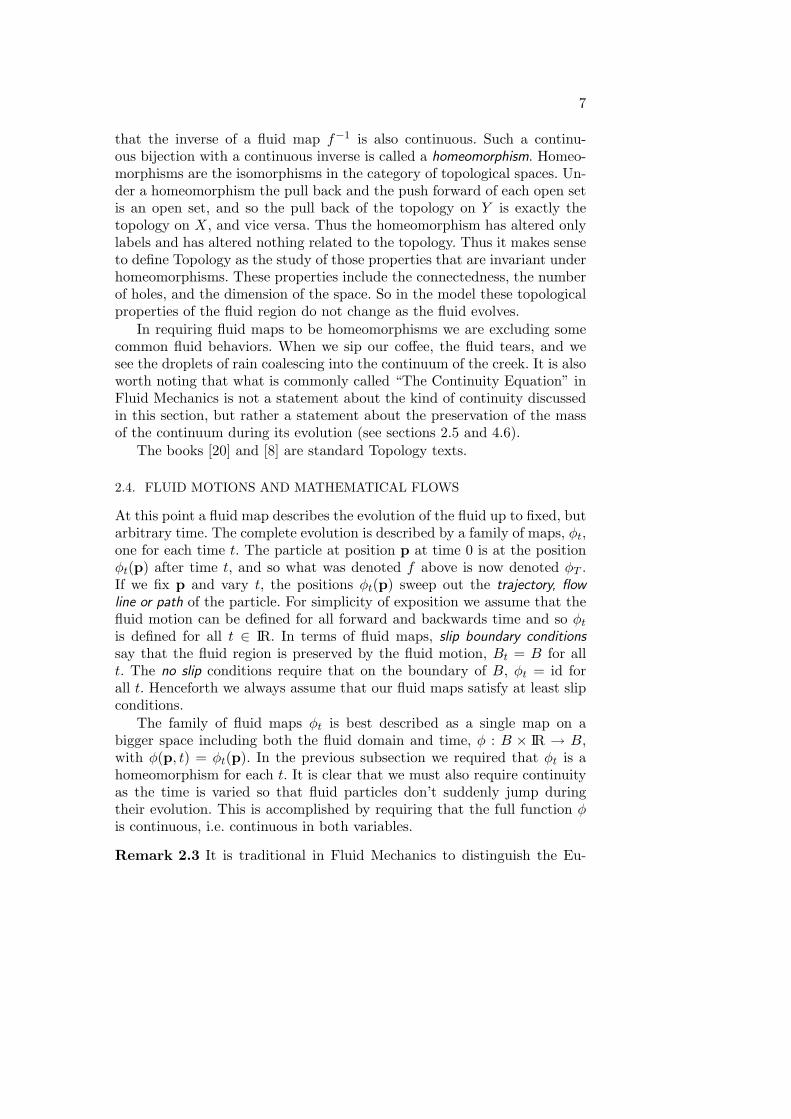
push forward while pull back is an induced map that goes in the directionopposite to the given map. If the map we are studying is a fluid map, thenthe push forward transports the structure in forward time while pull backrefers to transport from the future backward, usually back to the initialstate of the system. The standard notation puts a star on the given map toindicate the induced map on structures, with a subscript indicating a pushforward and a superscript indicating a pull back. Thus if f is a fluid mapand α is a structure (say a magnetic field) then f∗(α) is this vector fieldpushed forward by the fluid evolution and f∗(α) indicates its pull back.

Since a fluid map f is invertible, pulling back is the same as pushingforward by the inverse f−1, and we will freely pass between the two. De-pending on the structures it is usually most natural to either pull back orelse push forward. As a general guideline when a structure is defined by amap into the set it is pushed forward. For example, a loop in the fluid regionis a map Γ : S1 → B0, and this naturally pushes forward to the same kindof structure on BT since the composition f Γ is a map S1 → BT calledf∗Γ. On the other hand, a structure defined by maps out of the set, say ascalar field α on BT , is most naturally pulled back because α f = f∗α isa map out of B0. Another basic pull back is that of a set. If N is a sub-set of the fluid region BT , then its pull back is a subset of B0 defined byf∗(N) = p in B0 : f(p) is in BT ; this set is also often denoted f−1(N).

The notion of a mathematical category and its morphisms formalizesmany of the notions of sets, structures and transformations. The most ba-sic category is the collection of sets and other categories consist of sets withsome specific additional structure such as topological spaces, vector spaces,smooth manifolds, or flows on manifolds. The morphisms associated witha category are the maps between sets that preserve the structure, i.e. theinduced map on structures is defined and a transported structure is com-patible with the pre-existing one. For example, linear transformation arethe morphisms of vector spaces and continuous functions are the morphismsof topological spaces.

An isomorphism in a category is a morphism that is a bijection and itsinverse is also a morphism. Most of the commonly studied categories havetheir own traditional name for their isomorphism such as bijection in thecategory of sets, homeomorphism in the category of topological spaces, andisometry in the case of geometries. Within a given category isomorphic ob-jects are considered indistinguishable, and indeed a rather formal definitionof a mathematical area of study is that it studies those properties that arepreserved by the morphisms in its particular category.

The text [15] is a standard reference.

6

2.3. CONTINUITY AND TOPOLOGY

Exercise 2.1 clearly indicates that a bijection can scramble a fluid domainvery badly, prompting the requirement that fluid motions preserve the con-tinuum nature of the fluid, not tearing or distorting it too wildly. Thisrequirement is the essence of Topology and its morphisms, the continuousfunctions, and is expressed in the assumption that fluid particles which aresufficiently close initially should still be close after evolving for time T . Thetechnicalities arise from defining “sufficiently close” and “still be close”.

A topology as a structure on a set is simply a collection of distinguishedsubsets called the open sets (there are conditions which are not importanthere). Open sets are the allowable neighborhoods of the point and neigh-borhood is used synonymously with open set. A property is true for pointssufficiently close to p if it is true for all open sets containing p. In the cate-gory of sets with topologies (topological spaces) the morphisms or structurepreserving maps are the continuous functions. A function g : X → Y be-tween two topological spaces is called continuous if the pull back of an openset is open. Thus for each open set U in Y it is required that f∗(U) is anopen set in X, or by acting on all open sets, it is required that the pullback of the topology on Y is compatible with the topology on X.

Sequences provide a simple way to connect this abstraction with themore physical condition that nearby fluid particles should stay near eachother. In terms of a given topology, the sequence (pn) converges to thepoint p0, written pn → p0, when any neighborhood V that contains p alsocontains the tail of the sequence, i.e. there is an N so that n > N impliesthat pn ∈ V . If f is the time T fluid map, the flow preserving the continuumstructure clearly requires that pn → p0 implies f(pn) → f(p0). This saysthat any neighborhood U of f(p0) must contain the tail of the sequencef(pn). But transporting this data back to the fluid at time zero we seethat the convergence after time T requires that pn ∈ f∗(U) for n > N .But since pn → p0, this would be achieved by requiring that f∗(U) is itselfa neighborhood, which is the case if f is continuous in the sense definedabove.

Exercise 2.2 In the standard topology on IRn a set U is open when forevery p ∈ U there is an r, so that the ball Br(p) = q : |q − p| < ris wholly contained in the set U . Show that in this case the definition ofcontinuity of a function using the pull back of open sets is the same as theusual one: f is continuous at p if for all ε there exists a δ so that

|q− p| < δ implies |f(q)− f(p)| < ε .

In the fluid model particles which are sufficiently close after time Tshould come from particles which were close at time zero. Thus we assume

7

that the inverse of a fluid map f−1 is also continuous. Such a continu-ous bijection with a continuous inverse is called a homeomorphism. Homeo-morphisms are the isomorphisms in the category of topological spaces. Un-der a homeomorphism the pull back and the push forward of each open setis an open set, and so the pull back of the topology on Y is exactly thetopology on X, and vice versa. Thus the homeomorphism has altered onlylabels and has altered nothing related to the topology. Thus it makes senseto define Topology as the study of those properties that are invariant underhomeomorphisms. These properties include the connectedness, the numberof holes, and the dimension of the space. So in the model these topologicalproperties of the fluid region do not change as the fluid evolves.

In requiring fluid maps to be homeomorphisms we are excluding somecommon fluid behaviors. When we sip our coffee, the fluid tears, and wesee the droplets of rain coalescing into the continuum of the creek. It is alsoworth noting that what is commonly called “The Continuity Equation” inFluid Mechanics is not a statement about the kind of continuity discussedin this section, but rather a statement about the preservation of the massof the continuum during its evolution (see sections 2.5 and 4.6).

The books [20] and [8] are standard Topology texts.

2.4. FLUID MOTIONS AND MATHEMATICAL FLOWS

At this point a fluid map describes the evolution of the fluid up to fixed, butarbitrary time. The complete evolution is described by a family of maps, φt,one for each time t. The particle at position p at time 0 is at the positionφt(p) after time t, and so what was denoted f above is now denoted φT .If we fix p and vary t, the positions φt(p) sweep out the trajectory, flowline or path of the particle. For simplicity of exposition we assume that thefluid motion can be defined for all forward and backwards time and so φtis defined for all t ∈ IR. In terms of fluid maps, slip boundary conditionssay that the fluid region is preserved by the fluid motion, Bt = B for allt. The no slip conditions require that on the boundary of B, φt = id forall t. Henceforth we always assume that our fluid maps satisfy at least slipconditions.

The family of fluid maps φt is best described as a single map on abigger space including both the fluid domain and time, φ : B × IR → B,with φ(p, t) = φt(p). In the previous subsection we required that φt is ahomeomorphism for each t. It is clear that we must also require continuityas the time is varied so that fluid particles don’t suddenly jump duringtheir evolution. This is accomplished by requiring that the full function φis continuous, i.e. continuous in both variables.

Remark 2.3 It is traditional in Fluid Mechanics to distinguish the Eu-

8

lerian and the Lagrangian perspective. In the first, the labels are pinneddown in the fluid region, in mathematical language they are local coordi-nates in the manifold modelling the fluid. In the Lagrangian perspective,the fluid particle is labelled and that label remains on the particle as itmoves. In addition, the Eulerian perspective is a field theory, focusing onthe velocity vector field while the Lagrangian focuses on the motions orflow lines of particles. The point of view here is mixed: we always labelusing a fixed, pinned down coordinate system in the fluid region and neveruse Lagrangian or advected coordinates, but the primary focus is on themotion of particles. It is also traditional in Fluid Mechanics to use x for theEulerian coordinate, and to denote a trajectory as x(t), indicating how thecoordinate varies as a function of time. This use of the same symbol to indi-cate both a coordinate and a function of time makes many mathematiciansuncomfortable; it represents an unacceptable confusion of different classesof mathematical objects. Thus we denote the time evolution by a distinctfunction, φ, which encapsulates all the time and space evolution. To avoidconfusion with the training of fluid mechanicians, while maintaining thenotation x = (x1, x2, x3) for the local coordinates, p and q are used here todenote the typical point in the fluid region (labelled by the fixed coordinatesystem) rather than the more common mathematical x or x.

There is a useful distinction among fluid motions based on how thefuture of particles depends on the starting time. Pick a fixed, but arbitrarylocation in the fluid region and monitor the future of the particle that isthere at time 0 and also that of the particle that is there at some latertime. If these futures are always the same the flow is steady, otherwise it isunsteady.

This distinction has a nice formulation in terms of the algebra of thetime parameter, i.e. of the real line. Begin the evolution of the fluid particleat p and flow for time t, now at this point begin again and flow for time s,so we are at the point φs(φt(p)). On the other hand, we could start at p,flow for time t and then continue without restarting time for another timeinterval s, ending up at the point φs+t(p). The flow is steady exactly whenthese points are the same for all s, t and points p, or in terms of the fluidmaps, φs φt = φs+t. This group law coupled with the fact that φ0 is theidentity map says that a steady flow is an action of the real numbers on theregion B. This implies, in particular, that the inverse maps be computedby reversing time, φ−1

t = φ−tWithin most of mathematics the word flow refers to this kind of action of

the reals on a space. In particular, mathematical flows always correspond tosteady fluid flows. For this reason the general, perhaps unsteady, evolutionof a fluid is called here a fluid motion reserving the word flow for steadyflows.

9

Two simple examples of one-dimensional flows are the linear flow, φt(p) =p + rt, and the exponential flow, φt(p) = pert, where r is a real number.In these cases the group law of the action corresponds to the standard dis-tributive and exponential laws, respectively. Flows correspond to solutionsof time-independent differential equations, and it is remarkable that anysuch solution yields a flow with nice algebraic properties.

The simplest unsteady fluid motions are periodic. A fluid motion (orfluid map φt) is called periodic if starting at an initial time t at the point pyields the same future as starting at the same point at a time P later, whereP is called the period. This implies that φt+P = φt φP , and letting t =(n−1)P for an integer n, that φnP = φP φP . . . φP (n times). Thus if wedefine the Poincare map as g = φP , its iterates (repeated self compositions)satisfy gn = φnP , and so they describe the evolution of the fluid. ThePoincare map is often called the stroboscope map, as it corresponds toviewing the fluid under a light that turns on once each period.

If we have a fluid motion φt on a region B and a homeomorphism hfrom B to another region B, we can push forward the flow to one on B bythe rule h∗(φt) = h φt h−1. The motion for time T on B is obtained byfirst coming back to B via h−1, then flowing from that point via φT , andthen going back to B via h. If the homeomorphism is from B to itself, itrepresents a change of coordinates, and if h∗φt = ψt one says that two flowsφt and ψt are the same fluid motion up to change of coordinates by h.

2.5. INCOMPRESSIBILITY, MASS CONSERVATION AND MEASURES

If there are no mechanisms for inflow or outflow as a fluid subregion evolvesits mass stays the same. Similarly, if there are no mechanisms to compress orexpand regions of the fluid, then the volume of fluid subregions is preservedunder the evolution. Both of these properties can be included in the modelby postulating measures that are invariant under the fluid motion.

A measure is a rule which assigns a non-negative number to varioussubsets of the main set (again, there are additional technicalities that arenot crucial here). In a fluid model, the measure of a subset could representthe mass of the fluid in the subset, or perhaps the volume of the subset.Thus if m(U) is the mass of the fluid contained in the region U , thenmass conservation of the flow φt is expressed by m(φt(U)) = m(U) for allmeasurable sets U and all times t. Similarly, if ν(U) is the usual three-dimensional volume (Lebesgue measure) of a set U in IR3, then a fluid flowis incompressible if ν(φt(U)) = ν(U) for all measurable sets U and all timest.

Measures are most commonly used for integration, and one writes∫U α dν

for the usual integral of the real valued function α over the region U , and

10

thus ν(U) =∫U dν. A density ρ is a real-valued function which represents

the “measure per unit volume”, or more precisely, ρ is a density for themeasure m, exactly when m(U) =

∫U ρ dν. One then writes dm = ρ dν.

If g : X → Y is a function, we can use it to transport measures. Given ameasure m on X, its push forward to Y is g∗m. It is defined by the rule thatthe measure g∗m assigns to a subset V of Y is the measure of g∗(V ), or insymbols, g∗m(V ) = m(g∗(V )). Thus a fluid motion φt preserves the massgiven by the measure m exactly when φt∗m = m, for all t (in the unsteadycase m may be time dependent). Similarly, incompressibility is expressedby φt∗ν = ν, for all t.

¿From a strictly kinematic point of view there is little difference betweenpreserving a mass m or preserving the volume ν. This is consequence of atheorem of Oxtoby and Ulam [21] (Moser [19] in the smooth category). Ifthe mass density ρ is a reasonable function and for simplicity we assumethat the total mass equals the total volume,

∫ρ dν =

∫dν, then the

theorems give a homeomorphism (diffeomorphism) h of B to itself whichpushes forward m to ν, h∗m = ν. Thus if φt preserves m then by changingcoordinates by h, the fluid motion h∗(φt) preserves ν.

Elementary measure theory and integration is covered in most textbooksin Analysis, [12] is a measure theory standard.

2.6. DIFFERENTIABILITY

The laws of mechanics are expressed using derivatives, and indeed, thedevelopment of mechanics went hand in hand with the invention of calculus.The continuity of the fluid motion arose from the need to preserve thecontinuum structure of the fluid body. But the assumption that the fluidregion is locally Euclidean gives more than just a local topology, thereis also the algebraic structure of Euclidean space as a vector space. Theassumption of differentiability of fluid motion means that on small enoughscales the fluid map looks like a linear map of a vector space to itself. Thisis made precise by Taylor’s theorem and its converse which says that a mapf is differentiable exactly when it is linear up to an error of specified type.More precisely, in Euclidean space the matrix A is the first derivative ofthe map f at the point p exactly when

f(p + h) = f(p) +Ah + o(|h|) , (1)

with |h| the usual Euclidean norm and o(|h|) representing a quantity r(h)that goes to zero sufficiently fast so that r(h)

|h| → 0 as h→ 0.The matrix A is, of course, the usual Jacobian matrix, for which there

are numerous notations; its (i, j)-th entry is ∂fi/∂xj . When f is real valued,i.e. has only one component, then the derivative matrix is a row vector

11

representing the gradient, ∇f . It is common in Fluid Mechanics to also use∇ in the multidimensional case, and so we shall denote the full derivativeas ∇f , or ∇f(p). A function f is continuously differentiable if a matrix Asatisfying (1) exists at each point p and the matrices vary continuouslywith the evaluation point. In this case one writes f ∈ C1.

Higher derivatives can be defined using the analog of (1). A functionis C2 when it locally looks like a quadratic polynomial up to an error ofo(|h|2). The notation for the analog of (1) grows complicated, but in thesimplest case of a real valued function α, C2 means that

α(p + h) = α(p) +∇α · h + hT ·H(α) · h + o(|h|2) ,

where H(α) is the Hessian matrix of α, ( ∂2α∂xi∂xj

), and the Hessian must vary

continuously with the evaluation point. Continuing, a function is Ck if itlocally looks like a degree k polynomial up to order o(|h|k). If a functionis Ck for all k, it is called C∞. A condition that is even stronger than C∞

is the requirement that the Taylor’s series converges in a neighborhood ofeach point. Such functions are called real analytic and their class is denotedCω.

Exercise 2.4 Let the real valued function α be defined by α(0) = 0 andfor x 6= 0, α(x) = exp(−1/x2). Show that all orders of derivatives at 0 areequal to 0 and thus the Taylor’s series about 0 is identically zero. However,the function α is not identically zero in any neighborhood of the origin, andso α is an example of a C∞ function that is not Cω.

On a manifold, a function is Ck if it is Ck in local coordinates in thedomain and the range, and we need to treat the derivative as a linear trans-formation rather than a matrix. The matrix represents the linear transfor-mation in particular coordinates, but it is the linear transformation thathas coordinate free meaning.

In formulating differentiability from the structural point of view, theobjects in the category are C∞-manifolds. These are manifolds in whichC∞-compatible local coordinates can be defined. The morphisms are C∞-maps, and the isomorphisms are called diffeomorphisms, A diffeomorphismis a C∞-bijection whose inverse is also C∞. This category is the subject ofDifferential Topology. Henceforth we assume that fluid maps φt are C∞-diffeomorphisms for each t, and further, that the family itself is C∞ in t.It is worth noting that C3 is enough differentiability to do virtually all ofFluid Mechanics, but we shall not deal with that level of technicalities here.

Introductions to Differential Topology are given in [17] and [24], and[11], [6], and [14] are standard texts.

12

3. Vector Fields and the Tangent Bundle

At this point we have developed all the basic kinematic assumptions for thesimplest models of fluid flow. Forces enter into the models by their actionon velocity fields, the prototypical example of a vector field. Vector fields asa mathematical structure are the basis of many additional structures andoperations, and in this section we discuss some of those that are valuable indescribing fluid motions. Principal among these are the tangent bundle andother structural bundles that live “above” the fluid body. The fluid motionand its derivatives induce an action on these bundles that transport thevarious structures. The nature of this transport is the key to describinggeometric and topological aspects of the fluid motion.

3.1. VECTOR FIELDS AND THE VELOCITY FIELD

Given a fluid motion φt, its velocity field u at the point p at a time t is theinstantaneous velocity of the fluid particle that occupies that point at thattime. Note that this is the particle that started at φ−t(p) at time zero, andso

u(p, t) =∂φ

∂t(φ−t(p), t) ,

oru(φt(p), t) =

∂φ

∂t(p, t) . (2)

This is sometimes called the advection equation. Given a velocity field u,its fluid motion φt is obtained by solving the differential equation given by(2). It is easy to check that a fluid motion is steady as defined in Section2.4 if and only if its velocity field is time independent, u(p, t) = u(p),and the motion is T -periodic exactly when the velocity field is T -periodic,u(p, t+ T ) = u(p, t).

Exercise 3.1 The planar velocity field u(p) = (−p2, p1) represents uni-form counter-clockwise fluid motion. Show that its flow is φt(p1, p2) =(p1 cos(t) − p2 sin(t), p1 sin(t) + p2 cos(t)), and that in this case the groupproperty φtφs = φs+t is a reflection of standard trigonometric identities.

The velocity field at a fixed time is an example of a vector field, i.e. arule that assigns a vector to each point in the fluid region. Other commonexamples of vector fields are the magnetic field and the vorticity field. Wewill adopt the fairly standard mathematical convention that the terminol-ogy “vector field” refers to a time independent field. Through equation (2)mathematical flows and vector fields go hand in hand and it is usual topass freely from one to the other without comment.

In certain circumstances the time parameterization of a flow is not im-portant, and one wants to think of the trajectories as just curved lines in

13

space. In this case it is common in the sciences to call the curve constitut-ing the trajectory a field line, as in a magnetic field line and a vortex (field)line. The mathematical name for a way to fill a manifold with a collectionof curves is a one-dimensional foliation, and the individual curves are calledthe leaves. Note that the nonzero scalar multiple of a given nonvanishingvector field, αu, gives the same foliation as the original field, but gives riseto a different flow.

3.2. THE TANGENT BUNDLE

There is a common and quite understandable confusion that occurs earlyin a student’s mathematical training; is the base of a vector at the origin orat the point along a curve to which it is tangent? This usually leads to themathematical vector space called IR3 being somehow conceptually distinctin the student’s mind from the physical notion of velocity vectors.

The resolution of this unsatisfactory state is to attach a copy of thevector space IR3 to each point of three-dimensional space and then one canaccommodate all possible vectors being based at all possible points. Theresulting object is the tangent bundle of three space, and is denoted T IR3.It is equal to IR3 × IR3, with the first factor holding base points and thesecond the tangent vectors. The collection of vectors attached to a singlebasepoint p is called the tangent space or fiber at that point and is writtenTpIR3.

A vector field assigns a vector to each basepoint in IR3. Thus properlyspeaking a vector field is a map U : IR3 → T IR3. Amongst all such mapsvector fields have the distinguishing property that they map a basepoint toa vector based at that point. This is symbolically expressed by defining theprojection π : T IR3 → IR3 which takes a vector to its basepoint π(p, ~v) = p.A vector field then satisfies π U = id. Since it picks out just one vector“above” each point, a vector field is called a cross section of the tangentbundle.

The velocity field studied in Exercise 3.1 is formally written as U(p1, p2) =(p1, p2,−p2, p1). It is clear why in practise the first two components are usu-ally suppressed, but it is equally clear that they need to be there in theproper understanding of a vector field. A compromise is to use the basepoint as a subscript, and so, for example, vp represents a vector based atp.

For a fluid region B contained in IR3, its tangent bundle is denotedTB and is also a Cartesian product TB = B × IR3. For a 3-dimensionalmanifold the collection of tangent vectors based at a single point is alwaysthe vector space IR3, and locally any tangent bundle looks like a product,but in general the entire bundle is not a product. The simplest example

14

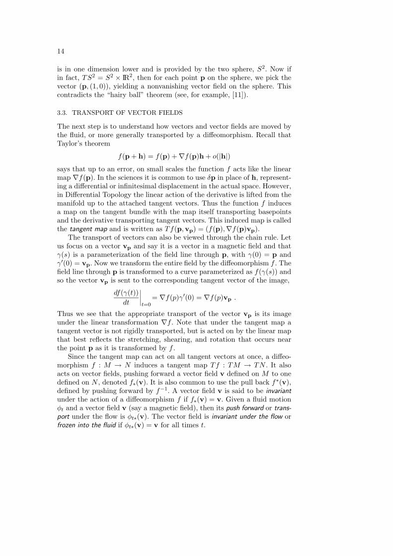
is in one dimension lower and is provided by the two sphere, S2. Now ifin fact, TS2 = S2 × IR2, then for each point p on the sphere, we pick thevector (p, (1, 0)), yielding a nonvanishing vector field on the sphere. Thiscontradicts the “hairy ball” theorem (see, for example, [11]).

3.3. TRANSPORT OF VECTOR FIELDS

The next step is to understand how vectors and vector fields are moved bythe fluid, or more generally transported by a diffeomorphism. Recall thatTaylor’s theorem

f(p + h) = f(p) +∇f(p)h + o(|h|)

says that up to an error, on small scales the function f acts like the linearmap ∇f(p). In the sciences it is common to use δp in place of h, represent-ing a differential or infinitesimal displacement in the actual space. However,in Differential Topology the linear action of the derivative is lifted from themanifold up to the attached tangent vectors. Thus the function f inducesa map on the tangent bundle with the map itself transporting basepointsand the derivative transporting tangent vectors. This induced map is calledthe tangent map and is written as Tf(p,vp) = (f(p),∇f(p)vp).

The transport of vectors can also be viewed through the chain rule. Letus focus on a vector vp and say it is a vector in a magnetic field and thatγ(s) is a parameterization of the field line through p, with γ(0) = p andγ′(0) = vp. Now we transform the entire field by the diffeomorphism f . Thefield line through p is transformed to a curve parameterized as f(γ(s)) andso the vector vp is sent to the corresponding tangent vector of the image,

df(γ(t))dt

∣∣∣∣t=0

= ∇f(p)γ′(0) = ∇f(p)vp .

Thus we see that the appropriate transport of the vector vp is its imageunder the linear transformation ∇f . Note that under the tangent map atangent vector is not rigidly transported, but is acted on by the linear mapthat best reflects the stretching, shearing, and rotation that occurs nearthe point p as it is transformed by f .

Since the tangent map can act on all tangent vectors at once, a diffeo-morphism f : M → N induces a tangent map Tf : TM → TN . It alsoacts on vector fields, pushing forward a vector field v defined on M to onedefined on N , denoted f∗(v). It is also common to use the pull back f∗(v),defined by pushing forward by f−1. A vector field v is said to be invariantunder the action of a diffeomorphism f if f∗(v) = v. Given a fluid motionφt and a vector field v (say a magnetic field), then its push forward or trans-port under the flow is φt∗(v). The vector field is invariant under the flow orfrozen into the fluid if φt∗(v) = v for all times t.

15

As noted above, vector fields and flows go hand in hand. Since a dif-feomorphism can be viewed as a change of coordinates one would expectthat pushing forward a vector field and then constructing its flow shouldgive the same result as pushing forward the flow of the original vector field.More precisely, if u has flow φt and v has flow ψt, we have f∗u = v if andonly if f∗φt = ψt, which by definition says that f φt f−1 = ψt.

3.4. LIE DERIVATIVES

As a general notion, the Lie derivative of a structure with respect to thevector field u measures the rate of change of the structure as it is trans-ported by the flow of u. Assume now that u and its corresponding flow φtare steady and that v is also time independent, then the Lie derivative ofv with respect to u is

Luv =d(φ∗tv)dt

∣∣∣∣t=0

.

The Lie derivative is sometimes called “the fisherman’s derivative” since itcorresponds to sitting at one point and measuring the rate of change as thetransported vector field goes by. In Euclidean space a computation yields

Luv = (u · ∇)v − (v · ∇)u . (3)

Although the Lie derivative by definition only measures what is hap-pening at time t = 0, it also captures other times as well. This is expressedin the formula

d

dt(φ∗tv) = φ∗t (Luv) , (4)

which says that at any time the derivative of the pull back of v is the pullback of the Lie derivative. Equation (4) immediately yields that Luv = 0if and only if φ∗tv = v, and so the vanishing of the Lie derivative is adifferential condition that implies that v is frozen into the flow of u.

The Lie derivative Luv is sometimes written as the Lie bracket [u,v]and it has many marvellous algebraic and analytic properties. We mentionjust two here. The first is that [u,v] = −[v,u], and so Luv = 0 impliesLvu = 0. In Fluid Mechanics one usually thinks of a fluid flow with velocityfield u and a different kind of physical object, say a magnetic field v, asbeing transported in the flow. But both are vector fields and can be usedto generate flows. If v is frozen in the flow of u, then we can turn v intoa flow and u will be frozen into that. Another nice property is that when[u,v] = 0, the corresponding flows commute, i.e. φt ψs = ψs φt for all tand s.

16

We can also define the Lie derivative of a time independent scalar fieldα as

Luα =d(φ∗tα)dt

∣∣∣∣t=0

.

As with vector fields, Luα = 0 means that α is frozen in, i.e. constant ontrajectories of the flow. Since by definition φ∗tα(p) = α(φt(p)), we see thatin Euclidean space, the Lie derivative of a steady scalar field is the same asits material derivative and is computed as Dα/Dt = (u · ∇)α.

Example 3.2 The prototypical fluid mechanical example of a frozen infield is the vorticity field ωωω = curl(u) for a steady, incompressible, constantdensity, Euler flow. In Euclidean space the vector field satisfies the equation

(u · ∇)u = −∇P , (5)

where we use a capital P for the pressure and assume that the density isone. Letting Φ = 1

2(u · u) + P be the Bernoulli function, standard vectoridentities turn (5) into

∇(Φ) = u× ωωω . (6)

Dotting this by u gives LuΦ = 0 and so Φ is constant on flow lines. Takingthe curl of (6) gives

0 = curl(u× ωωω) , (7)

and vector identities with (3) yield that Luωωω = 0. More can be obtainedby assuming that u × ωωω 6= 0, except at perhaps a finite number of points.Via (6) this implies that except for a finite number of exceptions any levelset S of Φ (called a Lamb surface) is a two-manifold. Further, (6) says thatωωω as well as u are tangent to S. Thus restricted to S, since Luωωω = 0, theflow and the (artificial) flow made from ωωω commute. We can now invoke aclassical theorem of Liouville which says that S has to be a two-torus ora topological cylinder and the flow of u on it has constant direction andmagnitude (perhaps after a change of coordinates). This is an outline ofa basic piece of the Bernoulli-Lamb-Arnol’d theorem. See [4] and [10] formore details.

For an unsteady vector field ut, the Lie derivative Lut is by definitiona family of derivatives, one for each t. To compute a member of the family,one freezes a time and then computes the Lie derivative with respect tothat vector field, thus using the time t streamlines and not the unsteadyflow of ut. If v is steady, then (4) with φt the unsteady fluid motion of utstill holds and v is frozen in if and only if Lutv = 0 for all t. If vt is alsotime dependent then

dφ∗tvtdt

= φ∗t (∂vt∂t

) + φ∗t (Lutvt) = φ∗t (∂vt∂t

+ Lutvt) .

17

Thus since φt is a diffeomorphism, the condition for vt to be frozen in,φt∗vt = v0, can be written

∂vt∂t

+ Lutvt = 0 (8)

for all t.For more information on the Lie derivative see [25], [3], or [1].

4. Geometry, Metrics, and Connections

4.1. THE NEED FOR ADDITIONAL STRUCTURE

As a fluid flows, subregions of fluid are deformed by the surrounding fluid.The forces involved in these deformation are, in fact, what determine theequations that characterize fluid motions. Since the fluid maps are diffeo-morphisms, all topological properties of the evolving subregions stay thesame. The nature of the deformation lies in changing angles and lengths,and is therefore geometric. Thus we need a geometric structure on the flowregion.

There are several other ways in which geometric considerations can beseen entering into mechanics. Most simply, the magnitude of a velocityvector is required for the kinetic energy. In addition, we have seen thata velocity vector lies in the tangent bundle, and so the acceleration (thevelocity of the velocity) lies in the tangent bundle of the tangent bundle.Thus a force vector and the acceleration live in different mathematicalobjects, and there is no way to equate them as required by Newton’s secondlaw.

The acceleration of the fluid is the rate of change of the velocity fieldalong a trajectory, and is thus a special case of what in Fluid Mechanicsis called the material derivative. For simplicity, let u and v be steady. Thederivative we require is the instantaneous rate of change of one vector fieldin the direction of another. In Mathematics this is called the directionalderivative of v in the direction of u and is defined in Euclidean space by

∇uv(p) =d(v(φt(p))

dt

∣∣∣∣t=0

.

The chain rule and the advection equation (2) then yield that ∇uv = (∇v)·u, which is more commonly written in Fluid Mechanics as (u · ∇)v where∇v is the derivative matrix of v, sometimes called the velocity gradient2-tensor, and has components ∂vi

∂xj. To uncover the implicit assumptions in

this calculation let us return to the definition of the derivative,

∇uv(p) = limt→0

v(φt(p))− v(p)t

. (9)

18

Thus computing the derivative requires the subtraction of v(φt(p)) and vp.But note that the vector v(φt(p)) lives in the tangent space attached topoint φt(p) while vp is attached to the point p, and thus they lie in differentvector spaces and their difference has no meaning. When we compute thislimit in Euclidean space we implicitly identify the two tangent spaces byrigidly transporting one onto the other, but on a manifold there is no naturalway to do this without some additional structure.

So we see that there are, in fact, two geometric structures requiredto proceed with the fluid model. The first is a way to measure geometricquantities like angles and lengths, and the second is a way to compare thegeometry at different points in the fluid body. These needs are fulfilled bya Riemannian metric and parallel transport, respectively. The infinitesimalversion of parallel transport is the differentiation of one vector field withrespect to another, and it is this process that is most fundamental and hasbeen entitled a linear connection.

An introduction to Differential Geometry is given in [6], the chapterin [18] is short and sweet, and the redoubtable [23] is comprehensive andcomprehensible.

4.2. CONNECTIONS AND COVARIANT DERIVATIVES

We now assume that our fluid region has a linear connection. A connec-tion defines a way of taking derivatives, a process. It is rather algebraicin character, taking a pair of vectors fields u and v and returning a thirddenoted ∇uv. It is required to satisfy properties that make it behave likethe familiar directional derivative in Euclidean space.

− It is linear in the u slot with respect to multiplication by scalar fields,∇αu+αuv = α∇uv + α∇uv.

− It is linear in the v slot with respect to multiplication by constants,∇u(rv + rv) = r∇uv + r∇v.

− When one multiplies by a scalar field in the v slot it must satisfy theproduct rule, ∇u(αv) = α∇uv + (Luα)v.

The connection itself is indicated by the symbol ∇, and ∇uv is calledthe covariant derivative of v in the direction of u. The standard connectionon Euclidean space is the usual convective or directional derivative, ∇uv =(u · ∇)v.

In order to use the connection to compare different points we first con-nect them with a curve, which we parameterize as γ(s), with s not neces-sarily the arc length. For simplicity we assume that γ is the integral curveof a vector field u, i.e. the derivative of the curve γ′(s) at the point γ(s)is the value of the vector field at that point, γ′(s) = u(γ(s)). Physicallythis curve could correspond to a fluid trajectory or perhaps a field line. We

19

define the covariant derivative of the vector field v along γ as

DvDs

(s) = ∇uv(γ(s)) .

Note that DvDs is a vector field which is defined along γ. The vector field v is

said to be parallel along γ if DvDs = 0 on the whole curve. If γ starts at the

point p and wp is a tangent vector, there is a unique way to continue wp

to a vector field that is parallel along γ. In this way any tangent vector atp can be parallel transported to a tangent vector based at γ(s). This processdefines the parallel transport maps Ps from the tangent space at p to thetangent space at γ(s).

Although we have assumed the existence of a connection and used it todefine parallel transport note that our discussion is consistent in the sensethat using P as the analog of implicit rigid translation in (9) does correctlycompute the derivative because

∇uv(p) =dP∗svds

∣∣∣∣s=0

= lims→0

P∗sv − v(p)s

. (10)

It is important to note that the parallel transport of tangent vectors be-tween two points usually depends on the curve we choose between them.In fact the only situation in which all parallel transport is independent ofpath is when there is no curvature. In spite of this, the limit in (10) isindependent of the choice of curve, and in fact, it may be used to define∇wpv for a given vector wp, since the limit will not depend on how wp isextended to a vector field on the whole fluid region.

Given a connection, the acceleration of fluid particles in the steady caseis ∇uu which is, as required, a vector field in the tangent bundle and notin the tangent tangent bundle.

4.3. RIEMANNIAN METRICS

We also need to quantify such geometric notions as lengths, angles andvolumes. In Euclidean space this is done via the usual inner product~u · ~v =

∑uivi, which defines a length as ‖~v‖ = (~v · ~v)

12 and an angle using

~v·~u‖~v‖‖~u‖ . In general, an inner product on a vector space is a rule that takestwo vectors and returns a number. A usual notation is 〈~u,~v〉 or ι(~u,~v).It is further required that an inner product be linear in each argument,symmetric ι(~u,~v) = ι(~v, ~u), and positive definite ~v 6= 0 implies ι(~v,~v) > 0.A linear isomorphism L (i.e. a linear bijection) induces a pull back on ainner product as L∗(ι)(~u,~v) = ι(L(~u), L(~v)). The isomorphism is said tobe an isometry between the inner products ι and ι if it preserves the innerproduct, L∗(ι) = ι.

20

On a curved manifold the way of measuring lengths and angles varyfrom point to point and so the geometry is specified by a Riemannian metricor metric tensor which is a family of inner products, with one defined on thetangent space to each point. The metric itself is denoted g, the particularinner product at the point p is denoted gp (but the subscript is oftensuppressed), and its value on a pair of vectors vp and up based at p isgp(vp,up). A metric is often indicated by its components in a basis as gij ,or as a line element ds2 = g11 dx

21 + g22 dx

22 + . . .. Recall from Section 3.3

that a diffeomorphism h : M →M induces a linear isomorphism on tangentspaces via the tangent maps, Thp : TMp → TMh(p). If M has metric g,then each of these Thp induce a pull back of gp, which in turns creates apull back of the entire metric which is denoted h∗g. If M has a metric g,then h is called an isometry if Th is an isometry on every tangent space, i.e.if h∗g = g. Isometries are the isomorphisms in the category of Riemannianmanifolds.

The Riemannian metric immediately allows to define the speed, or mag-nitude of a velocity vector as ‖up‖g = gp(up,up)1/2 and the length of thecurve γ : [a, b]→ B as ∫ b

a‖γ′(s)‖g ds . (11)

Parallel transport as defined by the connection was introduced as theanalog of rigid translation in Euclidean space. In particular, it should pre-serve lengths and angles, and so it should preserve the inner products ontangent spaces. Thus we now require our connection to be compatible withthe metric in the sense that the parallel transport maps, Ps, must inducean isometry of the tangent spaces at points along the curve.

There are actually many connections that are compatible with a givenmetric. To get a unique connection, we also require that the connection becompatible with the Lie derivative in the same way it is in Euclidean space

Luv = ∇uv −∇vu .

If this condition holds the connection is said to be symmetric or torsion free.The fundamental theorem of Riemannian geometry states that there is aunique symmetric connection (called the Riemannian or Levi-Civita con-nection) that is compatible with a given Riemannian metric. Henceforthwe assume that our fluid region has a Riemannian metric g and ∇ is itsconnection.

4.4. VOLUME FORMS

In Euclidean space we get the volume of a box from the product of its sidelengths. A Riemannian metric determines a way of computing length and

21

so it also provides a way to compute a volume. As with the inner productwe begin with the notion of a linear volume on IR3. Given three vectors,the Euclidean volume of the parallelepiped they span is the determinantof the matrix whose columns are the three vectors. The appropriate notionof volume generalizes this situation. A volume element σ is a map thattakes three vectors and returns a number, σ(~u,~v, ~w). Since a volume el-ement is supposed to act like the usual determinant, it is required to belinear in all three arguments and interchanging two vectors must changethe sign. A linear isomorphism L induces a pull back on a volume elementas L∗(σ)(~u,~v, ~w) = σ(L(~u), L(~v), L(~w)).

Exercise 4.1 If σ and σ are volume elements on IR3, show that there is anumber r so that σ = r σ, i.e. there is a single r that works for all choicesof triples of input vectors.

A family of volume elements on a manifold, one for each tangent space,is called a volume form. A diffeomorphism, f , induces a pull back, f∗χ, ofa volume form χ in a manner completely analogous to the pull back of aninner product. The diffeomorphism preserves the volume form if f∗χ = χ.

To construct a volume form that is compatible with the metric first notethat as a consequence of the exercise, given an inner product on IR3 and anorthonormal basis b there is a unique volume element which gives it volume1. Switching exactly two elements in the chosen orthonormal basis yieldsa basis b with volume −1. Every other orthonormal basis will be assigneda volume of 1 or −1, and the two classes are distinguished by whether thebasis in question can be continuously moved to b or to b. A Riemannianmanifold has an inner product on each tangent space, and so we may choosean orthonormal basis on each tangent space and thus obtain a compatiblevolume element. Since parallel transport is an isometry on tangent spaces,it takes orthonormal bases to orthonormal bases. If our volume elements areto fit together in a nice family, the volume of an orthonormal basis shouldnot be changed by parallel transport. If the volume elements can be chosenso this is possible, the manifold is called orientable. The simplest exampleof a non-orientable manifold is the two-dimensional Mobious band with themetric induced from how it lives in IR3. As one traverses the core circle,an orthonormal basis will come back with one vector flipped, resulting in abasis assigned the opposite area it had initially.

We now assume that the fluid region is orientable, and for definitenesswe pick a orthonormal basis b on one tangent space and a volume elementwhich assigns it a volume 1. Then we can find a family of volume elements,one on each tangent space, which give all parallel translates of b the volume1. The resulting object is called a Riemannian volume form, and we denote itµ. Note that switching a pair of elements of the original basis b would resultin the negative of the volume form we have chosen. Applying Exercise 4.1

22

on each tangent space shows that for any volume form χ there is a scalarfield r called the density with χ = rµ.

In (11) we computed the length of a curve by integrating the norm of itstangent vectors as defined by the metric. In the same way we can computethe volume of a region by integrating the value of the volume form on itstangent vectors. This is done most succinctly by using the pull back underits parameterization. We begin with the case where U is a region in IR3

with the Euclidean form µE . Since µE should give the usual volumes, if χis a volume form on U with density r we define∫

Uχ =

∫UrµE =

∫Ur(x, y, z) dx dy dz .

Now if V is a region in a manifold that fits into a single coordinate chartit has a parameterization in terms of a subset of Euclidean space. This is adiffeomorphism h from some region U in IR3 onto V . If χ is a volume formon the manifold define ∫

Vχ =

∫Uh∗χ ,

where to be very careful we must insist that the choice of h was such that∫U h∗(µ) > 0 for the Riemannian volume form µ on V , or equivalently that

h∗(µ) = r µE for a positive function r . If the region V is large, chop it upinto smaller pieces that fit into charts and add the integrals.

Volumes and measures are closely related and in many cases one canpass from one to the other. If µ a Riemannian volume form, the volumeform χ is positive if its density r is a positive function. Given a positivevolume form we can define a measure via integration m(V ) =

∫V χ on

nice sets V and on nastier sets using limits of nice sets. In a steady fluidmotion if ρ is the mass density, then χ = ρµ is the mass form and the flowis mass preserving if that form is preserved, φ∗t (χ) = χ. This implies thatthe corresponding measure is preserved, φ∗t (m) = m. One advantage whichvolume forms have over measures is that they are linear objects and so canbe added, subtracted, differentiated, etc.

Recall that in Euclidean space the Jacobian J(f) of a diffeomorphismf is the determinant of the Jacobian matrix, i.e. det(∇f). Since the de-terminant of a linear transformation is equal to the (signed) volume ofthe image of the unit cube, and the derivative (the Jacobian matrix) isthe best local linear approximation of the map, we see that the Jacobiancomputes the local change in volume under the map f . It follows fairlyeasily that for a diffeomorphism f , f∗(µE) = J(f)µE . Thus, in particular,a fluid motion is incompressible exactly when J(φt) = 1 for all times andat all points. Similarly, a flow preserves a mass with density ρ if and only ifρµE = φ∗t (ρµE) = φ∗t (ρ)φ∗t (µE) = φ∗t (ρ)J(φt)µE , which reduces to a scalar

23

equation φ∗t (ρ) = J(φt)ρ. The same derivation works if φt is unsteady andρ is time dependent in which case the scalar equation is written in thefamiliar form ρ = Jρ0.

On the general Riemannian manifold case one defines the Jacobian (withrespect to µ) of the diffeomorphism h as the scalar field J(h) that satisfiesh∗(µ) = J(h)µ, which is to say that J(h) is the density of h∗(µ). This is acommon strategy in coordinate free definitions, a property of an object inEuclidean space is taken as the coordinate free definition.

4.5. THE LIE, COVARIANT AND MATERIAL DERIVATIVES

Both the Lie derivative and the covariant derivative measure a rate ofchange of one vector field with respect to another. In this subsection wecompare them and remark on their generalizations. We put the definitionsside by side

∇uv =dP∗t (v)dt

∣∣∣∣t=0

and Luv =dφ∗t (v)dt

∣∣∣∣t=0

, (12)

and note that the only difference is the way in which the vector field ispulled back. In the Lie case one pulls back the advected vector field usingthe derivative of the flow and so the Lie derivative measures the deforma-tions of the advected vector field. In contrast, in the covariant derivativeone pulls back using an isometry, and so this derivative does not measurethe deformations during advection, but rather just how the vector field ischanging with respect to the metric. If Luv = 0, it means that the vectorfield v is transported to itself, i.e. φt∗v = v, which is a strictly topologicalnotion, and indeed the Lie derivative requires only Differential Topology.On the other hand, ∇uv = 0 along a trajectory means that the vectorfield is constant along the trajectory as measured by the metric, and indeed∇uv = 0 is used to define the geometric notion of parallel transport.

In analogy with (12) we may compute the Lie and covariant derivativeof any kind of structure that can be pulled back and subtracted. Such struc-tures include Riemannian metrics and volume forms. These are examples ofcontravariant k-tensors which are families of multilinear maps, one for eachtangent space, which take k tangent vectors as input and return a numberat each point, so as a global object they return a scalar field. Note thatwhat most mathematicians call a contravariant tensor is called a covarianttensor by most engineers and physicists, and vice versa. Only one kind oftensor arises here so we drop the potentially confusing adjective; a Rieman-nian metric is a 2-tensor and a volume form is a 3-tensor. In general, if τ

24

is a tensor, define

∇uτ =dP∗t (τ)dt

∣∣∣∣t=0

and Luτ =dφ∗t (τ)dt

∣∣∣∣t=0

. (13)

In this case the Lie and covariant derivatives have the same dynamicalmeaning as in the vector field case. The condition Luτ = 0 says that φ∗t (τ) =τ and so τ is frozen into the flow. On the hand, ∇uτ = 0, means that fromthe point of view of the metric, τ is not changing along trajectories.

Example 4.2 The Riemannian connection associated with a metric g wasrequired to have the property that each Ps is an isometry. This says thatP∗t g = g, or that ∇ug = 0 for any u. In contrast, Lug = 0 is a very raresituation. It says that the metric is invariant under the flow, and so eachφt is an isometry. Such a u is called a Killing field for the metric and inEuclidean space with the usual metric any flow of a Killing field is either arigid rotation or a translation, or composition of these.

A scalar field α is a 0-tensor and in this case the two derivatives areequal, Luα = ∇uα. This is because the pull backs are the same; an advectedscalar field does not feel the local deformations during the evolution.

The Lie and covariant derivatives behave differently when transportedby a diffeomorphism h. The Lie derivative satisfies h∗(Luv) = Lh∗uh∗v.This is sometimes called the “naturalness” of the Lie derivative, and ex-presses the fact that the definition of the Lie derivative requires only Dif-ferential Topology and so is preserved by a diffeomorphism. Thus the samedefinition works before and after the action of h, or in symbols h∗(L) = L.On the other hand, the covariant derivative depends on the metric, and soh∗(∇) is the Riemannian connection ∇ of the pulled back metric h∗(g), andso h∗(∇uv) = ∇h∗uh∗v.

In Euclidean space the material derivative with respect to u is the oper-ator D

Dt = ∂∂t + (u · ∇) and it computes the rate of change of say a time

dependent vector field v along the flow as

DvDt

(φt(p)) =∂v(φt(p), t)

∂t. (14)

The obvious generalization using the covariant derivative DDt = ∂

∂t + ∇u

maintains this meaning. Thus, for example, the acceleration of a fluid par-ticle under the perhaps unsteady velocity field u is given as usual by Du

Dt ,and for a perhaps time dependent scalar field the familiar condition Dα

Dt = 0says that the scalar field is passively transported.

25

4.6. DIV, GRAD, CURL AND THE LAPLACIAN

We may now give coordinate free definitions of the standard operations onvelocity fields. In Euclidean space these can be built out of the velocitygradient tensor, ∇u = (∂ui/∂xj). Its generalization is the covariant deriva-tive of u, also denoted ∇u. In the previous subsections we took covariantderivatives in the direction of u. To define the derivative of u itself recallthat a connection is required to be linear over scalar fields in the directionin which one is differentiating, i.e. ∇vu is linear in the v slot. Thus ∇u canbe defined as the linear transformation on each tangent space which inputsa vector vp and outputs the rate of change of u in that direction ∇vpu.Thus ∇u(v) means ∇vu.

In a similar vein, given a scalar field α its derivative is the linear func-tional that inputs a vector vp and outputs the rate of change of α in thatdirection ∇vpα. Since the notation ∇α has a commonly accepted meaningas a vector field, the linear functional is called dα, and so dα(vp) = ∇vpα.The gradient vector field ∇α is defined using the metric as the unique vectorfield that satisfies dα(vp) = g(∇α,vp) for all vectors vp. This means that∇α is the direction of maximum increase of α as measured by the metric, inaccord with the usual situation in Euclidean space where ∇vpα = vp · ∇α.

Since∇u gives a linear transformation on each tangent space, its trace isindependent of the choice of basis and so we may define div(u) = trace(∇u).As in the Euclidean case the divergence measures the infinitesimal rate ofchange of volumes as they are transported which is expressed by Luµ =div(u)µ, where µ is the Riemannian volume form. Thus as usual, φt isincompressible exactly when div(u) = 0. If the perhaps time dependentdensity is ρt, then the mass form is ρtµ, and conservation of mass says thatφ∗t (ρtµ) = ρ0µ. Thus using the analog of (8) for tensors we have that

0 =∂(ρtµ)∂t

+ Lu(ρtµ) .

Now Leibnitz’ rule for the Lie derivative says that Lu(ρtµ) = (Luρt)µ +ρtLuµ = (∇uρt)µ + ρt div(u)µ, using the definition of the divergence andthe equality of the Lie and covariant derivatives for scalar fields. Since µ istime independent ∂(ρtµ)

∂t = ∂ρt∂t µ. Equating the coefficients of µ and using

the definition of the material derivative yields the mass conservation equationor continuity equation

DρtDt

+ ρtdiv(u) = 0 . (15)

Note that the preceding derivation did not require u to be steady.In Euclidean space the symmetric and skew symmetric parts of ∇u

yield the deformation and rotation tensor. To formulate the generalization

26

we require a transpose. Recall that in IR3, the transpose of a linear transfor-mation A with respect to inner product ι is the unique linear transformationAT that satisfies ι(AT (~v), ~w) = ι(~v,A(~w)). Thus working with the metric gwe can define (∇u)T as satisfying g((∇u)T (vp),wp) = g(vp,∇u(wp)) oneach tangent space.

We then define the symmetric part of ∇u as D(u) = 12(∇u + (∇u)T )

and the skew symmetric part as Ω(u) = 12(∇u − (∇u)T ), and so ∇u =

D(u)+Ω(u). Since D is symmetric, it has three orthogonal principal direc-tions and D diagonalizes in that basis. The diagonal elements represent theinfinitesimal deformation rates in each direction and so D is called the defor-mation tensor (although at this point it is formally a linear transformation).In Euclidean space Ω is related to ωωω = curl(u) by the formula

Ω(~v) =12ωωω × ~v , (16)

for any vector ~v, and so Ω is sometimes called the rotation tensor.We can find our way to the covariant definition of the curl by dotting

both sides of (16) by ~w, yielding

~w · Ω(~v) =12~w · (ωωω × ~v) =

12

det(~w,ωωω,~v) , (17)

where we have used the standard identity connecting the triple scalar prod-uct and the determinant of the matrix whose columns are the vectors. Allof the terms in (17) have a covariant generalization, so in a now familiarmove we define curl(u) as the unique vector field ωωω satisfying

g(~w,Ω(~v)) =12µ(~w,ωωω,~v) . (18)

Since the metric quantifies deformation, one would expect a close rela-tionship between the deformation tensor and the metric. Since the metricis a 2-tensor, we will change D from a linear transformation to a 2 tensor.There is a standard way to do this using the metric called lowering theindices or the [ operator. The D(u) which is associated with D(u) is theunique 2-tensor D(u) with D(u)(wp,vp) = g(D(u)(wp),vp). The relation-ship of the deformation tensor and the metric is expressed by Lug = 2D(u),which says that D(u) exactly measures how the metric is deformed as it isadvected by the flow. If we also turn Ω into a 2-tensor we find that the curlsatisfies µ(wp, curl(u),vp) = 2Ω(u)(wp,vp).

The Laplacian of a scalar field is covariantly defined as4(α) = div(∇α).Since the first derivative of a vector field requires the use of a connectionone might suspect that the Laplacian of a vector field would require yet

27

more structure. This is fortunately not the case. We can use (13) to definethe covariant derivative of ∇u in a given direction. Treating the result asa function of the direction we get an object denoted (∇∇)u which takestwo vectors as input and gives another as output. The Laplacian of u is thetrace of this object, 4u = trace((∇∇)u). To be clear on the type of tracewe are taking, if we choose an orthonormal basis, ei, with respect to themetric on each tangent space, then 4u =

∑i(∇∇)u(ei, ei).

The Laplacian we have just defined is sometimes called the analyst’sLaplacian. The topologist’s Laplacian is defined using the (negative of the)analog of the Euclidean space formula 4u = ∇(div(u))− curl curl u. Aftera sign switch the two Laplacians differ by the Ricci curvature.

Differential forms are the other common way to give coordinate freedefinitions of the standard vector calculus notions. Both points of view areimportant and have their virtues: forms work well with integration and aredirectly connected to the underlying topology, but the covariant derivativeis most naturally related to velocity fields. The two methods are intimatelyconnected and we have, in fact, already encountered the 1-form dα, the2-form Ω, and the three form µ. Forms were not explicitly discussed hereonly because space and time limitations demanded the most direct path tothe goal. The reader is urged to consult [9], [25], [2], [3] or [1].

5. Equations

We now have the mathematical equipment to bring forces into the modeland state the basic dynamical equations of Fluid Mechanics. This is famil-iar material for fluid mechanicians, but for completeness we give a briefsummary. Assume that there are no external forces and so the only forcesto consider are internal, the force that the fluid body exerts on a subregionacross its boundary. The force per unit area on the bounding surface isthe stress and its exact form is encapsulated in the existence and proper-ties of the Cauchy stress tensor. The usual derivation of the basic dynamicequations in Euclidean space invokes Newton’s laws to say that the rate ofchange of momentum of a patch of fluid is equal to the total surfaces forceson it. If it is assumed that the only stresses are normal to the boundingsurface, one obtains Euler’s equation

ρ(∂u∂t

+∇uu) = −∇P . (E)

If tangential components of the stress are included one obtains the Navier-Stokes equation

ρ(∂u∂t

+∇uu) = −∇P + µ4u . (NS)

28

In these equations P is the pressure, ρ is the mass density and µ is theviscosity (not a volume form!). Note that all the operations involved in theequations have been covariantly defined. However, there are serious andsubtle problems in trying to formulate the usual derivations of (NS) on amanifold. We refer the reader to [16] for a careful exposition and merelyremark that the Laplacian in (NS) is the analyst’s Laplacian.

Depending on the relative importance of viscosity in the fluid systemunder study either (E) or (NS) is adapted as the basic dynamical equation.The appropriate boundary conditions are slip and no slip, respectively. For acomplete system in which all variables are determined additional equationsmust be added. In the most common situations it can be assumed thatthe viscosity is constant throughout the fluid, mass is conserved, and thefluid is incompressible. After inclusion of the mass conservation equation(15), incompressibility is equivalent to Dρ

Dt = 0, or that the density of aparticle remains constant as it is transported. The simplest compressiblesystems use thermodynamic considerations to justify the assumption thatthe pressure and the density are functionally dependent.

There are three obligatory remarks to be made. The first is that all ourmathematical modelling would be meaningless if it were not for the fact thatthe resulting models and equations give results that agree extremely wellwith experimental data. The second is that the existence-uniqueness theoryof the Navier-Stokes and Euler equations is still far from being understood.The third is that what’s in this paper just sets the stage; the real action isthe understanding and prediction of fluid behavior.

One advantage of having defined all operations covariantly is that chang-ing coordinates or regions with a diffeomorphism h : B → B preserves theproperty of being a solution to a system of fluid equations. More precisely,if u satisfies a system on B with respect to the metric g, then h∗u satisfiesthe same system on B. That’s the good news. The bad news that the op-erations in the equations on B such as ∇ and 4 must be defined in termsof the metric h∗g which may not be the metric which you care about. Thisbegs a question:

Question 5.1 Is there a physical meaning to doing Fluid Mechanics witha general Riemannian metric?

We only hazard a few remarks. If there is a general physical interpre-tation of a curved metric, it cannot involve an intrinsic property of thefluid because everything in the fluid is advected, and the metric (at leastas developed here) stays fixed on the manifold. There are few cases whereit is clear that fluid flows over a curved space. One is the surface of theearth. Another is in very large scale fluid mechanical models in Cosmologywhere one can need to take into account the curvature of space-time. Also

29

note that changing from Euclidean into curvilinear, non-orthogonal coor-dinates forces one to work with the push forward of the Euclidean metric.This is a rather special metric, however, being by definition isometric tothe Euclidean one and therefore lacking curvature. The last remark comesfrom the philosophy of Mathematics described in the introduction: by un-derstanding fluid mechanics in the most general context in which it makessense, one gains new insights into the particular cases of interest.

Acknowledgements

Thanks to David Groisser for several very useful conversations during thepreparation of this paper.

References

1. Abraham, R., Marsden, J. & Ratiu, T. (1988) Manifolds, Tensor Analysis, andApplications. Springer Verlag.

2. Aris, R. (1962) Vectors, Tensors, and the Basic Equations of Fluid Mechanics. DoverPublications.

3. Arnol’d, V. (1989) Mathematical Methods in Classical Mechanics. Springer Verlag.4. Arnol’d, V. & Khesin, B. (1998) Topological Methods in Hydrodynamics. Springer

Verlag.5. Batchelor, G.K. (1967) An Introduction to Fluid Mechanics. Cambridge University

Press.6. Boothby, W. (1986) An Introduction to Differentiable Manifolds and Riemannian

Geometry. Academic Press.7. Chorin, A. & Marsden, J. (1993) A Mathematical Introduction to Fluid Mechanics.

Springer Verlag.8. Christenson, C. & Voxman, W. (1998) Aspects of Topology, 2nd ed. BCS Associates.9. Flanders, H. (1963) Differential Forms with Applications to the Physical Sciences.

Academic Press.10. Ghrist, R. & Komendarczyk, R. (2001) Topological features of inviscid flows. this

volume.11. Guillemin, V. & Pollack, A. (1974) Differential Topology. Prentice-Hall.12. Halmos, P. (1950) Measure theory. Van Nostrand.13. Halmos, P. (1960) Naive set theory. Van Nostrand.14. Hirsch, M. (1976) Differential Topology. Springer Verlag.15. MacLane, S. (1998) Categories for the Working Mathematician, 2nd ed. Springer

Verlag.16. Marsden, J. & Hughs, T. (1994) Mathematical Foundations of Elasticity. Dover

Publications.17. Milnor, J. (1965) Topology from the Differentiable Viewpoint. University Press of

Virginia.18. Milnor, J. (1969) Morse Theory. Princeton University Press.19. Moser, J., (1965) On the volume elements on a manifold. Trans. Amer. Math. Soc.

120, 286–294.20. Munkres, J. (1975) Topology; a First Course. Prentice-Hall.21. Oxtoby, J. & Ulam, S. (1941) Measure-preserving homeomorphisms and metrical

transitivity. Ann. of Math. (2) 42, 874–920.22. Serrin, J. (1959) Mathematical Principles of Classical Fluid Mechanics. Handbuch

der Physik VIII/1.

30

23. Spivak, M. (1979) A Comprehensive Introduction to Differential Geometry, vol. I-V.Publish or Perish, Inc.

24. Spivak, M. (1965) Calculus on Manifolds. W. A. Benjamin.25. Tur, A. & Yanovsky, V. (1993) Invariants in dissipationless hydrodynamic media.

J. Fluid Mech 248, 67–106.26. Vilenkin, N. (1968) Stories about Sets. Academic Press.