Fluid Displacement in Irregular Annuli

energies

Article

Experimental Methods for Investigation of DrillingFluid Displacement in Irregular Annuli

Bjørnar Lund 1,*, Ali Taghipour 1, Jan David Ytrehus 1 and Arild Saasen 2

1 SINTEF Industry, S.P. Andersens vei 15 B, N-7031 Trondheim, Norway; [email protected] (A.T.);[email protected] (J.D.Y.)

2 Department of Energy and Petroleum Engineering, University of Stavanger, N-4036 Stavanger, Norway;[email protected]

* Correspondence: [email protected]

Received: 31 August 2020; Accepted: 1 October 2020; Published: 6 October 2020��

Abstract: Experimental methods are still indispensable for fluid mechanics research,despite advancements in the modelling and computer simulation field. Experimental data arevital for validating simulations of complex flow systems. However, measuring the flow in industriallyrelevant systems can be difficult for several reasons. Here we address flow measurement challengesrelated to cementing of oil wells, where main experimental issues are related to opacity of the fluidsand the sheer size of the system. The main objective is to track the propagation of a fluid-fluidinterface during a two-fluid displacement process, and thereby to characterize the efficiency of thedisplacement process. We describe the implementation and use of an array of electrical conductivityprobes, and demonstrate with examples how the signals can be used to recover relevant informationabout the displacement process. To our knowledge this is the most extensive use of this measurementmethod for studying displacement in a large-scale laboratory setup. Optical measurements and visualobservations are challenging and/or costly in such large-scale systems, but can still provide qualitativeinformation as shown in this article. Using electrical conductivity probes is a robust and fairlylow-cost experimental method for characterizing fluid-fluid displacement in large-scale systems.

Keywords: fluid-fluid displacement; cementing; drilling and well technology; experimental methods;electrical conductivity measurements

1. Introduction

Physical experiments remain an indispensable tool for many fluid mechanical problems due to thecomplexity or size of the problem. This is also the case for the fluid-fluid displacement which is part ofa primary cementing job where drilling fluid is displaced by well cement, only separated by prewashesand spacer fluids. The process of displacement with cement is properly described by Daccord et al. [1].The sheer size of the physical domain of interest, typically a section of wellbore annulus of severalhundred meters, makes full three-dimensional CFD simulations far too computer-intensive. Simplifiedmodels have therefore been developed to increase simulation speed, while capturing the mainphysics [2–4]. Such models must, however, be validated against experiments which, in turn, representdownhole conditions as realistically as possible. Furthermore, to avoid excessive waste handlingissues, it is necessary to use laboratory fluids (non-hardening model fluids) instead of reactive fluidslike cement slurries or other cementitious fluids.

Since the 1970s many experimental studies have been published on the displacement process forprimary cementing applications [5–13]. Some of these were more academic, using model fluids insmall scale setup, while others have been more industry oriented, using curing cement in full scale

Energies 2020, 13, 5201; doi:10.3390/en13195201 www.mdpi.com/journal/energies

http://www.mdpi.com/journal/energies

http://www.mdpi.com

https://orcid.org/0000-0002-6428-4976

http://www.mdpi.com/1996-1073/13/19/5201?type=check_update&version=1

http://dx.doi.org/10.3390/en13195201

http://www.mdpi.com/journal/energies

Energies 2020, 13, 5201 2 of 25

flow rigs, while yet other researchers have studied displacement of drilling fluids with real cementslurries inside metal casings [14,15].

The experimental equipment presented here is designed for displacement measurementswith non-hardening laboratory fluids, which is an applicable way of evaluating displacementsexperimentally [2,4,16–18]. The two main approaches for monitoring the motion of the interfacebetween the displaced and displacing fluids have been optical/visual and electrical resistance. The firstapproach is very useful for small scale experiments, providing nearly complete information on theinterface position as function of time. However, it requires good optical contrast between the fluids andcarefully designed lighting to minimize reflections. Also, differences in refractive index of materialsshould be avoided or accounted for. This becomes expensive for larger scale experiments and is notpossible when using field fluids or other opaque fluids. Electrical resistance monitoring has provedto be a fairly simple and reliable method of detecting/discriminating between fluids when one ofthem can be made to be more conductive by addition of salts. This method was used in the works byDeawwanich [8], Tehrani et al. [6] and by Lockyear et al. [7].

2. Experimental Design

2.1. General Fluid Design

The test setup is constructed for evaluating different displacement processes in well operations.To be able to run a large number of tests with repetitions, it was necessary to use non-hardening fluidswith viscous properties similar to drilling fluids, spacers and cements. The design requirements for theselected fluids to be used in the displacement experiments were:

(1) viscous properties reflecting drilling fluid, spacer and cement slurry viscosities(2) viscosity contrast reflecting those of field applications(3) density contrast to simulate density differences in field operations(4) electrical conductivity contrast to be able to measure the displacement efficiency(5) optical transparency to be able to measure the displacement efficiency(6) low toxicity to ensure no harm for involved personnel and reduce cost of laboratory waste handling(7) low cost

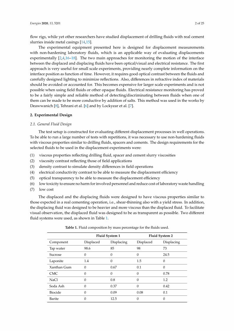
The displaced and the displacing fluids were designed to have viscous properties similar tothose expected in a real cementing operation, i.e., shear-thinning also with a yield stress. In addition,the displacing fluid was designed to be heavier and more viscous than the displaced fluid. To facilitatevisual observation, the displaced fluid was designed to be as transparent as possible. Two differentfluid systems were used, as shown in Table 1.

Table 1. Fluid composition by mass percentage for the fluids used.

Fluid System 1 Fluid System 2

Component Displaced Displacing Displaced Displacing

Tap water 98.6 85 98 73

Sucrose 0 0 0 24.5

Laponite 1.4 0 1.5 0

Xanthan Gum 0 0.67 0.1 0

CMC 0 0 0 0.78

NaCl 0 0.8 0 1.2

Soda Ash 0 0.37 0 0.42

Biocide 0 0.09 0.08 0.1

Barite 0 12.5 0 0

Energies 2020, 13, 5201 3 of 25

Barite was used as weight material of the displacing fluid in fluid system 1.However, table sugar (sucrose) was found to suit the test system better and was used to increase thedensity in fluid system 2. Sucrose dissolves in water to give the increased density without the additionof solid particles. Also, as a minor point, sucrose will increase the index of refraction in the fluids,which is also advantageous for visualization. Colouring agents (uranine and methylene blue) wereadded to the displacing fluid in fluid system 2 to improve visual contrast between the fluids. Finally,NaCl was added to the displacing fluid to provide electrical conductivity contrast.

A study of the fluid mechanical basis for conducting laboratory experiments with the scope ofpresenting displacement results that are relevant for industrial application concluded that it can bepossible to use laboratory fluids in laboratory test equipment and produce results that can be scaled upto field applications [19]. Occasionally, the casings are rotated in well cementing operations to improvethe displacement. The rotation rates in the laboratory will in general be different than those in the fieldas a result of using different viscous properties along with operating in a different geometry.

2.2. Test Rig

2.2.1. Overview

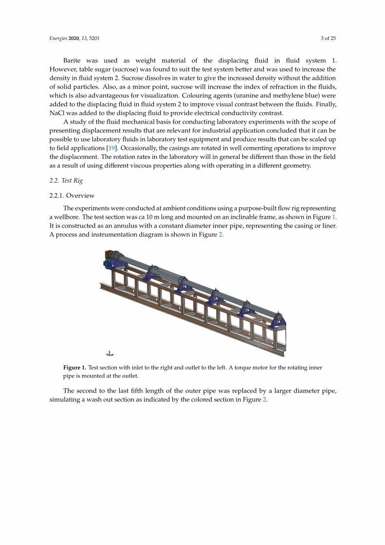
The experiments were conducted at ambient conditions using a purpose-built flow rig representinga wellbore. The test section was ca 10 m long and mounted on an inclinable frame, as shown in Figure 1.It is constructed as an annulus with a constant diameter inner pipe, representing the casing or liner.A process and instrumentation diagram is shown in Figure 2.

Energies 2020, 13, x FOR PEER REVIEW 3 of 26

Barite was used as weight material of the displacing fluid in fluid system 1. However, table sugar (sucrose) was found to suit the test system better and was used to increase the density in fluid system 2. Sucrose dissolves in water to give the increased density without the addition of solid particles. Also, as a minor point, sucrose will increase the index of refraction in the fluids, which is also advantageous for visualization. Colouring agents (uranine and methylene blue) were added to the displacing fluid in fluid system 2 to improve visual contrast between the fluids. Finally, NaCl was added to the displacing fluid to provide electrical conductivity contrast.

A study of the fluid mechanical basis for conducting laboratory experiments with the scope of presenting displacement results that are relevant for industrial application concluded that it can be possible to use laboratory fluids in laboratory test equipment and produce results that can be scaled up to field applications [19]. Occasionally, the casings are rotated in well cementing operations to improve the displacement. The rotation rates in the laboratory will in general be different than those in the field as a result of using different viscous properties along with operating in a different geometry.

2.2. Test Rig

2.2.1. Overview

The experiments were conducted at ambient conditions using a purpose-built flow rig representing a wellbore. The test section was ca 10 m long and mounted on an inclinable frame, as shown in Figure 1. It is constructed as an annulus with a constant diameter inner pipe, representing the casing or liner. A process and instrumentation diagram is shown in Figure 2.

Figure 1. Test section with inlet to the right and outlet to the left. A torque motor for the rotating inner pipe is mounted at the outlet.

The second to the last fifth length of the outer pipe was replaced by a larger diameter pipe, simulating a wash out section as indicated by the colored section in Figure 2.

Figure 1. Test section with inlet to the right and outlet to the left. A torque motor for the rotating innerpipe is mounted at the outlet.

The second to the last fifth length of the outer pipe was replaced by a larger diameter pipe,simulating a wash out section as indicated by the colored section in Figure 2.

Energies 2020, 13, 5201 4 of 25


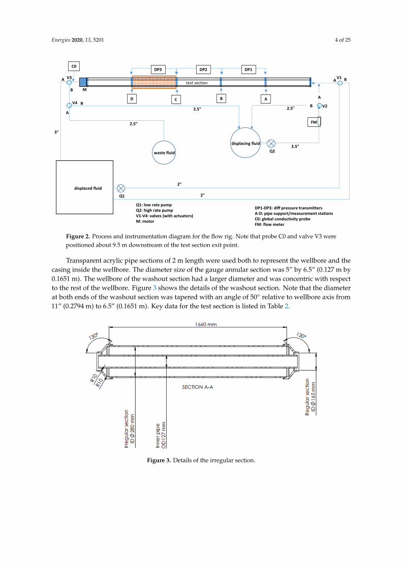
Figure 2. Process and instrumentation diagram for the flow rig. Note that probe C0 and valve V3 were positioned about 9.5 m downstream of the test section exit point.

Transparent acrylic pipe sections of 2 m length were used both to represent the wellbore and the casing inside the wellbore. The diameter size of the gauge annular section was 5” by 6.5” (0.127 m by 0.1651 m). The wellbore of the washout section had a larger diameter and was concentric with respect to the rest of the wellbore. Figure 3 shows the details of the washout section. Note that the diameter at both ends of the washout section was tapered with an angle of 50° relative to wellbore axis from 11” (0.2794 m) to 6.5” (0.1651 m). Key data for the test section is listed in Table 2.

Figure 3. Details of the irregular section.

Table 2. Flow rig key parameters (see Figure 2).

Parameter Symbol Value Total length of test section (ca) Ltot 10 m Inner diameter of annulus (outer diameter of inner pipe) Di 0.127 m (5”) Inner diameter of gauge outer pipe Do 0.1651 m (6.5”) Inner diameter of washout section Dwo 0.2794 m (11”) Length of each pipe section Ls 1.920 m Full bore length of washout section Lwo1 1.660 m Length of increased diameter washout section Lwo2 1.805 m Eccentricity ε 0 and-0.42

waste fluid

V4

V3

C0

ABCD

V1

displacing fluid

3"

displaced fluid2"

Q1

Q2

FM

V2

2.5"

2.5"

2.5"

2.5"

Q1: low rate pumpQ2: high rate pumpV1-V4: valves (with actuators)M: motor

DP1-DP3: diff pressure transmittersA-D: pipe support/measurement stationsC0: global conductivity probeFM: flow meter

Mtest section

DP3 DP2 DP1

BA

B

A

2"

B

A

B

A

Figure 2. Process and instrumentation diagram for the flow rig. Note that probe C0 and valve V3 werepositioned about 9.5 m downstream of the test section exit point.

Transparent acrylic pipe sections of 2 m length were used both to represent the wellbore and thecasing inside the wellbore. The diameter size of the gauge annular section was 5” by 6.5” (0.127 m by0.1651 m). The wellbore of the washout section had a larger diameter and was concentric with respectto the rest of the wellbore. Figure 3 shows the details of the washout section. Note that the diameterat both ends of the washout section was tapered with an angle of 50◦ relative to wellbore axis from11” (0.2794 m) to 6.5” (0.1651 m). Key data for the test section is listed in Table 2.


Figure 2. Process and instrumentation diagram for the flow rig. Note that probe C0 and valve V3 were positioned about 9.5 m downstream of the test section exit point.

Transparent acrylic pipe sections of 2 m length were used both to represent the wellbore and the casing inside the wellbore. The diameter size of the gauge annular section was 5” by 6.5” (0.127 m by 0.1651 m). The wellbore of the washout section had a larger diameter and was concentric with respect to the rest of the wellbore. Figure 3 shows the details of the washout section. Note that the diameter at both ends of the washout section was tapered with an angle of 50° relative to wellbore axis from 11” (0.2794 m) to 6.5” (0.1651 m). Key data for the test section is listed in Table 2.



Parameter Symbol Value Total length of test section (ca) Ltot 10 m Inner diameter of annulus (outer diameter of inner pipe) Di 0.127 m (5”) Inner diameter of gauge outer pipe Do 0.1651 m (6.5”) Inner diameter of washout section Dwo 0.2794 m (11”) Length of each pipe section Ls 1.920 m Full bore length of washout section Lwo1 1.660 m Length of increased diameter washout section Lwo2 1.805 m Eccentricity ε 0 and-0.42

waste fluid

V4

V3

C0

ABCD

V1

displacing fluid

3"

displaced fluid2"

Q1

Q2

FM

V2

2.5"

2.5"

2.5"

2.5"

Q1: low rate pumpQ2: high rate pumpV1-V4: valves (with actuators)M: motor

DP1-DP3: diff pressure transmittersA-D: pipe support/measurement stationsC0: global conductivity probeFM: flow meter

Mtest section

DP3 DP2 DP1

BA

B

A

2"

B

A

B

A


Energies 2020, 13, 5201 5 of 25


Parameter Symbol Value

Total length of test section (ca) Ltot 10 mInner diameter of annulus (outer diameter of inner pipe) Di 0.127 m (5”)Inner diameter of gauge outer pipe Do 0.1651 m (6.5”)Inner diameter of washout section Dwo 0.2794 m (11”)Length of each pipe section Ls 1.920 mFull bore length of washout section Lwo1 1.660 mLength of increased diameter washout section Lwo2 1.805 mEccentricity ε 0 and −0.42

The inner pipe was supported by bearing joints (see Figure 4) every 2 m at the wellbore sectionconnections to prevent inner pipe sagging. The bearing joint consists of an outer flange supporting theouter pipe, an inner pipe bearing set to support the inner pipe and to transmit torque between sectionsof inner pipe, and bolts to fix the inner pipe bearing laterally and to allow adjustment of eccentricity.The bolts each have a diameter of 10 mm. This represents about 4.4% of the cross-section area of theannulus and is thus expected to have a minimal impact on the flow and displacement.Energies 2020, 13, x FOR PEER REVIEW 5 of 26

Figure 4. Bearing joint connecting two sections of inner pipe.

The inner pipe was supported by bearing joints (see Figure 4) every 2 m at the wellbore section connections to prevent inner pipe sagging. The bearing joint consists of an outer flange supporting the outer pipe, an inner pipe bearing set to support the inner pipe and to transmit torque between sections of inner pipe, and bolts to fix the inner pipe bearing laterally and to allow adjustment of eccentricity. The bolts each have a diameter of 10 mm. This represents about 4.4% of the cross-section area of the annulus and is thus expected to have a minimal impact on the flow and displacement.

The inner pipe was also mounted to a torque motor at the downstream end, allowing rotation of the inner pipe at a controlled rate. The eccentricity ε of the inner pipe, defined as the offset of the inner pipe axis relative to the wellbore axis divided by the concentric annular gap, could be adjusted manually using screws at the joints. Experiments were conducted with eccentricities of ε = 0 and ε = −0.42, with negative values for inner pipe axis below the wellbore axis.

The displaced and displacing fluid were stored in separate tanks prior to the experiments (see Figure 2). Within each tank there was a thermostat-controlled heating element to keep the temperature of the fluids at a temperature slightly above ambient temperature. Two valves at the flow loop inlet, see Figure 5, were used to select the source of flow through the test section being either displaced or displacing fluid.

Figure 5. Piping and valves at inlet to test section. The valves V1 and V2 of Figure 2 were controlled from the PC using pneumatic actuators. A drain valve (blue handle) with corresponding hose (not shown in Figure 2) was used to drain the test section after an experiment.


The inner pipe was also mounted to a torque motor at the downstream end, allowing rotationof the inner pipe at a controlled rate. The eccentricity ε of the inner pipe, defined as the offset of theinner pipe axis relative to the wellbore axis divided by the concentric annular gap, could be adjustedmanually using screws at the joints. Experiments were conducted with eccentricities of ε = 0 andε = −0.42, with negative values for inner pipe axis below the wellbore axis.

The displaced and displacing fluid were stored in separate tanks prior to the experiments(see Figure 2). Within each tank there was a thermostat-controlled heating element to keep thetemperature of the fluids at a temperature slightly above ambient temperature. Two valves at the flowloop inlet, see Figure 5, were used to select the source of flow through the test section being eitherdisplaced or displacing fluid.

Energies 2020, 13, 5201 6 of 25



The inner pipe was supported by bearing joints (see Figure 4) every 2 m at the wellbore section connections to prevent inner pipe sagging. The bearing joint consists of an outer flange supporting the outer pipe, an inner pipe bearing set to support the inner pipe and to transmit torque between sections of inner pipe, and bolts to fix the inner pipe bearing laterally and to allow adjustment of eccentricity. The bolts each have a diameter of 10 mm. This represents about 4.4% of the cross-section area of the annulus and is thus expected to have a minimal impact on the flow and displacement.

The inner pipe was also mounted to a torque motor at the downstream end, allowing rotation of the inner pipe at a controlled rate. The eccentricity ε of the inner pipe, defined as the offset of the inner pipe axis relative to the wellbore axis divided by the concentric annular gap, could be adjusted manually using screws at the joints. Experiments were conducted with eccentricities of ε = 0 and ε = −0.42, with negative values for inner pipe axis below the wellbore axis.

The displaced and displacing fluid were stored in separate tanks prior to the experiments (see Figure 2). Within each tank there was a thermostat-controlled heating element to keep the temperature of the fluids at a temperature slightly above ambient temperature. Two valves at the flow loop inlet, see Figure 5, were used to select the source of flow through the test section being either displaced or displacing fluid.

Figure 5. Piping and valves at inlet to test section. The valves V1 and V2 of Figure 2 were controlled from the PC using pneumatic actuators. A drain valve (blue handle) with corresponding hose (not shown in Figure 2) was used to drain the test section after an experiment.

Figure 5. Piping and valves at inlet to test section. The valves V1 and V2 of Figure 2 were controlled fromthe PC using pneumatic actuators. A drain valve (blue handle) with corresponding hose (not shown inFigure 2) was used to drain the test section after an experiment.

In Figure 5 it is seen that the fluid makes a 90 degree turn at the inlet. This does not provideoptimal inlet flow conditions, in particular for fluids with elasticity. We did not measure the elasticproperties of the fluids used in this setup. However, we have not noticed any clear indications that theinlet bend has affected the results.

2.2.2. Instrumentation

The flow rate was measured using am Optiflux 4000 electromagnetic flow meter (Krohne, Duisburg,Germany) that was mounted downstream of the main pump Q2 as shown in Figure 2. To measurethe pressure losses along the annulus, three differential pressure (DP) cells of type Fuji were used,see Table 3. These measured the differential pressure across three sequential 2 m sections of thetest section. The pressure cell DP1 was used for measuring the gauge hole annular pressure losses.The other two DP cells had one or two pressure outlets mounted near the washout section and thecorresponding pressure measurements were affected by the diameter changes at the ends of thewashout section. It turned out that DP3 was faulty and no data are available from this sensor.

Table 3. Differential pressure transmitters.

Name Type Position

DP1 (DP10) Fuji FCX, Type FKCW35V2AXAYYAE, Range-130 to130 kPa Between 2 m and 4 m from inlet

DP2 (DP4) Fuji FCX-AII, Type FKCW35V4AXCYYAE, Range-130to 130 kPa Between 4 m and 6 m from inlet

DP3 (DP1) Fuji FCX, Type FKCW43V2-AXCYY-AF, Range-32 kPato +32 kPa.

Between 6 m and 8 m from inlet(across irregular section)

The location of the pressure ports were azimuthally between probes 6 and 7, and axially at thesame position as the conductivity probes, with two of the ports shared between neighboring DP cells.

The propagation of the displacing fluid was monitored using conductivity probes, each consistingof a pair of electrodes. For each probe the conductivity between the electrodes was measured.24 conductivity probes were located at four different axial stations along the test section (stations A, B,C and D in Figure 2). Six of eight slots for conductivity probes were used at each station; slots 2 and 4were installed but not used in measurements (Figure 6). The number of actual probes was limited bythe number of available channels of the amplifier. Note that no measurement, except visual, could be

Energies 2020, 13, 5201 7 of 25

conducted in the wash out section. Here the measurement probes were positioned immediatelyupstream and downstream this section.


In Figure 5 it is seen that the fluid makes a 90 degree turn at the inlet. This does not provide optimal inlet flow conditions, in particular for fluids with elasticity. We did not measure the elastic properties of the fluids used in this setup. However, we have not noticed any clear indications that the inlet bend has affected the results.

2.2.2. Instrumentation

The flow rate was measured using am Optiflux 4000 electromagnetic flow meter (Krohne, Duisburg, Germany) that was mounted downstream of the main pump Q2 as shown in Figure 2. To measure the pressure losses along the annulus, three differential pressure (DP) cells of type Fuji were used, see Table 3. These measured the differential pressure across three sequential 2 m sections of the test section. The pressure cell DP1 was used for measuring the gauge hole annular pressure losses. The other two DP cells had one or two pressure outlets mounted near the washout section and the corresponding pressure measurements were affected by the diameter changes at the ends of the washout section. It turned out that DP3 was faulty and no data are available from this sensor.

The location of the pressure ports were azimuthally between probes 6 and 7, and axially at the same position as the conductivity probes, with two of the ports shared between neighboring DP cells.

Table 3. Differential pressure transmitters.

Name Type Position DP1 (DP10)

Fuji FCX, Type FKCW35V2AXAYYAE, Range-130 to 130 kPa

Between 2 m and 4 m from inlet

DP2 (DP4)

Fuji FCX-AII, Type FKCW35V4AXCYYAE, Range-130 to 130 kPa

Between 4 m and 6 m from inlet

DP3 (DP1)

Fuji FCX, Type FKCW43V2-AXCYY-AF, Range-32 kPa to +32 kPa.

Between 6 m and 8 m from inlet (across irregular section)

The propagation of the displacing fluid was monitored using conductivity probes, each consisting of a pair of electrodes. For each probe the conductivity between the electrodes was measured. 24 conductivity probes were located at four different axial stations along the test section (stations A, B, C and D in Figure 2). Six of eight slots for conductivity probes were used at each station; slots 2 and 4 were installed but not used in measurements (Figure 6). The number of actual probes was limited by the number of available channels of the amplifier. Note that no measurement, except visual, could be conducted in the wash out section. Here the measurement probes were positioned immediately upstream and downstream this section.

Figure 6. Schematic cross section of test section showing position of conductivity probes and inner pipe in eccentric position. Pressure ports (not shown) were located between probes 6 and 7.

Figure 6. Schematic cross section of test section showing position of conductivity probes and innerpipe in eccentric position. Pressure ports (not shown) were located between probes 6 and 7.

Each conductivity probe consisted of a pair of 3 mm diameter steel screws which were directedradially into the annulus and positioned 8 mm apart (center-center distance). Thus, the gap between theelectrodes was 5 mm. In order to reduce any effects of the flow disturbance caused by the electrodes onthe measurements, the electrodes in each pair were mounted at the same axial position, i.e., separatedin the azimuthal direction. The penetration depth was 5 mm, while the width of the concentric annuluswas ca 19 mm. Thus, the electrodes covered about one quarter of the radial distance in concentricannulus configuration.

The conductivity probes were connected to a signal amplifier which was specially designed for usewith conductivity probes for measuring water wave heights (Wave Amplifier type 108, DHI, Hørsholm,Denmark). This amplifier gives an electrical AC signal around 2750 Hz. The resistance λ per unitlength between a pair of infinitely long parallel cylindrical electrodes of common diameter δ, is givenas shown in Equation (1) [20]:

λ =ψ

πcosh−1

(∆δ

)(1)

where ψ is the resistivity of the fluid around the electrodes and ∆ is their center-center distance.The geometrical factor of Equation (1) thus changes by 8% with an increase in distance ∆ from 7.5 mmto 8.5 mm. Since the electrodes do not span the entire annular gap, a key question is to what extentthey will detect conducting fluid which is not in direct contact with the electrodes. The measurementprinciple is illustrated in Figure 7. As the displacement process progresses, the contact with thehigh conductivity fluid increases and a general increase in conductivity is measured. In this case,which is representative for the displacement experiments with concentric annulus, the displaced fluidis stratified above the displacing fluid due to lower density. The interface is here strongly inclinedwith respect to the cross-section plane, and almost parallel to the wellbore axis. Thus the length ofelectrode contacting the conducting fluid increases with time as the thickness of the displaced fluid layerdiminished. This gives a fairly slow transition from minimum to maximum conductivity. When theinterface is nearly normal to the wellbore axis, and thus parallel to the electrode axes, the transitionfrom minimum to maximum conductivity will be much more abrupt, unless there is strong mixingbetween the fluids.

Energies 2020, 13, 5201 8 of 25


Each conductivity probe consisted of a pair of 3 mm diameter steel screws which were directed radially into the annulus and positioned 8 mm apart (center-center distance). Thus, the gap between the electrodes was 5 mm. In order to reduce any effects of the flow disturbance caused by the electrodes on the measurements, the electrodes in each pair were mounted at the same axial position, i.e., separated in the azimuthal direction. The penetration depth was 5 mm, while the width of the concentric annulus was ca 19 mm. Thus, the electrodes covered about one quarter of the radial distance in concentric annulus configuration.

The conductivity probes were connected to a signal amplifier which was specially designed for use with conductivity probes for measuring water wave heights (Wave Amplifier type 108, DHI, Hørsholm, Denmark). This amplifier gives an electrical AC signal around 2750 Hz. The resistance λ per unit length between a pair of infinitely long parallel cylindrical electrodes of common diameter δ, is given as shown in Equation (1) [20]:

1coshψλπ δ

− Δ =

(1)

where ψ is the resistivity of the fluid around the electrodes and Δ is their center-center distance. The geometrical factor of Equation (1) thus changes by 8% with an increase in distance Δ from 7.5 mm to 8.5 mm. Since the electrodes do not span the entire annular gap, a key question is to what extent they will detect conducting fluid which is not in direct contact with the electrodes. The measurement principle is illustrated in Figure 7. As the displacement process progresses, the contact with the high conductivity fluid increases and a general increase in conductivity is measured. In this case, which is representative for the displacement experiments with concentric annulus, the displaced fluid is stratified above the displacing fluid due to lower density. The interface is here strongly inclined with respect to the cross-section plane, and almost parallel to the wellbore axis. Thus the length of electrode contacting the conducting fluid increases with time as the thickness of the displaced fluid layer diminished. This gives a fairly slow transition from minimum to maximum conductivity. When the interface is nearly normal to the wellbore axis, and thus parallel to the electrode axes, the transition from minimum to maximum conductivity will be much more abrupt, unless there is strong mixing between the fluids.

Figure 7. Principle of operation for conductivity measurement. Lower density displaced fluid (yellow) stratified above higher density displacing fluid (blue).

Except for an offset value, the measured voltage signal, Vo, is proportional to the average conductance G between the electrodes. Assuming that boundary effects can be ignored, the conductance G is proportional to the length Lp of the electrodes of a probe, i.e.:

Figure 7. Principle of operation for conductivity measurement. Lower density displaced fluid (yellow)stratified above higher density displacing fluid (blue).

Except for an offset value, the measured voltage signal, Vo, is proportional to the averageconductance G between the electrodes. Assuming that boundary effects can be ignored, the conductanceG is proportional to the length Lp of the electrodes of a probe, i.e.:

G =Lp

λ=

πσLp

cosh−1(

∆δ

) (2)

where σ ≡ 1/ψ is the fluid conductivity. The conductivity increases with increasing length of probebeing immersed in the high conductive fluid.

The wave amplifier ensures that the voltage across the electrodes is constant; being independentof the conductance between the electrodes. Instead, a change in the conductance will result in a changein the amplification in the wave amplifier, and thus a change in the output voltage. Thus, accountingfor any voltage offset we may write the measured voltage signal as given in Equation (3):

Vo = Vo f f set + K G (3)

where K is a gain factor of the measurement system.Both the displaced and the displacing fluids have some conductivity. However, the conductivity

of the displaced fluid is an order of magnitude smaller than that of the displacing fluid, and we mayapproximate it as being non-conducting. The conductivity probe signal response will partly be due tochanges in the local conductivity, σ, due to fluid mixing, and partly due to the position of the interfacebetween low and high conductivity fluid relative to the probes.

The measured voltage for each pair of electrodes will vary between a minimum value Vo,mincorresponding to the displaced fluid with conductivity Gmin and a maximum value Vo,max correspondingto the displacing fluid with conductivity Gmax. Assuming linearity between conductivity and volumefraction of displacing (high-conductivity) fluid we have:

G = φGmax + (1−φ)Gmin (4)

Using Equation (3) we then obtain:

φ =G−Gmin

Gmax −Gmin=

Vo −Vo,min

Vo,max −Vo,min≡ Vr (5)

Equation (5) holds true for a homogeneous mixture of the two fluids, and is also expected to holdtrue in some average sense for a heterogeneous system where there is a macroscopic interface betweenthe two fluids.

Energies 2020, 13, 5201 9 of 25

Although a given value of φ can be obtained from this expression both from a homogeneousmixture of two fluids and from a given configuration of a sharp interface between the same fluids,we may distinguish between these two cases by considering the time derivative of the signal Vo(t).A section with mixing will yield a lesser pronounced change of the signal with time than a sharpdisplacement front.

Let S be the total fluid domain around a pair of electrodes. Let further φ(r) be the localvolume fraction of displacing fluid and define an interface ∂Si between displaced and displacing fluidby φ(r) = 0.5. Although the fluids in the experiments were miscible (both were water-based), we assumethat the interface was fairly well defined through each displacement experiment, since the duration ofeach experiment (on the order of one minute) is short relative to the time for molecular diffusion overa typical length scale (annular gap width). The fluid-fluid interface may become convoluted due toconvective processes driven by gravity or hydrodynamic instabilities, but microscopic mixing of thefluids before the washout is expected to be primarily due to turbulence in the entrance region to thetest section.

Since Maxwell’s equations are linear, we postulate that the normalized signal response Vr willnot depend on the absolute values of the conductivities. We also postulate that it will depend onlyweakly on the shape of the wall interface ∂Sw of ∂S = ∂Sw + ∂Si, where ∂S is the total boundary of thefluid domain. We here ignore the inlets and outlets of the test section, which are both far removedfrom the conductivity probe electrodes. Thus, we conclude that Vr almost exclusively depends on thedistribution φ(r) and, assuming there is little mixing between the fluids, mainly on the interface ∂Si.Note that this interface is not necessarily simply connected, a well-defined fluid front. For example,there may be isolated pockets of bypassed displaced fluid. If, however, the interface ∂Si is a well-definedfluid front, separating the displaced and displacing fluids axially, we expect that the signal response Vr

will be a monotonous function of the axial position of this displacement front.An additional conductivity probe, type CTI-500 (Jumo, Fulda, Germany, hereafter called C0),

was mounted on a spool section in the fluid outlet downstream of the test section. The spool wasconnected to the test section with a 2.5” flexible hose of length approximately 9.5 m. The probe is acombined inductive conductivity and temperature transmitter and measured the electrical conductivityand the temperature of the fluid which had exited the test section. From the measured conductivity thevolume fraction of the conducting fluid and thus the overall efficiency of the displacement process canbe determined. There was no special mixing element upstream of the probe C0. However, it is assumedthat the two fluids were well mixed in the transversal plane at the location of the C0, both because ofthe length of the connecting flexible hose, the higher fluid velocity in the hose (1.38 m/s), and becauseof the change in flow direction at the outlet of the test section.

The objectives of the measurements with the conductivity probes were three-fold:

(1) detect the arrival of the displacing fluid at a particular probe location at the corresponding timewhere the signal Vr changes from low to high

(2) assess qualitatively the degree of mixing of the two fluids at the probe location by measuring theduration of the transition from low to high signal level

(3) measure and quantify the concentration of displacing fluid at the probe location

For the two first objectives it is only necessary to assume that the measured signal is a monotonouslyincreasing function of the relative fraction φ of displacing fluid and that the two fluids have sufficientlylarge conductivity contrast. These were the main objectives of the distributed conductivity probes.The third objective requires a known relationship between the measured signal and the volumeconcentration of the displacing fluid and that the concentration is uniform in the sampling volume ofthe probe. In the present experiments the concentration of electrolyte, NaCl, in the displacing fluidwas so low that a linear relationship can be assumed, as discussed below.

Since the scope of the measurements is to determine the displacement fluid volume fraction φrather than the effective conductance G between the electrodes, we will in the following work only

Energies 2020, 13, 5201 10 of 25

with the normalized probe response Vr. Since the absolute value V0 of each probe was not critical,the probes were not calibrated to give the same value for the same fluid (displaced and displacing).The offset and gain factors for each channel of the signal amplifier were adjusted prior to conductingthe experiments to avoid saturation of the signal; meaning being out of range. Still this has happenedin a few cases.

The linearity of φ(G) (see Equation (5)) was checked before the experiments by measuring theconductivity of a mixture of a non-conductive and a conductive water-based fluid. Thus, two prototypefluids A0 (water with 1.4% by weight of the (synthetic) clay laponite) and B0 (water with 0.8% by weightxanthan biopolymer and 1.0% by weight NaCl) were mixed in different ratios and the conductivity wasmeasured using a handheld conductivity probe (Hanna Instruments HI933000). The results are shownin Figure 8. The measurement points indicate a linear relationship between conductivity and volumefraction, as shown by the stippled line. For such a mixture the conductivity is proportional to thevolume concentration of the electrolytic ions when the concentration is sufficiently low. Note that thefluids A0 and B0 were not used in the actual displacement experiments, but represent fluid system 1,except for the omission of barite, soda ash and biocide in the displacing fluid. This omission is notexpected to have any impact on the linearity of the conductivity versus composition.Energies 2020, 13, x FOR PEER REVIEW 10 of 26

Figure 8. Measured conductivity (points) versus volume fraction of fluid B0. Stippled line shows the linear regression of the measurement points.

While conducting the experiments, the following data were logged 50 times per second:

• Flow rate (FM) • Differential pressure (DP1, DP2, DP3) • Inner pipe rotation speed (RPM) • Mixed fluid conductivity downstream test section (probe C0) • Mixed fluid temperature downstream test section (probe T0) • Tank temperature of displacing fluid (probe T1) • Local conductivity at stations A, B, C and D (probes Aj, Bj, Cj, Dj with j = 1, 3, 5, 6, 7, 8)

The displacement process was also set up to be monitored visually using six low-cost web-cameras mounted along the test section as indicated in Table 4.

Table 4. Video camera positions.

Camera Position 1 Section 2 (between stations A and B), vertical view from bottom 2 Section 2 (between stations A and B), side view 3 Section 3 (between stations B and C), side view 4 Section 4 (washout section, between stations C and D), vertical view from bottom 5 Section 4 (washout section, between stations C and D), side view 6 Section 5 (after station D), side view

Fluids were also characterized in terms of electrical conductivity using a HI933000 handheld conductivity probe (Hanna Instruments, Woonsocket, RI, USA). In addition, the pH was frequently measured. To keep the volume of test fluids at a minimum, as much as possible was reused. Therefore, there would always be a little degree of contamination of the fluids with the other fluid. As seen in Figure 9, the conductivity of the displaced fluid increased over time, while the conductivity of the displacing fluid was more stable. Still the contrast is sufficiently large to be able to measure the displacement properly.

y = 13.955x + 0.7043

0

2

4

6

8

10

12

14

16

0 0.2 0.4 0.6 0.8 1

Cond

uctiv

ity [m

S/cm

]

φ = Volume fraction fluid B0 (displacing fluid)

Range 2:Fluid to waste tank

Range 3:Fluid to displacement tank

Range 1:Fluid to displaced tank

Figure 8. Measured conductivity (points) versus volume fraction of fluid B0. Stippled line shows thelinear regression of the measurement points.

While conducting the experiments, the following data were logged 50 times per second:

• Flow rate (FM)• Differential pressure (DP1, DP2, DP3)• Inner pipe rotation speed (RPM)• Mixed fluid conductivity downstream test section (probe C0)• Mixed fluid temperature downstream test section (probe T0)• Tank temperature of displacing fluid (probe T1)• Local conductivity at stations A, B, C and D (probes Aj, Bj, Cj, Dj with j = 1, 3, 5, 6, 7, 8)

The displacement process was also set up to be monitored visually using six low-cost web-camerasmounted along the test section as indicated in Table 4.

Energies 2020, 13, 5201 11 of 25

Table 4. Video camera positions.

Camera Position

1 Section 2 (between stations A and B), vertical view from bottom2 Section 2 (between stations A and B), side view3 Section 3 (between stations B and C), side view

4 Section 4 (washout section, between stations C and D), vertical view from bottom5 Section 4 (washout section, between stations C and D), side view6 Section 5 (after station D), side view

Fluids were also characterized in terms of electrical conductivity using a HI933000 handheldconductivity probe (Hanna Instruments, Woonsocket, RI, USA). In addition, the pH was frequentlymeasured. To keep the volume of test fluids at a minimum, as much as possible was reused. Therefore,there would always be a little degree of contamination of the fluids with the other fluid. As seenin Figure 9, the conductivity of the displaced fluid increased over time, while the conductivity ofthe displacing fluid was more stable. Still the contrast is sufficiently large to be able to measure thedisplacement properly.Energies 2020, 13, x FOR PEER REVIEW 11 of 26

Figure 9. Fluid conductivity measured during 10 consecutive displacement experiments using the conductivity probe C0.

2.3. Test Procedures

A detailed test procedure was established for running the experiments. The physical items in the test procedure are illustrated in Figure 3. The test procedure is as follows:

1) Prepare data logging program: a) check/set appropriate limit values for conductivity probe C0 (see Figure 8). These values

control the outlet valves. b) check/set correct flow rate value (0.00436 m3/s, corresponding to 0.5 m/s in the regular size

annulus)). 2) Start data logging 3) Start circulation of fluids with displaced fluid circulating in the test section and displacing fluid

circulating in the bypass line. 4) Take sample of displaced fluid. 5) Flush DP cells with displaced fluid. 6) Stop circulation of displaced fluid for zero DP measurements. 7) Restart circulation of displaced fluid. 8) Turn on video lights and start video recording 9) Start displacement experiment by switching to displacing fluid using computer-controlled valve 10) Switch to automatic outlet valve control mode in logging program 11) Stop video recordings when outlet valves have switched to position 3 (displacing fluid) 12) Continue circulation with displacing fluid for at least one minute after stopping experiment. 13) Take sample of displacing fluid 14) Stop circulation

3. Data evaluation and Processing

3.1. Pressure Drop Measurements

The pressure gradient values were logged as indicated in Figure 2. The viscosity flow curves were measured using a manual six speed Fann35 viscometer and the fluid viscosity is described reasonably well using the Herschel-Bulkley model. The model parameter values for the fluid are shown in Table 5 together with calculated values for Reynolds number and pressure gradient for concentric and eccentric casing. In the table the surplus stress τs is a Herschel-Bulkley parameter following Saasen & Ytrehus [21], and is defined as:

Figure 9. Fluid conductivity measured during 10 consecutive displacement experiments using theconductivity probe C0.

2.3. Test Procedures

A detailed test procedure was established for running the experiments. The physical items in thetest procedure are illustrated in Figure 3. The test procedure is as follows:

(1) Prepare data logging program:

(a) check/set appropriate limit values for conductivity probe C0 (see Figure 8). These valuescontrol the outlet valves.

(b) check/set correct flow rate value (0.00436 m3/s, corresponding to 0.5 m/s in the regular sizeannulus)).

(2) Start data logging(3) Start circulation of fluids with displaced fluid circulating in the test section and displacing fluid

circulating in the bypass line.

Energies 2020, 13, 5201 12 of 25

(4) Take sample of displaced fluid.(5) Flush DP cells with displaced fluid.(6) Stop circulation of displaced fluid for zero DP measurements.(7) Restart circulation of displaced fluid.(8) Turn on video lights and start video recording(9) Start displacement experiment by switching to displacing fluid using computer-controlled valve(10) Switch to automatic outlet valve control mode in logging program(11) Stop video recordings when outlet valves have switched to position 3 (displacing fluid)(12) Continue circulation with displacing fluid for at least one minute after stopping experiment.(13) Take sample of displacing fluid(14) Stop circulation

3. Data evaluation and Processing

3.1. Pressure Drop Measurements

The pressure gradient values were logged as indicated in Figure 2. The viscosity flow curves weremeasured using a manual six speed Fann35 viscometer and the fluid viscosity is described reasonablywell using the Herschel-Bulkley model. The model parameter values for the fluid are shown inTable 5 together with calculated values for Reynolds number and pressure gradient for concentric andeccentric casing. In the table the surplus stress τs is a Herschel-Bulkley parameter following Saasen &Ytrehus [21], and is defined as:

τs = τ( .γs

)− τy (6)

where.γs is a shear rate which is characteristic for the flow. τ

( .γs

)is interpolated from the Fann

measurements. The characteristic shear rate,.γs, is defined as

.γs =

12UDo −Di

= 158 s−1 (7)

where U is the average fluid velocity in the regular section. The surplus stress is presented to visualizethe viscosity difference at the shear rates relevant for the fluid flow.

Table 5. Transport properties for the barite free two-fluid systems.

Properties Displaced Displacing

Fluid density ρ (kg/m3) 1000 1100Yield stress τy (Pa) 4.9 1.8Consistency index K (Pa.sn) 0.47 0.87Fluid flow index n (-) 0.55 0.57Surplus stress τs (Pa) @

.γs = 158 s-1 7.2 15.3

Reynolds number @ U = 0.5 m/s (-) 199 164Pressure gradient @ U = 0.5 m/s (Pa/m) (eccentric/concentric) 1293/1580 1729/2108

3.2. Pump Rate Variability

The delivered power to the pump was adjusted automatically in order to maintain constantflowrate as the fluid source is switched from displaced fluid to displacing fluid. Initially there wereunacceptably large fluctuations in the flow rate adjustments. Before finishing the development of theset-up, the flow rate control was improved, leading to much smaller fluctuations. Figure 10 shows thenormalized flow rates versus times for the experiments after the improved algorithm was implemented.

Energies 2020, 13, 5201 13 of 25


( )s s yτ τ γ τ= − (6)

where sγ is a shear rate which is characteristic for the flow. ( )sτ γ is interpolated from the Fann

measurements. The characteristic shear rate, sγ , is defined as

112 158so i

U sD D

γ −= =−

(7)

where U is the average fluid velocity in the regular section. The surplus stress is presented to visualize the viscosity difference at the shear rates relevant for the fluid flow.

Table 5. Transport properties for the barite free two-fluid systems.

Properties Displaced Displacing Fluid density ρ (kg/m3) 1000 1100 Yield stress τy (Pa) 4.9 1.8 Consistency index K (Pa.sn) 0.47 0.87 Fluid flow index n (-) 0.55 0.57 Surplus stress τs (Pa) @ sγ = 158 s-1 7.2 15.3

Reynolds number @ U = 0.5 m/s (-) 199 164 Pressure gradient @ U = 0.5 m/s (Pa/m) (eccentric/concentric) 1293/1580 1729/2108

3.2. Pump Rate Variability

The delivered power to the pump was adjusted automatically in order to maintain constant flowrate as the fluid source is switched from displaced fluid to displacing fluid. Initially there were unacceptably large fluctuations in the flow rate adjustments. Before finishing the development of the set-up, the flow rate control was improved, leading to much smaller fluctuations. Figure 10 shows the normalized flow rates versus times for the experiments after the improved algorithm was implemented.

Figure 10. Normalized fluid flow rate versus time from start of displacement for the experiments with the automatic pump control.

Figure 10. Normalized fluid flow rate versus time from start of displacement for the experiments withthe automatic pump control.

3.3. Conductivity Probe Signals

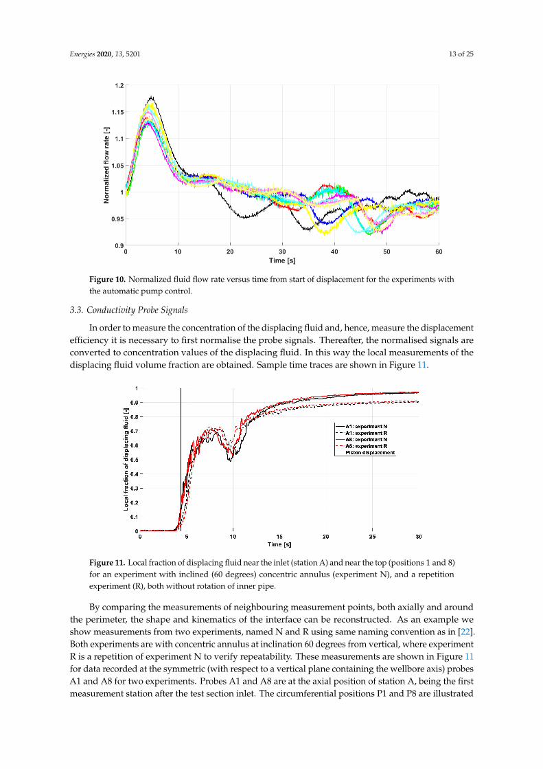
In order to measure the concentration of the displacing fluid and, hence, measure the displacementefficiency it is necessary to first normalise the probe signals. Thereafter, the normalised signals areconverted to concentration values of the displacing fluid. In this way the local measurements of thedisplacing fluid volume fraction are obtained. Sample time traces are shown in Figure 11.


3.3. Conductivity Probe Signals

In order to measure the concentration of the displacing fluid and, hence, measure the displacement efficiency it is necessary to first normalise the probe signals. Thereafter, the normalised signals are converted to concentration values of the displacing fluid. In this way the local measurements of the displacing fluid volume fraction are obtained. Sample time traces are shown in Figure 11.

Figure 11. Local fraction of displacing fluid near the inlet (station A) and near the top (positions 1 and 8) for an experiment with inclined (60 degrees) concentric annulus (experiment N), and a repetitionexperiment (R), both without rotation of inner pipe.

By comparing the measurements of neighbouring measurement points, both axially and around the perimeter, the shape and kinematics of the interface can be reconstructed. As an example we show measurements from two experiments, named N and R using same naming convention as in [22]. Both experiments are with concentric annulus at inclination 60 degrees from vertical, where experiment R is a repetition of experiment N to verify repeatability. These measurements are shown in Figure 11 for data recorded at the symmetric (with respect to a vertical plane containing the wellbore axis) probes A1 and A8 for two experiments. Probes A1 and A8 are at the axial position of station A, being the first measurement station after the test section inlet. The circumferential positions P1 and P8 are illustrated in Figure 6. Since there is no rotation of the inner pipe in these experiments, the signals of A1 and A8 should be equal by symmetry, and a comparison of these also provides a quality check of the data. It is noticed that the symmetry is quite well satisfied, even at later times. Reproducibility is also quite good. However, at later times there is a discrepancy as the displacement in the original experiment seems to be somewhat better than the repetition results. This is anticipated to be caused by the unintentional mixing of the fluids as the fluids are reused.

As discussed above, the conductivity probe signals are assumed to be proportional to the local fraction of displacing fluid at the location of the probe. Although these are only point measurements, they provide an extensive amount of information on the displacement process. We illustrate this by the experimental results shown in Figure 14 where two experiments with horizontal, concentric annulus, without inner pipe rotation are compared, as they represent the simplest experimental conditions. Also, the comparison is interesting, because the viscous properties of the fluids used in the two experiments (A and O) were fairly similar, both in terms of observed pressure drop values and in terms of viscosity measurements. Thus, we expect the results to be similar. In Figure 12 the local fraction of displacing fluid at station A, 2 m from the inlet, is plotted as function of the normalized pump volume (see Equation (13)), thus correcting for any variations in flow rate.

Figure 11. Local fraction of displacing fluid near the inlet (station A) and near the top (positions 1 and 8)for an experiment with inclined (60 degrees) concentric annulus (experiment N), and a repetitionexperiment (R), both without rotation of inner pipe.

By comparing the measurements of neighbouring measurement points, both axially and aroundthe perimeter, the shape and kinematics of the interface can be reconstructed. As an example weshow measurements from two experiments, named N and R using same naming convention as in [22].Both experiments are with concentric annulus at inclination 60 degrees from vertical, where experimentR is a repetition of experiment N to verify repeatability. These measurements are shown in Figure 11for data recorded at the symmetric (with respect to a vertical plane containing the wellbore axis) probesA1 and A8 for two experiments. Probes A1 and A8 are at the axial position of station A, being the firstmeasurement station after the test section inlet. The circumferential positions P1 and P8 are illustrated

Energies 2020, 13, 5201 14 of 25

in Figure 6. Since there is no rotation of the inner pipe in these experiments, the signals of A1 and A8should be equal by symmetry, and a comparison of these also provides a quality check of the data. It isnoticed that the symmetry is quite well satisfied, even at later times. Reproducibility is also quite good.However, at later times there is a discrepancy as the displacement in the original experiment seems tobe somewhat better than the repetition results. This is anticipated to be caused by the unintentionalmixing of the fluids as the fluids are reused.

As discussed above, the conductivity probe signals are assumed to be proportional to the localfraction of displacing fluid at the location of the probe. Although these are only point measurements,they provide an extensive amount of information on the displacement process. We illustrate this by theexperimental results shown in Figure 14 where two experiments with horizontal, concentric annulus,without inner pipe rotation are compared, as they represent the simplest experimental conditions.Also, the comparison is interesting, because the viscous properties of the fluids used in the twoexperiments (A and O) were fairly similar, both in terms of observed pressure drop values and in termsof viscosity measurements. Thus, we expect the results to be similar. In Figure 12 the local fraction ofdisplacing fluid at station A, 2 m from the inlet, is plotted as function of the normalized pump volume(see Equation (13)), thus correcting for any variations in flow rate.Energies 2020, 13, x FOR PEER REVIEW 14 of 26

Figure 12. Displacement versus normalized pump volume for equivalent experiments in Experiments A and O. All measurements were conducted at Station A being 2 m from inlet.

The following information can be obtained from measurement plots like the one shown in Figure 11:

1) The time at which signal value starts increasing indicates when displacing fluid arrives at the different locations (arrival time).

2) The difference in arrival time of signals at different axial positions (stations) but at the same azimuth position can be used to estimate the axial flow velocity of the interface.

3) The steepness of the curves indicates the degree of mixing of displaced and displacing fluid at the location of the probe. A steep transition indicates a well-defined interface with little mixing. A very gradual interface could be due to mixing of the two fluids, but it could also be caused by an interface which is slanted with respect to the axial flow direction.

4) Similarity in shape of probe signals at subsequent axial stations (A, B, C) in the regular section indicates that the displacement front propagates without deformation like a travelling wave. In practice there will always be some distortion, which can be inferred from the differences in shape among the probes.

It is noticed for Experiment O in Figure 12 that in the lower half of the annulus (probes A3, A5 and A6) the displacing fluid arrives sooner than a piston displacement, most likely as an effect of the larger density of the displacing fluid. The vertical line labelled piston displacement corresponds to the time when the total volume of displacing fluid in the test section is equal to the test section volume upstream of station A. For the measurement at the top of the annulus near the top of the annulus (probes A1 and A8) the signals are close to synchronous At the piston displacement time the lower part of the annulus contains about 70% displacing fluid in the O experiment, but only 10–20% displacing fluid in the A experiment. Still, in both experiments the displacing fluid front is seen to be inclined with respect to the pipe axis, since displacing fluid arrives earlier near the bottom of the annulus than near the top.

Video cameras covered the area between the measurement probe arrays and provided valuable supplement to the conductance measurements. Simple videos are more challenging to use for detailed analysis since the interface becomes difficult to track. Particles designed to remain on the fluid-fluid interface could enhance the value of videos. Analysis of the videos alone is difficult to use because of increasing opacity of the fluids, positioning of illumination and reflection of the illuminated light on the pipe wall. Still this method was applicable as additional information to the conductance probe data.

Figure 12. Displacement versus normalized pump volume for equivalent experiments in ExperimentsA and O. All measurements were conducted at Station A being 2 m from inlet.

The following information can be obtained from measurement plots like the one shown inFigure 11:

(1) The time at which signal value starts increasing indicates when displacing fluid arrives at thedifferent locations (arrival time).

(2) The difference in arrival time of signals at different axial positions (stations) but at the sameazimuth position can be used to estimate the axial flow velocity of the interface.

(3) The steepness of the curves indicates the degree of mixing of displaced and displacing fluid atthe location of the probe. A steep transition indicates a well-defined interface with little mixing.A very gradual interface could be due to mixing of the two fluids, but it could also be caused byan interface which is slanted with respect to the axial flow direction.

(4) Similarity in shape of probe signals at subsequent axial stations (A, B, C) in the regular sectionindicates that the displacement front propagates without deformation like a travelling wave.In practice there will always be some distortion, which can be inferred from the differences inshape among the probes.

Energies 2020, 13, 5201 15 of 25

It is noticed for Experiment O in Figure 12 that in the lower half of the annulus (probes A3, A5 andA6) the displacing fluid arrives sooner than a piston displacement, most likely as an effect of the largerdensity of the displacing fluid. The vertical line labelled piston displacement corresponds to the timewhen the total volume of displacing fluid in the test section is equal to the test section volume upstreamof station A. For the measurement at the top of the annulus near the top of the annulus (probes A1 andA8) the signals are close to synchronous At the piston displacement time the lower part of the annuluscontains about 70% displacing fluid in the O experiment, but only 10–20% displacing fluid in the Aexperiment. Still, in both experiments the displacing fluid front is seen to be inclined with respect tothe pipe axis, since displacing fluid arrives earlier near the bottom of the annulus than near the top.

Video cameras covered the area between the measurement probe arrays and provided valuablesupplement to the conductance measurements. Simple videos are more challenging to use for detailedanalysis since the interface becomes difficult to track. Particles designed to remain on the fluid-fluidinterface could enhance the value of videos. Analysis of the videos alone is difficult to use because ofincreasing opacity of the fluids, positioning of illumination and reflection of the illuminated light on thepipe wall. Still this method was applicable as additional information to the conductance probe data.

3.4. Calculation of Displacement Efficiency

We define the displacement efficiency following Deawwanich [8]:

χ(t) = Q·(t−t0)V ; t ≤ tb

χ(t) = Q(tb−t0)+

t∫tb

dt[cA(t)]

V ; t > tb

(8)

where t0 is the time when the displacing fluid enters the test section, V is the annular volume of the testsection, and tb is the time when the first displacing fluid leaves the test section. After the breakthroughtime tb the concentration cA(t) of displaced fluid at the outlet decreases and the displacement efficiencyincreases at a slower rate. As time goes to infinity the displacement efficiency theoretically goes tounity provided no immobilized displaced fluid is left behind. An implicit assumption is that thedisplaced and displacing fluid move with the same velocity, so that the flow rate of the displaced fluidat any location can be written as:

QA(t) = Q(t)cA(t) (9)

In our experiments we did not log the starting time t0 directly. However, we define the startingtime as the time when the inlet valves were switched from pumping displaced fluid to pumpingdisplacing fluid. This time t0 was inferred from the measurements of flow rate and differential pressurein the test section as described in the following. When the inlet valves are switched, a pressure pulsetravels through the test section and there was a transient in the flow rate through the test section.This transient was due to capacity limitations of the pump for the displaced fluid. Before the switchingof the inlet valves the flow in the test section was driven by the pump for the displaced fluid at fullcapacity, which corresponded to a rate somewhat lower than the scheduled rate of the experiment.Thus, at the start of the experiment, corresponding to the switching of the inlet valves the fluid in thetest section was accelerated to the target flow rate. In Figure 10 this is seen as a transient increase in theflowrate as the control of the pump power became over-compensated. Since the flow rate was notconstant, the expression for the displacement efficiency was calculated as:

χ(t) =

t∫tb

dtQ(t)[cA(t)]

VTS(10)

for times t > t0, where VTS is the fluid volume between the inlet point and the conductivity probe C0 atthe outlet and cA is the concentration of displaced fluid at the outlet. We assume, based on the results

Energies 2020, 13, 5201 16 of 25

shown in Figure 8, that the volumetric concentration cA(t) of the displaced fluid at the outlet is a linearfunction of the global conductivity σ0 similarly to the predictions given by Equation (11).

cA(t) =σ0∗(t) − σ0B

σ0A − σ0B(11)

where the conductivities of the displaced and displacing fluids are σ0A and σ0B, and we limit theconcentration to be a number between zero and one:

σ0∗(t) = min(σ0B, max(σ0(t), σ0A)) (12)

These conductivities σ0A and σ0B are calculated by time averages over suitable time intervalsbefore and after the displacement process.

To be applicable for comparison with field operation data it is necessary to plot the displacementefficiency versus normalized pumped volume rather than versus time. Thus, we define the normalizedpumped volume v(t) as independent variable:

v(t) =

t∫t0

dtQ(t)

VTS(13)

We also calculate the breakthrough time, i.e., the time of arrival of first displacing fluid at the outlet.Note, however, that the outlet is defined to be at the location of the conductivity probe, C0, which islocated on a flexible hose about 9.5 m downstream of the annular test section outlet. This distancecorresponds to a volume of ca 30 L with a transit time dependent on the nominal flow rate. Thus,to calculate the breakthrough time at the outlet of the annular section, a flow dependent time valueshould be subtracted from the measured breakthrough time. A corresponding adjustment should thenbe done for the relative breakthrough volume. For some experiments this would give negative valueswhich could be caused by noise in the signal from the global conductivity probe. However, we arehere primarily interested in a relative comparison among the experiments, and not in the absolutevalues of the breakthrough times.

3.5. Reconstruction of Displacement Front Velocity

The axial velocities of the displacement front are reconstructed based on the signals fromconductivity probes along the test section and this was subsequently used to reconstruct the totalfluid flux. Since the latter is also measured, the flux was also used to renormalize the calculated axialvelocities. The calculations are based on a cross correlation of signals from probes at neighbouringmeasurement stations (A, B, C, D) but at the same circumferential position. This approach differsfrom the one used by Renteria et al. [2], who based the calculation on the time t when the signal levelreached 20% of the maximum signal level. The motivation for the present approach was to avoid theuse of an ad hoc signal threshold level.

Using the calculated local velocities, we estimate the total liquid flow rate by numerical integrationover the annular cross section. Since the total liquid flow rate is measured using a Coriolis flow meter,the accuracy of the calculated velocities can be calculated. This accuracy is generally very good.

The cumulative flux of displaced fluid at the different measurement stations are estimated byassuming that the local axial velocities at each station are time-independent and by assuming that theaverage local concentration of displacing fluid is proportional to the normalized signal level. For mostexperiments and most measurement locations, this calculation gives displacement efficiencies beingfar in excess of unity. This indicates that there is a significant velocity difference between the displacedand the displacing fluid. Such a difference can be explained by assuming that the displacing fluidadvances more rapidly in the centre of the annular channel than closer to the wall. Since the probes

Energies 2020, 13, 5201 17 of 25

only protrude 5 mm from the outer wall into the annulus, the signal will be biased towards the fluidpresent at the wall. Although not directly confirmed by experimental observation, the assumptionmentioned above is supported theoretically by the no-slip velocity condition at the wall.

First, we estimate the local axial velocity vi,j at circumferential position i and station j (j = 1, 2, 3, 4for stations A, B, C, D respectively). Thus:

vi, j =∆L j

∆Ti, j(14)

where ∆Lj has been measured to be 1962 mm while the time delay ∆Ti,j is calculated from thecross-correlation of normalized signals Ci,j and Ci,j-1.

We define a cross-correlation function S as

Si, j(k) =

tmax∫tmin

[Ci, j(t) −Ci, j−1(t− k∆t)

]2dt (15)

and:∆Ti, j = k∗∆t; Si, j(k∗) ≤ Si, j(k) ∀k , k∗ (16)

Then the total axial volume flux Φj of fluid at any axial station j is estimated for the cases withoutinner pipe rotation as:

Φ j = 2r∑

i=5,6,7,8

vi, jAi, j = Q (17)

using symmetry (the factor 2), where Ai,j is the annular flow area associated with probe i at station j.The factor r is a renormalization factor which is determined by setting the flux equal to the measuredflow rate. Hence a renormalized velocity is defined as

vri, j = rvi, j =

Q2

∑k=5,6,7,8

vk, jAk, jvi, j (18)

In some cases, Equation (14) gives an unphysically large velocity, larger than a set value vmax.Then the value is discarded, and instead an area weighted average over the other probe positionsis used.

We assume that the axial liquid velocity at any circumferential position is time-independent,and estimate the axial flux of displaced fluid at any station as

Φ j,d(t) = 2∑

i=5,6,7,8

vi, jAi, j[1−Ci, j(t)

](19)

The areas Ai,j are all equal to Aa/8 for a concentric annulus. For an eccentric annulus, the areasdepend on the circumferential position i, but not on the station j.

In order to calculate the areas Ai,j for an eccentric annulus we introduce the local gap H(θ)depending on the azimuthal angle θ. As shown in Figure 13, θ is the angle between two radius linesfrom the centre of the inner cylinder (casing) where one line connects the centre with a point P on theperimeter of the outer cylinder wellbore wall) and the other line is vertical upwards from the centre.By trigonometry we have

(Ri + H(θ))2 + δ2− 2(Ri + H(θ))δ cosθ = R2

o (20)

where:δ = ε(Ro −Ri) (21)

Energies 2020, 13, 5201 18 of 25


Figure 13. Definition of azimuthal angle θ and angle-dependent gap H(θ) for eccentric annulus.

Thus:

( ) 2 2 2sin coso iH R Rθ δ θ δ θ= − − + (22)

and:

( )/2

,/2

j i

j i

R H

i jR

A rdrdθ θ θ

θ θ

θ+Δ +

−Δ

= (23)

where Δθ = π/4. For example:

( )/4

,1 ,80

i

i

R H

i iR

A A rdrdθπ

θ+

= = (24)

It is convenient to normalize by the cross-sectional area of the casing, as shown in Equation (25). Thus:

( )/2 1,

, 2/2 1

1 j

j

hi j

i ji

Aa xdxd

R

θ θ θ

θ θ

θπ π

+Δ +

−Δ

≡ = (25)

where:

( ) ( ) ( )22 2 21 sin 1 1 coso o oh r r rθ ε θ ε θ= − − − + − (26)

where ro = Ro/Ri. Let Vj be the fluid volume between inlet valves and station j (j = A, B, C, D), and define

displacement efficiency χj for the respective stations as:

( ) ( ),0

1 ' 't

j j dj

t t dtV

χ = Φ (27)

( )( ), , ,

5,6,7,8 0

2 1 ' 't

k j k j k jk

jj

v A C t dtt

Vχ =

− =

(28)

θ

Ri

Ro

P

δ

H(θ )

Figure 13. Definition of azimuthal angle θ and angle-dependent gap H(θ) for eccentric annulus.

Thus:

H(θ) =√

R2o − δ2 sin2 θ−Ri + δ cosθ (22)

and:

Ai, j =

θ j+∆θ/2∫θ j−∆θ/2

Ri+H(θ)∫Ri

rdrdθ (23)

where ∆θ = π/4.For example:

Ai,1 = Ai,8 =

π/4∫0

Ri+H(θ)∫Ri

rdrdθ (24)

It is convenient to normalize by the cross-sectional area of the casing, as shown in Equation (25).Thus:

ai, j ≡Ai, j

πR2i

=1π

θ j+∆θ/2∫θ j−∆θ/2

1+h(θ)∫1

xdxdθ (25)

where:

h(θ) =√

r2o − ε2(ro − 1)2 sin2 θ− 1 + ε(ro − 1) cosθ (26)

where ro = Ro/Ri.Let Vj be the fluid volume between inlet valves and station j (j = A, B, C, D), and define displacement

efficiency χj for the respective stations as:

χ j(t) =1

V j

t∫0

Φ j,d(t′)dt′ (27)

χ j(t) =

2∑

k=5,6,7,8vk, jAk, j

t∫0

[1−Ck, j(t′)

]dt′

V j(28)

Energies 2020, 13, 5201 19 of 25

We also estimate the displacement efficiency for the sections between stations j and j+1 and,in particular, the displacement efficiency for the washout section between stations C and D as:

χ j, j+1(t) =

t∫0

[Φ j+1,d(t′) −Φ j,d(t′)

]dt′

V j+1 −V j=

t∫0

[V j+1χ j+1(t′) −V jχ j(t′)

]dt′

V j+1 −V j(29)

4. Sample Measurements

Figure 14 shows time traces from experiment in concentric annulus with 60 degrees well inclination.Average pressure gradients between 2 m and 4 m from inlet (DP1) and between 4 m and 6 m frominlet (DP2) are shown in black and red, respectively. The displacement process starts at time t = 0.Each experiment includes a sequence without flow in the test section before starting the displacement(here between-180 and-150 s), to obtain a zero reference for the pressure measurement.


We also estimate the displacement efficiency for the sections between stations j and j+1 and, in particular, the displacement efficiency for the washout section between stations C and D as:

( )( ) ( ) ( ) ( )1, , 1 1

0 0, 1

1 1

' ' ' ' ' 't t

j d j d j j j j

j jj j j j

t t dt V t V t dtt

V V V V

χ χχ

+ + +

++ +

Φ − Φ − = =

− −

(29)

4. Sample Measurements

Figure 14 shows time traces from experiment in concentric annulus with 60 degrees well inclination. Average pressure gradients between 2 m and 4 m from inlet (DP1) and between 4 m and 6 m from inlet (DP2) are shown in black and red, respectively. The displacement process starts at time t = 0. Each experiment includes a sequence without flow in the test section before starting the displacement (here between-180 and-150 s), to obtain a zero reference for the pressure measurement.

Figure 14. Experiment in concentric annulus with 60 degrees well inclination. Time traces of pressure gradients (DP1: black, DP2: red), flow rate (FM: green), conductivity of mixed fluid downstream of test section (C0: yellow), and temperature of mixed fluid downstream of test section (T0: blue).

Note that before the start of the displacement process the displacing fluid is recirculated with the target flow rate in a bypass loop, while the displaced fluid is circulated through the test section (see Figure 2). The flow through the test section is briefly stopped before the start of the displacement (here between −180 and −150 s) to obtain a zero reference for the DP cells. The flow meter (see symbol FM in Figure 14) is, however, mounted so that it always measures the flow rate of the displacing fluid, and the logged flow rate FM is therefore constant throughout the experiment. The flow rate of the displaced fluid before the start of the displacement, which corresponds to the pressure measurement before t = 0, was not logged, but was somewhat smaller than the flow rate FM of the displacement experiment. A small transient in FM is therefore observed as the displacement process starts due to the inertia of the fluid. In this experiment the flow rate briefly increases at t = 0 due to a small overcompensation of the pump control.

At t = 0 the measured pressure gradient increases mainly because the flow rate increases, but also because of the change in viscous properties of the fluid as the displacement proceeds.

Figure 14. Experiment in concentric annulus with 60 degrees well inclination. Time traces of pressuregradients (DP1: black, DP2: red), flow rate (FM: green), conductivity of mixed fluid downstream of testsection (C0: yellow), and temperature of mixed fluid downstream of test section (T0: blue).

Note that before the start of the displacement process the displacing fluid is recirculated withthe target flow rate in a bypass loop, while the displaced fluid is circulated through the test section(see Figure 2). The flow through the test section is briefly stopped before the start of the displacement(here between −180 and −150 s) to obtain a zero reference for the DP cells. The flow meter (see symbolFM in Figure 14) is, however, mounted so that it always measures the flow rate of the displacing fluid,and the logged flow rate FM is therefore constant throughout the experiment. The flow rate of thedisplaced fluid before the start of the displacement, which corresponds to the pressure measurementbefore t = 0, was not logged, but was somewhat smaller than the flow rate FM of the displacementexperiment. A small transient in FM is therefore observed as the displacement process starts dueto the inertia of the fluid. In this experiment the flow rate briefly increases at t = 0 due to a smallovercompensation of the pump control.

At t = 0 the measured pressure gradient increases mainly because the flow rate increases, but alsobecause of the change in viscous properties of the fluid as the displacement proceeds.

The yellow curve (C0) shows absolute fluid conductivity at the sensor at 9.5 m downstreamof the test section outlet, and the blue curve shows the corresponding temperature T0. The smallchange in temperature is well correlated with the change in conductivity, representing the arrival of

Energies 2020, 13, 5201 20 of 25

the displacing fluid at this location. The pink (C0_corr) and green (TempC0_corr) curves show thesame data corrected for the time offset due to the transit time from the test section to the sensor.

Figure 15 shows pressure gradients DP1 for the experiment shown in Figure 14 and the pressuregradient of a repetition test. The repetition test was conducted to verify the reproducibility of theexperiments. In the repetition experiment a zero flow reference was not conducted, so the pressurereading before start of the displacement was selected as reference, It is seen that the reproducibility interms of the pressure gradient during the displacement process is very good.


The yellow curve (C0) shows absolute fluid conductivity at the sensor at 9.5 m downstream of the test section outlet, and the blue curve shows the corresponding temperature T0. The small change in temperature is well correlated with the change in conductivity, representing the arrival of the displacing fluid at this location. The pink (C0_corr) and green (TempC0_corr) curves show the same data corrected for the time offset due to the transit time from the test section to the sensor.

Figure 15 shows pressure gradients DP1 for the experiment shown in Figure 14 and the pressure gradient of a repetition test. The repetition test was conducted to verify the reproducibility of the experiments. In the repetition experiment a zero flow reference was not conducted, so the pressure reading before start of the displacement was selected as reference, It is seen that the reproducibility in terms of the pressure gradient during the displacement process is very good.

Figure 15. DP1 pressure gradients for the experiments shown in Figure 14 (black) and a repetition test (red).

From the differential pressure measurements it is possible to calculate pressure gradients in the steady state situation (i.e., latter parts of the time traces such as shown in Figure 15). The frictional part of the pressure gradient has been obtained in the usual way by accounting for the difference between the process liquid density and the measurement liquid density (i.e., of the liquid in the measurement lines), according to:

cosfdp dp gLdx dx

ρ θ= − Δ (30)

The measured pressure gradient dp/dx and the corresponding frictional pressure gradient dpf/dx from sensor DP1, as calculated from Equation (30) have been plotted in Figure 16, assuming a density difference of Δρ = 100 kg/m3.

Figure 15. DP1 pressure gradients for the experiments shown in Figure 14 (black) and a repetitiontest (red).

From the differential pressure measurements it is possible to calculate pressure gradients in thesteady state situation (i.e., latter parts of the time traces such as shown in Figure 15). The frictional partof the pressure gradient has been obtained in the usual way by accounting for the difference betweenthe process liquid density and the measurement liquid density (i.e., of the liquid in the measurementlines), according to: ∣∣∣∣∣∣dp f

dx

∣∣∣∣∣∣ =∣∣∣∣∣dpdx

∣∣∣∣∣− ∆ρgL cosθ (30)

The measured pressure gradient dp/dx and the corresponding frictional pressure gradient dpf/dxfrom sensor DP1, as calculated from Equation (30) have been plotted in Figure 16, assuming a densitydifference of ∆ρ = 100 kg/m3.

The frictional pressure gradient should not depend on inclination, assuming that theannulus between the pressure ports is filled with displacing fluid only during the measurements.However, we notice that both for concentric and eccentric annulus the correction for the hydrostatic headgives an overcompensation. A similar over-compensation is seen for the sensor DP2. This indicatesthat the over-compensation could, at least partly, be due to a deviation in the assumed densitydifference. The change in measured pressure gradient with inclination corresponds to approximately∆ρ = 50 kg/m3 for both eccentric and concentric annulus. Sensor DP2 consistently gave lower pressuregradients than sensor DP1. This can be explained by the proximity of the downstream port of sensorDP2 to the washout section, disturbing that measurement. The measured pressure gradient for sensorDP1 for horizontal annulus, agreed well with calculations both for concentric and eccentric annulus,as shown in Figure 16.

Energies 2020, 13, 5201 21 of 25


Figure 16. Measured pressure gradients DP1 for horizontal and inclined wellbore from experiments without inner pipe rotation, and corresponding frictional pressure gradients DP1_f, assuming a fluid density difference of 100 kg/m3. Crosses show corresponding calculations using the values from Table 5.

The frictional pressure gradient should not depend on inclination, assuming that the annulus between the pressure ports is filled with displacing fluid only during the measurements. However, we notice that both for concentric and eccentric annulus the correction for the hydrostatic head gives an overcompensation. A similar over-compensation is seen for the sensor DP2. This indicates that the over-compensation could, at least partly, be due to a deviation in the assumed density difference. The change in measured pressure gradient with inclination corresponds to approximately Δρ = 50 kg/m3 for both eccentric and concentric annulus. Sensor DP2 consistently gave lower pressure gradients than sensor DP1. This can be explained by the proximity of the downstream port of sensor DP2 to the washout section, disturbing that measurement. The measured pressure gradient for sensor DP1 for horizontal annulus, agreed well with calculations both for concentric and eccentric annulus, as shown in Figure 16.

As mentioned in Section 2, the test section was equipped with an electrical motor which allowed the inner pipe to be rotated about its own axis, simulating cementing with rotating casing. Sample results are shown in Figure 17, demonstrating the significant impact of inner pipe rotation on displacement in an eccentric annulus. Without rotation (solid lines) the displacement process is severely delayed in the narrow annulus near the bottom (red, solid curve). With rotation (dashed lines), the fluid in the narrow part of the annulus (red, dashed curve) is displaced at the same time as or even before displacement occurs in the upper (wide) part of the annulus (green and black curves).

Figure 16. Measured pressure gradients DP1 for horizontal and inclined wellbore from experimentswithout inner pipe rotation, and corresponding frictional pressure gradients DP1_f, assuming a fluiddensity difference of 100 kg/m3. Crosses show corresponding calculations using the values from Table 5.

As mentioned in Section 2, the test section was equipped with an electrical motor which allowed theinner pipe to be rotated about its own axis, simulating cementing with rotating casing. Sample resultsare shown in Figure 17, demonstrating the significant impact of inner pipe rotation on displacementin an eccentric annulus. Without rotation (solid lines) the displacement process is severely delayedin the narrow annulus near the bottom (red, solid curve). With rotation (dashed lines), the fluid inthe narrow part of the annulus (red, dashed curve) is displaced at the same time as or even beforedisplacement occurs in the upper (wide) part of the annulus (green and black curves).Energies 2020, 13, x FOR PEER REVIEW 22 of 26

Figure 17. Effect of inner pipe rotation on displacement in inclined wellbore (60 degrees from vertical) with eccentric annulus (e = −0.42). Curves showing fraction of displacing fluid at station C (near inlet to washout section) without inner pipe rotation (experiment E1) and with inner pipe rotation (experiment F1). Azimuthal positions of probes (1, 5 and 8) are as shown in Figure 6.

Figure 17 also shows how the rotation breaks the symmetry in the response of probes 1 and 8 (these probes are located symmetrically with respect to the vertical diameter). Video cameras mounted along the test section provided additional qualitative information on the nature of the displacement. To illustrate this, we have included in Figure 18 two images from video recordings of the washout section, illustrating the effect of eccentricity on the displacement in the washout section. This is of particular interest since there were no conductivity probes mounted inside the washout section. The images are taken from the side at the center part of the washout section (between 6 and 8 m from the inlet), covering the entire wellbore diameter, with flow from right to left. The left and right images show displacement with concentric and eccentric horizontal annulus, respectively. In the image to the left the interface is almost flat, and the corresponding video shows how this interface moves vertically upwards as the washout section is being filled with displacing fluid. In the image of the eccentric annulus the interface is strongly inclined, and the corresponding video shows how the displacing fluid fills the washout like a flooding wave which gradually becomes more horizontal. The volumetric flow rate of the experiments is 4.37 l/s while the volume of the washout section is approximately 97 L, corresponding to a minimum filling (or displacement) time of 22 s for the washout section. The videos indicate that the actual filling time is longer than this, which is also confirmed by analysis of the conductivity probe signals, see Figure 19. The actual filling time can be estimated as the delay between signal D1 or D8 relative to signal C5, which is about 70 s (comparing the time traces of probes C5 and D1).

(a) (b)

Figure 18. Displacement in washout section for horizontal flow in concentric annulus (left panel) and for eccentric annulus (right panel). Arrows indicate position of interface between displaced fluid and

Loca

l fra

ctio

n of

dis

plac

ing

fluid

[-]

Figure 17. Effect of inner pipe rotation on displacement in inclined wellbore (60 degrees from vertical)with eccentric annulus (e = −0.42). Curves showing fraction of displacing fluid at station C (near inlet towashout section) without inner pipe rotation (experiment E1) and with inner pipe rotation (experimentF1). Azimuthal positions of probes (1, 5 and 8) are as shown in Figure 6.

Figure 17 also shows how the rotation breaks the symmetry in the response of probes 1 and 8(these probes are located symmetrically with respect to the vertical diameter). Video cameras mountedalong the test section provided additional qualitative information on the nature of the displacement.

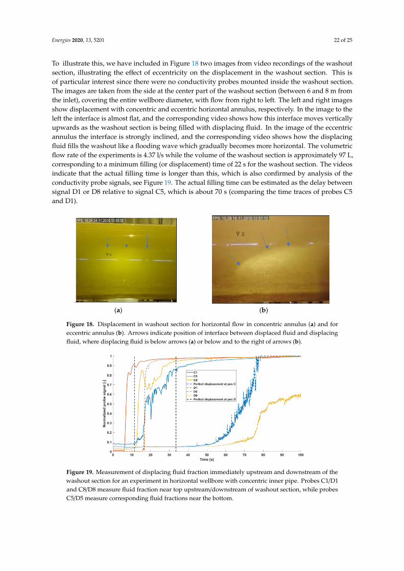
Energies 2020, 13, 5201 22 of 25

To illustrate this, we have included in Figure 18 two images from video recordings of the washoutsection, illustrating the effect of eccentricity on the displacement in the washout section. This isof particular interest since there were no conductivity probes mounted inside the washout section.The images are taken from the side at the center part of the washout section (between 6 and 8 m fromthe inlet), covering the entire wellbore diameter, with flow from right to left. The left and right imagesshow displacement with concentric and eccentric horizontal annulus, respectively. In the image to theleft the interface is almost flat, and the corresponding video shows how this interface moves verticallyupwards as the washout section is being filled with displacing fluid. In the image of the eccentricannulus the interface is strongly inclined, and the corresponding video shows how the displacingfluid fills the washout like a flooding wave which gradually becomes more horizontal. The volumetricflow rate of the experiments is 4.37 l/s while the volume of the washout section is approximately 97 L,corresponding to a minimum filling (or displacement) time of 22 s for the washout section. The videosindicate that the actual filling time is longer than this, which is also confirmed by analysis of theconductivity probe signals, see Figure 19. The actual filling time can be estimated as the delay betweensignal D1 or D8 relative to signal C5, which is about 70 s (comparing the time traces of probes C5and D1).


Figure 17. Effect of inner pipe rotation on displacement in inclined wellbore (60 degrees from vertical) with eccentric annulus (e = −0.42). Curves showing fraction of displacing fluid at station C (near inlet to washout section) without inner pipe rotation (experiment E1) and with inner pipe rotation (experiment F1). Azimuthal positions of probes (1, 5 and 8) are as shown in Figure 6.

Figure 17 also shows how the rotation breaks the symmetry in the response of probes 1 and 8 (these probes are located symmetrically with respect to the vertical diameter). Video cameras mounted along the test section provided additional qualitative information on the nature of the displacement. To illustrate this, we have included in Figure 18 two images from video recordings of the washout section, illustrating the effect of eccentricity on the displacement in the washout section. This is of particular interest since there were no conductivity probes mounted inside the washout section. The images are taken from the side at the center part of the washout section (between 6 and 8 m from the inlet), covering the entire wellbore diameter, with flow from right to left. The left and right images show displacement with concentric and eccentric horizontal annulus, respectively. In the image to the left the interface is almost flat, and the corresponding video shows how this interface moves vertically upwards as the washout section is being filled with displacing fluid. In the image of the eccentric annulus the interface is strongly inclined, and the corresponding video shows how the displacing fluid fills the washout like a flooding wave which gradually becomes more horizontal. The volumetric flow rate of the experiments is 4.37 l/s while the volume of the washout section is approximately 97 L, corresponding to a minimum filling (or displacement) time of 22 s for the washout section. The videos indicate that the actual filling time is longer than this, which is also confirmed by analysis of the conductivity probe signals, see Figure 19. The actual filling time can be estimated as the delay between signal D1 or D8 relative to signal C5, which is about 70 s (comparing the time traces of probes C5 and D1).

(a) (b)

Figure 18. Displacement in washout section for horizontal flow in concentric annulus (left panel) and for eccentric annulus (right panel). Arrows indicate position of interface between displaced fluid and

Loca

l fra

ctio

n of

dis

plac

ing

fluid

[-]

Figure 18. Displacement in washout section for horizontal flow in concentric annulus (a) and foreccentric annulus (b). Arrows indicate position of interface between displaced fluid and displacingfluid, where displacing fluid is below arrows (a) or below and to the right of arrows (b).


displacing fluid, where displacing fluid is below arrows (left image) or below and to the right of arrows (right image).

Figure 19. Measurement of displacing fluid fraction immediately upstream and downstream of the washout section for an experiment in horizontal wellbore with concentric inner pipe. Probes C1/D1 and C8/D8 measure fluid fraction near top upstream/downstream of washout section, while probes C5/D5 measure corresponding fluid fractions near the bottom.

5. Conclusions

A measurement system for liquid-liquid displacement experiments in concentric and eccentric annuli has been presented. Electrical conductance probes provide quantitative point measurements of the displacing fluid fraction at different axial and azimuthal positions along the wellbore, while video recordings provided supplementary qualitative information. The probes worked well, as demonstrated by overall consistency and repeatability of the signals. Albeit their individual response from point locations in the same vicinity from the wall, the combination of conductance probes gives an excellent measurement of the local average displacement process including mixing of miscible fluids. This electrical conductance technique has also been used successfully by other researchers [6–8] to generate displacement data and it should be accepted as a reliable method for measurement of displacement efficiency.

The video cameras used here covered the area between the arrays. Even with simple web-cameras as used in these experiments, video recordings can provide valuable supplement to and corroborate the conductance measurements. In the present experiments the analysis of the videos was difficult due to increasing opacity of the fluids, positioning of illumination and reflection of the illuminated light on the pipe wall. The recordings still provided qualitatively useful information. That was illustrated above by comparing the displacement pattern in the washout section for concentric and eccentric annuli, respectively.

The measured pressure gradient for sensor DP1 for horizontal annulus, agreed well with calculations both for concentric and eccentric annulus. A main motivation of the pressure measurements was to have a fluid quality check. As the calculations were based on viscometric measurements, the results demonstrated that the pressure measurements were consistent with the viscosimeter measurements.

Finally, the suitability of the device that was applied in the displacement studies presented by Renteria et al. [2], Tardy [4], Ytrehus et al. [16], Lund et al. [17,22] and Skadsem et al. [18] has been verified. Note that some of these studies have been used in development of displacement software.

Author Contributions: Conceptualization, J.D.Y. and A.S.; methodology, B.L. and A.T.; formal analysis, B.L.; investigation, A.T.; writing—original draft preparation, B.L.; writing—review and editing, B.L., J.D.Y., A.T. and A.S.; visualization, B.L. and A.T.; project administration, J.D.Y. All authors have read and agreed to the published version of the manuscript.

Figure 19. Measurement of displacing fluid fraction immediately upstream and downstream of thewashout section for an experiment in horizontal wellbore with concentric inner pipe. Probes C1/D1and C8/D8 measure fluid fraction near top upstream/downstream of washout section, while probesC5/D5 measure corresponding fluid fractions near the bottom.

Energies 2020, 13, 5201 23 of 25

5. Conclusions

A measurement system for liquid-liquid displacement experiments in concentric and eccentricannuli has been presented. Electrical conductance probes provide quantitative point measurements ofthe displacing fluid fraction at different axial and azimuthal positions along the wellbore, while videorecordings provided supplementary qualitative information. The probes worked well, as demonstratedby overall consistency and repeatability of the signals. Albeit their individual response from pointlocations in the same vicinity from the wall, the combination of conductance probes gives anexcellent measurement of the local average displacement process including mixing of misciblefluids. This electrical conductance technique has also been used successfully by other researchers [6–8]to generate displacement data and it should be accepted as a reliable method for measurement ofdisplacement efficiency.

The video cameras used here covered the area between the arrays. Even with simple web-camerasas used in these experiments, video recordings can provide valuable supplement to and corroboratethe conductance measurements. In the present experiments the analysis of the videos was difficult dueto increasing opacity of the fluids, positioning of illumination and reflection of the illuminated lighton the pipe wall. The recordings still provided qualitatively useful information. That was illustratedabove by comparing the displacement pattern in the washout section for concentric and eccentricannuli, respectively.

The measured pressure gradient for sensor DP1 for horizontal annulus, agreed well withcalculations both for concentric and eccentric annulus. A main motivation of the pressuremeasurements was to have a fluid quality check. As the calculations were based on viscometricmeasurements, the results demonstrated that the pressure measurements were consistent with theviscosimeter measurements.

Finally, the suitability of the device that was applied in the displacement studies presented byRenteria et al. [2], Tardy [4], Ytrehus et al. [16], Lund et al. [17,22] and Skadsem et al. [18] has beenverified. Note that some of these studies have been used in development of displacement software.

Author Contributions: Conceptualization, J.D.Y. and A.S.; methodology, B.L. and A.T.; formal analysis, B.L.;investigation, A.T.; writing—original draft preparation, B.L.; writing—review and editing, B.L., J.D.Y., A.T. andA.S.; visualization, B.L. and A.T.; project administration, J.D.Y. All authors have read and agreed to the publishedversion of the manuscript.

Funding: This research was funded through the Research Centre DrillWell, supported by the Research Council ofNorway, Aker BP, ConocoPhillips, Equinor and Wintershall. This publication was also financed by the researchgrant 294688, Optimized Wellbore Hydraulics.

Acknowledgments: The authors would like to thank the Research Council of Norway, Aker BP, ConocoPhillips,Statoil (now Equinor) and Wintershall, and for funding this work through the research centre DrillWell. The authorswould also like to thank MI-SWACO, Schlumberger for providing the chemicals used for the fluid design andthe technical support by Knud Richard Gyland. The authors also thanks Gunnar Lia Giil, Espen Johansen andBirgitte Ruud Kosberg for their assistance with the fluid design and control during their master program at NTNU,and PhD student Shreyansh Divyankar for assisting with displacement flow experiments. Last, but not least,the support with instrumentation and test preparation provided by our colleagues Terje Øyangen and Arne ErikRekkebo is highly appreciated.

Conflicts of Interest: The authors declare no conflict of interest.

Nomenclature

Symbol Description (Default) valueDi Inner diameter of annulus (outer diameter of inner pipe) 0.127 m (5”)Do Inner diameter of gauge outer pipe 0.1651 m (6.5”)Dwo Inner diameter of washout section 0.2794 m (11”)G Electrical conductance between electrodes of a probeGmax Conductance in high-conductivity fluidGmin Conductance in low-conductivity fluidK Gain factor of wave amplifier

Energies 2020, 13, 5201 24 of 25

Lp Length of probe electrodes (length into annulus) 5 mmLs Length of each pipe section 1.92 mLtot Total length of test section (ca) 10 mLwo1 Full bore length of washout section 1.66mLwo2 Length of increased diameter washout section 1.805 mQ Volumetric flow rateU Average flow velocity in regular section of annulus 0.5 m/sV Annular volume of the test sectionVo Measured voltage signal of a conductivity probeVo,max Measured voltage signal of a conductivity probe in high-conductivity fluidVo,min Measured voltage signal of a conductivity probe in low-conductivity fluidVoffset Offset voltage signal of a conductivity probeVr Relative voltage response.γ Fluid shear rate.γs Fluid characteristic shear rate∆ Center-center distance of electrodes 8 mmε Inner pipe eccentricity 0 and −0.42χ Displacement efficiencyδ Diameter of electrodes 3 mmλ Resistance per unit lengthθ Wellbore angle from verticalσ Electrical conductivity of fluidτ Fluid shear stressτs Fluid surplus stressτy Fluid yield stressψ Electrical resistivity of fluid

References

1. Daccord, G.; Guillot, D.; Nilsson, F. Mud removal. In Well Cementing, 2nd ed.; Nelson, E.B., Guillot, D., Eds.;Schlumberger: Sugarland, TX, USA, 2006; pp. 143–189.

2. Renteria, A.; Maleki, A.; Frigaard, I.A.; Lund, B.; Taghipour, A.; Ytrehus, J.D. Effects of irregularity ondisplacement flows in primary cementing of highly deviated wells. J. Pet. Sci. Eng. 2019, 172, 662–680.[CrossRef]

3. Maleki, A.; Frigaard, I.A. Primary cementing of oil and gas wells in turbulent and mixed regimes. J. Eng.Math. 2017, 107, 201–230. [CrossRef]

4. Tardy, P.M.J. A 3D model for annular displacements of wellbore completion fluids with casing movement.J. Pet. Sci. Eng. 2018, 162, 114–136. [CrossRef]

5. Wilson, M.A.; Sabins, F.L. A laboratory investigation of cementing horizontal wells (SPE16928). SPE Drill.Eng. 1988, 3, 275–280. [CrossRef]

6. Tehrani, A.; Ferguson, J.; Bittleston, S.H. Laminar Displacement in Annuli: A Combined Experimental andTheoretical Study. In Proceedings of the 67th Annual Technical Conference and Exhibition, Washington, DC,USA, 4–7 October 1992; Society of Petroleum Engineers: Richardson, TX, USA, 1992. SPE 24569.

7. Lockyear, C.F.; Ryan, D.F.; Gunningham, M.M. Cement channeling: How to predict and prevent (SPE 19865).SPE Drill. Eng. 1990, 5, 201–208. [CrossRef]

8. Deawwanich, T. Flow and Displacement of Viscoplastic Fluids in Eccentric Annuli. Ph.D. Thesis,The University of Adelaide, Adelaide, SA, Australia, March 2013.

9. Jakobsen, J.; Sterri, N.; Saasen, A.; Aas, B.; Kjøsnes, I.; Vigen, A. Displacements in Eccentric Annuli DuringPrimary Cementing in Deviated Wells. In Proceedings of the Production Operations Symposium, OklahomaCity, OK, USA, 7–9 April 1991; Society of Petroleum Engineers: Richardson, TX, USA, 1991. SPE 21686.

10. Vefring, E.H.; Bjørkevoll, K.S.; Hansen, S.A.; Sterri, N.; Sævareid, O.; Aas, B. Optimization of DisplacementEfficiency During Primary Cementing. In Proceedings of the Fifth Latin American and Caribbean PetroleumEngineering Conference and Exhibition, Rio de Janeiro, Brazil, 30 August–3 September 1997; Society ofPetroleum Engineers: Richardson, TX, USA, 1997. SPE 39009.

http://dx.doi.org/10.1016/j.petrol.2018.08.045

http://dx.doi.org/10.1007/s10665-017-9914-x


http://dx.doi.org/10.2118/16928-PA


Energies 2020, 13, 5201 25 of 25

11. Kimura, K.; Takase, K.; Griffith, J.E.; Gibson, R.A.; Porter, D.S.; Becker, T.E. Custom-Blending Foamed Cementfor Multiple Challenges. In Proceedings of the SPE/IADC Middle East Drilling Technology Conference,Abu Dhabi, UAE, 8–10 November 1999; Society of Petroleum Engineers: Richardson, TX, USA, 1999.SPE 57585.

12. Clark, C.R.; Carter, L.G. Mud displacement with cement slurries (SPE 4090). SPE J. 1973, 25, 775–783.13. Zuiderwijk, J.J.M. Mud displacement in primary cementation. In Proceedings of the SPE-European Spring

Meeting, Amsterdam, The Netherlands, 29–30 May 1974; Society of Petroleum Engineers: Richardson, TX,USA, 1974. SPE 4830.

14. Crook, R.J.; Keller, S.R.; Wilson, M.A. Deviated Wellbore Cementing: Part 2 Solutions. J. Pet. Tech. 1987, 39,961–966. [CrossRef]

15. Smith, D.K. Chapter 7. In Cementing; SPE Monograph Series; Society of Petroleum Engineers: Richardson,TX, USA, 1990; Volume 4.

16. Ytrehus, J.D.; Lund, B.; Taghipour, A.; Divyankar, S.; Saasen, S. Experimental investigation of wellborefluid displacement in concentric and eccentric annulus. In Proceedings of the 36th International Conferenceon Ocean, Offshore and Arctic Engineering, Trondheim, Norway, 25–30 June 2017; American Society ofMechanical Engineers: New York, NY, USA, 2017. OMAE-62028.

17. Lund, B.; Ytrehus, J.D.; Taghipour, A.; Divyankar, S.; Saasen, S. Fluid-fluid displacement for primarycementing in deviated washout sections. In Proceedings of the 37th International Conference on Ocean,Offshore and Arctic Engineering, Madrid, Spain, 17–22 June 2018; American Society of Mechanical Engineers:New York, NY, USA, 2018. OMAE-78707.

18. Skadsem, H.J.; Kragset, S.; Lund, B.; Ytrehus, J.D.; Taghipour, A. Annular displacement in a highly inclinedirregular wellbore: Experimental and three-dimensional numerical simulations. J. Pet. Sci. Eng. 2019, 172,998–1013. [CrossRef]

19. Saasen, A.; Lund, B.; Ytrehus, J.D. Theoretical Basis for Prediction of Drilling Fluid Removal in Annuli.In Proceedings of the 36th International Conference on Ocean, Offshore and Arctic Engineering, Trondheim,Norway, 25–30 June 2017; American Society of Mechanical Engineers: New York, NY, USA, 2017.OMAE-61030.

20. Kennelly, A.E. The Linear Resistance between Parallel Conducting Cylinders in a Medium of UniformConductivity. Proc. Am. Phil. Soc. 1909, 48, 142–165.

21. Saasen, A.; Ytrehus, J.D. Rheological Properties of Drilling Fluids–Use of Dimensionless Shear Rates inHerschel-Bulkley Models and Power-Law Models. Appl. Rheol. 2018, 28, 201854515.

22. Lund, B.; Ytrehus, J.D.; Taghipour, A.; Saasen, A. Displacement Efficiency In Eccentric Annuli. In Proceedingsof the 39th International Conference on Ocean, Offshore and Arctic Engineering, Virtual Conference,Fort Lauderdale, FL, USA, 3–7 August 2020; American Society of Mechanical Engineers: New York, NY,USA, 2020. OMAE-18707.

© 2020 by the authors. Licensee MDPI, Basel, Switzerland. This article is an open accessarticle distributed under the terms and conditions of the Creative Commons Attribution(CC BY) license (http://creativecommons.org/licenses/by/4.0/).



http://creativecommons.org/

http://creativecommons.org/licenses/by/4.0/.

Fluid Displacement in Irregular Annuli

Documents

Transcript of Fluid Displacement in Irregular Annuli