Flow in random porous media: mathematical formulation...

J. Fluid Me&. (1889), ~ 0 1 . 206, pp . 25-46 Printed in Great Britain

25

Flow in random porous media: mathematical formulation, variational principles,

and rigorous bounds

By JACOB RUBINSTEIN’? AND S. TORQUAT02 ‘Department of Mathematics, Stanford University, Stanford, CA 94305-2125, USA

a Department of Mechanical and Aerospace Engineering and Department of Chemical Engineering, Korth Carolina State University, Raleigh, NC 27695-7910, USA

(Received 27 June 1988 and in revised form 21 February 1989)

The problem of the slow viscous flow of a fluid through a random porous medium is considered. The macroscopic Darcy’s law, which defines the fluid permeability k, is first derived in an ensemble-average formulation using the method of homogenization. The fluid permeability is given explicitly in terms of a random boundary-value problem. General variational principles, different to ones suggested earlier, are then formulated in order to obtain rigorous upper and lower bounds on k. These variational principles are applied by evaluating them for four different types of admissible fields. Each bound is generally given in terms of various kinds of correlation functions which statistically characterize the microstructure of the medium. The upper and lower bounds are computed for flow interior and exterior to distributions of spheres.

1. Introduction

described by Darcy’s law (Scheidegger 1960 ; Dullien 1979) : The slow flow of an incompressible, viscous fluid through porous media is often

k P

u = - - vpo ,

where Uis the average velocity, V p , is the applied pressure gradient driving the flow, ,u is the fluid viscosity, and k is the fluid permeability which depends upon the random microstructure. There have been numerous attempts to rigorously derive (1 .1) . While the case of periodic geometry is now well understood (Tartar 1980; Keller 1980), little is known about flow in random geometries. Indeed, a rigorous derivation of (1.1) for flow through a highly dilute random array of fixed obstacles was given only recently by Rubinstein (1987). Simultaneously, many authors have attempted to compute k assuming that (1.1) is valid. The permeability, in general, depends upon an infinite set of correlation functions which statistically characterize the medium, however ; and except for specially prepared artificial media, this set of functions is never known. Again, in the periodic case, there are detailed results: both analytical (Hasimoto 1959) and numerical (Zick & Homsy 1982; Sangani & Acrivos 1982) ; whereas only dilute systems were studied for random microstructures using various effective-medium approximations whose validity is not yet clear (Brinkman 1947 ; Lundgren 1972 ; Childress 1972 ; Hinch 1977).

t Present address : Department of Mathematics, Technion-I.I.T. Haifa 32000, Israel.

26 J. Rubinstein and S. Torquato

Another approach concentrated on obtaining rigorous bounds for the permeability k . Bounds on effective parameters of random media are useful since : (i) they may be used to test the merits of a theory or computer-simulation experiment, (ii) as successively more microstructural information is included, the bounds (generally) become progressively narrower, and (iii) one of the bounds can typically provide a good estimate of the effective property, for a wide range of volume fractions, even when the reciprocal bound diverges from it (Torquato & Lado 1986). There are three basic steps involved in obtaining variational bounds on effective parameters of disordered media :

(1) defining the effective parameter in terms of some functional; (2) formulating an appropriate variational (extremum) principle for this

functional ; (3) and constructing trial fields which conform with the variational principle (i.e.

admissible fields). Prager (1961) and Weissberg & Prager (1970) were the first to derive upper bounds

on k. These bounds are referred to as ' three-point ' bounds since they involve up to three-point correlation function information. It should be noted that their derivations were formulated through physical reasoning and that the Prager and Weissberg-Prager variational principles (and their respective admissible fields) were different, Berryman & Milton (1985) subsequently, using a volume-average approach, corrected a normalization constraint in the Prager variational principle.

The main goal of this paper is to develop rigorous variational principles for flow in disordered porous media, and thus obtain rigorous upper and lower bounds on k. Both ensemble-average and volume-average formulations to the problem shall be presented. The ensemble-average approach is particularly useful in obtaining upper bounds on the permeability ; this avoids the difficulties encountered by Berryman & Milton (1985), Berryman (1986), and Caflisch & Rubinstein (1986) in handling boundary conditions for admissible fields in volume-average formulations. Torquato & Beasley (1987) recently reformulated the Weissberg-Prager variational upper bound on k in terms of ensemble averages. The Weissberg-Prager variational principle for the upper bound, however, is different to the corresponding principle derived in the present work.

In $2 we derive the Darcy formula (1 .1) for random porous media using the method of homogenization in an ensemble-average formulation. We then rewrite k in terms of an energy functional. In $ 3 we employ this functional to derive new variational principles for upper and lower bounds on the permeability. In $4 we apply these variational principles by explicitly evaluating the averages involved for four different types of admissible fields. The bounds so obtained are shown to depend upon various kinds of n-point correlation functions. In $5 we review a formalism to represent and compute the different types of correlation functions which arise in the bounds. The bounds are computed for media composed of random assemblages of spheres in $6. This is followed by a discussion in $ 7 .

2. Mathematical formulation 2.1. Derivation of the Darcy equation

There are several derivations of (1 .1) (Neumann 1977; Keller 1980; Tartar 1980; Whitaker 1986 among others). We give here another derivation based on an ensemble-averaging approach. This will turn out to be useful in obtaining variational principles for the permeability.

Flow in random porous media 27

The random medium is ti domain of space V(o) E R3 (where the realization a is taken from some probability space 0) which is partitioned into two regions : the void (pore) region Vl(o), through which fluid flows, of volume fraction (porosity) q51 and a solid-phase region V 2 ( w ) of volume fraction q52. Let a V ( w ) denote the surface between Vl and V2. The characteristic function of the pore region is defined by

1, rE.%(m)

0, rE"lrz(w) I ( r , o ) =

The fluid motion satisfies the Stokes equations:

pV2u = V p in Vl,

Veu = 0 in Vl,

u = O o n a Y . (2.4)

Here u and p are, respectively, the local velocity and pressure fields, and p is the fluid viscosity.

We assume that the random medium has a microscopic lengthscale 1 (e.g. the scale on which I ( r , w ) varies) which is small compared with a typical macroscopic lengthscale L (e.g. the scale on which the applied pressure gradient varies). Therefore, there is a small parameter e = 1/L associated with rapid fluctuations in the structure of Vl(o), and we assume that the velocity u and the pressure p depend on two scales : a slow scale x and a fast scale y = x / e , i.e.

p V 2 v ( x , y , 0 ) = V P ( X , Y , 0 ) in Y , " ( W ) , (2.5)

V . u ( x , y , o ) = 0 in V;(UJ), (2.6)

u ( x , y , w ) = 0 on aV. (2.7)

We shall derive the global (macroscopic) equations governing the flow using a two- scale expansion :

u ( x , y , 0) = e2uo(x,y, 0 ) +s3u,(x,y, w ) + ..., P(U>Y, w ) = P , ( X ) + ePl(u,Y, 0) + * * * ,

(2.8)

(2.9)

(2.10) 1 v = v,+-v,. e

The particular form of our expansion is motivated by the analysis of Sanchez- Palencia (1980) for periodic structures. Note that the first non-trivial term in the expansion for u is of O(e2) (in contrast to the expansion for the pressure). Physically, this is a consequence of the small pore size [O(e)] and the no-slip boundary condition. Substituting (2.8)-(2.10) into (2.5) and (2.6) and collecting powers of e yields the leading-order equations

p v ; ~ o ( x > Y , o ) = V , P l ( X ~ Y , ~ ) + V , P O ( ~ ) , (2.11)

V , % ( X , Y , 4 = 0, (2.12)

2

~ z ~ ~ o ~ x , y , ~ ) + v ~ ' u l ( x , y , w ) = 0. (2.13) FLM 208

28 J . Rubinstein and 8. Torquato

We now add the assumption that the medium is locally (i.e. on the y-scale) stationary. Ensemble averaging (2.13) gives

v,' u(x)+(v~'u1(x>y7w)) = O, (2.14)

where W ) = ( U O ) (4. (2.15)

Here (.) denotes an ensemble average. The second term of (2.14) is now shown to be zero. Let VR be a large sphere of radius R centred a t the origin. Then

where aV, is the surface of the large sphere. Using the boundary condition u1 = 0 on a V , we have

and letting R+ 03, we finally arrive at

v,. V ( x ) = 0. (2.16)

I n order to analyse (2.11) and (2.12), we introduce the stationary random functions w(y,w) = [wij] and 7t(y,w) = [nil which are the solutions of

Vi w = V, R- E in Vl(o), (2.17)

V,. w = 0 in Vl(o), w=O onaV(w).

(2.18)

(2.19)

Here E is the unit dyadic. We extend the quantities w a n d p in the solid region V 2 ( w ) to be zero. It is easy to verify that uo(x, y, o) and p l ( x , y, o) can be written as

1

P v,(x , Y, 0 ) = - - VPO(4 - W(Y 9 a), (2.20)

P,(x,Y,o) = VPo(x).4Y,o).

W ) = --(W(Y,o)).VPo(x).

Averaging (2.20), we obtain 1

P The permeability tensor is then defined by

k = (W(Y, w)>.

Therefore, (2.16) and (2.22) are rewritten as

k P

V ( x ) = --.Vpo(x),

(2.21)

(2.22)

(2.23)

(2.24)

v. U(x) = 0, (2.25)

which are the desired macroscopic equations : (2.24) being Darcy's law. Note that k is given explicitly in terms of the random boundary-value problem (2.17)-(2.19).


Henceforth, we assume the medium to be macroscopically isotropic, thus k = kE, where k = :( w: E) .

2.2. Energy characterization of the Permeability We now express the permeability k in terms of an energy functional.

Proposition 1 k = (Vw:VwI), (2.26)

where w is defined by (2.28)-(2.30).

vector equations ; the permeability is then redefined as Proof. For isotropic media, the auxiliary tensor equations (2.17)-(2.19) become

k = (Wae"), (2.27)

where e" is a unit vector and wCy, w ) solves

V2w = Vx-e" in V l ( w ) , (2.28)

V.w = 0 in Vl (w) , (2.29)

w = 0 on aVl(o). (2.30)

(Note that subscript y has been dropped from the gradient and Laplacian operators.) Multiplying (2.28) by w and averaging yields

k = (w-2) = (w.Vn)-(w.V~w}. (2.31)

We now integrate the right-hand side of (2.31) by parts and proceed aa in the derivation of (2.15). Boundary terms vanish identically because of the stationarity of w and n, and by (2.30). Thus, we obtain

k = -(TV.W)+(VW:VW).

The proposition follows from the incompressibility condition (2.29) and the extension of w into Vz.

3. Variational principles and bounds We consider deriving reciprocal variational principles for the boundary-value

problem described by (2.28)-(2.30). From these principles we then deduce upper and lower bounds on the permeability.

First we modify (2.28)-(2.30) slightly by introducing the functions q = yw and 5 = yn, where y is some positive constant. Then q and C solve

V2q(y, 0) = v a y , w ) -ye" in <(a), V.q(y,w) = 0 in <(a),

q@, 0) = 0 on aV(o),

k = - ( q - e ) = -(q-e"I).

and k satisfies 1 1

Y Y Proposition 2 -upper bound

Let A be the class of vector fields u defined by the set

A = {smooth, stationary functions u(y, w ) such that V x (V2u+ye") = 0 in "y;}. (3.5)

2-2

30

Then k is bounded from above by

J . Rubinstein and 8. Torquato

, V U E A . ( Vu : V U I )

Y 2 k <

Proof. From Proposition 1 it follows that

(4 : QqO Y2

k =

Let now U E A . Then there exists a function p"(y ,w) such that

v2u = Vp"- ye .̂ (3.7)

Writing u = q + g , pu = <+ h, we get

( VU: V U I ) = ( V q : V q I ) + ( V g : V g I ) + 2(Vq: V g I ) .

But from (3.7), i t follows that Vzg = V h and hence

Thus,

and Proposition 2 follows. The upper bound (3.6) that we derived here is different from the one proposed by

other investigators (Weissberg & Prager 1970 ; Berryman & Milton 1985 ; Berryman 1986). The normalization factor y2 in (3.6) is deterministic, in contrast to the normalization factor used in the aforementioned works, which is an integral over the random stress field. A formulation in which y is deterministic rather than stochastic is clearly preferred.

Proposition 3 -lower bound

( V q : V g I ) = ( V q : V g ) = - ( q * V h ) = ( h V - q ) = O .

(Vu: VUI) 2 ( V q : V q l )

Let B be the class of vector fields u defined by the set

smooth, stationary functions u(y, o) such that u = 0 017 3.v;

V - u = 0 B ={

in "y;, and (us&) = ( 4 - & I ) .

Then k is bounded from below by

Proof. Let U E B and define u = q + g . Then

(VU:VUI) = (Vq:VqI )+(Vg:QgI )+2(Vq: VgI ) . (3.10)

Integrating the last term by parts and using V - g = 0, we find

( V q : V g I ) = y(g.c?I) = y ( ( u . i I ) - ( q . i I ) ) = 0. (3.11)

Now eliminating y from (3.1) and (3.4), and applying Proposition 1, we obtain

(q.2I)2 ( V q : V q l ) . k = (3.12)

Equation (3.12) together with (3.10) and (3.11) proves Proposition 3, i.e. lower bound (3.9), which is new.


Remark. In certain instances it may be advantageous to use bounds that are cruder than (3.6) and (3.9), namely

(3.13)

(3.14)

The reason for this is that computation of ( V u : V u ) involves less detailed microstructural information (i.e. lower-order correlation functions) than the evaluation of ( V u : V u l ) .

Until now we have used an ensemble-average approach. An alternative derivation is possible by considering averages over a large but finite volume and then allowing the volume to expand to infinity. Let V be a large domain (in which we ultimately take the limit V + R3), a V be the surface of the domain, and consider

V2v = V p - ye" in Vl, (3.15)

W . v = O inVl , (3.16)

v = O onCIV, (3.17)

[~(vi,i+v,,()+psi,lni = 0 on CIV. (3.18)

Here vi,* = V V , ni is a unit normal, and 8, is the Kronecker delta. Next we define the volume average

(3.19) 1 g = - gdV. vsy

Then the permeability k is given by

(3.20) 1 k = lim -=.

v*w3 Y It is now possible to derive upper and lower bounds on k using volume averages

that are analogous to the ensemble-averaged bounds (3.6) and (3.9). We shall just give the volume-averaged lower bound since this is the only one we apply.

Proposition 4 (3.21)

(3.22)

The proof of lower bound (3.21) is similar to the proof of Proposition 3 and hence will not be presented here.

Our lower bounds (3.9) or (3.21) are different from the lower bounds of Rubinstein &, Keller (1987). In fact, the Rubinstein-Keller bounds are lower bounds on the inverse of the effective drag coefficient of the medium, while (3.9) or (3.21) are lower bounds on the geometrical factor k in Darcy's equation.

iz k 2 lim VUEB,,

B , = ( u ; W . u = O inVl, u = O oni3V, u . e I = v . S I ) .

v+Rs ut, j Ut , j I ' F -

4. Examples of trial fields and bounds In order to obtain explicit rigorous bounds on k for models of random porous

media, we must construct admissible trial fields which are contained in the sets (3.5), (3.8), or (3.22), substitute such trial fields into the respective variational bound, and

32 J . Rubinstein und 8. Torquuto

finally perform the necessary averaging. In what follows, we derive four different types of bounds.

4.1. Interfucial-surface upper bounds

We rederive an upper bound on k first obtained by Doi (1976) using Proposition 2. Our derivation is different to his, and in fact we show that his bound corresponds to a special choice of a trial field in the set A , (3.5), and not to a new variational principle as Doi stated. Specifically, we choose

u, (Y ,o ) = Y W(Y-x).[eI(x)-9(X)M(x)ldx, (4.1) s where y~ is the Stokeslet given by

and M ( x ) = IVI(X)l. (4.3)

The vector field < ( x ) defined on the interfacial surface i3-Y- is arbitrary. Accordingly, we refer to this construction as the ' interfacial-surface ' approach.

We now substitute (4.1) into (3.13) and compute the ensemble average (Vu,: Vu,). In so doing, we make use of the following two-point correlation functions:

Fvv(r) = ( I ( y ) I ( y + r ) ) , (4.4)

These functions are called void-void, surface-void, and surface-surface correlation functions, respectively. Such correlation functions and their generalizations (e.g. Fssv, Fsss, etc.) have been extensively studied by Torquato (1986b). We are free to choose c ( x ) subject to the constraint that (Vu, : Vu,) is finite. For simplicity we choose C ( X ) to be a constant vector 5,. Then (3.13) yields

The asymptotic behaviour of the correlation functions in (4.7) as Irl --t co is given by

Fss(r) Q2, %(r) - s91, Fvv(r) 91, (4.8)

where 4, = ( I @ ) ) is the expected volume fraction of the pore region V,, i.e. the porosity, and s = ( M ( y ) ) is the expected area of the interface 3-Y- per unit volume, i.e. the specific surface. Hence, the only choice of to for which the integral exists is

Therefore, substitution of (4.9) into (4.6) yields

(4.10)

For statistically isotropic media, the correlation functions depend only on the magnitude r = Irl and we have

(4.11)


The two-point upper bound (4.1 1) was first derived by Doi (1976). The derivation of (4.11) presented here, however, is new. The trial field (4.1) actually corresponds to a special choice of admissible fields in the set A . We further remark that Doi made the choice (4.9) after ‘optimizing’ over all possible to. However, as we have argued, any other choice for 5, provides the trivial bound k Q 00, so there is actually no room for optimization. Note that (4.1 1) is valid for any microgeometry that is statistically isotropic.

Phase-interchanged interfacial-surface bound .

Consider obtaining the phase-interchanged version of (4.1 l), i.e. consider deriving an interfacial-surface bound for flow occurring in phase 2 instead of phase 1. Before doing so, it is useful to rewrite (4.11) in a more general notation:

(4.12)

In (4.12), the superscript 1 emphasizes the fact that phase 1 is taken to be the void phase, i.e. the phase through which the fluid flows.

Let us now return to the problem of obtaining interfacial-surface bounds when phase 2 is taken to be the void or pore phase. The equation V x (V2u+yk) = 0 of (3.5) must now be satisfied in “tr,. The admissible field we must use is then the phase- interchanged counterpart of (4.1), i.e.

(4.13)

where J ( x , 0) = 1 -I(& 0) (4.14)

is the characteristic function of phase 2. Therefore, use of (3.13) gives the upper bound

where

(4.15)

is just the right-hand side of (4.12) and we have used the relations

Equation (4.15) is the analogue of a phase-interchanged bound for the rate constant of diffusion-controlled reactions (Torquato & Rubinstein 1988).

4.2. Void upper bounds Consider the following admissible field in the set A , (3.5) :

(4.16)

This is to be contrasted with the interfacial-surface trial field (4.1) with = (q4/s) 6, i.e.

(4.17)

34 J . Rubinstein and S. Torquato

Recall that (4.17) leads to the two-point bound (4.10) or, equivalently, (4.11). Consider the terms within the brackets of (4.16) and (4.17). Although the first terms are the same to within a factor of $ 2 , the second term of (4.16), unlike (4.17), does not involve interfacial information. As we shall discuss in $6, the surface integration of (4.17) is required in order to obtain the correct dilute-limit result for spheres. Substitution of (4.16) into (3.13) yields for general statistically isotropic media :

n Pm

(4.18)

The two-point void bound (4.18) is equal to an upper bound obtained by Berryman & Milton (1985) using a different approach. First, Berryman & Milton use a different variational principle in which the normalization factor y is a stochastic rather than a deterministic quantity as in the present work. Second, they use a volume-average formulation for the variational upper bound. Unfortunately, it is difficult to construct admissible fields that satisfy the required boundary conditions in the volume-average approach. Nonetheless, our derivation demonstrates that (4.18) is a rigorous upper bound on k .

Phase-interchanged void bound Consider obtaining the phase-interchanged counterpart of (4.18), i.e. consider flow

occurring in phase 2 instead of phase 1. The admissible field for the phase- interchanged principle (3.13) is then

and hence we find the upper bound

n Pm

(4.19)

(4.20)

where we have employed the relation

F:: - 4; = FkV - &. Finally, we point out that the void bounds given here are the analogues of bounds Torquato & Rubinstein (1988) derived on the rate of diffusion-controlled reactions.

4.3. Multiple-Scattering Upper Bounds If the medium is composed of a distribution of inclusions and flow is considered to occur in the region exterior to the inclusions (phase l) , we can construct trial fields which are based on the solutions for scattering from a single inclusion, pairs of inclusions, etc. Accordingly, we refer to bounds so obtained as multiple-scattering bounds. For simplicity we shall consider here the case of a distribution of identical spheres with radius a. The single-sphere scattering function S(x, y ) is given by

S ( x , y ) = [1 + W A I W ( X , Y ) . (4.21)

Note that the velocity field outside a single sphere moving with velocity U in an otherwise viscous, quiescent fluid is S - U. We also define

0, r < a 1 , r > a

(4.22)


to be the characteristic function of the exterior of a single sphere. Then we can construct the following single-scatterer trial field :

(4.23)

where ri denotes the position of the ith sphere and a is a parameter to be optimized. It turns out that the only choice for which the energy (Vu,: Vu, I ) is finite is a = l /p, where p is the number density of spheres. Trial fields of this type have been employed in the problems of conduction in composite media (Torquato 1986a), viscous flow in porous materials (Torquato & Beasley 1987), and in diffusion-controlled reactions in heterogeneous media (Rubinstein & Torquato 1988). Next we define the tensor z through

z = V ( S . i ) + V ( S . l ) T , (4.24)

where the second term of the right-hand side of (4.24) is the transpose of the first term.

Substitution of (4.23) into (3.13) then yields the two-point upper bound

where (4.26)

is the total correlation function, pn(r l , . .., r,) is the probability density associated with finding n spheres with configuration rl , ..., r,, as defined by (5.1), y , = y - r i , y1 = JyJ, and rif = rj -r i . For statistically homogeneous media, pl(r l ) = p. Note that the integrals of (4.25) are absolutely convergent; the second one is convergent since h(r) tends to zero much more rapidly than r-3 as r+ co. Since the first integral in (4.25) can be computed explicitly, we have

(4.27)

The first term of (4.27) is the exact Stokes dilute-limit result. If we substitute (4.23) in (3.6), we obtain the following three-point upper bound:

and G,(x; rQ) (n = 1 +q) is the point/q-particle distribution function (Torquato 1986a) which gives the correlation associated with finding a point with position x in Vl and q spheres with configuration rQ = {rl, . . . , r,}. It is clear that G,(x; 6) = 0 if Ix-rJ < a, i = 1, ..., q. For stationary media, the G, depend only upon relative displacements, i.e. G,(x; ra) = G n ( x - r l , ..., x-rQ) . The asymptotic behaviour of Q3

for large separation of the points ensures the absolute convergence of the second integral of (4.28). An explicit representation of the G, is given in $ 5 .

It must be noted that the multiple-scattering upper bound on k derived by

36 J . Rubinstein. and S. Torquuto

Torquato & Beasley (1987) using a probabilistic formulation of the Weissberg-Prager (1970) variational principle is very similar to (4.28). It was found that

SC,lv1)r(y,):r(Y,)dr,t &,(Yl,Y,)~(Yl):~(r2)dr,dr, kd ss A2 > (4.30)

where A is a multidimensional integral over the trial stress field acting over the random interface As noted earlier, the advantage of the present formulation is that the normalization factor is deterministic and does not have to be explicitly evaluated.

4.4, Security-spheres lower bound

We shall employ the security-spheres method to construct trial fields in the set B, (cf. (3.22)). This method goes back to Keller, Rubenfeld & Molyneux (1967) who used i t to estimate the effective viscosity of suspensions. It has been used recently by Rubinstein & Keller (1987) to derive upper bounds on the effective drag coefficient, and by Rubinstein & Torquato (1988) to study the reaction rate constant in diffusion-controlled reactions.

Consider a distribution of N identical spheres with radius u. Let the distance between the ith sphere and its nearest neighbour be denoted by 2bi. For every sphere d we consider the domain defined by itself and a concentric ‘security’ sphere of radius bi. In that domain we solve

V2ui = Vpi in a < Ix-rJ < b,, (4.31)

V . u i = 0 in a < Ix-rJ < b,, (4.32)

ui = 0 on Ix-ril = a, (4.33)

ui = U on Ix-rJ = bi, (4.34)

where U is an arbitrary constant vector. Now a trial field w(x) in B, (cf. (3.22)) is defined to be equal to ui for a < Ix-rJ < b, and equal to U when x is outside all the security spheres. Without loss of generality, we choose 6 (and U) in the positive x-direction. The incompressibility of the flow implies

u,e^dx = $xb3U. (4.35) s a<Ix-rtl<bt

Thus the numerator in (3.21) is identically V. The only contributions to the rate of energy dissipation are from the security spheres. I n the kth (Happel & Brenner 1983):

~ ~ ~ u ~ , ~ d x = 6 n a V f s a < /x-rk/ < bk

where 9a 5a3 9a5

f ( a ) = (1-a5) ( 4 2 4 1 - - + - - - + ~ 6

Hence we obtain from (3.21)

where a, = a /bk

security shell we find

(4.36)

(4.37)

(4.38)

(4.39)


and p is the sphere number density. Scaling k with the Stokes permeability ks = (6nap)-l, and using the law of large numbers we have

(4.40)

Here H ( b ) is the probability density of spheres with nearest neighbour at distance 2b. The bound (4.40) coincides with the Rubinstein-Keller bound on the effective drag coefficient. This is, however, merely a coincidence and results from our particular choice of u' ((4.31)-(4.34)), and the identity (4.35). Other trial fields (e.g. in the spirit of Torquato & Rubinstein 1989) would yield improved bounds. We believe, though, that before searching for better trial fields, one should first calculate H(b) for realistic geometries. We are currently working on that problem.

5. Statistical characterization of the microstructure In order to compute the aforementioned bound, one must be able to determine the

correlation functions that are involved. Torquato (1986b) has recently developed a general framework from which one may derive and calculate all of the various kinds of correlation functions that have arisen in expressions for transport, mechanical, and electromagnetic properties of two-phase disordered media composed of random distributions of inclusions. This is accomplished by introducing a general n-point distribution function H , for such a medium.

Consider a random distribution of N identical spheres of radius a with positions rN E { r l , .. . , r,}. Let PN(rN) be the probability density function associated with the event of finding particles 1, . . . , N with configuration r N , respectively. Then

n -- N ! k N ( r N ) drn+l . . . dr, p n ( r I - (N-n) !

is the probability density function associated with finding any subset of n( < N ) particles with configuration r". Let phase 1 and phase 2 be the space exterior and interior to the spheres, respectively. Among other quantities, Torquato (1986 b ) defines and obtains a series representation of the following general n-point distribution for such a system of particles:

where

; x P - ~ ; rq) = Correlation associated with finding a point with position x, on i3.v; ..., and a point with position x, on ac and a point with position x,+~ in "y;, ..., and a point with position x p in Yl, and of finding any q spheres with configuration r"l, where XP-m (x,+~, ..., x,} and n = p + q m

= (- l)iH',Z)(xm ; xP-, ; rg), (5 .2) i-0


P m(P) = 1- n [l-m(yij;Ri)],

i-1

(5.7)

and yij = Ixi - r J . Note that the H , are quite general and contain, as special cases, all of the aforementioned statistical quantities [e.g. s = H,(x , ; 0 ; a), = H , ( @ ; x , ;

O;rn), S,(xn) = H , ( @ ; x " ; f a ) , and Gn(x , ; rq ) = H , ( @ ; x , ; r q ) , whcrc 0 denotes the empty set] and their generalizations [e.g. Fssv(xl ,xz ,x3) = H3(x1,x2 ; x,; @), ctc.]. Here S,(xn) is the probability of finding n points in phase 1 (e.g. AS, = 9, and S, = Fvv) : quantities first studied by Torquato & Stell (1982). The derivatives of (5.3) serve to bring out information about the interface. It is important to emphasize that the H , are given in terms of the probability density functions that characterize the configuration of the inclusions, i.e. the p,. Given the p n for the ensemble, one may now compute the H , using (5.2)-(5.7). Finally, we remark that Torquato (19863) actually studied n,-point distribution functions that characterize media that are more general than the class of models considered here.

Models of random media composed of identical spheres are not as restrictive as one might initially surmise. For example, the spheres can be distributed with an arbitrary degree of impenetrability A. One can construct. models in which the impenetrability parameter h varies continuously between zero (in the case where the sphere centres are randomly centred, i.e. 'fully penetrable ' spheres) and unity (in the instance of totally impenetrable spheres). The topological property of 'connectedness' of the sphere phase is clearly dependent upon the degree of impenetrability A, e.g. for fully penetrable spheres ( A = 0) and an equilibrium distribution of totally impenetrable spheres ( A = l ) , the sphere phase percolates (i.e. a sample-spanning cluster appears) a t a sphere volume fraction q52 of about 0.3 (Haan & Zwanzig 1977) and 0.64 (Berryman 1983), respectively: the latter value corresponding to the random-close-packing limit. (It is noteworthy that a fully penetrable-sphere system is bicontinuous for 0.3 < $2 < 0.97, where $, x 0.97 corresponds to the point a t which the space exterior to the spheres first become disconnected (Elam, Kerstein & Rehr 1984).) Therefore, interpenetrable-sphere models can be used to study fluid transport in both unconsolidated media (e.g. beds of discrete particles) by setting h = 1 and consolidated media (e.g. sandstones, sintered materials, etc.) by considering h < 1. For h < 1, fluid can flow in the connected region exterior or interior to the sphere phase (e.g. for h = 0, fluid can flow in the space exterior to the spheres for 0 < $, < 0.97 or inside the sphere phase for 0.3 Q $2 < 1). Note that information about the impenetrability of the spheres in equation (5 .2 ) for the H , enters through the p n defined by (5.1).

An example of an interpenetrable-sphere distribution is the permeable-sphere (PS) model (Salacuse & Stell 1982). I n the PS model, the spheres are assumed to be (structurally) non-interacting when non-intersecting, with a probability of inter- section given by a radial distribution function g(r ) = 1 -h[g(r ) = p, ( r ) /p2 ] , independent of the interparticle separation distance r when r < 2a. Another example of an interpenetrable-sphere distribution is the penetrable-concentric-shell (PCS) model (Torquato 1984). In the PCS model, spherical particles of radius a are randomly distributed subject to the condition of a mutually impenetrable core region of radius ha, 0 < h < 1. Each sphere may be thought of as being composed of an

0), J'sv(xl3~2) = HZ(x1; x2 ; fa), F s s ( ~ 1 , ~ 2 ) = H,(x , ,x , ; 0 ; 0 ) 3 pn(r") = H n ( 0 ;


FIGURE 1. A computer-generated realization of a distribution of disks of radius a = tu (shaded region) in the PCS model (Torquato 1984). The disks have an impenetrable core of diameter hu indicated by the smaller, black circular region. Here A = 0.5 and q52 = 0.3.

impenetrable core of radius ha, encompassed by a perfectly penetrable concentric shell of thickness (1 - A ) a (cf. figure 1). I n the PS model, two particle centres may lie arbitrarily close to one another such that the probability of overlap is 1 - h ; in the PCS model no two particle centres may lie closer than the distance 2ah. Moreover, although the PS model assumes a condition of thermal equilibrium, along with the constraints explicitly stated above, the PCS model is not restricted to an equilibrium ensemble of particles. The impenetrability condition of the internal hard core of radius Aa does not uniquely determine the distribution in the latter model. Hence, in the PCS model, one may assume an equilibrium or some non-equilibrium distribution, such as random sequential addition (Widom 1966). I n the following section, we shall report, among other results, bounds on the permeability for distributions of spheres in both the PS and PCS models.

6. Evaluation of bounds 6.1 Evaluation of the interfacial-surface upper bounds for distributions of spheres

Flow around spheres Employing the series representation o€ the general n-point distribution function

H , , (5.2)-(5.7), Torquato & Beasley (1987) computed the interfacial-surface upper bound (4.12) for flow around identical spheres of radius a in both the PS and PCS models :

k(1)

- < 1 -&42 + O(&), (6.1) ks

where k, = 2a2/9$, (6.2)

is the exact Stokes dilute-limit result, and where K ==+?A

2 8


is the scaled second-order coefficient in the PS model. K , accounts for interactions between pairs of spheres. As the impenetrability parameter h increases, the coefficient K, increases (since the surface area of the obstacles increases) ; thus the upper bound on k(l) decreases with increasing h for fixed but small $z. Torquato & Beasley computed K , numerically in the PCS model and found that for h = 0.2, 0.4, 0.6, and 0.8, K , = 1.88, 1.96, 2.30, and 2.36, respectively. Note that for the extreme limits h = 0 and h = 1, the PS and PCS models are the same for any sphere concentration, assuming an equilibrium distribution. Moreover, although an equilibrium ensemble of spheres in the PCS model is generally different to the corresponding model in the non-equilibrium random-sequential ensemble (Widom 1966), they are the same up to the level of the third virial coefficient and hence the Torquato-Beasley results for the PCS model apply as well to this non-equilibrium distribution.

It is of interest to compare the low-density bound (6.1) to the low-density expansion of k( l ) obtained from effective-medium approximations (Brinkman 1947 ; Lundgren 1972 ; Childress 1972 ; Hinch 1977) for totally impenetrable spheres :

The expansion (6.4) predicts an O($%) correction to the Stokes-law limit as opposed to an O(q5,) correction from the bound (6.1). The non-analytic dependence on q5z (cf. (6.4)) is a direct consequence of hydrodynamic screening effects. Clearly, for dilute conditions, the q5: term is the dominant one. It is difficult to construct trial fields which incorporate screening and simultaneously satisfy the conditions of the set A , (3.5). On the other hand, it is difficult to treat flow around overlapping spheres using effective-medium approximations. Moreover, a t small porosities, effective-medium theories are not accurate and hence, for high solid volume fractions, bounds provide the only rigorous means of estimating the permeability.

Upper bound (4.12) has been computed to all orders in $, for flow around fully penetrable spheres (cf. figure 2) by Doi (1976) and totally impenetrable spheres by Torquato (19863). We refer to the former as the ‘Swiss-cheese’ model, i.e. the case in which transport occurs exterior to fully penetrable spheres. For subsequent discussion, we summarize these results in figure 3. It is noteworthy that the upper bound for A = 1 given in the figure is the closest that a rigorous bound has come to the empirical Kozeny-Carman relation.

Flow inside spheres Here we shall compute the phase-interchanged interfacial-surface bound (4.15) for

flow interior to fully penetrable spheres ( A = 0) of radius a, i.e. the void phase (phase 2) is the sphere phase. We term this the ‘inverted Swiss-cheese’ model. For fully penetrable spheres, the n-particle probability density pn is simply equal to p” and hence the two-point correlation functions that arise in (4.15) can be obtained analytically from (5.2)-(5.7). For example, the number density of spheres p is related to (the volume fraction of the solid region) by the simple expression $1 = exp ( - T ) , where 7 = 3 a 3 p is a reduced density. (This is to be contrasted with the case of totally impenetrable spheres for which $1 = 1-7.) Furthermore, for h = 0, the specific surface s = 3174Ja (whereas for h = 1, s = 3$, /a) . As noted earlier, for $, < 0.03, the solid region is disconnected and the obstacles are the oddly shaped ‘holes’ between the spheres (cf. figure 4). At q51 x 0.03, the space exterior to the spheres percolates. The permeability is expected to decrease as is increased. At


FIGURE 2. A computer-generated realization of fully penetrable (i.e. randomly centred) disks a t q52 x 0.5. Transport occurs outside the particles. We term this the ‘Swiss-cheese’ model.

0.01 I I I I I

0 0.2 0.4 0.6 0.8 1 $2

FIGURE 3. Upper bounds on the scaled permeability k ( l ) / k , versus the solid volume fraction q5z( k, = 2az/9q5,) : -, two-point interfacial-surface bound (4.12) for totally impenetrable spheres ( A = 1 ) computed by Torquato (1986b); ---, two-point interfacial-surface bound (4.12) for the Swiss-cheese model computed by Doi (1976) ; . . . . , three-point multiple-scattering bound (6.9) for the Swiss-cheese model.


I ‘

I ‘ 4

t V

FIGURE 4. Distribution of fully penetrable disks at a very high volume fraction of disks. The solid region (black area) is composed of the ‘holes ’ between the disks. Flow takes place in the disk region (white area). This is termed the ‘inverted Swiss-cheese’ model.

dl x 0.7, the sphere phase (the region in which transport takes place) ceases to percolate ; and hence, a t this transition, the permeability must vanish.

It is of interest to study the behaviour of (4.15) for the inverted Swiss-cheese model in the limit $, < 1. Denoting the right-hand side of (4.15) by k z ) and carrying out the asymptotic expansion, we find

Since the holes are not spherically symmetric, result (6.5) cannot be expected to be the exact dilute limit. This is in contrast to the other extreme case $z < 1 for the Swiss-cheese model (flow around fully penetrable spheres) where bound (4.11) captures the Stokes dilute limit. We do conjecture, however, that the dilute limit of k@) is of the form caz(lnq51)-2q51-1, with c d $.

In figure 5 we plot the scaled permeability k ( 2 ) / k , (where k, = 4a2/9(ln q51)2q51) as a function of the volume fraction of the solid region. Note that the spike which appears in the figure for small q51 has no physical significance ; it is the result of our use of the scaling factor k,.

We compute (4.15) for the case h = 0 to all orders in

6.2. Evaluation of the void upper bounds for distributions of spheres Flow around spheres

Consider calculating the void upper bound (4.18) for flow around a dilute array of equisized spheres. Using the low-density expansion of F,, for a distribution of identical spheres of radius a (Torquato & Stell 1982), we find

k(’) d a 2 [ z + O ( l ) ] . W2

Unlike the interfacial-surface upper bound (cf. (6.1)), the void upper bound does not give the exact Stokes result (6.2) in the limit q5z -+ 1.


n Inverted swiss-cheese model

I 0.2 0.4

61 6

FIQURE 5. The scaled permeability k ( 2 ) / k , (where k, = 4~~/9(lng5,)~g5,) as & function of the solid volume fraction for the inverted Swiss-cheese model in which the spheres have radiue a.

Flow inside spheres Suppose we now consider evaluating the phase-interchanged void bound (4.20) for

the inverted Swiss-cheese model (cf. figure 5). Then for small concentration of the trap phase < l), bound (4.20) yields

which is not as sharp as the interfacial-surface counterpart (6.5).

6.3. Evaluation of the multiple-scattering upper bounds for distributions af spheres Here we calculate the multiple-scattering upper bounds (4.27) and (4.28) for flow around spheres. First consider the exact evaluation of the two- and three-point upper bounds to all orders in $2 for the case of fully penetrable spheres ( A = 01, i.e. the Swiss-cheese model. For such distribution, h(r) = 0 for all r , and the two-point upper bound (4.27) simply gives

Comparing (6.8) to the interfacial-surface upper bound (4.12) for h = 0 reveals that the latter is the sharper of the two through all orders in q52, For this model, the G,, described by (5.2), are trivial (Torquato 1986a b ) , and the three-point bound (4.28) yields

which is clearly a better upper bound than (6.8). Therefore, incorporation of additional statistical information in multiple-scattering-type bounds leads to progressively sharper bounds. In figure 3, we include lower bound (6.9). Although


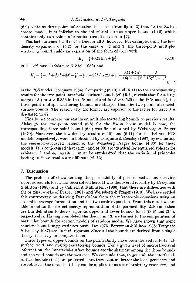
(6.9) contains three-point information, i t is seen (from figure 3) that for the Swiss- cheese model, it is inferior to the interfacial-surface upper bound (4.12) which contains only two-point information (see discussion in $ 7).

This last statement will not be true for all A, however. For example, using the low- e- density expansion of (5.2) for the cases n = 2 and 3, the three-point multi]

scattering bound yields an expansion of the form of (6.1) with

K , = i+h(31n3++3 (6.

in the PS model (Salacusc & Stcll 1982) and

0)

h(l+7h) h 16(2h+1)2+16(2h+1)4

K 2 2 = 3 - h 6 + ~ h 4 + ~ h 2 - ~ A +2(1+ 3h2) In (2h + 1)- (6.11)

in the PCS model (Torquato 1984). Comparing (6.10) and (6.11) to the corresponding results for the two-point interfacial-surface bounds (cf. $6.l), reveals that for a large range of h (for h > 0.356 in the PS model and for h > 0.520 in the PCS model), the three-point multiple-scattering bounds are sharper than the two-point interfacial- surface bounds. The reason why the former are superior to the latter for large h is discussed in $7.

Finally, we compare our results on multiple-scattering bounds to previous results. Although the two-point bound (6.8) for the Swiss-cheese model is new, the corresponding three-point bound (6.9) was first obtained by Weissberg & Prager (1970). Moreover, the low-density results (6.10) and (6.11) for the PS and PCS models, respectively, were first obtained by Torquato & Beasley (1987) by evaluating the ensemble-averaged version of the Weissberg-Prager bound (4.30) for these models. It is conjectured that (4.29) and (4.30) are identical for equisized spheres for arbitrary h and Again, it must be emphasized that the variational principles leading to these results are different (cf. $3).

7. Discussion The problem of characterizing the permeability of porous media, and deriving

rigorous bounds for it, has been solved here. It was discovered recently by Berryman & Milton (1985) and by Caflisch & Rubinstein (1986) that there are difficulties with the original works of Prager (1961) and Weissberg & Prager (1970). We have settled this controversy by deriving Darcy’s law from the microscopic equations using an ensemble-average formulation and the two-scale expansion. From this result we are able to obtain the correct energy representation of the permeability (2.26) and then use this definition to derive rigorous upper and lower bounds for it ((3.6) and (3.9), respectively). Having completed the theory in $3, we turned to the computation of particular bounds for certain models of random media. We have shown that some heuristic bounds suggested previously (Doi 1976 ; Berryman & Milton 1985 ; Torquato & Beasley 1987) are, in fact, rigorous. Since all the bounds are derived from a single theory, i t is easy to compare them.

Three types of upper bounds on the permeability have been derived : interfacial- surface, void, and multiple-scattering bounds. For a given level of microstructural information, the interfacial-surface bounds are the sharpest among the three bounds and the void bounds are the weakest. We conclude that, in general, the interfacial- surface bounds ($4.1) are preferred since they capture better the local geometry and are robust in thc sense that they can be applied to media of arbitrary geometry, and


hence to real materials. On the other hand, the multiple-scattering bounds developed in 54.3 are limited to flow around distributions of inclusions. The advantage of these bounds, however, is that one can systematically upgrade them by including sophisticated multiple-scattering solutions.

It is interesting to observe that for dispersions of non-overlapping spheres ( A = l) , the interfacial-surface trial field (4.1) and the multiple-scattering (4.23) are very similar. This is the result of our choice for 6 in (4.9) and the mean-value theorem for biharmonic functions

As in the analysis of the analogous bounds for the rate of diffusion-controlled reactions (Rubinstein & Torquato 1988), one can use result (7.1) to explain why the two-point interfacial-surface bound is weaker than the three-point multiple- scattering bound for sphere distributions characterized by a large degree of impenetrability h and why the converse is true for small A.

We also derive a new lower bound on the fluid permeability. Lower bounds are much harder to obtain than upper bounds. In fact, it was conjectured in the past that it is not possible to write such bounds at all. Using the security-spheres method, we derived the simple formula (4.40) in terms of the nearest-neighbour distribution function. We are currently in the process of evaluating this function for several models. Another direction we are taking is to find interfacial-surface bounds which use three-point (or more) correlation functions.

Finally, we remark that while approximate theories exist to predict k, bounding methods provide the only rigorous means of obtaining reasonable estimates for effective parameters of real media for arbitrary porosities, and there lies their practical importance.

S. Torquato gratefully acknowledges the support of the Office of Basic Energy Sciences, US Department of Energy, under Grant No. DE-FG05-86ERl3482. J. Rubinstein was supported by the National Science Foundation and the Office of Naval Research.

REFERENCES

BERRYMAN, J. G. 1983 Random close packing of hard spheres and disks. Phys. Rev. A 27, 1053. BERRYMAN, J. G. 1986 Variational bounds on Darcy’s constant. In Homogenization and Effective

Moduli of Materials. IMA Volumes in Mathematics and Its Application, vol. 1, Springer. BERRYMAN, J. G. & MILTON, G. W. 1985 Normalization constraint for variational bounds on fluid

permeability. J . Chem. Phys. 83, 754. BRINKMAN, H . C. 1947 A calculation of the viscous force exerted by a flowing fluid on a dense

swarm of particles. Appl. Sci. Res. A l , 27. CAFLISCH, R. E. & RUBINSTEIN, J. 1986 Lectures on the Mathematical Theory of Multiphuse Flow.

Courant Institute Notes Series, Kew York University. CHILDRESS, S. 1972 Viscous flow past a random array of spheres. J . Chem. Phys. 56, 2527. DOI, M. 1976 A new variational approach to the diffusion and flow problem in porous media.

DULLTEN, F. A. L. 1979 Porous Media. Academic. ELAM, W. T., KERSTEIN, A. R. & REHR, J. J. 1984 Critical properties of the void percolation

problem for spheres. Phys. Rev. Lett. 52 , 1516. HAAN, S. W. & ZWANZIG, R. 1977 Series expansions in a continuum percolation problem. J. Phys.

A 10, 1547.

J . Phys. Soc. Japan 40, 567.

46

HAPPEL, J. & BRENNER, H. 1983 Low Reynolds Number Hydrodynamics. Nijhoff. HASIMOTO, H. 1959 On the periodic fundamental solutions of the Stokes equations and their

application to viscous flow past a cubic array of spheres. .I. Pluid Mech. 5, 317. HINCH, E. J. 1977 An averaged-equation approach to particle interactions in a fluid suspension.

J . Fluid Mech. 83, 695. KELLER, <J. B. 1980 Darcy’s law for flow in porous media and the two-scale method. Tn Nonlineur

P.D.E. in Engineering and Applied Sciences (ed. R. L. Sternberg, A. J. Kalinowski & J. S. Papadakis). Marcel Dekker.

KELLER, J . B., RUBENFELD, L. & MOLYNEUX, J. 1967 Extremum principles for slow viscous flows with applications to suspensions. J . Fluid Mech. 30, 97.

LUNDGREN, T. S. 1972 Slow flow through stationary random beds and suspension of spheres. J . Fluid Mech. 51, 273.

NEUMAN, S. P. 1977 Theoretical derivation of Darcy’s law. A&. Mech. 25, 153. PRAGER, S. 1961 Viscous flow through porous media. Phys. Fluids 4, 1477. RUBINSTEIN, J . 1987 Hydrodynamic screening in random media. Tn Hydrodynamic Hrhavior

and Interacting ParticZe Systems. TMA Volumes in Mathematics and Tt.s Application. vol. 9 (ed. G. Papanicolao) Springer.

J . Rubinstsin and S. Torquato

RUBINSTEIN, J . 8: KELLER, J. B. 1987 Lower bounds on permeability. Phys. Fluids 30, 2919. RUBINSTEIN, J. & TORQUATO, S. 1988 Diffusion-controlled reactions : mathematical formulation,

variational principle, and rigorous bounds. J . Chem. Phys. 88, 6372. SALACUSE, J. J. & STELL, G. 1982 Polydisperse systems : statistical thermodynamics with

applications to several models including hard and permeable spheres. J . Chem. Phys. 77, 3714. SANCHEZ-PALENCIA, E. 1980 Nonhomogeneous media and vibration theory. Lectures Notes in

Physics, vol. 127. Springer. SANGANI, A. & ACRIVOS, A. 1982 Slow flow through a cubic array of spheres. Intl , I . Multiphase

Flow 8, 343. SCHEIDEGGEK, A. E. 1960 The Physics of Flow through Porous Media. Macmillan. TARTAR, L. 1980 Nonhomogeneous Media and Vibration Theory, Appendix 2. Lecture Notes in

Physics, vol. 127. Springer. TORQUATO, S. 1984 Bulk properties of two-phase disordered media: I. Cluster expansion for the

effective dielectric constant of dispersions of penetrable spheres. J . Chem. Phys. 81, 5079. TORQUATO, S. 1986a Bulk properties of two-phase disordered media: 111. New bounds on the

effective conductivity of dispersions of penetrable spheres. J . Chem. Phys. 84, 6345. TORQUATO, 6. 1986 b Microstructure characterization and bulk properties of disordered two-phase

media. J . Statist. Phys. 45, 843. TORQUATO, S. & BEASLEY, J. D. 1987 Bounds on the permeability of a random array of partially

penetrable spheres. Phys. Fluids 30, 633. TORQUATO, S. & LADO, F. 1986 Effective properties of two-phase disordered composite media: 11.

Evaluation of bounds on the conductivity and bulk modulus of dispersions of impenetrable spheres. Phys. Rev. B 33, 6428.

TORQUATO, S. & RUBINSTEIN, J. 1988 Diffusion-controlled reactions. 11. Further bounds on the rate constant. J . Chem. Phys. 90, 1644.

TORQUATO, S. & STELL, G. 1982 Microstructure of two-phase random media. I . The n-point probability functions. J . Chem. Phys. 77, 2071.

WEISSBERG, H. L. & PRAOER, S. 1970 Viscous flow through porous media. 111. Upper bounds on the permeability for a simple random geometry. Phys. Fluids 13, 2958.

WHITAKER, S. 1986 Flow in porous media: a theoretical derivation of Darcy’s law. Trans. Porous Media 1, 3.

WIDOM, B. 1966 Random sequential addition of hard spheres to a volume. J . Chem. Phys. 44, 3888.

ZICK, A. A. & HOMSY, G. M. 1982 Stokes flow through periodic arrays of spheres. J . Fluid Mech. 115. 13.

Flow in random porous media: mathematical formulation...

Documents

Transcript of Flow in random porous media: mathematical formulation...