1

Chapter 5

Flow In Circular Pipes

2

Theoretical Discussion

Fluid flow in pipes is of considerable importance in process.

•Animals and Plants circulation systems.

•In our homes.

•City water.

•Irrigation system.

•Sewer water system

Fluid could be a single phase: liquid or gases,

Mixtures of gases, liquids and solids

NonNewtonian fluids such as polymer melts, mayonnaise

Newtonian fluids like in your experiment (water)

3

1 2

1

1

2

2

2

3

5

4

4

Basic Components of a Pipe System

1. Individual straight pipes

2. Pipe connectors

3. Flow rate control devices (valves)

4. Inlet and outlet

5. Pump or turbines that add energy

or remove energy from the fluid

Items 2,3 and 4 are often called pipe components.

4

Bernoulli’s Equation - Revisit

For INVISCID, INCOMRESSIBLE, STEADY and

IRROTATIONAL flows, we have

i.e.

0)2

(2

V

gzP

streamlineaalongconstV

gzP ,2

2

5

Real Pipe Flows

For real pipe flows, we need to consider

The pressure drop in a pipe system due to the viscous

nature of real fluid, , including

(1) pressure drop in straight pipes

i.e. major loss,

(2) pressure drop in pipe components

i.e. minor loss,

Energy input and output by pumps or turbines,

LP

workP

majorLP ,

orLP min,

6

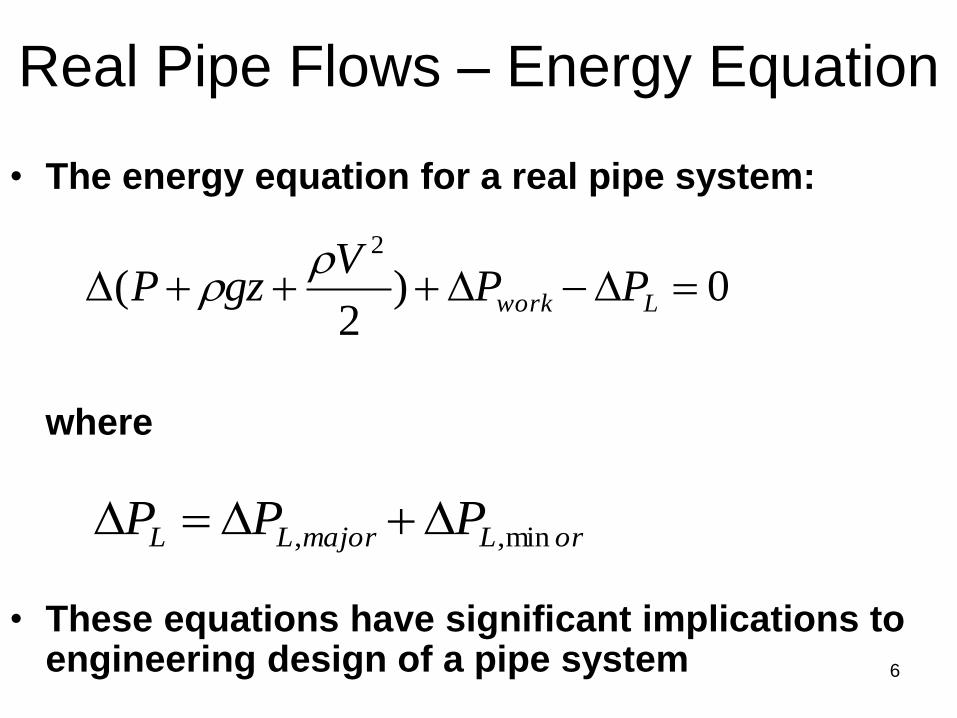
Real Pipe Flows – Energy Equation

• The energy equation for a real pipe system:

where

• These equations have significant implications to engineering design of a pipe system

0)2

(2

Lwork PPV

gzP

orLmajorLL PPP min,,

7

8

Flow Through Circular Conduits

Consider the steady flow of a fluid of constant density in

fully developed flow through a horizontal pipe and

visualize a disk of fluid of radius r and length dL moving

as a free body. Since the fluid posses a viscosity, a shear

force opposing the flow will exist at the edge of the disk

9

Boundary layer buildup in a pipe

Pipe

Entrance

v v v

Because of the share force near the pipe wall, a boundary layer

forms on the inside surface and occupies a large portion of the flow

area as the distance downstream from the pipe entrance increase. At

some value of this distance the boundary layer fills the flow area.

The velocity profile becomes independent of the axis in the direction

of flow, and the flow is said to be fully developed.

10

Laminar vs. Turbulent Flow

• Laminar flow: Fluid flows in smooth layers

and the shear stress is the result of

microscopic action of the molecules.

• Turbulent flow is characterized by large

scale, observable fluctuations in the fluid and

flow properties are the result of these

fluctuations.

11

Real Pipe Flow

Figure 4

12

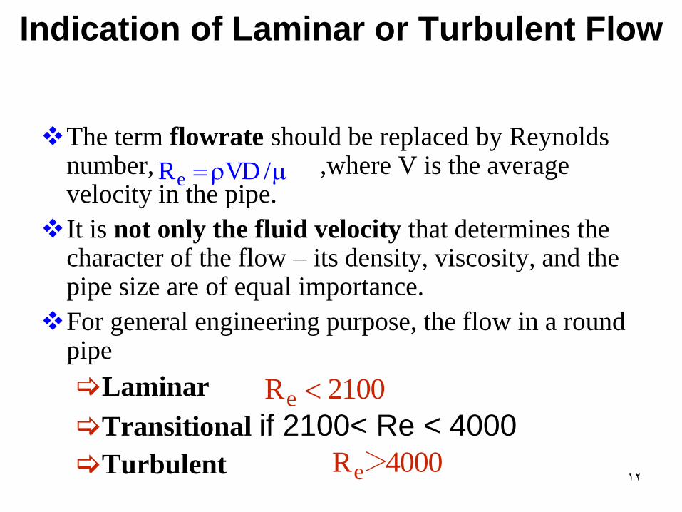
Indication of Laminar or Turbulent Flow

The term flowrate should be replaced by Reynolds number, ,where V is the average velocity in the pipe.

It is not only the fluid velocity that determines the character of the flow – its density, viscosity, and the pipe size are of equal importance.

For general engineering purpose, the flow in a round pipe

Laminar

Transitional if 2100< Re < 4000

Turbulent

/VDRe

2100Re

4000＞Re

13

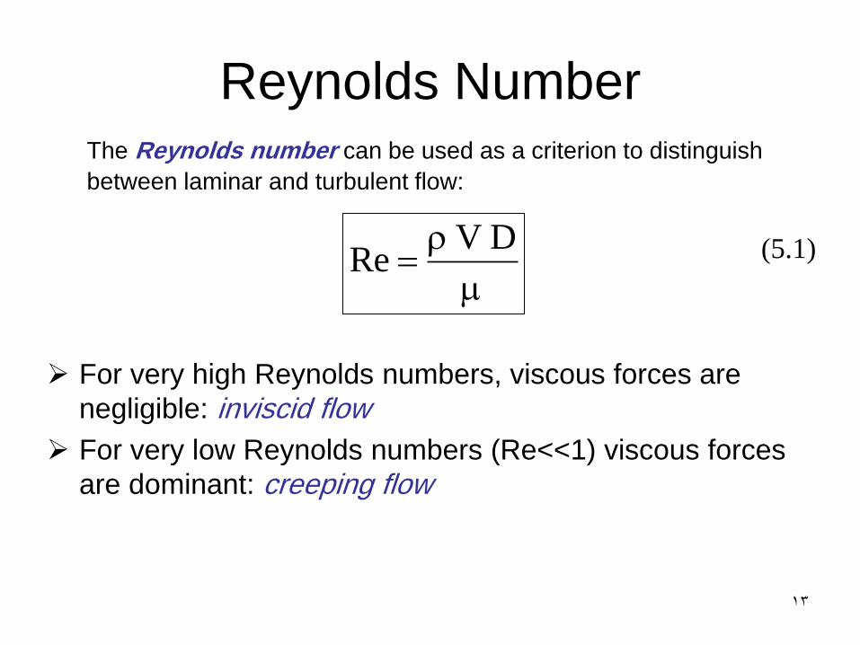
Reynolds Number The Reynolds number can be used as a criterion to distinguish

between laminar and turbulent flow:

For very high Reynolds numbers, viscous forces are

negligible: inviscid flow

For very low Reynolds numbers (Re<<1) viscous forces

are dominant: creeping flow

(5.1)

DV Re

14

Fully Developed Flow

Flow in the entrance region of a pipe is complex.

Once the velocity profile no longer changes, we have reached fully

developed flow. Mathematically dV/dx = 0

Typical entrance length, 20 D < Le < 30 D

15

Entrance Region Flow and Fully

Developed Pipe Flow

Le

We focus on fully developed pipe flow.

16

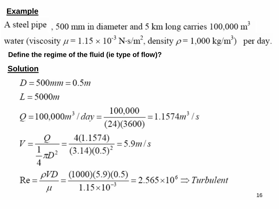
Example

Define the regime of the fluid (ie type of flow)?

Solution

17

18

19

Pressure Driven Flow in pipes

P1

P2

L

20

Forces acting on a fluid

The forces acting on a fluid are divided into two groups:

• Body forces act without physical contact. They act on

every mass element of the body and are proportional to

its total mass. Examples are gravity and electromagnetic

forces

• Surface forces require physical contact (i.e. surface

contact) with surroundings for transmission. Pressure

and stresses are surface forces.

21

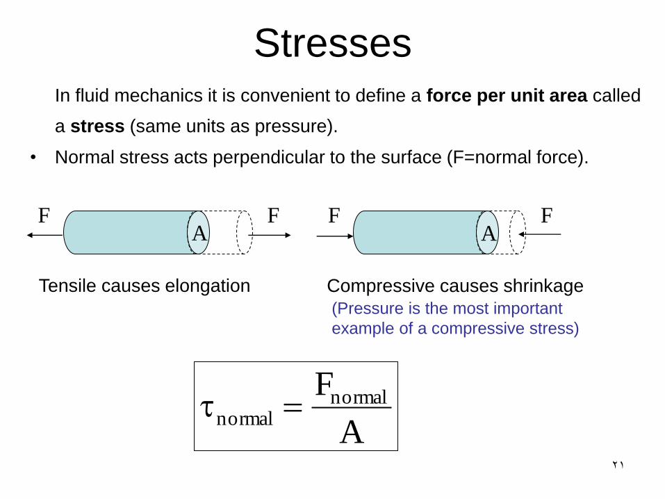
Stresses In fluid mechanics it is convenient to define a force per unit area called

a stress (same units as pressure).

• Normal stress acts perpendicular to the surface (F=normal force).

Tensile causes elongation Compressive causes shrinkage

(Pressure is the most important

example of a compressive stress)

F F F F A A

A

Fnormalnormal

22

Stresses • Shear stress acts tangentially to the surface

(F=tangential or shear force).

F

F A

A

Fshearshear

Recall from chapter 2:

A fluid is defined as a substance that deforms continuously

when acted on by a shearing stress of any magnitude.

23

Shear Stress Profile

Force balance on cylindrical fluid element:

rx

PP

xrrPrP

2)(

02

21

2

2

2

1

x

r

o r

(5.2)

1 2

xrrPrP 2 2

2

2

1

24

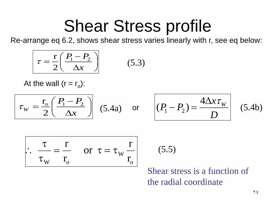
Shear Stress profile

x

PP 21

2

r

Re-arrange eq 6.2, shows shear stress varies linearly with r, see eq below:

At the wall (r = ro):

x

PPW

21o

2

r

o

W

oW r

ror

r

r

Shear stress is a function of

the radial coordinate

or D

xPP W

4

)( 21

(5.3)

(5.4b)

(5.5)

(5.4a)

25

Case one: Laminar flow

To describe any of these flows, conservation of mass and

conservation of momentum equations are the most general forms

could be used to describe the dynamic system. Where the key

issue is the relation between flow rate and pressure drop.

If the flow of fluid is:

a. Newtonian

b. Isothermal

c. Incompressible (dose not depend on the pressure)

d. Steady flow (independent on time).

e. Laminar flow (the velocity has only one single component)

26

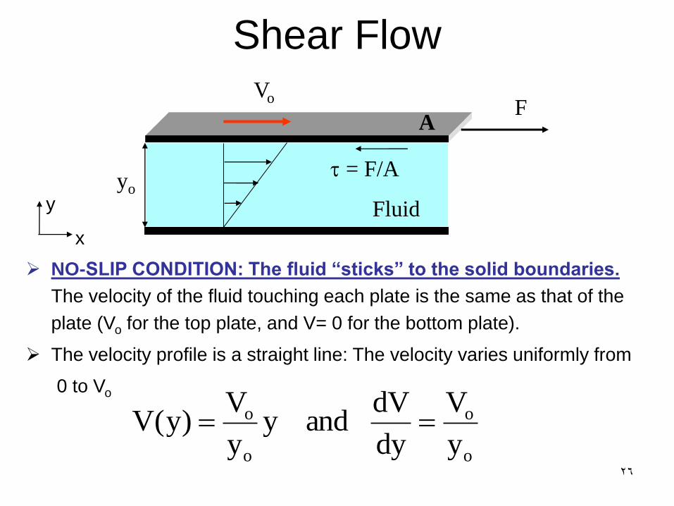
Shear Flow

NO-SLIP CONDITION: The fluid “sticks” to the solid boundaries.

The velocity of the fluid touching each plate is the same as that of the

plate (Vo for the top plate, and V= 0 for the bottom plate).

The velocity profile is a straight line: The velocity varies uniformly from

0 to Vo

Vo

A

yo

Fluid

x

y

F

= F/A

o

o

o

o

y

V

dy

dV and y

y

V)y(V

27

Shear Flow The force, F is proportional to the velocity Vo, the area in contact with

the fluid (A) and inversely proportional to the gap between plates (yo):

y

V AF

o

o

Recall, shear stress, = F / A

y

V

o

o

In the limit of small deformations the ratio Vo/yo can be replaced by the

velocity gradient dV/dy (or dU/dy):

dy

dV

Rate of shearing strain or shear rate:

dy

dV

28

Newton’s law of Viscosity Newton’s law of viscosity

dy

dV

m Viscosity [N/m2 . s =Pa . s]

n = /ρ : Kinematic viscosity [m2/s]

Newtonian fluids: Fluids which obey Newton’s law: Shearing stress is

linearly related to the rate of shearing strain.

(5.6)

The viscosity of a fluid measures its resistance to flow under an

applied shear stress.

29

Laminar Flow: Velocity profile Let’s consider again the flow of a fluid inside a pipe.

In cylindrical coordinates (6.6) can be written:

dr

dV By combining with eq (5.3)

and integrating:

2

o

2

o21

r

r1

x4

r )P-P()r(V

Velocity profile is parabolic

x

)P-P(

4

rr)r(V 21

22

o

[5.8 (a)]

[5.8 (b)]

x

PP 21

2

r

30

Laminar Flow: Velocity profile Minimum velocity, V=0 at the pipe wall (r=ro)

Maximum velocity Vmax at pipe centerline (located at r =0) and

x4

r )P-P(V

2

o21max

The velocity profile can be written:

2

o

maxr

r1 V)r(V

[5.8 (c)]

(5.9)

0dr

du

31

Laminar flow: Velocity and Shear stress

profiles

VELOCITY SHEAR

STRESS

32

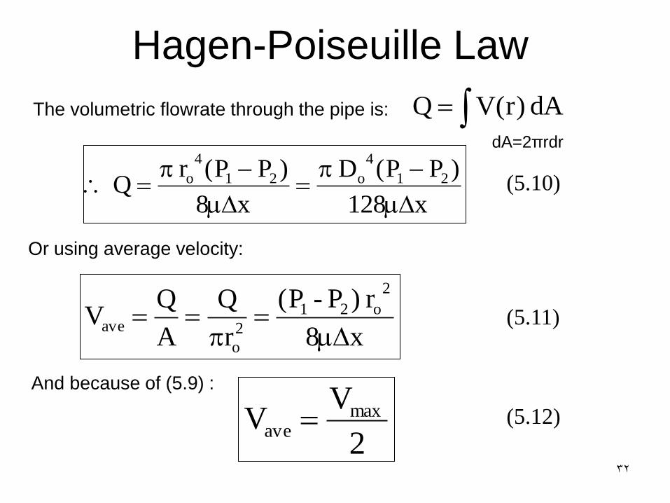
Hagen-Poiseuille Law

dA )r(VQThe volumetric flowrate through the pipe is:

x128

)PP( D

x8

)PP(r Q 21

4

o21

4

o

Or using average velocity:

x8

r )P-P(

r

Q

A

QV

2

o21

2

o

ave

(5.10)

(5.11)

And because of (5.9) :

2

VV max

ave (5.12)

dA=2πrdr

33

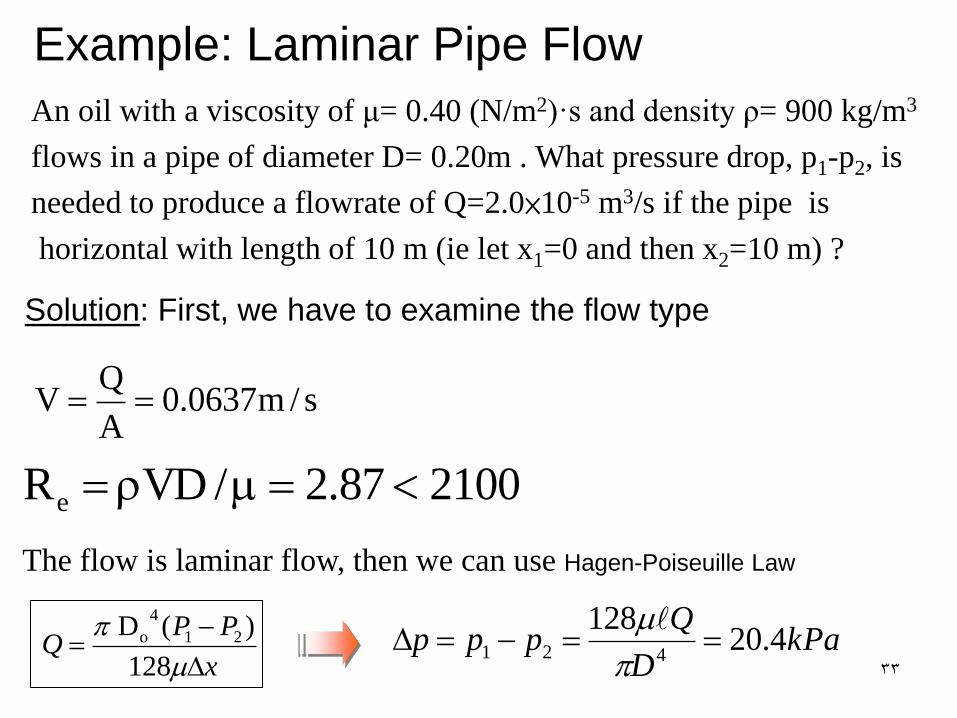
Example: Laminar Pipe Flow

An oil with a viscosity of μ= 0.40 (N/m2)·s and density ρ= 900 kg/m3

flows in a pipe of diameter D= 0.20m . What pressure drop, p1-p2, is

needed to produce a flowrate of Q=2.0×10-5 m3/s if the pipe is

horizontal with length of 10 m (ie let x1=0 and then x2=10 m) ?

Solution: First, we have to examine the flow type

210087.2/VDRe

s/m0637.0A

QV

The flow is laminar flow, then we can use Hagen-Poiseuille Law

kPaD

Qppp 4.20

128421

x

PPQ

128

)(D 21

4

o

34

Example:

pressure of oil in a pipe which discharges into the atmosphere is

measured at a certain location. Assume laminar flow conditions.

The pressure at the distance 15 m found 88 kPa.

(a) The flow rates are to be determined? Proof the flow is laminar.

Properties: The density and dynamic viscosity of oil are given to be = 876

kg/m3 and = 0.24 kg/ms.

(b) If the pipe is designed to produce uphill flow with an inclination of 8,

find flow rates

(c) If the pipe is designed to produce down hill flow with an inclination of 8,

find flow rates

35

2422

21

m 10767.14/m) 015.0(4/

kPa 4788135

DA

PPP

c

/sm 101.62 35

kPa 1

N/m 1000

N 1

m/skg 1

m) s)(15kg/m 24.0(128

m) (0.015kPa) 47(

128

2244

L

DPQ

0.7skg/m 24.0

m) m/s)(0.015 127.0)(kg/m 876(Re

m/s 127.0m 101.767

/sm.1024.2

3

24-

35

VD

AV

c

Q َ

Solution: (a)

Re < 2100 thus it is a laminar flow

36

Q

Q