FLOOD-FLOW FREQUENCY MODEL SELECTION IN

SOUTHWESTERN UNITED STATES

By Richard M. Vogel,l Member, ASCE, Wilbert 0. Thomas Jr.,2 andThomas A. McMahon,3 Member, ASCE

ABSTRACT: Uniform flood frequency guidelines in the United States recommendthe use of the log Pearson type 3 (LP3) distribution in flood frequency investiga-tions. Many investigators have suggested alternate models such as the generalizedextreme value (GEV) distribution as an improvement over the LP3 distribution.Using flood-flow data at 383 sites in the southwestern United States, we explorethe suitability of various flood frequency models using L-moment diagrams. Wealso repeat the experiment performed in the original Water Resource Council report(Bulletin 17B, issued in 1982), which led to the LP3 mandate. All our evaluationsconsistently reveal that the LP3, GEV, and the two- and three-parameter lognormalmodels (LN2 and LN3) provide a good approximation to flood-flow data in thisregion. Other models such as the normal, Pearson, and Gumbel distributions areshown to perform poorly. Recent research indicates that regional index-flood pro-cedures should be more accurate and more robust than the type of at-site proceduresevaluated here. Nevertheless, this study reveals that index-flood procedures neednot be restricted to the GEV distribution because the LN2, LN3, and LP3 distri-butions appear to be suitable alternatives, at least in the southwestern United States.

INTRODUCTION

Many innovations in the field of flood frequency analysis have occurredsince the decision of the U.S. Water Resources Council (1967) to recom-mend the use of the log Pearson type 3 (LP3) distribution for flood-flowinvestigations in the United States. The state of the art of selecting a regionalflood frequency distribution at the time of the LP3 mandate was considerablydifferent from the current situation. For example, in describing the U.S.Water Resource Council (WRC) work group study. ("Guidelines" 1967),Benson (1968) argued that "no single method of testing [alternative hy-potheses] was acceptable to all those on the Work Group, and the statisticalconsultants could not offer a mathematically rigorous method," leading tothe conclusiqn that "there are no rigorous statistical criteria on which tobase a choice of method."

More recently, L-moment diagrams and associated goodness-of-fit pro-cedures (Hosking and Wallis 1987; Wallis 1988; Cunnane 1989; Hosking1990; Chowdhury et al. 1991; Vogel and Fennessey 1993; Vogel et al. 1993)were advocated for evaluating the suitability of selecting various distribu-tional alternatives in a region. For example, Hosking and Wallis (1987)found L-moment diagrams useful for selecting the generalized extreme valuedistribution (GEV) over the Gamma distribution for modeling annual max-imum hourly rainfall data. Similarly, Wallis [(1988), Fig. 3] found an L-moment diagram useful for rejecting Jain and Singh's (1987) conclusion thatannual maximum flood flows at 44 sites were well approximated by a Gumbeldistribution and for suggesting a GEV distribution instead.

lAssoc. Prof., Dept. of Civ. Engrg., Tufts Univ., Medford, MA 02155.2Hydro., U.S. Geolog. Survey, 12201 Sunrise Valley Dr., Reston, VA 22092.JProf., Univ. of Melbourne, Parkville, Victoria 3052, Australia.Note. Discussion open until October 1, 1993. To extend the closing date one

month, a written request must be filed with the ASCE Manager of Journals. Themanuscript for this paper was submitted for review and possible publication on April8, 1992. This paper is part of the Journal of Water Resources Planning and Manage-ment, Vol. 119, No.3, May/June, 1993. @ASCE, ISSN 0733-9496/9310003-03531$1.00+ $.15 per page. Paper No.3787.

353

Another approach for evaluating the fit of alternate probability modelsand associated parameter estimation schemes is nonparametric experimentsof the type performed by Beard (1974) and summarized by the InteragencyAdvisory Committee on Water Data (IACWD) ["Guideline" (1982), Ap-pendix 14]. Using 300 stations distributed across the United States, Beardcounted the number of stations for which the estimated 1,000-yr flood flowwas exceeded in the historical record. Eight independent methods wereemployed for estimating the 1,000-yr flood at each site; results are repro-duced in Table 1. Beard argued that with a total of n = 14,200 station-years of data across the 300 sites, one would expect approximately 14 ex-ceedances of the true 1,000-yr flood flow. Only the LP3 and LN2 distri-butions came close to reproducing the 14 expected exceedances. Beard(1974) performed many other tests, but it was this test that convinced hy-drologists that both the LP3 and LN2 models approximate the distributionof observed flood-flow data throughout the entire United States.

A third approach to evaluating the fit of alternative probability modelsto a regional data base is to employ probability plots and associated prob-ability plot correlation coefficient (PPCC) tests (Vogel 1986; Vogel andKro111989; Vogel and McMartin 1991; Chowdhury et al. 1991). Such testsare usefu., simple, and powerful for most two-parameter distributional al-ternatives, (VogeI1986; Vogel and KrollI989). However, Vogel and McMartin(1991) show that a PPCC test for the LP3 distribution exhibits remarkablylow power in discriminating against similar distributional hypotheses.Chowdhury et al. (1991) arrived at similar conclusions for the GEVPPCCtest. We elected not to perform PPCC hypothesis tests here due to the likelyambiguity of such test results for the three-parameter alternatives consid-ered.

In the following sections, we employ L-moment diagrams and Beard'snonparametric test to annual maximum flood-flow data in the southwesternUnited States. Our goal is to both assess the adequ.acy of the existing LP3flood frequency procedures and to choose other plausible procedures forapproximating the underlying distribution of flood flows in this region.

STUDY REGION

The annual maximum flood-flow data employed in this study include 383U.S. Geological Survey gaging stations with unregulated streamflow recordlengths of 30 or more years. These stations are located in the 10-state region

TABLE 1. Number of Stations Where One or More Observed Flood Events Ex-ceeds 1,OOo-Yr Flood Flow

Method Number of exceedances(1) (2)

Log Pearson type 3 (LP3) 14Lognormal (LN2) 18Gumbel (MLE estimators) 77Log Gumbel 1Gamma 68Pearson type 3 (P3) 56Regionallog Pearson type 3 20Gumbel (best linear invariant estimator) 253

Note: From Beard (1974) and IACWD ["Guidelines" (1982), Table 14-2].

354

.9"-- ,20" C A N A D A, --, ',8' ,00'

r,- : -r 7-7 "2. 108' 104' " --, ' ' r T 7 r T '-.- 1

, > , ' I' ,.' , , ., I" ' .1 ti1'- '7WASH ti' I ' NO"T

.GTON ! " \ D~KOTA

I' ',. M o N T A N A \

r IDAHOI ,.5' .' , .r

I '-i I

: .:/ " , 1

1-:

I

:---I

.1':-

.'

'\

L

'\ "

jj31*"

~ ,

~ .

')0

~

Basa from ARC/INFO

0 100 MILESf-.'rJT,.J0 loo KILOMETERS

FIG. 1. Ten-State Study Region in Southwestern United States

of the southwestern United States shown in Fig. 1. The 383 stations are a

subset of the 1,059 stations employed by Thomas et al. (1992) for developing

regional hydrologic equations for estimating floodflow quantiles in this 10-

state region. Our data base is considerably smaller than the one used by

Thomas et al. (1992) because we only considered sites with records longer

than 30 years; and we rejected sites that contained annual maximum flood

flows equal to zero. Sites that contained annual maximum flood flows equal

to zero were rejected so that our goodness-of-fit evaluations would not be

confounded by methods for the treatment of zeros, which would have been

required had we included these sites. Fig. 2 illustrates the distribution of

record lengths, with an average length of 50 yr .The basins with longer records in the southwestern United States tend

to be operated for water supply purposes, hence such basins contain higher

base flow runoff than short-record sites. Since we dropped sites with zero

annual maximum flood flows, and since we only used sites with longer

records (n ?; 30 yr), the data base employed here consists of mostly larger,

less arid basins in the arid southwestern United States. We would have liked

to include the smaller, more arid basins since such basins exhibit the most

variable streamflow and pose the greatest hydrologic modeling challenge.

355

.9"-- ,20" C A N A D A, --, ',8' ,00'

r,- : -r 7-7 "2. 108' 104' " --, ' ' r T 7 r T '-.- 1

, > , ' I' ,.' , , ., I" ' .1 ti1'- '7WASH ti' I ' NO"T

.GTON ! " \ D~KOTA

I' ',. M o N T A N A \

r IDAHOI ,.5' .' , .r

I '-i I

: .:/ " , 1

1-:

I

:---I

.1':-

.'

'\

L

'\ "

jj31*"

~ ,

~ .

')0

~

Basa from ARC/INFO

0 100 MILESf-.'rJT,.J0 loo KILOMETERS

FIG. 1. Ten-State Study Region in Southwestern United States

of the southwestern United States shown in Fig. 1. The 383 stations are a

subset of the 1,059 stations employed by Thomas et al. (1992) for developing

regional hydrologic equations for estimating floodflow quantiles in this 10-

state region. Our data base is considerably smaller than the one used by

Thomas et al. (1992) because we only considered sites with records longer

than 30 years; and we rejected sites that contained annual maximum flood

flows equal to zero. Sites that contained annual maximum flood flows equal

to zero were rejected so that our goodness-of-fit evaluations would not be

confounded by methods for the treatment of zeros, which would have been

required had we included these sites. Fig. 2 illustrates the distribution of

record lengths, with an average length of 50 yr .The basins with longer records in the southwestern United States tend

to be operated for water supply purposes, hence such basins contain higher

base flow runoff than short-record sites. Since we dropped sites with zero

annual maximum flood flows, and since we only used sites with longer

records (n ?; 30 yr), the data base employed here consists of mostly larger,

less arid basins in the arid southwestern United States. We would have liked

to include the smaller, more arid basins since such basins exhibit the most

variable streamflow and pose the greatest hydrologic modeling challenge.

355

A4 .T4=~=L-kurtOSlS (lc)

where Ar, r = 1, ..., 4 = first four L-moments; and T2' T3, and T4 = L-coefficient of variation (L-Cv), L-skewness, and L-kurtosis, respectively.The first L-moment, At, is equal to the mean IJ., hence it is a locationparameter. Hosking (1990) shows that A2, T3, and T4 can be thought of asmeasures of a distributions scale, skewness, and kurtosis, respectively, anal-ogous to the ordinary moments a, "Y, and K, respectively.

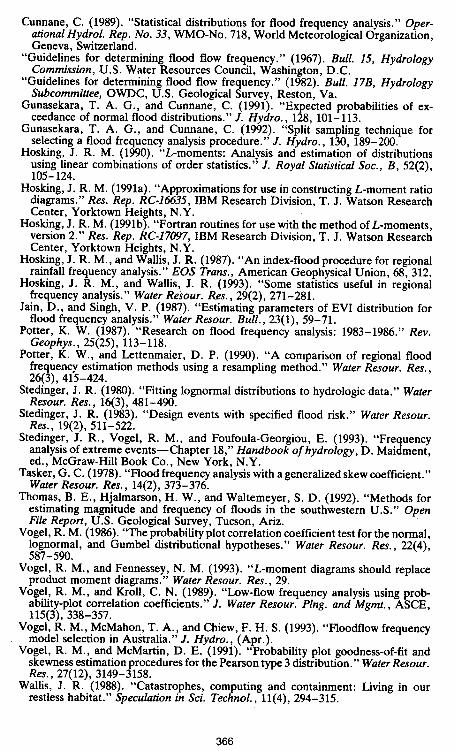
L-Moment DiagramsAn L-moment diagram compares sample estimates of the dimensionless

ratios, T2, T3, T4, with their population counterparts for a range of assumeddistributions. An advantage of L-moment diagrams is that one can comparethe fit of several distributions using a single graphical instrument. Fig. 3compares the relationship between nearly unbiased sample estimates of T4and T3 (using open circles) anQ their population values. Here, sample es-timates of T2 , T3 , and T4 are obtained using the unbiased probability-weightedmoment estimators of At, A2, A3, and A4 as recommended by Stedinger etal. (1993), when constructing L-moment diagrams. Unbiased probabilityweighted moment estimators are equivalent to the unbiased L-moment es-timators introduced by Hosking (1990). However, use of unbiased esti-mators of the sample L-moment Ar, r = 1, ..., 4, does not imply that theL-moment ratio estimators TI' i = 1, 2, and 3, are unbiased. Fig. 3(a) wasconstructed using annual maximum flood flow data for the 383 sites de-scribed previously. The true relationships between L-kurtosis and L-skew-ness corresponding to the Pearson type 3 (P3), LN3, GEV, Gumbel, andnormal distributions are shown for comparison in Fig. 3. These theoreticalrel1itionships are summarized in Hosking (1991a) and Stedinger et al. (1993)hence we only report the theoretical relationships "for normal (T3 = 0; T4 =0.1226) and Gumbel (T3 = 0.1699; T4 = 0.1504) distributions since theircoordinates are difficult to discern amidst the scatter of points in Fig. 3.

Fig. 3(a) reveals that of the models tested, only the LN3 and GEVdistributions appear consistent with this regional sample, and of those twodistributions, it appears that the LN3 model provides the better fit to thedata. Roughly half the observations are above the LN3 line and half arebelow; there are fewer than half the observations above the GEV line.

Unfortunately, a theoretical relationship between L-kurtosis and L-skew-ness is unavailable for the LP3 distribution. Since such a theoretical rela-tionship only exists for the P3 distribution, we synthetically generated LP3,LN3, GEV, normal, and P3 samples for comparison in Fig. 3(b-.n, re-spectively. We generated 383 independent samples of LP3, LN3, GEV,normal, and P3 data with record lengths equal to record lengths of theobserved flood-flow data in Fig. 3(a). In generating the synthetic samplesat each site, we assumed that population values of each model parameterequaled the sample estimates obtained at each site. The purpose of usingdifferent population parameters at each site was to attempt to capture thehydrologic heterogeneity of flood flows across the region. The character ofgenerated LP3, LN3, and GEV samples displayed in Fig. 3(b-d) appearsto be very similar to the observed floodflow samples in Fig. 3(a), yet thecharacter of generated normal and P3 samples is quite different from theobserved flood-flow samples in Fig. 3(a).

In Fig. 4 we plot estimates of L-kurtosis versus estimates of L-skewness

357

1.00.9 o noodfiow Data

I --P30.8 -W3

-0.7 0 ~ crn GEV cO0.6

rn .Gumb.lO 0.5

No"mal~ 0.4

;j 03~I 0.2

~ 0.10.0

-0.1(a) -0.1 0.0 0.1 0.2 0.3 0.4 0.5 0.6 0.7 0.8

1.00.9 o LP3 Synlhetlc Data

P31- 0.6 -W3

-0.7 "rn GEV 0-;

0.6rn .Gumb.lO 0.5

No"mal~ 0.4

;j 0.3~I 0.2

~ 0.1 o0.0

-0.1(b) -01 0.0 0.1 0.2 0.3 0.4 0.5 0.6 0.7 0.8

1.00.9 o lJI3 Synth.lic Dala

1 --P30.8 -lJI3

-0.7rn GEV c0.6

rn .GumbelO 0.5

No"mal~ 0.4:j 0.3

~I 0.2~ 01 o o

0.0 o o

-0.1(c) -0.1 0.0 0.1 0.2 0.3 0.4 0.5 0.6 0.7 0.8

L-Skewness, T3

FIG. 3. L-Moment Diagrams of: (B) Observed Annual Maximum Floodflow Data;(b) Synthetic Log Pearson Type 3 (LP3) Data; (c) Synthetic Three-Parameter Log-normal (LN3) Data

356

using logarithms of the annual maximum flood flows. For comparison, weplot the theoretical relationship for P3 data, which provides a test on whetherthe distribution of the logarithms of flood-flow data resembles a P3 distri-bution, which is equivalent to checking whether the distribution of the floodflows resembles an LP3 distribution. Since the average skewness of thelogarithms in this region is approximately zero, it is not surprising that thedata cluster around the value T4 = 0.1226 and T3 = 0, which correspondsto the population values for an LN2 distribution. Here again, in Fig. 4(band c), we compare synthetic LP3 and synthetic LN3 data, respectively.Similar to Fig. 3, Fig. 4 documents that both synthetic LP3 and syntheticLN3 data behave much like the original flood-flow data.

From all our comparisons in Figs. 3 and 4, we conclude that observedflood-flow samples are well approximated by LP3, LN2, LN3, and GEVprobability distributions, yet are poorly approximated by a P3, normal, orGumbel distribution. Our conclusions are derived from a subjective graph-ical evaluation of the goodness of fit of alternative distributions. Hoskingand Wallis (1993) describe more objective quantitative goodness-of-fit pro-cedures that may be employed in association with L-moment diagrams.

NONPARAMETRIC EVALUATION OF FLOOD-FREQUENCY PROCEDURES

The previous L-moment diagrams focused on the ability of alternativeprobability models to approximate the distribution of flood flows; however ,those comparisons did not evaluate the ability of alternative methods toprovide estimates of design quantiles. In this section we evaluate the per-formance of alternative models and parameter-estimation schemes in termsof their ability to predict the 100- and 1,000-year flood flows. We repeat aportion of the experiment performed by Beard (1974) and summarized inTable 1 and in IACWD ("Guidelines" 1982), which led to the originaluniform flood-frequency guidelines in the United States. The experiment isconceptually simple and focuses on the important question of how well eachmodel and associated parameter-estimatio"n scheme performs in terms ofpredicting extreme flood flows with a fixed exceedance probability.

Flood-Flow Frequency Methods EvaluatedThe experiment begins by estimating the 100- and 1,000-yr flood flow at

each of the 383 sites using the following methods.

Log Pearson Type 3 Distribution ( LP3 )The method of moments in log space, as recommended by IACWD

("Guidelines" 1982) is always used for estimating the mean and varianceof the logarithms. Four different methods are considered for estimating theskew of the logarithms.

1. LP3-'Y = 0: The skew is always set to zero.2. LP3-G1: The at-site skew estimator described in IACWD ("Guide-

lines" 1982) is used.3. LP3-G,: The at-site probability plot correlation coefficient skew esti-

mator described by Vogel and McMartin (1991) is used.4. LP3-Gw: The weighted skew estimator described in IACWD ("Guide-

lines" 1982) is used where the regional skew is assumed to be zero with amean square error of 0.31. Thomas et al. (1992) found that the mean squareerror associated with four alternate regional estimators of the skew coef-

361

ficient for this lo-state region [including the regional map skew from IACWD("Guidelines" 1982)] were all about equal to the mean square error of thesample of 1,059 gaged records, which was 0.31. Their tests failed to rejectthe hypothesis that the regional population skew is zero. Hence, Thomaset al. (1992) recommend assuming a fixed regional skew of zero for theentire region and using Tasker's (1978) recommended formula [also seeIACWD ("Guidelines" 1982), pages 12-13] for obtaining a weighted esti-mator of the at-site skew coefficient and the regional skew. Here, the meansquare error of the regional skew coefficient is assumed to be 0.31. We termthis skewness estimator Gw.

Lognormal DistributionTwo procedures are considered. The two-parameter lognormal procedure

(LN2) employs maximum likelihood estimators and the three-parameterlognormal procedure (LN3) employs Stedinger's (1980) estimator of thelower bound ~ along with sample estimators of the mean and variance of Yi= In (xi -~), where xi are the observed flood flows. Stedinger (1980) andStedinger et al. (1993) summarize these procedures.

Generalized Extreme Value DistributionThe generalized extreme value (GEV) procedure and the Gumbel or

extreme value type I procedures (GUM) were also examined. These pro-cedures employ unbiased L-moment estimators of each distributions pa-rameters as described in Stedinger et al. (1993).

Expected Probability AdjustmentMost quanti le estimators provide almost unbiased estimates of the per-

centile of interest. Hence, one expects, on average, the estimated 100- and1,000-yr events to equal their population values. However, an unbiasedestimator of the T -yr event will not, in general, be exceeded with an averageprobability of p = I/T. Beard (1960), Beard (1978), IACWD ["Guidelines"(1982), Appendix 11], Stedinger (1983), Gunasekara and Cunnane (1991),and Stedinger et al. (1993) discuss this issue in greater detail.

For normal and lognormal samples, Bulletin 17B [IACWD ("Guidelines"1982), Appendix 11] provides formulas for the probabilities that an almostunbiased quantile estimator of the T -yr event will be exceeded. For example,for the T = 1 ,000-yr event, the expected exceedance probability is 0.001(1.0+ 280/N1.sS), and for the T = 100-yr event the expected exceedance prob-ability isO.01(1.0 + 26/Nl.16), for normal samples. Note that, for the averagesample size employed here (n = 50), expected exceedance probabilities forT = 1,000 and T = 100-yr events are 0.00165 and 0.0128, :espectively,instead of 0.001 and 0.01. Although these corrections were derived for thenormal and lognormal distributions, they have been recommended by IACWD("Guidelines" 1982) for use with the LP3 distribution. We employ thesecorrections for all of the methods considered. Gunasekara and Cunnane(1991) showed that the expected probability correction for normally dis-tributed samples is approximately valid for other distributions.

Experimental ProcedureUsing each of the foregoing methods, we counted the number of times

an observed annual maximum floodflow exceeded the estimated T = 100

362

and T = 1,000-yr flood flow with and without the use of an expectedprobability adjustment. The results are reported in Table 2. If one assumesthat the 383 sites are independent, and that floods occur independently fromone year to the next at each site, then the number of exceedances, X, followsa binomial distribution with mean E[X] = mp and variance Var[X] =mp(l -p ), where m is the number of independent trials and p is theexceedance probability associated with each event (p = l/T). There are m= 19,196 site-years of data (or independent trials) across the 383 sites.Hence, on avera~e, over many such experiments, one expects to observeapproximately ElX] = 19 and E[X] = 192 exceedances of the 1,000- and100-yr events, respectively. Furthermore, since X follows a binomial dis-tribution, we can estimate the 95% likely interval as the range of valuesone might expect (95% of the time) over repeated experiments of this kind.The 95% intervals (XO.025 , XO.97S) are reported in Table 2 and are found from

xO.97' ( )0.95 = ~ m px(l-p)m-x (2)x-XO02S X

where m = 19,196 and p = 0.01 and 0.001 for the 100- and 1,000-yr events,

respectively.

ResultsTable 2 reports the number of observed flood flows, out of the entire

sample of m = 19,196 site-yrs of flood flows that exceeded the 100- and1,000-yr events. We document the results with and without the expectedprobability adjustment corresponding to eight different methods. The onlyprocedure that leads to observed exceedances that always fall within the95% likely interval, both with and without th.e expected probability ad-justment, is the LP3-Gw method, the method recommended by IACWD

TABLE 2. Number of Observed Flood Flows that Exceed 100- and 1,000-Yr FloodFlow Computed from Each Station's Complete Record Using Eight Different Meth-ods.

NUMBER OF EXCEEDANCES

T = 100 T = 1,000

No expected Expected No expected Expectedprobability probability probability probability

Method adjustment adjustment adjustment adjustment(1) (2) (3) (4) (5)

LP3-'Y = 0 176" 217. 25. 34LP3-G, 244 292 75 88LP3-Gr 164 210" 45 52LP3-Gw 172. 216. 18. 26"LN2 165. 207. 21. 33LN3 172. 229 816"GEV 152 215. 11. 13.GUM 377 443 132 161

Theoretical expectation 192 192 19 1995% likely interval (165, 219) (165, 219) (11, 28) (11, 28)

.Results fall inside 9~% likely interval.

363

(.'Guidelines" 1982). The only methods leading to observed exceedancesthat always fall within the 95% likely interval with the expected probabilityadjustment are the LP3-Gw and the GEV procedures. Since an expectedprobability adjustment is required to reproduce the theoretical expectationand to produce results that fall within the 95% likely interval of the numberof exceedances we place greater weight on the results with the expectedprobability adjustment. Unfortunately, an exact expected probability ad-justment is unavailable for the GEV and LP3 methods, hence our resultsfor those cases are approximate .

For the T = 1,000-yr event, the LP3-Gw , LN3, and GEV procedures arethe only methods that produce exceedances that fall within the 95% likelyinterval when the expected probability adjustment is made. This result agreeswith our previous conclusions based on L-moment diagrams, which showedthat these distributions seemed to behave most like the observed flood-flowsamples. For the T = 100-yr event, similar results are obtained since nowthe LP3-"y = 0, LP3-G" LP3-Gw, LN2, and GEV procedures are the onlymethods that produce exceedances that fall within the 95% likely intervalwhen the expected probability adjustment is made.

Vogel and McMartin (1991) showed that the at-site PPCC skew estimatorG, should always perform as well or better than the at-site skew estimatorGl. This result is verified in Table 2, which reveals that the LP3-G, pro-cedure was always an improvement over the LP3-Gl procedure.

Unfortunately, experiments such as the one reported in Table 2 can neverbe definitive, because actual flood-flow samples are cross correlated in space.Cross correlation reduces the amount of regional experience, implying thatone needs more basins to obtain convergence between the theoretical num-ber 'of exceedances and the observed number of exceedaAces. Cross cor-relation of the flood-flow samples implies that there are effectively fewerthan 19,196 independent samples leading to a wider 95% likely interval thanis reported in Table 2.

Interestingly, Gunasekara and Cunnane (1992) reached almost identical.conclusions to ours by repeating Beard's experiment with synthetic flood-

flow data. Gunasekara and Cunnane (1992) generated 40-yr synthetic flood-flQw traces at 300 artificial sites from seven different parent probabilitydistributions. They employed 13 different model/parameter estimation pro-cedures to estimate the 10-, 100-, and 1,000-yr flood flow at each site. Theyfound that for both the 100- and 1,000-yr events, the regional LP3-Gw andthe at-site GEV procedures employed here reproduced the expected numberof exceedances better than any of the procedures they evaluated. Thoseresults are identical to ours except that we also found that the LN2 and LN3procedures performed well. Gunasekara and Cunnane (1992) did not con-sider the LN3 procedure, and the reason they rejected the LN2 procedurewas probably due to the fact that the logarithms of their artificial samplesexhibited nonzero skew, unlike the logarithms of observed flood flows inthis study.

CONCLUSIONS

The primary objective of this study was to evaluate the ability of severaldistributional alternatives for modeling annual maximum flood flows in a10-state region of the southwestern United States. L-moment diagrams re-vealed that the log Pearson type 3 (LP3), lognormal (LN2), three-parameterlognormal (LN3), and generalized extreme value (GEV) distributions all

364

provide equally acceptable approximations to the observed distribution offlood flows at 383 sites in the region depicted in Fig. 1.

To assess the ability of alternative flood-frequency models and parameter-estimation schemes to estimate design quantiles, we also repeated a portionof the original nonparametric experiment performed by Beard (1974), whichled to the IACWD ("Guidelines" 1982) mandate to recommend the LP3-Ow procedure in the United States. Those experiments also document thatthe LP3-0w, LN2, LN3, and GEV procedures are all equally acceptableprocedures for modeling flood flows in this region. These conclusions aresurprisingly similar to the results of a recent study by Gunasekara andCunnane (1992) that employed synthetic flood-flow data instead of flood-flow observations.

It is satisfying to report that all our evaluations consistently reach similarconclusions. Yet these results do not imply that the current IACWD("Guidelines" 1982) guidelines are satisfactory .Recent studies by Potterand Lettenmaier (1990) and others demonstrate that regional index-floodprocedures for the GEV distribution with L-moment estimators should bemore accurate and more robust than the type of at-site procedures describedhere and recommended by IACWD ("Guidelines" 1982). Stedinger et al.(1993) summarize index-flood procedures. Nevertheless, this study revealsthat index-flood procedures need not be restricted to the GEV distributionbecause the LN2, LN3, and LP3 distributions are suitable alternatives, atleast in the southwestern United States.

Finally, we emphasize, as Potter (1987) and others did that improvementsin regional flood-frequency analysis are usually derived from at-site pro-cedures because the single-site (at-site) model lies at the heart of all regionalprocedures. Since this study focuses on the adequacy of various distribu-tional hypotheses, treating each site independently, our analyses could notreveal any information regarding the adequacy of regional procedures thatexploit the GEV, LN2, LN3, or LP3 distributions. We suggest, however ,that future studies that seek to develop improved regional flood frequencyprocedures consider using the GEV, LN2, LN3, LP3, and possibly otherprocedures as the basis for such methods.

ACKNOWLEDGMENTS

We are grateful to Michael Hynes for his assistance with the computerprogramming. We are also grateful to J. R. Wallis and L. R. Beard fortheir comments on an earlier version of this manuscript. This research wassupported by the University of Melbourne and Tufts University, and it wascompleted while the first writer was on sabbatical leave in Melbourne,Australia.

ApPENDiX. REFERENCES

.Beard, L. R. (1960). "Probability estimates based on small normal-distribution sam-ples." I. Geophys. Res., 65(7), 2143-2148.

Beard, L. R. (1974). "Flood flow frequency techniques." Center for Research inWater Resources, Univ. of Texas at Austin, Austin, Tex.

Beard, L. R. (1978). "Impact of hydrologic uncertainties on flood insurance." I.Hydr. Div., ASCE, 104(11), 1473-1483.

Benson, M. A. (1968). "Uniform flood-frequency estimating methods for federalagencies." Water Resour. Res., 4(5), 891-908.

Chowdhury, J. U., Stedinger, J. R., and Lu, L. (1991). "Goodness-of-fit tests forregional GEV flood distributions." Water Resour. Res., 27(7), 1765-1776.

365

Cunnane, C. (1989). "Statistical distributions for flood frequency analysis." Oper-ational Hydrol. Rep. No.33, WMO-No. 718, World Meteorological Organization,Geneva, Switzerland.

"Guidelines for determining flood flow frequency." (1967). Bull. 15, HydrologyCommission, U.S. Water Resources Council, Washington, D.C.

"Guidelines for determining flood flow frequency." (1982). Bull. 17B, HydrologySubcommittee, OWDC, U.S. Geological Survey, Reston, Va.

Gunasekara, T. A. G., and Cunnane, C. (1991). "Expected probabilities of ex-ceedance of normal flood distributions." J. Hydro. , 128, 101-113.

Gunasekara, T. A. G., and Cunnane, C. (1992). "Split sampling technique forselecting a flood frequency analysis procedure." J. Hydro., 130,189-200.

Hosking, I. R. M. (1990). "L-moments: Analysis and estimation of distributionsusing linear combinations of order statistics." J. Royal Statistical Soc., B, 52(2),105-124.

Hosking, I. R. M. (1991a). "Approximations for use in constructing L-moment ratiodiagrams." Res. Rep. RC-I6635, IBM Research Division, T. I. Watson ResearchCenter, Yorktown Heights, N.Y.

Hosking, I. R. M. (1991b). "Fortran routines for use with the method of L-moments,version 2." Res. Rep. RC-17097, IBM Research Division, T. I. Watson ResearchCenter, Yorktown Heights, N. Y.

Hosking, I. R. M., and Wallis, I. R. (1987). " An index-flood procedure for regional

rainfall frequency analysis." EOS Trans., American Geophysical Union, 68,312.Hosking, I. R. M., and Wallis, I. R. (1993). "Some statistics useful in regional

frequency analysis." Water Resour. Res. ,29(2), 271-281.lain, D., and Singh, V. P. (1987). "Estimating parameters of EVI distribution for

flood frequency analysis." Water Resour. Bull., 23(1),59-71.Potter, K. W. (1987). "Research on flood frequency analysis: 1983-1986." Rev.

Geophys., 25(25),113-118.Potter, K. W., and Lettenmaier, D. P. (1990). "A comparison of regional flood

frequency estimation methods using a resampling method." Water Resour. Res.,26(3), 415-424.

Stedinger, I. R. (1980). "Fitting lognormal distributions to hydrologic data. " WaterResour. Res. , 16(3), 481-490.

Stedinger, I. R. (1983). "Design events with specified flood risk. " Water Resour.

Res. , 19(2), 511-522.Stedinger, I. R., Vogel, R. M., and Foufoula-Georgiou, E. (1993). "Frequency

analysis of extreme events-Chapter 18," Handbook of hydrology, D. Maidment,ed., McGraw-Hill Book Co., New York, N.Y.

Tasker, G. C. (1978). "Flood frequency analysis with a generalized skew coefficient."Water Resour. Res. , 14(2), 373-376.

Thomas, B. E., Hjalmarson, H. W., and Waltemeyer, S. D. (1992). "Methods forestimating magilitude and frequency of floods in the southwestern U .S." OpenFile Report, U.S. Geological Survey, Tucson, Ariz.

Vogel, R. M. (1986). "The probability plot correlation coefficient test for the normal,lognormal, and Gumbel distributional hypotheses." Water Resour. Res. , 22(4),587-590.

Vogel, R. M., and Fennessey, N. M. (1993). "L-moment diagrams should replaceproduct moment diagrams." Water Resour. Res., 29.

Vogel, R. M., and Kroll, C. N. (1989). "Low-flow frequency analysis using prob-ability-plot correlation coefficients." J. Water Resour. Ping. and Mgmt. , ASCE,115(3),338-357.

Vogel, R. M., McMahon, T. A., and Chiew, F. H. S. (1993}. "Floodflow frequencymodel selection in Australia." J. Hydro., (Apr.).

Vogel, R. M., and McMartin, D. E. (1991). "Probability plot goodness-of-fit andskewness estimation procedures for the Pearson type 3 distribution." Water Resour.Res. , 27(12), 3149-3158.

Wallis, I. R. (1988). "Catastrophes, computing and containment: Living in ourrestless habitat." Speculation in Sci. Technol. , 11(4),294-315.

366