Flight and passenger delay assignment optimization strategies · Flight and passenger delay...

Flight and passenger delay assignment optimizationstrategies

A. MontlaurEscola d’Enginyeria de Telecomunicacio

i Aeronautica de CastelldefelsUniversitat Politecnica de Catalunya, Spain

Email: [email protected]

L. DelgadoDepartment of Planning and Transport

University of WestminsterLondon, United Kingdom

Email: [email protected]

Abstract

This paper compares different optimization strategies for the minimization of flight and passenger delays at two levels: pre-tactical, with on-ground delay at origin, and tactical, with airborne delay close to the destination airport. The optimization modelis based on the ground holding problem and uses various cost functions. The scenario considered takes place in a busy Europeanairport and includes realistic values of traffic. A passenger assignment with connections at the hub is modeled. Statistical modelsare used for passenger and connecting passenger allocation, minimum time required for turnaround and tactical noise; whereasuncertainty is also introduced in the model for tactical noise. Performance of the various optimization processes is presented andcompared to ration by schedule results.

Index Terms

Air Traffic Flow Management; Integer programming; Flight and passenger delay; E-AMAN; Pre-tactical optimization

1

Flight and passenger delay assignment optimizationstrategies

I. INTRODUCTION

Airports are limited in capacity by operational constraints (Bazargan et al., 2002; Gilbo, 1993; Hinton et al., 2000; Groskreutzand Munoz-Dominguez, 2015). In some cases, a significant imbalance exists between capacity and demand. Air Traffic Flowand Capacity Management (ATFCM) initiatives are then implemented to smooth traffic arrivals, transferring costly airbornedelay, carried out with holdings and/or path stretching, to pre-departure on-ground delay (Carlier et al., 2007; Ivanov et al.,2017). As defined in (EUROCONTROL, 2015a), there are different phases in this capacity and demand management process:(i) strategic phase - from about one year, until one week before real time operations; (ii) pre-tactical phase - six days before realtime operations, based on the demand for the day of operations; (iii) tactical phase - the day of operations: issuing on-grounddelay at the airport of origin by assigning slots to flights affected by regulations.

Even if there is no particular operational limitation, the tactical capacity of the airport is limited by different factors such astraffic mix, runways in use, local weather or wake separation (Bazargan et al., 2002). This means that, tactically, controllersneed to synchronize arriving flows and individual flights to meet the runway system capacity (Zelinski and Jung, 2015).

In this paper, in order to differentiate the process of on-ground delay assignment, carried out hours/minutes before takeoff,from the airborne delay required to manage incoming flights at an airport, the authors refer to pre-tactical delay to the formerand to tactical delay to the latter.

Current operations focus on minimizing flight arrival delay. However, beyond arrival delay, the full impact on delay andother metrics could be considered. This paper, which continues and completes the preliminary study presented in (Montlaurand Delgado, 2016), also considers passenger delay and propagation of delay through turnaround, and now includes missedconnections. The inclusion of passengers’ metrics is relevant as their experience of delay might differ from flight-centristmetrics (Cook et al., 2012). Another aspect to consider when optimizing the arrivals is that the degree of uncertainty on theactual arrival time decreases as flights approach their destination (Tielrooij et al., 2015). Hence, optimization carried out priorto departure may suffer from inefficiencies due to this traffic variability and a tactical optimization close to the arrival could beworth performing. This paper also aims to analyze these two time frames: on-ground, prior to departure, and airborne, closeto the destination.

Note that this paper aims to compare different optimization strategies for the minimization of flight and passenger delaysunder a known scenario, in order to study if some strategies stand out and are worth implementing instead of classical Ratioby Schedule. As it will be further explained in future sections, the optimization process is done under the hypothesis ofhaving full information about the flights, such as, for example, their number of passengers, which would not be the case inoperational system, since, particularly, passenger information is not available to the ATC/ATFM at execution level. Nowadays,this information is known only by the carrier and, due to its sensitivity, it is likely to remain this way, especially whenconsidering connecting passengers. Other studies, such as (Zanin et al., 2013, 2016), have investigated ways to exchangecritical information without revealing actual values during negotiation processes. However, these considerations are out ofscope of the research presented in this paper.

Section II presents the background information regarding the management of traffic. In Section III, the formulations of theoptimization model and of the different objectives functions considered are presented. Section IV describes the parameters ofthe analyzed scenario. The main results, conclusions and further work are detailed in Sections V and VI respectively.

II. BACKGROUND: MANAGEMENT OF INBOUND FLIGHTS

Delay due to capacity demand imbalance can be absorbed on-ground, as pre-tactical delay assignment, and/or in the air,as tactical delay. Even if an ATFM regulation is implemented and flights are delayed at their origin, system uncertaintyleads to the need for tactical management of flows at arrivals, i.e, demand uncertainty. Besides this demand uncertainty, thesystem is also affected by capacity uncertainties, which are out of scope of this paper. In this context, trade-offs appear betweendeclared capacity, utilized capacity and airborne holding delay, as dynamically the tactical capacity of the airport might increaseor decrease. In some cases, ATFM managers might prefer to increase the demand, in order to ensure a high utilization ofthe infrastructure, even at the expenses of higher holding delay. For more information regarding demand uncertainty, seeSection IV-C.

A. Ground delay: pre-tactical optimization

When dealing with a slot assignment problem, a Ration by Schedule (RBS) prioritization of flights is the current prac-tice (EUROCONTROL, 2015a). The required delay will be transformed into ground delay carried out prior to departure.This RBS policy is considered to be the fairest delay assignment even if economical optimum cannot be guaranteed. Other

2

E-AMAN

500 km

50 km

DestinationOrigin

Tactical

optimisation

Pre-tactical

optimisation

Tactical

uncertainty

(a) Optimization phases

Destination

50 km500 km

(b) Tactical optimization radii

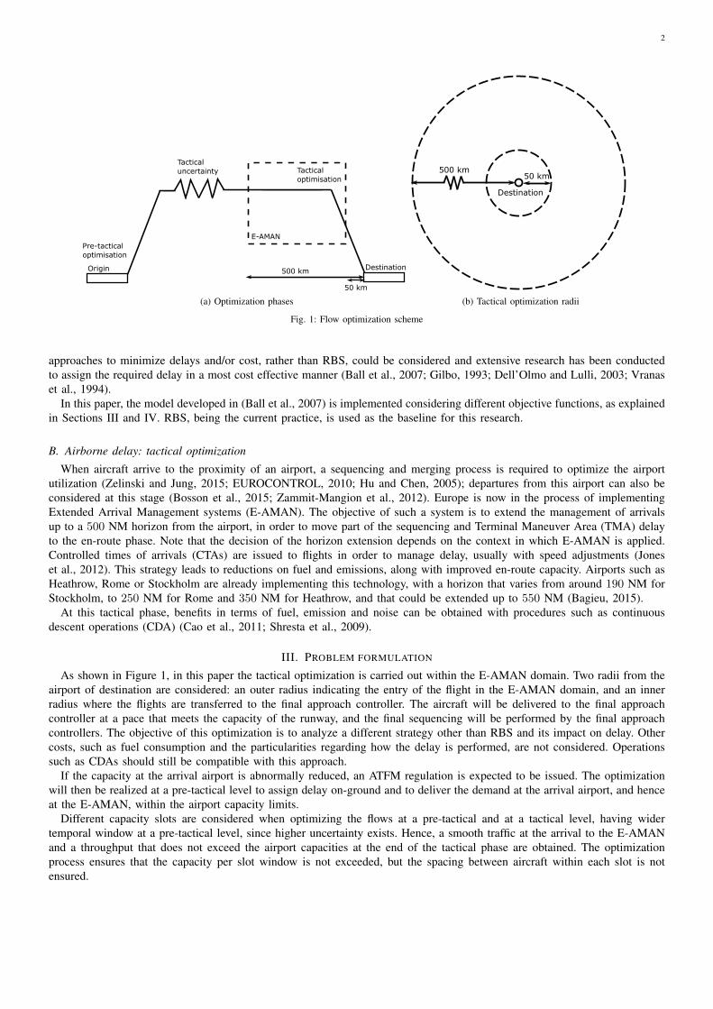
Fig. 1: Flow optimization scheme

approaches to minimize delays and/or cost, rather than RBS, could be considered and extensive research has been conductedto assign the required delay in a most cost effective manner (Ball et al., 2007; Gilbo, 1993; Dell’Olmo and Lulli, 2003; Vranaset al., 1994).

In this paper, the model developed in (Ball et al., 2007) is implemented considering different objective functions, as explainedin Sections III and IV. RBS, being the current practice, is used as the baseline for this research.

B. Airborne delay: tactical optimization

When aircraft arrive to the proximity of an airport, a sequencing and merging process is required to optimize the airportutilization (Zelinski and Jung, 2015; EUROCONTROL, 2010; Hu and Chen, 2005); departures from this airport can also beconsidered at this stage (Bosson et al., 2015; Zammit-Mangion et al., 2012). Europe is now in the process of implementingExtended Arrival Management systems (E-AMAN). The objective of such a system is to extend the management of arrivalsup to a 500 NM horizon from the airport, in order to move part of the sequencing and Terminal Maneuver Area (TMA) delayto the en-route phase. Note that the decision of the horizon extension depends on the context in which E-AMAN is applied.Controlled times of arrivals (CTAs) are issued to flights in order to manage delay, usually with speed adjustments (Joneset al., 2012). This strategy leads to reductions on fuel and emissions, along with improved en-route capacity. Airports such asHeathrow, Rome or Stockholm are already implementing this technology, with a horizon that varies from around 190 NM forStockholm, to 250 NM for Rome and 350 NM for Heathrow, and that could be extended up to 550 NM (Bagieu, 2015).

At this tactical phase, benefits in terms of fuel, emission and noise can be obtained with procedures such as continuousdescent operations (CDA) (Cao et al., 2011; Shresta et al., 2009).

III. PROBLEM FORMULATION

As shown in Figure 1, in this paper the tactical optimization is carried out within the E-AMAN domain. Two radii from theairport of destination are considered: an outer radius indicating the entry of the flight in the E-AMAN domain, and an innerradius where the flights are transferred to the final approach controller. The aircraft will be delivered to the final approachcontroller at a pace that meets the capacity of the runway, and the final sequencing will be performed by the final approachcontrollers. The objective of this optimization is to analyze a different strategy other than RBS and its impact on delay. Othercosts, such as fuel consumption and the particularities regarding how the delay is performed, are not considered. Operationssuch as CDAs should still be compatible with this approach.

If the capacity at the arrival airport is abnormally reduced, an ATFM regulation is expected to be issued. The optimizationwill then be realized at a pre-tactical level to assign delay on-ground and to deliver the demand at the arrival airport, and henceat the E-AMAN, within the airport capacity limits.

Different capacity slots are considered when optimizing the flows at a pre-tactical and at a tactical level, having widertemporal window at a pre-tactical level, since higher uncertainty exists. Hence, a smooth traffic at the arrival to the E-AMANand a throughput that does not exceed the airport capacities at the end of the tactical phase are obtained. The optimizationprocess ensures that the capacity per slot window is not exceeded, but the spacing between aircraft within each slot is notensured.

3

The maximum delay that can be assigned to a flight is also different at pre-tactical and tactical level. Here, it is consideredpossible to hold flights on-ground as long as required, so no time constraint is applied on this holding time. Note that, for specificairports where gate capacity is more limited, e.g. Logan International (Boston) and New York LaGuardia, gate capacity couldbe reached, so a time constraint should be added on the ground holding time (Wang et al., 2009; Khadilkar and Balakrishnan,2013). As for the flights within the E-AMAN domain, they are airborne and, therefore, cannot be held indefinitely.

Besides these differences, pre-tactical and tactical models follow the same formulation since the same problem is solved:assigning flights to slots. Note also that the pre-tactical optimization will be carried out once for all the flights affected bythe regulation, while the tactical optimization is a dynamic process in the sense that aircraft can be assigned different arrivaltimes each time the optimization is performed. The final arriving time is then the last one assigned before the aircraft reachesthe inner radius.

A. General ground holding problem formulation

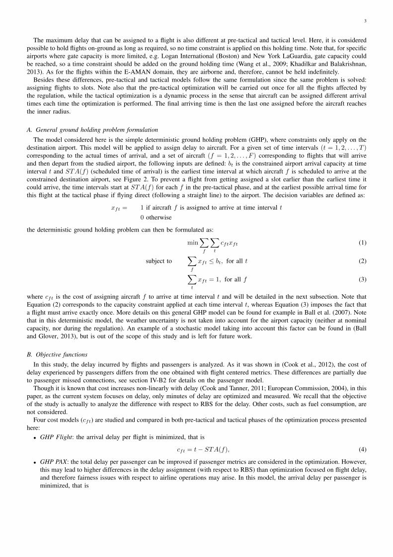
The model considered here is the simple deterministic ground holding problem (GHP), where constraints only apply on thedestination airport. This model will be applied to assign delay to aircraft. For a given set of time intervals (t = 1, 2, . . . , T )corresponding to the actual times of arrival, and a set of aircraft (f = 1, 2, . . . , F ) corresponding to flights that will arriveand then depart from the studied airport, the following inputs are defined: bt is the constrained airport arrival capacity at timeinterval t and STA(f) (scheduled time of arrival) is the earliest time interval at which aircraft f is scheduled to arrive at theconstrained destination airport, see Figure 2. To prevent a flight from getting assigned a slot earlier than the earliest time itcould arrive, the time intervals start at STA(f) for each f in the pre-tactical phase, and at the earliest possible arrival time forthis flight at the tactical phase if flying direct (following a straight line) to the airport. The decision variables are defined as:

xft = 1 if aircraft f is assigned to arrive at time interval t0 otherwise

the deterministic ground holding problem can then be formulated as:

min∑f

∑t

cftxft (1)

subject to∑f

xft ≤ bt, for all t (2)∑t

xft = 1, for all f (3)

where cft is the cost of assigning aircraft f to arrive at time interval t and will be detailed in the next subsection. Note thatEquation (2) corresponds to the capacity constraint applied at each time interval t, whereas Equation (3) imposes the fact thata flight must arrive exactly once. More details on this general GHP model can be found for example in Ball et al. (2007). Notethat in this deterministic model, the weather uncertainty is not taken into account for the airport capacity (neither at nominalcapacity, nor during the regulation). An example of a stochastic model taking into account this factor can be found in (Balland Glover, 2013), but is out of the scope of this study and is left for future work.

B. Objective functions

In this study, the delay incurred by flights and passengers is analyzed. As it was shown in (Cook et al., 2012), the cost ofdelay experienced by passengers differs from the one obtained with flight centered metrics. These differences are partially dueto passenger missed connections, see section IV-B2 for details on the passenger model.

Though it is known that cost increases non-linearly with delay (Cook and Tanner, 2011; European Commission, 2004), in thispaper, as the current system focuses on delay, only minutes of delay are optimized and measured. We recall that the objectiveof the study is actually to analyze the difference with respect to RBS for the delay. Other costs, such as fuel consumption, arenot considered.

Four cost models (cft) are studied and compared in both pre-tactical and tactical phases of the optimization process presentedhere:

• GHP Flight: the arrival delay per flight is minimized, that is

cft = t− STA(f), (4)

• GHP PAX: the total delay per passenger can be improved if passenger metrics are considered in the optimization. However,this may lead to higher differences in the delay assignment (with respect to RBS) than optimization focused on flight delay,and therefore fairness issues with respect to airline operations may arise. In this model, the arrival delay per passenger isminimized, that is

4

STA

Scheduled Time Arrival

time

STD

Scheduled Time Departure

MTT

Minimum Turnaround Time

LTA

Latest Time Arrival

Turnaround buffer:

Maximum delay

without

propagating delay

(a) Turnaround times

STA timeSTD

MTT

LTA

Actual Time Arrival

ATA

Actual Time Departure

ATD

Reactionary

delayArrival

delay

Reactionary

delay

t

(b) Delay and delay propagation

Fig. 2: Turnaround and delay diagram

cft = PAXarr(f)(t− STA(f)) (5)

where PAXarr(f) is the number of arrival passengers assigned to aircraft f , see Section IV-B2 for the details of theassignment of passengers per flight.

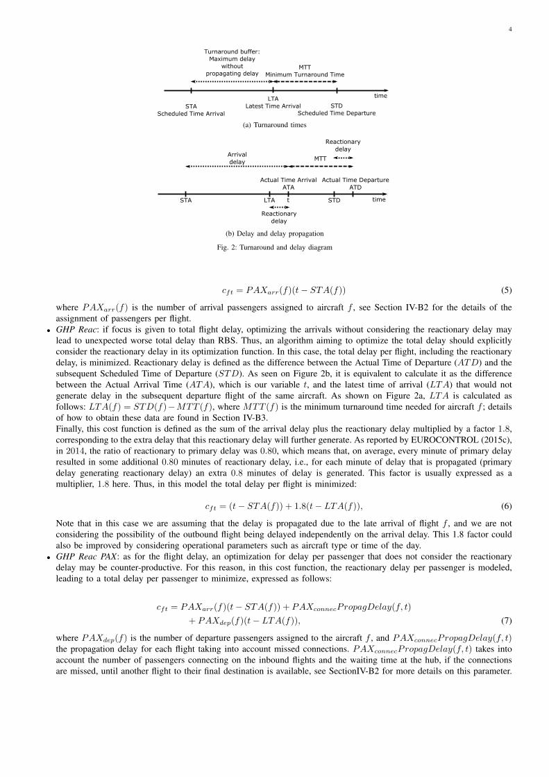
• GHP Reac: if focus is given to total flight delay, optimizing the arrivals without considering the reactionary delay maylead to unexpected worse total delay than RBS. Thus, an algorithm aiming to optimize the total delay should explicitlyconsider the reactionary delay in its optimization function. In this case, the total delay per flight, including the reactionarydelay, is minimized. Reactionary delay is defined as the difference between the Actual Time of Departure (ATD) and thesubsequent Scheduled Time of Departure (STD). As seen on Figure 2b, it is equivalent to calculate it as the differencebetween the Actual Arrival Time (ATA), which is our variable t, and the latest time of arrival (LTA) that would notgenerate delay in the subsequent departure flight of the same aircraft. As shown on Figure 2a, LTA is calculated asfollows: LTA(f) = STD(f)−MTT (f), where MTT (f) is the minimum turnaround time needed for aircraft f ; detailsof how to obtain these data are found in Section IV-B3.Finally, this cost function is defined as the sum of the arrival delay plus the reactionary delay multiplied by a factor 1.8,corresponding to the extra delay that this reactionary delay will further generate. As reported by EUROCONTROL (2015c),in 2014, the ratio of reactionary to primary delay was 0.80, which means that, on average, every minute of primary delayresulted in some additional 0.80 minutes of reactionary delay, i.e., for each minute of delay that is propagated (primarydelay generating reactionary delay) an extra 0.8 minutes of delay is generated. This factor is usually expressed as amultiplier, 1.8 here. Thus, in this model the total delay per flight is minimized:

cft = (t− STA(f)) + 1.8(t− LTA(f)), (6)

Note that in this case we are assuming that the delay is propagated due to the late arrival of flight f , and we are notconsidering the possibility of the outbound flight being delayed independently on the arrival delay. This 1.8 factor couldalso be improved by considering operational parameters such as aircraft type or time of the day.

• GHP Reac PAX: as for the flight delay, an optimization for delay per passenger that does not consider the reactionarydelay may be counter-productive. For this reason, in this cost function, the reactionary delay per passenger is modeled,leading to a total delay per passenger to minimize, expressed as follows:

cft = PAXarr(f)(t− STA(f)) + PAXconnecPropagDelay(f, t)

+ PAXdep(f)(t− LTA(f)), (7)

where PAXdep(f) is the number of departure passengers assigned to the aircraft f , and PAXconnecPropagDelay(f, t)the propagation delay for each flight taking into account missed connections. PAXconnecPropagDelay(f, t) takes intoaccount the number of passengers connecting on the inbound flights and the waiting time at the hub, if the connectionsare missed, until another flight to their final destination is available, see SectionIV-B2 for more details on this parameter.

5

IV. SCENARIO AND STOCHASTIC MODEL

A. System overview

Figure 1 presents the overview of the systems modeled in this paper. The tactical optimization can be carried out with orwithout a pre-tactical optimization. The pre-tactical phase will be required when the airport capacity is abnormally reduced. Inthat case, controlled time of departures (CTD) will be issued to the flights, which should take off within a 15-minutes window,i.e., between 10 minutes before and 5 minutes around this CTD. As shown in (Tielrooij et al., 2015), the actual time whenthe aircraft will arrive at the airport once departed is subject to variability as the flight is affected by factors, such as weather,tactical flow management by air traffic control and direct routes. In Figure 1a, this is represented as tactical uncertainty onthe demand.

Three different flights datasets are considered: the original demand, the controlled demand, where on-ground delay has beenissued at a pre-tactical phase, and the tactical demand, where flights will be considered when arriving at the domain of theE-AMAN.

1) Pre-tactical phase model: The first phase of the optimization process consists in solving the problem in the pre-tacticalphase, in a static process. Slots t are typically considered of 15 minute-length. Note that here, and throughout the paper, slotsare considered as time bins that can hold several flights (up to the corresponding maximum capacity for this time bin). Theseslots are wide enough to ensure a smooth traffic at the arrival to the E-AMAN and a throughput that does not exceed the airportcapacities at the end of the tactical phase. The optimization process is applied considering the STAs and airport capacity asinputs, and obtaining a regulated demand.

2) Tactical phase model: Tactical uncertainty is added to the regulated demand in order to obtain the actual arrival demandto the airport, see Section IV-C for more details on this uncertainty addition.

In the tactical phase, the optimization that would be performed by the controllers at the E-AMAN, within the inner andouter radii, is modeled. The airspace considered is located around the airport within two radius, outer and inner. In our casestudy, radii of 500 km and 50 km are considered (270 NM to 27 NM), the center of these radii being the arrival airport, seeFigure 1b. In this airspace, traffic will arrive according to the actual demand and a dynamic optimization is carried out so thattraffic reaches the inner radius within slot windows t of 3 minute-width, and is thus metered within these slots to the finalapproach controller. The optimization process maintains the capacity per slot window without exceeding its capacity. However,even if the flow is smoothed, the spacing between aircraft within each slot is not ensured. The final spacing and metering,before landing, is assumed to be carried out by the final approach controller, once the aircraft is within the inner radius.

Every time an aircraft enters this airspace (outer radius), the delay assignment optimization is solved for a distinct problem.The earliest arrival times at the inner radius of all flights within the considered airspace are computed and an optimization isrealized. The earliest arrival time is computed assuming that the aircraft could fly a straight trajectory toward the destinationairport from its estimated current position, which is in line with ATCO practices of giving direct instructions and pilotsrequesting these trajectories (Delgado, 2015), even though, from an operational point of view, this is an ideal trajectory. Butonce again, the objective in this study is to compute the best possible outcomes of the different optimization models in orderto quantify if further research to incorporate these optimizations at operational level should be realized. Note that, in somecases, this earliest arrival time may be earlier than the original intended scheduled arrival time, leading to negative tacticaldelay.

This is a dynamic process in the sense that an aircraft can be assigned different arrival times each time the optimization isperformed. The final arriving time is the last one assigned before the aircraft reaches the inner radius. When a RBS policy isapplied instead of the optimization, once the aircraft enters the E-AMAN horizon, a slot is given and this assignment is notchanged anymore.

In this case, the delay will not be performed on-ground but as holding, path stretching and/or speed adjustments within theE-AMAN domain airspace. Commission Regulation (EU) No 965/2012, which lays down requirements related to air operationsand the acceptable means of compliance and guidance material on fuel policy, specifies that an aircraft operator shall ensurethat flights operate with a final reserve fuel of 30 minutes at holding speed at 1500 ft above the aerodrome elevation in standardconditions (European Commission, 2012; EASA, 2017). Considering that the delay assigned at the E-AMAN can be absorbedwhile approaching the airport and not just by holding, the maximum delay considered to be assigned to an individual flight isset to 35 minutes.

B. Scenario

As summarized in Table I, a scenario in our model is formed by a set of parameters defining the:• airport capacity, see Section IV-B1;• traffic demand, scheduled departure, arrival and following departure times, see Section IV-B1;• passengers demand to individual flights, see Section IV-B2;• waiting time for further flights to final destination for passengers with missed connections, see Section IV-B2;• scheduled and minimum time required for turnaround, see IV-B3;• tactical inner and outer radii distances;

6

TABLE I: Scenario and stochastic parameters

Model part Model sub-part Description Times generated

Scenario

Traffic demand

• Based on 12SEP14 CDG arrivals• Between 5:00 and 11:00 GMT• Canceled flights considered pre-tactically but not tactically• Flight within inner radius excluded

Once

Turnaround

• AC type for turn around• AC types top 10 used• AC category otherwise• Burr and Weibull distribution fitting• MTT (f) = max(rand(0.1, 0.4), STT (f))

Passenger demand • Triangular distribution between 60%-95% centered at 85%• Connections modeled based on analysis of day of operations

Capacity • 80 acc/h nominal• 40 acc/h regulated

Radii • Outer 500 km (270 NM)• Inner 50 km (27 NM)

Optimization slot width • 15’ pre-tactical (20acc/15’ nominal, 10acc/15’ regulated)• 3’ tactical (4acc/3’ nominal, 2acc/3’ regulated)

Tactical noise • Difference between controlled and actual arrival times• Burr distribution

Monte Carlo200 times

• pre-tactical and tactical optimization slot width.All previous parameters are estimated once to generate the scenario for the optimization models. Then, tactical uncertainty

is applied 200 times on this scenario, in a Monte Carlo simulation, generating results that do not depend on a particular tacticaluncertainty.

Both in pre-tactical and tactical optimizations, the GHP objective functions presented in Section III-B are compared to aRBS formulation.

1) Traffic demand and capacity: The demand at Paris CDG airport on September 12th, 2014 has been considered for thesimulations; it was a busy Friday without any major disruption. The morning traffic, between 5.00 GMT and 11.00 GMT,is analyzed. For the traffic scheduled, data from EUROCONTROL Demand Data Repository 2 (DDR2) (EUROCONTROL,2015b) have been used. Note that these data represent the filed flight plans and might differ from the actual schedules, but arethe final flights plans and hence the final demand.

During these 6 hours of study, the total number of aircraft scheduled to arrive at CDG is 285. 12 flights that were consideredin the demand at the pre-tactical phase were canceled, so they are not included in the tactical phase. The final number offlights actually considered in the tactical phase is thus 273. Note that in the case of having flights taking off within the innerradius or realizing a circular flight (which corresponds to an extremely low number of flights for a hub airport), they will bemanaged by the final approach controllers on their sequencing, and assigned the first available slot depending on their ETA.Finally, the hypothesis that every arriving aircraft will eventually depart is made.

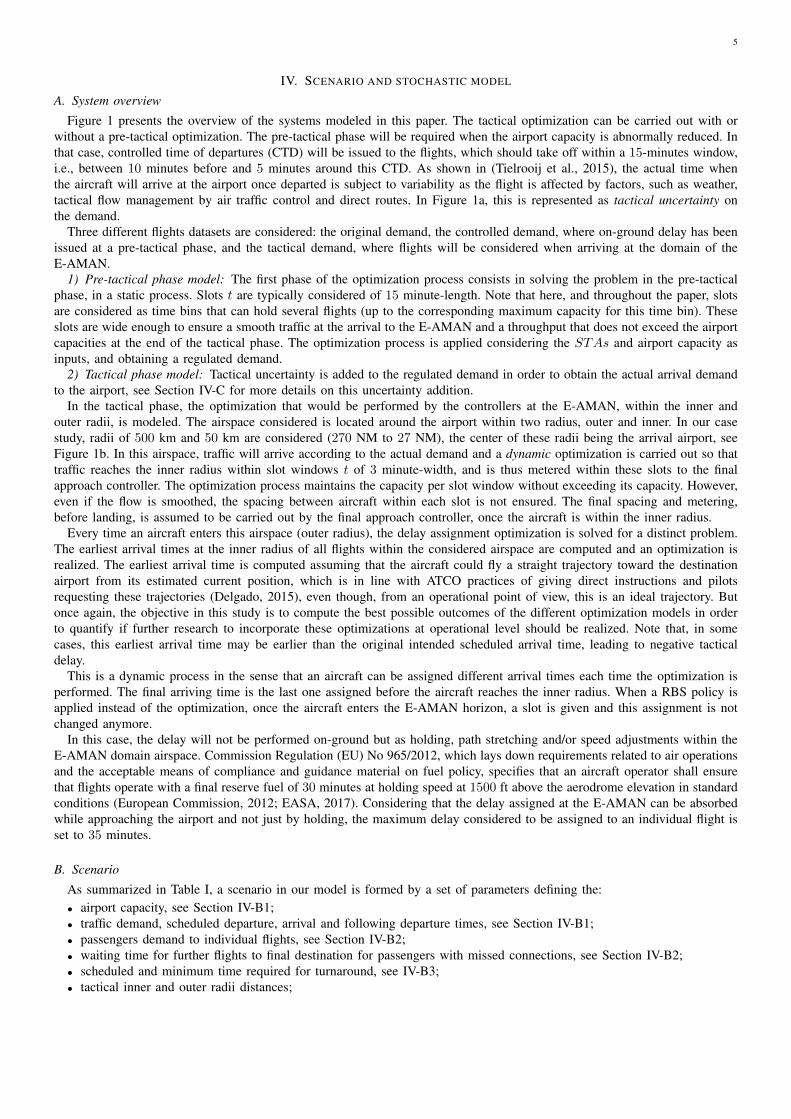
Considering the demand data and historic regulations at CDG, an ATFM regulation between 6.00 GMT and 8.00 GMT ismodeled. A nominal capacity of 80 arrivals per hour is considered when no regulation is applied, ensuring that the pre-tacticaloptimization does not affect the demand, and the regulated capacity is set to 40, which is a possible value of capacity duringregulated periods at CGC as shown in the DDR2 dataset (EUROCONTROL, 2015b). These capacity values have been comparedto the traffic demand, as seen in Figure 3, to ensure these are reasonable values.

For the optimization, slot windows of 15 minutes are considered in the pre-tactical phase, i.e., 20 (nominal) or 10 (regulated)aircraft every 15 minutes, and of 3 minutes in the tactical one, i.e., 4 or 2 aircraft every 3 minutes.

2) Passenger model: For each flight, the type of aircraft has been considered and the number of passengers in each flight hasbeen estimated as a function of the maximum capacity of the aircraft. Air France reported an overall load factor of 84.7% for2014 (Air France-KLM, 2015), the Association of European Airlines reported an average load factor of 83.6% for September2014 (Association of European Airlines, 2015) and Aeroport de Paris a seat load factor of 83.4% for Paris-CDG and Paris-ORYairports (Aeroports de Paris, 2014). Considering these reported load factors, the target average load factor has been defined as85%. However, individual load factors vary from having almost full flights to flights with a low occupancy. For this reason, atriangular distribution has been used to allocate passengers between 60 and 95% of the maximum capacity, with the peak ofthe distribution at 85%, which is considered as the target average load factor. Note that, if data were available, a more detailedstatistical model could be used. The triangular distribution is the simplest one allowing us to generate individual variations onthe load factors within the flights, being bounded, and with a mean load factor meeting the average reported load factor atoperations at the airport.

The propagation of passenger delay, due to missed connections at the hub, has been modeled by simulating the number ofpassengers connecting on the inbound flights and the waiting time at the hub, if the connections are missed, until another flightto their final destination is available. For each airline, the probability of having connecting passengers on each of their flightand how many passengers connecting has been estimated. These probabilities have been used to assign, or not, connectingpassengers to a given inbound flight. Inbound connecting passengers in a given flight are grouped considering their connecting

7

0500 0600 0700 0800 0900 1000 11000

10

20

30

40

50

60

70

80

Nu

mb

er

of

arr

ivin

g f

ligh

ts

GMT time

Arrival demand at CDG, 12 Sept 2014

Fig. 3: Arrival demand at CDG (12 Sep 2014) with capacity

0 200 400 600 800 1000 1200 1400 1600

Arrival delay inbound flight (min)

0

500

1000

1500

Pro

pagate

ddela

y,extr

aw

aitin

gtim

e(m

in)

planned

connection

missing

connectionwaiting

1st possibility

missing

connectionwaiting

2nd possibility

missing

connectionwaiting

3rd possibility

missing

connectionwaiting

next day

(a) One passenger connecting

0 200 400 600 800 1000 1200 1400 1600

Arrival delay inbound flight (min)

0

5000

10000

15000P

ropagate

d d

ela

y, extr

a w

aitin

g tim

e (

min

)

(b) Several passengers connecting

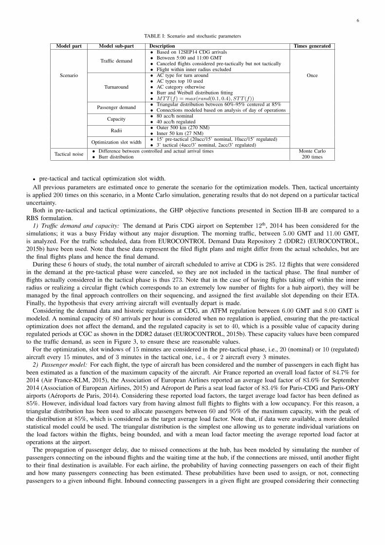
Fig. 4: Example of extra delay due to missed connections

outbound flight creating groups of passengers traveling together. For each of these connecting groups of passengers, and basedon probabilities obtained from the analysis of itineraries modeling one day of operations, their waiting time for their firstconnection and their minimum connecting time (depending on the probability of being connecting to national or internationalflights) has been estimated. If the connection is missed due to a delay in the inbound flight, the waiting time for a nextflight to the same destination and airline has been estimated for forthcoming departures from the hub. The estimations ofpassengers groups and connectivity are based on the statistical analysis of a day of itineraries at the hub from individualpassengers’ itineraries developed in SESAR WP-E ComplexityCost project (Cook et al., 2016; Delgado et al., 2016a; SESARJoint Undertaking, 2016) and analyzing the flights on the day. Using this methodology, in this research, instead of individualitineraries, the number of connecting passengers and their waiting times are modeled and approximated to realistic operationsat the hub.

This passenger allocation process leads to a total of 39, 820 arrival passengers, from which 8, 620 are connecting to followingflights (21.6% of arrival passengers) and a total of 39, 671 departure passengers, during the 6-hour study. The number ofconnections modeled is in line with the values reported by Aeroports de Paris September 2014 statistics (19.3% of connectingpassengers considering both Paris-CDG and Paris-ORY) (Aeroports de Paris, 2014).

Figure 4 shows two examples of propagation of delay for two inbound flights in the hub. In Figure 4a, an inbound flightwith one single connecting passenger is presented. In this case, the passenger connection flight leaves 220 minutes after thearrival of the inbound and there is a minimum connecting time of 107 minutes. Therefore, if the inbound is delayed by morethan 113 minutes, the connection is missed and the passenger will incur an extra 265 minutes of delay (missing connectionwaiting for 1st possibility in Figure 4a). Note that from that time on, if the inbound flight is further delayed, the waiting timefor the next available outbound flight decreases; this ensures that the total passenger delay does not double count the arrival

8

A320 A319 A321 A318 B77W B738 A332 B772 RJ85 B7630

200

400

600

800

1000

1200

1400

1600

1800

2000

Nu

mb

er

of

flig

hts

Type of aircraft

0%

10%

19%

29%

39%

48%

58%

68%

77%

87%

97%

Fig. 5: Classification of flights depending on aircraft type

0 50 100 150 200 250 300 350 4000

0.1

0.2

0.3

0.4

0.5

0.6

0.7

0.8

0.9

1

T: Turnaround time [min]

Pro

po

rtio

n u

ntil T

Burr probability distribution

Real data

Fig. 6: Probability distribution of A320 turnaround time

and waiting delay: an extra minute of delay on arrival means a minute less waiting for the following outbound. However, ifthe inbound flight is delayed more than 379 minutes the second flight to the final destination is also missed and 510 moreminutes need to be waited to the next available connection (missing connection waiting for 2nd possibility in Figure 4a).Figure 4b shows another example where 13 inbound passengers are connecting with different flights and each one of themwith different further connection options. Note that the waiting delay is the aggregated delay for all the passengers missingtheir connections, obtaining in this manner the total extra delay propagated for the passengers, and that it corresponds to theparameter PAXconnecPropagDelay(f, t) in Equation (7).

3) Turnaround model: As previously commented, some arriving flights delayed at the airport might propagate this delayto their subsequent departure (reactionary delay). To be able to model this propagation effect, the scheduled turnaround times(STT) and the minimum time required to do the turnaround process (MTT) have been computed for each flight.

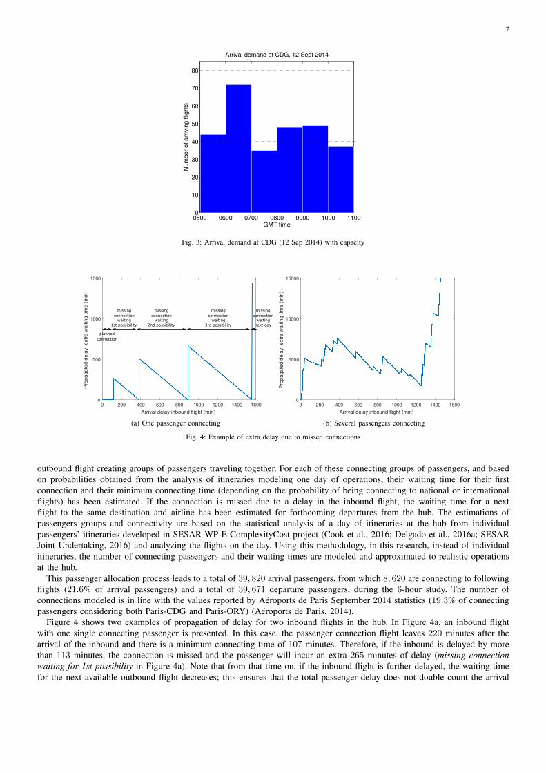
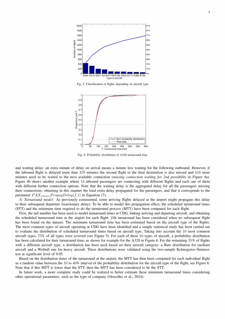
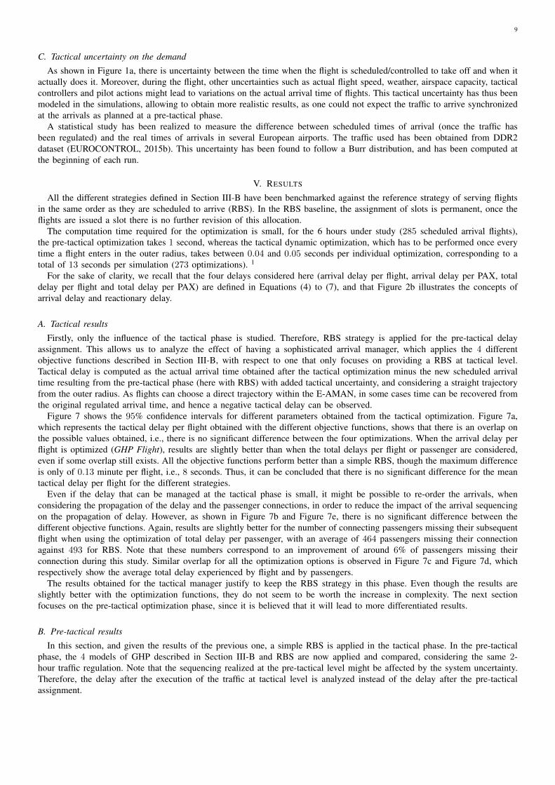
First, the tail number has been used to model turnaround times at CDG, linking arriving and departing aircraft, and obtainingthe scheduled turnaround time at the airport for each flight. 24h turnaround has been considered when no subsequent flighthas been found on the dataset. The minimum turnaround time has been estimated based on the aircraft type of the flights.The most common types of aircraft operating at CDG have been identified and a simple statistical study has been carried outto evaluate the distribution of scheduled turnaround times based on aircraft type. Taking into account the 10 most commonaircraft types, 75% of all types were covered (see Figure 5). For each of these 10 types of aircraft, a probability distributionhas been calculated for their turnaround time, as shown for example for the A320 in Figure 6. For the remaining 25% of flightswith a different aircraft type, a distribution has been used based on their aircraft category: a Burr distribution for mediumaircraft and a Weibull one for heavy aircraft. These distributions were validated using the two-sample Kolmogorov-Smirnovtest at significant level of 0.05.

Based on the distribution times of the turnaround at the airport, the MTT has then been computed for each individual flightas a random value between the 10 to 40% interval of the probability distribution for the aircraft type of the flight, see Figure 6.Note that if this MTT is lower than the STT, then the MTT has been considered to be the STT.

In future work, a more complete study could be realized to better estimate these minimum turnaround times consideringother operational parameters, such as the type of company (Oreschko et al., 2014).

9

C. Tactical uncertainty on the demand

As shown in Figure 1a, there is uncertainty between the time when the flight is scheduled/controlled to take off and when itactually does it. Moreover, during the flight, other uncertainties such as actual flight speed, weather, airspace capacity, tacticalcontrollers and pilot actions might lead to variations on the actual arrival time of flights. This tactical uncertainty has thus beenmodeled in the simulations, allowing to obtain more realistic results, as one could not expect the traffic to arrive synchronizedat the arrivals as planned at a pre-tactical phase.

A statistical study has been realized to measure the difference between scheduled times of arrival (once the traffic hasbeen regulated) and the real times of arrivals in several European airports. The traffic used has been obtained from DDR2dataset (EUROCONTROL, 2015b). This uncertainty has been found to follow a Burr distribution, and has been computed atthe beginning of each run.

V. RESULTS

All the different strategies defined in Section III-B have been benchmarked against the reference strategy of serving flightsin the same order as they are scheduled to arrive (RBS). In the RBS baseline, the assignment of slots is permanent, once theflights are issued a slot there is no further revision of this allocation.

The computation time required for the optimization is small, for the 6 hours under study (285 scheduled arrival flights),the pre-tactical optimization takes 1 second, whereas the tactical dynamic optimization, which has to be performed once everytime a flight enters in the outer radius, takes between 0.04 and 0.05 seconds per individual optimization, corresponding to atotal of 13 seconds per simulation (273 optimizations). 1

For the sake of clarity, we recall that the four delays considered here (arrival delay per flight, arrival delay per PAX, totaldelay per flight and total delay per PAX) are defined in Equations (4) to (7), and that Figure 2b illustrates the concepts ofarrival delay and reactionary delay.

A. Tactical results

Firstly, only the influence of the tactical phase is studied. Therefore, RBS strategy is applied for the pre-tactical delayassignment. This allows us to analyze the effect of having a sophisticated arrival manager, which applies the 4 differentobjective functions described in Section III-B, with respect to one that only focuses on providing a RBS at tactical level.Tactical delay is computed as the actual arrival time obtained after the tactical optimization minus the new scheduled arrivaltime resulting from the pre-tactical phase (here with RBS) with added tactical uncertainty, and considering a straight trajectoryfrom the outer radius. As flights can choose a direct trajectory within the E-AMAN, in some cases time can be recovered fromthe original regulated arrival time, and hence a negative tactical delay can be observed.

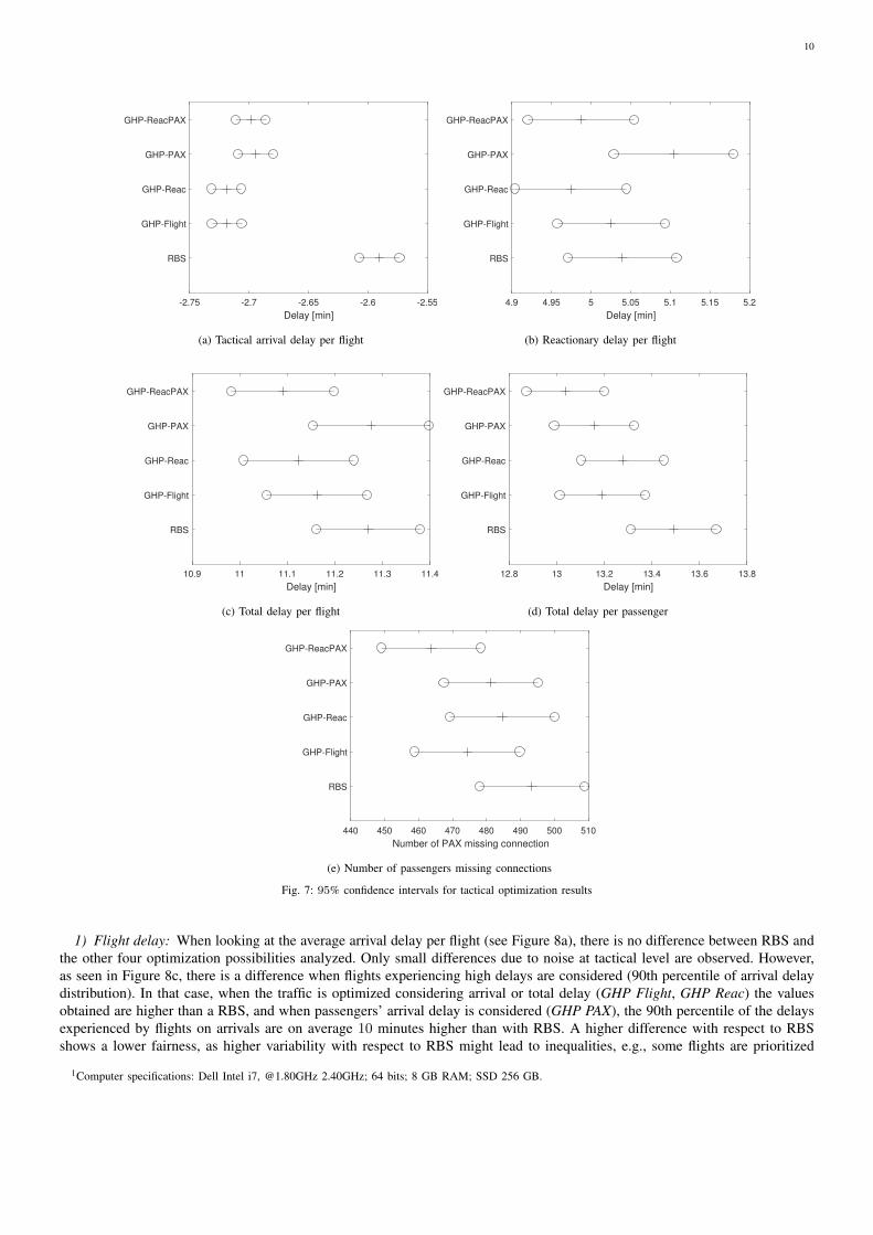
Figure 7 shows the 95% confidence intervals for different parameters obtained from the tactical optimization. Figure 7a,which represents the tactical delay per flight obtained with the different objective functions, shows that there is an overlap onthe possible values obtained, i.e., there is no significant difference between the four optimizations. When the arrival delay perflight is optimized (GHP Flight), results are slightly better than when the total delays per flight or passenger are considered,even if some overlap still exists. All the objective functions perform better than a simple RBS, though the maximum differenceis only of 0.13 minute per flight, i.e., 8 seconds. Thus, it can be concluded that there is no significant difference for the meantactical delay per flight for the different strategies.

Even if the delay that can be managed at the tactical phase is small, it might be possible to re-order the arrivals, whenconsidering the propagation of the delay and the passenger connections, in order to reduce the impact of the arrival sequencingon the propagation of delay. However, as shown in Figure 7b and Figure 7e, there is no significant difference between thedifferent objective functions. Again, results are slightly better for the number of connecting passengers missing their subsequentflight when using the optimization of total delay per passenger, with an average of 464 passengers missing their connectionagainst 493 for RBS. Note that these numbers correspond to an improvement of around 6% of passengers missing theirconnection during this study. Similar overlap for all the optimization options is observed in Figure 7c and Figure 7d, whichrespectively show the average total delay experienced by flight and by passengers.

The results obtained for the tactical manager justify to keep the RBS strategy in this phase. Even though the results areslightly better with the optimization functions, they do not seem to be worth the increase in complexity. The next sectionfocuses on the pre-tactical optimization phase, since it is believed that it will lead to more differentiated results.

B. Pre-tactical results

In this section, and given the results of the previous one, a simple RBS is applied in the tactical phase. In the pre-tacticalphase, the 4 models of GHP described in Section III-B and RBS are now applied and compared, considering the same 2-hour traffic regulation. Note that the sequencing realized at the pre-tactical level might be affected by the system uncertainty.Therefore, the delay after the execution of the traffic at tactical level is analyzed instead of the delay after the pre-tacticalassignment.

10

-2.75 -2.7 -2.65 -2.6 -2.55

Delay [min]

RBS

GHP-Flight

GHP-Reac

GHP-PAX

GHP-ReacPAX

(a) Tactical arrival delay per flight

4.9 4.95 5 5.05 5.1 5.15 5.2

Delay [min]

RBS

GHP-Flight

GHP-Reac

GHP-PAX

GHP-ReacPAX

(b) Reactionary delay per flight

10.9 11 11.1 11.2 11.3 11.4

Delay [min]

RBS

GHP-Flight

GHP-Reac

GHP-PAX

GHP-ReacPAX

(c) Total delay per flight

12.8 13 13.2 13.4 13.6 13.8

Delay [min]

RBS

GHP-Flight

GHP-Reac

GHP-PAX

GHP-ReacPAX

(d) Total delay per passenger

440 450 460 470 480 490 500 510

Number of PAX missing connection

RBS

GHP-Flight

GHP-Reac

GHP-PAX

GHP-ReacPAX

(e) Number of passengers missing connections

Fig. 7: 95% confidence intervals for tactical optimization results

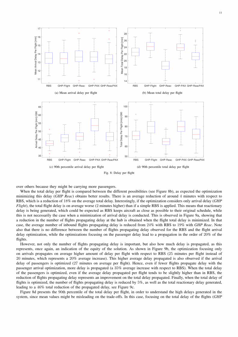
1) Flight delay: When looking at the average arrival delay per flight (see Figure 8a), there is no difference between RBS andthe other four optimization possibilities analyzed. Only small differences due to noise at tactical level are observed. However,as seen in Figure 8c, there is a difference when flights experiencing high delays are considered (90th percentile of arrival delaydistribution). In that case, when the traffic is optimized considering arrival or total delay (GHP Flight, GHP Reac) the valuesobtained are higher than a RBS, and when passengers’ arrival delay is considered (GHP PAX), the 90th percentile of the delaysexperienced by flights on arrivals are on average 10 minutes higher than with RBS. A higher difference with respect to RBSshows a lower fairness, as higher variability with respect to RBS might lead to inequalities, e.g., some flights are prioritized

1Computer specifications: Dell Intel i7, @1.80GHz 2.40GHz; 64 bits; 8 GB RAM; SSD 256 GB.

11

RBS GHP-Flight GHP-Reac GHP-PAX GHP-ReacPAX

11

12

13

14

15

16

17

Me

an

Arr

iva

l D

ela

y P

er

Flig

ht

[min

]

(a) Mean arrival delay per flight


14

16

18

20

22

24

26

28

Me

an

To

tal D

ela

y P

er

Flig

ht

[min

]

(b) Mean total delay per flight


35

40

45

50

55

60

65

Arr

iva

l D

ela

y P

er

Flig

ht

[min

]-Q

90

(c) 90th percentile arrival delay per flight


50

60

70

80

90

100

To

tal D

ela

y P

er

Flig

ht

[min

]-Q

90

(d) 90th percentile total delay per flight

Fig. 8: Delay per flight

over others because they might be carrying more passengers.When the total delay per flight is compared between the different possibilities (see Figure 8b), as expected the optimization

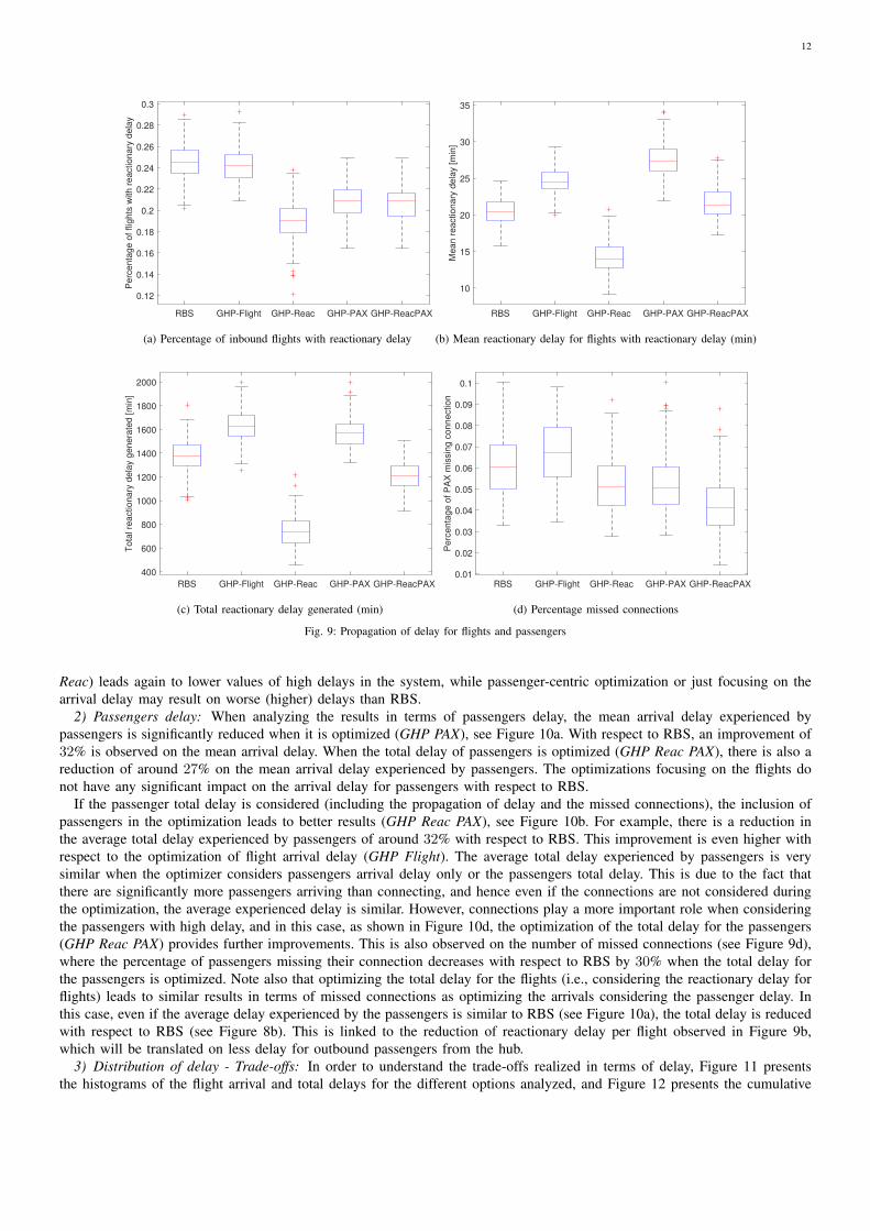
minimizing this delay (GHP Reac) obtains better results. There is an average reduction of around 4 minutes with respect toRBS, which is a reduction of 18% on the average total delay. Interestingly, if the optimization considers only arrival delay (GHPFlight), the total flight delay is on average worse (2 minutes higher) than if a simple RBS is applied. This means that reactionarydelay is being generated, which could be expected as RBS keeps aircraft as close as possible to their original schedule, whilethis is not necessarily the case when a minimization of arrival delay is conducted. This is observed in Figure 9a, showing thata reduction in the number of flights propagating delay at the hub is obtained when the flight total delay is minimized. In thatcase, the average number of inbound flights propagating delay is reduced from 24% with RBS to 19% with GHP Reac. Notealso that there is no difference between the number of flights propagating delay observed for the RBS and the flight arrivaldelay optimization, while the optimizations focusing on the passenger delay lead to a propagation in the order of 20% of theflights.

However, not only the number of flights propagating delay is important, but also how much delay is propagated, as thisrepresents, once again, an indication of the equity of the solution. As shown in Figure 9b, the optimization focusing onlyon arrivals propagates on average higher amount of delay per flight with respect to RBS (25 minutes per flight instead of20 minutes, which represents a 20% average increase). This higher average delay propagated is also observed if the arrivaldelay of passengers is optimized (27 minutes on average per flight). Hence, even if fewer flights propagate delay with thepassenger arrival optimization, more delay is propagated (a 35% average increase with respect to RBS). When the total delayof the passengers is optimized, even if the average delay propagated per flight tends to be slightly higher than in RBS, thereduction of flights propagating delay represents an improvement on the total delay propagated. Finally, when the total delay offlights is optimized, the number of flights propagating delay is reduced by 5%, as well as the total reactionary delay generated,leading to a 46% total reduction of the propagated delay, see Figure 9c.

Figure 8d presents the 90th percentile of the total delay per flight, in order to understand the high delays generated in thesystem, since mean values might be misleading on the trade-offs. In this case, focusing on the total delay of the flights (GHP

12


0.12

0.14

0.16

0.18

0.2

0.22

0.24

0.26

0.28

0.3

Pe

rce

nta

ge

of

flig

hts

with

re

actio

na

ry d

ela

y

(a) Percentage of inbound flights with reactionary delay


10

15

20

25

30

35

Me

an

re

actio

na

ry d

ela

y [

min

]

(b) Mean reactionary delay for flights with reactionary delay (min)


400

600

800

1000

1200

1400

1600

1800

2000

To

tal re

actio

na

ry d

ela

y g

en

era

ted

[m

in]

(c) Total reactionary delay generated (min)

RBS GHP-Flight GHP-Reac GHP-PAX GHP-ReacPAX0.01

0.02

0.03

0.04

0.05

0.06

0.07

0.08

0.09

0.1

Pe

rce

nta

ge

of

PA

X m

issin

g c

on

ne

ctio

n

(d) Percentage missed connections

Fig. 9: Propagation of delay for flights and passengers

Reac) leads again to lower values of high delays in the system, while passenger-centric optimization or just focusing on thearrival delay may result on worse (higher) delays than RBS.

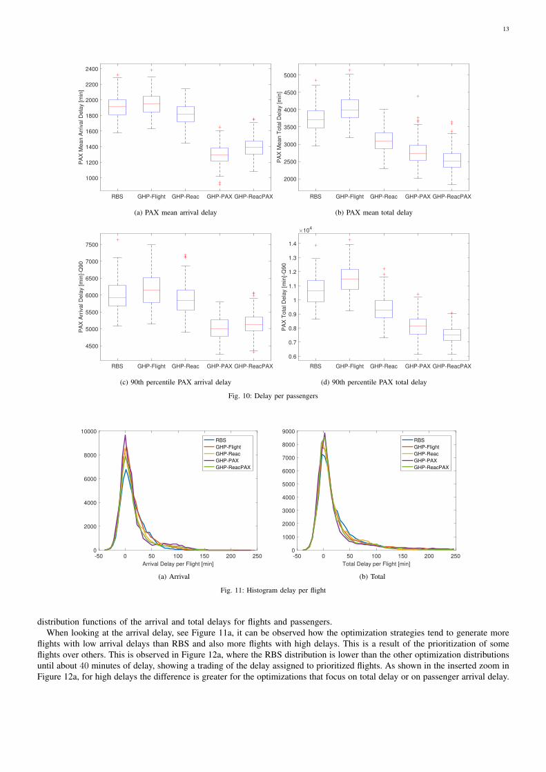
2) Passengers delay: When analyzing the results in terms of passengers delay, the mean arrival delay experienced bypassengers is significantly reduced when it is optimized (GHP PAX), see Figure 10a. With respect to RBS, an improvement of32% is observed on the mean arrival delay. When the total delay of passengers is optimized (GHP Reac PAX), there is also areduction of around 27% on the mean arrival delay experienced by passengers. The optimizations focusing on the flights donot have any significant impact on the arrival delay for passengers with respect to RBS.

If the passenger total delay is considered (including the propagation of delay and the missed connections), the inclusion ofpassengers in the optimization leads to better results (GHP Reac PAX), see Figure 10b. For example, there is a reduction inthe average total delay experienced by passengers of around 32% with respect to RBS. This improvement is even higher withrespect to the optimization of flight arrival delay (GHP Flight). The average total delay experienced by passengers is verysimilar when the optimizer considers passengers arrival delay only or the passengers total delay. This is due to the fact thatthere are significantly more passengers arriving than connecting, and hence even if the connections are not considered duringthe optimization, the average experienced delay is similar. However, connections play a more important role when consideringthe passengers with high delay, and in this case, as shown in Figure 10d, the optimization of the total delay for the passengers(GHP Reac PAX) provides further improvements. This is also observed on the number of missed connections (see Figure 9d),where the percentage of passengers missing their connection decreases with respect to RBS by 30% when the total delay forthe passengers is optimized. Note also that optimizing the total delay for the flights (i.e., considering the reactionary delay forflights) leads to similar results in terms of missed connections as optimizing the arrivals considering the passenger delay. Inthis case, even if the average delay experienced by the passengers is similar to RBS (see Figure 10a), the total delay is reducedwith respect to RBS (see Figure 8b). This is linked to the reduction of reactionary delay per flight observed in Figure 9b,which will be translated on less delay for outbound passengers from the hub.

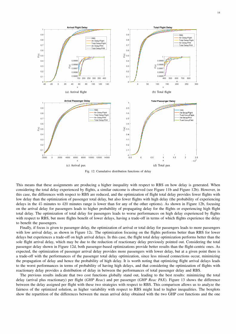
3) Distribution of delay - Trade-offs: In order to understand the trade-offs realized in terms of delay, Figure 11 presentsthe histograms of the flight arrival and total delays for the different options analyzed, and Figure 12 presents the cumulative

13


1000

1200

1400

1600

1800

2000

2200

2400

PA

X M

ea

n A

rriv

al D

ela

y [

min

]

(a) PAX mean arrival delay


2000

2500

3000

3500

4000

4500

5000

PA

X M

ea

n T

ota

l D

ela

y [

min

]

(b) PAX mean total delay


4500

5000

5500

6000

6500

7000

7500

PA

X A

rriv

al D

ela

y [

min

]-Q

90

(c) 90th percentile PAX arrival delay


0.6

0.7

0.8

0.9

1

1.1

1.2

1.3

1.4

PA

X T

ota

l D

ela

y [

min

]-Q

90

104

(d) 90th percentile PAX total delay

Fig. 10: Delay per passengers

-50 0 50 100 150 200 250

Arrival Delay per Flight [min]

0

2000

4000

6000

8000

10000

RBS

GHP-Flight

GHP-Reac

GHP-PAX

GHP-ReacPAX

(a) Arrival

-50 0 50 100 150 200 250

Total Delay per Flight [min]

0

1000

2000

3000

4000

5000

6000

7000

8000

9000

RBS

GHP-Flight

GHP-Reac

GHP-PAX

GHP-ReacPAX

(b) Total

Fig. 11: Histogram delay per flight

distribution functions of the arrival and total delays for flights and passengers.When looking at the arrival delay, see Figure 11a, it can be observed how the optimization strategies tend to generate more

flights with low arrival delays than RBS and also more flights with high delays. This is a result of the prioritization of someflights over others. This is observed in Figure 12a, where the RBS distribution is lower than the other optimization distributionsuntil about 40 minutes of delay, showing a trading of the delay assigned to prioritized flights. As shown in the inserted zoom inFigure 12a, for high delays the difference is greater for the optimizations that focus on total delay or on passenger arrival delay.

14

-40 -20 0 20 40 60 80 100 120 140

x

0

0.1

0.2

0.3

0.4

0.5

0.6

0.7

0.8

0.9

1

F(x

)

Arrival Flight Delay

RBS

Arr Delay/Flight

Total Delay/Flight

Arr Delay/PAX

Total Delay/PAX

150 200 250 300 350 400

x

0.9995

0.9996

0.9997

0.9998

0.9999

1

F(x

)

(a) Arrival flight

0 50 100 150 200 250 300

x

0

0.1

0.2

0.3

0.4

0.5

0.6

0.7

0.8

0.9

1

F(x

)

Total Flight Delay

RBS

Arr Delay/Flight

Total Delay/Flight

Arr Delay/PAX

Total Delay/PAX

400 500 600 700 800

x

0.9995

0.9996

0.9997

0.9998

0.9999

1

F(x

)

(b) Total flight

-2000 0 2000 4000 6000 8000 10000 12000 14000

x

0

0.1

0.2

0.3

0.4

0.5

0.6

0.7

0.8

0.9

1

F(x

)

Arrival Passenger Delay

RBS

Arr Delay/Flight

Total Delay/Flight

Arr Delay/PAX

Total Delay/PAX

(c) Arrival pax (d) Total pax

Fig. 12: Cumulative distribution functions of delay

This means that these assignments are producing a higher inequality with respect to RBS on how delay is generated. Whenconsidering the total delay experienced by flights, a similar outcome is observed (see Figure 11b and Figure 12b). However, inthis case, the differences with respect to RBS are reduced, and the optimization of flight total delay provides fewer flights withlow delay than the optimization of passenger total delay, but also fewer flights with high delay (the probability of experiencingdelays in the 45 minutes to 420 minutes range is lower than for any of the other options). As shown in Figure 12b, focusingon the arrival delay for passengers leads to higher probability of propagating delay for the flights or experiencing high flighttotal delay. The optimization of total delay for passengers leads to worse performances on high delay experienced by flightswith respect to RBS, but more flights benefit of lower delays, having a trade-off in terms of which flights experience the delayto benefit the passengers.

Finally, if focus is given to passenger delay, the optimization of arrival or total delay for passengers leads to more passengerswith low arrival delay, as shown in Figure 12c. The optimization focusing on the flights performs better than RBS for lowerdelays but experiences a trade-off on high arrival delays. In this case, the flight total delay optimization performs better than thesole flight arrival delay, which may be due to the reduction of reactionary delay previously pointed out. Considering the totalpassenger delay shown in Figure 12d, both passenger-based optimizations provide better results than the flight-centric ones. Asexpected, the optimization of passenger arrival delay provides more passengers with lower delay, but at a given point there isa trade-off with the performances of the passenger total delay optimization, since less missed connections occur, minimizingthe propagation of delay and hence the probability of high delay. It is worth noting that optimizing flight arrival delays leadsto the worst performances in terms of probability of having high delays, and that considering the optimization of flights withreactionary delay provides a distribution of delay in between the performances of total passenger delay and RBS.

The previous results indicate that two cost functions globally stand out, leading to the best results: minimizing the totaldelay (arrival plus reactionary) per flight (GHP Reac) and per passenger (GHP Reac PAX). Figure 13 shows the differencebetween the delay assigned per flight with these two strategies with respect to RBS. This comparison allows us to analyze thefairness of the optimized solution, as higher variability with respect to RBS might lead to higher inequalities. The boxplotsshow the repartition of the differences between the mean arrival delay obtained with the two GHP cost functions and the one

15

GHP Reac vs RBS GHP Reac PAX vs RBS

-200

-100

0

100

200

300

Arr

iva

l D

ela

y p

er

Flig

ht

[min

]

Fig. 13: Box diagram of difference of arrival delay per flight: difference between GHP Reac and RBS (left), and between GHP Reac PAX and RBS (right)

obtained with RBS. A negative value means that there is less arrival delay with the optimized function than with the RBS. Forboth GHP cost functions the median is located at −1, meaning that a little bit more of half of the flights do better with GHPand the other half do worse. This is due to the fact that when a flight is benefited, i.e., receiving a negative difference withrespect to RBS, one or several flights are penalized. For this reason, the average difference between the optimized options withrespect to the delay assigned in RBS is close to zero for both optimizations (0.3 for GHP Reac and 0.04 for GHP Reac PAX).However, the variance is greater when GHP React PAX is considered (911.8) than with GHP Reac (816.6). This implies thatoptimizing considering the passengers’ total delay might lead to higher inequalities.

C. Summary of results

In order to have a global vision of the results, the most important ones are summarized here:• Tactical optimization (E-AMAN):

– Tactical optimization can reduce the number of passengers missing their connection.– The differences observed for delay with respect to RBS are not significant enough to justify full implementation.

• Pre-tactical optimization (ATFM):– Optimizing for flight delays implies that there are more flights with low arrival delays and more flights with high

arrival delays compared to an RBS solution. This is as result of prioritizing some flights over others.– Optimizing for arrival delay per flight does not lead to significant benefit with respect to RBS, whereas optimizing

for total delay per flight provides a significant reduction in propagated delay, hence the importance of reactionarydelay.

– Taking into account the total delay experienced by passengers in the optimization model produces a reduction inthe number of passengers missing their connection, without worsening the average arrival delay per passenger withrespect to RBS.

– Optimizing for total delay either per flight or per passenger, that is, taking into account reactionary delay, seemsto be the most promising approach, with higher inequalities for flights occurring when the passenger total delay isoptimized.

VI. CONCLUSIONS AND FURTHER WORK

In this paper, the performance of an extended arrival manager, with respect to flight and passenger delays, applied in anarea comprised between 500 and 50 km around one of the major airports in Europe, has been analyzed in conjunction with apre-tactical optimization of flights.

Different optimization strategies have been considered: difference between flight and passenger based metrics has beenstudied as well as the impact on focusing only on arrival delay or including reactionary delays. Results show that in the scopeof an E-AMAN, the distances and possible delays that can be assigned do not justify the application of a more sophisticatedstrategy than RBS. Hence, this system should focus on the minimization of the delay at arrival applying a simple RBS rule.However, if focus is given to the propagation of delay at passenger level, reductions on the number of passengers missingtheir connection can be achieved with limited impact on flight metrics. This would justify further research on this tacticalsequencing, and the possibility of implementing higher collaboration among stakeholders to prioritize the arrivals could alsobe considered, as presented in (Delgado et al., 2016b; Pilon et al., 2016; Stevens, 2016).

If the scope of optimization is enlarged to include the pre-tactical phase, benefits can be obtained by optimizing the assignmentof delay instead of only considering the schedules of the flights. When these optimizations are performed, focusing only onarrival delay without considering the reactionary effects might be counter-productive: variability is added to the flight arrivaltimes, leading to higher reactionary delays. Minimizations of the total delay (including the reactionary delay) per flight and per

16

passenger are the two strategies standing out from the others. While minimizing the total delay for passengers is, as expected,the best strategy from the passengers perspective, it leads to higher reactionary delay for flights with respect to a flight centricoptimization. Whereas if focus is given to flight total delay, the benefit per passenger remains similar and the variability withrespect to the RBS delay assignment is reduced, improving the fairness of the solution. This option can provide a reductionin the number of flights propagating delay of 5% and on total propagated delay of 46% with respect to current RBS. Whenoptimizing considering the total delay for passengers, similar arrival delays are observed as with RBS, with additional benefitobtained on the number of passengers missing connection.

Results show how different stakeholder interests should be considered since, in some cases, with different optimizationstrategies, similar performances can be obtained at flight level, while improvements can be observed for passenger centricmetrics.

In future work, not only the delay but also the cost of this delay should be modeled. As reported in (Cook and Tanner, 2011),the cost of delay is not linear with respect to the delay, and hence higher delays produce significantly higher costs. Flightreactionary delay should consider the variabilities on this propagation linked to operational parameters such as the aircraft typeor the time of the day.

In this paper, the objective was to obtain the best outcome possible for flight and passenger delays, which is why no equitymetric has been used. Future work should include equity metrics in order to further compare RBS and the proposed optimizationmodels.

Additionally, if an operational solution is envisaged to manage delay considering passengers itineraries, different options arepossible: airlines could share their information, but this is difficult to achieve due to the confidentiality of the data; a heuristictechnique could be used to estimate the passengers, in which case, an algorithm considering passengers itineraries withoutfull information should be developed and, Monte Carlo simulations with passengers itineraries could be a good approach fortesting the potential benefits; or other techniques of collaboration between stakeholders could be implemented such as UserDriven Prioritization Process (UDPP) (Delgado et al., 2016b; Pilon et al., 2016; Stevens, 2016).

In this paper, the day chosen for the case study is a significant day of traffic from the demand point of view, since it isa busy Friday with no significant disruptions in the network. That is, it corresponds to nominal hub operations. In order toverify that results are independent of the day of operations, larger simulations and scenarios should be modeled and tested inthe future, along with the variance of the solutions. Other airports should also be considered.

Finally, while demand uncertainty has been considered here at tactical level, the airport capacity has been considered as fullyknown both for pre-tactical and tactical phases and the same capacity has been used in both phases. As previously commented,weather conditions at the destination airport are a typical example of factors contributing to capacity uncertainty. Capacityuncertainty should thus be considered in future models, especially since in the pre-tactical phase flights can be assigned grounddelay hours before they would arrive at their destination. In this case, higher values of capacity could be used at the pre-tacticallevel, to ensure that demand exists at the airport, and to fully utilize the capacity in case of weather improvements. This kindof optimizations leads to trade-offs between capacity utilized, total delay generated and airborne holding delay required.

ACKNOWLEDGMENT

This work has been partly financed by the scholarship Jose Castillejo 2014 (CAS1400057) from the Spanish Ministry ofEducation, which allowed the research stay of Adeline de Montlaur at the University of Westminster, and by the Generalitatde Catalunya (grant number 2014-SGR-1471).

The authors also acknowledge the useful comments of Dr. Andrew Cook and Mr. Graham Tanner.

REFERENCES

Aeroports de Paris (2014). September 2014 traffic figures - press release.Air France-KLM (2015). Annual financial report, 2014.Association of European Airlines (2015). Monthly traffic update.Bagieu, S. (2015). SESAR solution development, Unpacking SESAR solutions, Extended AMAN. In SESAR Solutions

Workshop.Ball, M., Barnhart, C., Nemhauser, G., and Odoni, A. (2007). Air transportation: Irregular operations and control. Handbooks

in Operations Research and Management Science, 14:1–67.Ball, M. and Glover, C. (2013). Stochastic optimization models for ground delay program planning with equity-efficiency

tradeoffs. Transportation Research Part C: Emerging Technologies, 33:196–202.Bazargan, M., Fleming, K., and Subramanian, P. (2002). A simulation study to investigate runway capacity using TAAM. In

Proceedings of the 2002 Winter Simulation Conference.Bosson, C., Xue, M., and Zelinski, S. (2015). Optimizing integrated arrival, departure and surface operations under uncertainty.

In 11th USA/Europe Air Traffic Management Research and Development Seminar (ATM2015).Cao, Y., Kotegawa, T., Sun, D., DeLaurentis, D., and Post, J. (2011). Evaluation of continuous descent approach as a standard

terminal airspace operation. In 9th USA/Europe Air Traffic Management Research and Development Seminar (ATM2011).

17

Carlier, S., de Lepinay, I., Hustache, J., and Jelinek, F. (2007). Environmental impact of air traffic flow management delays.In 7th USA/Europe Air Traffic Management Research and Development Seminar (ATM2007).

Cook, A., Delgado, L., Tanner, G., and Cristobal, S. (2016). Measuring the cost of resilience. Journal of Air TransportManagement, 56 Part A:38–47.

Cook, A. and Tanner, G. (2011). European airline delay cost reference values. Technical report, Commissioned byEUROCONTROL Performance Review Unit, Brussels.

Cook, A., Tanner, G., Cristobal, S., and Zanin, M. (2012). Passenger-oriented enhanced metrics. In 2nd SESAR InnovationDays.

Delgado, L. (2015). European route choice determinants. In 11th USA/Europe Air Traffic Management Research andDevelopment Seminar (ATM2015).

Delgado, L., Cook, A., Tanner, G., and Cristobal, S. (2016a). Quantifying resilience in ATM, contrasting the impacts of fourmechanism during disturbance. In 6th SESAR Innovation Days.

Delgado, L., Martın, J., Blanch, A., and Cristobal, S. (2016b). Hub operations delay recovery based on cost optimisation. In6th SESAR Innovation Days.

Dell’Olmo, P. and Lulli, G. (2003). A dynamic programming approach for the airport capacity allocation problem. IMA Journalof Management Mathematics, 14:235–249.

EASA (2017). Acceptable Means of Compliance (AMC) and Guidance Material (GM) to Annex IV Commercial air transportoperations [Part-CAT] of Commission Regulation (EU) No 965/2012.

EUROCONTROL (2010). Point merge integration of arrival flows enabling extensive RNAV application and continuous descent- operational services and environment definition. Technical Report V.2.0, EUROCONTROL.

EUROCONTROL (2015a). ATFCM operations manual - network manager. Technical Report Ed. 19.2, EUROCONTROL.EUROCONTROL (2015b). DDR2 reference manual for generic users. Technical Report V. 2.1.2, EUROCONTROL.EUROCONTROL (2015c). Performance review report - an assessment of air traffic management in Europe during the calendar

year 2014. Technical report, EUROCONTROL.European Commission (2004). Regulation (EC) No 261/2004 of the European Parliament and of the Council of 11 February

2004 establishing common rules on compensation and assistance to passengers in the event of denied boarding and ofcancellation or long delay of flights, and repealing Regulation (EEC) No 295/91.

European Commission (2012). Regulation (EC) No 965/2012 of 5 October 2012 laying down technical requirements andadministrative procedures related to air operations pursuant to Regulation (EC) No 216/2008 of the European Parliamentand of the Council.

Gilbo, E. (1993). Airport capacity: representation, estimation, optimization. IEEE Transactions on Control Systems Technology,1 (3):144–154.

Groskreutz, A. and Munoz-Dominguez, P. (2015). Required surveillance performance for reduced minimal-pair arrivalseparations. In 11th USA/Europe Air Traffic Management Research and Development Seminar (ATM2015).

Hinton, D., Charnock, J., and Bagwell, D. (2000). Design of an aircraft vortex spacing system for airport capacity improvement.In 38th Aerospace Sciences Meeting & Exhibit.

Hu, X. and Chen, W. (2005). Genetic algorithm based on receding horizon control for arrival sequencing and scheduling.Engineering Applications of Artificial Intelligence, 18 (5):633–642.

Ivanov, N., Netjasov, F., Jovanovic, R., Staria, S., and Strauss, A. (2017). Air Traffic Flow Management slot allocationto minimize propagated delay and improve airport slot adherence. Transportation Research Part A: Policy and Practice,95:189–197.

Jones, J., Lovell, D., and Ball, M. (2012). Algorithms for dynamic resequencing of en route flights to relieve terminal congestion.In 5th International Conference on Research in Air Transportation.

Khadilkar, H. and Balakrishnan, H. (2013). Optimal control of airport operations with gate capacity constraints. In ControlConference (ECC), 2013 European.

Montlaur, A. and Delgado, L. (2016). Delay assignment optimization strategies at pre-tactical and tactical levels. In 5th SESARInnovation Days.

Oreschko, B., Kunze, T., Gerbothe, T., and Fricke, H. (2014). Turnaround prediction concept: Proofing and control options bymicroscopic process modelling. In 6th International Conference on Research in Air Transportation.

Pilon, N., Ruiz, S., Bujor, A., Cook, A., and Castelli, L. (2016). Improved flexibility and equity for airspace users duringdemand-capacity imbalance. In 6th SESAR Innovation Days.

SESAR Joint Undertaking (2016). E.02.35-ComplexityCosts-D4.5-Final technical report. Technical report, University ofWestminster and Innaxis.

Shresta, S., Neskovic, D., and Williams, S. (2009). Analysis of continuous descent benefits and impacts during daytimeoperations. In 8th USA/Europe Air Traffic Management Research and Development Seminar (ATM2009).

Stevens, R. (2016). iStream extended Arrival Management collaborative Network Management. In NM user forum 2016.Tielrooij, M., C. Borst, M. v. P., and Mulder, M. (2015). Predicting arrival time uncertainty from actual flight information. In

11th USA/Europe Air Traffic Management Research and Development Seminar (ATM2015).

18

Vranas, P., Bertsimas, D., and Odoni, A. (1994). Dynamic ground-holding policies for a network of airports. TransportationScience, 28 (4):275–291.

Wang, J., Shortle, J., Wang, J., and Sherry, L. (2009). Analysis of gate-waiting delays at major US airports. In 9th AIAAAviation Technology, Integration, and Operations Conference (ATIO).

Zammit-Mangion, D., Rydell, S., Sabatini, R., and Jia, H. (2012). A case study of arrival and departure managers cooperationfor reducing airborne holding times at destination airports. In 28th International Congress of the Aeronautical Sciences.

Zanin, M., Delibasi, T. T., Triana, J. C., Mirchandani, V., Alvarez Pereira, E., Enrich, A., Perez, D., Pasaoglu, C., Fidanoglu,M., Koyuncu, E., Guner, G., Ozkol, I., and Inalhan, G. (2016). Towards a secure trading of aviation CO2 allowance. Journalof Air Transport Management, 56:3–11.

Zanin, M., Perez, D., Inalhan, G., Pasaoglu, C., and Pereira, E. A. (2013). SecureDataCloud: Introducing secure computationin ATM. In 3rd SESAR Innovation Days.

Zelinski, S. and Jung, J. (2015). Arrival scheduling with shortcut path options and mixed aircraft performance. In 11th

USA/Europe Air Traffic Management Research and Development Seminar (ATM2015).

Flight and passenger delay assignment optimization strategies · Flight and passenger delay...

Documents

Transcript of Flight and passenger delay assignment optimization strategies · Flight and passenger delay...