Flexural Behavior of Lightweight Concrete Reinforced with ...

FLEXURAL BEHAVIOUR OF
SPUN-CAST CONCRETE-FILLED
FIBRE REINFORCED POLYMER TUBES
FOR POLE APPLICATIONS
By
Yazan Qasrawi
A thesis submitted to the Department of Civil Engineering
In conformity with the requirements for the degree of
Master of Science (Engineering)
Queen’s University
Kingston, Ontario, Canada
March, 2007
Copyright © Yazan Qasrawi, 2007

Abstract
ABSTRACT
In this study, the feasibility of utilizing the spin casting technique with struc-
tural Fibre-Reinforced Polymer (FRP) tubes and eliminating steel reinforcement is
explored for the first time. This would make spun-cast FRP tubes (SCFTs) desir-
able in pole applications, as they are relatively light-weight, protected from de-
icing salts and other elements by the tube, and have similar flexural resistance to
the completely filled FRP tubes (CFFTs).
This study evaluates the flexural and bond performances of SCFTs through
experimental and analytical investigations. The experimental investigation in-
cluded a total of nine beam specimens, approximately 330 mm in diameter and
2.85 m in length, tested in three and four-point bending. Glass-FRP (GFRP)
tubes with different wall thicknesses and proportions of fibres in the longitudinal
and hoop directions were used in eight specimens. One control specimen was
cut from a conventional prestressed spun-cast pole and tested for comparison.
Also, one specimen was essentially a control CFFT. The main parameters stud-
ied were tube laminate structure, concrete wall thickness, and the effect of addi-
tional steel rebar in SCFTs. The experimental investigation also included six
push-off stub specimens tested to examine the bond behaviour of SCFTs. An
analytical model predicting the flexural response of SCFT beams was developed,
verified, and used in a parametric study to examine a wider range of tube lami-
nate structures, concrete wall thicknesses and FRP tube thicknesses.
The study demonstrated the feasibility of fabrication of SCFTs in conventional
precast plants. SCFTs were shown to have similar flexural strength to conven-
i

Abstract
tional prestressed spun-cast poles of an equivalent reinforcement index but are
less stiff due to the lower modulus of FRP and lack of prestressing. SCFTs with
inner-to-outer diameter ratio (Di/Do) up to about 0.6 achieved the same flexural
strength as the CFFT specimen. However, the parametric study showed that this
optimum (Di/Do) ratio is dependent on tube thickness and laminate structure and
is generally smaller in thicker tubes or tubes stiffer in the longitudinal direction.
ii

Acknowledgements
iii
ACKNOWLEDGEMENTS
I would like to thank my family, first and foremost. I would also like to express
my sincere gratitude to my supervisor, Dr. Amir Fam, for proposing the idea of
this project, and for his invaluable instruction, encouragement, and guidance
throughout the course of my Master’s work. I’m also grateful to Dr. Ivan Campbell
for supporting this project at its early stage. I would also like to thank Dr. Tareq
Al-Hadid for his support and encouragement.
I would also like to thank the technical staff of the Structures Laboratory at
Queen’s University, including Lloyd Rhymer, Jamie Escobar, Paul Thrasher, Neil
Porter, and especially Dave Tryon for their assistance and guidance throughout
the experimental program. Heartfelt thanks are also extended to my fellow
graduate students and summer research assistants, Amr Shaat, Waleed
Shawkat, Michael Ranger, Sarah Howard, Jimmy Kim, Hart Honickman and Alex
Chinkarenko, for their assistance in building and testing my specimens.
Full-scale tests conducted in this study were made possible with the in-kind
support of Lancaster Composite and Mr. Claudio Mion of Utilities Structures Inc.
and the financial support of Queen’s University and the Intelligent Sensing for In-
novative Structures (ISIS Canada) research network.

Table of Contents
TABLE OF CONTENTS
ABSTRACT ......................................................................................... I
ACKNOWLEDGEMENTS ................................................................. III
TABLE OF CONTENTS ....................................................................IV
LIST OF TABLES.............................................................................VII
LIST OF FIGURES ..........................................................................VIII
NOTATION .......................................................................................XII
CHAPTER 1 : INTRODUCTION......................................................... 1
General ............................................................................................................. 1 Objectives ......................................................................................................... 2 Scope................................................................................................................ 3 Outline of Thesis ............................................................................................... 4
CHAPTER 2 : LITERATURE REVIEW .............................................. 5
Introduction ....................................................................................................... 5 Pole Design Procedure ..................................................................................... 5 Overview of the Spin Casting Method............................................................... 7
Historical background .................................................................................... 8 Materials and Design..................................................................................... 9 Manufacture ................................................................................................ 10 Erection ....................................................................................................... 12
Properties of Spun-Cast Concrete .................................................................. 12 Field Performance of Spun Cast Poles ........................................................... 13 Repair of Spun Cast Poles Using FRP............................................................ 15 Hollow FRP Tubular Poles .............................................................................. 18 Concrete-Filled FRP tubes.............................................................................. 20
iv

Table of Contents
Concrete-Filled FRP Tubes with Internal Reinforcement ................................ 23 Prestressed Concrete-Filled FRP Tubes......................................................... 24 Hybrid Double-Skinned Concrete-Filled FRP/Steel Tubes.............................. 26 The Potential for Innovation and Technology Advancement ........................... 28
CHAPTER 3 : EXPERIMENTAL INVESTIGATION ......................... 41
General ........................................................................................................... 41 Materials Used in Test Specimens.................................................................. 41
GFRP Tubes ............................................................................................... 42 Concrete...................................................................................................... 42 Steel Reinforcement .................................................................................... 43
Test Specimens and Parameters.................................................................... 43 Beam Specimens ........................................................................................ 43 Push-Off Specimens.................................................................................... 46
Fabrication of Test Specimens........................................................................ 46 Beam Specimens ........................................................................................ 46 Push-Off Specimens.................................................................................... 47
Test Setup and Loading Scheme of Beam Specimens................................... 47 Test Setup and Loading Scheme of Push-Off Specimens .............................. 48 Instrumentation ............................................................................................... 49
Bending Tests ............................................................................................. 49 Bond Slip Tests ........................................................................................... 50
GFRP Tube Coupon Tests.............................................................................. 50
CHAPTER 4 : TEST RESULTS AND DISCUSSION ....................... 66
General ........................................................................................................... 66 Ancillary Test Results...................................................................................... 66
Tension Tests of GFRP Tube Coupons....................................................... 66 Tensile Behavior of Steel Reinforcement .................................................... 68 Concrete Compression Tests ...................................................................... 68
Test Results of Pole Beam Specimens........................................................... 69 General Flexural Behavior of SCFT Pole Specimens.................................. 70 Definition of Terminology used in Comparisons .......................................... 71 Comparison between SCFT Poles and Conventional Spun Cast Pole........ 72 Effect of Various Parameters....................................................................... 73
Results of SCFT Push-Off Test Specimens .................................................... 82
CHAPTER 5 : ANALYTICAL MODELLING OF SCFTS ................ 126
Introduction ................................................................................................... 126 Analytical Model for SCFTs in Flexure.......................................................... 126
Description of the Analytical Model............................................................ 127
v

Table of Contents
Validation of the Model with Experimental Results .................................... 138 Parametric Study ....................................................................................... 139
CHAPTER 6 : SUMMARY AND CONCLUSIONS.......................... 157
Summary....................................................................................................... 157 Conclusions .................................................................................................. 158 Recommendations for Future Work .............................................................. 160
REFERENCES ............................................................................... 161
APPENDIX A : ANALYTICAL MODEL.......................................... 164
APPENDIX B : PARAMETRIC STUDY PLOTS............................. 171
vi
List of Tables
LIST OF TABLES
Table 3.1: Mechanical properties of the GFRP tubes ......................................... 52 Table 3.2: Laminate structure and stacking sequence of GFRP tubes............... 52 Table 3.3: Steel reinforcing bar physical/mechanical properties......................... 52 Table 3.4: Details of test specimens in flexure ................................................... 53 Table 3.5: Details of push-off test specimens ..................................................... 53 Table 4-1: Mechanical properties of the GFRP tubes from coupon tests ........... 85 Table 4-2: Concrete compressive strength......................................................... 85 Table 4-3: Summary of the flexural beam specimens’ test results...................... 85 Table 5.1: Laminate structures and stacking sequences of the GFRP tubes used in the parametric study ..................................................................................... 143 Table 5.2: Mechanical properties of the GFRP tubes used in the parametric study......................................................................................................................... 143
vii
List of Figures
LIST OF FIGURES
Figure 2-1: Initial cost vs. height comparison between wooden and concrete poles (Fouad, 1992) ........................................................................................... 31 Figure 2-2: Several Concrete poles at various levels of deterioration (Courtesy of Fam). .................................................................................................................. 31 Figure 2-3: Placement of reinforcing cage in the bottom half of the form and casting (Rodgers, 1984). .................................................................................... 32 Figure 2-4: Spinning of form containing concrete (Rodgers, 1984). ................... 32 Figure 2-5: Pole cracks and ground displacement showing the severity of hurricane Andrew (Fouad, 1994). ....................................................................... 33 Figure 2-6: Pole deflecting during testing (Fouad, 1994). ................................... 33 Figure 2-7: Theoretical and experimental load-deflection curves of 27 m long poles (Fouad, 1994). .......................................................................................... 34 Figure 2-8: Typical pole and a collapsed one (Barbosa, 2006)........................... 34 Figure 2-9: Segregation of concrete during spinning (Barbosa et al., 2006)....... 35 Figure 2-10: Repaired and unrepaired specimens in testing frame (Barbosa et al., 2006). ................................................................................................................. 35 Figure 2-11: Load-deflection plot of CFRP-repaired pole (Barbosa et al., 2006).35 Figure 2-12: Damage induced by car collision in Georgia (Holloman, 2004). ..... 36 Figure 2-13: Local buckling of hollow GFRP tubular pole (Ibrahim, 2000).......... 36 Figure 2-14: statical casting of FRP tubes in an inclined position. (Fam, 2000) . 37 Figure 2-15: Load-deflection behaviour of statically cast hollow CFFTs (Fam, 2002) .................................................................................................................. 37 Figure 2-16: Progressive failure of steel-reinforced CFFT B3. (Cole & Fam, 2006)........................................................................................................................... 38 Figure 2-17: Production of prestressed CFFTs (Fam & Mandal, 2006). ............. 38 Figure 2-18: Fabrication of Prestressed CFFTs (Mandal & Fam, 2006). ............ 39 Figure 2-19: Comparing prestressed CFFT to control specimen (Mandal & Fam, 2006). ................................................................................................................. 39 Figure 2-20: Prestressed and Regular CFFTs Moment-Curvature Comparison (Fam, 2006) ........................................................................................................ 40 Figure 3-1: Cross-section configurations of test specimens ............................... 54 Figure 3-2: Hollow GFRP tube used for fabrication of test specimens ............... 55 Figure 3-3: Accommodating and filling GFRP tube with concrete manually, then........................................................................................................................... 56 Figure 3-4: Reinforcing bar cage used for fabrication of test specimens SCFT4 57 Figure 3-5: Locking steel form and placing it on spinning machine. ................... 58 Figure 3-6: Fabrication of CFFT specimen. ........................................................ 59 Figure 3-7: Cutting push-off specimens from a SCFT specimen. ....................... 60 Figure 3-8: Test setup for flexural specimens..................................................... 61 Figure 3-9: Overall 3-point and 4-point bending test setups. .............................. 62 Figure 3-10: Details of instrumentation for four-point bending test specimens ... 63 Figure 3-11: Details of instrumentation for three-point bending test specimens . 64 Figure 3-12: Push-off test setup ......................................................................... 65
viii

List of Figures
Figure 3-13: Details of coupons used to determine mechanical properties of tubes........................................................................................................................... 65 Figure 4-1: Longitudinal coupon tensile stress-strain curves. ............................. 86 Figure 4-2: Stress-strain curves for steel rebar in axial tension [Adopted from Cole 2005]. ......................................................................................................... 86 Figure 4-3: Typical failure mode of GFRP tube coupons. ................................... 87 Figure 4-4: Load-deflection plot for specimen CFFT. ......................................... 87 Figure 4-5: Longitudinal strain-load plot for specimen CFFT. ............................. 88 Figure 4-6: Moment-curvature plot for specimen CFFT. ..................................... 88 Figure 4-7: Load-hoop strain plot for specimen CFFT. ....................................... 89 Figure 4-8: Load-slip plot for specimen CFFT. ................................................... 89 Figure 4-9: Tensile failure of specimen CFFT..................................................... 90 Figure 4-10: Load-deflection plot for specimen SCFT1. ..................................... 90 Figure 4-11: Load-longitudinal strain plot for specimen SCFT1.......................... 91 Figure 4-12: Moment-curvature plot for specimen SCFT1.................................. 91 Figure 4-13: Load-hoop strain plot for specimen SCFT1. ................................... 92 Figure 4-14: Load-slip plot for specimen SCFT1. ............................................... 92 Figure 4-15: Failure mode of specimen SCFT1.................................................. 93 Figure 4-16: Load-deflection plot for specimen SCFT2. ..................................... 93 Figure 4-17: Load-longitudinal strain plot for specimen SCFT2.......................... 94 Figure 4-18: Moment-curvature plot for specimen SCFT2.................................. 94 Figure 4-19: Load-hoop strain plot for specimen SCFT2. ................................... 95 Figure 4-20: Load-slip plot for specimen SCFT2. ............................................... 95 Figure 4-21: Failure mode of specimen SCFT2.................................................. 96 Figure 4-22: Load-deflection plot for specimen SCFT3. ..................................... 96 Figure 4-23: Load-longitudinal strain plot for specimen SCFT3.......................... 97 Figure 4-24: Moment-curvature plot for specimen SCFT3.................................. 97 Figure 4-25: Load-hoop strain plot for specimen SCFT3. ................................... 98 Figure 4-26: Load-slip plot for specimen SCFT3. ............................................... 98 Figure 4-27: Failure mode of specimen SCFT3.................................................. 99 Figure 4-28: Load-deflection plot for specimen SCFT4. ..................................... 99 Figure 4-29: Load-longitudinal strain plot for specimen SCFT4........................ 100 Figure 4-30: Moment-curvature plot for specimen SCFT4................................ 100 Figure 4-31: Load-hoop strain plot for specimen SCFT4. ................................. 101 Figure 4-32: Load-slip plot for specimen SCFT4. ............................................. 101 Figure 4-33: Failure mode of specimen SCFT4................................................ 102 Figure 4-34: Load-deflection plot for specimen SCFT5. ................................... 102 Figure 4-35: Load-longitudinal strain plot for specimen SCFT5........................ 103 Figure 4-36: Moment-curvature plot for specimen SCFT5................................ 103 Figure 4-37: Load-hoop strain plot for specimen SCFT5. ................................. 104 Figure 4-38: Load-slip plot for specimen SCFT5. ............................................. 104 Figure 4-39: Failure mode of specimen SCFT5................................................ 105 Figure 4-40: Load-deflection plot for specimen SCFT6. ................................... 105 Figure 4-41: Load-longitudinal strain plot for specimen SCFT6........................ 106 Figure 4-42: Moment-curvature plot for specimen SCFT6................................ 106 Figure 4-43: Load-hoop strain plot for specimen SCFT6. ................................. 107 Figure 4-44: Load-slip plot for specimen SCFT6. ............................................. 107
ix
List of Figures
Figure 4-45: Failure mode of specimen SCFT6................................................ 108 Figure 4-46: Load-deflection plot for specimen SCFT7. ................................... 108 Figure 4-47: Load-longitudinal strain plot for specimen SCFT7........................ 109 Figure 4-48: Moment-curvature plot for specimen SCFT7................................ 109 Figure 4-49: Load-hoop strain plot for specimen SCFT7. ................................. 110 Figure 4-50: Load slip plot for specimen SCFT7. ............................................. 110 Figure 4-51: Failure mode of specimen SCFT7................................................ 111 Figure 4-52: Load-deflection plot of control specimen. ..................................... 111 Figure 4-53: Load-longitudinal strain plot for control specimen. ....................... 112 Figure 4-54: Failure Mode of control specimen. ............................................... 112 Figure 4-55: Comparison between SCFT poles and conventional spun-cast pole......................................................................................................................... 113 Figure 4-56: Load-deflection behaviour of specimens with different concrete .. 113 Figure 4-57: Moment-curvature behaviour of specimens with different concrete wall thicknesses. ............................................................................................. 114 Figure 4-58: Moment-longitudinal strain behaviour of specimens with different concrete wall thicknesses. ................................................................................ 114 Figure 4-59: Load-hoop strain responses for specimens with different concrete......................................................................................................................... 115 Figure 4-60: load-total slip behaviour of specimens with different concrete wall thicknesses....................................................................................................... 115 Figure 4-61: Moment-C/Do behaviour for specimens with different concrete wall......................................................................................................................... 116 Figure 4-62: Longitudinal-hoop strain responses of specimens with different concrete wall thicknesses. ................................................................................ 116 Figure 4-63: Variation of normalized flexural strength with inner-to-outer diameter ratio. ................................................................................................................. 117 Figure 4-64: Variation of flexural strength-to-weight ratio with inner-to-outer diameter ratio.................................................................................................... 117 Figure 4-65: Effect of concrete wall thickness on cracking moment. ................ 118 Figure 4-66: Variation of neutral axis depth and concrete wall thickness with inner-to-outer diameter ratio. ............................................................................ 118 Figure 4-67: Effect of longitudinal steel reinforcement on responses of SCFT3 and SCFT4. ...................................................................................................... 119 Figure 4-68: Load-slip response comparison between SCFT3 and SCFT4...... 119 Figure 4-69: Variation of hoop strains with longitudinal strains in compression in specimens. ....................................................................................................... 120 Figure 4-70: Moment-curvature plots of specimens SCFT3 and SCFT4. ......... 120 Figure 4-71: Variation of neutral axis depth with moment in specimens SCFT3 and SCFT4. ...................................................................................................... 121 Figure 4-72: Load-longitudinal strain behaviour of specimens SCFT3 and SCFT4.......................................................................................................................... 121 Figure 4-73: Load-hoop strain behaviour of specimens SCFT3 and SCFT4. ... 122 Figure 4-74: Moment-curvature plots of SCFT specimens of different tubes.... 122 Figure 4-75: Hoop-longitudinal strain comparison between SCFT6 and SCFT2.......................................................................................................................... 123 Figure 4-76: Load-slip responses of SCFT6 and SCFT2.................................. 123
x
List of Figures
Figure 4-77: Bond stress vs. slip for short push-off specimens. ....................... 124 Figure 4-78: Bond stress vs. slip for long push-off specimens.......................... 124 Figure 4-79: Slip in push-off specimen. ............................................................ 125 Figure 5-1: Cross-section and idealized geometry of SCFTs ........................... 144 Figure 5-2: Predicted stress-strain behaviour of GFRP tube T1 in axial tension......................................................................................................................... 145 Figure 5-3: Predicted stress-strain behaviour of GFRP tube T2 in axial tension......................................................................................................................... 145 Figure 5-4: Predicted stress-strain behaviour of GFRP tube T3 in axial tension.......................................................................................................................... 146 Figure 5-5: Predicted stress-strain behaviour of GFRP tube T4 in axial tension.......................................................................................................................... 146 Figure 5-6: Predicted stress-strain behaviour of GFRP tube T5 in axial tension.......................................................................................................................... 147 Figure 5-7: Failure strains of similar tubes collected from literature.................. 147 Figure 5-8: Concrete stress-strain curves used in the proposed model............ 148 Figure 5-9: Stress and strain distributions on the cross-section of SCFTs ....... 148 Figure 5-10: Flowchart of the analytical model used to predict moment-curvature response of SCFTs........................................................................................... 149 Figure 5-11: Verification of model using specimen CFFT. ................................ 150 Figure 5-12: Verification of model using specimen SCFT1............................... 150 Figure 5-13: Verification of model using specimen SCFT2............................... 151 Figure 5-14: Verification of model using specimen SCFT3............................... 151 Figure 5-15: Verification of model using specimen SCFT5............................... 152 Figure 5-16: Verification of model using specimen SCFT6............................... 152 Figure 5-17: Verification of model using specimen SCFT7............................... 153 Figure 5-18: Predicted stress-strain curves for different [0o/90o] laminate structures.......................................................................................................... 153 Figure 5-19: Variation of ultimate moment with (inner-to-outer) diameter ratio for tube with 1:9 fibre ratio. .................................................................................... 154 Figure 5-20: Variation of ultimate moment with (inner-to-outer) diameter ratio for tube with 1:1 fibre ratio. .................................................................................... 154 Figure 5-21: Variation of ultimate moment with (inner-to-outer) diameter ratio for tube with 9:1 fibre ratio. .................................................................................... 155 Figure 5-22: Optimum inner diameter versus ratio of longitudinal fibres........... 155 Figure 5-23: Optimum diameter of hole versus ratio of tube thickness to diameter.......................................................................................................................... 156 Figure B-1: Parametric runs for 1:1 3 mm thick tube. ....................................... 171 Figure B-2: Parametric runs for 1:1 6 mm thick tube. ....................................... 171 Figure B-3: Parametric runs for 1:1 9 mm thick tube. ....................................... 172 Figure B-4: Parametric runs for 1:9 3 mm thick tube. ....................................... 172 Figure B-5: Parametric runs for 1:9 6 mm thick tube. ....................................... 173 Figure B-6: Parametric runs for 1:9 9 mm thick tube. ....................................... 173 Figure B-7: Parametric runs for 9:1 3 mm thick tube. ....................................... 174 Figure B-8: Parametric runs for 9:1 6 mm thick tube. ....................................... 174 Figure B-9: Parametric runs for 9:1 9 mm thick tube. ....................................... 175
xi

Notation
NOTATION
Ac1 = Area of segment of circle having a radius Ri ending at the top of the
layer being considered
Ac2 = Area of segment of circle having a radius Ri including the layer being
considered
Ac(i) = Net area of concrete within the strip i
Af(i) = Cross-sectional area of the GFRP tube within the strip i
Ah1 = Area of segment of circle having a radius Ric ending at the top of the
layer being considered
Ah2 = Area of segment of circle having a radius Ric including the layer being
considered
Ah(i) = Net area of void within the strip i
Ao1 = Area of segment of circle having a radius Ro ending at the top of the
layer being considered
Ao2 = Area of segment of circle having a radius Ro including the layer being
considered
As,total = Total area of steel reinforcement in specimen
C = Neutral axis depth within a beam cross-section
CC(i) = Compressive force in the concrete within strip i
CF(i) = Compressive force in the GFRP tube within strip i
CCC = Total compressive force in the concrete
CFF = Total compressive force in the GFRP tube
D = Depth of beam specimens, equal to the outer diameter of the speci-
men, or
= Diameter of the GFRP tube taken to the tube mid-thickness (in the
flexure analytical model)
DO = Outer diameter of the SCFT specimens
Di = Diameter of inner hole in the SCFT specimens
Dxx = Circumferential bending stiffness of GFRP tube
E = Elastic modulus of the steel or GFRP
xii

Notation
Eaxial = Modulus of GFRP tube in the longitudinal direction
Ehoop = Modulus of GFRP tube in the hoop direction
Ef,h = Elastic modulus of GFRP tube in the hoop direction
Eco = Tangent modulus of concrete
Esec = Secant modulus of concrete
Ey = Elastic modulus of GFRP tube in the hoop direction
ERR = Tolerance value of force equilibrium for analysis
fc = Concrete compressive stress at strain εc
f’c = Unconfined concrete uniaxial compressive strength
fcr = Cracking strength of concrete in tension
fc(i) = Stress in strip i for concrete
ff(i) = Stress in strip i for GFRP tube
ff = Ultimate strength of GFRP tube
fps = Ultimate strength of steel prestressing strands
fs = Ultimate strength of steel rebar
fu = Ultimate strength of GFRP, or rebar or steel wire
fy = Yield strength of steel rebar or wire
hi = Height of each strip within the cross-section of the SCFT
h(i) = Distance to centroid of a general strip i measured from the mid-
thickness of the GFRP tube in compression
i = Identification number of a general strip of height hi in the cross-section
of an SCFT
L = Length of push-off test specimen
M = Total bending moment in the SCFT cross-section
MCC = Internal moment of the compression forces of the concrete
MCF = Internal moment of the compression forces of the GFRP tube
Mcr = Cracking moment of SCFT specimen
Mcrit = Critical buckling moment of hollow GFRP tube
MMax = Maximum moment attained by SCFT specimen
MTC = Internal moment of the tension forces of the concrete
MTF = Internal moment of the tension forces of the GFRP tube
xiii

Notation
My = Yielding moment of SCFT specimens
n = Number of strip layers within an SCFT section for analysis
r = Factor in Popovics concrete model, defined as ( )secEEE coco −
R = Radius of a given GFRP tube
Ro = Outer radius of SCFT specimen
Ri = Inner radius of SCFT specimen
Ric = radius of inner hole in a SCFT specimen
t = Structural thickness of the GFRP tube
tconc = Concrete thickness in a SCFT specimen
tf = Total thickness of the GFRP tube
TCC = Total tension force in the concrete
TC(i) = Tension force in the concrete in layer i
TFF = Total tension for in the GFRP tube
TF(i) = Tension force in the GFRP tube in layer i
W = Weight of a SCFT specimen
y1 = Distance from the centre of a circle to the top of a given layer
y2 = Distance from the centre of a circle to the bottom of a given layer
δ = Slip in push-off specimen
εb = Longitudinal strain at bottom fibre of GFRP tube
εb’ = Longitudinal strain at bottom fibre of GFRP tube immediately after fail-
ure of the GFRP tube in axial tension
εc = Strain in the concrete corresponding to general stress fc, or
= Compressive strain in top fibre of concrete core
ε'c = Strain in concrete corresponding to the unconfined concrete strength
f’cεcr = Cracking strain of concrete in tension, corresponding to fcr
εt = Longitudinal strain at top fibre of GFRP tube
εt’ = Longitudinal strain at top fibre of GFRP tube immediately after failure
of the GFRP tube in axial compression
ρf = Reinforcement ratio of FRP in SCFT specimen
ρs = Reinforcement ratio of Steel rebar in SCFT specimen
xiv

Notation
ρps = Reinforcement ratio of prestressing strands in SCFT specimen
σ = Bond stress in push-off test specimens
φ = Fibre angle of an angle ply within an FRP tube
ψ = Curvature of the cross-section of a beam specimen in flexure
ω = Reinforcement index for a SCFT specimen
ω’ = Normalizing parameter introduced to compare ultimate strains of
GFRP tubes
xv

Chapter 1 Introduction
CHAPTER 1 : INTRODUCTION
General
Several studies have been performed to investigate the use of concrete-filled
fibre reinforced polymer (FRP) tubes (CFFTs) for structural applications, as dis-
cussed in Chapter 2. It has been shown that CFFTs are well suited for applica-
tions where the environment is inhospitable, such as marine piles, where salt wa-
ter penetrates the concrete causing the steel reinforcement to corrode and the
concrete to spall. The location of the tube at the outer surface is optimal for flex-
ural reinforcement. It also provides protection for the concrete core, and acts as a
permanent form work, thus greatly reducing the construction time and cost. How-
ever, CFFTs, that are completely filled with concrete, are not optimal for applica-
tions that are governed by pure bending, such as light poles and highway over-
head sign structures. This is because in such applications the section is cracked
and the concrete core contributes very little to bending resistance and mainly
prevents the tube from buckling. As such, the excess weight of concrete may in-
crease transportation and installation costs substantially. It is for this reason that
the pole industry has been manufacturing circular spun-cast concrete poles for
decades, where the reinforcing cage and wet concrete are spun at high speed
creating a central hole.
The next step in the study of concrete-filled FRP tubes was to investigate the
potential of spin casting. This new system retains many of the advantages of the
original totally filled CFFT system, such as the optimal location of the tube for
bending resistance, and the protection provided by the tube for the concrete core,
1
Chapter 1 Introduction
but it also had the additional benefits of being lighter in weight due to the hollow
core, and the improved properties of the denser spun-cast concrete. The present
study was concerned with, first, finding out whether manufacturing spun-cast
concrete-filled FRP tubes (SCFTs) was feasible, and second, to determine the
flexural and bond behaviours of this new system. This was undertaken with the
vision that SCFTs could become an alternative to the existing light and utility
poles and highway sign structures, as a more durable and efficient option.
Objectives
The principal objectives of this research program were to investigate the flex-
ural and bond performances of spun-cast concrete-filled glass-FRP (GFRP)
tubes (SCFTs). The specific objectives addressed in this study are:
1. To compare the flexural behaviour of SCFTs to conventional spun-cast
prestressed concrete poles, as currently used.
2. To evaluate the effects of the following specific parameters on the flexural re-
sponse of SCFTs through a series of beam tests:
a. Concrete wall thickness, (and determine the critical (minimum) con-
crete thickness, which if not provided premature failure (concrete
spalling) will occur).
b. Presence of steel reinforcement, and
c. The laminate structure of the tubes on the system.
3. Evaluate the bond behaviour and strength between the tube and the concrete
core.
2
Chapter 1 Introduction
4. To develop an analytical model to predict the moment-curvature response of
SCFTs.
Scope
The scope of the present study consists of the experimental investigations
and analytical modeling of the flexural behaviour of SCFTs. The experimental in-
vestigation is intended to assess the flexural performance when the concrete
thickness is varied, when rebar oriented in a circular axi-symmetric pattern is
added, and when the laminate structure of the tube is changed. Nine full-scale
specimens, consisting of seven SCFT specimens, one CFFT specimen (totally
filled), and a control conventional pole specimen, were tested. The experimental
program also studied the bond behaviour between the tube and the concrete core
by performing push-off tests on six specimens cut from an additional SCFT speci-
men fabricated for that purpose.
In the analytical study, a model was developed to predict the moment-
curvature response of SCFTs subjected to bending. The model is an extension of
the one developed by Fam (2000) for CFFTs. It adopts a cracked section analy-
sis, accounts for the material nonlinearities of the FRP laminates and the con-
crete in compression, and uses a layer-by-layer approach, assuming strain com-
patibility. This flexural model was verified using the experimental results and was
subsequently used in a parametric study to examine a wider range of tube lami-
nate structures and concrete wall thicknesses, and their effect on the flexural per-
formance of SCFTs.
3

Chapter 1 Introduction
Outline of Thesis
The contents of the thesis are briefly outlined below:
Chapter 2: presents a review of literature related to previous research on con-
crete-filled FRP and the spun-cast process, as well as the use of hollow FRP
tubes for pole applications.
Chapter 3: provides a detailed description of the experimental program, including
design and fabrication of test specimens, instrumentation, test setup, and proce-
dures. Ancillary tests conducted to determine the properties of constituent mate-
rials are also noted.
Chapter 4: provides the results of the experimental investigations into the flexural
and bond behaviour of SCFTs, including failure modes and the effect of various
parameters, as well as the results of the ancillary material tests.
Chapter 5: presents the proposed analytical model for flexure of SCFTs, verifica-
tion of the model using experimental results, and parametric studies.
Chapter 6: presents conclusions of the study and recommendations for future
research on SCFTs.
References
Appendix A: Analytical Model
Appendix B: Parametric Study Plots
4
Chapter 2 Literature Review
CHAPTER 2 : LITERATURE REVIEW
Introduction
This chapter provides an overview of various aspects of conventional spun-
cast concrete poles, as used in utility and street lighting applications. It also sum-
marizes recent developments and research activities in the use of high perform-
ance materials, such as fibre reinforced polymers (FRP) hollow tubes, as well as
concrete filled FRP tubes.
The chapter is divided into three major parts. The first provides a general out-
line of the pole design procedure, an overview of concrete pole fabrication using
the conventional spin-casting method, including a historic background, materials
involved in the system, design considerations and erection. The second part pro-
vides an overview of studies preformed to date on conventional spun-cast con-
crete poles. The third part introduces recent research activities on the use of FRP
tubes for poles, piles and other flexural applications. This includes hollow tubes,
concrete-filled tubes, reinforced concrete-filled tubes, double-skin tubular mem-
bers, and prestressed concrete-filled tubes. Following this background, the third
section attempts to introduce the concept of spun-cast concrete-filled FRP tubes,
which is the subject of this thesis, in the light of the background and literature
presented earlier.
Pole Design Procedure
The design of transmission and distribution poles is based on a reliability
5

Chapter 2 Literature Review
method, where the variable nature of the materials and the loads is accounted
for. The basic concept of reliability based design is expressed in the following ex-
pression:
αR βQ≤ (2-1)
where α is the material factor, β is the load factor, R is the resistance and Q is the
load effect. The values of the material and load factors are obtained from the Na-
tional Electrical Safety Code (NESC 1997). Poles are divided into grades based
on the expected strength and performance. The current construction grades are
designated as B, C and N, with B being the strongest. Two methods are available
for obtaining the material and load factors for wood and reinforced concrete
poles, namely the standard and the alternate method, whereas only the standard
method is available for obtaining them for prestressed concrete and steel poles.
The difference lies in the material and load factors being separate in the standard
method, and lumped into one factor in the alternate method.
The resistance of a pole can be determined experimentally or by using avail-
able analytical procedures. The ANSI Standard O5.1 (1992) classifies poles ac-
cording to their resistance based on the diameter, length and species of wood.
The class can then be used to estimate the maximum transverse load that can be
applied at a point 600 mm from the tip. The Canadian Standard for Wood Utility
Poles and Reinforcing Stubs (CAN/CSA-O15-90) uses the same method and
identical values to classify poles and the values in both standards are unfactored.
As for steel and concrete poles, the standard design procedures, referring to the
appropriate standards, should be adopted.
6

Chapter 2 Literature Review
The NESC (1997) also provides three load combinations to be considered
when designing poles. These are:
a) Combined ice and wind loading;
b) Extreme wind loading;
c) Longitudinal loading due to tension in conductors that are not balanced.
Overview of the Spin Casting Method
The traditional material for manufacturing distribution poles is wood, but alter-
natives are being sought as wood not only may become scarce, but is also sus-
ceptible to damage, and its preservation process is getting scrutiny from envi-
ronmental groups. Spun-cast concrete poles have been used commercially for
decorative street lighting, distribution poles, rail electrification, supports for high
voltage transmission poles, communication towers, and wind turbine support
structures. These spun-cast poles range in size from 6 m in length, with a base
diameter of 200 mm, to 100 m in length with a base diameter of 2 m. (Fouad,
1992)
Spun-cast poles are lower in cost and quicker to manufacture than steel
poles. They are also more readily available than large wooden poles, plus they
do not rot and are not attacked by insects or animals. The advantages of spun-
cast poles also include their similarity to wooden poles in terms of handling and
attaching hardware. In addition, spun cast poles are elastic, corrosion resistant,
maintenance-free, cost effective and long lasting. (Fouad, 1992).
7

Chapter 2 Literature Review
Although the initial cost of concrete is higher than wood, a life cycle analysis
shows that concrete is more economical in the long run. Also the price difference
between wood and concrete poles diminishes as the size increases until concrete
becomes lower in cost than wood as shown in Figure 2-1. The fact that concrete
poles are stronger and stiffer than wood implies that fewer poles can be used at a
larger spacing, thus reducing the overall cost of a project.
Historical background
The first spun-cast reinforced concrete pole was produced in 1907 by the firm
Otto and Schlosser in Meiszen, Germany, where the firm created a spinning ma-
chine and patented it in 1908. The first prestressed spun-cast poles were pro-
duced in the mid 50’s in Europe (Fouad, 1992).
The biggest problem with regular reinforced concrete poles is the corrosion of
the steel reinforcement caused by water getting through cracks. These cracks
may be caused by poor quality concrete, insufficient concrete cover, or excessive
tensile stresses under loading. Once corrosion has started, failure may be inevi-
table with time. Figure 2-2 shows several concrete poles at different stages of de-
terioration. Prestressed poles are superior to regular reinforced concrete poles in
this regard as they are usually fabricated using better concrete, and prestressing
places the concrete in compression, preventing cracks from occurring. Addition-
ally, the ability of prestressed concrete poles to withstand cyclic loading, which is
a major consideration for the design of poles under wind loading, makes them
superior to reinforced concrete poles. (Rodgers, 1984)
8

Chapter 2 Literature Review
Materials and Design
The minimum 28 day concrete compressive strength for spun-cast poles is
typically 33 MPa, and strengths of 40 MPa to 80 MPa, based on statically cast
cylinders, are also common. The reinforcing cage consists of regular rebar,
prestressing strands and wire spirals. Regular rebar is used in sections where the
flexural resistance based on the prestressed steel alone is inadequate. The
prestressing reinforcement typically consists of stress-relieved wires or seven
wire strands. In extremely corrosive environments galvanized or epoxy coated
steel may be used, however, galvanizing may reduce the ultimate strength and
modulus of elasticity of the steel. Also, if epoxy coating is used, a suitable devel-
opment length should be chosen. The spirals are typically 4 to 5 mm in diameter
and may have a strength of up to 500 MPa. The minimum area of spiral wire
should be 0.1 % of the concrete wall area in a unit length increment. A larger
amount is required at the ends of prestressed poles to resist the prestress trans-
fer stresses. The spirals are used as shear and torsion reinforcement, and also to
resist thermal stresses (PCI Committee, 1997).
Poles are mainly flexural members but axial forces may need to be consid-
ered in some cases such as guyed poles, which are usually designed as com-
pression members due to the high compressive forces produced. Shear and tor-
sion rarely control the design, although they may be high in some cases. The ma-
jor loads that need to be accounted for in the design process are meteorological
loads such as wind, ice and temperature change. Other loads to be considered
are caused by termination of a power line, unbalanced wind or ice loads, or loads
9

Chapter 2 Literature Review
due to broken wires in the transmission line. These last set of loads can cause
torsion which should be accounted for as well. Construction and maintenance
loads should also be considered. Poles may be analyzed using classical rein-
forced concrete theory, however, second order effects at large deflections should
be considered as they may have a large impact. When designing prestressed
poles the conditions to be checked are ultimate flexural strength, cracking
strength, zero tension strength, and deflection (PCI Committee, 1997).
Manufacture
The basic equipment needed in the spin-casting process are the spinning ma-
chine and the steel forms. The spinning machines are heavy duty and have sets
of spinning wheels at approximately 3 m intervals. Some machines are equipped
with automatic form loaders and unloaders. The steel forms are usually made
from two halves, but forms made from a single piece are also available. The steel
forms are built for durability, and are balanced dynamically to minimize vibration
during spinning. These forms are available in a large array of shapes and sizes
with the most common being the circular tapered form (Rodgers, 1984).
The spin-casting process usually involves placing the steel spiral along the
length of the oiled lower half of the form, as shown in Figure 2-3. Prestressing
strands are then pulled through the spiral and a small force is applied to remove
any slack. A precalculated amount of concrete is placed, and the form is sealed
using the upper half before the strands are stressed against the form itself. The
other alternative is to use “closed form filling” where the form is closed and the
10

Chapter 2 Literature Review
strands are stressed before the concrete is placed (Rodgers, 1984). The form is
then placed on the spinning machine, where it is spun for several minutes as
shown in Figure 2-4. Two speeds are usually used in the spinning process, at the
lower speed the concrete is spread out along the form and pushed to the perime-
ter, creating the hollow section. At the high speed, the large centrifugal force pro-
duced pushes the excess water out of the concrete mix and consolidates the
concrete, creating a dense and strong material. The reduced porosity protects the
internal steel, and as a result concrete covers as small as 16 mm have been
used with satisfactory results. After spinning, the form is steam cured until suffi-
cient strength is achieved to transfer the prestressing force. After which, the pole
is removed from the form and air cured before transportation (Rodgers, 1984).
The spun-cast pole combines the benefits of spinning, prestressing and using
high strength concrete. The hollow core produced by the spinning reduces the
weight and provides space for passing wires. Square and hexagonal sections can
also be spun. Poles up to 36 m in length can be produced in one piece but longer
poles are made by joining separate segments. The spinning is believed to im-
prove the properties of the concrete, but there are no published studies to show
this. Although statically cast poles, which are solid or have a hole formed by re-
tractable mandrels or tubes, can be produced, they lack the enhanced concrete
properties resulting from consolidation and could be heavier than spun-cast
poles. Fouad (1992) reported that it is possible to apply 90% of the theoretical
ultimate load to a spun-cast prestressed pole and not produce any noticeable
damage in the pole when the load is released.
11

Chapter 2 Literature Review
Erection
The poles are usually transported by truck, train or barge. Usually all hard-
ware is attached while they are on the ground and then they are lifted and in-
stalled by crane. However, the moments produced at lifting due to the self weight
of the pole may be significant and should be considered. The pole may be di-
rectly embedded in the ground, placed on a spread footing, or on a pile, depend-
ing on the soil conditions and anticipated loads. Segmental poles are used when
transportation is difficult, the pole is too large, or when the erection area is con-
gested. These segments have the advantage of requiring smaller cranes (PCI
Committee, 1997).
Properties of Spun-Cast Concrete
Most of the literature on spun-cast poles deals with design and installation
with little information available on the material aspects. Dilger (1996) showed that
the spinning process can cause the concrete to segregate producing a mortar
layer on the inner surface of the pole. In some cases this inner layer may be one
third of the thickness of the concrete. This segregation of the fine and course ag-
gregates during spinning causes differential shrinkage, with the mortar layer
shrinking more than the outer layer, which causes vertical cracking. The resulting
cracks are deep and usually reach the longitudinal reinforcement. External fac-
tors such as temperature and service loads may cause the cracks to propagate to
the outer surface causing the reinforcement to corrode, the concrete to spall and
possibly the pole to fail.
12

Chapter 2 Literature Review
To overcome this problem the amount of fines and the water-cement ratio
have to be reduced, but these solutions produce very stiff mixtures that are diffi-
cult to deal with, necessitating the use of superplactisizers. The spinning speed
and duration also have an effect on segregation and compaction which needs to
be studied. In general, the volume of fines should not be more than 30% of the
total volume of aggregate, and at least 4% air content should be used for the
concrete to be able to withstand freezing effects (Dilger, 1997).
Field Performance of Spun Cast Poles
Fouad (1994) undertook a study to evaluate the performance of spun cast
round prestressed poles during hurricane Andrew. This study involved a site in-
vestigation and full scale testing. The field inspection’s purpose was to assess
the condition of the poles and to document the degree of damage caused by the
extreme winds of the storm. Thirty three poles were inspected in two locations in
Florida. The pole lengths ranged from 12 m to 23 m, with tip diameters between
152 mm and 330 mm, and outside pole slopes of either 18 mm/m or 15 mm/m.
The visual inspection concentrated on the 2.1 m above the ground line, where
maximum stresses were developed, and that location is also easily accessible by
a standing person. The number of cracks and the displacement at the foundation
clearly showed the severity of the storm, as shown in Figure 2-5. However, the
majority of the cracks were completely closed, and all the poles remained straight
with no noticeable permanent deformation. This was attributed to the prestressing
effect. It was concluded that the wind pressure probably loaded the poles close to
their theoretical ultimate load capacity.
13

Chapter 2 Literature Review
Two - 27 m long poles were tested in flexure. Figure 2-6 shows a pole de-
flected during one of the tests. The poles had tip and butt diameters of 223 mm
and 831 mm, respectively. The wall thickness ranged from 64 mm to 92 mm, and
the compressive strength of the concrete was 66 MPa. The flexural reinforcement
consisted of 13 mm prestressing strands placed symmetrically around the cross
section. The pre-existing crack locations and sizes caused by the hurricane were
measured before testing. The poles were tested horizontally with the maximum
moment location approximately at ground level, and the loading point 0.6 m be-
low the tip. The poles were loaded in increments of 1.8 kN, with each load held
for at least 5 minutes, while crack and deflection measurements were taken. At
predetermined loading points the poles were unloaded to see if the cracks would
completely close. The poles were completely unloaded at their theoretical ulti-
mate load, rotated 180 degrees, and the entire procedure repeated, this time until
failure.
It was found that the poles were unaffected by the extreme winds of the hurri-
cane, and that the two load-deflection curves were very similar, having the same
trend as the theoretical curve, but with higher stiffness and ultimate load, as
shown in Figure 2-7. The increase in stiffness in the elastic range was attributed
to concrete tension stiffening, and a conservative assumption of the modulus of
elasticity. The ultimate loads were 8 % and 32 % higher than the theoretical ulti-
mate load. Although the poles underwent large deflections (2 to 3 m), no perma-
nent damage was caused before failure due to the effect of partial prestressing.
Several pre-existing cracks in the maximum moment zone were monitored to de-
14

Chapter 2 Literature Review
termine the load at which they re-opened. The loads were 13 % and 6 % higher
than the predicted load for the poles. It was concluded that the behaviour of these
poles was not affected by previous loading, and the cracks always reclosed be-
cause of the prestress force.
Repair of Spun Cast Poles Using FRP
After a series of collapses of spun-cast poles in Brazil, Barbosa (2006) under-
took an investigation to find the cause of these collapses and whether FRP wraps
would be a suitable remediation method. The poles were first installed in 1996 for
mobile phone transmission, and ranged in size from 20 m to 60 m, and from 0.6
m to 1 m in diameter with an average wall thickness of 100 mm. For ease of
transportation, the poles were made in segments and spliced together through
steel flanges. Less than ten years after installation four of them collapsed. Figure
2-8 shows a typical pole and a collapsed one (Barbosa, 2006).
Forty poles were evaluated and their design reviewed. It was discovered that
there wasn’t enough steel reinforcement in the poles to resist extra loads induced
by the secondary and dynamic effects of wind loads. Also, when cores were
taken from the failed poles, severe segregation was discovered due to the spin-
ning process during manufacture, as shown in Figure 2-9. Thus there was an
outer layer of concrete, and an inner layer of mortar. Although the mortar had the
same compressive strength as the concrete, its modulus of elasticity was 50%
lower, causing more deflection and cracking. While all these factors were impor-
15
Chapter 2 Literature Review
tant, it was concluded that they did not cause the failure, as the cracks were all
less than 0.3 mm in width.
It was observed that all the failures occurred in the vicinity of the connection;
therefore, that area was investigated more closely. It was found that the longitu-
dinal reinforcement was not welded directly to the steel flange but that 1.17 m
long reinforcing bars were welded to the flanges and spliced with the internal re-
inforcement. This created a very high reinforcement ratio of 8.5 % to 18.2 % in
the splice zone. Furthermore, the bar sizes of No. 25 and 32 for longitudinal rein-
forcement had a very large diameter compared to the thickness of the pole. The
Brazilian code required a splice length of 1.81 m while only 1.17 m was provided.
Additionally, there wasn’t enough confining (hoop) reinforcement in the connec-
tion region. This evidence and the crack patterns found on the existing poles led
to the conclusion that the poles had failed at the poorly designed connection un-
der cyclic loading. This conclusion was supported by a technical report requested
by the Justice Department to determine the cause of a pole failure in the state of
Sao Paulo. In the report it was stated that the wind speeds on the day of collapse
were less than half the design wind speed, and that the area exposed to wind
was about a quarter of the design area. Also a visual analysis of the rubble indi-
cated that the failure was due to slippage between the concrete and reinforce-
ment in the area of the splice. All these factors have caused a collapse that was
independent of the load magnitude.
16

Chapter 2 Literature Review
A study was undertaken to determine whether FRP wraps would be suitable
for the repair of the remaining poles without dismantling them. The retrofitting
consisted of adding 1.5 m of high strength grout below and above the joint, and
wrapping the entire area with Carbon-FRP (CFRP) sheets. Four tests were con-
ducted on dismantled poles, including two repaired, and two in their original con-
dition to determine the adequacy of this repair method. The specimens consisted
of two identical 6 m long sections, joined at the steel flanges. The FRP was ap-
plied as it would be in the field with the same level of workmanship. The speci-
mens are shown in Figure 2-10 in the testing frame. The specimens were first
subjected to cyclic loading of increasing magnitude and then loaded to failure.
They were loaded 200 times at 15% of the theoretical ultimate load, 150 times at
20 % and 50 times at 30 %. Both original pole specimens failed at the joint in a
brittle manner and displayed map cracking and large longitudinal cracks. The re-
paired poles failed near the joint, and removing the sheets revealed that there
were no cracks. The load-deflection behaviour was also reported to be more duc-
tile by the others; however, the load-deflection response of the unrepaired pole
was not reported, as shown in Figure 2-11.
In 2003, a 27.4 m concrete pole was hit by a car and severely damaged near
its base in Georgia. The damage consisted of a 0.6 m diameter hole exposing the
strands as shown in Figure 2-12. There were no standard methods of repair, and
replacing the pole meant that a power outage was necessary. As concrete poles
were becoming more common in Georgia, and the frequency of such accidents
was also increasing, it became necessary to find a repair method that would not
17
Chapter 2 Literature Review
require the power grid to be down. The repair procedure consisted of filling the
cavity and damage area with a quick Crete grout, smoothening the surface and
then wrapping the area with FRP sheets. The repaired pole was tested by pulling
on it using a sling attached to a tractor until failure. It was found that the full
strength had been restored. The procedure was found to cost about 30% of the
cost of replacing the pole (Holloman, 2004).
Chahrour (2006) repaired 4 heavily damaged spun-cast concrete poles using
GFRP and CFRP unidirectional and bidirectional sheets. The unidirectional
sheets were oriented in the hoop direction, while the bidirectional sheets had fi-
bres in the longitudinal and hoop directions. It was found that the poles repaired
using the bidirectional sheets performed better than those repaired using the uni-
directional sheets.
Hollow FRP Tubular Poles
In recent years, there has been increasing interest in Glass Fibre Reinforced
Polymer (GFRP) tubular poles due to their very light weight relative to concrete
poles and also their non-corrosive characteristics. The FRP tubes consist of lay-
ers of resin-impregnated fibres oriented at different angles with respect to the
tube’s longitudinal axis. The most commonly used fibres are glass. Fibres in the
longitudinal direction provide flexural and axial reinforcement, while fibres in the
hoop direction provide shear reinforcement and confine the longitudinal fibres.
The tubes can be manufactured by winding the resin-impregnated fibres around a
rotating mandrel in a process known as filament winding, or by forcing the im-
18

Chapter 2 Literature Review
pregnated fibres through a heated metal die in a process called protrusion. The
tubes can also be made by manually placing the impregnated-fibres, in the form
of a fabric or sheet, on an oiled or waxed form.
Ibrahim (2000) studied the behaviour of hollow, tapered GFRP tubes under
cantilever loading. Twelve specimens were tested at the University of Manitoba to
examine the feasibility of fabrication and structural performance of the tubes to be
used as transmission poles.
The specimens were 6250 mm in length, and had base and tip diameters of
416 and 305 mm, respectively. The number of GFRP layers was varied from 4 to
8 in increments of two layers, leading to variation in the thickness from 2.75 to 5.5
mm. The fibre angles with respect to the longitudinal axis were also varied be-
tween 5, 10 and 20 degrees. The specimens performed well when compared to
conventional wooden poles, withstanding similar ultimate loads and having a
maximum tip deflection of 12.7 % of the free height. However, a number of inter-
esting observations were made. First, specimens with fewer layers did not per-
form as well as the other specimens, not only because there was less material to
resist the load, but also the reduced thickness lowered the critical local buckling
load substantially. The second observation was that even if there were eight lon-
gitudinal layers with no hoop layers, the poles did not perform very well either be-
cause the hoop fibres confine the longitudinal fibres and prevent buckling at the
micro scale. The study further reports that all specimens with hoop fibres failed
19
Chapter 2 Literature Review
by local buckling, as shown in Figure 2-13, and that none of the specimens ex-
perienced material failure.
Concrete-Filled FRP tubes
Concrete-filled FRP tubes (CFFTs) have been used in the field as bridge
piers, marine piles, and girders. They also have a great potential in other applica-
tions such as poles, and overhead highway sign structures. CFFTs demonstrate
excellent durability in corrosive environments such as the tidal zones of marine
piles. The CFFT system combines hollow FRP tubes and concrete in a very ef-
fective way such that both materials are effectively utilized. The FRP tube acts as
a permanent form work for concrete, a barrier against corrosive environments,
and as hoop and longitudinal reinforcement. The concrete core provides support
for the tube, preventing it from buckling locally, and contributes to the internal
compressive resistance force. The concept of CFFTs was first introduced for
bridge systems (Seible, 1996). Preliminary studies, however, have shown that the
design of CFFT bridge girders is stiffness driven, and that material strength may
not be fully utilized. CFFTs were also proposed for piles and columns by Mirmiran
as early as 1997.
Fam and Rizkalla (2002) conducted an extensive experimental investigation
on CFFTs to study the effect of concrete filling on filament-wound GFRP tubes,
pultruded GFRP tubes and steel tubes. The flexural investigation included 20
specimens ranging in span from 1.07 m to 10.4 m and from 89 mm to 942 mm in
diameter, tested in four point-bending. The study also looked into different cross-
20
Chapter 2 Literature Review
sectional configurations, including beams with concentric holes, as will be dis-
cussed later. Also, nine different types of GFRP tubes were used to study the ef-
fect of different laminate structures and tube thickness. In all these specimens,
however, including the one with the concentric hole, concrete was poured from
the upper ends of the tubes, while the tubes were placed in an inclined position
(i.e. they were statically cast), as shown in Figure 2-14. The concentric hole was
maintained by a cardboard or another GFRP inner tube.
An additive causing the concrete to expand was used to counteract shrinkage
and to enhance the bond as the tubes were smooth on the inside. The GFRP
tube’s properties were obtained from coupon tests, manufacturer’s data and the
Classical Lamination Theory (CLT) (Daniel and Ishai, 1994)
The study demonstrated that the concrete fill was necessary to support the
tube and prevent local buckling. The concrete also contributed to the internal
forces, increasing the flexural strength and stiffness. It was found that the higher
the stiffness of the FRP tube, the lower the gain in flexural strength and stiffness
resulting from the concrete fill. The load-deflection behaviour of CFFTs was al-
most linear, but after cracking stiffness depended largely on the tube properties.
It was also noted that CFFTs with thicker tubes or a higher percentage of fibres in
the axial direction tended to fail in compression, and that the absence of fibres in
the hoop direction could also lead to compression failure, because hoop fibres
tend to support the longitudinal fibres and prevent them from buckling at the mi-
cro scale, as indicated earlier.
21

Chapter 2 Literature Review
The group of beams intended to study the various cross-sectional configura-
tions, was made from the same FRP tube and was mainly tested to determine the
effect of the inner hole on the strength and stiffness. One tube was completely
filled with concrete and one had a concentric inner hole maintained by a card-
board tube. It was designed to have a concrete wall thickness similar to the com-
pression zone depth of the totally-filled one at ultimate. Two additional tubes had
inner GFRP tubes creating the hole, one concentric and the other eccentric.
Figure 2-15 shows the load deflection behaviour of the test beams. The presence
of an inner hole without the FRP tube resulted in a small (9%) reduction in
strength when compared with the completely filled tube; however, its strength-to-
weight ratio was 35% higher. It was concluded that the strength and stiffness of a
CFFT beam with a central hole are equivalent to those of a totally-filled tube, pro-
vided the thickness of the concrete wall is equal to the depth of the compression
zone of the totally filled tube. When the hole was maintained by the inner FRP
tube, flexural strength and stiffness were increased, particularly with the eccentric
inner GFRP tube.
Helmi et. al. (2006) fabricated four full scale CFFT piles, which were driven
into the ground, extracted and tested to determine the effect of driving forces on
the flexural behaviour and the bond strength between the tube and concrete core.
As these piles are typically used in marine environments and loaded laterally in
flexure, they are very much analogous to the poles. Driving forces were applied
to the entire cross section, including the concrete core and the FRP tube. Three
beam specimens, one including a splice, were cut from the driven piles, and three
22
Chapter 2 Literature Review
other specimens were cut from identical undriven piles and used as control
specimens. In addition to the flexural tests, 28 push-off tests and 54 coupon tests
were performed to determine the effect of driving on bond strength and the ten-
sile strength of the FRP tube.
The study showed that driving reduced the ultimate flexural capacity of the
CFFT piles by only 5%. It was also found that driving had a negligible effect
(about 5% reduction) on bond strength between the concrete and the FRP tube
and that the ribbed inner surface of the tube maintains a mechanical bond be-
tween the tube and the concrete after the interface adhesion has been overcome.
The average bond strength was 0.67 MPa. It should be noted, however, that an
expansive additive was added to the concrete mixture to enhance the interface
contact conditions and compensate for any shrinkage.
Concrete-Filled FRP Tubes with Internal Reinforcement
Cole and Fam (2006) fabricated and tested seven CFFT beam specimens to
determine the effect of longitudinal internal rebar, including steel, GFRP and
CFRP. The FRP tubes used in this study had mostly fibres in the hoop direction
to simulate spiral reinforcement. The study concluded that in steel reinforced
CFFTs, there could be a progressive and sequential failure, which provides duc-
tility and warning signs, as shown in Figure 2-16. The specimen maintained a
large residual load after initial failure that was caused by rupture of the tube in
tension. This was followed by crushing of the tube in compression then finally the
tube fractures in the hoop direction on the compression side, indicating significant
23

Chapter 2 Literature Review
confinement. The ratio of the residual load to the maximum load depends on the
steel reinforcement ratio. It was also found that the GFRP tubes are superior to
steel spirals, as shown in Figure 2-16, because they confine a larger area of con-
crete and contribute as longitudinal reinforcement. The authors also concluded
that using longitudinal steel reinforcement is superior to FRP reinforcement be-
cause the FRP bars fail at a strain very similar to that of the tube, thus not allow-
ing the system to exhibit any extra ductility.
Prestressed Concrete-Filled FRP Tubes
Fam and Mandal (2006) studied the potential of prestressing to increase the
stiffness of CFFTs. Previous studies (Fam et al., 2003) found that CFFTs can
match the flexural strength of conventional prestressed concrete members, but
are much lower in stiffness after cracking. This investigation examined the effects
of the jacking stress, laminate structure of the GFRP tube, the number of strands
and pretensioning versus post-tensioning, on the behaviour of CFFTs.
Five prestressed full scale CFFT specimens and one control conventional
prestressed specimen were tested. The specimens were made from three differ-
ent types of GFRP tubes, while the control had steel spirals instead of the tube.
The effective prestress varied between 4.8 MPa and 12.4 MPa, and the strands
were placed symmetrically in a circular pattern around the cross section with a
clear cover of 50 mm. The mechanical properties of the tubes were obtained by
testing coupons cut in the longitudinal direction and by the Classical Lamination
Theory (CLT). The concrete had a slump of 175 mm to insure workability, a com-
24

Chapter 2 Literature Review
pressive strength of 25 MPa at transfer of prestressing, and 35 MPa at 28 days.
The specimens were fabricated on a conventional prestressing bed, as shown in
Figure 2-18 with the concrete being pumped into the tubes through holes in
wooden end plugs, as shown in Figure 2-17. After which, the specimens were
steam cured for 12 hours before releasing the strands.
The specimens were tested in flexure, where they were unloaded and re-
loaded three times at different load levels to establish the stiffness at various
stages. It was concluded that the change in stiffness occurs mainly at cracking of
the concrete and at yielding of the strands. No slippage between the concrete
and the FRP tube was recorded during testing, indicating that the bond strength
was sufficient and may have been enhanced by the radial pressure produced by
the prestressing. It was estimated that the effect of confinement observed in
prestressed CFFT specimens stressed to 11 MPa was probably equivalent to that
attained in a CFFT member tested under axial compression, which is the maxi-
mum confinement achievable.
The control specimen, with steel spirals instead of a FRP tube, was compared
to a prestressed CFFT with the same number of strands, as shown in Figure
2-19. At the beginning, the two curves were linear and almost identical, but after
cracking the behaviour became nonlinear, especially after yielding of the bottom
strands. The control specimen showed near plastic behaviour after yielding,
whereas the prestressed CFFT showed a nonlinear ascending behaviour until
failure. Therefore, it was concluded that the GFRP tube increased the ultimate
25

Chapter 2 Literature Review
strength and stiffness significantly and improved the energy absorption capacity,
relative to the control specimen.
A prestressed CFFT was also compared to a conventional CFFT (with a simi-
lar FRP tube and no internal reinforcement) from a previous study (Fam, 2000).
The comparison was conducted on the moment-curvature level, as shown in
Figure 2-20, to overcome the difference in span. The comparison showed that the
conventional CFFT had a substantially lower cracking strength and stiffness than
the prestressed CFFT specimen. The stiffness of the CFFT was controlled by the
FRP tube only and exhibited linear behaviour, while the prestressed CFFT speci-
men exhibited a trilinear behaviour. The linear portion before concrete cracking
was followed by a second part between the cracking load and yielding load of the
bottom strands. The stiffness of this portion was lower than the first part but still
higher than that of the conventional CFFT. The stiffness of the third part, which
was after yielding, was almost identical to that of the conventional CFFT. There-
fore, it was concluded that prestressing extended the range of initial stiffness
specimen by increasing the cracking load enhances stiffness after cracking, but
did not affect the slope of the moment-curvature response after yielding of the
strands.
Hybrid Double-Skinned Concrete-Filled FRP/Steel Tubes
A Double Skin Tubular Beam (DSTB) is a beam system made from two tubes,
an interior and exterior one, of different diameters, with the gap in between filled
with concrete. Both tubes could be made of FRP or the inner tube, which is pro-
26

Chapter 2 Literature Review
tected from corrosion, could be made from steel. As discussed earlier in section
Chapter 9, in a study by Fam and Rizkalla (2003), two DSTB beams, both with
two FRP circular tubes were fabricated. In one beam, the two tubes were concen-
tric, whereas in the second beam, the inner tube was eccentric towards the ten-
sion side. The study showed that the beam with an eccentric inner tube had a 54
% higher moment capacity than a similar beam with a central hole but without an
inner tube, as shown in Figure 2-15. Also, the beam with an eccentric inner tube
was 30% higher in flexural strength than the beam with a concentric inner tube. In
a recent study on DSTBs with outer FRP and inner steel tubes, fourteen speci-
mens were tested by Yu et. al. (2006) to investigate the effect of the section con-
figuration with respect to the inner tubes position, the thickness of the FRP tube,
and the thickness of the steel tube. The study concluded that the system re-
sponds in a ductile manner under flexural loading, where the external FRP tube
mainly provides confinement and shear reinforcement. The concrete section and
the inner steel tube provide longitudinal flexural reinforcement. It was also noted
that the confinement effect of the FRP tube is higher if the inner steel tube was
eccentric towards the tension side, rather than being concentric since more con-
crete becomes available in the compression side as a result, and the tube is fur-
ther away from the neutral axis, making it more effective in flexure. As such, the
flexural behaviour, stiffness and ultimate load of the beams are improved. It was
also observed that some of the thinner FRP tubes failed in hoop tension, which
did not occur in the thicker tubes. The study indicated that improving the bond
between the two tubes and the concrete would further improve the behaviour of
27
Chapter 2 Literature Review
the system, as there were load drops occurring during the tests due to some slip
between the steel tube and the concrete.
The Potential for Innovation and Technology Advancement
The following statement is quoted from Fouad (1992):
“With all the research and development currently underway it is inevitable that a
more advanced concrete pole will emerge in the future – a pole that will be more
efficient and lighter in weight.”
In the previous sections a general overview of existing types of poles, with
emphasis on the spun-cast concrete pole technology, as well as, a brief review of
the concrete-filled FRP tube technology, which was developed primarily for ma-
rine pile applications, was given. From this literature review, a number of obser-
vations can be made:
(a) Possible deterioration of concrete poles due to corrosion of steel rein-
forcement or freeze thaw effects remain a concern in many situations, particularly
where the pole is located within a splash zone or in cold regions. One may also
add the possibility of deterioration due to sulphate attack in some soils. In all
these situations the concrete surface is in direct contact with the elements and
soil. While prestressing helps improve durability by reducing, or eliminating,
cracks, it does not prevent deterioration completely. Typically, a large concrete
cover is needed to protect the steel reinforcement, which makes the pole heavier.
28
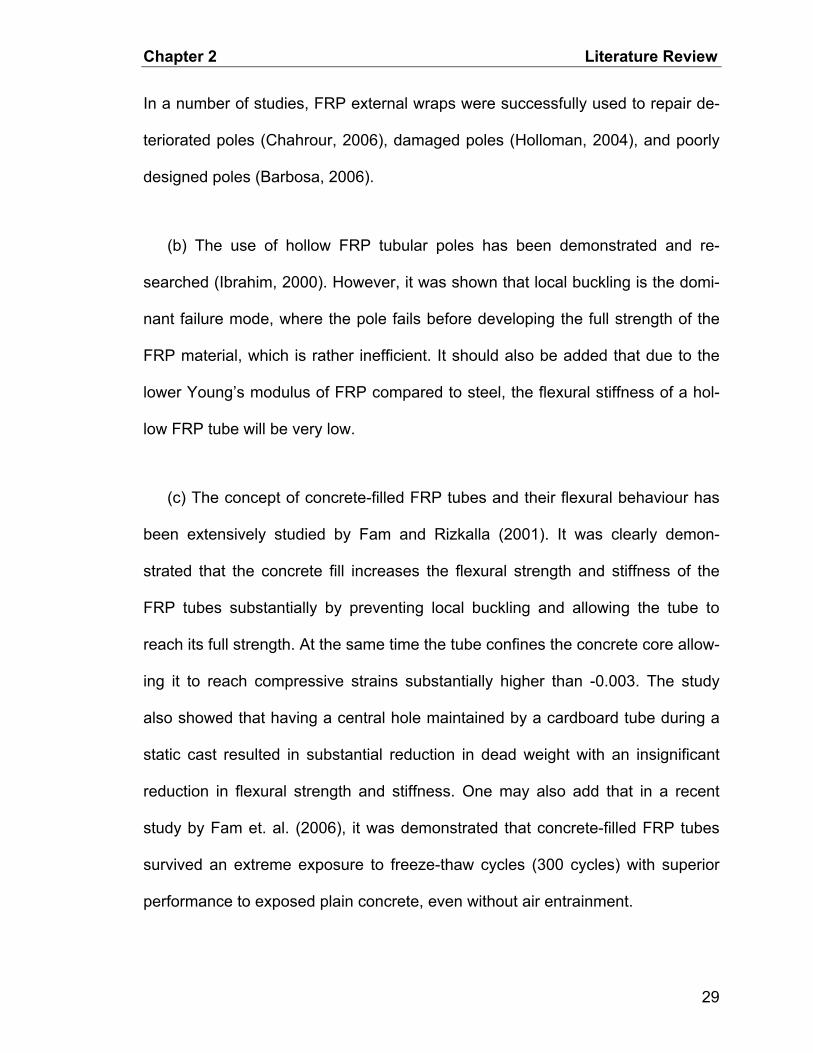
Chapter 2 Literature Review
In a number of studies, FRP external wraps were successfully used to repair de-
teriorated poles (Chahrour, 2006), damaged poles (Holloman, 2004), and poorly
designed poles (Barbosa, 2006).
(b) The use of hollow FRP tubular poles has been demonstrated and re-
searched (Ibrahim, 2000). However, it was shown that local buckling is the domi-
nant failure mode, where the pole fails before developing the full strength of the
FRP material, which is rather inefficient. It should also be added that due to the
lower Young’s modulus of FRP compared to steel, the flexural stiffness of a hol-
low FRP tube will be very low.
(c) The concept of concrete-filled FRP tubes and their flexural behaviour has
been extensively studied by Fam and Rizkalla (2001). It was clearly demon-
strated that the concrete fill increases the flexural strength and stiffness of the
FRP tubes substantially by preventing local buckling and allowing the tube to
reach its full strength. At the same time the tube confines the concrete core allow-
ing it to reach compressive strains substantially higher than -0.003. The study
also showed that having a central hole maintained by a cardboard tube during a
static cast resulted in substantial reduction in dead weight with an insignificant
reduction in flexural strength and stiffness. One may also add that in a recent
study by Fam et. al. (2006), it was demonstrated that concrete-filled FRP tubes
survived an extreme exposure to freeze-thaw cycles (300 cycles) with superior
performance to exposed plain concrete, even without air entrainment.
29

Chapter 2 Literature Review
Based on these observations, the concept of spin-casting concrete into FRP
tubes emerged as a novel idea that could possibly capture several features and
advantages of the systems described earlier, all combined in a new system. The
FRP tube provides the formwork, the reinforcement and the protection for the
spun-cast concrete. The spun cast concrete wall is thin, dense and is of high
quality. Even if longitudinal steel reinforcement or prestressing is added, it would
be well protected from corrosion and the concrete cover doesn’t need to be as
thick as in conventional poles. The system also has the advantage of being quite
elastic with insignificant residual deformations upon unloading, even near ulti-
mate. This is a very desirable feature in poles, particularly post exposure to se-
vere loading such as in hurricanes, as reported by Fouad (1994).
30

Chapter 2 Literature Review
Figure 2-1: Initial cost vs. height comparison between wooden and concrete poles (Fouad, 1992)
Figure 2-2: Several Concrete poles at various levels of deterioration (Courtesy of Fam).
31
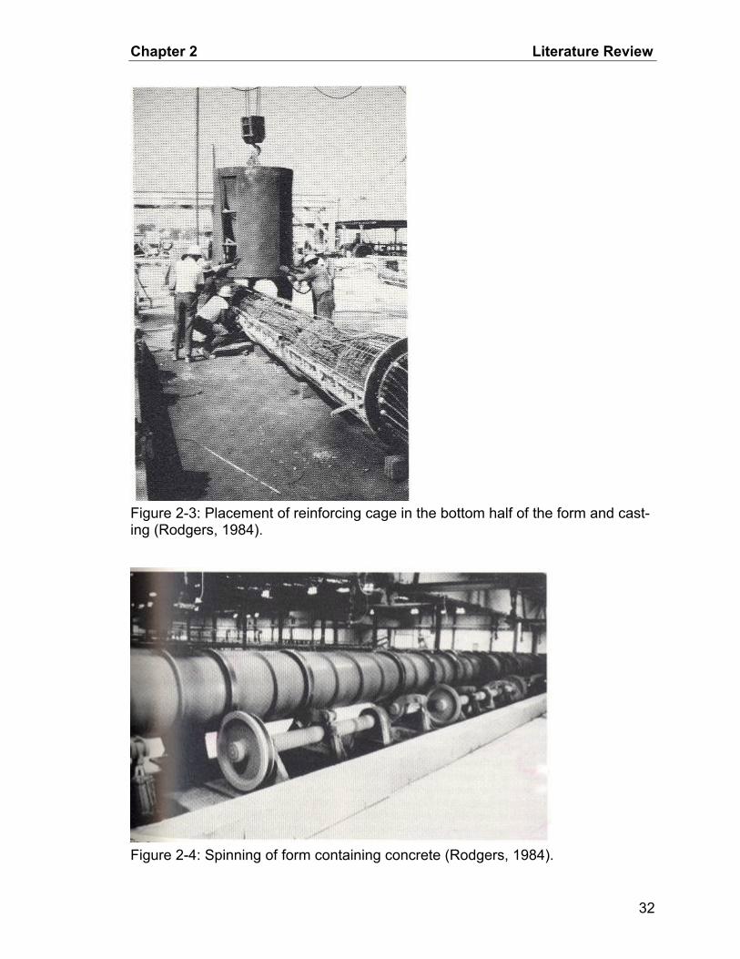
Chapter 2 Literature Review
Figure 2-3: Placement of reinforcing cage in the bottom half of the form and cast-ing (Rodgers, 1984).
Figure 2-4: Spinning of form containing concrete (Rodgers, 1984).
32

Chapter 2 Literature Review
Figure 2-5: Pole cracks and ground displacement showing the severity of hurri-cane Andrew (Fouad, 1994).
Figure 2-6: Pole deflecting during testing (Fouad, 1994).
33
Chapter 2 Literature Review
Figure 2-7: Theoretical and experimental load-deflection curves of 27 m long poles (Fouad, 1994).
Figure 2-8: Typical pole and a collapsed one (Barbosa, 2006).
34

Chapter 2 Literature Review
Inner Outer
Figure 2-9: Segregation of concrete during spinning (Barbosa et al., 2006).
Repaired Unreparied
Figure 2-10: Repaired and unrepaired specimens in testing frame (Barbosa et al., 2006).
Figure 2-11: Load-deflection plot of CFRP-repaired pole (Barbosa et al., 2006).
35

Chapter 2 Literature Review
Figure 2-12: Damage induced by car collision in Georgia (Holloman, 2004).
Figure 2-13: Local buckling of hollow GFRP tubular pole (Ibrahim, 2000).
36
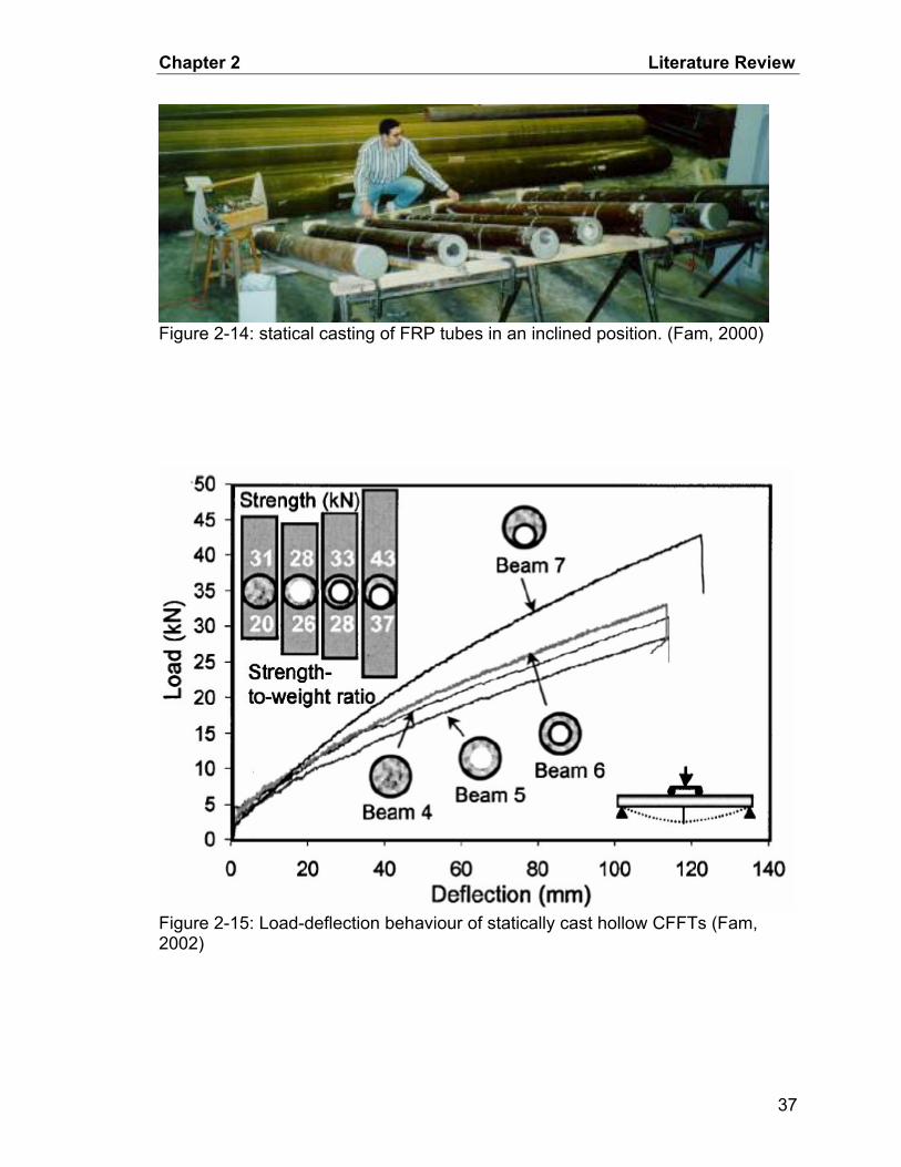
Chapter 2 Literature Review
Figure 2-14: statical casting of FRP tubes in an inclined position. (Fam, 2000)
Figure 2-15: Load-deflection behaviour of statically cast hollow CFFTs (Fam, 2002)
37

Chapter 2 Literature Review
Figure 2-16: Progressive failure of steel-reinforced CFFT B3. (Cole & Fam, 2006)
Figure 2-17: Production of prestressed CFFTs (Fam & Mandal, 2006).
38

Chapter 2 Literature Review
Figure 2-18: Fabrication of Prestressed CFFTs (Mandal & Fam, 2006).
Figure 2-19: Comparing prestressed CFFT to control specimen (Mandal & Fam, 2006).
39

Chapter 2 Literature Review
Figure 2-20: Prestressed and Regular CFFTs Moment-Curvature Comparison (Fam, 2006)
40

Chapter 3 Experimental Investigation
CHAPTER 3 : EXPERIMENTAL INVESTIGATION
General
The experimental program included an investigation of spun-cast concrete-
filled GFRP tubes (SCFTs) in flexure, by testing nine beam specimens, as well as
an investigation of the bond strength of SCFTs by testing six push-off specimens.
The parameters studied in the flexural investigation were the effect of the con-
crete wall thickness, the effect of the laminate structure of the tube, and the effect
of the addition of steel rebar. Eight of the beam specimens were fabricated by fill-
ing filament-wound circular GFRP tubes with concrete, seven of which were
spun-cast, and contained a central hole, while the eighth was statically cast and
completely filled. Of the spun cast specimens, one had eight No. 10 rebars ar-
ranged in an axisymmetric pattern with about 25 mm concrete clear cover, and
one had a concrete wall thickness of 45 mm, while the rest had a nominal wall
thickness of 65 mm. The ninth specimen was a conventional prestressed spun-
cast pole with a comparable length and diameter for comparison with the SCFT
specimens. In this chapter, the details of test specimens, parameters, fabrication
process, instrumentation, test setup, and testing procedures are presented, along
with a description of the properties of the materials used.
Materials Used in Test Specimens
The materials used to fabricate the test specimens were GFRP tubes, con-
crete, and various steel reinforcement. The mechanical properties of concrete
were obtained from the manufacturer, while those of the GFRP tubes were estab-
41

Chapter 3 Experimental Investigation
lished from tensile coupon tests and the classical lamination theory. The me-
chanical properties of the steel rebar were adopted from the Cole (2005) study,
which used similar steel.
GFRP Tubes
The tubes were fabricated by Ameron International’s Fibreglass Composite
Pipe Division in Burkburnett, Texas, using the filament-winding method and had
about 51% fibre volume fraction. Standard E-glass roving was wound around a
cylindrical mandrel. A thin liner was used to prevent adhesion. A layer of sand
was also included in two of the tubes to increase the wall thickness in order to
increase the buckling resistance of the tubes. Five different tubes, designated as
T1 to T5, were used. The tubes physical, mechanical, and geometrical properties
are shown in Table 3.1. Each tube had some layers oriented in the longitudinal
direction at angles of 8, 9 or 10 degrees and other layers in the hoop direction at
angles of 86 or 88 degrees relative to the longitudinal direction, as given in Table
3.2. The ratio of the thickness of the total layers in the axial to hoop direction is
given in Table 3.1. The mechanical properties given in Table 3.1 are all predicted
using the Classical Lamination Theory (CLT).
Concrete
The same concrete mixture was used to fabricate all test specimens at Utility
Structures Inc.. During the pour of every specimen standard size (4” by 8”) cylin-
ders were cast to determine the concrete strength.
42
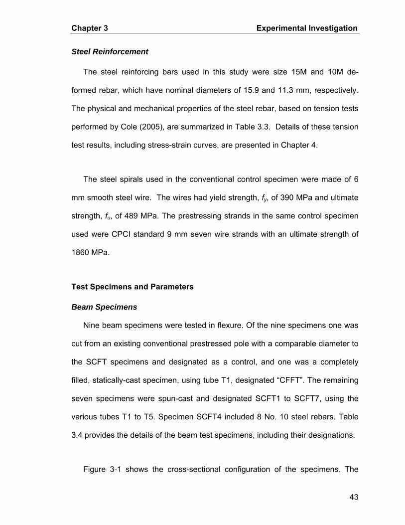
Chapter 3 Experimental Investigation
Steel Reinforcement
The steel reinforcing bars used in this study were size 15M and 10M de-
formed rebar, which have nominal diameters of 15.9 and 11.3 mm, respectively.
The physical and mechanical properties of the steel rebar, based on tension tests
performed by Cole (2005), are summarized in Table 3.3. Details of these tension
test results, including stress-strain curves, are presented in Chapter 4.
The steel spirals used in the conventional control specimen were made of 6
mm smooth steel wire. The wires had yield strength, fy, of 390 MPa and ultimate
strength, fu, of 489 MPa. The prestressing strands in the same control specimen
used were CPCI standard 9 mm seven wire strands with an ultimate strength of
1860 MPa.
Test Specimens and Parameters
Beam Specimens
Nine beam specimens were tested in flexure. Of the nine specimens one was
cut from an existing conventional prestressed pole with a comparable diameter to
the SCFT specimens and designated as a control, and one was a completely
filled, statically-cast specimen, using tube T1, designated “CFFT”. The remaining
seven specimens were spun-cast and designated SCFT1 to SCFT7, using the
various tubes T1 to T5. Specimen SCFT4 included 8 No. 10 steel rebars. Table
3.4 provides the details of the beam test specimens, including their designations.
Figure 3-1 shows the cross-sectional configuration of the specimens. The
43

Chapter 3 Experimental Investigation
beam specimens were 2.85 m long, except for specimen SCFT4 which was 2.75
m long, and the control specimen, which was 2.58 m long. The span of all speci-
mens was 2.65 m, except for specimens SCFT3 and SCFT4, which had a span
of 2.55 m, and the “control” specimen, which had a span of 2.46 m. These
lengths gave a span to diameter ratio of approximately 8.5. Cole (2005) showed
that for CFFTs with similar tubes, specimens tested with a span to diameter ratio
as low as two failed in flexure. As such, it’s believed that the beams tested in this
study are governed by flexure.
The beam specimens were designed to study the effects of several parame-
ters, and were compared to each other as follows:
1) Specimens CFFT, SCFT1 and SCFT2 were designed to determine the effect
of the concrete wall thickness on the behaviour of SCFTs. All three specimens
were fabricated from the same tube, T1, but CFFT was completely filled and
statically cast, whereas SCFT1 and SCFT2 had nominal concrete wall thick-
nesses of 45 mm and 65 mm, respectively, and were spun-cast.
2) Specimens SCFT3 and SCFT4 were compared to examine the effect of the
addition of steel reinforcement on the flexural performance of spun-cast con-
crete-filled GFRP tubes. The two specimens were made from tube T2, and
had a similar concrete wall thickness, but specimen SCFT4 had eight No. 10
steel reinforcing bars distributed axsisymetrically around the perimeter with a
25 mm concrete cover. It is likely that the tube will protect the steel reinforce-
44
Chapter 3 Experimental Investigation
ment from corrosion, and hence using FRP rebar instead of steel rebar is un-
necessary.
3) The effect of the GFRP tube, more specifically the laminate structure and
thickness, was studied through specimens SCFT2, SCFT3, SCFT5, SCFT6
and SCFT7, which had relatively similar concrete wall thicknesses, but were
fabricated from different tubes.
4) Specimens SCFT2, SCFT3 and SCFT6 were also compared to the control
specimen to determine how SCFT’s behaved when compared with the exist-
ing conventional poles. The specimens were selected because they had a
similar reinforcement index (ω), which is the reinforcement ratio normalized
with respect to material strength, to the control specimen as discussed in de-
tail in Chapter 4.
5) The effect of unloading and reloading, at a service load level, was studied in
all specimens by unloading at a load level approximately one half of the ex-
pected ultimate load and reloading to failure.
The results of the experimental investigation of the flexural behaviour of
SCFTs were also used to verify the analytical model, developed to predict the
moment-curvature response of SCFTs. The flexure behaviour model of SCFTs is
discussed in detail in Chapter 5. The push-off specimens were of two lengths to
determine the effect of length on bond behaviour.
45

Chapter 3 Experimental Investigation
Push-Off Specimens
An additional SCFT specimen was fabricated using tube T2 and was cut into
six short stub specimens, as shown in Table 3.5. Three specimens (S1 to S3)
were 300 mm long and the other three (L1 to L3) were 600 mm log. These stubs
were essentially push-off specimens tested to determine the bond behaviour and
strength at the interface between the tube and the concrete core.
Fabrication of Test Specimens
Beam Specimens
The hollow GFRP tubes were cut to the proper length, using a jigsaw and a
special blade, as shown in Figure 3-2, and were delivered to the pre-cast plant,
which is specialized in concrete pole fabrication. The tubes were placed in the
lower half of the conventional steel form as shown in Figure 3-3. The GFRP tube
was prevented from rotating inside the form by placing rubber pads between
them. The tube was also prevented from sliding longitudinally inside the form by
bolting small steel angles to the form as shown in Figure 3-3. For specimen
SCFT4 the steel cage was inserted into the tube at this point. This steel cage
consisted of eight No. 10 bars welded, at equal intervals, to a steel ring on both
ends, as shown in Figure 3-4. Concrete was then placed manually into the GFRP
tube from one end, with the other end sealed. Metal end plugs were fabricated in
the plant to prevent the wet concrete from escaping from the ends. Once a prede-
termined amount of concrete was placed and spread inside the tube, the other
end plug was secured in place and the top half of the form was placed, as shown
in Figure 3-5. The two halves of the form were then bolted together and trans-
46
Chapter 3 Experimental Investigation
ported to the spinning machine, where the entire arrangement was spun for there
to four minutes, first at 400 rpm then at 600 rpm, as shown in Figure 3-5. After
which the specimens were steam cured for sixteen hours and then placed in
open air. For fabricating the CFFT specimen, the GFRP tube was placed verti-
cally on a sealed end and filled with concrete from the top, as shown in Figure
3-6.
Push-Off Specimens
The push-off stub specimens were cut from an additional, long, SCFT speci-
men that was fabricated for that purpose, using a diamond-tip saw as shown in
Figure 3-7. Special care was taken to ensure a square and smooth cut at each
end.
Test Setup and Loading Scheme of Beam Specimens
Specimen CFFT, SCFT1, and SCFT2 were tested in four-point bending with a
span of 2.65 m and a 0.5 m distance between the loading points. Specimens
SCFT3 to SCFT7 and the control specimen were tested in three-point bending
with a span of 2.55 m for SCFT3 and SCFT4, a span of 2.65 m for SCFT5 to
SCFT7 and a span of 2.46 for the control. Specimen SCFT4 was accidentally cut
100 mm shorter than was intended, therefore, its span was 2.55 m, and since
specimen SCFT3 was designated for comparison with SCFT4, it was also tested
using a 2.55 m span. The control conventional specimen, which was only avail-
able at a 2.58 m length, was tested using a span of 2.46 m. Specimen SCFT2
failed prematurely near the support due to a defect in the tube. As such, the test
47
Chapter 3 Experimental Investigation
was repeated in three-point bending using a shorter span of 2.07 m. After testing
SCFT2 it was decided to maximize the length of the shear span to ensure flexural
failure and for this reason it was decided to switch to the three-point bending con-
figuration. The details of the test setups are shown in Figure 3-8 and Figure 3-9.
At the support and loading points, 90 mm wide steel channel sections were used
to accommodate the specimens. Quick-set plaster was moulded into the chan-
nels to conform to the curved surface.
The load was applied under stroke control, using a 900 kN Reihle loading ma-
chine, at a rate of 1 mm/min. All specimens were unloaded and then reloaded to
failure at a load of approximately 165 kN, to examine the stiffness at service load
level. Specimen SCFT4 was subjected to an additional unloading and reloading
at a 335 kN load.
Test Setup and Loading Scheme of Push-Off Specimens
The push-off test setup is shown in Figure 3-12. A special steel base was fab-
ricated to support the tube during the push off tests. This consisted of a steel
plate with eight 50 mm thick steel blocks welded to it forming a circular pattern.
On the blocks, 5 mm thick steel strips were welded to guide the tube in place
such that only half of the tube thickness is supported by the blocks. This ar-
rangement was to ensure that when the concrete core is pushed from the top, it
does not rub against the steel blocks. The top surface of the specimen was cov-
ered with a thin rubber sheet and another circular steel plate was used to apply
48

Chapter 3 Experimental Investigation
load to the concrete core only, and not the tube. The load was applied at a rate of
1mm/min.
Instrumentation
Details of the instrumentation for the four-point bending test specimens are
shown in Figure 3-10, while those for the three-point bending test specimens are
shown in Figure 3-11. The following sections provide details for the instrumenta-
tion in each case.
Bending Tests
Electrical resistance strain gauges of type FLA-6-11-5L, with 5 mm gauge
length, 120 ohms resistance and +/- 0.00001 strain error, were used. These
gauges were manufactured by Sokki Kenkyujo Co. Ltd., Japan and were at-
tached using the M-Bond 200 adhesive system. A total of six strain gauges were
attached to the outer surface of each tube, four of which were attached longitudi-
nally, two at the extreme compression fibres and two at the extreme tension fi-
bres, and two circumferential gauges on the compression side. One of the two
longitudinal strain gauges was placed at midspan and the other was placed 75
mm away. The GFRP tubes’ surfaces were sanded to remove the protective UV
coating before installation of strain gauges. No strain gauges were attached to
the control specimen. Displacement-type strain transducers (PI-gauges) of 200
mm gauge length, with an error of +/- 0.00001 strain were also used on all beam
specimens to measure the average longitudinal strains at the top and bottom sur-
faces at mid-span. The mid-span deflections were monitored using two 100 mm
49

Chapter 3 Experimental Investigation
linear potentiometers (LPs). Additional 25 mm LPs were used to monitor slip be-
tween the GFRP tube and the concrete core, as well as any deflection at both of
the supports. Details of the instrumentation for bending tests are shown in Figure
3-10. All the LPs had an error of +/- 0.1 mm
The load and stroke from the Reihle loading machine, as well as the readings
from the LPs, PI-gauges, and strain gauges were recorded during the test using a
Vishay Micro Measurements System 5000 and the data acquisition program
Strain Smart.
Bond Slip Tests
Displacement of the concrete core relative to the tube was monitored using
two 100 mm LPs on the upper end of the specimen as well as the stroke from the
loading machine. The load was measured using the load cell built into the Reihle
machine. The load and stroke and the readings from the LPs were recorded dur-
ing the test using a Vishay Micro Measurements System 5000 and the data ac-
quisition program Strain Smart.
GFRP Tube Coupon Tests
The mechanical properties of the GFRP tubes were determined by testing
three coupons cut from each tube in the longitudinal direction under uniaxial ten-
sion. Coupons were 175 x 25 mm, with end tabs that were 75 mm long on either
end, leaving a clear length of 25 mm. The end tabs were used to eliminate the
effect of curvature of the tubes and ensure a flat surface to facilitate a uniform
50
Chapter 3 Experimental Investigation
grip in the testing machine. The tabs were made of two layers of epoxy impreg-
nated unidirectional GFRP sheets bonded to each side of the coupons. It is im-
portant to note that ASTM Standard D 3039/D 3039M-95a recommends using
longer 300 x 25 mm coupons for tension, but, in a recent study (Mandal, 2004), it
was found that for filament-wound GFRP tubes, long coupons for tension tests
failed at strains substantially lower than those measured in test beams at ulti-
mate, whereas short coupons attained failure strains similar to those measured in
beams at ultimate. This was attributed to the helical geometry of the fibres, which
results in lack of continuity of some of the fibres between grips, particularly when
long and narrow coupons are used, as shown schematically in Figure 3-13(a).
The Figure shows that the bandwidth of continuous fibres is smaller in the long
coupons than in the short ones. Since the discontinuous fibres do not contribute
fully to the tensile strength of the coupon, this results in underestimating the ten-
sile strength of the tube. The coupons were instrumented on both sides with a 5
mm electrical resistance strain gauge mounted longitudinally, as shown in Figure
3-13(b). Tension tests were performed using an Instron Model 1350 testing ma-
chine. It should be noted, however, that hydraulic grips were used by Mandal
(2004), whereas mechanical grips were used in this study, as shown in Figure
3-13(c). As such, even though short coupons were used in this study, they did not
reach the full strength of the tubes encountered in the beam tests. Loads from the
Instron loading machine and strain readings were recorded using a Vishay Micro
Measurements System 5000 along with the data acquisition program Strain
Smart. Details of tensile coupon test results are discussed in Chapter 4.
51
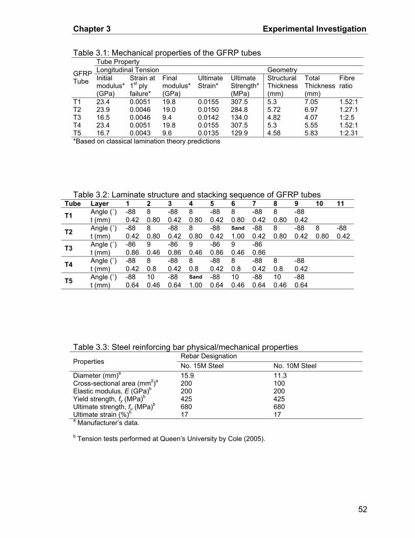
Chapter 3 Experimental Investigation
Table 3.1: Mechanical properties of the GFRP tubes Tube Property Longitudinal Tension Geometry GFRP
Tube Initial modulus* (GPa)
Strain at 1st ply failure*
Final modulus* (GPa)
Ultimate Strain*
Ultimate Strength* (MPa)
Structural Thickness (mm)
Total Thickness (mm)
Fibre ratio
T1 23.4 0.0051 19.8 0.0155 307.5 5.3 7.05 1.52:1 T2 23.9 0.0046 19.0 0.0150 284.8 5.72 6.97 1.27:1 T3 16.5 0.0046 9.4 0.0142 134.0 4.82 4.07 1:2.5 T4 23.4 0.0051 19.8 0.0155 307.5 5.3 5.55 1.52:1 T5 16.7 0.0043 9.6 0.0135 129.9 4.58 5.83 1:2.31 *Based on classical lamination theory predictions
Table 3.2: Laminate structure and stacking sequence of GFRP tubes Tube Layer 1 2 3 4 5 6 7 8 9 10 11
Angle (˚) -88 8 -88 8 -88 8 -88 8 -88 T1 t (mm) 0.42 0.80 0.42 0.80 0.42 0.80 0.42 0.80 0.42 Angle (˚) -88 8 -88 8 -88 Sand -88 8 -88 8 -88 T2 t (mm) 0.42 0.80 0.42 0.80 0.42 1.00 0.42 0.80 0.42 0.80 0.42 Angle (˚) -86 9 -86 9 -86 9 -86 T3 t (mm) 0.86 0.46 0.86 0.46 0.86 0.46 0.86 Angle (˚) -88 8 -88 8 -88 8 -88 8 -88 T4 t (mm) 0.42 0.8 0.42 0.8 0.42 0.8 0.42 0.8 0.42 Angle (˚) -88 10 -88 Sand -88 10 -88 10 -88 T5 t (mm) 0.64 0.46 0.64 1.00 0.64 0.46 0.64 0.46 0.64
Table 3.3: Steel reinforcing bar physical/mechanical properties Rebar Designation
Properties No. 15M Steel No. 10M Steel Diameter (mm)a 15.9 11.3 Cross-sectional area (mm2)a 200 100 Elastic modulus, E (GPa)b 200 200 Yield strength, fy (MPa)b 425 425 Ultimate strength, fu (MPa)b 680 680 Ultimate strain (%)b 17 17 a Manufacturer’s data.
b Tension tests performed at Queen’s University by Cole (2005).
52
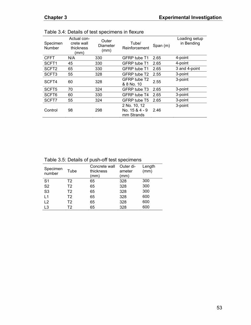
Chapter 3 Experimental Investigation
Table 3.4: Details of test specimens in flexure
Specimen Number
Actual con-crete wall thickness
(mm)
Outer Diameter
(mm)
Tube/ Reinforcement Span (m)
Loading setup in Bending
CFFT N/A 330 GFRP tube T1 2.65 4-point SCFT1 45 330 GFRP tube T1 2.65 4-point SCFT2 65 330 GFRP tube T1 2.65 3 and 4-point SCFT3 55 328 GFRP tube T2 2.55 3-point
SCFT4 60 328 GFRP tube T2 & 8 No. 10 2.55 3-point
SCFT5 70 324 GFRP tube T3 2.65 3-point SCFT6 60 330 GFRP tube T4 2.65 3-point SCFT7 55 324 GFRP tube T5 2.65 3-point
Control 98 298 2 No. 10, 12 No. 15 & 4 - 9 mm Strands
2.46 3-point
Table 3.5: Details of push-off test specimens
Specimen number Tube
Concrete wall thickness (mm)
Outer di-ameter (mm)
Length (mm)
S1 T2 65 328 300 S2 T2 65 328 300 S3 T2 65 328 300 L1 T2 65 328 600 L2 T2 65 328 600 L3 T2 65 328 600
53
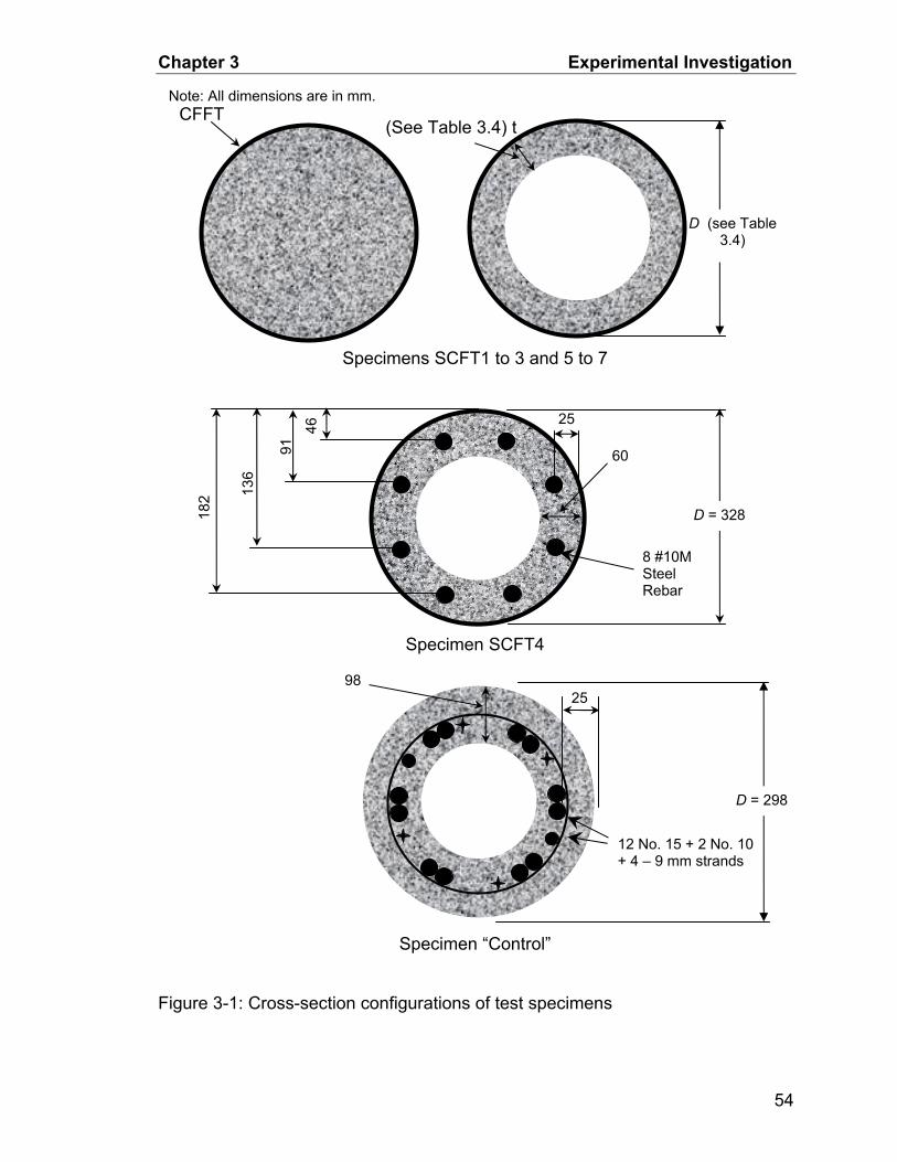
Chapter 3 Experimental Investigation
Specimen “Control”
Figure 3-1: Cross-section configurations of test specimens
D = 298
25
12 No. 15 + 2 No. 10 + 4 – 9 mm strands
Specimen SCFT4
D = 328
46
91
182
25
8 #10M Steel Rebar
136
60
98
D (see Table 3.4)
Specimens SCFT1 to 3 and 5 to 7
(See Table 3.4) tCFFT
Note: All dimensions are in mm.
54
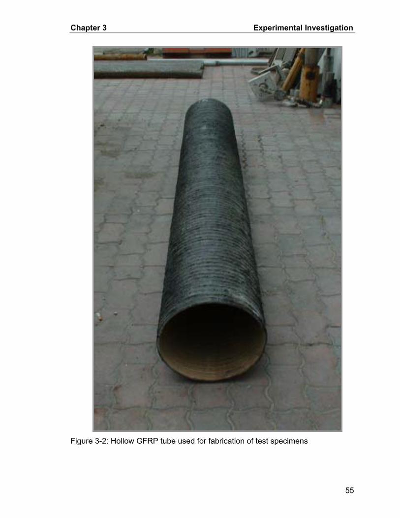
Chapter 3 Experimental Investigation
Figure 3-2: Hollow GFRP tube used for fabrication of test specimens
55
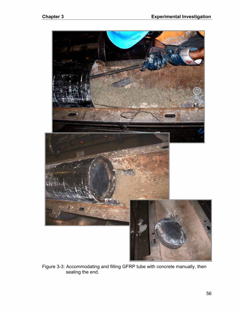
Chapter 3 Experimental Investigation
Figure 3-3: Accommodating and filling GFRP tube with concrete manually, then sealing the end.
56
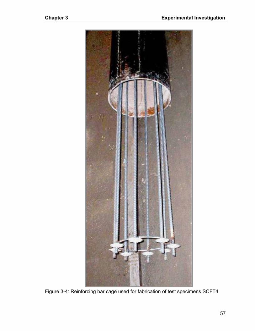
Chapter 3 Experimental Investigation
Figure 3-4: Reinforcing bar cage used for fabrication of test specimens SCFT4
57
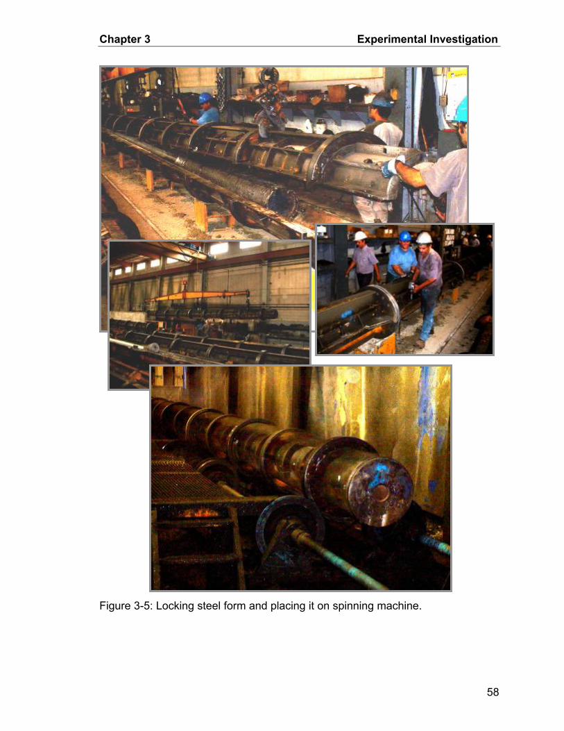
Chapter 3 Experimental Investigation
Figure 3-5: Locking steel form and placing it on spinning machine.
58

Chapter 3 Experimental Investigation
Figure 3-6: Fabrication of CFFT specimen.
59
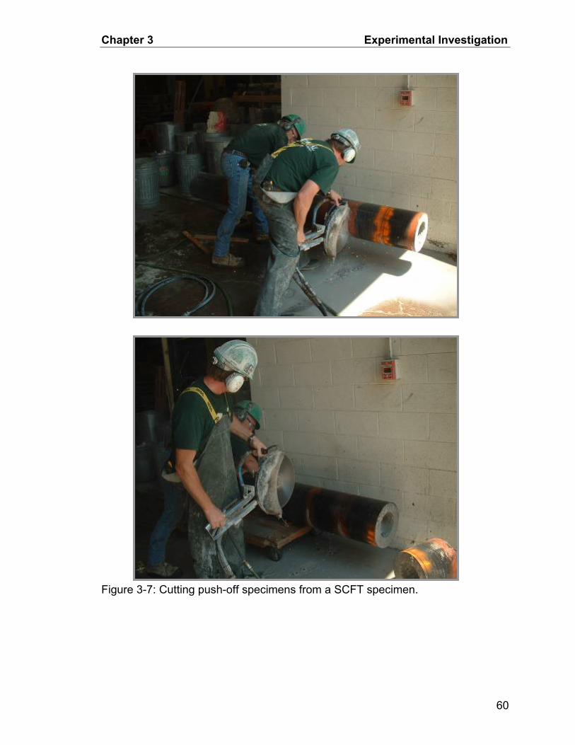
Chapter 3 Experimental Investigation
Figure 3-7: Cutting push-off specimens from a SCFT specimen.
60

Chapter 3 Experimental Investigation
(a) Schematic of test setup for CFFT, SCFT1 and SCFT2
Steel spreader beam Test beam
2.65 m
500 mm Roller support
Roller
(b) Schematic of test setup for SCFT3 to SCFT7 and the control
Test beam
Roller support
2.46 m or 2.55 m or 2.65 m
Figure 3-8: Test setup for flexural specimens.
61

Chapter 3 Experimental Investigation
Figure 3-9: Overall 3-point and 4-point bending test setups.
62
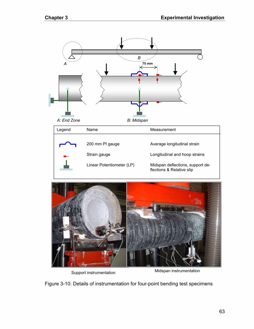
Chapter 3 Experimental Investigation
Legend Name Measurement
200 mm PI gauge Average longitudinal strain Strain gauge Longitudinal and hoop strains
Linear Potentiometer (LP) Midspan deflections, support de-flections & Relative slip
A B
A: End Zone B: Midspan
Support instrumentation Midspan instrumentation
75 mm
Figure 3-10: Details of instrumentation for four-point bending test specimens
63

Chapter 3 Experimental Investigation
Midspan instrumentation
~50 mm
A B
75 mm
A: End Zone B: Midspan
Legend Name Measurement
200 mm PI gauge Average longitudinal strain Strain gauge Longitudinal and hoop strains
Linear potentiometer (LP) Midspan deflections, support de-flections & Relative slip
Figure 3-11: Details of instrumentation for three-point bending test specimens
64

Chapter 3 Experimental Investigation
300 mm or 600 mm
Steel Blocks
LP
Steel Plate
Steel Plate
Figure 3-12: Push-off test setup
(a) Short vs. long coupons (b) Details of instrumentation (c) Testing of
θθb1
b2
Bandwidth b1 > b2
Short Long Coupon Coupon
75 mm
25 mm
75 mm A A
Coupon GFRP Tabs
Front View Side View
25 mm
Section A-A
coupons Figure 3-13: Details of coupons used to determine mechanical properties of tubes
65
Chapter 4 Test Results and Discussion
CHAPTER 4 : TEST RESULTS AND DISCUSSION
General
This chapter presents the results of the ancillary material tests, the nine beam
specimens tested in flexure, and the six push-off spun-cast test specimens tested
for bond strength. The tensile mechanical properties of the GFRP tubes, in the
longitudinal direction, are established by testing coupons cut from the tubes. The
steel rebar mechanical properties are established using standard tension tests.
The compressive strength of the concrete used in the spun-cast specimens is de-
termined using standard concrete tests performed by the manufacturer on stati-
cally-cast cylinders. The flexural behaviour of the beam specimens is evaluated
based on “load-deflection”, “load-strain” and “moment-curvature” responses,
while the push-off specimens are used to establish the “bond stress-slip” re-
sponse. The effects of the size of the central hole, the presence of steel rebar,
and the different GFRP tube’s laminate structures on the flexural strength and
overall behaviour of spun-cast FRP tubes (SCFTs) are discussed in detail. A
comparison with a conventional prestressed spun-cast pole, also tested in this
study, is made.
Ancillary Test Results
Tension Tests of GFRP Tube Coupons
The longitudinal stress-strain curves, obtained through tensile coupon tests,
for the five GFRP tubes used in this study are shown in Figure 4-1. The coupons
were 175 x 25 mm with 75 x 25 mm end tabs and a clear distance of 25 mm be-
tween the tabs. The stress-strain curves showed a somewhat nonlinear behav-
66

Chapter 4 Test Results and Discussion
iour, and the failure strains of the coupons were lower than those measured in
tension at failure of the SCFT beam tests. The lower failure strains of coupons
are generally attributed to the helical nature of the fibres within the cylindrical
tubes, and as such, some fibres are discontinuous between the end tabs within
the width of the coupons. For this reason the distance between the tabs is kept at
a minimum. This, however, did not prevent the premature failure because me-
chanical grips were used. The nonlinear behaviour of the GFRP tube is caused
by the progressive failure of the GFRP laminate. The first stage is the splitting of
the transverse (circumferential) layers, followed by failure of the longitudinal lay-
ers as loading continues. Nonlinearity in GFRP laminates may also be caused by
the nonlinear behaviour of the epoxy resin. The results of the tension coupon
tests are summarized in Table 4-1. Figure 4-1 also shows the actual failure
strains of the tubes as measured in the full scale SCFT beam specimens that
failed in tension. Figure 4-3 shows a typical failure of the GFRP coupons in ten-
sion.
It should be noted that when hydraulic grips were used by Mandal (2004) to
test similar coupons, failure strains very similar to those measured in the full
scale beams were achieved. Mandal (2004) also concluded that the longitudinal
tensile and compressive behaviour of the GFRP tubes is quite similar. This was
attributed to the presence of sufficient hoop fibres to provide enough support for
the longitudinal fibres and prevent buckling on the microscopic scale.
67

Chapter 4 Test Results and Discussion
Tensile Behavior of Steel Reinforcement
Cole & Fam (2005) performed three tensile tests on 10M and two tests on
15M steel rebar of the same grade as the rebar used in specimens SCFT4 and
the control pole. The stress-strain curves of the steel rebar are shown in Figure
4-2. They show a linear elastic region, followed by a short yield plateau at a
strength of about 425 MPa until a strain of about 0.011, followed by a strain hard-
ening region, with an ultimate strength of about 680 MPa. Fracture occurred at a
strain of about 0.17, after necking.
The steel strands used in the control prestressed specimen were 9 mm di-
ameter seven-wire strands with nominal tensile strength of 1860 MPa (CPCI,
1996). The steel spiral reinforcement of the same specimen was 6 mm diameter
smooth wire of 390 MPa nominal yield strength.
Concrete Compression Tests
Standard compression tests on statically-cast concrete cylinders were per-
formed 28 days after casting of most specimens in the precast plant where the
specimens were fabricated. The results of these tests are presented in Table 4-2.
In general, the compressive strength ranged from 55 to 71 MPa. It should be
noted that this is a relatively higher strength than most precast concrete due to
the low water-cement ratio required to achieve low slump in conventional spun-
cast concrete.
68

Chapter 4 Test Results and Discussion
Test Results of Pole Beam Specimens
In this section, the flexural behaviour of each specimen is presented sepa-
rately first. The figures presented are the “load-deflection”, “load-longitudinal
strain”, “moment-curvature”, “load-hoop strain”, and “load-slip responses”, as well
as pictures of the failure mode. The plots for specimen CFFT are shown in Figure
4-4 to Figure 4-9. Those of specimen SCFT1 are in Figure 4-10 to Figure 4-15.
Figure 4-16 to Figure 4-21 are for specimen SCFT2. Figure 4-22 to Figure 4-27
are for specimen SCFT3. Figure 4-28 to Figure 4-33 are for specimen SCFT4.
Figure 4-34 to Figure 4-39 are for specimen SCFT5. Figure 4-40 to Figure 4-45
are for specimen SCFT6. Figure 4-46 to Figure 4-51 are for specimen SCFT7.
Figure 4-52 to Figure 4-54 are for the control. Subsequently, flexural responses
of the specimens are compared on the same plot to evaluate the effects of vari-
ous parameters. In the comparison figures, cyclic loading paths were removed
from the graphs for clarity.
For specimen SCFT2, premature local failure occurred at one support when it
was first tested in four-point bending with a span of 2.65 m. After investigation, it
was found that a pre-existing defect (a tearing crack extending about 80 mm from
one end of the tube in the longitudinal direction) caused the premature failure as
the crack propagated over the support. It is believed that this crack was caused
by damage during shipping and handling. As such, specimen SCFT2 was tested
again in three-point bending with a smaller span of 2.07 m, where it failed in flex-
ure, as expected, at mid span similar to the other specimens. Therefore, the load-
69

Chapter 4 Test Results and Discussion
deflection and moment-curvature graphs for this specimen include two plots, one
for the first test, and the other for the second test.
General Flexural Behavior of SCFT Pole Specimens
The load-deflection responses of the SCFT pole beam specimens indicate
that the specimens experienced a small progressive reduction in stiffness. First
cracking in the concrete occurs at a relatively low load level, compared to ulti-
mate load and was detected by a sudden drop in load and a subsequent reduc-
tion in stiffness. As more cracking occurred, the behaviour became slightly
nonlinear until failure. Specimen SCFT4 (Figure 4-28), with steel rebar, exhibited
an additional reduction in stiffness as a result of yielding of the bottom layer of
rebar. All the specimens continued to resist load until the GFRP tube or the con-
crete core failed, as will be discussed later. Important parameters describing the
flexural response of each specimen are: the cracking moment, Mcr, yielding mo-
ment, My (for specimen SCFT4 and control only), maximum moment, Mmax, cur-
vature at maximum moment, ψmax, and the top and bottom axial strains at maxi-
mum load, εt and εb, respectively. These parameters are summarized in Table
4-3.
All the specimens were unloaded at approximately 165 kN, and reloaded to
failure, except for specimen SCFT7 which failed before reaching this load. This
load was approximately half the expected ultimate load of the reference speci-
men, CFFT, which was totally filled with concrete. As such, it was considered to
somewhat represent an upper limit to the expected service load level, based on
70

Chapter 4 Test Results and Discussion
an assumed safety factor of two for specimen CFFT. As already mentioned, the
load-deflection responses underwent some reduction in stiffness after cracking.
As a result, some permanent deflection, ranging from 3 mm to 13 mm, was ob-
served upon unloading. This permanent deflection is probably due to the cracks
in the concrete not closing completely after unloading as well as micro cracking of
the FRP tube laminate. Specimen SCFT4 (Figure 4-28) was additionally
unloaded at 335 kN, which is approximately 50 % of the estimated ultimate load
of this specimen, as it contained steel rebar. As expected, a larger permanent de-
flection was observed, as a result of the yielding of the rebar. It is also noted that
stiffness is slightly reduced, relative to that at the 165 kN load, due to excessive
yielding. Additional observations regarding permanent deflections will be given
when addressing the effects of various parameters.
Definition of Terminology used in Comparisons
In this section the terms FRP reinforcement ratio ρf, steel reinforcement ratio
ρs, prestressing reinforcement ratio ρps and reinforcement index ω, which are
used in subsequent sections to describe the effects of various parameters on the
flexural response of the specimens, are briefly discussed. The FRP reinforcement
ratio ρf is defined as the ratio of the cross-sectional area of the GFRP tube to the
cross sectional area of the concrete core as follows:
( )( ) (( ))
−=
− − − −0 FRP FRP
f 2o FRP o FRP conc
4 D t tρ
D 2t D 2t 2t 2 (4-1)
71

Chapter 4 Test Results and Discussion
where Do is the outer diameter of the tube, tFRP is the wall thickness of the tube
and tconc is the concrete wall thickness. The steel reinforcement ratio ρs, is de-
fined as the ratio of the area of all the steel rebar As,total, to the area of the con-
crete core, and is given by:
( ) (( ))s,total
s 2o FRP o FRP conc
4Aρ =
π D - 2t - D - 2t - 2t 2
)
(4-2)
Similarly, the prestressing reinforcement ratio ρps is defined as:
( ) (( )PS
PS 2o FRP o FRP conc
4Aρ =π D - 2t - D - 2t - 2t 2
(4-3)
where APS is the total area of prestressing strands. In order to facilitate the com-
parison between specimens with different types of reinforcement and concrete
strengths, the term reinforcement index ω is introduced, which is essentially the
sum of FRP and steel reinforcement ratios normalized with respect to the mate-
rial strengths (i.e. tensile strength of the GFRP tube, ffu, the tensile ultimate
strength of steel rebar, fsu, the tensile strength of steel strands, fpu, and the con-
crete compressive strength f ′c) as follows:
pufu suf s PS
c c
ff fω = ρ +ρ +ρf f
⎛ ⎞ ⎛ ⎞ ⎛ ⎞⎜ ⎟ ⎜ ⎟ ⎜ ⎟′ ′⎝ ⎠ ⎝ ⎠ ⎝ ⎠cf ′
(4-4)
The reinforcement indices for all beams are given in Table 4-3
Comparison between SCFT Poles and Conventional Spun Cast Pole
Figure 4-55 provides a comparison between the conventional spun-cast pole
“control” specimen and specimens SCFT2, 3 and 6. The reinforcement index ω of
the “control” was 57.5%, based on equation 4-4, excluding the first term of the
72
Chapter 4 Test Results and Discussion
FRP tube contribution. The reinforcement indices, ω, of SCFT2, 3 and 6 were all
50%, also calculated using equation 4-4, excluding the second and third terms of
the steel reinforcement contributions.
Figure 4-55 shows that moment-deflection curves in the beams, normalized to
account for the differences in span, diameter, and concrete strength. The figure
generally shows that the flexural strength of the new SCFT poles is comparable
to that of conventional partially prestressed spun-cast poles of a similar rein-
forcement index. Specimens SCFT2, 3 and 6 varied slightly in strength, despite
their similar reinforcement indices, because failure modes were not the same.
SCFT2 failed in tension, whereas SCFT3 and SCFT6 failed in compression. The
strength of the “control” specimen is limited by the concrete cover crushing and
spalling after yielding of some steel reinforcement.
It is also clear that SCFT poles are much lower in stiffness than the “control”
pole, due to the lower Young’s modulii of the tubes, which is about 19 and 20
GPa, relative to that of steel, which is 200 GPa. Additionally, the “control” speci-
men was prestressed.
Effect of Various Parameters
In the following sections, the effects of various parameters intended in this
study are evaluated by comparing the behaviour of different specimens. These
parameters are the concrete wall thickness, the steel rebar contribution and the
FRP tube laminate structure.
73

Chapter 4 Test Results and Discussion
Effect of Concrete Wall Thickness
Specimens SCFT1, SCFT2 and CFFT were all fabricated using the same
GFRP tube, T1, and the only variable was the concrete wall thickness. A com-
parison between the three specimens is presented in Figure 4-56 to Figure 4-62
in terms of the following responses: load-deflection, moment-curvature, moment-
longitudinal strain, moment-hoop strain in compression, moment-slip, moment-
neutral axis depth, and hoop strain-axial strain on the compression side. The ef-
fect of the concrete wall thickness is also summarized in Figure 4-63 to Figure
4-66, in terms the effect of inner-to-outer diameter ratio (Di / Do) on ultimate mo-
ment ratio of the hollow and totally filled tubes (Mu hollow / Mu full), on the ultimate
strength-to-self weight ratio (Pu / W), on the cracking moment ratio of hollow and
totally filled tubes (Mcr hollow / Mcr full), and on the neutral axis depth-to-outer diame-
ter ratio (C/Do).
It should be noted that Figure 4-56 is based on a four-point bending configura-
tion. Since specimen SCFT2 failed prematurely and was retested in three-point
bending, where it failed in flexure, the load-deflection curve of specimen SCFT2
is shown as a solid line until premature failure occurred. The ultimate flexural load
of this specimen is given as a horizontal line and is converted from the three-
point bending test to an equivalent load based on a four-point bending configura-
tion. The curve extension to the failure load is shown as a dotted line. In Figure
4-57 and Figure 4-61 the curvatures and neutral axis depth are calculated using
the top and bottom longitudinal strains measured on the surface of the FRP tube.
74
Chapter 4 Test Results and Discussion
As shown in Figure 4-56 and Figure 4-57, the initial flexural stiffness of
specimens SCFT1, SCFT2 and CFFT are somewhat similar. However, the differ-
ence lies in the cracking and ultimate loads. As the inner hole size is increased,
the cracking load is substantially reduced as shown in Figure 4-65. This is a di-
rect result of the reduction of the moment of inertia of the uncracked section.
This, however, doesn’t seem to affect the stiffness after cracking much, since the
moment of inertia of the cracked section is controlled to a much larger extent by
the FRP tube rather than the concrete core.
The cracking moments of specimens SCFT1 and SCFT2 were about 28 and
44 percent of that of specimen CFFT, respectively. The nonlinear variation of
cracking moment with respect to concrete thickness, reflected in Figure 4-65, is
due to the dependence of cracking moment on the moment of inertia of the cross
section, which is related to the fourth power of the outer and inner diameters.
Specimens SCFT2 and CFFT showed a comparable moment capacity,
whereas specimen SCFT1 showed a substantially lower ultimate moment, as
shown in Figure 4-57. This is attributed to the failure mode of specimen SCFT1,
which occurred by inward spalling of the very thin concrete wall, as shown in
Figure 4-15, before the FRP tube developed its full strength. Specimens SCFT2
and CFFT on the other hand failed in tension, as shown in Figure 4-21 and
Figure 4-9, respectively. This is also confirmed by the lower tensile strain of
SCFT1 at failure compared to specimens SCFT2 and CFFT, as shown in Figure
4-58.
75
Chapter 4 Test Results and Discussion
The slightly higher ultimate moment of specimen SCFT2 than CFFT (Figure
4-57) could be attributed to the three-point versus four-point bending testing con-
figuration. It is possible that the single loading point at mid-span has caused
some confinement of concrete on the compression side under the loading point,
which is the maximum moment section, resulting in a slightly higher moment ca-
pacity. It is also possible that the strength of spun-cast concrete is higher than
that of statically-cast concrete.
Figure 4-63 shows the variation of flexural strength, normalized with respect
to that of the totally filled tube, CFFT, with the inner-to-outer diameter ratio (Di /
Do), whereas Figure 4-64 shows the variation of flexural strength-to-weight ratio
(Pu / W) with (Di / Do).
Figure 4-64 shows that specimen SCFT2 had the highest flexural strength-to-
self weight ratio. From Figure 4-66 and Figure 4-63 it is concluded that for this
particular FRP tube, the optimum concrete wall thickness is between 45 mm and
65 mm. Since no other concrete wall thickness between these two values was
tested and since these two values are not too far apart, it is suggested that the 65
mm thick concrete wall of specimen SCFT2, which corresponds to a concrete
wall thickness-to-diameter ratio (tc /Do) of 0.2 is the recommended minimum
value, for this FRP tube, to be able to achieve the same flexural strength of a to-
tally filled tube at a minimum dead weight. In Chapter 5, a parametric study is
carried out using the developed analytical model to see if this ratio varies signifi-
76
Chapter 4 Test Results and Discussion
cantly for different tubes of various FRP tube thicknesses and laminate struc-
tures, or it is rather independent.
In Figure 4-60, it is interesting to note that specimen SCFT1, with the mini-
mum concrete thickness, showed distinctly smaller end slip values, whereas both
SCFT2 and CFFT showed similar values. This may be attributed to a slight ovali-
zation of the cross-section of SCFT1, a phenomena resulting from flexural curva-
ture, which is well known for thin tubes (Ibrahim et al., 2000). As this ovalization
is maximum at mid span and minimum at the ends, the different cross-sectional
geometries at midspan and the ends may have partially restrained the movement
of the concrete core relative to the FRP tube.
Figure 4-61 suggests that at low moments, the neutral axis depth varies,
where it is larger for a thinner concrete wall, but eventually not much variation is
seen at high moments. Figure 4-66 shows the variation of the average neutral
axis depth (over the whole range of loading) with the inner-to-outer diameter ra-
tio. The variation of the concrete wall thickness is also shown. It appears from
this figure that there is a specific (Di/Do) ratio at which the neutral axis depth is
equal to the concrete wall thickness; however, this may not necessarily be the
optimum (Di/Do) ratio from the flexural strength point of view. For example it was
shown earlier that the optimum Di/Do ratio was between 0.61 and 0.73, where as
the two curves in Figure 4-66 intercept at a Di/Do of 0.39.
77
Chapter 4 Test Results and Discussion
The variation of hoop tensile strains with longitudinal compressive strain at the
compression side of the tube is a good indication of the confinement effect of the
concrete core (Fam & Rizkalla, 2002). As shown in Figure 4-62 there is no dis-
tinct difference between the three curves, which suggests that the hole size has
no effect on this response. It should be mentioned, however, that confinement
effect in flexure is very small, even for totally-filled tubes (Fam & Rizkalla, 2002)
and if it was significant it would have been evident by distinctly bi-linear re-
sponses in Figure 4-62.
Effect of Presence of Rebar
Specimens SCFT3 and SCFT4 were fabricated using Tube 2 and tested using
the same configuration. The only difference was that specimen SCFT4 had 8 No.
10 steel rabars, whereas SCFT3 did not contain any steel reinforcement. As such
the reinforcement index ω, defined in equation 4-4, was 50.6 % and 62.5 % for
specimen SCFT3 and SCFT4, respectively. A comparison between the beams in
terms of “load-deflection”, “moment-curvature”, “load-longitudinal strain”, “load-
slip”, “moment-neutral axis depth” and “longitudinal strain-hoop strain” responses
are shown in Figure 4-67 to Figure 4-73.
Figure 4-67 and Figure 4-70 show that the presence of steel reinforcement
has increased the ultimate strength by 45 percent. It is also noted that the re-
sponse of specimen SCFT4, although more non-linear than that of SCFT3, does
not reflect a substantial increase in ductility. This is attributed to the axisymmetric
78
Chapter 4 Test Results and Discussion
pattern of the steel reinforcement, where only the very bottom and top layers of
rebar yielded before failure.
Both specimens failed by crushing of the FRP tube on the compression side
as shown in Figure 4-27 and Figure 4-33, at the same longitudinal strain of about
-0.012, as shown in Figure 4-72. At this point the load dropped for specimen
SCFT4 and a progressive fracture of the tube, in the hoop direction, occurred on
the compression side, in the vicinity of the initial crushing failure. This hoop ten-
sile fracture of the tube is an indication of internal radial pressure caused by con-
finement of the concrete core. Another key indication of confinement is the axial-
hoop strain response on the compression side of the specimens, shown in Figure
4-69. The change from the initial to the second slope signifies initiation of con-
finement and the slope of the second line is an indication of the level of confine-
ment (Fam, 2000). In this case, it is quite clear that the steel rebar not only con-
tributed to the internal forces but also allowed a higher confinement level of con-
crete in compression as a result of making the specimen reach a substantially
higher load level. This is evident from Figure 4-69 where the hoop strain for
specimens SCFT3 and SCFT4 where 0.0045 and 0.0077, respectively, at failure.
Once the tube failed in the hoop direction, the load in specimen SCFT4 dropped
substantially. For specimen SCFT3, on the other hand, concrete confinement
was lower. As such, upon initial crushing failure of the tube in compression, the
load dropped gradually over a very large deflection range as the crushing of the
tube in the longitudinal direction progressed from the extreme top fibres of the
tube, towards the neutral axis level, until the tube eventually ruptured in tension.
79
Chapter 4 Test Results and Discussion
It should be noted that the presence of steel rebar in this case did not result in the
significant pseudo-ductility and sequential failure reported by Cole & Fam (2006).
This is attributed to the significant difference in the FRP laminate in both cases,
where the one tested by Cole (2006) had most of the fibres in the hoop direction,
resulting in tension failure of the tube first, followed by crushing of the tube in
compression and then, finally, hoop splitting.
Figure 4-68 shows that, at any load level, the slip between the concrete core
and the tube in specimen SCFT4 is substantially lower than that of specimen
SCFT3. This was also observed by Cole (2005) in totally-filled CFFTs and was
attributed to a better crack control provided by the steel reinforcement as slip was
usually associated with each new crack (Fam 2000).
The variation of the neutral axis depth of specimens SCFT3 and SCFT4 is
plotted against the applied moment in Figure 4-71. It is noted that the addition of
the rebar has not shifted the neutral axis substantially, because of the axisym-
metric pattern.
Effect of Tube
The third parameter to be considered in the experimental study was the effect
of the tube geometric and mechanical properties, more specifically, the effect of
the thickness and the laminate structure of the GFRP tube on the flexural behav-
iour of the SCFT members. This group contained five specimens (SCFT2,
SCFT3, SCFT5, SCFT6 and SCFT7), which were fabricated using tubes T1, T2,
80

Chapter 4 Test Results and Discussion
T3, T4, and T5, respectively. The moment-curvature plots are in Figure 4-74. The
SCFT specimens had a nominal concrete wall thickness of 65 mm. The five
specimens, in general, fall into two distinct groups, reflected by their stiffness and
ultimate strengths. The first group consisted of specimens SCFT2, SCFT3 and
SCFT6, and the second group consisted of specimens SCFT5 and SCFT7.
Specimens SCFT2 and SCFT6 had a structural tube thickness of 5.3 mm and
a fibre ratio of 1.52:1 while SCFT3 had a structural tube thickness of 5.72 mm
and a fibre ratio of (1.27: 1). This resulted in a comparable longitudinal flexural
stiffness (Et/R) of all three specimens, as shown in Table 4-3, where E, t, and R
are the longitudinal modulus, thickness, and radius of the tube, respectively. For
SCFT2, 3, and 6, (Et/R) was 716, 660, and 646, respectively. For this reason, the
slope of the curves in Figure 4-74, which is the flexural stiffness, is comparable
for all three beams. Also, as indicated in Section Chapter 9, the three specimens
had a similar reinforcement index of 50%. This is a result of the similar product of
tube thickness and laminate structure, which lead to a comparable tensile
strength of the tubes in the three specimens. This fact is also reflected in Figure
4-74 by the similar moment capacities of SCFT2, 3, and 6.
Specimens SCFT5 and 7, on the other hand, had a 4.82 mm and 4.58 mm
tube thickness, respectively. They also had fibre ratios of (1: 2.5) and (1: 2.31),
respectively. This has resulted in comparable (Et/R) values of 267 and 250, re-
spectively, which is also reflected by the similar flexural stiffness in Figure 4-74.
The tubes also had similar strength, which resulted in similar reinforcement indi-
81

Chapter 4 Test Results and Discussion
ces of 20 and 18.5%, respectively. Again, this is reflected by comparable moment
capacities in Figure 4-74 for SCFT5 and 7.
By comparing the two distinct groups of beams in Figure 4-74, it is clear that
the tube longitudinal stiffness and strength, which is inherently dependent on the
fibre ratio, controls the overall flexural performance, in terms of stiffness and
strength. It is also noted that both SCFT5 and 7 had flexural tension failure of the
tube due to the very small longitudinal fibre content. Specimens SCFT3 and 6, on
the other hand, failed in compression due to the large longitudinal fibre content,
which agrees quite well with the findings of a parametric study conducted by Fam
(2000). Although SCFT2 also had similar (large) longitudinal fibre content, it failed
in tension because of the additional outer layer of discontinuous hoop fibres in a
helical fashion, which did not contribute longitudinally but helped prevent the
compression failure. It should be mentioned though that compression failure of
SCFT2 was imminent and tension failure of SCFT3 and 6, was also imminent,
based on the strain readings. As such, it is concluded that SCFT5 and 7 are
clearly under reinforced, whereas SCFT2, 3 and 6 were very close to the bal-
anced condition.
Results of SCFT Push-Off Test Specimens
Two sets of three push-off specimens were tested. The first set included 300
mm long specimens (S1 to S3) and the second set included 600 mm long speci-
mens (L1 to L3). Figure 4-77 and Figure 4-78 present the bond stress-slip behav-
82

Chapter 4 Test Results and Discussion
iour of the two sets, respectively. The bond stress was calculated using the fol-
lowing formula:
( )i
Pσ =πD L - δ
(4-5)
This formula accounts for the gradual reduction in the contact surface area
between the concrete core and the tube as slip progressed. In this formula, P is
the applied load, Di is the inner diameter of the tube; L is the length of the speci-
men and δ is the slip of the concrete core at load level P. Figure 4-77and Figure
4-78 show that the behaviour is very similar in both sets of tests. Initially, the stiff-
ness is very similar in all three specimens, based on a linear behaviour until a
stress value of approximately 0.145 MPa. At this point a small flat plateau, more
visible in some cases than others, was reached. This was followed by a series of
peaks and valleys. The average maximum stress reached was 0.2 MPa for both
the short and long specimens, where the maximum stress is taken to be the
highest peak. In both sets, short and long specimens, there was a sample that
performed a bit differently from the other two and showed a slightly lower bond
strength. These two specific specimens were in fact cut from the two edges of the
original long specimen. As such, they had a larger area of concrete exposed to
air and, therefore, the concrete core would have experienced more shrinkage.
This is further confirmed by the fact that the shorter specimen was affected more
than the longer one by comparing Figure 4-77 and Figure 4-78, as the affected
length in the shorter specimen is a larger proportion of the total length. The
maximum bond stresses reached at the specimens cut from the ends were 0.16
MPa, and 0.19 MPa, for the short and long specimens, respectively. The short
83

Chapter 4 Test Results and Discussion
flat plateau after the initial linear behaviour corresponds to the adhesion between
the concrete core and the tube being overcome. The peaks and valleys that fol-
lowed in the behaviour are related to a mechanical bond mechanism associated
with the slight corrugations of the inner surface of the tube, where the concrete
core rides over the small 0.3 mm ridges spaced at 8 mm. The stress cycle
seemed to repeat the same pattern of stress variation, except reaching succes-
sively lower peaks, which may be explained by abrasion of the tube or the con-
crete by friction making it easier for the concrete core to slide. An average stress
level of about 0.15 MPa seems to be maintained throughout the test even at very
large slip. Similar behaviour was observed by Helmi (2006), except that the aver-
age peak strength reported was 0.67 MPa, which is higher than that reported in
this study. This is attributed to two factors. First the specimens tested by Helmi
(2006) were totally-filled tubes, and as such, there was no central hole that con-
tributes to the shrinkage effect. Second, an expansive admixture was used in the
concrete mixture, which results in a contact pressure that enhances friction at the
interface between the concrete core and the tube.
84
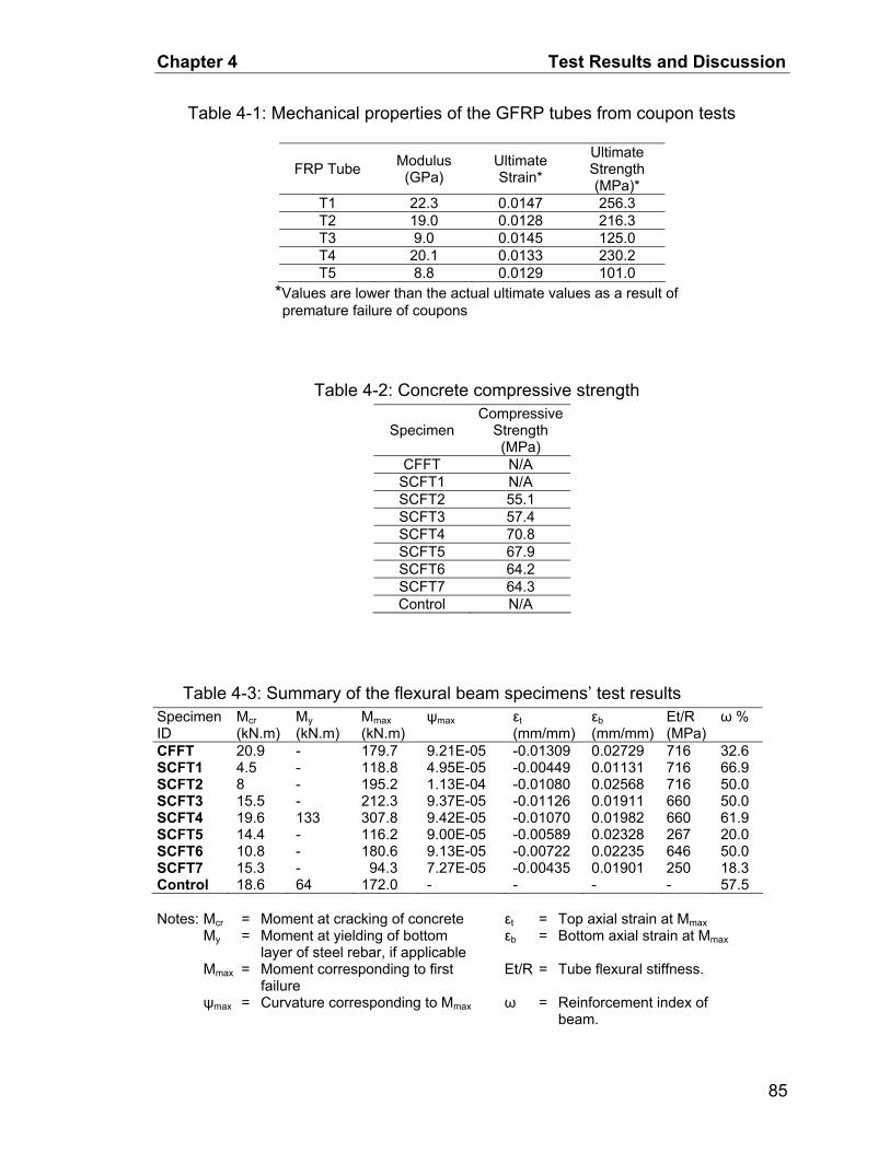
Chapter 4 Test Results and Discussion
Table 4-1: Mechanical properties of the GFRP tubes from coupon tests
FRP Tube Modulus (GPa)
Ultimate Strain*
Ultimate Strength (MPa)*
T1 22.3 0.0147 256.3 T2 19.0 0.0128 216.3 T3 9.0 0.0145 125.0 T4 20.1 0.0133 230.2 T5 8.8 0.0129 101.0
*Values are lower than the actual ultimate values as a result of premature failure of coupons
Table 4-2: Concrete compressive strength
Specimen Compressive
Strength (MPa)
CFFT N/A SCFT1 N/A SCFT2 55.1 SCFT3 57.4 SCFT4 70.8 SCFT5 67.9 SCFT6 64.2 SCFT7 64.3 Control N/A
Table 4-3: Summary of the flexural beam specimens’ test results Specimen ID
Mcr (kN.m)
My (kN.m)
Mmax (kN.m)
ψmax εt(mm/mm)
εb(mm/mm)
Et/R (MPa)
ω %
CFFT 20.9 - 179.7 9.21E-05 -0.01309 0.02729 716 32.6 SCFT1 4.5 - 118.8 4.95E-05 -0.00449 0.01131 716 66.9 SCFT2 8 - 195.2 1.13E-04 -0.01080 0.02568 716 50.0 SCFT3 15.5 - 212.3 9.37E-05 -0.01126 0.01911 660 50.0 SCFT4 19.6 133 307.8 9.42E-05 -0.01070 0.01982 660 61.9 SCFT5 14.4 - 116.2 9.00E-05 -0.00589 0.02328 267 20.0 SCFT6 10.8 - 180.6 9.13E-05 -0.00722 0.02235 646 50.0 SCFT7 15.3 - 94.3 7.27E-05 -0.00435 0.01901 250 18.3 Control 18.6 64 172.0 - - - - 57.5 Notes: Mcr = Moment at cracking of concrete εt = Top axial strain at Mmax My = Moment at yielding of bottom
layer of steel rebar, if applicable εb = Bottom axial strain at Mmax
Mmax = Moment corresponding to first failure
Et/R = Tube flexural stiffness.
ψmax = Curvature corresponding to Mmax ω = Reinforcement index of beam.
85

Chapter 4 Test Results and Discussion
0
50
100
150
200
250
300
350
0 5000 10000 15000 20000 25000 30000
T5 T3 T1
T2
Strain (×10-6)
Stre
ss (M
Pa)
T4
Figure 4-1: Longitudinal coupon tensile stress-strain curves.
0
100
200
300
400
500
600
700
0 0.05 0.1 0.15
Strain (mm/mm)
Stre
ss (M
Pa)
No. 10M Rebar
No. 15M Rebar
0.2
Figure 4-2: Stress-strain curves for steel rebar in axial tension [Adopted from
Cole 2005].
T1
T5
T3Ultimate tensile strains from beam tests
86
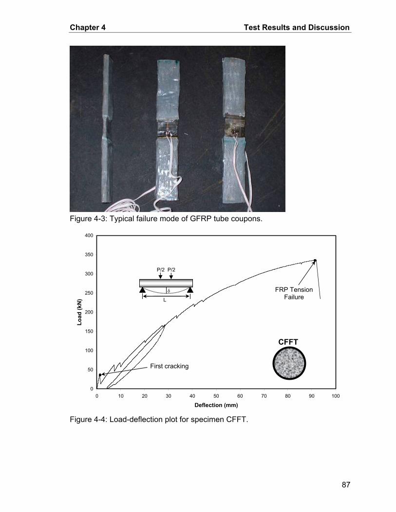
Chapter 4 Test Results and Discussion
Figure 4-3: Typical failure mode of GFRP tube coupons.
0
50
100
150
200
250
300
350
400
0 10 20 30 40 50 60 70 80 90 100
Deflection (mm)
Load
(kN
)
Figure 4-4: Load-deflection plot for specimen CFFT.
FRP Tension Failure
P/2 P/2
δ
L
First cracking
CFFT
87

Chapter 4 Test Results and Discussion
0
50
100
150
200
250
300
350
400
-20000 -15000 -10000 -5000 0 5000 10000 15000 20000 25000 30000 35000
Strain (×10-6)
Load
(kN
)
Figure 4-5: Longitudinal strain-load plot for specimen CFFT.
0
20
40
60
80
100
120
140
160
180
200
0 0.00001 0.00002 0.00003 0.00004 0.00005 0.00006 0.00007 0.00008 0.00009 0.0001
Curvature (rad/mm)
Mom
ent (
kN.m
)
Figure 4-6: Moment-curvature plot for specimen CFFT.
Top strain
Bottom strain
Tensile failure of the tube
88

Chapter 4 Test Results and Discussion
0
50
100
150
200
250
300
350
400
0 500 1000 1500 2000 2500 3000
Hoop Strain (×10-6)
Load
(kN
)
Figure 4-7: Load-hoop strain plot for specimen CFFT.
0
50
100
150
200
250
300
350
-4 -3.5 -3 -2.5 -2 -1.5 -1 -0.5 0
Slip (mm)
Load
(kN
)
End 2
End 1
Figure 4-8: Load-slip plot for specimen CFFT.
89

Chapter 4 Test Results and Discussion
Tube tensile Failure
Figure 4-9: Tensile failure of specimen CFFT.
0
50
100
150
200
250
0 10 20 30 40 50
Deflection (mm)
Load
(kN
)
Figure 4-10: Load-deflection plot for specimen SCFT1.
Crushing and spalling of concrete wall
P/2 P/2
δ First cracking
SCFT1
90

Chapter 4 Test Results and Discussion
0
50
100
150
200
250
-10000 -5000 0 5000 10000 15000 20000
Strain (×10-6)
Load
(kN
)
Crushing of Concrete
Top strain
Bottom strain
Figure 4-11: Load-longitudinal strain plot for specimen SCFT1.
0
20
40
60
80
100
120
140
0 0.00001 0.00002 0.00003 0.00004 0.00005 0.00006
Curvature (rad/mm)
Mom
ent (
kN.m
)
Figure 4-12: Moment-curvature plot for specimen SCFT1.
91
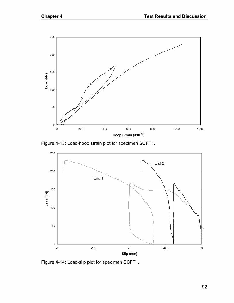
Chapter 4 Test Results and Discussion
0
50
100
150
200
250
0 200 400 600 800 1000 1200
Hoop Strain (Χ10-10)
Load
(kN
)
Figure 4-13: Load-hoop strain plot for specimen SCFT1.
0
50
100
150
200
250
-2 -1.5 -1 -0.5 0
Slip (mm)
Load
(kN
)
End 2
End 1
Figure 4-14: Load-slip plot for specimen SCFT1.
92
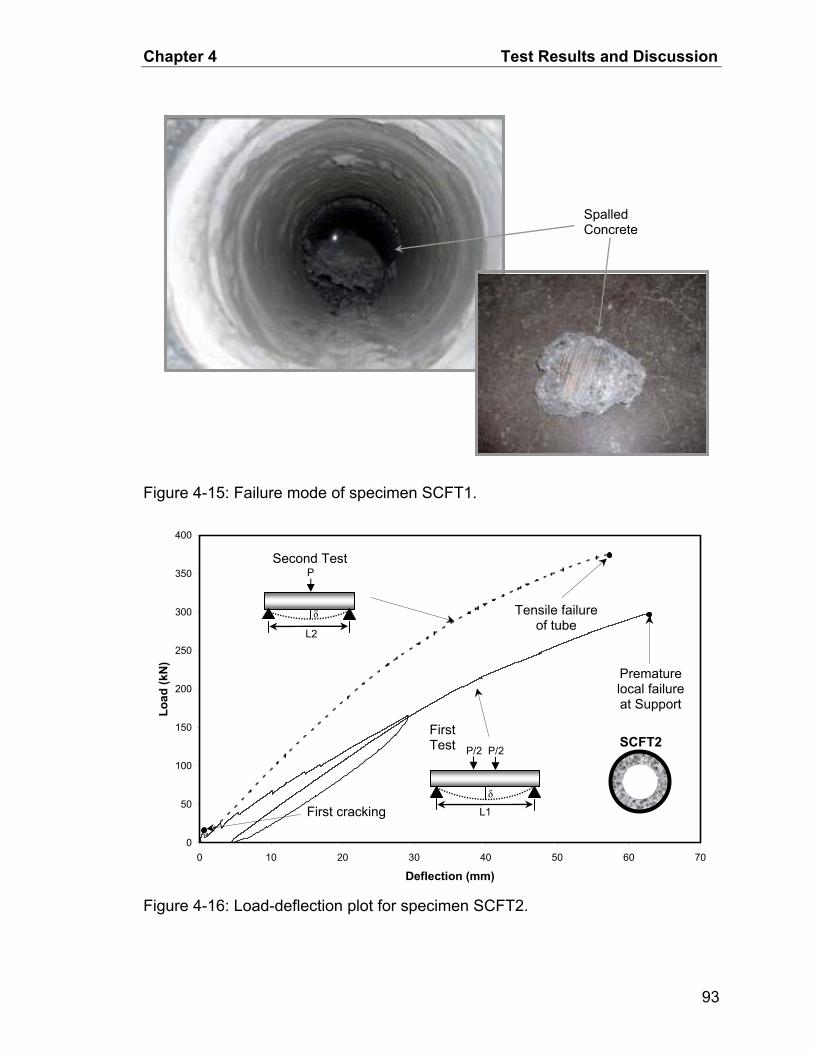
Chapter 4 Test Results and Discussion
Spalled Concrete
Figure 4-15: Failure mode of specimen SCFT1.
0
50
100
150
200
250
300
350
400
0 10 20 30 40 50 60 70
Deflection (mm)
Load
(kN
)
Figure 4-16: Load-deflection plot for specimen SCFT2.
L2
P
δ
Premature local failure at Support
P/2 P/2
δ
L1
SCFT2
First Test
Tensile failure of tube
Second Test
First cracking
93
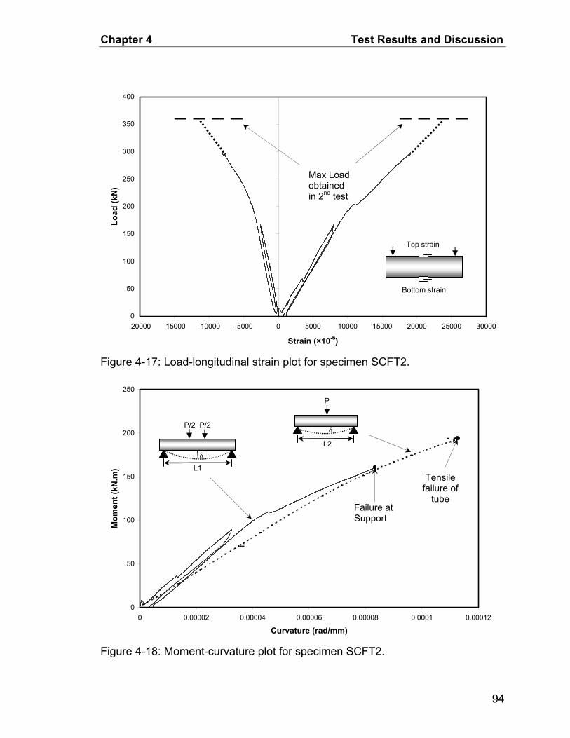
Chapter 4 Test Results and Discussion
0
50
100
150
200
250
300
350
400
-20000 -15000 -10000 -5000 0 5000 10000 15000 20000 25000 30000
Strain (×10-6)
Load
(kN
)
Top strain
Bottom strain
Max Load obtained in 2nd test
Figure 4-17: Load-longitudinal strain plot for specimen SCFT2.
0
50
100
150
200
250
0 0.00002 0.00004 0.00006 0.00008 0.0001 0.00012
Curvature (rad/mm)
Mom
ent (
kN.m
)
L2
P
Figure 4-18: Moment-curvature plot for specimen SCFT2.
δ
Failure at Support
P/2 P/2
δ L1
Tensile failure of
tube
94

Chapter 4 Test Results and Discussion
0
50
100
150
200
250
300
350
0 500 1000 1500 2000 2500
Hoop Strain (Χ10-6)
Load
(kN
)
Figure 4-19: Load-hoop strain plot for specimen SCFT2.
0
50
100
150
200
250
300
-3.5 -3 -2.5 -2 -1.5 -1 -0.5 0
Slip (mm)
Load
(kN
)
End 2
End 1
Figure 4-20: Load-slip plot for specimen SCFT2.
95

Chapter 4 Test Results and Discussion
Tube failure in tension at
midspan in sec-ond loading (3-point bending)
Premature failure at sup-
port in first loading (4-
point bending) due to defect
in tube
Figure 4-21: Failure mode of specimen SCFT2.
0
50
100
150
200
250
300
350
400
0 20 40 60 80 100 120 140 160 180 200
Deflection (mm)
Load
(kN
)
FRP failure progression
FRP Top compres-sion failure
First cracking FRP longitudinal tension failure
(Bottom)
SCFT3
L
δ
P
Figure 4-22: Load-deflection plot for specimen SCFT3.
96
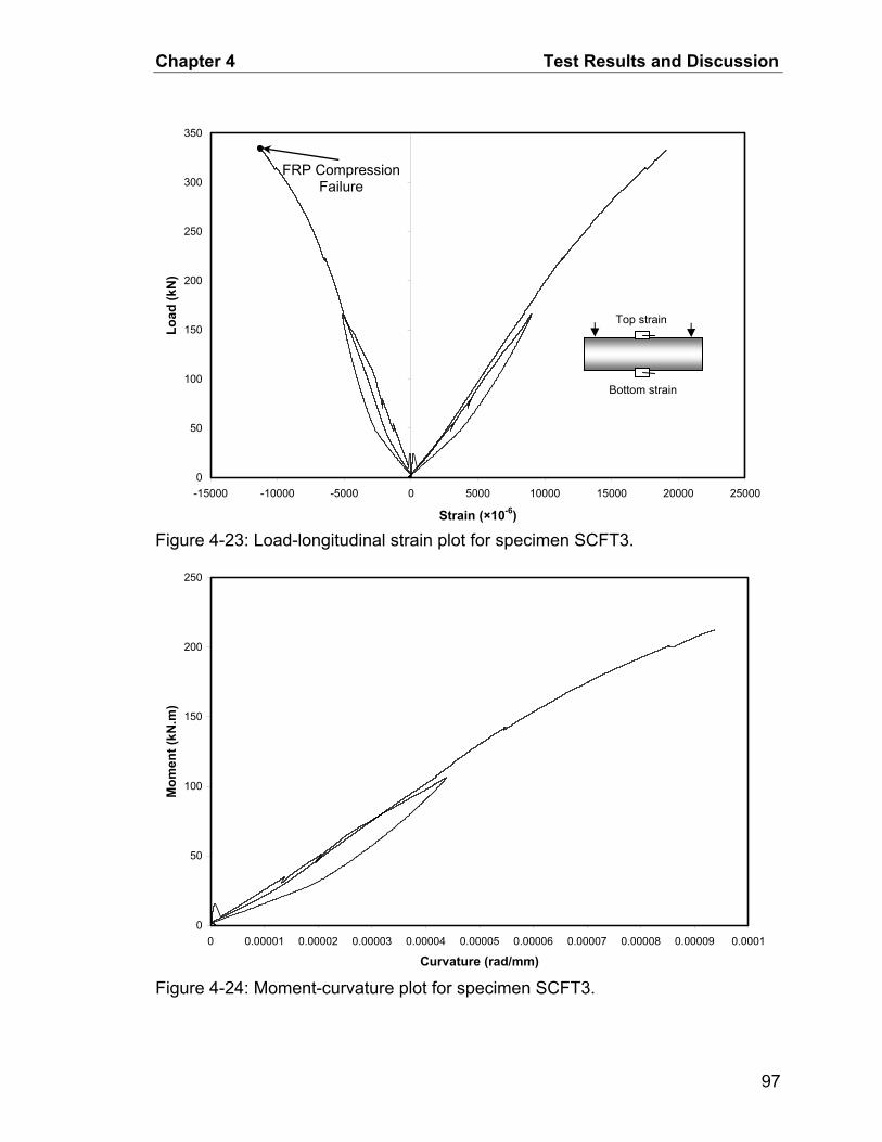
Chapter 4 Test Results and Discussion
0
50
100
150
200
250
300
350
-15000 -10000 -5000 0 5000 10000 15000 20000 25000
Strain (×10-6)
Load
(kN
)
FRP Compression Failure
Top strain
Bottom strain
Figure 4-23: Load-longitudinal strain plot for specimen SCFT3.
0
50
100
150
200
250
0 0.00001 0.00002 0.00003 0.00004 0.00005 0.00006 0.00007 0.00008 0.00009 0.0001
Curvature (rad/mm)
Mom
ent (
kN.m
)
Figure 4-24: Moment-curvature plot for specimen SCFT3.
97
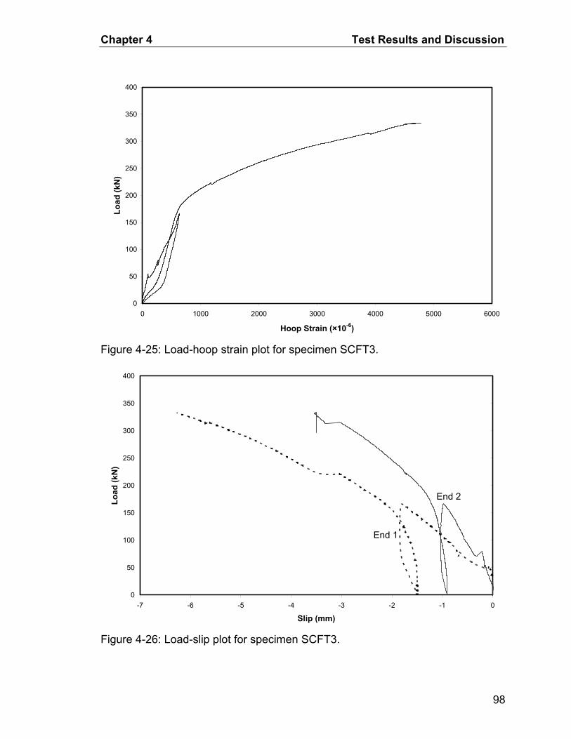
Chapter 4 Test Results and Discussion
0
50
100
150
200
250
300
350
400
0 1000 2000 3000 4000 5000 6000
Hoop Strain (×10-6)
Load
(kN
)
Figure 4-25: Load-hoop strain plot for specimen SCFT3.
0
50
100
150
200
250
300
350
400
-7 -6 -5 -4 -3 -2 -1 0
Slip (mm)
Load
(kN
)
End 2
End 1
Figure 4-26: Load-slip plot for specimen SCFT3.
98

Chapter 4 Test Results and Discussion
Compressive failure of FRP
tube
Figure 4-27: Failure mode of specimen SCFT3.
0
100
200
300
400
500
600
0 20 40 60 80 100
Compression failure of FRP tube
1
Load
(kN
)
20
Deflection (mm)
Figure 4-28: Load-deflection plot for specimen SCFT4.
FRP failure propagation
FRP hoop splitting
Yielding of bottom steel later
First cracking
SCFT4 L
δ
P
99

Chapter 4 Test Results and Discussion
0
100
200
300
400
500
600
-20000 -15000 -10000 -5000 0 5000 10000 15000 20000 25000
Strain (×10-6)
Load
(kN
)
Figure 4-29: Load-longitudinal strain plot for specimen SCFT4.
0
50
100
150
200
250
300
350
0 0.00001 0.00002 0.00003 0.00004 0.00005 0.00006 0.00007 0.00008 0.00009 0.0001
Curvature (rad/mm)
Mom
ent (
kN.m
)
Figure 4-30: Moment-curvature plot for specimen SCFT4.
Top strain
Bottom strain
FRP tube compres-sion Failure
100
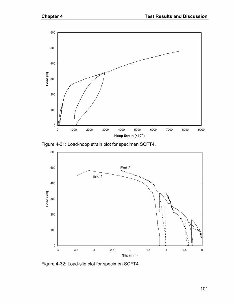
Chapter 4 Test Results and Discussion
0
100
200
300
400
500
600
0 1000 2000 3000 4000 5000 6000 7000 8000 9000
Hoop Strain (×10-6)
Load
(N)
Figure 4-31: Load-hoop strain plot for specimen SCFT4.
0
100
200
300
400
500
600
-4 -3.5 -3 -2.5 -2 -1.5 -1 -0.5 0
Slip (mm)
Load
(kN
)
End 2
End 1
Figure 4-32: Load-slip plot for specimen SCFT4.
101
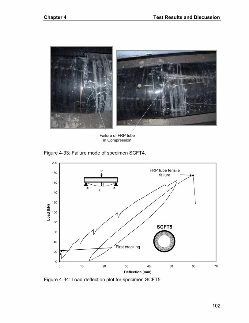
Chapter 4 Test Results and Discussion
Failure of FRP tube in Compression
Figure 4-33: Failure mode of specimen SCFT4.
0
20
40
60
80
100
120
140
160
180
200
0 10 20 30 40 50 60 7
Deflection (mm)
Load
(kN
)
0
Figure 4-34: Load-deflection plot for specimen SCFT5.
First cracking
FRP tube tensile failure
SCFT5
L
δ
P
102

Chapter 4 Test Results and Discussion
0
20
40
60
80
100
120
140
160
180
200
-10000 -5000 0 5000 10000 15000 20000 25000
Strain (×10-6)
Load
(kN
)
FRP tube tensile failure
Top strain
Bottom strain
Figure 4-35: Load-longitudinal strain plot for specimen SCFT5.
0
20
40
60
80
100
120
140
0 0.00001 0.00002 0.00003 0.00004 0.00005 0.00006 0.00007 0.00008 0.00009 0.0001
Curvature (rad/mm)
Mom
ent (
kN.m
)
Figure 4-36: Moment-curvature plot for specimen SCFT5.
103
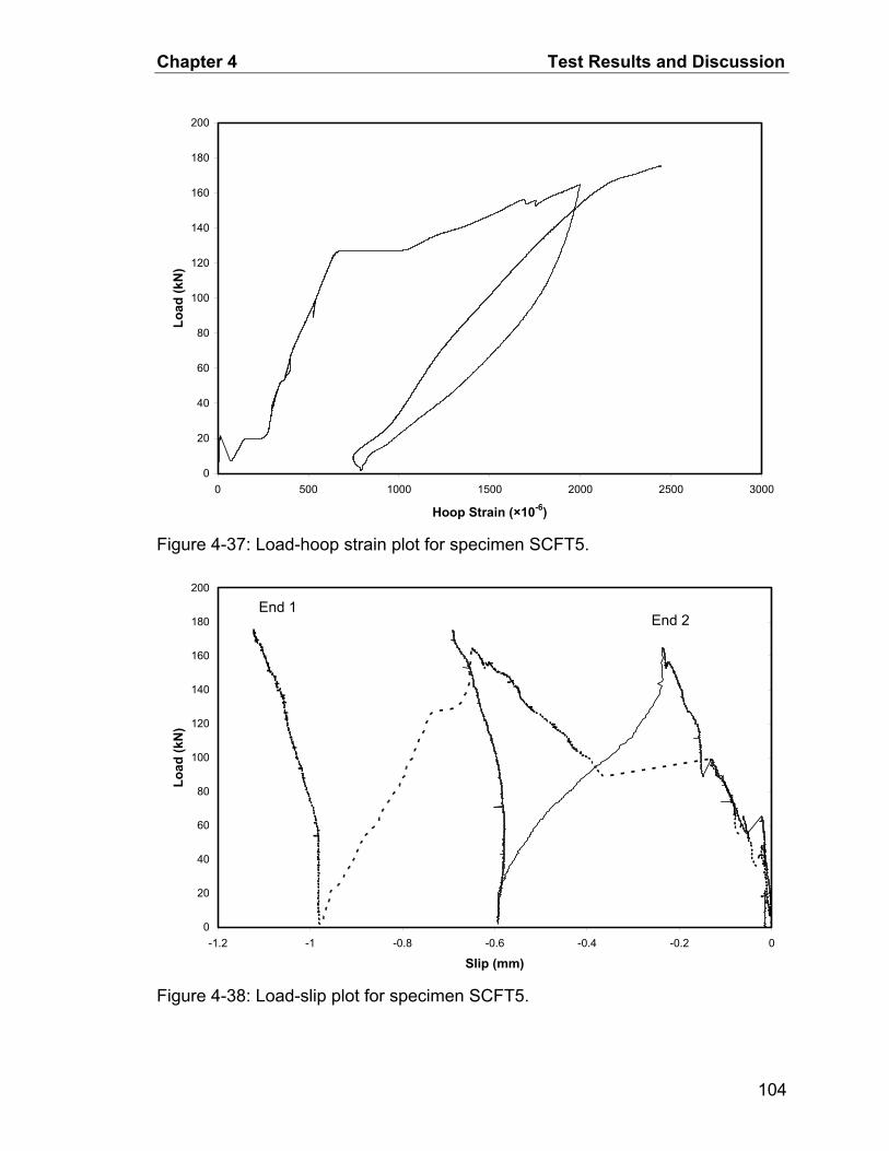
Chapter 4 Test Results and Discussion
0
20
40
60
80
100
120
140
160
180
200
0 500 1000 1500 2000 2500 3000
Hoop Strain (×10-6)
Load
(kN
)
Figure 4-37: Load-hoop strain plot for specimen SCFT5.
0
20
40
60
80
100
120
140
160
180
200
-1.2 -1 -0.8 -0.6 -0.4 -0.2 0
Slip (mm)
Load
(kN
)
End 2 End 1
Figure 4-38: Load-slip plot for specimen SCFT5.
104

Chapter 4 Test Results and Discussion
Tensile failure of FRP tube
Figure 4-39: Failure mode of specimen SCFT5.
0
50
100
150
200
250
300
0 20 40 60 80 100
Deflection (mm)120
Load
(kN
)
Figure 4-40: Load-deflection plot for specimen SCFT6.
First cracking
FRP tube com-pressive Failure
FRP hoop splitting
FRP tube failure propagation
SCFT6
L
δ
P
105

Chapter 4 Test Results and Discussion
0
50
100
150
200
250
300
-15000 -10000 -5000 0 5000 10000 15000 20000 25000
Strain (×10-6)
Load
(kN
)
FRP tube com-pression Failure
Top strain
Bottom strain
Figure 4-41: Load-longitudinal strain plot for specimen SCFT6.
0
20
40
60
80
100
120
140
160
180
200
0 0.00002 0.00004 0.00006 0.00008 0.0001 0.00012
Curvature (/mm)
Mom
ent (
kN.m
)
Figure 4-42: Moment-curvature plot for specimen SCFT6.
106

Chapter 4 Test Results and Discussion
0
50
100
150
200
250
300
0 1000 2000 3000 4000 5000 6000
Hoop Strain (×10-6)
Load
(kN
)
Figure 4-43: Load-hoop strain plot for specimen SCFT6.
0
50
100
150
200
250
300
-3 -2.5 -2 -1.5 -1 -0.5 0
Slip (mm)
Load
(kN
)
End 2 End 1
Figure 4-44: Load-slip plot for specimen SCFT6.
107
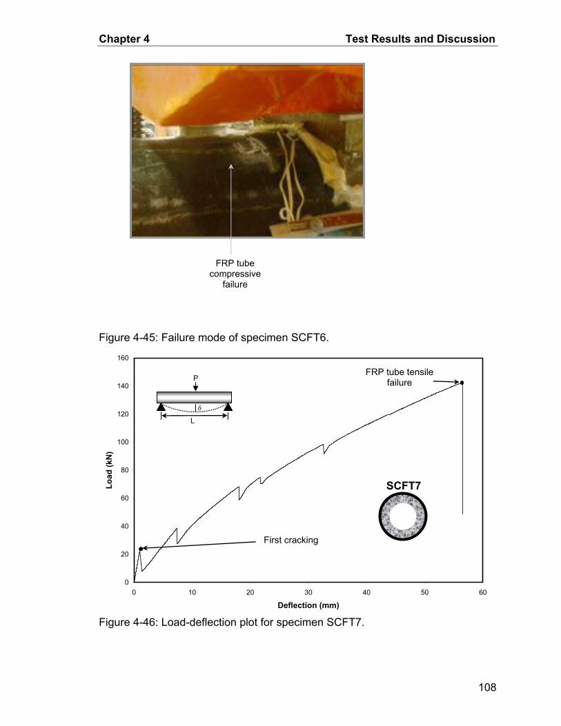
Chapter 4 Test Results and Discussion
FRP tube compressive
failure
Figure 4-45: Failure mode of specimen SCFT6.
0
20
40
60
80
100
120
140
160
0 10 20 30 40 50 6
Deflection (mm)
Load
(kN
)
FRP tube tensile failure
0
Figure 4-46: Load-deflection plot for specimen SCFT7.
First cracking
SCFT7
L
δ
P
108

Chapter 4 Test Results and Discussion
0
20
40
60
80
100
120
140
160
-10000 -5000 0 5000 10000 15000 20000 25000
Strain (×10-6)
Load
(kN
)
FRP tube tension failure
Top strain
Bottom strain
Figure 4-47: Load-longitudinal strain plot for specimen SCFT7.
0
10
20
30
40
50
60
70
80
90
100
0 0.00001 0.00002 0.00003 0.00004 0.00005 0.00006 0.00007 0.00008
Curvature (rad/mm)
Mom
ent (
kN.m
)
Figure 4-48: Moment-curvature plot for specimen SCFT7.
109

Chapter 4 Test Results and Discussion
0
20
40
60
80
100
120
140
160
0 200 400 600 800 1000 1200 1400 1600
Hoop Strain (×10-6)
Load
(kN
)
Figure 4-49: Load-hoop strain plot for specimen SCFT7.
0
20
40
60
80
100
120
140
160
-0.7 -0.6 -0.5 -0.4 -0.3 -0.2 -0.1 0
Slip (mm)
Load
(kN
)
End 2 End 1
Figure 4-50: Load slip plot for specimen SCFT7.
110

Chapter 4 Test Results and Discussion
Tensile failure of FRP tube
Figure 4-51: Failure mode of specimen SCFT7.
0
50
100
150
200
250
300
0 10 20 30 40 50 6
Deflection (mm)0
Load
(kN
)
Figure 4-52: Load-deflection plot of control specimen.
Secondary shear failure
Concrete crushing
Yielding of bottom steel
First cracking
L
δ
P
Control
111
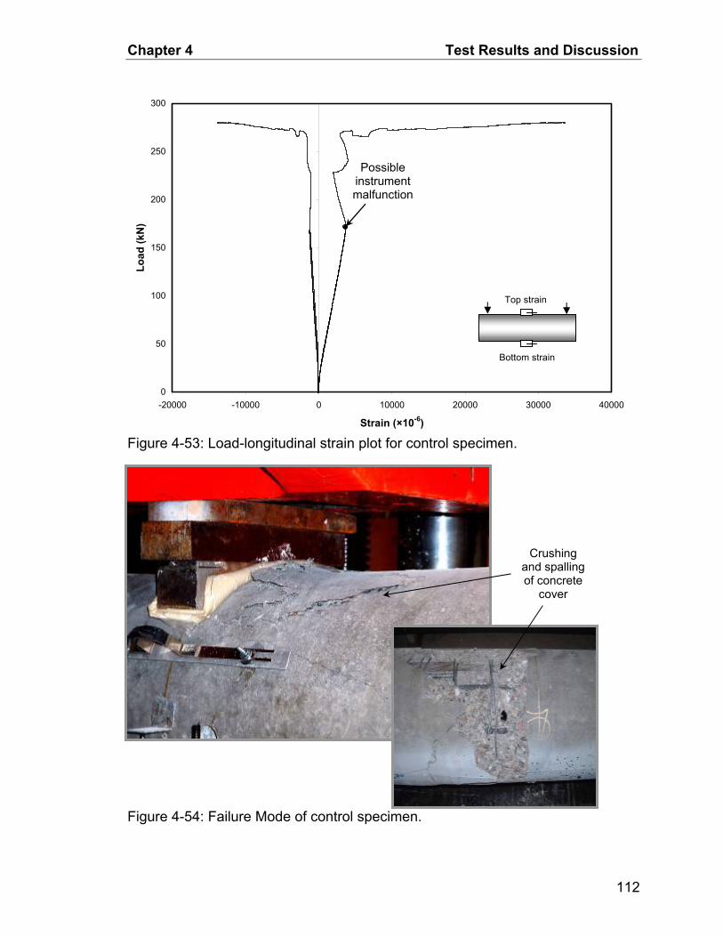
Chapter 4 Test Results and Discussion
0
50
100
150
200
250
300
-20000 -10000 0 10000 20000 30000 40000
Strain (×10-6)
Load
(kN
)
Possible instrument malfunction
Top strain
Bottom strain
Figure 4-53: Load-longitudinal strain plot for control specimen.
Figure 4-54: Failure Mode of control specimen.
Crushing and spalling of concrete
cover
112
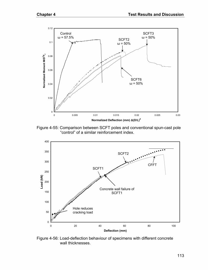
Chapter 4 Test Results and Discussion
0
0.02
0.04
0.06
0.08
0.1
0.12
0 0.005 0.01 0.015 0.02 0.025 0.03
Normalized Deflection (mm) Δ(D/L)4
Nor
mal
ized
Mom
ent M
/D3 f' c
Figure 4-55: Comparison between SCFT poles and conventional spun-cast pole “control” of a similar reinforcement index.
0
50
100
150
200
250
300
350
400
0 20 40 60 80 100
Deflection (mm)
Load
(kN
)
Figure 4-56: Load-deflection behaviour of specimens with different concrete wall thicknesses.
Concrete wall failure of SCFT1
Hole reduces cracking load
SCFT1
SCFT2
CFFT
Control ω = 57.5%
SCFT3 ω = 50% SCFT2
ω = 50%
SCFT6 ω = 50%
113
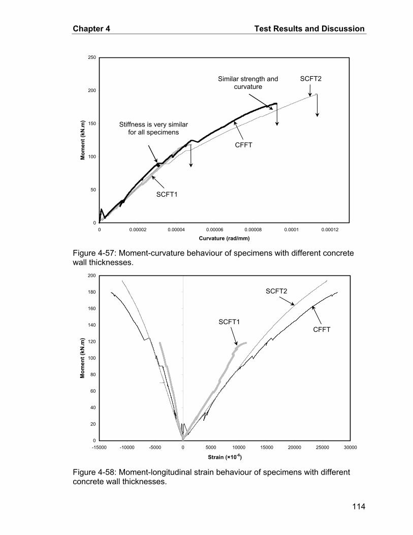
Chapter 4 Test Results and Discussion
0
50
100
150
200
250
SCFT2 Similar strength and curvature
0 0.00002 0.00004 0.00006 0.00008 0.0001 0.00012
Curvature (rad/mm)
Mom
ent (
kN.m
)
Stiffness is very similar for all specimens
Figure 4-57: Moment-curvature behaviour of specimens with different concrete wall thicknesses.
0
20
40
60
80
100
120
140
160
180
200
-15000 -10000 -5000 0 5000 10000 15000 20000 25000 30000
Strain (×10-6)
Mom
ent (
kN.m
)
Figure 4-58: Moment-longitudinal strain behaviour of specimens with different concrete wall thicknesses.
CFFT
SCFT1
SCFT1
SCFT2
CFFT
114
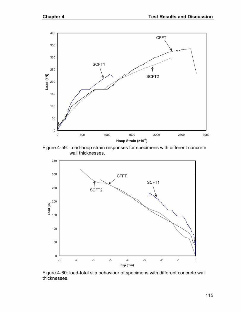
Chapter 4 Test Results and Discussion
0
50
100
150
200
250
300
350
400CFFT
SCFT1
0 500 1000 1500 2000 2500 3000
Hoop Strain (×10-6)
Load
(kN
)
SCFT2
Figure 4-59: Load-hoop strain responses for specimens with different concrete wall thicknesses.
0
50
100
150
200
250
300
350
-8 -7 -6 -5 -4 -3 -2 -1 0
Slip (mm)
Load
(kN
)
SCFT1
SCFT2
CFFT
Figure 4-60: load-total slip behaviour of specimens with different concrete wall thicknesses.
115
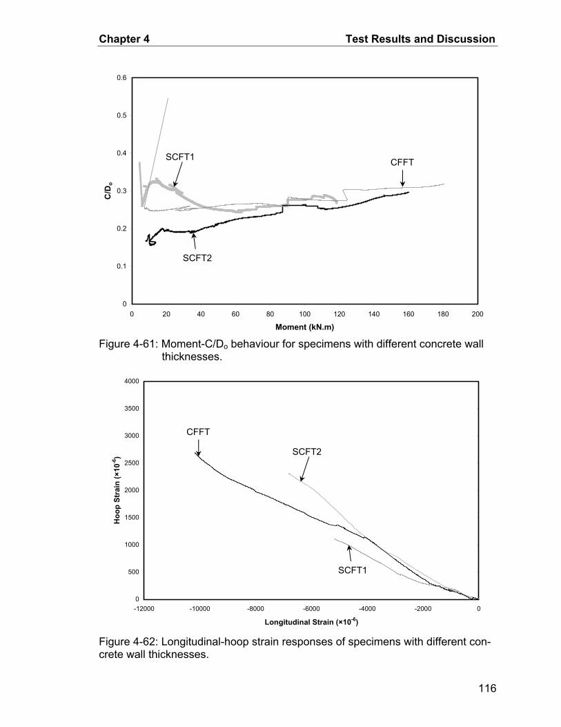
Chapter 4 Test Results and Discussion
0
0.1
0.2
0.3
0.4
0.5
0.6
0 20 40 60 80 100 120 140 160 180 200
Moment (kN.m)
C/D
o
Figure 4-61: Moment-C/Do behaviour for specimens with different concrete wall thicknesses.
0
500
1000
1500
2000
2500
3000
3500
4000
-12000 -10000 -8000 -6000 -4000 -2000 0
Longitudinal Strain (×10-6)
Hoo
p St
rain
(×10
-6)
Figure 4-62: Longitudinal-hoop strain responses of specimens with different con-crete wall thicknesses.
SCFT1 CFFT
SCFT2
SCFT2
SCFT1
CFFT
116

Chapter 4 Test Results and Discussion
0
0.2
0.4
0.6
0.8
1
1.2
0 0.1 0.2 0.3 0.4 0.5 0.6 0.7 0.8
Di/Do
Mu/
Mu f
ull
Figure 4-63: Variation of normalized flexural strength with inner-to-outer diameter ratio.
0
20
40
60
80
100
120
0 0.1 0.2 0.3 0.4 0.5 0.6 0.7 0
Di/Do.8
SCFT2
SCFT1
CFFT
SCFT2
SCFT1
CFFT
Pu/W
Figure 4-64: Variation of flexural strength-to-weight ratio with inner-to-outer di-ameter ratio.
117
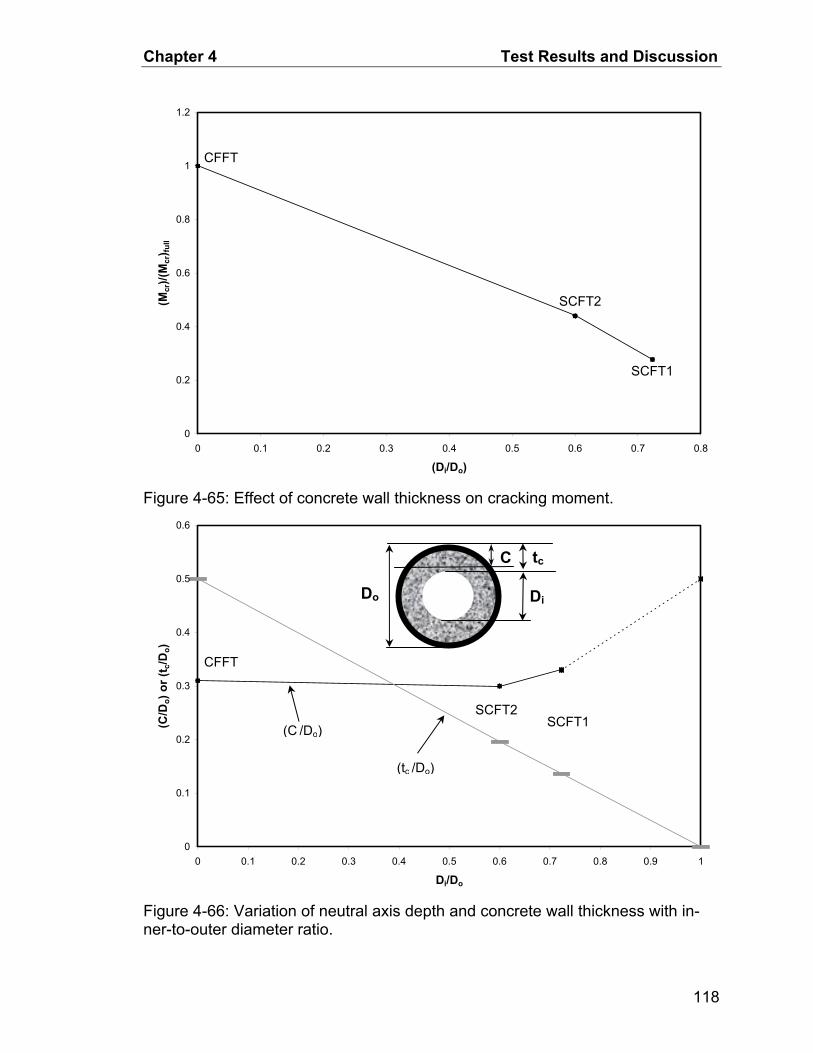
Chapter 4 Test Results and Discussion
0
0.2
0.4
0.6
0.8
1
1.2
0 0.1 0.2 0.3 0.4 0.5 0.6 0.7 0.8
(Di/Do)
(Mcr
)/(M
cr) fu
ll
SCFT2
SCFT1
CFFT
Figure 4-65: Effect of concrete wall thickness on cracking moment.
0
0.1
0.2
0.3
0.4
0.5
0.6
0 0.1 0.2 0.3 0.4 0.5 0.6 0.7 0.8 0.9 1
Di/Do
(C/D
o) o
r (t c
/Do)
tc
Di
C
Do
(tc /Do)
SCFT2 SCFT1
CFFT
(C /Do)
Figure 4-66: Variation of neutral axis depth and concrete wall thickness with in-ner-to-outer diameter ratio.
118

Chapter 4 Test Results and Discussion
0
100
200
300
400
500
600
0 20 40 60 80 100 120 140 160 180 200
Increase in strength due to
rebar
Deflection (mm)
Load
(kN
)
Figure 4-67: Effect of longitudinal steel reinforcement on responses of SCFT3 and SCFT4.
0
100
200
300
400
500
600
-12 -10 -8 -6 -4 -2 0
Slip (mm)
Load
(kN
)
Figure 4-68: Load-slip response comparison between SCFT3 and SCFT4.
Hoop splitting of tube
SCFT4 SCFT3
Slip reduction due to rebar.
SCFT4
SCFT3
119

Chapter 4 Test Results and Discussion
0
1000
2000
3000
4000
5000
6000
7000
8000
9000
Significant increase in confinement
-12000 -10000 -8000 -6000 -4000 -2000 0
Longitudinal Strain (×10-6)
Hoo
p St
rain
(×10
-6)
SCFT4
SCFT3
Figure 4-69: Variation of hoop strains with longitudinal strains in compression in specimens.
0
50
100
150
200
250
300
350
0 0.00002 0.00004 0.00006 0.00008 0.0001 0.00012
Curvature (rad/mm)
Mom
ent (
kN.m
)
SCFT4
SCFT3
Figure 4-70: Moment-curvature plots of specimens SCFT3 and SCFT4.
120
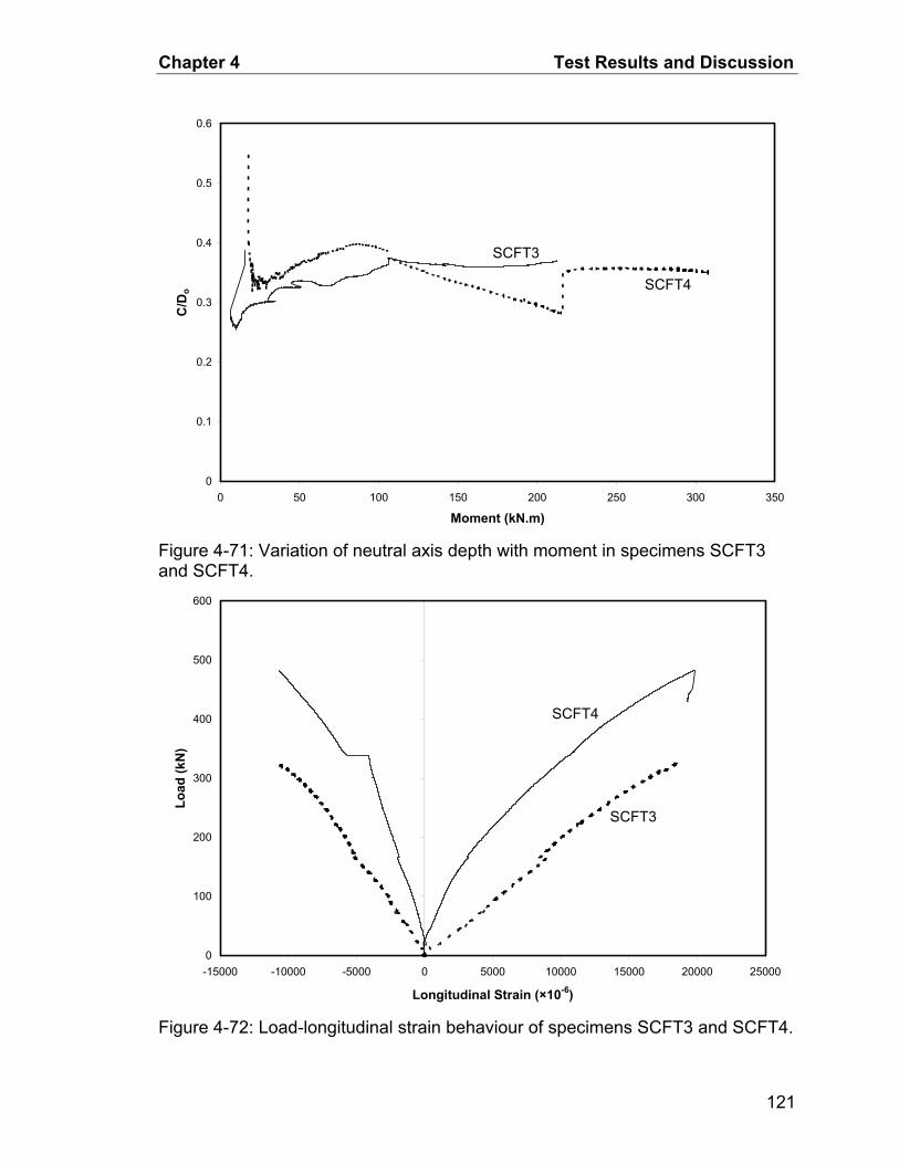
Chapter 4 Test Results and Discussion
0
0.1
0.2
0.3
0.4
0.5
0.6
0 50 100 150 200 250 300 350
Moment (kN.m)
C/D
o
SCFT4
SCFT3
Figure 4-71: Variation of neutral axis depth with moment in specimens SCFT3 and SCFT4.
0
100
200
300
400
500
600
-15000 -10000 -5000 0 5000 10000 15000 20000 25000
Longitudinal Strain (×10-6)
Load
(kN
)
SCFT4
SCFT3
Figure 4-72: Load-longitudinal strain behaviour of specimens SCFT3 and SCFT4.
121

Chapter 4 Test Results and Discussion
0
100
200
300
400
500
600
0 1000 2000 3000 4000 5000 6000 7000 8000 9000
Hoop Strain (×10-6)
Load
(kN
)
SCFT4
SCFT3
Figure 4-73: Load-hoop strain behaviour of specimens SCFT3 and SCFT4.
0
50
100
150
200
250
0 0.00002 0.00004 0.00006 0.00008 0.0001 0.00012
Curvature (rad/mm)
Mom
ent (
kN.m
)
SCFT6
SCFT3 SCFT2
SCFT7
SCFT5
Figure 4-74: Moment-curvature plots of SCFT specimens of different tubes.
122

Chapter 4 Test Results and Discussion
0
1000
2000
3000
4000
5000
6000
-8000 -7000 -6000 -5000 -4000 -3000 -2000 -1000 0
Longitudinal Strain (×10-6)
Hoo
p St
rain
(×10
-6)
Figure 4-75: Hoop-longitudinal strain comparison between SCFT6 and SCFT2.
0
50
100
150
200
250
300
-6 -5 -4 -3 -2 -1 0
Slip (mm)
Load
(kN
)
Figure 4-76: Load-slip responses of SCFT6 and SCFT2.
123

Chapter 4 Test Results and Discussion
0
0.05
0.1
0.15
0.2
0.25
0 5 10 15 20 25 30 35 40 45 50
Slip (mm)
Stre
ss (M
Pa)
S1S2S3
Figure 4-77: Bond stress vs. slip for short push-off specimens.
0
0.05
0.1
0.15
0.2
0.25
0 5 10 15 20 25 30 35 40 45 50
Slip (mm)
Stes
s (M
Pa)
L1L2L3
Figure 4-78: Bond stress vs. slip for long push-off specimens.
Specimen cut from end of the Tube
Specimen cut from end of the Tube
Concrete
Tube
8 mm
124
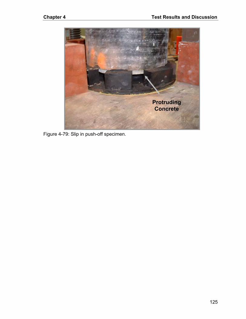
Chapter 4 Test Results and Discussion
Figure 4-79: Slip in push-off specimen.
Protruding Concrete
125

Chapter 5 Analytical Modeling of SCFTs
CHAPTER 5 : ANALYTICAL MODELLING OF SCFTS
Introduction
This chapter describes an analytical model that has been developed to predict
the flexural behaviour of spun-cast concrete-filled FRP tubes (SCFTs). The flex-
ural model presented extends the model developed by Fam (2000) for CFFTs by
including the central hole in SCFTs, and accounts for the slight non-linearity of
the FRP tube arising from progressive laminate failure. It is based on strain
compatibility, internal force equilibrium, and material constitutive relationships,
which also account for concrete non-linearity. The GFRP tube material proper-
ties are determined using coupon test results and were also predicted using the
Classical Lamination Theory (CLT), which incorporates the Ultimate Laminate
Failure (CLT-ULF) approach. The CLT-ULF approach accounts for progressive
failure of the individual layers oriented at different angles in the laminate. After
verifying the model using the experimental results, a detailed parametric study
was carried out to determine the effects of tube thickness, laminate structure and
concrete wall thickness on the flexural behaviour of SCFTs.
Analytical Model for SCFTs in Flexure
In the following sections, the analytical model used to predict the complete
behaviour of SCFT specimens in flexure is explained, verified against experimen-
tal results, and a parametric study on the flexural behaviour of SCFTs is also pre-
sented.
126
Chapter 5 Analytical Modeling of SCFTs
Description of the Analytical Model
The model is based on the assumption that plane sections remain plane after
deformation, which indicates linear strain distribution over the depth of SCFTs
subjected to bending. Also, no slip is assumed to occur between the GFRP tube
and the concrete, so that the strain compatibility assumption is valid. This as-
sumption is reasonable based on the very small slip observed in the flexural
tests. The model accounts for nonlinearities in the concrete and the GFRP tube.
A layer-by-layer approach is adopted to sum the forces and moments over the
cross-sectional depth.
Section Geometry
The geometry of a circular section is more complex than that of a rectangular
one. The stresses, which are variable over the section depth, are also distributed
along an area of variable width. In addition, the reinforcement (i.e. the GFRP
tube) is continuous around the perimeter, such that the cross-sectional area of
reinforcement at any given depth is more difficult to calculate than in conventional
reinforced concrete sections. In order to integrate the stresses over the cross-
sectional area, a layer-by-layer approach has been adopted. The actual geometry
of the SCFT, shown in Figure 5-1(a), is idealized into discrete layers, as shown in
Figure 5-5(b). The depth of the tube, D, is taken as the diameter based on the
average thickness of the tube, given by:
OD D t= − (5-1)
Where Do is the outer diameter of the tube and t is the structural thickness of
the tube. The depth D is divided into a number of layers, n, of equal thickness, hi.
127
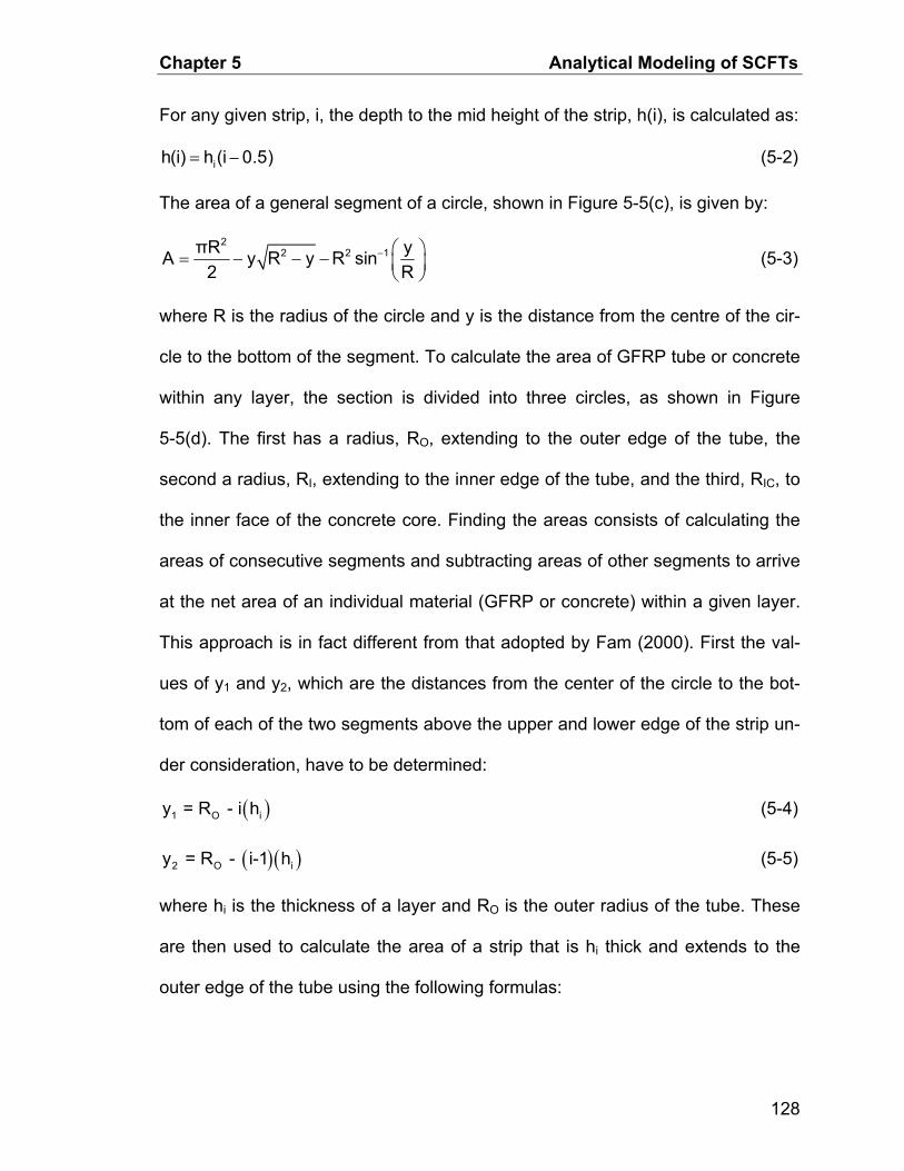
Chapter 5 Analytical Modeling of SCFTs
For any given strip, i, the depth to the mid height of the strip, h(i), is calculated as:
ih(i) h (i 0.5)= − (5-2)
The area of a general segment of a circle, shown in Figure 5-5(c), is given by:
22 2 1πRA y R y R sin
2 R− ⎛ ⎞= − − − ⎜ ⎟⎝ ⎠
y
i
(5-3)
where R is the radius of the circle and y is the distance from the centre of the cir-
cle to the bottom of the segment. To calculate the area of GFRP tube or concrete
within any layer, the section is divided into three circles, as shown in Figure
5-5(d). The first has a radius, RO, extending to the outer edge of the tube, the
second a radius, RI, extending to the inner edge of the tube, and the third, RIC, to
the inner face of the concrete core. Finding the areas consists of calculating the
areas of consecutive segments and subtracting areas of other segments to arrive
at the net area of an individual material (GFRP or concrete) within a given layer.
This approach is in fact different from that adopted by Fam (2000). First the val-
ues of y1 and y2, which are the distances from the center of the circle to the bot-
tom of each of the two segments above the upper and lower edge of the strip un-
der consideration, have to be determined:
( )1 O iy = R - i h (5-4)
( )( )2 Oy = R - i-1 h (5-5)
where hi is the thickness of a layer and RO is the outer radius of the tube. These
are then used to calculate the area of a strip that is hi thick and extends to the
outer edge of the tube using the following formulas:
128

Chapter 5 Analytical Modeling of SCFTs
22 2 1O 1
O1 1 O 1 OO
πR yA y R y R sin2 R
− ⎛ ⎞= − − − ⎜
⎝ ⎠⎟ (5-6)
and,
22 2 1O 2
O2 2 O 2 OO
πR yA y R y R sin2 R
− ⎛ ⎞= − − − ⎜
⎝ ⎠⎟
2
(5-7)
The net area of the strip, AO is:
O O1 OA A A= − (5-8)
Next, the calculation is repeated for consecutive segments having a radius ex-
tending to the inner face of the tube:
22 2 1I
C1 1 I 1 II
πRA y R y R sin2 R
− ⎛ ⎞= − − − ⎜ ⎟
⎝ ⎠1y (5-9)
and,
22 2 1I
C2 2 I 2 II
πRA y R y R sin2 R
− ⎛ ⎞= − − − ⎜
⎝ ⎠2y⎟
C2
(5-10)
The net area of the strip, AC, is:
C C1A A A= − (5-11)
and the net area of the GFRP tube for this strip is:
( )F Oi CA A A= − (5-12)
Finally, two consecutive segments extending to the inner face of the concrete are
calculated using the same procedure:
22 2 1IC 1
H1 1 IC 1 ICIC
πR yA y R y R sin2 R
− ⎛ ⎞= − − − ⎜
⎝ ⎠⎟ (5-13)
and,
129
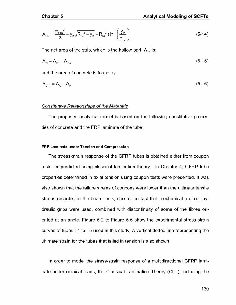
Chapter 5 Analytical Modeling of SCFTs
22 2 1RIC 2
H2 2 IC 2 ICIC
π yA y R y R sin2 R
− ⎛ ⎞= − − − ⎜
⎝ ⎠⎟
2
(5-14)
The net area of the strip, which is the hollow part, AH, is:
H H1 HA A A= − (5-15)
and the area of concrete is found by:
( )C Ci HA A A= − (5-16)
Constitutive Relationships of the Materials
The proposed analytical model is based on the following constitutive proper-
ties of concrete and the FRP laminate of the tube.
FRP Laminate under Tension and Compression
The stress-strain response of the GFRP tubes is obtained either from coupon
tests, or predicted using classical lamination theory. In Chapter 4, GFRP tube
properties determined in axial tension using coupon tests were presented. It was
also shown that the failure strains of coupons were lower than the ultimate tensile
strains recorded in the beam tests, due to the fact that mechanical and not hy-
draulic grips were used, combined with discontinuity of some of the fibres ori-
ented at an angle. Figure 5-2 to Figure 5-6 show the experimental stress-strain
curves of tubes T1 to T5 used in this study. A vertical dotted line representing the
ultimate strain for the tubes that failed in tension is also shown.
In order to model the stress-strain response of a multidirectional GFRP lami-
nate under uniaxial loads, the Classical Lamination Theory (CLT), including the
130

Chapter 5 Analytical Modeling of SCFTs
Ultimate Laminate Failure (CLT-ULF) approach, which assumes that the laminate
does not fail until all fibre layers have failed, has been adopted. Details about the
various assumptions involved and detailed derivations pertaining to CLT-ULF can
be found in Daniel and Ishai (1994). In this study, a spreadsheet that is readily
available has been used for predictions. Figure 5-2 to Figure 5-6 show the pre-
dicted stress-strain responses of the GFRP tubes. Values at key points on the
curves were also summarized in Chapter 3 (Table 3.1) and compared to the ex-
perimental values. As shown in the Figures, good agreement is generally ob-
served, however, predictions also tended to show a failure strain of about 0.0155,
which is short of the ultimate tensile strain recorded during the beam tests. This is
attributed to the fact that the CLT treats both the fibres and resins as linear elastic
materials, whereas the nonlinear stress-strain response of the tube could be ex-
plained by the progressive failure of the laminate structure, combined with the
non-linearity of the resin.
In order to overcome this problem, a survey of failure strains of similar tubes
fabricated by the same manufacturer was conducted from the literature. The sur-
vey included CFFT beams tested by Fam (2000), Mandal (2004), Cole (2005)
and the current study. The tubes ranged in diameter from 89 mm to 326 mm and
in thickness from 2.05 mm to 6.4 mm. They also varied in laminate structure,
such that the axial and hoop modulii varied from about 15 GPa to 31 GPa. Figure
5-7 shows the failure strain of all the tubes plotted against a parameter, ω’, which
represents the tube diameter-to thickness ratio (D/t) and axial-to-hoop modulus
ratio (Eaxial/Ehoop) as given in Equation 5-17:
131

Chapter 5 Analytical Modeling of SCFTs
axial
hoop
E Dω E⎛ ⎞⎛ ⎞⎜ ⎟⎜ ⎟⎜ ⎟⎜ ⎟⎝ ⎠⎝ ⎠
=′ t (5-17)
Figure 5-7 shows that strains at failure varied from 0.0154 to 0.028, with most
values very close to the average of 0.022. As such this value of 0.022 is consid-
ered the limiting value in analysis. A second order polynomial is used to fit the
four points obtained from the Classical Lamination Theory on the predicted
stress-strain curve, and then the polynomial is extended to the 0.022 strain as
shown in Figure 5-2 to Figure 5-6. As for the behaviour of the tubes in compres-
sion, Mandal (2004) has shown that, for filament-wound GFRP tubes similar to
those used in this study, the stress-strain curves in axial tension and compres-
sion are quite similar. Thus it was assumed that behaviour of the tube was identi-
cal in both tension and compression.
Concrete under Tension and Compression
Fam and Rizkalla (2002) have shown that for circular SCFTs with no internal
reinforcement, loaded in bending, concrete in the compression zone exhibits ex-
tended strain softening due to the very low (partial) confinement. Two concrete
models are used in compression. The first model is the unconfined concrete
model, by Popovics (1973), with extended strain-softening. As shown in Figure
5-8(a), the compressive stress fc, corresponding to strain cε , is given by:
( )( )
c c cc r
c c
f ε / ε rf
r 1 ε / ε
′ ′=
′− + (5-18)
where is the unconfined concrete strength, cf ′ cε ′ is the corresponding strain,
132
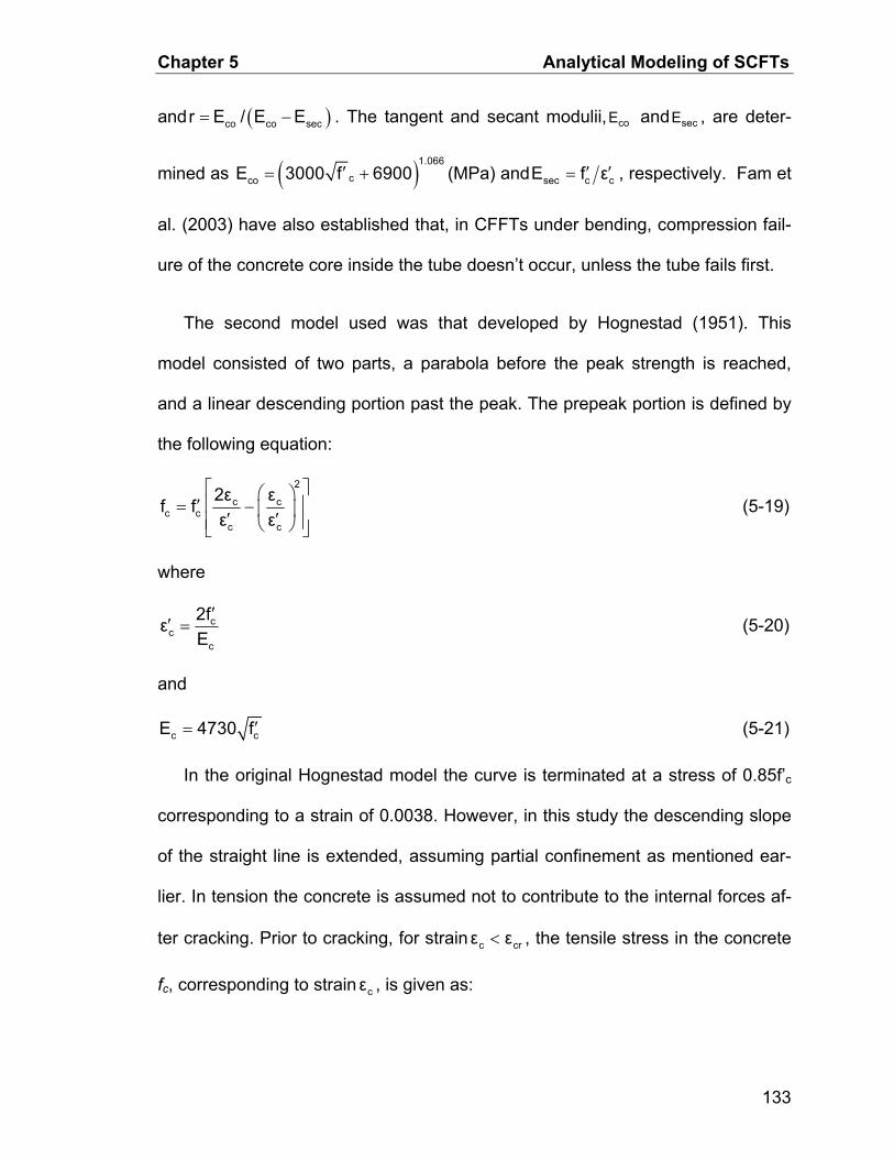
Chapter 5 Analytical Modeling of SCFTs
and . The tangent and secant modulii, and , are deter-
mined as
(co co secr E / E E= − ) coE secE
( )1.066
ccoE 3000 f 6900′= + (MPa) and sec c cE f ε′ ′= , respectively. Fam et
al. (2003) have also established that, in CFFTs under bending, compression fail-
ure of the concrete core inside the tube doesn’t occur, unless the tube fails first.
The second model used was that developed by Hognestad (1951). This
model consisted of two parts, a parabola before the peak strength is reached,
and a linear descending portion past the peak. The prepeak portion is defined by
the following equation:
2
c cc c
c c
2ε εf fε ε
⎡ ⎤⎛ ⎞′ ⎢= − ⎜ ⎟′ ′⎢ ⎥⎝ ⎠⎣ ⎦
⎥ (5-19)
where
cc
c
2fεE′
′ = (5-20)
and
cE 4730 f ′= c
cr
(5-21)
In the original Hognestad model the curve is terminated at a stress of 0.85f’c
corresponding to a strain of 0.0038. However, in this study the descending slope
of the straight line is extended, assuming partial confinement as mentioned ear-
lier. In tension the concrete is assumed not to contribute to the internal forces af-
ter cracking. Prior to cracking, for strain cε ε< , the tensile stress in the concrete
fc, corresponding to strain , is given as: cε
133
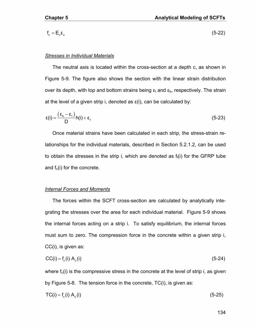
Chapter 5 Analytical Modeling of SCFTs
(5-22) c cf E ε= c
Stresses in Individual Materials
The neutral axis is located within the cross-section at a depth c, as shown in
Figure 5-9. The figure also shows the section with the linear strain distribution
over its depth, with top and bottom strains being εt and εb, respectively. The strain
at the level of a given strip i, denoted as ε(i), can be calculated by:
( )b tt
ε εε(i) h(i) ε
D−
= + (5-23)
Once material strains have been calculated in each strip, the stress-strain re-
lationships for the individual materials, described in Section 5.2.1.2, can be used
to obtain the stresses in the strip i, which are denoted as ff(i) for the GFRP tube
and fc(i) for the concrete.
Internal Forces and Moments
The forces within the SCFT cross-section are calculated by analytically inte-
grating the stresses over the area for each individual material. Figure 5-9 shows
the internal forces acting on a strip i. To satisfy equilibrium, the internal forces
must sum to zero. The compression force in the concrete within a given strip i,
CC(i), is given as:
c cCC(i) f (i) A (i)= (5-24)
where fc(i) is the compressive stress in the concrete at the level of strip i, as given
by Figure 5-8. The tension force in the concrete, TC(i), is given as:
c cTC(i) f (i) A (i)= (5-25)
134

Chapter 5 Analytical Modeling of SCFTs
where fc(i) is the tensile stress in the concrete, given in Equation (5-12). The
compression and tension forces in the FRP tube at a given strip i, denoted as
CF(i) and TF(i), respectively, are:
f fCF(i) f (i) A (i)= (5-26)
f fTF(i) f (i) A (i)= (5-27)
where ff(i) is the FRP tube compressive or tensile stress, obtained from the sec-
ond order polynomial in Figure 5-2 to Figure 5-6. The total compressive forces in
the concrete, CCC, and the FRP tube, CFF, are the sum of the negative forces
acting on all strips of the cross section, given as:
i n
i 0CCC CC(i) when CC(i) < 0
=
=
= ∑ (5-28)
i n
i 0CFF CF(i) when CF(i) < 0
=
=
= ∑ (5-29)
The total tension forces in the concrete, TCC, and the FRP tube, TFF, are the
sum of the forces acting on all strips located below the neutral axis, given as:
i n
i 0TCC TC(i) when TC(i) > 0
=
=
= ∑ (5-30)
i n
i 0TFF TF(i) when TF(i) > 0
=
=
= ∑ (5-31)
For equilibrium of forces, the sum of all compression and tension forces must
satisfy the condition:
CCC CFF TCC TFF 0+ + + = (5-32)
The internal moment is only calculated when equilibrium is satisfied. The total
moments due to the compression and tension forces in the concrete, and FRP
135
Chapter 5 Analytical Modeling of SCFTs
tube are calculated from the following equations:
i n
i 0MCC CC(i) h(i) when CC(i) < 0
=
=
= ∑ (5-33)
i n
i 0MTC TC(i) h(i) when TC(i) > 0
=
=
= ∑ (5-34)
i n
i 0MCF CF(i) h(i) when CF(i) < 0
=
=
= ∑ (5-35)
i n
i 0MTF TF(i) h(i) when TF(i) > 0
=
=
= ∑ (5-36)
where MCC is the moment for concrete in compression, MTC is the moment for
concrete in tension, MCF is the moment for the FRP tube in compression, MTF is
the moment for the FRP tube in tension, and h(i) is the distances from the top
fibre of the section to the mid-height of layer i. The total moment is the sum of the
internal moments as follows:
MOMENT MCC MCF MTC MTF= + + + (5-37)
The corresponding curvature of the section, ψ, which is the slope of the strain
profile, is calculated as:
tεψc
= (5-38)
where εt is the compressive strain of the top fibre of the tube.
Failure Criteria
Failure at ultimate refers to the first failure taking place in the SCFT system
when either the extreme tension or extreme compression FRP fibres reach the
ultimate strain. As the model was also used in a parametric study that involved a
136

Chapter 5 Analytical Modeling of SCFTs
lower bound case of a hollow FRP tube without any concrete, another failure cri-
terion was taken into account, namely buckling of the tube. The critical buckling
moment of the tube was found using the following equation (Ibrahim, 2000):
xxycrt
y
D4 2M πE RtE t3 3= × (5-39)
where t and R are the wall thickness and the original radius of the tube, Ey, is the
effective modulus in the circumferential direction of the composite laminate, and
Dxx is the circumferential bending stiffness of the tube calculated using the lami-
nation theory [Daniel and Ishai, 1994].
Procedure of Analysis
A computer program was developed using Fortran90 to generate the moment-
curvature response of SCFTs. The flowchart of the analytical model used to pre-
dict this response is shown in Figure 5-10, using the preceding equations. The
program code itself is given in Appendix A. The procedure can be summarized as
follows:
1. Specify tube diameter, thickness, material properties and number of layers.
2. Assume a value for compressive strain εt in the extreme top fibre of the FRP
tube.
3. Assume a value of neutral axis depth c.
4. For each strip (i =1 to n), calculate h(i), area of concrete, Ac(i), and area of
tube, Af(i).
5. For each strip i, compute the strain ε(i) and the corresponding compressive or
137

Chapter 5 Analytical Modeling of SCFTs
tensile stresses ff(i) and fc(i) in the GFRP tube and concrete, respectively. If
strain ε(i) exceeds the ultimate strain of the GFRP tube in tension or compres-
sion, then failure occurs and the analysis ends.
6. Calculate the compressive and tensile forces in the concrete [CC(i) and TC(i)]
and in the GFRP tube [CF(i) and TF(i)] in each strip i.
7. Compute the total compressive and tensile forces in concrete [CCC and
TCC], and GFRP tube [CFF and TFF], adopting a consistent sign convention.
8. Check for equilibrium by satisfying the condition that the absolute value of the
sum of the total compressive and tensile forces is zero, within a certain allow-
able tolerance, called ERR.
9. If equilibrium is not satisfied, go to step 3, assume another value of c and re-
peat the process until equilibrium is satisfied.
10. Once equilibrium is satisfied, the internal moments are calculated for individ-
ual layers and summed for each material, MCC, MTC, MCF, MTF. The total
moment corresponds to the strain level entered in step 2 and the correspond-
ing curvature ψ is the slope of the strain profile, i.e. tψ ε / c= .
11. Go to step 2, increase εt by a certain increment and repeat the process until
the full moment-curvature response is established.
Validation of the Model with Experimental Results
The model predictions were compared with the experimental moment-
curvature responses of the CFFT specimen and the SCFT specimens, excluding
SCFT4, which contained steel rebar. Figure 5-11 to Figure 5-17 show the predic-
138
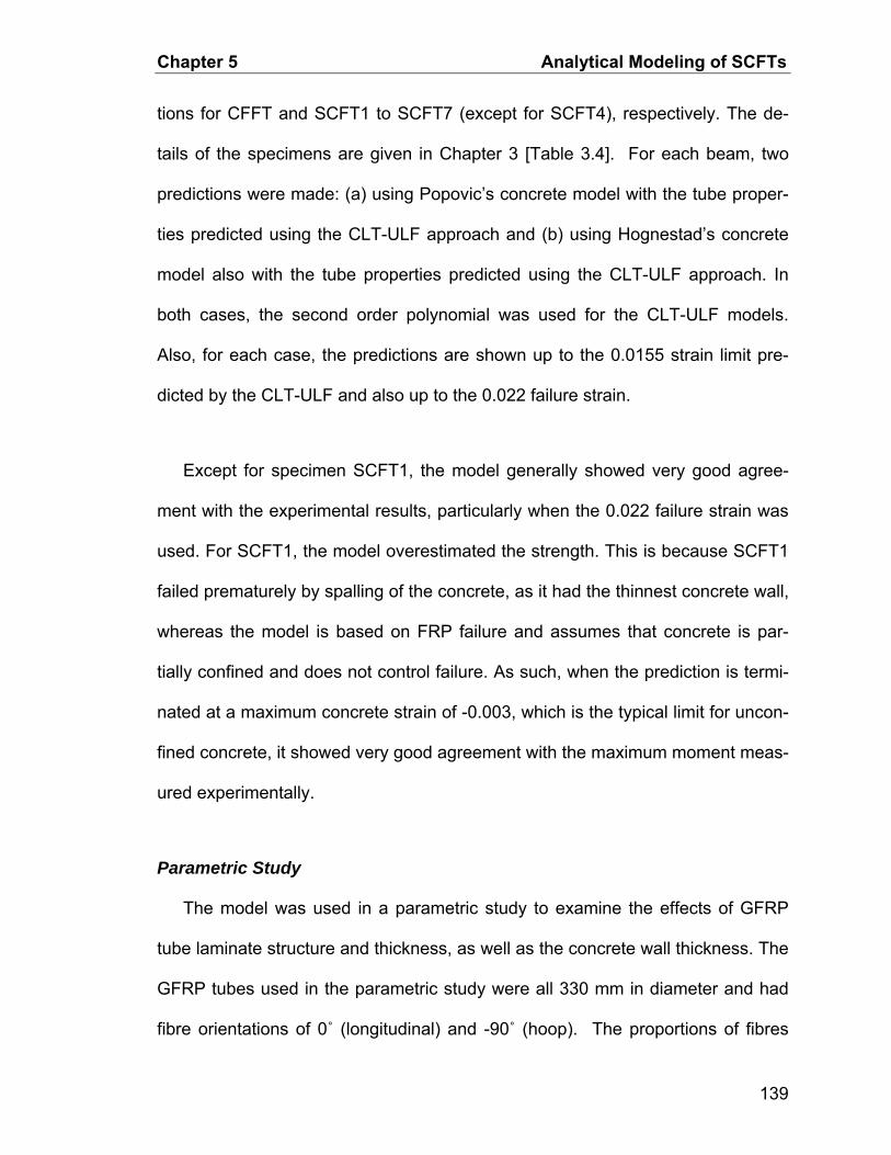
Chapter 5 Analytical Modeling of SCFTs
tions for CFFT and SCFT1 to SCFT7 (except for SCFT4), respectively. The de-
tails of the specimens are given in Chapter 3 [Table 3.4]. For each beam, two
predictions were made: (a) using Popovic’s concrete model with the tube proper-
ties predicted using the CLT-ULF approach and (b) using Hognestad’s concrete
model also with the tube properties predicted using the CLT-ULF approach. In
both cases, the second order polynomial was used for the CLT-ULF models.
Also, for each case, the predictions are shown up to the 0.0155 strain limit pre-
dicted by the CLT-ULF and also up to the 0.022 failure strain.
Except for specimen SCFT1, the model generally showed very good agree-
ment with the experimental results, particularly when the 0.022 failure strain was
used. For SCFT1, the model overestimated the strength. This is because SCFT1
failed prematurely by spalling of the concrete, as it had the thinnest concrete wall,
whereas the model is based on FRP failure and assumes that concrete is par-
tially confined and does not control failure. As such, when the prediction is termi-
nated at a maximum concrete strain of -0.003, which is the typical limit for uncon-
fined concrete, it showed very good agreement with the maximum moment meas-
ured experimentally.
Parametric Study
The model was used in a parametric study to examine the effects of GFRP
tube laminate structure and thickness, as well as the concrete wall thickness. The
GFRP tubes used in the parametric study were all 330 mm in diameter and had
fibre orientations of 0˚ (longitudinal) and -90˚ (hoop). The proportions of fibres
139

Chapter 5 Analytical Modeling of SCFTs
(longitudinal: hoop) considered were (1:9), (1:1), and (9:1), where, for example, a
(9:1) tube indicates that 90% of the fibres are oriented in the longitudinal direc-
tion. The Tubes are denoted as A, B, and C. Three tube thicknesses were con-
sidered for each laminate structure, 3 mm, 6 mm, and 9 mm so as to provide (D/t)
ratios of 110, 55, and 37, respectively. The tube laminate structures, including
thicknesses of the layers as a percentage of the total thickness, are shown in
Table 5.1. The different fibre proportions of tubes A, B, and C resulted in differ-
ent effective elastic modulii and strengths, as calculated from CLT-ULF. These
are shown in Table 5.2. Figure 5-18 shows the predicted stress-strain curves of
the three different laminate structures, the curves were fitted with a parabola and
extended to a strain of 0.022.The concrete strength cf ′ was assumed to be 60
MPa, which is a valid assumption as spun-cast concrete tends to have high
strengths as mentioned in Chapter 2. The objective of this exercise was to find
the optimum concrete wall thickness for different tube thicknesses and laminate
structures. For each case of a laminate structure and a tube thickness, the con-
crete wall thickness was increased from zero to the value of the radius (i.e. totally
filled), in increments of 0.05D. As such a total of 99 moment-curvature plots were
established and are presented in Appendix B.
Figure 5-19 to Figure 5-21 show the variation of the ultimate moment of each
case, Mu, as a ratio of the ultimate moment of the totally filled tube, Mufull, with the
concrete wall thickness represented in terms of inner-to-outer diameter ratio
(Di/Do). The figures are for tubes A, B, and C with fibre ratios (1: 9), (1: 1), and (9:
1), respectively. It should be noted that for hollow tubes (i.e. Di/Do = 1.0) Mu was
140

Chapter 5 Analytical Modeling of SCFTs
calculated using the developed model (based on strength criteria) and also using
Equation 5-39 (based on local buckling criteria), and the lower value was consid-
ered. Also, in very thin concrete walls (i.e. Di/Do = 0.7 to 0.9), the analytical model
was used but the concrete strain was limited to -0.003, rather than the extended
strain softening, because of the likelihood of spalling as occurred in specimen
SCFT1. In this case, the higher value of moment from the model or Equation 5-39
based on buckling was selected.
Effect of Tube Laminate structure
Figure 5-19, Figure 5-20, and Figure 5-21 show that at low (Di/Do) ratios (i.e.
very thick concrete walls); the (Mu/Mufull) ratio equals one. This reflects the fact
that the concrete wall thickness is larger than the neutral axis depth and as such
the extra concrete on the tension side does not affect the strength. The idea,
then, is that the ratio (Di/Do) at which the moment ratio reduces from unity is con-
sidered the optimum. By examining Figure 5-19 to Figure 5-21, we see that this
optimum (Di/Do) varies with the laminate structure. The more fibres the tube has
longitudinally (for a given thickness) the lower the optimum (Di/Do) ratio (i.e. more
concrete is needed). This is very clearly reflected in Figure 5-22, which shows
(Di/Do) optimum versus the percentage of fibres in the longitudinal direction.
Effect of FRP Tube Thickness
Figure 5-23 summarizes the findings of Figure 5-19 to Figure 5-21 by showing
the variation of optimum (Di/Do) with FRP tube thickness in different laminate
structures. It appears that for very thin to medium thickness tubes (i.e. 3 mm to 6
141

Chapter 5 Analytical Modeling of SCFTs
mm or Do/t of 55 to 110); the optimum (Di/Do) ratio reduces as the thickness in-
creases. However, for medium to large tube thicknesses (i.e. 6 mm to 9 mm or
Do/t of 37 to 55) there is no effect of the tube thickness on (Di/Do) optimum.
142
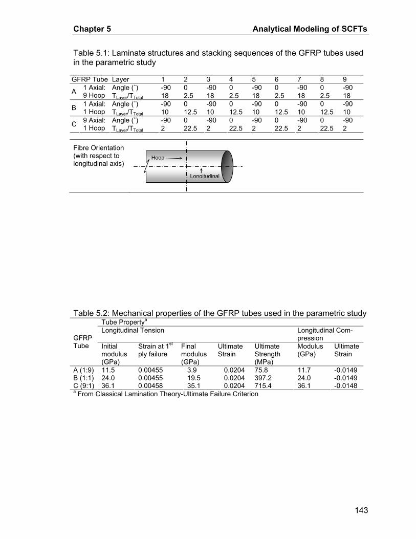
Chapter 5 Analytical Modeling of SCFTs
Table 5.1: Laminate structures and stacking sequences of the GFRP tubes used in the parametric study
GFRP Tube Layer 1 2 3 4 5 6 7 8 9 Angle (˚) -90 0 -90 0 -90 0 -90 0 -90 A 1 Axial:
9 Hoop TLayer/TTotal 18 2.5 18 2.5 18 2.5 18 2.5 18 Angle (˚) -90 0 -90 0 -90 0 -90 0 -90 B 1 Axial:
1 Hoop TLayer/TTotal 10 12.5 10 12.5 10 12.5 10 12.5 10 Angle (˚) -90 0 -90 0 -90 0 -90 0 -90 C 9 Axial:
1 Hoop TLayer/TTotal 2 22.5 2 22.5 2 22.5 2 22.5 2
Fibre Orientation (with respect to longitudinal axis)
Longitudinal
Hoop
Table 5.2: Mechanical properties of the GFRP tubes used in the parametric study Tube Propertya
Longitudinal Tension Longitudinal Com-pression GFRP
Tube Initial modulus (GPa)
Strain at 1st ply failure
Final modulus (GPa)
Ultimate Strain
Ultimate Strength (MPa)
Modulus (GPa)
Ultimate Strain
A (1:9) 11.5 0.00455 3.9 0.0204 75.8 11.7 -0.0149 B (1:1) 24.0 0.00455 19.5 0.0204 24.0 -0.0149 C (9:1) 36.1 0.00458 35.1 0.0204
397.2 715.4 36.1 -0.0148
a From Classical Lamination Theory-Ultimate Failure Criterion
143

Chapter 5 Analytical Modeling of SCFTs
Figure 5-1: Cross-section and idealized geometry of SCFTs
Concrete
R y
(c) Segment of a circle
Ro
Ri
Ric
(d) Radii of different circles
Hole
GFRP Tube General layer i
Do
i = 1 i = 2
Ac(i) Ah(i)
i = n
c h(i)
(a) Actual cross-section (b) Idealized geometry
hi
Af(i)/2
t
144

Chapter 5 Analytical Modeling of SCFTs
0
50
100
150
200
250
300
350
400
450
0 5000 10000 15000 20000 25000 30000
Strain (×10-6)
Stre
ss M
Pa erimental
Parabola0.022 strain
CLT-ULF
Exp
Figure 5-2: Predicted stress-strain behaviour of GFRP tube T1 in axial tension
0
50
100
150
200
250
300
350
400
450
0 5000 10000 15000 20000 25000
Strain (×10-6)
Stre
ss M
Pa
CLT-ULF
Experimental
Parabola0.022 strain
Figure 5-3: Predicted stress-strain behaviour of GFRP tube T2 in axial tension
145
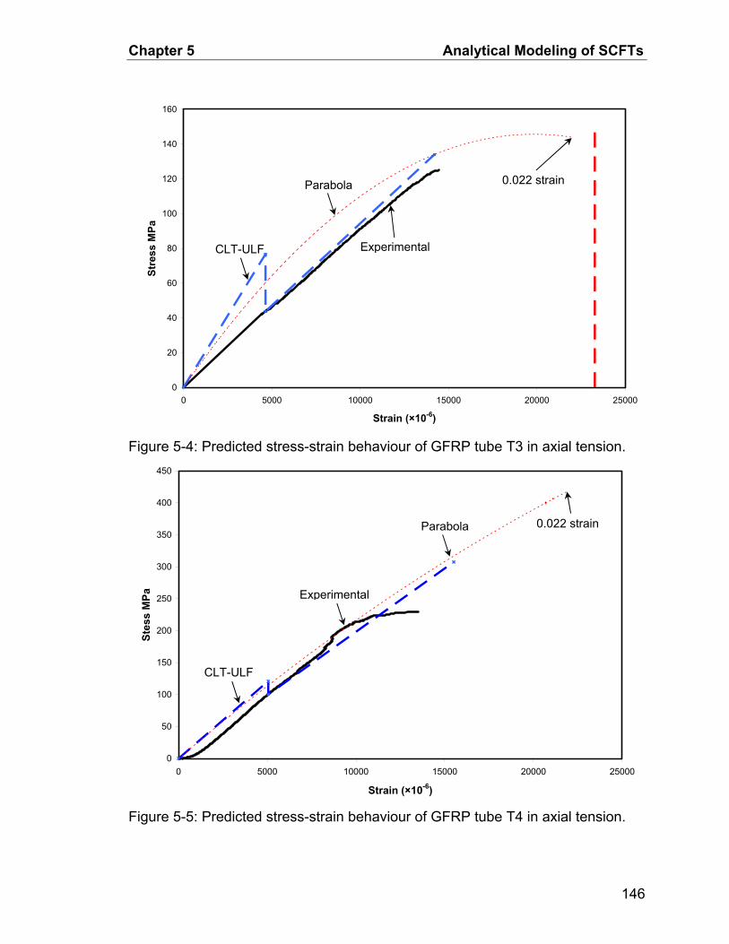
Chapter 5 Analytical Modeling of SCFTs
0
20
40
60
80
100
120
140
160
0 5000 10000 15000 20000 25000
Strain (×10-6)
Stre
ss M
Pa
CLT-ULF Experimental
Parabola 0.022 strain
Figure 5-4: Predicted stress-strain behaviour of GFRP tube T3 in axial tension.
0
50
100
150
200
250
300
350
400
450
0 5000 10000 15000 20000 25000
Strain (×10-6)
Stes
s M
Pa
CLT-ULF
Experimental
Parabola 0.022 strain
Figure 5-5: Predicted stress-strain behaviour of GFRP tube T4 in axial tension.
146
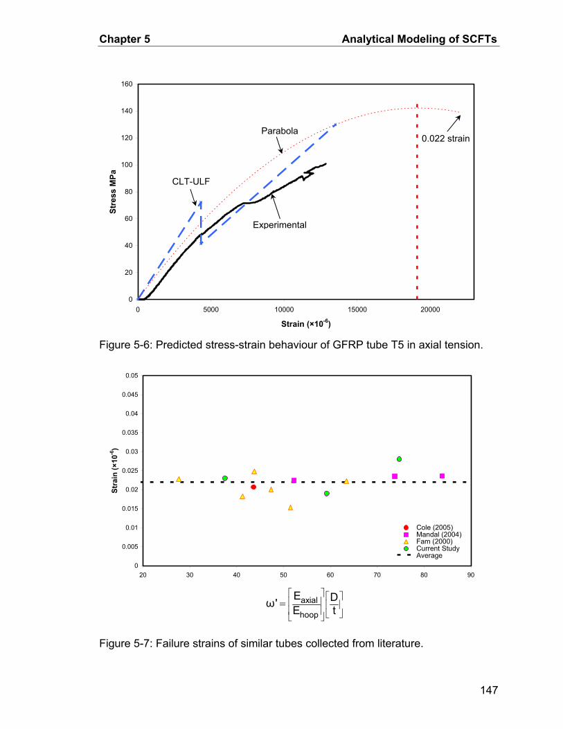
Chapter 5 Analytical Modeling of SCFTs
0
20
40
60
80
100
120
140
160
0 5000 10000 15000 20000
Strain (×10-6)
Stre
ss M
Pa CLT-ULF
Experimental
Parabola0.022 strain
Figure 5-6: Predicted stress-strain behaviour of GFRP tube T5 in axial tension.
0
0.005
0.01
0.015
0.02
0.025
0.03
0.035
0.04
0.045
0.05
20 30 40 50 60 70 80 90
Stra
in (×
10-6
)
Cole (2005)Mandal (2004)Fam (2000)Current StudyAverage
axial
hoop
E Dω ' E t⎡ ⎤ ⎡ ⎤⎢ ⎥ ⎢ ⎥⎢ ⎥ ⎣ ⎦⎣ ⎦
=
Figure 5-7: Failure strains of similar tubes collected from literature.
147

Chapter 5 Analytical Modeling of SCFTs
Compression
Strain
f′c
Stre
ss
fcr
εcε′c fc
εc εcr
Tension
(a) Popovics (1973) with extended strain softening
fc
Eco
Esec
Compression
Strain
f′c
Stre
ss
fcr
εc = 0.0038 ε′c fc
εcr
Tension
(b) Hognestad (1951) with extended strain softening
Eco
0.85 f′c
Figure 5-8: Concrete stress-strain curves used in the proposed model.
Strains
ε(i)
General layer i
D N.A.
c CC(i)
ff(i) TF(i)
CF(i)ff(i)
FRP Stresses
and Forces
TC(i)
fc(i)
Concrete Stresses
and Forces
εt
εb
ψ
h(i)
ε(i)
Idealized Cross-Section
Geometry
i = 1 i = 2
Ac(i) Af(i)/2
Ah(i) i = n
Figure 5-9: Stress and strain distributions on the cross-section of SCFTs
148
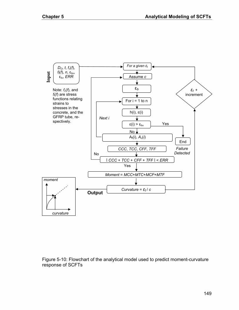
Chapter 5 Analytical Modeling of SCFTs
For a given εtDO, t, fc(f), ff(f), n, εbu, εtu, ERR
Figure 5-10: Flowchart of the analytical model used to predict moment-curvature response of SCFTs
εt + increment
Inpu
t
Assume c
εb
For i = 1 to n
h(i), ε(i)
ε(i) > εbu
End
Failure Detected
Yes
No Af(i), Ac(i)
Next i
CCC, TCC, CFF, TFF
| CCC + TCC + CFF + TFF | < ERR No
Moment = MCC+MTC+MCF+MTF
Yes
Curvature = εt / c
Note: fc(f), and ff(f) are stress functions relating strains to stresses in the concrete, and the GFRP tube, re-spectively.
moment
curvature
Output
149
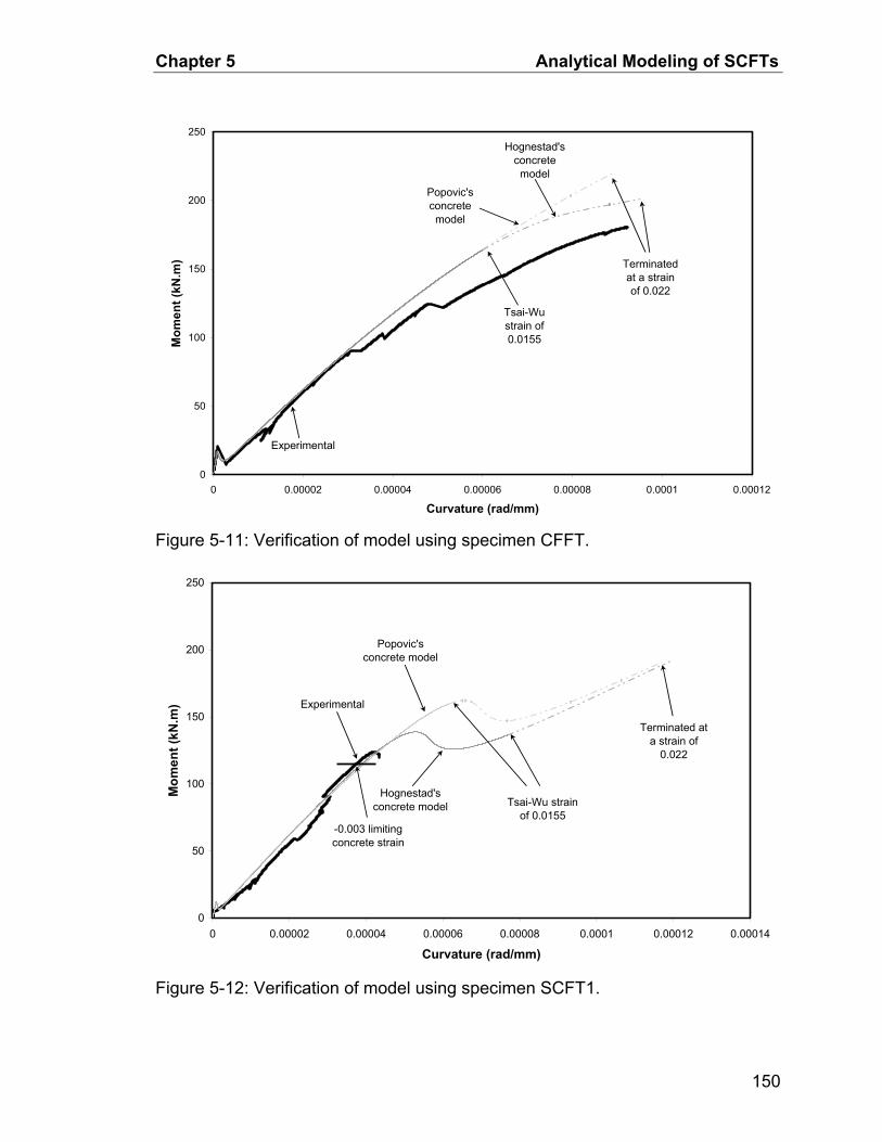
Chapter 5 Analytical Modeling of SCFTs
0
50
100
150
200
250
0 0.00002 0.00004 0.00006 0.00008 0.0001 0.00012
Curvature (rad/mm)
Mom
ent (
kN.m
)
Experimental
Popovic's concrete model
Hognestad's concrete model
Tsai-Wu strain of 0.0155
Terminated at a strain of 0.022
Figure 5-11: Verification of model using specimen CFFT.
0
50
100
150
200
250
0 0.00002 0.00004 0.00006 0.00008 0.0001 0.00012 0.00014
Curvature (rad/mm)
Mom
ent (
kN.m
) Experimental
Popovic's concrete model
Hognestad's concrete model Tsai-Wu strain
of 0.0155
Terminated at a strain of
0.022
-0.003 limiting concrete strain
Figure 5-12: Verification of model using specimen SCFT1.
150

Chapter 5 Analytical Modeling of SCFTs
0
50
100
150
200
250
0 0.00002 0.00004 0.00006 0.00008 0.0001 0.00012
Curvature (rad/mm)
Mom
ent (
kN.m
)
Experimental
Popovic's concrete model
Hognestad's concrete
model
Tsai-Wu strain of 0.0155
Terminated at a
strain of 0.022
Figure 5-13: Verification of model using specimen SCFT2.
0
50
100
150
200
250
0 0.00002 0.00004 0.00006 0.00008 0.0001 0.00012
Curvature (rad/mm)
Mom
ent (
kN.m
)
Experimental
Popovic's concrete
model
Hognestad's concrete model
Tsai-Wu strain of 0.0155
Terminated at a strain of 0.022
Figure 5-14: Verification of model using specimen SCFT3.
151
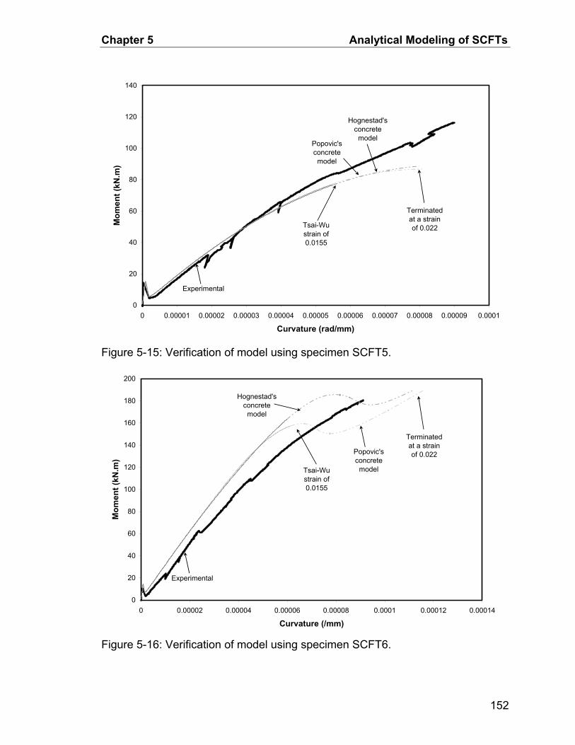
Chapter 5 Analytical Modeling of SCFTs
0
20
40
60
80
100
120
140
0 0.00001 0.00002 0.00003 0.00004 0.00005 0.00006 0.00007 0.00008 0.00009 0.0001
Curvature (rad/mm)
Mom
ent (
kN.m
)
Experimental
Popovic's concrete
model
Hognestad's concrete
model
Tsai-Wu strain of 0.0155
Terminated at a strain of 0.022
Figure 5-15: Verification of model using specimen SCFT5.
0
20
40
60
80
100
120
140
160
180
200
0 0.00002 0.00004 0.00006 0.00008 0.0001 0.00012 0.00014
Curvature (/mm)
Mom
ent (
kN.m
)
Experimental
Popovic's concrete
model
Hognestad's concrete
model
Tsai-Wu strain of 0.0155
Terminated at a strain of 0.022
Figure 5-16: Verification of model using specimen SCFT6.
152
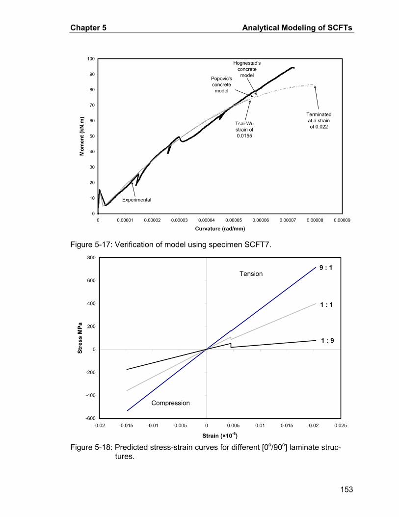
Chapter 5 Analytical Modeling of SCFTs
0
10
20
30
40
50
60
70
80
90
100
0 0.00001 0.00002 0.00003 0.00004 0.00005 0.00006 0.00007 0.00008 0.00009
Curvature (rad/mm)
Mom
ent (
kN.m
)
Experimental
Popovic's concrete model
Hognestad's concrete model
Tsai-Wu strain of 0.0155
Terminated at a strain of 0.022
Figure 5-17: Verification of model using specimen SCFT7.
-600
-400
-200
0
200
400
600
800
-0.02 -0.015 -0.01 -0.005 0 0.005 0.01 0.015 0.02 0.025
Strain (×10-6)
Stre
ss M
Pa
Compression
Tension9 : 1
1 : 1
1 : 9
Figure 5-18: Predicted stress-strain curves for different [0o/90o] laminate struc-
tures.
153
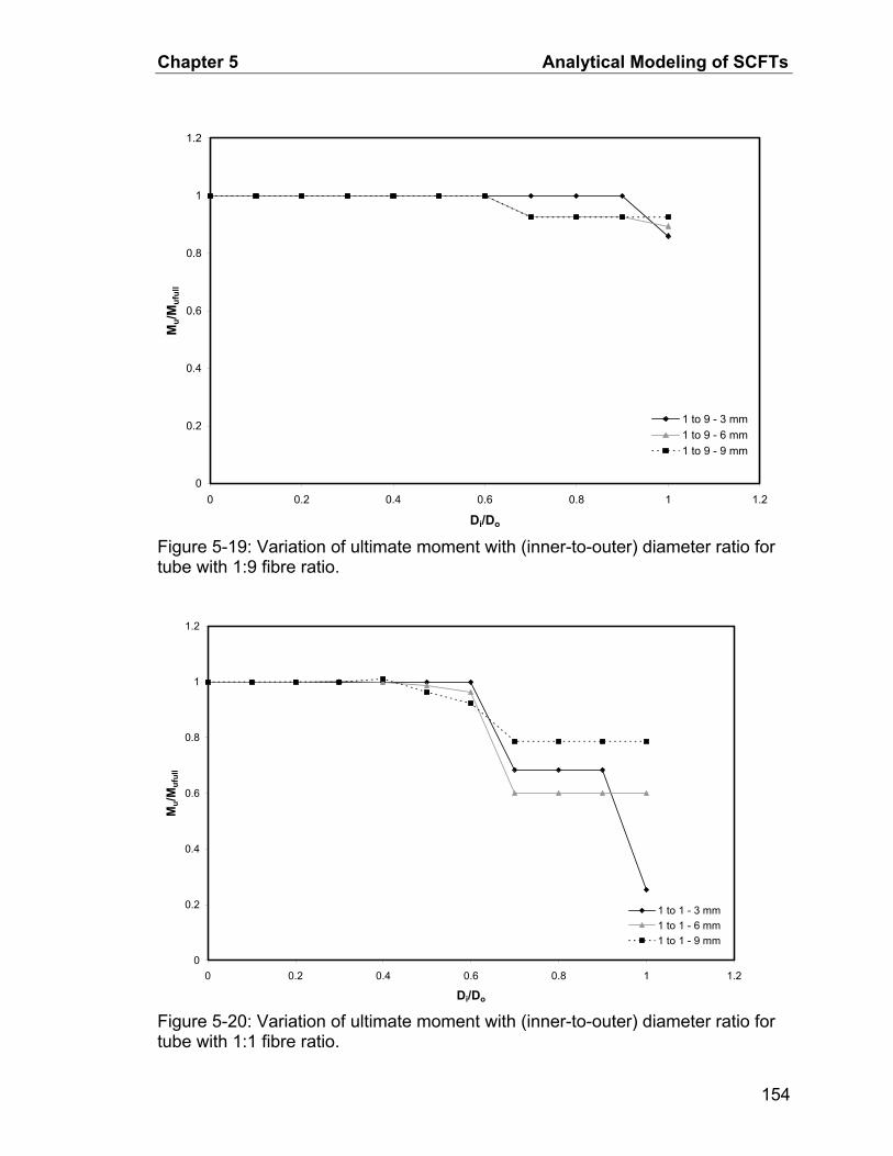
Chapter 5 Analytical Modeling of SCFTs
0
0.2
0.4
0.6
0.8
1
1.2
0 0.2 0.4 0.6 0.8 1 1.2
Di/Do
Mu/M
uful
l
1 to 9 - 3 mm1 to 9 - 6 mm1 to 9 - 9 mm
Figure 5-19: Variation of ultimate moment with (inner-to-outer) diameter ratio for tube with 1:9 fibre ratio.
0
0.2
0.4
0.6
0.8
1
1.2
0 0.2 0.4 0.6 0.8 1 1.2
Di/Do
Mu/M
uful
l
1 to 1 - 3 mm1 to 1 - 6 mm1 to 1 - 9 mm
Figure 5-20: Variation of ultimate moment with (inner-to-outer) diameter ratio for tube with 1:1 fibre ratio.
154
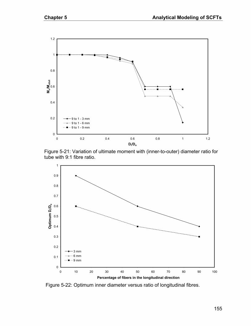
Chapter 5 Analytical Modeling of SCFTs
0
0.2
0.4
0.6
0.8
1
1.2
0 0.2 0.4 0.6 0.8 1 1.2
Di/Do
Mu/M
uful
l
9 to 1 - 3 mm9 to 1 - 6 mm9 to 1 - 9 mm
Figure 5-21: Variation of ultimate moment with (inner-to-outer) diameter ratio for tube with 9:1 fibre ratio.
0
0.1
0.2
0.3
0.4
0.5
0.6
0.7
0.8
0.9
1
0 10 20 30 40 50 60 70 80 90 100
Percentage of fibers in the longitudinal direction
Opt
imum
Di/D
o
3 mm6 mm9 mm
Figure 5-22: Optimum inner diameter versus ratio of longitudinal fibres.
155

Chapter 5 Analytical Modeling of SCFTs
0
0.1
0.2
0.3
0.4
0.5
0.6
0.7
0.8
0.9
1
0 0.005 0.01 0.015 0.02 0.025 0.03
tube t/Do
Opt
imum
Di/D
o
1 to 91 to 19 to 1
Figure 5-23: Optimum diameter of hole versus ratio of tube thickness to diameter.
156

Chapter 6 Summary and Conclusions
CHAPTER 6 : SUMMARY AND CONCLUSIONS
Summary
For the first time, a spun-cast FRP tube (SCFT) system has been fabricated.
The flexural and bond performances of SCFTs have been studied experimentally
and the flexural behaviour was also investigated analytically. Investigating the
flexural behaviour is quite relevant to the most common application this system is
intended for, namely hydro and light poles and highway overhead sign structures.
Nine full-scale specimens were tested in bending, including seven SCFT speci-
mens, one control specimen completely filled with concrete (CFFT) and another
control specimen cut from a conventional prestressed spun-cast pole with a simi-
lar diameter and length to the SCFT specimens. The effects of the concrete wall
thickness, presence of additional steel rebar, and the FRP laminate structure of
the tube, have been evaluated. As for the bond investigation, six push-off stub
specimens were cut from a SCFT specimen fabricated and tested for that pur-
pose.
An analytical model capable of predicting the moment-curvature response of
SCFTs has also been developed. This strain compatibility model, which adopts
cracked section analysis and equilibrium, uses a layer-by-layer approach, and
accounts for the material nonlinearities of the GFRP laminate and the concrete in
compression. The model was verified using the experimental results and showed
very good agreement. It was then used to conduct a parametric study to deter-
mine the critical concrete wall thickness, below which the flexural strength of the
157

Chapter 6 Summary and Conclusions
system is reduced. This was studied for different FRP tube wall thicknesses and
laminate structures.
Conclusions
Based on the experimental and analytical investigations in this study, the fol-
lowing conclusions are drawn:
1. Fabrication of spun-cast FRP tubes (SCFTs) using conventional forms and
spinning machines in existing precast facilities is feasible.
2. SCFTs have similar flexural strength to conventional prestressed spun-cast
concrete poles of a comparable reinforcement index. However, flexural stiff-
ness of SCFTs is lower than that of conventional poles, due to the lower elas-
tic modulus of GFRP relative to steel and also the absence of the prestressing
effect.
3. The tests showed that there is a maximum inner-to-outer diameter (Di/Do) ra-
tio that can be used to avoid premature inward spalling of the thin concrete
wall. For the tubes used in this experimental study this limiting (Di/Do) ratio
was 0.6, which is necessary to guarantee similar flexural strength to the totally
filled tube (CFFTs).
4. The (D /Di o) ratio has a very pronounced effect on cracking moment of SCFTs,
which is generally very low compared to the ultimate moment. However, the
effect of (D /Di o) on flexural stiffness of the tested beams, after cracking was
insignificant.
158

Chapter 6 Summary and Conclusions
5. The tube laminate structure, in terms of proportions of fibres in the longitudinal
and hoop directions, has a significant effect on the flexural strength and stiff-
ness of SCFTs. Increasing the longitudinal proportion enhances flexural
strength and stiffness significantly for a given tube thickness.
6. The parametric study showed that the optimum concrete wall thickness in
SCFTs is highly dependent on tube thickness and laminate structure. As ei-
ther the tube thickness or percentage of fibres in the longitudinal direction in-
creases, the concrete wall thickness required to produce the maximum mo-
ment also increases.
7. The addition of longitudinal steel reinforcement in SCFTs increases flexural
strength and stiffness. In this study increasing the reinforcement index from
0.5 to 0.62 has increased flexural strength and stiffness by about 45 %. How-
ever, it has no effect on ductility since steel reinforcement in this type of struc-
ture is placed in an axisymmetrical pattern. As such, most of the steel has not
yielded at failure. Steel rebar also reduced slip and allowed for higher level
concrete confinement in compression.
8. The push-off bond tests revealed a mechanical bond mechanism that is acti-
vated by small ridges protruded from the inner surface of the tube. Bond
strength seems to be maintained even at large slip and the average value is
0.15 MPa.
9. Using hydraulic grips and very short coupons is essential to obtain the full
stress-strain curves of filament-wound GFRP tubes with fibre layers at very
small angles relative to the longitudinal and hoop directions. This was con-
cluded based on a comparison between coupon tests in this study and a
159

Chapter 6 Summary and Conclusions
study by Mandal (2004) on the same tube. Premature failure of coupons oc-
curred in the current study in which mechanical grips were used.
Recommendations for Future Work
While the SCFT pole system introduced in this study clearly has merits, it is
believed that the following technical and practical aspects remain to be ad-
dressed, in order for this technology to be widely accepted at a commercial level:
1. A more effective method of delivering concrete into the FRP tube, which is
essentially a closed form, is needed. Clearly, delivering concrete manually
from one or both ends may not be practical for long poles and may lead to a
non-uniform concrete wall thickness along the pole.
2. In applications where higher stiffness is required, the use of prestressed rein-
forcement with the SCFT concept needs to be explored.
3. To maximize the advantage of the FRP tube, perhaps the conventional steel
form could be eliminated from the process (unless prestressing is required).
In this case, the possibility of spinning the FRP tube directly needs to be ex-
plored.
4. Tapered FRP tubes need to be explored as they would be more efficient and
conforming to common practice in cantilever-type poles.
5. The combined axial load and bending effects need to be studied.
6. The fatigue behaviour of the system as well as the effects of dynamic loading
and vibrations need to be studied.
160
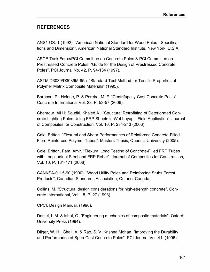
References
REFERENCES
ANS1 OS. 1 (1992). “American National Standard for Wood Poles - Specifica-tions and Dimension”, American National Standard Institute, New York, U.S.A.
ASCE Task Force/PCI Committee on Concrete Poles & PCI Committee on Prestressed Concrete Poles. “Guide for the Design of Prestressed Concrete Poles”. PCI Journal No. 42, P. 94-134 (1997).
ASTM D3039/D3039M-95a. “Standard Test Method for Tensile Properties of Polymer Matrix Composite Materials” (1995).
Barbosa, P., Helene, P. & Pereira, M. F. “Centrifugally-Cast Concrete Posts”. Concrete International Vol. 28, P. 53-57 (2006).
Chahrour, Ali H; Soudki, Khaled A.. “Structural Retrofitting of Deteriorated Con-crete Lighting Poles Using FRP Sheets in Wet Layup—Field Application”. Journal of Composites for Construction, Vol. 10, P. 234-243 (2006).
Cole, Britton. “Flexural and Shear Performances of Reinforced Concrete-Filled Fibre Reinforced Polymer Tubes”. Masters Thesis, Queen's University (2005).
Cole, Britton, Fam, Amir. “Flexural Load Testing of Concrete-Filled FRP Tubes with Longitudinal Steel and FRP Rebar”. Journal of Composites for Construction, Vol. 10, P. 161-171 (2006).
CANKSA-0 1 5-90 (1990). “Wood Utility Poles and Reinforcing Stubs Forest Products”, Canadian Standards Association, Ontario, Canada.
Collins, M. “Structural design considerations for high-strength concrete”. Con-crete International, Vol. 15, P. 27 (1993).
CPCI. Design Manual. (1996).
Daniel, I. M. & Ishai, O. “Engineering mechanics of composite materials”. Oxford University Press (1994).
Dilger, W. H., Ghali, A. & Rao, S. V. Krishna Mohan. “Improving the Durability and Performance of Spun-Cast Concrete Poles”. PCI Journal Vol. 41, (1996).
161

References
Dilger, W. H. & Rao, S. V. Krishna Mohan. “High Performance Concrete Mixtures for Spun-Cast Concrete Poles”. PCI Journal, Vol. 42, P. 82-96 (1997).
Fam, A. Z. “Concrete-Filled Fibre-Reinforced Polymer Tubes for Axial and Flex-ural Structural Members”. Ph.D. Dissertation, The University of Manitoba (2000).
Fam, A. Z. & Rizkalla, S. H. “Flexural Behavior of Concrete-Filled Fibre-Reinforced Polymer Circular Tubes”. Journal of Composites for Construction, Vol. 6, P. 123-132 (May 2002).
Fam, A. & Mandal, S. “Prestressed Concrete-Filled Fibre-Reinforced Polymer Circular Tubes Tested in Flexure”. PCI, Vol. 51, P. 42-54 (2006).
Fam, A. “Large scale testing and analysis of hybrid concrete/composite tubes for circular beam-column applications”. Construction building materials, Vol. 17, P. 507 (2003).
Fam, A. “Experimental and analytical modeling of concrete-filled fibre-reinforced polymer tubes subjected to combined bending and axial loads”. ACI structural journal, Vol. 100, P. 499 (2003).
Fam, A. “Precast piles for route 40 bridge in Virginia using concrete filled FRP tubes”. PCI journal Vol. 48, P. 32 (2003).
Fouad, F. H. & Mullinax, Edward C., Jr. “Spun Concrete Distribution Poles - An Alternative”. Transmission & Distribution, Vol. 44, P. 52-58 (April 1992).
Fouad, F. H., Scott, N. L., Calvert, E. & Donovan, M. “Performance of Spun Prestressed Concrete Poles During Hurricane Andrew”. PCI, Vol. 39, P. 102-110 (March/April 1994).
Fouad, F. H., Sherman, D. & Werner, R. J. “Spun Prestressed Concrete Poles - Past, Present, and Future”. Concrete International, Vol. 14, P. 25-29 (November 1992).
Helmi, K. “Effects of driving forces and bending fatigue on structural performance of a novel concrete-filled fibre-reinforced-polymer tube flexural pile”. Canadian Journal of Civil Engineering, Vol. 33, P. 683 (2006).
162

References
Hognestad, E. “A Study of Combined Bending and Axial Load in Reinforced Con-crete Members”. University of Illinois Engineering Experimental Station Bulletin Series No. 399, P. 128 (November 1951).
Holloman, A. “Georgia Power Performs Concrete Pole Repair”. Transmission & Distribution World, Vol. 56, P. 66K-66M (2004).
Ibrahim, S., Polyzois, D. & Hassan, S. K. “Development of Glass Fibre Rein-forced Plastics for transmission and Distribution Lines”. The Canadian Journal of Civil Engineering, Vol. 27, P. 850-858 (2000).
Kong, A. “Freeze-thaw behaviour of circular concrete members confined by fibre reinforced polymer jackets when simultaneously subjected to sustained axial loads”. Masters Thesis, Queen's University in Kingston (2005).
Popovics, S. “Numerical Approach to the Complete Stress-Strain Curve of Con-crete”. Cement and Concrete Research, Vol. 3, P. 583 (1973).
Seible. Fneder et al. "Modular advanced composite bridge system for short and medium span bridges.” Proceeding of Developments in Short and Medium Span Bridge Engineering '98. Calgary. Alberta 1998.
Sharaf, M. H., Soudki, K. A. & Van Dusen, M. “CFRP Strengthening for Punching Shear of Interior Slab–Column Connections”. Journal of Composites for Con-struction © ASCE Vol. 10, P. 410-418 (2006).
T. Yu, Y. L. Wong, J. G. Teng, S. L. Dong, E. S. Lam. “Flexural Behaviour of Hy-brid FRP-Concrete-Steel Double-Skin Tubular Members”. Journal of Composites for Construction © ASCE Vol. 10, P. 443-452 (2006).
The Institute of Electric and Electronics Engineering, Inc., New York, U.S.A. “Na-tional Electrical Safety Code” (NESC. (1997).
Thomas E. Rodgers, Jr. “Prestressed Concrete Poles: State-of-the-Art”. PCI Journal, Vol. 29, P. 52-103 (1984).
163

Appendix A
APPENDIX A : ANALYTICAL MODEL
PROGRAM LOADDEFL IMPLICIT NONE REAL, EXTERNAL :: FILLEDFORCE REAL :: EEE, STRAIN, MOMENT, CURVATURE,X,MI,DELTA REAL :: IDIA, IRAID, STRAINB, NEUTAXIS REAL :: EFRPX, EFRPY, P, ODIA, T, LT REAL, PARAMETER :: PI = 3.141592654 INTEGER ::I,N,Q,TEST2,e REAL, DIMENSION(0:200000,1:2):: MCF, LOADEFL REAL, DIMENSION(0:200000,1:2):: CURVFUL, CURVTOT LOGICAL :: TEST1, TEST, TEST3 OPEN(1,FILE='MOMCURV.CSV') OPEN(2,FILE='CONCRET.TXT') LOADEFL = 0 MCF = 0 TEST = .FALSE. TEST3= .FALSE. EFRPX = 44632.0 EFRPY = 12461.2 ODIA = 330.0 T = 5.03 IDIA = ODIA - 2*T IRAID = IDIA/2 I=1 STRAIN = 0.00001 FILLED_MC: DO CALL FALSEPOSI-TION(FILLEDFORCE,TEST1,MOMENT,CURVATURE,5.0,EEE,6.0,STRAIN,ODIA*0.5,ODIA*0.1) IF ( TEST1 == .TRUE.) THEN EXIT ENDIF MCF(I,1)= CURVATURE MCF(I,2)= MOMENT STRAINB = -(CURVATURE*ODIA - STRAIN) NEUTAXIS = - (STRAIN/STRAINB)*ODIA/(1 - STRAIN/STRAINB) WRITE (1,100) MCF(I,1), MCF(I,2), STRAIN, STRAINB, NEUTAXIS , EEE 100 format (f25.13,",",f25.13,",",f25.13,",",f25.13,",",F25.13,",",F25.13) I = I + 1 STRAIN = STRAIN + 0.00001 ENDDO FILLED_MC ENDPROGRAM LOADDEFL SUBROUTINE FALSEPOSITION(A,B,C,D,z,G,J,K,H,I)
164

Appendix A
IMPLICIT NONE REAL :: VL, VU, FL, FU, ERROR,ERRF,VROLD,VR,FR, TEST,INAU, INAL REAL ::A, C,D,F,z,G,H,I,J,K,FUNC INTEGER :: BB LOGICAL, INTENT(INOUT):: B VL= I VU= H FUNC = A(B,C,D,z,G,K,VL) FL= G FUNC =A(B,C,D,z,G,K,VU) FU=G error = 0.0001 ERRF = 1 DO WHILE ( ERRF > error) VROLD = VR IF (FL == FU) THEN VR = (VU+VL)/2 ELSE VR = VU - FU*(VL - VU)/(FL - FU) ENDIF FUNC =A(B,C,D,z,G,K,VR) FR = G IF (VR /= 0) THEN ERRF = ABS((VR -VROLD)/VR) ENDIF TEST = FL*FR IF (TEST <0) THEN VU = VR FUNC =A(B,C,D,z,G,K,VU) FU = G inau = 0 inal = inal + 1 IF (inal >= 2) THEN FL = FL /2 ENDIF ELSEIF (TEST >0) THEN VL = VR FUNC =A(B,C,D,z,G,K,VL) FL = G inal = 0 inau = inau + 1 IF (inau >= 2) THEN FU = FU/2 ENDIF ELSE ERRF = 0 ENDIF ENDDO
165
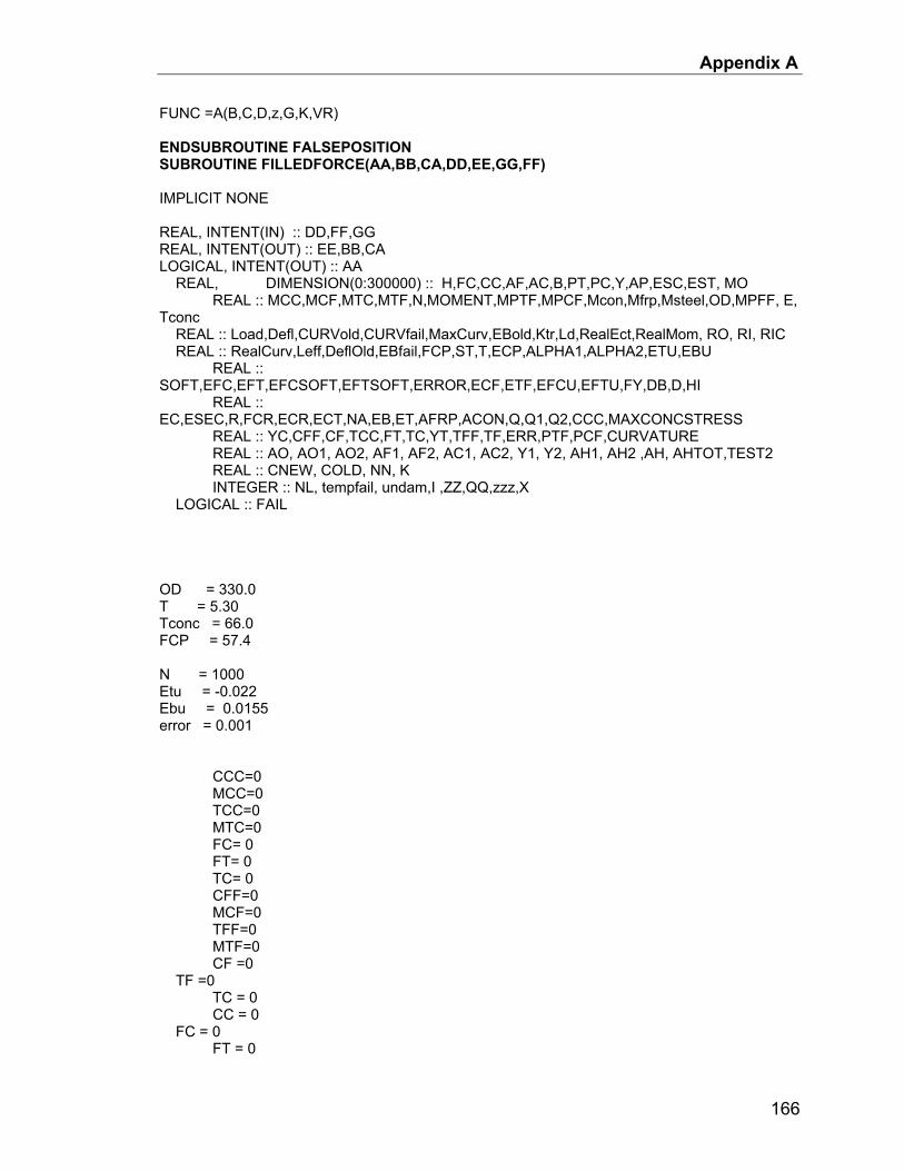
Appendix A
FUNC =A(B,C,D,z,G,K,VR) ENDSUBROUTINE FALSEPOSITION SUBROUTINE FILLEDFORCE(AA,BB,CA,DD,EE,GG,FF) IMPLICIT NONE REAL, INTENT(IN) :: DD,FF,GG REAL, INTENT(OUT) :: EE,BB,CA LOGICAL, INTENT(OUT) :: AA REAL, DIMENSION(0:300000) :: H,FC,CC,AF,AC,B,PT,PC,Y,AP,ESC,EST, MO REAL :: MCC,MCF,MTC,MTF,N,MOMENT,MPTF,MPCF,Mcon,Mfrp,Msteel,OD,MPFF, E, Tconc REAL :: Load,Defl,CURVold,CURVfail,MaxCurv,EBold,Ktr,Ld,RealEct,RealMom, RO, RI, RIC REAL :: RealCurv,Leff,DeflOld,EBfail,FCP,ST,T,ECP,ALPHA1,ALPHA2,ETU,EBU REAL :: SOFT,EFC,EFT,EFCSOFT,EFTSOFT,ERROR,ECF,ETF,EFCU,EFTU,FY,DB,D,HI REAL :: EC,ESEC,R,FCR,ECR,ECT,NA,EB,ET,AFRP,ACON,Q,Q1,Q2,CCC,MAXCONCSTRESS REAL :: YC,CFF,CF,TCC,FT,TC,YT,TFF,TF,ERR,PTF,PCF,CURVATURE REAL :: AO, AO1, AO2, AF1, AF2, AC1, AC2, Y1, Y2, AH1, AH2 ,AH, AHTOT,TEST2 REAL :: CNEW, COLD, NN, K INTEGER :: NL, tempfail, undam,I ,ZZ,QQ,zzz,X LOGICAL :: FAIL OD = 330.0 T = 5.30 Tconc = 66.0 FCP = 57.4 N = 1000 Etu = -0.022 Ebu = 0.0155 error = 0.001 CCC=0 MCC=0 TCC=0 MTC=0 FC= 0 FT= 0 TC= 0 CFF=0 MCF=0 TFF=0 MTF=0 CF =0 TF =0 TC = 0 CC = 0 FC = 0 FT = 0
166

Appendix A
hi=OD/N RO = OD/2 RI = RO - T RIC= RI - TCONC EC=4730*FCP**0.5 !EC = (3000*(FCP)**0.5+6900)*1.066 ECP = -2*FCP/EC !ECP = -0.0024 FCR=0.6*(FCP)**0.5 ECR=FCR/EC ESEC=FCP/ECP !R=ABS(EC)/(ABS(EC)-ABS(ESEC)) IF (NA >= 0) THEN TEST2 = ABS((FF -NA)/FF) ENDIF EB = GG NA=FF ET=-EB*NA/(OD-NA) AFRP=0 ACON=0 AHTOT = 0 DO I=1,(N/2) AO1 = 0 AO2 = 0 AO = 0 AC1 = 0 AC2 = 0 AH1 = 0 AH2 = 0 AH = 0 Y1 = RO - I*HI Y2 = RO - (I-1)*HI IF ((RO > Y1) .AND. (RO > Y2)) THEN AO1 = 0.5*(22/7)*RO**2 - Y1*(RO**2-Y1**2)**0.5 - ASIN(Y1/RO)*RO**2 AO2 = 0.5*(22/7)*RO**2 - Y2*(RO**2-Y2**2)**0.5 - ASIN(Y2/RO)*RO**2 END IF AO = AO1 - AO2 IF ((RI > Y1) .AND. (RI > Y2)) THEN AC1 = 0.5*(22/7)*RI**2 - Y1*(RI**2-Y1**2)**0.5 - ASIN(Y1/RI)*RI**2 AC2 = 0.5*(22/7)*RI**2 - Y2*(RI**2-Y2**2)**0.5 - ASIN(Y2/RI)*RI**2 END IF AF(I)= AO - (AC1 - AC2) AF(N-I+1) = AF(I) IF ((RIC > Y1) .AND. (RIC > Y2)) THEN
167

Appendix A
AH1 = 0.5*(22/7)*RIC**2 - Y1*(RIC**2-Y1**2)**0.5 - ASIN(Y1/RIC)*RIC**2 AH2 = 0.5*(22/7)*RIC**2 - Y2*(RIC**2-Y2**2)**0.5 - ASIN(Y2/RIC)*RIC**2 END IF AH = AH1 - AH2 AC(I)= (AC1 - AC2) - AH AC(N-I+1) = AC(I) AFRP=2*AF(I)+AFRP ACON=2*AC(I)+ACON AHTOT= AHTOT + AH ENDDO DO I = 1, N H(I)=(I-0.5)*hi E = ((EB-ET)/OD)*H(I)+ET IF (E<0)THEN !FC(I)=-1*(FCP*(E/ECP)*R)/(R-1+(E/ECP)**R) IF ( E> ECP) THEN FC(I) = -FCP*(2*E/ECP - (E/ECP)**2) ELSEIF(E<ECP) THEN FC(I) = -(FCP + ((FCP - 0.85*FCP)/(ABS(ECP) - 0.0038))*(ABS(E) - ABS(ECP))) ENDIF IF (FC(I) > 0 ) THEN FC(I) = 0 ENDIF CC(I)=FC(I)*AC(I) CCC=CCC+CC(I) MCC=MCC+CC(I)*H(I) ELSE FT=EC*E IF (E > ECR) THEN FT= 0 ENDIF TC=FT*AC(I) TCC=TCC+TC MTC=MTC+TC*H(I) ENDIF ENDDO DO I =1,N H(I)=(I-0.5)*hi E = ((EB-ET)/OD)*H(I)+ET IF (E<0) THEN !***********************************! !* ------------------------------- *! !*| FRP TUBE IN COMPRESSION |*! !* ------------------------------- *! !***********************************! !******************! !* VERIFICATION *! !******************!
168
Appendix A
!------------! ! TSAI WU ! !------------! !CF = 24954.3*E*AF(I) !T1 TSAI WU CF = 23851*E*AF(I) !T2 TSAI WU !CF = 16532*E*AF(I) !T3 TSAI WU !CF = 20461*E*AF(I) !T4 TSAI WU !CF = 16737.0*E*AF(I) !T5 TSAI WU !*******************! !* PARAMETERIC *! !*******************! !CF = 11680.7*E*AF(I) ! 1 TO 9 !CF = 23970.8*E*AF(I) ! 1 TO 1 !CF = 36085.7*E*AF(I) ! 9 TO 1 IF (E < ETU) THEN CF = 0 ENDIF IF (CF > 0 ) THEN CF = 0 ENDIF CFF=CFF+CF MCF=MCF+CF*H(I) ELSEIF (E>0) THEN !***********************************! !* ------------------------------- *! !*| FRP TUBE IN TENSION |*! !* ------------------------------- *! !***********************************! !******************! !* VERIFICATION *! !******************! !------------! ! TSAI WU ! !------------! ! TF = (23730.0*ABS(E) - 212601.0*(ABS(E)**2))*AF(I) !S1 TSAI WU TF = (22513.0*ABS(E) - 232074.0*(ABS(E)**2))*AF(I) !S4 TSAI WU !TF = (14705.0*ABS(E) - 371049.0*(ABS(E)**2))*AF(I) !S7 TSAI WU !TF = (-251065*ABS(E)**2 + 19127*ABS(E))*AF(I) !S8 TSAI WU !TF = (14846.0*ABS(E) - 387404.0*(ABS(E)**2))*AF(I) !S9 TSAI WU !TF = (-505063*ABS(E)**2 + 24243*ABS(E))*AF(I) !S1 COUPON !*********************************** !* PARAMETERIC * !*********************************** !TF = (-240561.0*E**2 + 8802.9*E)*AF(I) ! 1 TO 9 !TF = (-141270.0*E**2 + 22378.0*E)*AF(I) ! 1 TO 1 !TF = (-31196.0*E**2 + 35736.0*E)*AF(I) ! 9 TO 1
169

Appendix A
IF (E > EBU) THEN TF = 0 ENDIF IF (TF < 0 ) THEN TF = 0 ENDIF TFF=TFF+TF MTF=MTF+ TF*H(I) ENDIF ENDDO ERR= CCC+CFF+TCC+TFF MOMENT=MCC+MCF+MTC+MTF CURVATURE=ABS (ET)/NA BB = MOMENT CA = CURVATURE IF (EB> EbU) THEN IF(ABS(ERR) < 10) THEN IF(TEST2<=0.0001) THEN AA = .TRUE. ENDIF ENDIF ENDIF EE= ERR ENDSUBROUTINE FILLEDFORCE
170
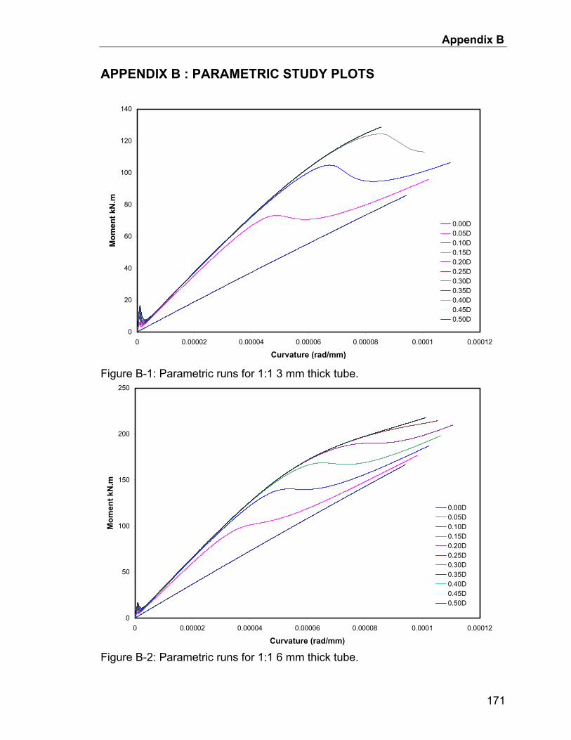
Appendix B
APPENDIX B : PARAMETRIC STUDY PLOTS
0
20
40
60
80
100
120
140
0 0.00002 0.00004 0.00006 0.00008 0.0001 0.00012
Curvature (rad/mm)
Mom
ent k
N.m
0.00D0.05D0.10D0.15D0.20D0.25D0.30D0.35D0.40D0.45D0.50D
Figure B-1: Parametric runs for 1:1 3 mm thick tube.
0
50
100
150
200
250
0 0.00002 0.00004 0.00006 0.00008 0.0001 0.00012
Curvature (rad/mm)
Mom
ent k
N.m
0.00D0.05D0.10D0.15D0.20D0.25D0.30D0.35D0.40D0.45D0.50D
Figure B-2: Parametric runs for 1:1 6 mm thick tube.
171
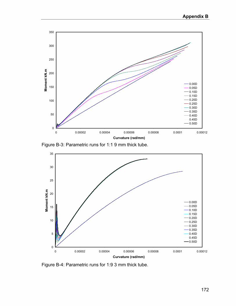
Appendix B
0
50
100
150
200
250
300
350
0 0.00002 0.00004 0.00006 0.00008 0.0001 0.00012
Curvature (rad/mm)
Mom
ent k
N.m
0.00D0.05D0.10D0.15D0.20D0.25D0.30D0.35D0.40D0.45D0.50D
Figure B-3: Parametric runs for 1:1 9 mm thick tube.
0
5
10
15
20
25
30
35
0 0.00002 0.00004 0.00006 0.00008 0.0001 0.00012
Curvature (rad/mm)
Mom
ent k
N.m
0.00D0.05D0.10D0.15D0.20D0.25D0.30D0.35D0.40D0.45D0.50D
Figure B-4: Parametric runs for 1:9 3 mm thick tube.
172

Appendix B
0
10
20
30
40
50
60
70
0 0.00002 0.00004 0.00006 0.00008 0.0001 0.00012
Curvature (rad/mm)
Mom
ent k
N.m
0.00D0.05D0.10D0.15D0.20D0.25D0.30D0.35D0.40D0.45D0.50D
Figure B-5: Parametric runs for 1:9 6 mm thick tube.
0
10
20
30
40
50
60
70
80
90
100
0 0.00002 0.00004 0.00006 0.00008 0.0001 0.00012
Curvature (rad/mm)
Mom
ent k
N.m
0.00D0.05D0.10D0.15D0.20D0.25D0.30D0.35D0.40D0.45D0.50D
Figure B-6: Parametric runs for 1:9 9 mm thick tube.
173

Appendix B
0
50
100
150
200
250
0 0.00002 0.00004 0.00006 0.00008 0.0001 0.00012
Curvature (rad/mm)
Mom
ent k
N.m
0.00D0.05D0.10D0.15D0.20D0.25D0.30D0.35D0.40D0.45D0.50D
Figure B-7: Parametric runs for 9:1 3 mm thick tube.
0
50
100
150
200
250
300
350
400
0 0.00002 0.00004 0.00006 0.00008 0.0001 0.00012
Curvature (rad/mm)
Mom
ent k
N.m
0.00D0.05D0.10D0.15D0.20D0.25D0.30D0.35D0.40D0.45D0.50D
Figure B-8: Parametric runs for 9:1 6 mm thick tube.
174

Appendix B
0
50
100
150
200
250
300
350
400
450
500
0 0.00002 0.00004 0.00006 0.00008 0.0001 0.00012
Curvature (rad/mm)
Mom
ent k
N.m
0.00D0.05D0.10D0.15D0.20D0.25D0.30D0.35D0.40D0.45D0.50D
Figure B-9: Parametric runs for 9:1 9 mm thick tube.
175