Flame Fundamentals: Theory and Modeling, Part IHong G. Im

Computational Reacting Flows Laboratory (CRFL)

Clean Combustion Research Center, KAUST

Clean Combustion Summer School

The Combustion Institute

April 1-5, 2018

Computational Reacting Flows Laboratory (CRFL)

Personnel (10 countries)

Prabhu Selvaraj

Francisco Hernandez Perez

Research Scientist

Balaji Mohan

Postdoc

Memdouh Belhi

Postdoc

Ph.D./M.S. Students

Mohammed Jaasim Wonsik Song Yu Jeong Kim Rahul Dhopeshwar

Aliou Sow

Postdoc

Stathis Tingas

Postdoc

Zhen Lu

Postdoc

Sangeeth Sanal

Minh Bau Luong

Postdoc

Erica Quadarella

Juan Restrepo Cano

KAUST: William Roberts, Robert Dibble, Bengt Johansson, Mani Sarathy, Aamir Farooq,

Min Suk Cha, Gaetano Magnotti, Deanna Lacoste, Thibault Guiberti

U. Rome: Mauro Valorani, Pietro Ciottoli, Pascuale Lapenna, Riccardo Malpica Galassi

NTU Athens: Dimitrious Goussis

Oak Ridge National Laboratory: Ramanan Sankaran

University of Michigan: Venkat Raman

University of Wisconsin: Chris Rutland, Hongjiang Li

GIST, Korea: Bok Jik Lee

Saudi Aramco: Jihad Badra, Jaeheon Sim

Contributors

Sponsored by

The Combustion Institute

Clean Combustion Research Center

KAUST Baseline

KAUST Competitive Center Funding

Saudi Aramco

• Basic scaling theory: Damköhler and Zeldovich numbers

• Revisit S-curve dynamics: steady vs. unsteady description of combustion

dynamics

• Large activation energy asymptotics

• Intrinsic flame instabilities

• Numerical modeling of thermochemistry

• Laminar flame modeling – canonical flames

• Turbulent combustion regimes

• DNS with HPC & diagnostics

• LES vs. RANS

• Turbulent combustion closure

• Application examples at KAUST – LES and RANS

Outline

Towards Efficient and Clean Combustion

• High pressure

• Lean burn

• Preheated (MILD)

• Mixed-mode

• Fuel flexible

• CO2

Highly complex!!

GE 9HA gas turbine Mazda Skyactive X

Echogen

Turbulent Nonpremixed Syngas Flames at High Pressures

The field-of-view is 20 x 20 mm and the

spatial resolution is better than 150 μm.

Non-intrusive diagnostic tools

unravel spatially and temporally

resolved information about

temperature and reactive species.

But there are challenges:

- Resolution limits

- Quantitative measurements

- Multi-dimensional imaging

Cross-validation and complimentary

collaboration with high fidelity

simulations are essential.

BASIC ASYMPTOTIC THEORY

Scaling is everything!

Damköhler Number:

Key Nondimensional Parameters in Combustion

Da =$

%=Characteristic Reaction Rate

Characteristic Flow Rate~1

6

Ze =89

:;<= Nondimensional Activation Energy

Zeldovich Number:

For typical combustion systems, Da and Ze are large.

- Turbulence may reduce Da, but not Ze

- For actual systems, there exist a number of chemical time scales,

making a definite characterization difficult.

Effects of Da and Ze: Laminar Nonpremixed Flames

Zeldovich Number:

Effect of Da

Da → ∞

Da → ∞

Da = Daq

T/Tmax

10

w/wmax

1

Ze

increase

Flame sheet limit

(Burke-Schumann

limit)

Effect of Ze

For nonpremixed flames, Ze → ∞ is a

valid asymptotic limit. Physical flame thickness ~

!

∇#~

!

%

Effects of Da and Ze: Laminar Premixed Flames

Not so simple; e.g. for equi-diffusive flames (Le = 1),

Effect of Da Effect of Ze

For premixed flames, Ze → ∞ is NOT a valid asymptotic limit.

¥T

¥-T

TTae/-

Rd

Td

x

!"#$# = exp −

*+

*,exp(−Ze

/

0#)

Ze =*+ *, − *",

*,2

~0#

04

Law, C. K., Combustion Physics (2006).

Effects of strain rates are not directly

translated to the flame thickness.

From Law (2006)

The S-Curve Behavior:

Characteristic of Reaction Nonlinearity with Large Activation Energy

• Ignition: as Da is increased from the

frozen limit, the mixture becomes

increasingly reactive, and reaches a

point at which loss cannot balance

generation.

• Extinction: as Da is decreased from the

equilibrium limit, the flame becomes

weaker, and reaches a point at which

the reaction cannot be sustained.

• Note that the S-curve shows the

STEADY response, and does not tell us

about how long it takes to ignite or

extinguish.

Equilibrium →

← Frozen

The S-Curve: Steady Combustion Response

Ze > 10

Ze < 1

Daq Daig

Da

Unsteady dynamics overlaid on the steady S-curve

Ignitable

Steady/Unsteady Combustion Characteristics

Tmax

Extinguishable

Daq Daig Da

!ig

!q

!ig / !q

One of the most commonly adopted configuration

to study laminar nonpremixed flames.

• 1-D similarity solution for simple mathematical

analysis (potential flow or opposed-jet flow)

• Easy experimental set-up (opposed-jet only)

• Parametric study on the aerodynamic effects

on flames by allowing an independent control

of the flow time scale (strain rate).

Counterflow Nonpremixed Flames

Diffusion Flame

Fuel

Oxidizer

L r (or x), u

y, v

u∂ !T∂ !r

+w∂ !T∂ !z

= DF

∂2 !T∂ !z2

+1

!r

∂∂ !r!r∂ !T∂ !r

⎛⎝⎜

⎞⎠⎟

⎡

⎣⎢

⎤

⎦⎥ +

Q

cpwF

Axisymmetric Geometry (r, z)

ur=a

2r, u

z= −az

Fendell, F.E., J. Fluid Mech. 21: 281-303 (1965)

satisfies the continuity equation.

Energy & Species Equationsλρcp

= DF = DO

⎛

⎝⎜

⎞

⎠⎟

u∂Y

F

∂ !r+w

∂YF

∂ !z= D

F

∂2YF

∂ !z2+1

!r

∂∂ !r!r∂Y

F

∂ !r⎛⎝⎜

⎞⎠⎟

⎡

⎣⎢

⎤

⎦⎥ +wF

u∂Y

O

∂ !r+w

∂YO

∂ !z= D

F

∂2YO

∂ !z2+1

!r

∂∂ !r!r∂Y

O

∂ !r⎛⎝⎜

⎞⎠⎟

⎡

⎣⎢

⎤

⎦⎥ +νwF

F[ ]+ vO O[ ]→ P[ ]

wF= ZY

OYFexp −E / R !T( )

ν =νOW

O

WF

!T−∞

YF−∞

!T∞

YO∞

1D Potential Flow Formulation

T =cP!T

QYF−∞, yF =

YF

YF−∞, yO =

YO

νYF−∞

Nondimensional Variables

r = a /D

F( )1/2!r, z = 2a /D

F( )1/2!z

Similarity approximation (Fendell, 1965)

T = T z( ), yi = yi z( ) i = F,O( )

Mathematical Reduction

x =1

2erfc

z

2

⎛⎝⎜

⎞⎠⎟=1

πe− y2dy

z/ 2

∞

∫

Coordinate transformation

so that x = 0, z→∞; x = 1, z→−∞

d2T

dx2= −2π exp z

2( )DyOyF exp −Ta /T( )

d2

dx2T + yF( ) = 0

d2

dx2T + yO( ) = 0

x = 1:

T = T∞ − β, yF = 1, yO = 0

x = 0 :

T = T∞ , yF = 0, yO =α

α =YO∞

νYF−∞, β = T∞ −T−∞

Boundary conditions:Transformed Governing Equations

Coupling Function Solutions

d2

dx2T + yF( ) = 0

d2

dx2T + yO( ) = 0

x = 1:

T = T∞ − β, yF = 1, yO = 0

x = 0 :

T = T∞ , yF = 0, yO =α

α =YO∞

νYF−∞, β = T∞ −T−∞

Boundary conditions:

yF = x +T f −T

yO =α 1− x( )+T f −T

T f = T∞ − βx

x =1

2erfc

z

2

⎛⎝⎜

⎞⎠⎟

(frozen solution)

The problem boils down to:

d 2T

dx2= −2π exp z2( )Dy

O(T )y

F(T )exp −T

a/ T( )

x = 0 :T = T∞; x = 1:T = T∞ − β,

Mathematical Reduction

Base solutions:

d2T

dx2= 0 ⇒ T f = T∞ − βx

Frozen flow:

d2T

dx2= −2π exp z

2( )DyOyF exp −Ta /T( )

x = 0 :T = T∞; x = 1:T = T∞ − β,

Equilibrium flow:

T = x +T∞ − βx0 < x < xe

(Oxidizer side):

T =α 1− x( )+T∞ − βxxe< x <1(Fuel side):

Base Solutions

α =Y

O∞

νYF−∞

, β = T∞−T

−∞

D.F.: Diffusion Flame, P.F.: Premixed Flame, F.F.: Frozen Flow, P.B.: Partial Burning

Liñán’s Regimes

Generalized theory allows the analysis of premixed flames (in the P.F. regime)

Extinction Analysis in Near-Equilibrium Regime

d2β1dξ 2

= β1 − ξ( ) β1 + ξ( )exp −δ 0−1/3 β1 + γξ( ){ }

The inner reactive-diffusive zone equation:

with boundary conditions:

dβ1

dξ= 1, ξ →∞;

dβ1

dξ= −1, ξ →−∞

δ0E

= e 1− γ( )− 1− γ( )2{

+0.26 1− γ( )3

+ 0.055 1− γ( )4}

Reduced Damköhler number at extinction:

For small values of 1− γ( )

For hot boundary ignition: β = T

∞−T

−∞= O 1( )

Ignition Analysis in Nearly Frozen Regime

The inner structure equation:

with the reduced Damköhler number:

Δ = β −1

zε

−2αDexp −Ta

/ T∞( )

χ 2 d2θ

1

dχ 2= −Δ χ − βθ

1( )exp θ1− χ( )

θ1

0( ) = 0,dθ

1

dχ∞( ) = 0

Correlations for the ignition criterion:

D

Iα exp −T

a/ T

∞( ) zε

−2! 2e

−2 1− β( )−2

2β − β 2( )

zε2= − ln 8πε 2

zε2

/ β 21− β( )

2⎡⎣⎢

⎤⎦⎥

β = O 1( )

Go/No-go Criterion

(Ignition turning point)

Monotonic as !" > !$%

Adiabatic system with a homogeneous reactant mixture.

Nondimensionalization:

ρ

0c

v

dT

dt= −Q

c

dcF

dt= BQ

cc

Fexp −T

a/ T( )

!T =c

vρ

0T

Qcc

F ,0

=c

vT

qcY

F ,0

; !cF=

cF

cF ,0

T = T

0, c

F= c

F ,0; t = 0I.C.:

Coupling function:

d

dt

!T + !cF( ) = 0; !T − !T

0= 1− !c

F

d !T

dt= B 1+ !T

0− !T( )exp − !T

a/ !T( ) I.C.:

!T = !T

0; t = 0

Unsteady Ignition Analysis

Asymptotic expansion:

!T = !T0+ εθ t( )+O ε

2( ) ε = !T

0

2/ !T

0

!c

F= 1 + !T

0− !T = 1− εθ t( ) " 1+O ε( )

The solution:

I.C.: θ τ = 0( ) = 0

dθ

dτ= exp θ( )

tig= t

c=ε

Bexp

!Ta

!T0

⎡

⎣⎢

⎤

⎦⎥

tig=

cv!T0

2 / !Ta( )

qcY

F ,0Bexp − !T

a/ !T

0( )

θ τ( ) = − ln 1−τ( )

Ignition at τ = 1

or

Law, Combustion Physics (2016)

Unsteady Ignition Analysis

• Practical Relevance to Turbulent Combustion

- Self-turbulization + Baroclinic Torque

⇒ Enhanced burning (turbulence-flame interaction)

• Primary Modes of Intrinsic Flame Instabilities

– Hydrodynamic (Darrieus 1938, Landau 1944)

• Streamline deformation due to thermal expansion

– Diffusive-Thermal (Turing 1952, Sivashinsky1977)

• Thermal vs. mass diffusion imbalance

– Buoyancy-Induced (Rayleigh 1883, Taylor 1950)

• Gravitational acceleration of product gases

– Viscosity-Induced (Saffman and Taylor 1958)

• Combustion in a narrow channel

Intrinsic Flame Instabilities

Rich propane-air

cellular flame in

state of chaotic self-

motion (Sabathier

et al., 1981)

(Strehlow, 1968)

Lean butane-air

(stable)

Lean hydrogen-air

(unstable)

• Basic Assumptions

– Constant flame speed, normal to the front

– Flame is a discontinuous surface

δ =

D/ L→ 0

F(x,t) = x − f y, z,t( ) = 0

Unburned Burned

ρ = 1

T = 1

Y = 1

ρ = 1/ 1+ q( )

T = 1+ q

Y = 0

n =∇F

∇F

δ → 0

Darrieus-Landau Model (1945)

′v = exp ωt + ik1y + ik2z( )v

′p = exp ωt + ik1y + ik2z( ) p

f = exp ωt + ik1y + ik2z( )A

ω = ℑ k( )

Method of normal modes

& Seek dispersion relation

Streamline deflection due to heat release

Unconditionally unstable!

!

k

Higher heat release

! ~ k

Su Sbu > Su u > Sb

u < Su u < Sb

Su

Sb

2 + q( )ω 2+ 2 1+ q( )kω + qk g − 1+ q( )k⎡⎣ ⎤⎦ = 0Dispersion relation:

D-L Instability: Physical Mechanism

Paradox can be resolved by allowing variable SL

SL = 1− µ∇2f = 1− µ / R Markstein (1950)

• Asymptotic Structure of a Premixed Flame

Diffusive-Thermal Model: Sivashinsky (1979)

O δ / β( )

O δ( ) O 1( ) Fluid dynamic

scaleFlame zone

Reaction zone

Unburned

gases

Burned

gases

D

L= O δ( )

R

D

= O1

β⎛⎝⎜

⎞⎠⎟= O ε( )

Large Activation Energy Asymptotics

D-T Instability: Physical Mechanism

Dispersion Relation 64ω3+ 192k

2+ 32 + 8l − l

2( )ω 2

+2 2 + 8k2+ l( ) 1+12k2( )ω + 2 + 8k

2+ l( )

2

k2= 0

l = Le −1( ) / ε

Aerodynamics of Flame: The Flame Stretch

Examples of stretched flames

Law, C. K., Combustion Physics (2006).

Markstein (1950)

Asymptotic Analysis for Low Stretch Flames

Clavin & Williams (1982), Clavin & Garcia (1983)

SL

SL,κ =0

= 1− µ∇f (heuristic curvature effect)

SL

SL,κ =0

= 1− Lκ + = 1− MaKa

Ma =L

δ Markstein number; Ka =

δκ

SL

Karlovitz number

Ma =1

γJ +

β Le −1( )2

1− γγ

⎛⎝⎜

⎞⎠⎟

D

γ =T

b−T

u

Tb

; J =λ

λ Tu

( )dT

TTu

Tb

∫

D =T

u

Tb−T

u

⎛

⎝⎜⎞

⎠⎟λ

λ Tu

( )ln

Tb−T

u

T −Tu

⎛

⎝⎜⎞

⎠⎟dT

TTu

Tb

∫

The Markstein Number

Diffusive-Thermal Instability

• Self-turbulization ⇒ turbulent kinetic energy backscatter

Darrieus-Landau Instability

• Increases with the system size

• Likely a significant (dominant?) factor in ST enhancement

- Creta et al. (2016)

- The “Lambda” Flame, Aspden (2016)

Intrinsic Flame Instabilities – How Does It Matter?

Towery, Poludnenko, et al., Phys. Fluids (2016)

Creta et al., Phys. Review E (2016)

Unsteady Effects (Im & Chen, 2000)- Flame response to harmonic oscillation in strain rate

M =S

L,max− S

L,min

Kamax

− Kamin

= F ω( ) Markstein transfer function

a = a

01+ Asinωt( )

Ma in Unsteady Flames – Transfer Function

NUMERICAL MODELING OF

THERMOCHEMISTRY

Building blocks for detailed flame simulations

Convective (Nonconservative) Form

Dρ

Dt+ ρ∇⋅v = 0

ρDv

Dt= −∇⋅P+ ρ Y

ifi∑

ρDe

Dt= −∇⋅q− P :∇v + ρ Y

ifi⋅V

i∑

ρDY

i

Dt= −∇⋅ ρV

iYi( )+wi

, i = 1,!,N

Conservation Equations for Multicomponent Reacting Flows

∂ρ

∂t= −∇⋅(ρu)

∂ρv

∂t= −∇⋅(P+ ρvv)+ ρ Y

ifi∑

∂

∂tρE( ) = −∇⋅ ρvE + v ⋅P+ q[ ]+ ρ v +V

i( ) ⋅Yifi∑

∂ρYi

∂t= −∇⋅ ρvY

i( )−∇⋅ ρViYi( )+wi

, i = 1,!,N

E = e+1

2v ⋅v

⎛⎝⎜

⎞⎠⎟

Conservative Form

Stress Tensor:

P = [ p + (

2

3µ −κ )∇⋅v]U − µ (∇v)+ (∇v)T⎡⎣ ⎤⎦

Bulk viscosity = 0 (Stokes assumption)

Unit tensor

Constitutive Relations – Nonreacting Flows

Heat Flux Vector: q = −λ∇T + ρ hiYiVii=1

N

∑ +X jDi

T

WiDij

⎛

⎝⎜⎞

⎠⎟Vi −Vj( )+ qrad

j=1

N

∑i=1

N

∑Fourier

conductionenthalpy transport

by diffusion Dufour effectradiation

p = p(e,ρ)Equation of State: p = ρR0T /W = ρR0T Yi/W

i( )i=1

N

∑for ideal gas:

Enthalpy & Internal Energy: h = Y

ih

i∑ = e+ p / ρ

hi= h

f ,i

0 T 0( )+ cp,iT

0

T

∫ dT , cp,i

(T ) = am,i

T m

m=0

6

∑ NASA polynomial( )

Conversion: Xi=

Yi/W

i

Yj/W

j( )j=1

N

∑; Y

i=

XiW

i

XjW

j( )j=1

N

∑ X

i−Y

i

Reaction Rate for Species i:

′νi,k

Mi

i=1

N

∑ ↔ ′′νi,k

Mi

i=1

N

∑ k = 1,!, K

wi=W

iω̂

i=W

i′′νi,k− ′ν

i,k( )k=1

K

∑ kf ,k

Xjp

R0T

⎛

⎝⎜

⎞

⎠⎟

′ν j ,k

j=1

N

∏ − kb,k

Xjp

R0T

⎛

⎝⎜

⎞

⎠⎟

′′νj ,k

j=1

N

∏⎡

⎣

⎢⎢

⎤

⎦

⎥⎥

For a system of K reversible reactions:

kf ,k

= AkT

βk exp −

Ek

RT

⎛

⎝⎜⎞

⎠⎟, k

b,k=

kf ,k

KC ,k

Constitutive Relations – Reaction Source Terms

Note:

• For a given species, the number of exponential function evaluations ~ K

• Inside the reaction routine, there are numerous operations to convert mole to

mass fractions.

A

k E

k β

k

N

K

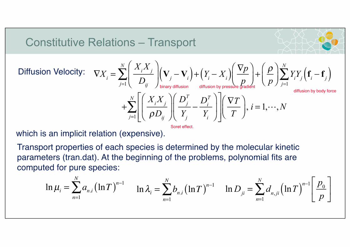
Constitutive Relations – Transport

Diffusion Velocity:

∇Xi=

XiX

j

Dij

⎛

⎝⎜

⎞

⎠⎟ V

j− V

i( )j=1

N

∑ + Yi− X

i( )∇p

p

⎛⎝⎜

⎞⎠⎟+

ρp

⎛⎝⎜

⎞⎠⎟

YiY

jf

i− f

j( )j=1

N

∑

+X

iX

j

ρDij

⎛

⎝⎜

⎞

⎠⎟

Dj

T

Yj

−D

i

T

Yi

⎛

⎝⎜

⎞

⎠⎟

⎡

⎣⎢⎢

⎤

⎦⎥⎥

∇T

T

⎛⎝⎜

⎞⎠⎟

, i = 1,!, Nj=1

N

∑

binary diffusion diffusion by pressure gradientdiffusion by body force

Soret effect.

Transport properties of each species is determined by the molecular kinetic

parameters (tran.dat). At the beginning of the problems, polynomial fits are

computed for pure species:

lnµi= a

n,ilnT( )

n−1

n=1

N

∑ lnλi= b

n,ilnT( )

n−1

n=1

N

∑

ln Dji= d

n, jilnT( )

n−1

n=1

N

∑p

0

p

⎡

⎣⎢

⎤

⎦⎥

which is an implicit relation (expensive).

L00,00

L00,10

0

L10,00

L10,10

L10,01

0 L01,10

L01,01

⎛

⎝

⎜⎜⎜

⎞

⎠

⎟⎟⎟

a00

1

a10

1

a01

1

⎛

⎝

⎜⎜⎜⎜

⎞

⎠

⎟⎟⎟⎟

=

0

X

X

⎛

⎝

⎜⎜

⎞

⎠

⎟⎟

λ = λtr+ λ

int

With the solutions for

The L Matrix: block submatrices

mole fraction vector

a00

1, a

10

1, a

01

1

λtr= − X

jaj ,10

1

j=1

N

∑ , λint= − X

jaj ,01

1

j=1

N

∑ Di

T=8m

iXi

5R0ai,00

1

Multicomponent Properties (EGLib)

D̂ij= X

i

16T

25p

W

Wj

Pij− P

ii( ), P = L00,00( )

−1

Vi= −

1

XiW

WjD̂ijdj−

j≠1

N

∑Di

T

ρYi

∇T

Tmulticomponent diffusion coeff.

where

Soret

Ern & Giovangigli, http://www.cmap.polytechnique.fr/www.eglib/

Computational cost ~ N2

Transport properties are approximated as a weighted average:

µ =Xiµi

XjΦ

ijj=1

N

∑i=1

N

∑ Φij=1

81+

Wi

Wj

⎛

⎝⎜

⎞

⎠⎟

−1/2

1+µi

µj

⎛

⎝⎜

⎞

⎠⎟

1/2

Wj

Wi

⎛⎝⎜

⎞⎠⎟

1/4⎛

⎝⎜⎜

⎞

⎠⎟⎟

2

(Wilke, 1950)

λ =1

2Xiλi

i=1

N

∑ +1

Xi/ λ

ii=1

N∑⎛

⎝⎜⎜

⎞

⎠⎟⎟

(Mathur, 1967)

Mixture-Averaged Formula

Vi= −

1

Xi

D̂imdi−Di

T

ρYi

∇T

T

di= ∇X

i+ X

i− X

j( )∇p

pD̂im=

1−Yi

Xj/D

jij≠1

N

∑where

mixture-averaged diffusion coeff.

MODELING OF CANONICAL LAMINAR FLAMES

Homogeneous reactor

Continuous stirred tank reactor (CSTR)

Premixed flames

Opposed-jet nonpremixed flames

Constant Volume:

Homogeneous Reactor

cv

dT

dt= −

1

ρe

iW

iω̂

i

i=1

N

∑ ,dY

i

dt=

Wi

ρω̂

i

Constant Pressure:

cp

dT

dt= −

1

ρh

iW

iω̂

ii=1

N

∑ ,dY

i

dt=

Wi

ρω̂

i

0D IC Engine:

cv

dT

dt= −

1

ρe

iW

iω̂

ii=1

N

∑ +p

m

dV (t)

dt

dYi

dt=

Wi

ρω̂

i

Associated Numerics:

• Stiff time integrator

• One-step Runge-Kutta

• Multistep (backward

differentiation – CVODE)

residence time

Continuous Stirred Tank Reactor

τ

cstr=V

cstr/ Q

dYi

dt=

Wi

ρω̂

i+

Yi,in

−Yi( )

τcstr

cp

dT

dt= −

1

ρh

iW

iω̂

i+

hin− h( )

τcstri=1

N

∑

Extended to zone models- Reactor volume broken into M well-mixed zones

dYi

(m)

dt=

Wi

ρω̂

i+ f

kmY

i

(k ) − fmk

Yi

(m)( ),k=0

M+1

∑ k = 1,…, M

Associated Numerics:

• Stiff time integrator

• One-step Runge-Kutta

• Multistep (backward

differentiation – CVODE)

0

1 2

3 4

5

12f

21f

01f

45f- Commonly used as turbulent combustion closure

(PaSR: partially stirred reactor model)

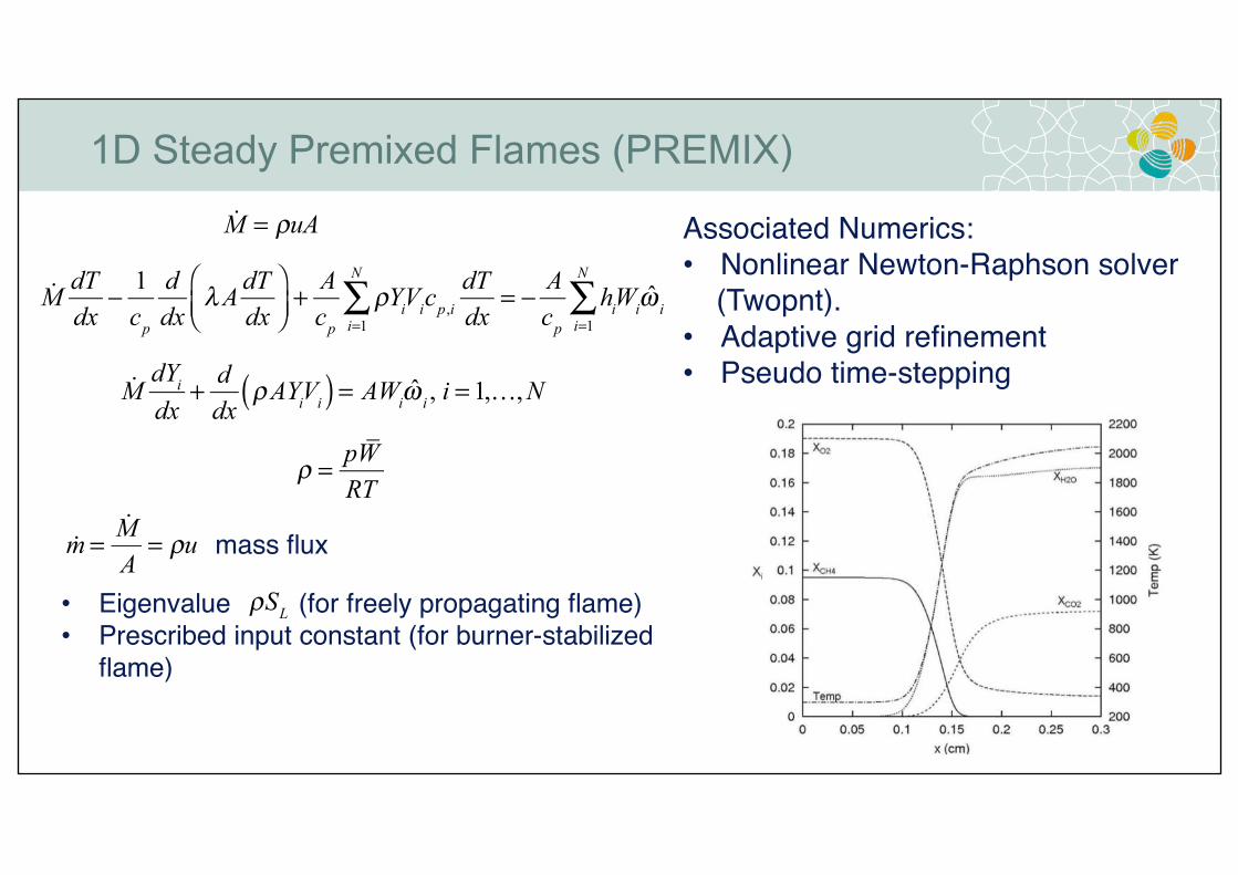
1D Steady Premixed Flames (PREMIX)

!MdT

dx−

1

cp

d

dxλA

dT

dx

⎛⎝⎜

⎞⎠⎟+

A

cp

ρYiV

ic

p,i

dT

dxi=1

N

∑ = −A

cp

hiW

iω̂

ii=1

N

∑

Associated Numerics:

• Nonlinear Newton-Raphson solver

(Twopnt).

• Adaptive grid refinement

• Pseudo time-stepping

mass flux

!M = ρuA

!MdY

i

dx+

d

dxρAY

iV

i( ) = AW

iω̂

i, i = 1,…, N

ρ =

pW

RT

!m =

!M

A= ρu

• Eigenvalue (for freely propagating flame)

• Prescribed input constant (for burner-stabilized

flame)

ρS

L

Counterflow Nonpremixed Flames – Potential Flow

′f =u

u∞

V = ρv

dV

dz+ 2aρ ′f = 0

d

dzµ

d ′f

dz

⎛⎝⎜

⎞⎠⎟−V

d ′f

dz+ a ρ∞ − ρ ′f( )

2⎡⎣⎢

⎤⎦⎥= 0

−d

dzρY

iV

i( )−VdY

k

dz+Wω̂

ii= 0, i = 1,…, N

d

dzλ

dT

dz

⎛⎝⎜

⎞⎠⎟− c

pV

dT

dz− ρY

iV

ic

p,i

dT

dzi=1

N

∑ − hiW

ii=1

N

∑ ω̂i= 0

Associated Numerics:

• Nonlinear Newton-Raphson solver

(Twopnt).

• Adaptive grid refinement

u∞= ar, v

∞= −2az ; a = −

1

2

∂v∞

∂z(given or eigenvalue)

Puri, Seshadri, Smooke, Keyes, CST 56 (1987)

Counterflow Nonpremixed Flames – Oppdif

∂

∂xρu( )+

1

r

∂

∂rρvr( ) = 0

Associated Numerics:

• Nonlinear Newton-Raphson solver

(Twopnt).

• Adaptive grid refinement

Lutz, Kee, Grcar, Rupley SAND96-8243 (1997)Continuity:

Key similarity assumption (von Karman)

G x( ) = −

ρv

r, F x( ) =

ρu

2

G x( ) =dF x( )

dxContinuity:

Eigenvalue:

H =1

r

∂p

∂r= constant

dH

dx= 0

⎛⎝⎜

⎞⎠⎟

Radial momentum:

H − 2d

dx

FG

ρ⎛⎝⎜

⎞⎠⎟+

3G2

ρ+

d

dxµ

d

dx

G

ρ⎛⎝⎜

⎞⎠⎟

⎡

⎣⎢

⎤

⎦⎥ = 0

Unsteady Opposed Flow Flames - OPUS

ρ

ptot

∂p

∂t−ρ

T

∂T

∂t− ρW

1

Wi

∂Yi

∂ti=1

N

∑ +∂

∂xρu( )+ 2ρV = 0

Associated Numerics:

• Differential-algebraic equations

(DAE) solver (DASPK)

• Compressible flow formulation

with index reduction

Im, Raja, Kee, Petzold, CST (2000)

ρ∂V∂t

+ ρu∂V∂x

+ ρV2 −

∂∂x

µ∂V∂x

⎛⎝⎜

⎞⎠⎟+ H = 0

Eigenvalue:

H (t) =1

r

∂p

∂r

dH

dx= 0

⎛⎝⎜

⎞⎠⎟

Mixing Layer

ϕ(t), T(t), V(t)

ϕ(t), T(t), V(t)

L

ρcp

∂T

∂t+ ρc

pu∂T

∂x−

∂∂x

λ∂T

∂x

⎛⎝⎜

⎞⎠⎟−∂p

0

∂t− u

∂p

∂x+ ρY

iV

ic

p,i

∂T

∂xi=1

N

∑ + hiW

ii=1

N

∑ ω̂i= 0

P = p

0(t)+ p(t,r)+

1

2H (t)r 2

+O(Ma4 )

ρ∂Y

i

∂t+ ρu

∂Yi

∂x+

∂

∂xρY

iV

i( )−W

iω̂

i= 0

ρ∂u

∂t+ ρu

∂u

∂x+∂p

∂x− 2µ

∂V∂x

−4

3

∂∂x

µ∂u

∂x−V

⎡

⎣⎢

⎤

⎦⎥

⎛

⎝⎜⎞

⎠⎟= 0

Compressible treatment

C.K. Law, Combustion Physics (2006)

The Strain Rate – Various Definitions

The Strain Rate

- For potential (Hiemenz) flow

u∞ =ax 2-D slot jet

ar round jet

⎧⎨⎩

,

v∞ = −2az ⇒ a = −1

2

∂v∞

∂z

- For opposed-jet (plug) flow

a =1

r

∂∂r

ru( ) at flame

- Approximate formula

a =V

O+V

F

L

a =2V

O

D1+

VF

ρF

VO

ρO

⎛

⎝⎜⎜

⎞

⎠⎟⎟

(Seshadri &Williams)

a ~1

Da(Damkohler number)

a ↑⇒ Da =residence time

chemical time↓⇒ Extinction

a is uniquely related to χ

Smooke

Oppdif

The Scalar Dissipation Rate

Alternatively, the flow time scale can be characterized by the scalar dissipation rate:

Elemental mass fraction

Equilibrium →

← Frozen

1

Nj ij j

j i

i i

m a WZ Y

m W=

= =å: species index ( 1, , )

: element index (C, H, O)

i i N

j

= !

( )C C H H O,O O O

C,F C H,F H O,O O

2 / 0.5 / /

2 / 0.5 / /

Z W Z W Z Z WZ

Z W Z W Z W

+ + -

=+ +

Bilger’s mixture fraction

χ = 2D ∇Z

2

[s−1

]

χ

st= 2D ∇Z

st

2

[s−1

]

The scalar dissipation rate

At the stoichiometric mixture fraction

χ

ig

-1

The Conserved Scalar Variable and

Flamelet Model Mixture Fraction Variable for a Multicomponent System

(Warnatz et al.) for C/H/O system

1

Nj ij j

j i

i i

m a WZ Y

m W=

= =å

: species index ( 1, , )

: element index (C, H, O)

i i N

j

= !

Define the elemental mass fraction

ρ∂Z

∂t+ ρu

j

∂Z

∂xj

−∂∂x

j

ρD∂Z

∂xj

⎛

⎝⎜

⎞

⎠⎟ = 0

ρ∂Y

i

∂τ= ρ

χ

2

∂2Yi

∂Z 2+ w

i if ρD ≠ f Z( )( )

χ = 2D ∇Z

2

Y

iZ ,χ( )

Flame Ignition/Extinction Study

Arc-length continuation (Giovangigli and Smooke, CST 1987)

Repeated restart of calculations with

incremental change in strain rates.

A flame-controlling continuation (Nishioka et al., C&F

1996)

Kee, Miller, Evans, Dixon-Lewis, 22nd Symp. (1988)

Nishioka, Law, Takeno, C&F (1996)

Scalar variables (T or Yi) used as a

controlling parameter.

Quantitative predictions of

ignition/extinction limits.

Applicable to premixed flames

NTC Behavior & Complex S-Curves

Farooq et al.,

https://ccrc.kaust.edu.sa/aramco/Pages/isn.aspx

Complex bifurcation behavior is manifested as

multiple turning points in the steady phase diagram.

Each turning point involves specific chemical

(exponential) nonlinearity.

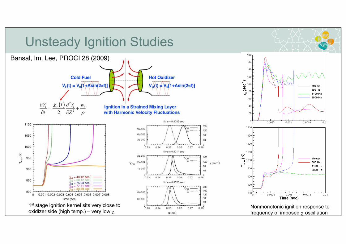
Unsteady Ignition StudiesBansal, Im, Lee, PROCI 28 (2009)

1st stage ignition kernel sits very close to

oxidizer side (high temp.) – very low cNonmonotonic ignition response to

frequency of imposed c oscillation

• Combustion dynamics is highly nonlinear due to large activation energy.

• Damköhler number serves as a determining parameter for combustion state.

• Steady vs. unsteady representations of combustion phenomena– Go/no-go is often sufficient for practical criteria

– Transient dynamics is needed to design combustion systems (ignition in engines)

• Theoretical models need not be physically realistic to be good.– Large activation energy, flame sheet limit

– Darrieus-Landau model with infinitely think flame front

– Constant density diffusive thermal model

• For simple flames, first principle continuum simulations can incorporate all detailed

physical/chemical parameters– Fidelity is subjected to the accuracy of thermo-chemistry and chemical kinetic, transport models

• Canonical flame studies are valuable for cross-validation of quantitative prediction.

This is an essential step before moving into complex turbulent combustion systems.

Summary

References

Kee, R. J., Coltrin, M. E., Glarborg, P., Chemically Reacting Flow: Theory

and Practice, Wiley, 2003.

Law, C. K., Combustion Physics, Cambridge University Press (2006).

Law, C. K. and Sung, C. J., Prog. Energy Combust. Sci., v. 26, p. 459 (2000).

Liñán, A., Acta Astronautica, v. 1, p. 1007 (1974).

Liñán, A. and Williams, F. A., Fundamental Aspects of Combustion, Oxford

University Press (1993).

Poinsot, T. and Veynante, D., Theoretical and Numerical Combustion, 2nd

ed., Edwards (2005).

Sivashinsky, G. I., Ann. Rev. Fluid Mech., v.15, p.179 (1983).

Williams, F. A., Combustion Theory, 2nd ed., Addison-Wesley (1985).