DUTCH, GERMAN, AND ENGLISH HOUSING

BUBBLES IN THE 21TH CENTURY

AN EMPIRICAL INVESTIGATION OF EXPLOSIVE BEHAVIOR IN HOUSING MARKETS IN

ORDER TO DETECT AND DATE-STAMP HOUSING BUBBLES

F.J.J. Cornelissen, LL.M.

Master thesis Financial Economics

Radboud University Nijmegen

Supervisor: S.C. Füllbrunn, PhD

i

ABSTRACT This study tries to determine whether housing bubbles existed in three European housing

markets (the Dutch, German, and English) several years prior to, during, and directly after the

recent global financial crisis. Furthermore, it aims to detect exactly when any bubbles in these

markets started and ended. In order to achieve these goals, this study uses empirical methods,

recently developed by Phillips, Wu, and Yu (2011) and Phillips, Shi, and Yu (2012), that look at

explosive behavior in house prices by applying sophisticated unit root tests. These yielded some

interesting results. While many bubbles were found in the Dutch housing market, the most

surprising results was that a bubble existed between April 2011 to September 2013. Conversely,

the German housing market was stable prior to and during the crisis but has developed a bubble

since the third quarter of 2012. The English housing market exhibited a bubble between June

2006 and January 2008 but, surprisingly, showed no signs of bubbles since. As this study will

argue, the empirical methods used to pinpoint the start and ending of bubbles can also be used

as a real-time monitoring instrument to detect housing bubbles as they form, providing policy

makers with a valuable early warning system.

Keywords: housing market bubbles, house prices, rent, right-tailed unit root tests,

Augmented Dickey-Fuller tests, date-stamping bubbles, real-time monitoring,

early warning system.

ii

CONTENTS

Abstract ................................................................................................................................................................................... i

Contents ................................................................................................................................................................................. ii

1. Introduction ................................................................................................................................................................ 1

1.1 Bubbles in European housing markets .................................................................................................. 1

2. Literature review ...................................................................................................................................................... 3

2.1 An overview of alleged bubbles ................................................................................................................ 3

2.1.1 Dutch bubbles ......................................................................................................................................... 3

2.1.2 German bubbles ..................................................................................................................................... 4

2.1.3 English bubbles ...................................................................................................................................... 6

2.2 Potential effects of housing market bubbles ....................................................................................... 6

2.3 Defining a bubble ............................................................................................................................................ 7

2.4 Fundamental value ......................................................................................................................................... 8

2.4.1 Income ....................................................................................................................................................... 9

2.4.2 Inflation, demographics, interest.................................................................................................... 9

2.4.3 Rent .......................................................................................................................................................... 10

2.5 Rational bubble theory .............................................................................................................................. 11

2.5.1 Fundamental value ............................................................................................................................ 11

2.5.2 Rational bubbles ................................................................................................................................. 13

2.6 Irrationality and bubbles .......................................................................................................................... 14

2.7 Research questions ..................................................................................................................................... 15

3. Research Method ................................................................................................................................................... 17

3.1 Statistical method: finding evidence of a bubble ............................................................................ 17

3.1.1 Variance bounds test ........................................................................................................................ 17

3.1.2 Explosive autoregressive behavior ............................................................................................. 17

3.1.3 Forward recursive autoregressive test ..................................................................................... 19

3.2 A method of date-stamping bubbles .................................................................................................... 21

3.2.1 A bubble within the sample ........................................................................................................... 21

3.2.2 Date-stamping multiple bubbles ................................................................................................. 22

3.3 Real-time monitoring ................................................................................................................................. 24

3.4 Data .................................................................................................................................................................... 25

4. Empirical testing and results ............................................................................................................................ 27

4.1 Empirical testing for bubble presence ................................................................................................ 27

4.1.1 -tests ............................................................................................................................................ 27

4.1.2 Forward recursive -test ....................................................................................................... 28

iii

4.2 Date stamping ............................................................................................................................................... 29

4.2.1 Forward recursive -test ....................................................................................................... 29

4.2.2 Backward recursive -test ................................................................................................. 32

4.3 Real-time monitoring ................................................................................................................................. 34

5. Discussion ................................................................................................................................................................. 36

6. Conclusion ................................................................................................................................................................ 39

Bibliography ...................................................................................................................................................................... 40

Appendix A: Bubble forms ........................................................................................................................................... 45

Appendix B: Time series’ graphs ....................................................................................................................... 46

1

1. INTRODUCTION

1.1 BUBBLES IN EUROPEAN HOUSING MARKETS In recent years, price developments on European housing markets have been topic of hot debate.

News articles often report on house price bubbles, whose existence is normally regarded as a

fact of common knowledge. On August 30, 2014, The Economist stated: ‘House prices in Europe

are losing touch with reality again’. Furthermore, it concludes that of twenty-three property

markets tested, nine are overvalued by at least 25%, six of which are European. Overvaluation is

defined as a positive deviation from a price-ratio’s historic average.

On the Dutch housing market specifically, the Financial Times reported on August 25, 2013, ‘that

the Dutch housing market is deflating, as prices were too high’. On the downgrading of the

Netherlands’ credit rating by Standard & Poor’s, The Economist declared at November 29, 2013:

‘[t]he chief culprit, everyone agrees, is a massive housing bubble early in the last decade’. Der

Spiegel at March 20, 2013: ‘The Netherlands is still one of the most competitive countries in the

European Union, but now that the real estate bubble has burst, it threatens to take down the

entire economy with it.’1 Figure 1 shows that house prices did indeed steeply rise from the

second half of the 1990s and started falling in 2008.

This thesis aims to investigate what many news articles so casually assume: did housing market

bubbles exist in Europe in the last decade and when did they occur? It will apply modern

econometric research methods to find answers to these questions. In order to get a

comprehensive result, while being able to apply several methods, this thesis necessarily focuses

on three countries in the 2000s and 2010s: the Netherlands, England, and Germany. These

countries are chosen partly because of the availability of data on their housing markets. Also, as

we will see below, there was at one point consensus among economists about the presence of a

bubble for the Dutch, English and German housing markets. Therefore, the results of this

research are also an assessment of methods used and opinions given by economists on these

markets. That assessment may add to the relevance of this thesis.

The importance of detecting housing market bubbles stands in sharp contrast to the inability of

economists to agree on whether particular bubbles exist (section 2.1). Therefore, this thesis

aims to add some clarity to theoretical and methodological issues concerning bubble tests, and

to establish if and when bubbles existed on the Dutch, German, and English housing markets. To

this end, other literature on the definition and nature of housing bubbles will be discussed next.

Then, the theoretical and methodological framework of this study are outlined, empirical tests

are performed.

This study detects housing bubbles by comparing house price movements to movements in rent.

It asserts that the fundamental value of houses depends on rents. Explosive behavior of house

prices constitutes a bubble if it is not caused by a simultaneous explosiveness of rents. Using

several right-tailed unit root tests to determine whether either house prices or rents behave

explosively, this study will determine if bubbles exist in housing markets and, if so, when they

1 Translation of this originally German article obtained from: http://www.spiegel.de/international/europe/economic-crisis-hits-the-netherlands-a-891919.html, retrieved at April 25, 2014.

2

started and ended (if at all). Also, a new way to monitor housing markets in real time is

proposed.

It is also important to note what this thesis does not aim to do. It does not explain why or how

bubbles occur. It will not give any policy advice, other than advice on how to better detect

market bubbles. If a bubble is detected, this thesis will not explain what its consequences would

be, or whether a ‘soft landing’ is possible or desirable.

3

2. LITERATURE REVIEW

2.1 AN OVERVIEW OF ALLEGED BUBBLES

2.1.1 DUTCH BUBBLES When looking at a visual representation of Dutch housing prices (Figure 1), one could easily

assume that a bubble occurred, and that it reached its height in 2008. While the alleged bubble

in the Dutch housing market apparently formed and subsequently collapsed, consensus in

economic literature was lacking. As late as 2010 there was and had been no housing market

bubble according to many economists despite many disturbing signs (Knibbe, 2010, pp. 106-

107). Real house prices had already fallen by 8% in two years’ time, while they had risen

between 1986 and 2007 by about 150% (Knibbe, 2010, p. 106).

FIGURE 1: DUTCH HOUSE PRICE INDEX (2010=100), CONTAINING 221 MONTHLY OBSERVATIONS, FROM JANUARY 1996 TO MAY 2014. DATA

SOURCE: STATLINE, STATISTICS NETHERLANDS (MORE INFORMATION IN SECTION 3.4).

Many researchers use an error correction model (ECM) to determine whether house prices are

overvalued. Such a model consists of two (main) equations, representing a long-term

equilibrium and short-term price adjustments. In the long run, the level of house prices is

modeled to depend on one or more fundamental variables (level of income, rent etc., section

2.4). However, in the short run, the change in house prices depends on changes in fundamentals,

previous house price changes and the deviation of actual house prices from their long-term

equilibrium.

Using such a model, Francke (2010, p. 17) asserts that Dutch house prices were not overvalued

as of 2009. The CPB Netherlands Bureau for Economic Policy Analysis estimated a 10 percent

overvaluation of house prices in 2003 (2005, p. 29) that shrunk to approximately 0 percent in

2007 (2008, p. 7). According to the OECD, there was a 20.4 percent house prices overvaluation

in 2004 (2005, p. 136).

At the same time, the IMF found a gap of 30 percent between actual and fundamental house

prices that cumulated between 1997 and 2007 (2008, p. 113), contradicting the CPB’s

40

60

80

100

120

Dutc

h h

ouse

price

ind

ex

Jan 1996 Sep 1999 May 2003 Jan 2007 Sep 2010 May 2014

4

assessment. In 2009 however, the International Monetary Fund (2009, p. 10) states that ‘[t]he

housing market (…) does not appear out of kilt (…)’. Similarly, in 2011 IMF’s Executive Director

for the Netherlands concludes that ‘house prices seem to be in line with fundamentals’

(International Monetary Fund, 2011).

Dreger and Kholodilin (2013, p. 13) investigated large samples of housing market data on 12

OECD countries and detected no bubbles on the Dutch housing market between the third

quarter of 1978 to the last quarter of 2009. This finding contradicts the assessments mentioned

above by the CPB, the OECD, and the IMF.

In its 2014 edition of the Economic Survey, the OECD (2014, p. 11) asserted that Dutch house

price-to-rent and house price-to-income ratios are still above their long-term averages in the

last quarter of 2013 (by 5% and 20%) and warns that house prices could therefore continue to

fall. There is and has been no agreement among economists whether the Dutch housing market

experienced one or more bubbles in the last two decennia and when they occurred.

2.1.2 GERMAN BUBBLES Unlike the Dutch housing market, the German housing market seemed a clear-cut case for most

of the 2000s. German real house prices had been quite stable since 1999. According to Kofner

(2014), this stability is due to the tenure structure of the German housing market, which is

relatively unique for a developed country. In 2012, only 53.3 percent of Germany’s population

lives in owner-occupied houses. 2 The academic consensus seems to have been that no

overvaluation of German house prices had existed. There are few publications on house prices

during this stable period. This is probably due to a publication bias: few people are willing to

publish articles or reports on stationary markets and the absence of a bubble. IMF Staff reports

do not explicitly tell German authorities not to worry about housing price developments. Also,

researchers will often only try to detect a bubble if they hypothesized it is really there. Dreger

and Kholodilin (2013, p. 13) did look for housing market bubbles in Germany but found none in

a period from 1995 to 2009.

In recent years, however, German house prices have been increasing (Figure 2) and this increase

raises the question whether a bubble is forming. The Bundesbank, having a reputation for

conservatism, suggests in its Monthly Report in October 2013 that lax monetary policy by the

European Central Bank may lead to an inflation of house prices. The report estimates an

overvaluation of house prices of 5 to 10 percent in urban areas and even 20 percent in

particularly attractive cities but found no substantial overvaluation in the German property

market as a whole (Bundesbank, 2013, pp. 13, 28).

Thus far, German economists seem to agree with their national bank. Just et al. (2013, p. 35)

found no ‘Blasenbildung’ in the German property market and Feld et al. (2014, p. 3) state: ‘Von

Überhitzung derzeit keine Spur.‘ Chen and Funke (2013, pp. 12-13) also found no bubble up until

the last quarter of 2012. Tschekassin (2014) even points out that two important indicators, the

price-to-rent ratio and the price-to-income ratio, were still below their long-term averages in the

last quarter of 2013. The OECD (2014, p. 12) agrees that with the Bundesbank that although

some local overvaluation may exist, there is no bubble in the housing market as a whole. The

IMF (2014, pp. 25-26) also agrees with the assessment of the Bundesbank and the OECD, but it

2 Eurostat 2012, http://appsso.eurostat.ec.europa.eu/nui/show.do?dataset=ilc_lvho02&lang=en. Retrieved September 11, 2014. For Switzerland, this number is even lower: 43.8%.

5

advises German authorities to carefully monitor the housing market in the near future (p. 36):

‘While concerns about a housing bubble are premature, preparations against it are not.’

FIGURE 2: GERMAN HOUSE PRICE INDEX (2010=100), CONTAINING 55 QUARTERLY OBSERVATIONS, FROM 2000Q1 TO 2013Q3. DATA

SOURCE: DESTATIS, GERMAN FEDERAL STATISTICS OFFICE (MORE INFORMATION IN SECTION 3.4).

In short, no-one believes a bubble was present on the German housing market in recent years,

even though prices have risen (Figure 2). However, the increased house prices did prompt the

IMF to advice German authorities to closely monitor further developments.

FIGURE 3: ENGLISH HOUSE PRICE INDEX (2010=100), CONTAINING 113 MONTHLY OBSERVATIONS, FROM JANUARY 2005 TO MAY 2014. DATA SOURCE: OFFICE OF NATIONAL STATISTICS (MORE INFORMATION IN SECTION 3.4).

95

100

105

110

Germ

an h

ouse

price

ind

ex

2000Q1 2002Q2 2004Q3 2006Q4 2009Q1 2011Q2 2013Q3

80

90

100

110

120

En

glis

h h

ou

se p

rice in

de

x

Jan 2005 Nov 2006 Oct 2008 Aug 2010 Jul 2012 May 2014

6

2.1.3 ENGLISH BUBBLES Economists did find bubbles in an English housing market that has undergone large shifts in

house prices in recent years (Figure 3). Fry (2009) found that bubbles comprised 30 to 40

percent of English house prices between 2002 and 2007. And Dreger and Kholodilin (2013, p.

13) detected a bubble in the aggregate UK housing market in roughly the same period (2002Q2

to 2007Q2). An analysis ordered by the European Commission concluded that late in 2008,

prices were (much) higher than any fundamentals could justify (Kuenzel & Bjørnbak, 2008).

Recently, the IMF (2014, p. 26) stated that the United Kingdom, including England, is at (high)

risk of experiencing a sharp reduction in house prices. It also notes that house prices are

increasing rapidly. The IMF does not use the terms ‘bubble’ or ‘overvaluation’, but it strongly

seems that this is exactly what it has found and is warning for. Along the same lines, the

Governer of the Bank of England stated during a hearing of the Treasury Committee of the House

of Commons that the housing market contains great risks to the UK economy, especially because

house prices are ‘biased upwards’ (Treasury Committee, 2014), which seems to be a euphemism

for a bubble.

On the English and UK housing markets, a general consensus exists that a bubble existed up until

2007 or 2008 (at least) and that the recent increase in house prices also indicates a bubble.

2.2 POTENTIAL EFFECTS OF HOUSING MARKET BUBBLES ‘Prior to the global recession of 2008-2009 and the associated disruptions in financial markets, asset price

bubbles were often considered as a sideshow to macroeconomic fluctuations. The global recession demonstrated

painfully that this dominant pre-crisis presumption was dangerously wrong.’ (Chen & Funke, 2013, p. 2)

The importance of detecting bubbles in the housing market cannot be overstated. The deflation

or implosion of such bubbles has large adverse effects both on the macroeconomic scale and at

the level of households (Baker, 2002, p. 12). These separate types of impact are shortly

addressed here.

When there is a housing bubble, people will want to invest more in houses because they expect

prices to rise even further. They will buy larger or more houses than they would otherwise do.

The bubble also spurs consumption in two ways. First, there is a direct effect: larger and more

houses need more furniture, carpets and other household items. Secondly, the wealth effect of

the housing bubble affects consumption indirectly. As people see their wealth accumulating

because of the rising value of their houses, they are likely to feel less need to save for the future.

Higher house prices also enable house-owning families to borrow more as they can use their

home equity to secure loans. This money is spend on consumption. Case et al. (2005, p. 1249)

found ‘strong evidence that variations in housing market wealth have important effects upon

consumption’ and concluded that the housing market appears to be more important than the

stock market in influencing consumption.

Large though the effects of a collapsing housing bubble on the macroeconomic scale may be, for

individual households, the impact can be even more severe. As the home is often a family’s most

important asset, a sudden decline in its value greatly affects the household’s wealth. As long as it

does not sell the house, and does not immediately need the wealth represented by the house, no

problems may occur. However, if people planned to liquefy their wealth by selling or

remortgaging in order to finance their retirement, their retirement income will be much lower.

Furthermore, if people are forced to move because of a divorce or because of their jobs, they

7

may be left with large debts as their mortgage loan is larger than the market price of their house.

If this effect prevents people to be able to move for new jobs, it also leads to inefficient job

markets and possibly to more unemployment.

Reinhart and Rogoff (2008) investigated a selection of 18 financial crises in different countries

and found that a large rise in housing prices almost always preceded a crisis. The housing

market may therefore be a contributing factor in a certain state of the economy that leads to a

crisis. This relation is also described by Kindleberger and Aliber (2005, p. 117). Even if no such

causal relationship exists, housing prices may serve as an early warning of an approaching

financial crisis.

Local government income depends heavily on house prices, because of real property tax.3 A

collapsing housing market bubble could significantly affect the income of Dutch and German

municipalities, and England’s districts.

2.3 DEFINING A BUBBLE There is no one answer to what a bubble in asset prices is exactly. Kindleberger and Aliber

(2005, p. 29) give a very broad definition and state that a bubble is ‘an upward price movement

over an extended period of fifteen to forty months that then explodes’. The esteemed economist

Robert J. Shiller, who together with Fama and Hansen received a Nobel Prize in 2013 ‘for their

empirical analysis of asset prices’ states:

‘I define a speculative bubble as a situation in which news of price increases spurs investor enthusiasm, which

spreads by psychological contagion from person to person, in the process amplifying stories that might justify

the price increases and bringing in a larger and larger class of investors, who, despite doubts about the real

value of an investment, are drawn to it partly through envy of others’ successes and partly through a gambler’s

excitement.’ (Shiller, 2005, p. 2)

Regrettably, both widely used definitions are not suited to this thesis. Kindleberger and Aliber’s

encompasses more than what is an asset price bubble. When market agents expectations on

future cash flows arising from an asset rise, than the price of that particular asset should also

rise. A sudden negative change in expectations then could adversely and instantly affect the

price of that asset. For example, the unexpected discovery of large quantities of easily mineable

gold would undoubtedly cause a large drop in gold prices. This does not mean that rising gold

prices prior to the drop constitute a bubble. In this case, the “explosion” of the price movement is

caused by fundamentals. The definition given by Shiller on the other hand, describes a

psychological process that is hardly testable at the housing market scale. More importantly, his

definition seems to preclude the possibility that agents investing in bubble markets might do so

rationally. They may invest when they expect the bubble to expand even more.

An empirically testable and conceptually sound definition of an asset price bubble can be

deduced from the following statement by Joseph E. Stiglitz:

‘[I]f the reason that the price is high today is only because investors believe that the selling price will be high

tomorrow – when ‘fundamental’ factors do not seem to justify such a price – then a bubble exists.’ (Stiglitz,

1990, p. 13)

3 In the Netherlands, municipalities collect Onroerendezaakbelasting pursuant to the Wet waardering onroerende zaken. The Grundsteuergesetz delegates power to German municipalities to collect Grundsteuer. In England, districts collect Council Tax in carrying out the Local Government Finance Act 1992.

8

Lind (2009, p. 81) notes that this definition does not cover the whole bubble episode and only

refers to price increases, and rejects Stiglitz’ definition. I will stick to Stiglitz’ bubble description

but suggest adding a phrase to include the period between a bubble’s collapse and the return to

fundamental value:

‘(…) then a bubble exists until the price returns to a level that is justified by those fundamentals.’

A bubble thus exists if, for a significant period of time, the price of an asset exceeds its

fundamental value. The price is not justified by its fundamentals, and the difference between

market price and fundamental value is a bubble. Some economists even allow for negative

bubbles (Siegel, 2003, p. 14). As asset price bubble can exist solely because of the belief that,

regardless of the fundamental value, an existing overvaluation will endure. This is commonly

referred to as a rational bubble. The theory of rational bubbles is central to this thesis and will

be discussed formally in section 2.5.

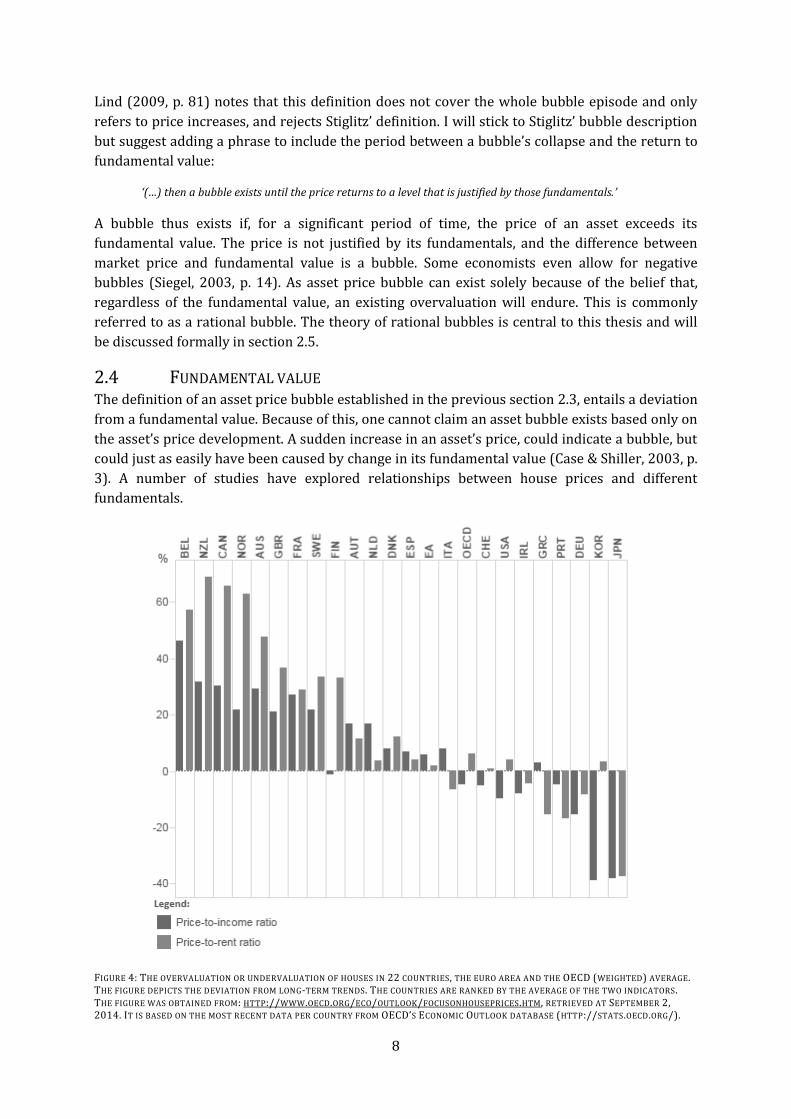
2.4 FUNDAMENTAL VALUE The definition of an asset price bubble established in the previous section 2.3, entails a deviation

from a fundamental value. Because of this, one cannot claim an asset bubble exists based only on

the asset’s price development. A sudden increase in an asset’s price, could indicate a bubble, but

could just as easily have been caused by change in its fundamental value (Case & Shiller, 2003, p.

3). A number of studies have explored relationships between house prices and different

fundamentals.

FIGURE 4: THE OVERVALUATION OR UNDERVALUATION OF HOUSES IN 22 COUNTRIES, THE EURO AREA AND THE OECD (WEIGHTED) AVERAGE. THE FIGURE DEPICTS THE DEVIATION FROM LONG-TERM TRENDS. THE COUNTRIES ARE RANKED BY THE AVERAGE OF THE TWO INDICATORS. THE FIGURE WAS OBTAINED FROM: HTTP://WWW.OECD.ORG/ECO/OUTLOOK/FOCUSONHOUSEPRICES.HTM, RETRIEVED AT SEPTEMBER 2, 2014. IT IS BASED ON THE MOST RECENT DATA PER COUNTRY FROM OECD’S ECONOMIC OUTLOOK DATABASE (HTTP://STATS.OECD.ORG/).

9

2.4.1 INCOME In studies of residential property bubbles, a common fundamental is the per capita disposable

income. The price-to-income ratio, also referred to as the affordability ratio, is a measure of

whether or not a house is within reach of the average buyer. In theory, if the ratio is too high,

buying a house is no longer attainable for prospective buyers, demand will drop and therefore

house prices decrease. In this way, the ratio is always expected to return to a long-term

(fundamental) average (Girouard, Kennedy, Noord, & André, 2006, p. 16). Figure 4 depicts the

deviation of the price-to-income ratios to long-term equilibria. According to the price-income

relationship and this method, Dutch house prices are overvalued, as are house prices in Great-

Britain and – probably – England. German house prices on the other hand are undervalued.

There is some criticism in literature on using the price-to-income ratio to look for bubbles.

Girouard et al. note a serious flaw in the measurement: the disposable income is an average of a

whole population, while buyers and sellers on the housing market have higher-than-average

incomes (2006, p. 16). Another objection is raised by Gallin (2003). He found no evidence in US

housing market data that there is a significant relationship between the level of house prices and

the level of disposable income and asserts that many tests for bubbles based on this relationship

may be inappropriate. Furthermore, André notes that tests based on the price-to-income ratio

cannot exclude that a higher ratio is caused by a higher (long-term) equilibrium (2010, p. 11).

2.4.2 INFLATION, DEMOGRAPHICS, INTEREST Brunnermeier and Julliard (2006) looked at the relationship between house prices and inflation

and found that potential home buyers base their decision to purchase a house not on the real

interest rate, but on the nominal interest rate. They attribute the influence of inflation to money

illusion, due to the fact that households compare monthly rental payments to nominal mortgage

payments.

Other fundamentals are financing conditions, such as the availability of mortgage loans, and

demographic development (André, 2010, p. 27). As populations grow, demand for homes

increases. Furthermore, household size has generally diminished over time in OECD countries,

due to larger numbers of single-parent families, and an ageing population that is increasingly

autonomous (Heyer, Le Bayon, Péléraux, & Timbeau, 2005, p. 16). These and other demand-

increasing factors affect house price level especially because of rigidities in the housing markets’

supply adjustment (André, 2010, p. 27).

It is virtually uncontested that a significant relationship between the interest rates and house

price movements exists (McQuinn & O'Reilly, 2008). Low interest rates open up the housing

markets for more households (and allow existing homeowners to be able to purchase larger

houses) as a result of cheaper mortgage loans. Also, opportunity costs for owning a house are

lower. Furthermore, a lower (nominal) interest rate, positively affects demand as it decreases

borrowing restraints for households (André, 2010, p. 19) As a result, a decrease in interest rates

stimulates demand for residential property and therefore house prices should rise. Case and

Shiller (2003, p. 312) however, found that in several US housing markets in the 1990s, house

prices did not significantly respond to changes in interest rates. They contribute this finding to

simultaneity: low interest rates stimulate the housing market, but low interest rates may be

caused by monetary easing as a response to a weak economy and housing market.

10

Shiller (2007) also mentions the construction cost of new houses as an important fundamental

that is significantly related to house prices.

2.4.3 RENT Many researches testing for housing bubbles focus on the relationship between prices and rent,

e.g.: Ambrose et al. (2013), Yiu & Lu (2012), Shi (2007), Hwang-Smith & Smith (2006), and Chan

et al. (2001). The price-to-rent ratio can be seen as the cost of owning versus renting a house

(Girouard, Kennedy, Noord, & André, 2006, p. 19). The relationship between house prices and

rent can also be interpreted as between an investment and the cash flows it generates. The

fundamental value as the present value of future cash flows is explained in detail in section 2.5.1.

Gallin studied US housing market data from 1970 to 2003 and found that a significant

relationship between rent and house prices exists (2004). The OECD found that, according to the

price-to-rent ratios, Dutch house prices are (slightly) overvalued, British house prices are

overvalued by nearly 40 percent, and German house prices are undervalued (Figure 4).

Glaeser and Gyourko (2007, pp. 17-22) argue that there is little arbitrage between owning and

renting on the housing market. First of all, the abstract notion of consumable housing units does

not exist in real life: rental property is very different from owner-occupied property. On average,

rental homes are units in buildings that house multiple households (e.g., apartments), while

owner-occupied homes are often detached houses. Furthermore, both types of homes are

located in different parts of metropolitan areas and have different quality neighborhoods. Also,

renters and owners are different types of people. Knibbe (2010, p. 109) makes the point that not

all households are able to choose between renting and buying as low income groups often do not

have access to the mortgage market. Many households therefore do not have (or make) a real

choice between renting and owning.

In spite of the observation that there is only limited arbitrage between owning and renting, this

thesis will use the price-rent relationship to model the housing markets. First of all, the link

between house prices and rent is conceptually clear (section 2.5.1). Because both rent and house

prices are housing market variables, many other fundamentals discussed here affect them

symmetrically (Brunnermeier & Julliard, 2006, p. 9) (Ambrose, Eichholtz, & Lindenthal, 2013, p.

16). For example, higher disposable incomes are likely to positively affect both rents and

housing prices. Similarly, on a 30 percent increase in US real house prices between 1995 and

2002, Baker states:

‘The fact that rents had risen by less than 10 percent in real terms should have provided more evidence to

support the view that the country was experiencing a housing bubble. If there were fundamental factors driving

the run-up in house sale prices they should be having a comparable effect on rents.’ (Baker, 2008, p. 74)

Furthermore, even though there may be limited arbitrage between owning and renting, a house

can also be viewed as an investment that requires certain future cash flows (rental income) to

justify its price (section 2.5.1). Much literature on asset price bubbles refers (primarily) to stock

market bubbles. The fundamental value is always determined by the present value model,

whereby the sum of discounted expected future dividends from that stock constitutes its

fundamental value. For the housing market, the fundamental value of houses is similarly

determined by their strand of expected future cash flows. Instead of dividends, houses generate

rental income. As Hwang-Smith and Smith (2006, p. 8) argue, the implicit cash flow from an

owner-occupied house, are the rental payments that would have to be made if the house were

rental property. The fundamental value and market value of a house are perhaps unclear for

11

market agents. Real property markets are characterized by infrequent, privately negotiated

deals in which whole, unique assets are traded. In this type of market, it is difficult to know at

any given time the precise market value of any given real estate asset (Geltner, Miller, Clayton, &

Eichholtz, 2007, p. 272). In these aspects, the real estate market differs from stock markets.

Every listed share always has a clear market price, as shares, unlike houses, are homogeneous

goods that are traded frequently and publicly. House prices have been shown to be somewhat

forecastable (Case & Shiller, 1989), which is probably due to the fact that entering and exiting

the housing market is costly (Shiller, 2005, p. 14).

2.5 RATIONAL BUBBLE THEORY

2.5.1 FUNDAMENTAL VALUE As mentioned in section 2.4, this paper explores the relationship between actual house prices as

opposed to fundamental house prices, determined by rent. The fundamental value of houses is

expressed mathematically according to the present value model, as demonstrated by Homm and

Breitung (2012, pp. 200-201) for stocks. By definition, the following standard no-arbitrage

condition must be true for the rate of return on any asset:

Equation 1

,

where is the rate of return on holding the asset at time , denotes the asset price at time

and is the return (pecuniary or otherwise) on the asset at time .4

As Brancaccio (2005, p. 27) notes, Equation 1 is only an accounting definition. In order to

produce the final present value model equation, three assumptions have to be made that can be

represented schematically (Figure 5).

FIGURE 5: THREE ASSUMPTIONS OF THE PRESENT VALUE MODEL.

4 This timing assumption is a convention in finance literature. Holding a stock gives a claim to next period’s dividend but not to this period’s dividend. By contrast, Blanchard and Watson (1982), who for the first time described mathematically how rational bubbles can exist, do not adhere to this convention and

assert that

.

Present Value Model

Constant expected return on asset R

ASSUMPTION I

Constant intertemporal preferences and risk

neutrality

ASSUMPTION II At any given time, all agents have the same information

and have rational expectations

ASSUMPTION III Transversality condition

12

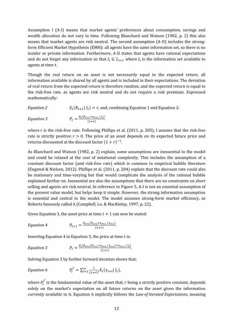
Assumption I (A-I) means that market agents’ preferences about consumption, savings and

wealth allocation do not vary in time. Following Blanchard and Watson (1982, p. 2) this also

means that market agents are risk neutral. The second assumption (A-II) includes the strong-

form Efficient Market Hypothesis (EMH): all agents have the same information set, so there is no

insider or private information. Furthermore, A-II states that agents have rational expectations

and do not forget any information so that , where is the information set available to

agents at time .

Though the real return on an asset is not necessarily equal to the expected return, all

information available is shared by all agents and is included in their expectations. The deviation

of real return from the expected return is therefore random, and the expected return is equal to

the risk-free rate, as agents are risk neutral and do not require a risk premium. Expressed

mathematically:

Equation 2 ( ) , and, combining Equation 1 and Equation 2:

Equation 3 ( )

( ).

where is the risk-free rate. Following Phillips et al. (2011, p. 205), I assume that the risk-free

rate is strictly positive: . The price of an asset depends on its expected future price and

returns discounted at the discount factor ( ) .

As Blanchard and Watson (1982, p. 2) explain, some assumptions are inessential to the model

and could be relaxed at the cost of notational complexity. This includes the assumption of a

constant discount factor (and risk-free rate) which is common in empirical bubble literature

(Engsted & Nielsen, 2012). Phillips et al. (2011, p. 204) explain that the discount rate could also

be stationary and time-varying but that would complicate the analysis of the rational bubble

explained further on. Inessential are also the assumptions that there are no constraints on short

selling and agents are risk neutral. In reference to Figure 5, A-I is not an essential assumption of

the present value model, but helps keep it simple. However, the strong information assumption

is essential and central to the model. The model assumes strong-form market efficiency, as

Roberts famously called it (Campbell, Lo, & MacKinlay, 1997, p. 22).

Given Equation 3, the asset price at time can now be stated:

Equation 4 ( )

( ).

Inserting Equation 4 in Equation 3, the price at time is:

Equation 5 ( ( ) )

( ).

Solving Equation 3 by further forward iteration shows that:

Equation 6 ∑

( ) ( ),

where

is the fundamental value of the asset that, being a strictly positive constant, depends

solely on the market’s expectation on all future returns on the asset given the information

currently available to it. Equation 6 implicitly follows the Law of Iterated Expectations, meaning

13

that if , one cannot predict at time , when available information is restricted to the set

, what the forecast error one would make having (Campbell, Lo, & MacKinlay, 1997, p. 23).

The fundamental value therefore only depends upon information that is currently available.

Equation 6 is only a unique solution to Equation 3 when the transversality condition (A-III)

holds (Blanchard & Watson, 1982, p. 7):

Equation 7 .

( ) / , so that

Equation 8

.

Equation 7 means that the present value of the asset price at an infinitely far away future period,

is zero. This value of the asset depends on expected returns from that future date onward

(Equation 6). The transversality condition therefore requires cash flows to grow at a lower rate

than .

In short, if the three main assumptions depicted in Figure 5 hold, an asset’s actual price

represents its fundamental value.

2.5.2 RATIONAL BUBBLES For a long time economists took any deviations of actual prices from goods’ fundamental values,

when observed, as evidence of irrationality. Blanchard and Watson (1982, p. 1) asserted for the

first time that this is a non sequitur as the argument precluded the possibility of a rational

bubble. This is a bubble rational agents would buy in to in order to sell the asset in the future

when it is (rationally) expected to be at least equally overvalued.

In order for a bubble to form in this present value framework, no irrationality need be

introduced. Markets can still be efficient and market agents still carry rational expectations (A-

II). For a bubble to be able to exist, relaxing A-III suffices.

Without the transversality condition of Equation 7, is not the only price that solves equation

(1). A bubble component can be introduced. Consider for example a process ( ) with the

property

Equation 9 ( ) ( ) .

Evidently, adding the bubble component to the fundamental asset price

results in another

solution to Equation 3:

Equation 10 , where ,

so that there can be no negative bubble. When agents can freely dispose of an asset, rationality

implies that cannot be negative (Blanchard & Watson, 1982, p. 7). Applying the Law of

Iterated Expectations to Equation 9, the expected bubble component at a future time can be

described as

Equation 11 ( ) ( ) .

If is negative at any time, it would grow at a rate of each period and as , ( )

, implying a negative asset price somewhere in the future (Homm & Breitung, 2012, p. 201).

14

It must then be true as Phillips et al. (2011, p. 205) point out, that ( ) , so the bubble is

a submartingale and explosive in behavior.

If there was no bubble, would equal

. If there is a bubble however, it must be expected to

grow at a rate of at least . This means that future asset prices are expected to grow at a rate

(Equation 7). This makes intuitive sense: no-one would be willing to buy an overpriced

asset if he did not believe that it would remain overpriced. Furthermore, the added investment

in the overpricing should at least be expected to grow at a rate for which it could either be

borrowed or could generate income elsewhere. If investors believe that overpriced assets will

increase at least at rate , and subsequently invest in property, the actual asset prices will indeed

rise and complete the loop of a self-fulfilling prophecy (Homm & Breitung, 2012, p. 201). The

model thus shows the workings of the ‘Greater Fool Theory’: the last buyer is always (rationally)

counting on the greater fool to sell the asset to (Kindleberger & Aliber, 2005, p. 13).

The rate at which the bubble component grows, should not exceed however, as Equation 9

shows. If ( )

, then investments would grow to profit from a return higher than

inflating the bubble component until Equation 9 holds again. The bubble ( ) is commonly

referred to as ‘rational’ because, as shown here, it is entirely consistent with A-II: agents have

rational expectations (Campbell, Lo, & MacKinlay, 1997, p. 258).

While conforming to Equation 9 and Equation 11, the actual bubble process may take several

forms. Some of these are discussed in detail in Appendix B: Time series’ graphs. It is important

to note that while rational bubble theory explains how a rational bubble can exist, it does not

explain how it emerges. It just assumes that a (strictly positive) bubble component is always

present (Equation 10).

2.6 IRRATIONALITY AND BUBBLES Traditionally, heterodox definitions of market bubble are quite colorful, like the one given by

behavioral economist Shiller (2005, p. 2), quoted in section 2.3. Kindleberger and Aliber (2005,

p. 39) use words like ‘speculative mania’, and ‘something close to mass hysteria’ to describe a

financial bubble.5

Heterodox economists view stock market bubbles as a result of overenthusiastic investors.

Especially when the market is in Minsky’s (1972, p. 102) words ‘euphoric’, these agents tend to

overestimate future dividends and therefore are willing to pay more for the stock than they

should. In other words, the agents behave irrationally (Brancaccio, 2005, p. 32).

In the (neoclassical) present value model, irrational investor behavior can be interpreted as a

rejection of the rational expectations and efficient market hypothesis, A-II. For a long time, a

deviation from fundamentals was defined as irrationality, until rational bubble theory was

developed. In the previous section, this reasoning was already exposed as a non sequitur

argument. Regrettably, it still pervades a part of the economic literature, and much of popular

literature (LeRoy, 2004, p. 785). For example, Hall draws this conclusion:

5 One could argue that behavioral finance, as practiced by Nobel Prize laureate Shiller, is not heterodox (anymore). For simplicity’s sake, I will adhere to the convention of calling all fields of economics ‘heterodox’ that are not neoclassical.

15

‘I reject market irrationality in favor of the hypothesis that the financial claims on firms command values

approximately equal to the discounted future returns.’ (Hall, 2001, p. 1)

In this thesis, I will focus on rational bubble theory for several reasons. There is no testable

model of a relation between agents’ irrationality and financial bubble. As the objective is to

determine whether there are or have been any bubbles in housing markets, the theory must be

testable. For the moment, heterodox economics is at best able to explain why and how a bubble

develops, but cannot tell from historic data if a bubble existed in a particular period. Behavioral

finance literature in particular explores the development of psychological characteristics only in

general terms and does not compare market agents’ behavior at the beginning of a boom and at

the moment the market crashes. Therefore, it cannot explain the formation and collapse of

bubbles directly (Komáromi, 2006, p. 20). According to Blanchard, ‘old’ (heterodox) theorists

use only ‘anecdotal methodology’ (Brancaccio, 2005, p. 34).

In contrast, bubble tests based on the rational bubble model have been proven to detect bubbles

that experience shows to have been bubbles. Examples of bubbles detected by methodology

based on rational bubble theory are the 1990s NASDAQ bubble (Phillips, Wu, & Yu, 2011), the

late 1990s and early 2000s dot-com bubble in the S&P500 (Phillips, Shi, & Yu, 2012), and the

residential property market bubble in Hong Kong in the 1990s (Chan, Lee, & Woo, 2001) and the

2000s (Yiu & Lu, 2012). As Friedman (Friedman, 1966, p. 15) argued, the ‘realism’ of an

assumption is not relevant. The sole criterion on which to judge an assumption is whether the

theory works, which it does if it yields sufficiently accurate predictions. This means that using

the rational bubble theory to describe market bubbles does not require one to believe the

bubble was actually caused by rational agents and rational behavior. Even if purely rational

bubbles may seem unlikely, we can still learn from studying them (Campbell, Lo, & MacKinlay,

1997, p. 206). Behavioral finance and other disciplines may still explain why the market acted

the way it did when a ‘rational’ bubble is found. This point is best explained by the following

quote of historic economists Kindleberger and Aliber.

‘Rationality is thus an a priori assumption about the way the world should work rather than a description of the

way the world has actually worked. The assumption that investors are rational in the long run is a useful

hypothesis because it illuminates understanding of changes in prices in different markets; in the terminology of

Karl Popper, it is a ‘pregnant’ hypothesis. Hence it is useful to assume that investors are rational in the long run

and to analyze economic issues on the basis of this assumption.’ (Kindleberger & Aliber, 2005, p. 40)

2.7 RESEARCH QUESTIONS This thesis will focus on these main research questions, that will be answered for the Dutch,

German and English housing markets. First, it wil answer the question:

1. Is there any evidence for bubbles in the housing markets in the 21th century?

If the hypotheses that bubbles were and are present, are supported by empirical evidence, this

thesis will also investigate when these bubbles started and when the bubbles ended, if they

ended at all. This is captured by the following research questions:

2. If bubbles exist, when did they start and when did the bubbles end (if at all)?

Answering this question will require identifying the exact periods that markets were in bubble

territory. Next, the problem is faced of detecting a bubble while it is forming. Methods of

detecting overheating of markets in an early stage can be of great importance to policy makers.

16

This goes for housing markets especially, considering the great potential impact of bubbles as

explained in section 2.2. Therefore, I pose this research questions:

3. Is it possible to have an early warning system for housing market bubbles and

crashes?

4. If such an early warning system is conceivable, what does it say on the current

price movement in the Dutch, German, and English housing markets?

17

3. RESEARCH METHOD The theoretical framework that is described in section 2.5, can be tested in several ways. First,

the method for establishing whether or not there was a bubble must be determined. Assuming a

bubble will indeed be found, a separate method is needed to assess when it started and ended.

Finally, a real-time monitoring method will be discussed to investigate if the housing market

bubble could have been detected while it was forming.

3.1 STATISTICAL METHOD: FINDING EVIDENCE OF A BUBBLE

3.1.1 VARIANCE BOUNDS TEST The first methods used to discover bubbles, were the variance bounds tests developed by Shiller

(1981) and by LeRoy and Porter (1981). These tests, explained in more detail by Gürkaynak

(2008, pp. 170-173), are based on the assertion that the variance of the ex post rational price of

an asset (based on actual income) must in absence of a bubble be larger than the variance of the

actual price at the time (based on expected future income). This is true because an

unforecastable, mean zero error term is added to the expected incomes in equation (6) to form

actual incomes, giving this new equation:

Equation 12 ∑

( ) * ,( ) -+ ∑

( ) ,

Where is the return on the asset in period , is the error term, is the actual asset

price and represents the ex post rational price under the hypothesis that no bubble exists (i.e.,

). As the variance of can be determined by the (strictly positive) variances ( ) of

and ∑

( ) , it must be true that

Equation 13 ( ) ( ).

Shiller (1981) found that for American stock prices and dividends between 1871 and 1979, the

variance of the actual real stock price was much larger than the variance of the ex post rational

price. He used this deviation from theory to criticize the present value model. Others, however,

attributed this high and unexplained volatility to asset price bubbles (Gürkaynak, 2008, p. 171).

Using a variance bounds test for bubble detection in this way has since been rejected in

economic literature. It offers no structure on the bubble component, can offer no more than an

indication of bubbles and even such an indication could be ruled out by other reasonable factors

(Yiu & Lu, 2012, p. 1).

3.1.2 EXPLOSIVE AUTOREGRESSIVE BEHAVIOR As Gürkaynak states on the perceived failure of the aforementioned variance bounds tests:

‘[i]t is clear from the discussion of the variance bounds tests that testing for the validity of the standard model

and bubbles are related but different endeavours. For a ‘test of bubbles’, a bubble should at least be in the set of

alternatives when the test rejects the standard model.’ (Gürkaynak, 2008, p. 173)

In other words, variance bounds tests do not investigate a positive bubble theory. However,

these bubbles also have theoretical properties that can be included in the model as to improve

its accuracy and power. Furthermore, the variance bounds test only tests whether actual data

conform to a presupposed model. Significant deviations from this model are then ascribed to

bubbles. This method therefore precludes the possibility that there are fundamentals that are

18

observed by market agents but not by the researcher. He thus risks ‘finding’ a bubble in a data

set, where the ‘excess variance’ in his time series is actually caused by changes in unobserved

fundamentals (Hamilton & Whiteman, 1985, p. 354).

Diba and Grossman (1988a), aware of this problem, included unobserved fundamentals in their

model. To the standard definition of the fundamental price in the Present Value Model (Equation

6), they added a variable , that has the property of being stationary. This variable represents

all variables other than rental income that may influence the asset prices. For the housing

market, these fundamental influences could be changes in tax-laws and money demand

disturbances. The new fundamental price equation now reads:

Equation 14 ∑

( ) ,( ) -.

By adding variable , Diba and Grossman (1988a) mainly show that by looking for explosive

behavior instead of comparing price levels to the fundamental’s levels, other fundamentals do

not distort bubble detection as long as these other fundamentals do not behave explosively. In

this way, the empirical method used in this thesis is more robust than many error correction

models (ECM, section 2.1.1) that rely on long-term average ratio of price levels to fundamentals’

levels to determine an asset’s fundamental value. Furthermore, even if an unobserved

fundamental should behave explosively, that would only affect the detection of bubbles if this

fundamental affects the relationship between rent and house prices. Many fundamentals other

than rent, however, are expected to affect both house prices and rent symmetrically (section

2.4.3) (Brunnermeier & Julliard, 2006, p. 9).

In the absence of bubbles, if rental incomes ( ) are stationary in levels, house prices will be

equal to market fundamentals and should also be stationary in levels; if rental incomes are

stationary in th differences, house prices should be stationary in th differences (Gürkaynak,

2008, p. 177). On the other hand, a bubble is an explosive process that is self-sustaining

(Equation 11) and Diba and Grossman (1988a) show that the bubble component is non-

stationary regardless how many differences are taken. A clear method for testing for bubbles

now presents itself. Assuming that, at least in behavior, series of expected fundamentals equal

the real ex post fundamentals, and that is stationary the following is true.

1 If house prices are stationary when differenced the same number of times required

to make the rental incomes stationary, no bubble exists.

2 If house prices are non-stationary while at the same differences-level rental incomes

are stationary, this must be due to the existence of a bubble.

3 If both the house price series and the rental incomes series are non-stationary, but

both time series are co-integrated, the fundamental relation between rent and house

price is still present so it must be concluded that there is no bubble.

Not long after this apparent break-through method was developed, Evans (1991) showed it had

one serious practical flaw: the test gave false negative outcomes when confronted with

periodically collapsing bubbles. When the chance of a bubble collapsing is larger, over a long

period of time, the asset price series may not be significantly distinguishable from a random

walk or from being stationary. In other words, when one or more bubbles start and end within a

sample, this method runs the risk of a type II error, i.e. not rejecting a false H0-hypothesis.

19

3.1.3 FORWARD RECURSIVE AUTOREGRESSIVE TEST Since Evans’ critique, methods have been developed to mitigate the flaws of this model, while

maintaining the assertion that stationarity and cointegration properties of the time series of the

asset price and its fundamentals can be used to test for a bubble. Homm and Breitung (2012)

tested several sophisticated methods in this area for their power of detection by confronting

them with simulated and real time series with bubbles. They concluded that ‘the Phillips, Wu,

and Yu (2011) test is much more robust against multiple breaks than all other tests.’ For this

reason, this test has also been adopted by Kivedal (2012). As independent research convincingly

shows the test developed by Phillips, Wu, and Yu (2011) to be the most robust, I will also adopt

their methodology (with a few modifications).

When a bubble occurs in the housing market, the house prices will behave explosively. Actual

house prices include a bubble component (Equation 10) that is explosive in nature by definition

(Equation 11). Phillips, Wu and Yu (2011) propose using a right-tailed unit root test to test this

explosive behavior. This test will therefore first be conducted on time series of house prices in

the Netherlands, Germany, and England. If such behavior is observed, it must first be excluded

that the fundamental variable (i.e. rent, section 2.4.3) is explosive and is the explosive behavior

of the price series. The same right-tailed unit root test is therefore applied to that time series. If

the tests show that house prices behave explosively while the rent series is either stationary or

an I(1) series (the right-tailed test does not distinguish between the two), a bubble exists.

To escape the ‘pitfall’ mentioned by Evans (1991), a forward recursive test is used. This means

that tests are first applied to a small time interval or window of the entire sample and are

consecutively performed on a growing interval of the sample. In this way, a collapsing bubble

that inflates again within the whole sample, is still detected. For each time series (house prices

and rental income), the method applies the Augmented Dickey-Fuller ( ) test. This means the

following autoregressive specification is estimated by least squares:

Equation 15 ∑ (

),

( ) ∑ (

)

where is the dependent variable, representing either the logarithmic real house price series

( ( )) or the logarithmic real rental income series ( ( )). denotes that the error terms

are normally and independently distributed. Furthermore, denotes the lag parameter. For

every test performed, an optimal number of lags must be included. This optimum is determined

by the Bayesian Information Criterion (BIC) that Schwarz (1978) developed with a maximum of

12. Note that the regression model includes a constant but no trend. The model thus assumes

that the time series exhibit a non-zero constant and no trend. After visual inspection of the

series, the model may have to be adapted to better fit the particular series tested. As it is not

economically plausible that either house prices or rents would fluctuate or wander around zero,

the model should include a constant. House prices of rents series could exhibit trend, however. If

that is the case, the trending series should be tested according to the following model that

includes a trend variable ( ) (Hill, Griffiths, & Lim, 2011, p. 487):

Equation 16 ∑ (

)

( ) ∑ (

).

20

To detect explosive behavior, the hypothesis of a random walk model (H0: ) is tested

against the alternative hypothesis of an explosive root (H1: ) for each time series.

In forward recursive regressions, the model (Equation 15) is estimated repeatedly, implying a

sequence of -tests for different windows of the sample data (Figure 6). Here, is used to

describe an interval within the dataset relative to the size of the entire dataset and can therefore

be any value from 0 to 1. This process of repeated regressions starts with the smallest time

interval of the entire sample that is just large enough so that a regression is still possible: . The

(chronological) starting point of any window is referred to as and the end point is called .

and are numbers that represent the size of the time interval that starts at 0, relative to the

entire sample, at which the window starts. In a forward recursive regression sequence, the

starting point ( ) is fixed at 0. The end point is therefore equal to the window [ ] and takes

the following values in the sequence of tests: , -. After a test on the smallest interval has

been performed, subsequent tests add one observation each time until the entire sample is used,

and .

FIGURE 6: SCHEMATIC DEPICTION OF -WINDOWS IN THE -TEST, WHERE FOR THE ENTIRE SAMPLE: , , -, AND

= .

The -test τ-statistic6 generated by each test can be expressed formally:

Equation 17 ∫

(∫

) ,

where is a standard Brownian motion. The test statistic used to test whether or not there is a

bubble, is denoted as:

Equation 18

[ ]

[ ]∫

(∫

) .

This test statistic is the supremum of the series of generated -statistics for varying values of

and shall henceforth be referred to as . In this instance, the supremum of the series is

equal to its maximum. The highest test result from the repeated process ( ) must therefore

be tested against the right-tail critical values that are specific to the test, the sample size and the

tested autoregressive model. If it is larger than these values, the underlying time series is

explosive and the alternative hypothesis ( ) is confirmed.

6 The Augmented Dickey-Fuller test generates a (tau) statistic instead of a ‘normal’ -statistic. If the -hypothesis is true, is a random walk and has the property that variance increases with the sample size. The usual -statistic is altered by this increasing variance and is therefore called the -statistic (Hill, Griffiths, & Lim, 2011, p. 485).

21

From running these forward recursive -tests on the time series for house prices and rent,

four combined scenarios are possible:

Scenario I for the house price series and for the rent series;

Scenario II for the house price series and for the rent series;

Scenario III for the house price series and for the rent series;

Scenario IV for the house price series and for the rent series.

The results are interpreted as follows. Scenario I states that both time series are non-explosive

and confirms that there is no bubble in the housing market. Scenario IV implies that there is a

bubble. The explosive behavior in the house price series is not caused by the rent series, and is

not caused by unobserved fundamentals as they are assumed to be stationary (section 3.1.2).

The second scenario (Scenario II) should not occur within the theoretical framework

(specifically, Equation 6) of this thesis. The fundamental part of the house price series is

determined by the rental income series, so explosive behavior in the latter series should also

make the first series behave explosively. Therefore, this scenario is very unlikely. However, if the

scenario is found to be true, there is much reason to reconsider the theory and the research

method used. Scenario III is inconclusive: both series are explosive, so explosive behavior of the

house price series is at least partially caused by explosive behavior of the rent series. Logically,

this does not preclude the possibility that the bubble component of the house price (see

Equation 10) causes further explosive behavior and a bubble exists. Therefore, other methods

must be used to investigate this. It is possible to check for cointegration, as Diba and Grossman

(1988b) did, but in a forward recursive way to avoid the pitfall noted by Evans (1991).

Cointegration is then interpreted as establishing that the explosive behavior of the house price

series is exclusively caused by the rental incomes, and there is no room for a bubble. It is also

possible to compose a time series of the log real price-rent differential. This method is used by

Phillips, Shi, and Yu (2012) and by Yiu and Lu (2012). If this ratio is explosive, there is a bubble.

3.2 A METHOD OF DATE-STAMPING BUBBLES

3.2.1 A BUBBLE WITHIN THE SAMPLE The method laid out so far cannot date stamp any bubble found. It cannot tell when the bubble

began, and when it deflated so that no bubble remained. Phillips, Wu, and Yu (2011) suggest

using the strand of -statistics of the time series that has been established to contain a

bubble. When they are tested against the right-tail critical values of the asymptotic distribution

of the Augmented Dickey-Fuller -statistic, the starting and end date (if the bubble has ended)

can be determined. The bubbles is said to have started on the date when the -statistic is

first equal to or larger than the critical value. The bubble collapses on the date when the -

statistics is again (for the first time after the starting date) smaller than the critical value.

According to the rational bubble theory, the collapse of a bubble, or the market crash coincides

with an immediate return to fundamental value. The reason is that a bubble needs to ‘feed’ on its

own explosiveness as Equation 11, Equation A.1, and Equation A.2 show. Market agents will only

buy into a bubble if it is expected to grow at rate (section 2.5.2). Thus, the bubble’s collapse

puts an end to any overvaluation.

22

The start and ending of a bubble can be represented mathematically:

Equation 19 { ( )} ,

{ ( )} ,

where is the window representing the bubble’s starting date and is the window

representing the end date of the bubble. is the infimum or (in this case) smallest value of

[ ] or , - for which the condition stated in the brackets is true. The condition states

that the -statistic is equal to or larger than its asymptotic critical value with significance

level . Phillips et al. (2011) assert that this significance level should approach zero

asymptotically as in order to prevent a type I error (i.e. rejection of a true H0-hypothesis).

Therefore, following them, I will make the significance level dependent upon according to the

formula (Phillips, Wu, & Yu, 2011, pp. 207-208):

Equation 20

( ( ))

.

3.2.2 DATE-STAMPING MULTIPLE BUBBLES Using a strand of -statistics to date stamp bubbles, has a serious flaw. The method cannot

accurately detect and date stamp multiple bubbles within the sample, as Phillips et al. (2012)

show. This makes intuitive sense. The start of a bubble is defined as the moment the time series

is found to significantly behave explosively. Explosive behavior is tested by recursive

Augmented Dickey-Fuller tests and each added observation is assessed in the light of all

previous observations. A second bubble in the sample is harder to detect as the detection of

explosive behavior at that time is distorted by the first bubble. Note that this problem is not

present when a sample’s first bubble has not ended at the end of the dataset. For each housing

market that exhibits a bubble that collapses within the sample, an additional method is

necessary to check for possible following bubbles.

Phillips et al. (2012) assert such a method, which they have named the generalized sup ADF test

( ). Where the -test performs repeated tests on expanding samples that have a fixed

starting point (0) and an increasing end ( , -), the -test also varies the starting

point. For each starting point between 0 and , it performs a complete -test (Figure

7). As with the -test, the starting point is referred to as As the minimum window size

must be observed, the starting points of -tests within the -test range from 0 to

( ). The end points ( ) for each -test are in the range , -. Therefore, for

the entire -test, the end points range from to 1. Note that, as explained in section 3.1.3,

the starting and end ‘points’ are actually the size of the time interval between 0 and the

observation at which the test window starts or ends. The -test generates a sequence of

-statistics and every -statistic is the supremum of a strand of -statistics. Of all

-statistics generated by the -test, the -statistic is the supremum, or the

statistic with the maximum value. This statistic is expressed formally:

Equation 21

, -

, -

, -

, -

∫

(∫

) .

Because the -test has a moving starting point that can ‘pass over’ the first bubble, a

second bubble can be detected just as easily as the first.

23

FIGURE 7: SCHEMATIC DEPICTION OF -WINDOWS IN THE NORMAL -TEST, WHERE FOR THE ENTIRE SAMPLE: , -,

, -.

In order to accurately date stamp one or more bubbles within a sample, Phillips et al. (2012)

suggest applying the -test in reverse order. Instead of performing a sequence of -

tests, they run backward sup ADF ( ) tests. For each -test performed within this

test, is fixed and , -. The -test is performed for each value of , is also

executed in reverse order, performing backward -tests ( ( )) for each

⌈ ⌉. The sequence of sample windows that ( )-tests are conducted within a

-test, is depicted schematically in Figure 8.

Analogous to Equation 19, starting and ending dates for a (first) bubble are denoted:

Equation 22 , -{ ( ) ( )} ,

, -{ ( ) ( )}

where is the sample size representing the bubble’s starting date and is the sample size

representing the end date of the bubble. is the infimum or (in this case) smallest value of

[ ] and , - for which the condition stated in the brackets is true. So, the bubble’s

start is set on the chronologically first date that has a corresponding -statistic that is

greater than the critical value for its . When that statistic further on in time becomes smaller

than the sequence of critical values, the corresponding date is identified as the end of the bubble.

The critical values ( ) for the -statistics cannot be generated by a convenient

formula, like the critical values ( ) for the recursive -test (section 3.2.1). Instead,

they are generated by successive Monte-Carlo simulations for every value of ( , -). For

this purpose, the level of significance ( ) is set at 5 percent. Admittedly, this level of

significance is rather arbitrary, and the level chosen should depend on weighing the risk of a

Type I error (higher at a lower level of significance) and the risk of a Type II error (higher at a

higher level of significance). When making policy decisions, not detecting an emerging bubble

(Type II) might be more harmful than a ‘false alarm’ and a (lower) significance level of 10

percent may be more appropriate.

24

FIGURE 8: SCHEMATIC DEPICTION OF -WINDOWS IN THE -TEST, WHERE FOR THE ENTIRE SAMPLE: , -, , -,

AND .

In short, two methods will be used in this thesis to date-stamp housing bubbles. First, the -

test is applied to each house price series (Figure 6). If this test finds a bubble that starts within

the sample but does not end, the bubble detection is complete. If, however, an ‘complete’ bubble

is detected with the -test that has a beginning and an ending, further testing is necessary.

The -test is not an appropriate method to detect multiple bubbles and any bubble that

existed after the first bubble detected may not be detected by the test. To overcome this

problem, the -test in reverse order is applied, consisting of repeated -tests (Figure

8).

3.3 REAL-TIME MONITORING The Economist (June 15, 2005), expressing a wide-held belief, stated that “bubbles can be

identified only in hindsight after a market correction.” At the time, this was true and existing

econometrical methods were not able to reliably test for the emergence of a bubble. The reason

was that contemporary methods could not be applied to include additional observations. The

continuous adding of observations to a sample is not suited for methods that rely on a fixed

historical dataset (Homm & Breitung, 2012, p. 210). They run the increasing risk of a Type I

error, detecting a bubble where in fact there is none. Chu et al. (1996, pp. 1046-1047) explain

that for an -test of a simulation they performed, that after adding 30 periods to the original

sample, there is already a chance of one in three of erroneously identifying instability in a time

series.

This is no longer true today, however, as the research method explained in section 3.2.1, is a

forward recursive -test, and is designed to be fitted to a continuously increasing data set. It

can therefore easily be applied to include new observations. Moreover, it identifies explosive

behavior and can therefore detect a bubble while it is forming. So, answering research question

3 is possible in principle by looking at the test results used in the date-stamping procedures

used in answering question 2. Homm & Breitung (2012, pp. 219-220) affirm that the date-

stamping procedure can be used as a real-time monitoring system and found that the forward

recursive -test has equal or more power than some other methods.

25

Recently, Phillips et al. (2012) stressed that the method of Phillips, Wu, and Yu (2011) is less

able to detect multiple bubbles occurring in the same sample. When using the -test to

monitor the market, researchers should therefore only include data from after the end of the

previous bubble. When that last bubble ended recently, too few observations may be available to

test reliably. The backward -test discussed in section 3.2.2 effectively compensates for

any distortion previous bubble would cause when real-time monitoring. Even when one or more

bubbles recently occurred in a market, a large dataset can be used to check for new ones, making

the test more reliable.

3.4 DATA All data on the Dutch property market is gathered from StatLine by Statistics Netherlands (in

Dutch: Centraal Bureau voor de Statistiek). For Dutch house prices, a monthly House Price Index

of existing own homes will be used over the period ranging from January 1996 to May 2014, so

the entire sample includes 221 observations. The data is based on data from the Dutch Land

Registry office (Kadaster). The House Price Index for existing own homes tracks the price change

of the (weighted) stock of existing dwellings rather than that of dwellings sold. An index that

shows the average selling price of houses, would not be adequate for this research, as it would

not be representative of overall house value. In times of crisis, perhaps relatively more poor

people sell houses, and such an effect would influence the statistics. Furthermore, average

selling prices are also influenced by changing quality of houses sold, while a statistic based on all

existing homes only shows only actual price changes (Van der Wal & Tamminga, 2008, p. 3)

For rental incomes, StatLine provides data on “rent increase for dwellings”. This data includes

yearly observations in July, comparing the (weighted) average rent for existing dwellings, to the

rent in July of the previous year. The numbers are expressed as a percentage. The sample will

include data from July 2000 to July 2013. The small number of observations may be a problem

for testing reliably. On the one hand, there is no real problem, as the infrequent observations

match infrequent real movements. Residential property rents are contractually agreed upon and

are almost always adjusted yearly. To overcome the problem of testing with few observations,

the above tests can be performed on the price-rent differential (of real log indices) as suggested

by Yiu and Lu (2012).

All data on the German housing market is gathered from Destatis by the Federal Statistics Office

(German: Statistisches Bundesamt). On German house prices, no monthly data is available. I will

therefore use the Price index for purchases of existing dwellings that includes quarterly data

from the first quarter of 2000 to the third quarter of 2013 ( =55). As is the case with the Dutch

data, and for the same reason, the index tracks price changes of existing homes.

German rental incomes over roughly the same period (January 2000 to May 2014) are also

provided by Destatis. The index “Actual rents paid by tenants” includes monthly data, so the

sample used consists of 171 observations. Similar to the Dutch data on rental income, the data

shows rents actually paid by households living in rental homes.

The English data correspond to the period from January 2005 to May 2014. There is no earlier

public rental income data available. The Office of National Statistics (ONS) provided the “mix-

adjusted house price index”. The rental income index is also obtained from the ONS: the Index of

Private Housing Rental Prices. Both time series contain 113 observations.

26

The six time series will be corrected for inflation, using Consumer Price Indices (CPI’s) from

Statline, Destatis and ONS. The resulting real time series are then transformed to logarithmic

series.

27

4. EMPIRICAL TESTING AND RESULTS

4.1 EMPIRICAL TESTING FOR BUBBLE PRESENCE

4.1.1 -TESTS To determine whether there is any explosive behavior in any of the time series, I first perform

-tests, i.e. tests on the full samples. This approach does not take into account the Evans

(1991) critique mentioned in Section 3.1.2, and cannot detect periodically collapsing bubbles

within the sample. The results of these tests are shown in Table 1. The optimal lag length for all

time series is determined by the Baysian Information Criterion (BIC) (see also Section 3.1.3).

Dutch housing market

German housing market English housing market

ADF(1) τ-statistic

Log real housing price index -1.912

0.381

-2.537

Log real rental income index

-1.307

-1.477

-1.814

Critical values

1% 0.621 -0.099 -0.255 -0.314 0.640 -0.272

2.5% 0.253 -0.455 -0.603 -0.649 0.279 -0.628

5% -0.060 -0.756 -0.892 -0.931 -0.045 -0.913

10% -0.427 -1.084 -1.207 -1.237 -0.408 -1.228

Test properties

Model Constant, no

trend Constant,

trend Constant,

trend Constant,

trend Constant, no

trend Constant,

trend

Lag order 7 5 2 2 7 1

n 221 18 55 171 113 113 TABLE 1: RESULTS OF -TESTS FOR THE TIME SERIES OF, RESPECTIVELY, THE DUTCH, GERMAN AND ENGLISH LOGARITHMIC REAL HOUSE

PRICE INDICES AND LOGARITHMIC REAL RENTAL INCOME INDICES. FOR THE DUTCH HOUSE PRICE INDEX, THE SAMPLE PERIOD IS FROM JANUARY

1996 TO MAY 2014, WITH 221 MONTHLY OBSERVATIONS. THE DUTCH RENTAL INCOME INDEX SAMPLE CONTAINS ANNUAL DATA FROM 1-1-

1996 TO 1-1-2014 (18 OBSERVATIONS). THE GERMAN HOUSE PRICE INDEX CONTAINS QUARTERLY DATA ON A PERIOD FROM 2000Q1 TO

2013Q3 (55 OBSERVATIONS). THE GERMAN RENTAL INCOME INDEX HAS A SAMPLE PERIOD RANGING FROM JANUARY 2000 TO MARCH 2014,

CONTAINING 171 MONTHLY OBSERVATIONS. ALL CRITICAL VALUES ARE OBTAINED BY A MONTE-CARLO SIMULATIONS WITH 50,000

REPLICATIONS. THE ENGLISH HOUSE PRICE INDEX AND RENTAL INCOME INDEX EACH CONTAIN 113 MONTHLY OBSERVATIONS, FROM JANUARY

2005 TO MAY 2014.

The -tests on the Dutch house price time series apply the Dickey-Fuller model with a

constant and no trend as represented by Equation 15. This is the appropriate model because the

time series, when visually inspected (Figure B.1), shows a non-zero mean and no apparent trend

(Hill, Griffiths, & Lim, 2011, p. 487). The same is true for the English log real house price index

(Figure B.5). However, both German time series as well as the Dutch and the English rental

income series (Figure B.2, Figure B.3, Figure B.4, and Figure B.6) seem to fluctuate around linear

trends. The appropriate model for testing these four time series should therefore include a trend

variable ( ) and is represented by Equation 16.

The appropriate right-tail critical values are also included in Table 1 and are specifically tailored

to the -model used (with or without trend) and the number of observations in the sample.

They are obtained by a Monte-Carlo simulation with 50,000 replications.

28

Only the German house price index exhibits explosive behavior, as its -statistic is larger than

the right tail critical values for all significance levels. As the German rental income index is non-

explosive, Scenario IV (section 3.1.3) is found. We can thus conclude that a bubble existed in the

German housing market between the first quarter of 2000 and the third quarter of 2013, and

may still exist. None of the -tests on the Dutch and English index time series gave evidence

for explosive behavior. In other words, Scenario I is found for the Dutch and English housing

markets, and no bubbles are present. However, the -test is not well-equipped for detecting

bubbles that have collapsed within the sample period. Looking at the Dutch and English house

price index time series (Figure B.1 and Figure B.5), such bubbles could just have been present.

4.1.2 FORWARD RECURSIVE -TEST

Dutch housing market

German housing market English housing market

SADF τ-statistic

Log real housing price index 3.154

0.653

2.225

Log real rental income index

-1.029

-0.777

-0.355

Critical values

1% 1.994 0.797 0.802 1.002 1.900 0.911

2.5% 1.652 0.408 0.476 0.738 1.584 0.661

5% 1.397 0.113 0.252 0.514 1.298 0.442

10% 1.117 -0.183 -0.037 0.252 0.987 0.171

Test properties

Model Constant, no

trend Constant,

trend Constant,

trend Constant,

trend Constant, no

trend Constant,

trend

Lag order 7 5 3 2 7 1

n 221 18 55 171 113 113

0.10 0.56 0.36 0.12 0.18 0.18

TABLE 2: RESULTS OF -TESTS FOR THE TIME SERIES OF, RESPECTIVELY, THE DUTCH AND GERMAN LOGARITHMIC REAL HOUSING PRICE

INDICES AND LOGARITHMIC REAL RENTAL INCOME INDICES. FOR THE DUTCH HOUSING PRICE INDEX, THE SAMPLE PERIOD IS FROM JANUARY

1996 TO MAY 2014, WITH 221 MONTHLY OBSERVATIONS. THE DUTCH RENTAL INCOME INDEX SAMPLE CONTAINS ANNUAL DATA FROM 1-1-1996 TO 1-1-2014 (18 OBSERVATIONS). THE GERMAN HOUSING PRICE INDEX CONTAINS QUARTERLY DATA ON A PERIOD FROM 2000Q1 TO

2013Q3 (55 OBSERVATIONS). THE GERMAN RENTAL INCOME INDEX HAS A SAMPLE PERIOD RANGING FROM JANUARY 2000 TO MARCH 2014, CONTAINING 171 MONTHLY OBSERVATIONS. THE ENGLISH SERIES CONTAIN 113 MONTHLY OBSERVATIONS FROM JANUARY 2005 TO MAY

2014. ALL CRITICAL VALUES ARE OBTAINED BY MONTE-CARLO SIMULATIONS WITH 10,000 REPLICATIONS.

Table 2 shows the results of the -tests performed on all time series. When comparing the

-statistic to the specially generated right-tail critical values, the following can be

concluded. None of the log real rental income index series exhibit explosive behavior, so

Scenario II and Scenario III (section 3.1.3) can be dismissed and there is no need to either

reconsider the theoretical framework or perform tests on the differential of both of each nation’s

time series.

As the statistic representing Dutch housing prices is larger than the critical value even at 1

percent significance, the Dutch housing prices showed explosive behavior. As the Dutch rental

income series does not exhibit explosive behavior for any acceptable level of significance, this

result constitutes to Scenario IV. Therefore, somewhere between January 1996 and 2013, at

least one bubble existed on the Dutch housing market.

29

Results on the German data show that the house price index has an explosive unit root at 2.5

percent significance, while the rental income series exhibits no significant explosive behavior.

The German housing market therefore also exhibits a bubble within the sample that covers a

period from the first quarter of 2000 to the third quarter of 2013 (Scenario IV).

The -statistic concerning the English house price series also indicates explosive behavior, even

at a 1 percent level of significance. As the English rental income does not exhibit explosive

behavior, Scenario IV is present. There was a bubble in the English housing market somewhere

between January 2005 and May 2014. The first research question posed in section 2.7 can now

be answered affirmatively: all three housing markets investigated show evidence of bubbles.

4.2 DATE STAMPING

4.2.1 FORWARD RECURSIVE -TEST Now that it has been established that the Dutch, German and English house price series exhibit

house price bubbles within their respective sample periods (1996-2013, 2000Q1-2013Q3 and

January 2005 to May 2014), the next step is determining exactly when these bubbles existed.

As described in section 3.2.1, the start of the bubble is pinpointed at the date at which the series

of consecutive -statistics first exceeds the critical values. This series of -statistics is

generated by performing forward recursive -tests. Critical values are found by applying

Equation 20.

FIGURE 9: A GRAPH OF THE -STATISTICS GENERATED BY RECURSIVE -TESTS ON THE LOG REAL DUTCH HOUSE PRICE INDEX. AS THE

SAMPLE PERIOD STARTS WITH JANUARY 1996, AND (22 OBSERVATIONS), THE STATISTICS COVER A PERIOD FROM OCTOBER 1997 TO

MAY 2014. ALSO PLOTTED ARE THE CRITICAL VALUES GENERATED FOR DATE STAMPING.

Figure 9 plots the critical values together with the -statistics and shows that the bubble

in the Dutch housing market started in August 1998 and ended in December 2000. It is clear that

the bubble inflated and burst within the sample. As Evans (1991) noted, the -test is not an

-2-1

01

23

Jan

1996

Oc 19

97

Aug

199

8

May

201

4

Dec

200

0

Time

Critical values

SupADF(s)-statistics on the Log real Dutch house price index

30

appropriate test to detect such a bubble and in fact did not find any for the Dutch housing

market (section 4.1.1).

Both the -test and the -test detected a bubble in the German housing market. The fact

that the -test also detected the bubble, indicates that is has not collapsed within the sample.

When comparing -statistics to the critical values (Figure 10), the bubble is indeed found

not to have burst yet. It originated in the third quarter of 2012 and had not collapsed in the third

quarter of 2013. As the only bubble found has not collapsed, no further testing of German

housing market data is necessary, and these results are final. They show that, for a large part,

German economists, the Bundesbank, the IMF, and the OECD were right (section 2.1.2): no

bubbles existed on the German housing market during the 2000s. However, the economists and

institutions failed to acknowledge the bubble arising in the third quarter of 2012. In this light it

seems ironic that the IMF (2014, p. 32) advised German authorities in July 2014 to prepare

against a possible future housing bubble.

Figure 11 plots the English house price series’ -statistics and critical values. The bubble

clearly started outside of the period for which -statistics were obtained. It ended in December

2007, for which month no significant explosive behavior in the series was found. In January

however, there was again explosive behavior, which disappeared next month. In order to

estimate when the bubble began, a slightly smaller is taken so that the first -statistic covers a

fifteen month period. The extended series of -statistics puts the origin of the bubble at June

2006 (Figure 12). The bubble ended in December 2007. It was then followed by a one-month

‘come-back’ from January 2008 to February. As with the Dutch time series, the bubble collapsed

within the sample. Therefore, in accordance with Evans’ (1991) critique, it is no surprise that the

-tests described above did not detect the bubble (section 4.1.1).

FIGURE 10: A GRAPH OF THE -STATISTICS GENERATED BY RECURSIVE -TESTS ON THE LOG REAL GERMAN HOUSE PRICE INDEX. AS THE

SAMPLE PERIOD STARTS WITH 2000Q1, AND (20 OBSERVATIONS), THE STATISTICS COVER A PERIOD FROM 2004Q1 TO 2013Q3. ALSO PLOTTED ARE THE CRITICAL VALUES GENERATED FOR DATE STAMPING.

-3-2

-10

1

2012

Q3

2004

Q4

2000

Q1

2013

Q3

Time

Critical values

SupADF(s)-statistics on the Log real German house price index

31

FIGURE 11: A GRAPH OF THE -STATISTICS GENERATED BY RECURSIVE -TESTS ON THE LOG REAL ENGLISH HOUSE PRICE INDEX. AS THE

SAMPLE PERIOD STARTS WITH JANUARY 2005, AND (20 OBSERVATIONS), THE STATISTICS COVER A PERIOD FROM AUGUST 2006 TO

MAY 2014. ALSO PLOTTED ARE THE CRITICAL VALUES GENERATED FOR DATE STAMPING.

FIGURE 12: A GRAPH OF THE -STATISTICS GENERATED BY RECURSIVE -TESTS ON THE LOG REAL ENGLISH HOUSE PRICE INDEX. AS THE

SAMPLE PERIOD STARTS WITH JANUARY 2005, AND (15 OBSERVATIONS), THE STATISTICS COVER A PERIOD FROM MARCH 2006 TO

MAY 2014. ALSO PLOTTED ARE THE CRITICAL VALUES GENERATED FOR DATE STAMPING.

-3-2

-10

12

Jan

200

5

Aug

200

6

Dec 2

00

7Jan

200

8F

eb

200

8

Ma

y 2

014

Time

Critical values

SupADF(s)-statistics on the Log real English house price index

-3-2

-10

12

Jan

200

5

Ma

r 20

06

Jun

200

6

Dec 2

00

7Jan

200

8F

eb

200

8

Time

Critical values

SupADF(s)-statistics on the Log real English house price index

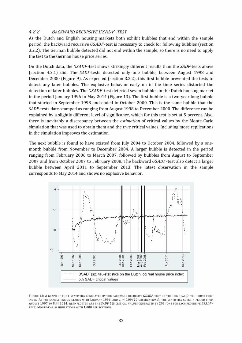
32

4.2.2 BACKWARD RECURSIVE -TEST As the Dutch and English housing markets both exhibit bubbles that end within the sample

period, the backward recursive -test is necessary to check for following bubbles (section

3.2.2). The German bubble detected did not end within the sample, so there is no need to apply

the test to the German house price series.

On the Dutch data, the -test shows strikingly different results than the SADF-tests above

(section 4.2.1) did. The SADF-tests detected only one bubble, between August 1998 and

December 2000 (Figure 9). As expected (section 3.2.2), this first bubble prevented the tests to

detect any later bubbles. The explosive behavior early on in the time series distorted the

detection of later bubbles. The -test detected seven bubbles in the Dutch housing market

in the period January 1996 to May 2014 (Figure 13). The first bubble is a two-year long bubble

that started in September 1998 and ended in October 2000. This is the same bubble that the

SADF-tests date-stamped as ranging from August 1998 to December 2000. The difference can be

explained by a slightly different level of significance, which for this test is set at 5 percent. Also,

there is inevitably a discrepancy between the estimation of critical values by the Monte-Carlo

simulation that was used to obtain them and the true critical values. Including more replications

in the simulation improves the estimation.

The next bubble is found to have existed from July 2004 to October 2004, followed by a one-

month bubble from November to December 2004. A larger bubble is detected in the period

ranging from February 2006 to March 2007, followed by bubbles from August to September

2007 and from October 2007 to February 2008. The backward -test also detect a larger

bubble between April 2011 to September 2013. The latest observation in the sample

corresponds to May 2014 and shows no explosive behavior.

FIGURE 13: A GRAPH OF THE -STATISTICS GENERATED BY THE BACKWARD RECURSIVE -TEST ON THE LOG REAL DUTCH HOUSE PRICE

INDEX. AS THE SAMPLE PERIOD STARTS WITH JANUARY 1996, AND (20 OBSERVATIONS), THE STATISTICS COVER A PERIOD FROM

AUGUST 1997 TO MAY 2014. ALSO PLOTTED ARE THE 5% CRITICAL VALUES GENERATED BY 202 (ONE FOR EACH RECURSIVE –TEST) MONTE-CARLO SIMULATIONS WITH 1,000 REPLICATIONS.

-20

24

Jan

19

96

Se

p 1

99

7

Se

p 1

99

8

Oct 2

00

0

Jul 20

04

De

c 2

00

4

Fe

b 2

00

6

Mar

200

7A

ug 2

00

7

Fe

b 2

00

8

Ap

r 20

11

Se

p 2

01

3

BSADF(s2) tau-statistics on the Dutch log real house price index

5% SADF critical values

33

These results show that Francke (2010), who was criticized by Knibbe (2010, p. 107) for failing

to detect an ‘obvious’ bubble, was right after all: there was no housing market bubble in 2009

anymore. In comparison to the results found in this thesis, other papers and reports estimating

overvaluation and bubbles (section 2.1) are very imprecise. For example, the IMF may have been

right to assert that a 30 percent gap between actual and fundamental house prices cumulated

between 1997 and 2007 (2008, p. 113). However, Figure 13 shows that any overvaluation in

that period is due to one large bubble between September 1998 and October 2000 and several

smaller bubbles between July 2004 and February 2008.

The bubble that existed between April 2011 and September 2013 is not or rarely mentioned in

other research. Its emergence is surprising, as had dropped since 2008 while the Dutch economy

was not performing very well. As there is no house price bubble at this moment (the last

observation is from May 2014), there should be no reason to expect a future decline of house

prices as the OECD (2014, p. 11) does.

Figure 14 shows the results of the backward -test on the English house price series. The

test found only one large bubble that existed from June 2006 to January 2008 and was followed

by a one-month bubble from February to March 2008. These results are almost the same as

those of the SADF-tests (Figure 12). In addition, at the end of the sample the -statistics seem to

be increasing. For a lower level of significance, May 2014 may even be the start of a new bubble.

Of course, no conclusions on the English housing market can or may be inferred from this

observation. Nevertheless, it is an encouragement to run new tests as more data on that market

becomes available.

FIGURE 14: A GRAPH OF THE -STATISTICS GENERATED BY THE BACKWARD RECURSIVE -TEST ON THE LOG REAL ENGLISH HOUSE PRICE

INDEX. AS THE SAMPLE PERIOD STARTS WITH JANUARY 2005, AND 13 (15 OBSERVATIONS), THE STATISTICS COVER A PERIOD FROM

MARCH 2006 TO MAY 2014. ALSO PLOTTED ARE THE 5% CRITICAL VALUES GENERATED BY 99 (ONE FOR EACH RECURSIVE –TEST) MONTE-CARLO SIMULATIONS WITH 1,000 REPLICATIONS.

The results found here are partly in line with the findings of Fry (2009) and Dreger and

Kholodilin (2013, p. 13) and show a bubble that ended in January 2008. However, Fry (2009),

-2-1

01

23

Ja

n 2

00

5

Ma

r 2

00

6

Ju

ne

20

06

Ja

n 2

00

8M

ar

20

08

Ma

y 2

01

4

BSAFD(s2) tau-statistics on the English log real house price index

5% SADF critical values

34

Dreger, and Kholodilin (2013, p. 13) asserted this bubble started in 2002. That is clearly not the

case, though a bubble might have existed before March 2006. Again, the method used in this

thesis is shown to generate much more precise results.

The IMF (2014, p. 26) and the Governer of the Bank of England (Treasury Committee, 2014)

warned about a possible house price drop. The results found here do not show a bubble, and

therefore, there is no reason to expect a burst. However, because of their respective roles as

policy advisors or makers, it may be prudent to rather risk ‘sounding the alarm’ too soon than

too late or not at all (section 3.2.2). As mentioned above, at a lower level of significance, a bubble

would perhaps have already been in May 2014.

The - and backward -tests have detected and pinpointed multiple bubbles in

housing markets, and research question 2 (section 2.7) has been satisfied.

4.3 REAL-TIME MONITORING The date-stamping procedure performed above is conceptually suited as a real-time monitoring

system (section 3.3). However, the -test cannot be used to detect new bubbles if there

already are bubbles in the sample used. The fact that the -test did not detect any Dutch

housing bubbles after 2000 (Figure 9) while we now know they were there (Figure 13) attests to

this assertion. One way around this problem is to apply the test only to the observations that

(chronologically) come after the end of the last bubble. There are two possible objections to this

approach. First, if a bubble just ended, it will take a while until a sufficiently large number of new

observations is available to resume monitoring the market. Second, this method disregards a lot

of data preceding the end of the last bubble that could contribute to the reliability of the

monitoring. Therefore, I recommend only using the -test for real-time monitoring if such a

test has already established that the market is bubble-free for a longer period of time.

The backward -test is not hindered by old bubbles to detect new ones (section 3.2.2).

Therefore, it is clearly the superior instrument in detecting new bubbles forming. It would most

likely have detected the Dutch housing bubble from 2011 to 2013 at its start, even though the

bubble is preceded by several others. As the English housing market visually (Figure 14) seems

to head for a new bubble, I would advise anyone with a substantial stake in that market

(including policy makers) to carefully monitor what happens in the next months. In order to do

this, they would have to add one observation to the sample each month, run the tests, and

generate additional critical values.

The results of this monitoring should be interpreted carefully due to the limitations of the

research methods used in this study (section 5). Choosing a lower level of significance allows

one to detect bubbles sooner, but also increases the risk that a ‘bubble’ is falsely detected

(section 3.2.2). However, provided that the results are interpreted carefully and the level of

significance is adapted to the purpose of the test, the backward -test can be used to

detect new housing bubbles.7 In this way, the backward -test fills a gap as many older

bubble detection methods may not be used for real-time monitoring (e.g., ECM, variance bounds

tests). Therefore, it should become part of the instruments of policy makers.

7 Of course, the backward -test can be applied to monitor other markets as well, such as stock markets and commodity markets.

35

Detecting emerging bubbles early, is of great importance. Bubbles tend to collapse eventually

and a collapse could lead to a sharp drop in housing prices, the results of which are discussed in

section 2.2. If a bubble is detected early, governments have more time to implement measures to

limit the negative impact a bubble may have. Governments could lower the maximum LTV (loan-

to-value ratio) allowed for mortgage loans so that banks and mortgagors are less exposed to the

risk that property value suddenly declines. The maximum DTI (debt-to-income ratio) allowed

can also be restricted for mortgage loans in order to limit the risk that borrowers will default on

them. That becomes more important for lenders (i.e., banks) as a negative house price shift

reduces the value of the collateral securing the loans. In fact, the IMF (2014, p. 7) recently

advised that German authorities they could use ‘LTV- and DTI-requirements to tackle possibly

emerging risks in the German housing markets.’

As real-time monitoring with the -test can be an early warning system for both the start

and ending of a bubble, research question 3 is answered affirmatively (section 2.7).

Furthermore, section 4.2 already showed the results of using this method on the most recent

data of each housing market. It established that there is no Dutch and no English housing bubble.

From the third quarter of 2012, however, there is a German housing bubble. Research question 4

is now also answered.

36

5. DISCUSSION This thesis produces some powerful results. It detected and date-stamped several housing

market bubbles. Because of the large impact of housing bubbles on home-owners and on

national economies (section 2.2), and because of the strong claims to date-stamping precision

this thesis’ method makes (section 3.2.2), careful interpretation of the results is necessary. This

section will therefore highlight some limits to the theoretical framework and the empirical

methodology that produced these results.

The elephant in the room when discussing the interpretation of this study’s results, is that the

rational bubble theory used in this study, assumes the strong-form Efficient Market Hypothesis

(EMH) for housing markets (A-II, section 2.5.1), while in fact market agents may not all have the

same information and may not have rational expectations. Even if one would concede to holding

the EMH as true, actual ex post rental income may not be appropriate to represent expected

rents. Theoretically, house prices at time could increase explosively in rational anticipation

(based on the information at that time, ) of an explosive rise of rent (Equation 6). If actual rents

do not follow expectations, the empirical methods used in this thesis will now find a bubble were

there was none. The ‘bubble’ was in fact an explosive increase in actual and fundamental prices

due to ‘wrong’ expectations. Siegel (Siegel, 2003, p. 17) asserts that even the famous Wall Street

crash of 1929 was not the collapse of a bubble as the 1920s bull market was justified by

expectations of higher dividends that eventually came true in the 1940s. Such claims can only be

refuted by using actual data on agents’ expectations, which – needless to say – is not available for

the markets investigated in this thesis.

House prices are influenced by more variables than only the (expected) rent. As discussed in

section 2.4, they are also affected by interest rates, demographics, and construction costs. To

account for these influences, Equation 14 incorporates them into the model by adding a variable

to represent the unobserved fundamentals. As explosive price behavior cannot be caused by

stationary fundamentals, the adding of this variable does not influence bubble detection as long

as the unobserved fundamentals do not behave explosively. For some fundamentals like

demographics and interest, it is conceptually hard to imagine explosive behavior as that would

signify a self-reinforcing process. As interest is largely determined by central banks, they would

have to let it behave explosively on purpose. Furthermore, other fundamentals often affect rent

and house prices symmetrically (section 2.4.3) (Brunnermeier & Julliard, 2006, p. 9). In that

case, those fundamentals would not undermine bubble detection even if they did behave

explosively.

The results found give insight on three national housing markets. These markets may not be the

appropriate markets to investigate for some purposes. Financial literature investigating bubbles

on stock markets often actually looks at composite indices (e.g., S&P 500, AEX, DAX, FTSE), and

therefore risks overlooking bubbles in specific stocks. In the same way, the tests performed in

this thesis that did not detect national housing bubbles in a certain period, do not exclude

regional bubbles in the same timeframe. London, for example, may have already gone through

its own housing bubble around 1990 (Case & Shiller, 2003, p. 302) and recently news media

started speaking of a London property bubble again.8 Even though this thesis establishes that

8 E.g.; New Statesman on April 3, 2014, Bloomberg Businessweek on May 22, 2014, and the London Evening Standard on March 28, 2014. Articles are retrieved at September 14, 2014 from these respective websites:

37

the last bubble on the English housing market ended in March 2008 (section 4.2.2), it is possible

that there actually is a London housing bubble at this moment. As discussed above in section

2.1.2, the Bundesbank (2013) did not think there was a bubble in the German housing market as

a whole. At the same time, however, it points at the possibility that house prices in seven major

German cities are overvalued.9 The Bundesbank also stresses that price movements may differ

between types of dwellings and distinguishes between apartments and (regular) houses. It

would be interesting to investigate whether aggregate figures actually hide local bubbles. The

search for local bubbles is very relevant to local governments, who often rely on local house

prices for income via property tax (section 2.2). As houses provide collateral for mortgage loans,

banks should also be interested in local bubbles, especially banks that are not geographically

diversified. There is, however, little data on regional housing markets. In light of the importance

to differentiate between a regional bubble and a larger (national) bubble, and new bubble

detection possibilities offered by the techniques used in this thesis, I would urge governments

(and others) to gather more geographically specified data on housing markets.

The empirical method used in this thesis claims to precisely date-stamp the start and ending of

bubbles. This claim needs to be relaxed somewhat. The dates found depend heavily on the level

of significance chosen for determining when there is explosive behavior. For example, Figure 13

shows -statistics and 5-percent critical values. If a line representing 1-percent critical values, it

would lie above the 5-percent critical values. Using these critical values, bubbles would be

determined to start later and end earlier. Some bubbles, like the bubbles between July 2004 and

December 2004, would probably not have been detected. Conversely, if a series of 10-percent

critical values was used, more bubbles might have been found. As discussed in section 3.2.2, the

significance level chosen should be adapted to the purpose of the test. Furthermore, according to

the rational bubble theory, the end of explosive behavior is equal to the end of all overvaluation

(section 3.2.1). In other words, a bubble’s crash is always immediate and there can be no soft

landings. Especially in markets like housing markets, with heterogeneous goods and low trading

frequencies (as opposed to stock markets), this corollary of the theory may not be realistic.

Developing and testing theory that allows for a slower return to fundamental value is a relevant

subject for future research and could contribute to a more accurate estimation of housing

bubbles’ end dates.

The data on Dutch rental income includes only yearly observations, instead of quarterly or

monthly observations. Many research on housing market bubbles uses yearly data, and rents are

not expected to be volatile in the short run, as levels of rent are often laid down in contracts to

be constant or to increase annually with (an indicator for) inflation. Nevertheless, because in this

thesis behavior from one period to the next is investigated, more frequent data could have

established the absence of explosive behavior in Dutch rents more accurately and, therefore,

more reliably.

http://www.newstatesman.com/politics/2014/04/five-signs-london-property-bubble-reaching-unsustainable-proportions http://www.businessweek.com/articles/2014-05-22/london-housing-market-may-be-in-bubble-territory http://www.standard.co.uk/news/london/london-living-through-biggest-house-price-bubble-ever-9221297.html. 9 These cities are Berlin, Hamburg, Munich, Cologne, Frankfurt am Main, Stuttgart, and Düsseldorf (Bundesbank, 2013, p. 15).

38

Real-time monitoring can detect the formation and the deflation of a bubble as it is happening.

Depending on the properties of the bubble component that bubble will collapse sooner or later.10

It is important to note, however, that the real-time monitoring procedure investigated and

subsequently advised in this study, does not predict when an existing bubble will end or when a

new bubble forms. Developing a model that actually predicts the collapse of housing market

bubbles would be an interesting and relevant subject for future research.

10 Equation A.1 and Equation A.2 describe possible bubble forms.

39

6. CONCLUSION Using different methods of recursive Augmented Dickey-Fuller tests, this thesis successfully

detected and date-stamped bubbles on the Dutch, German, and English housing market. On each

of these markets, the results have different implications.

The Dutch results show eight house price bubbles between January 1996 and May 2014. The

bubbles found are for a large part in line with existing research, though this thesis may add some

precision about when the bubbles started and collapsed. One surprising find is that a bubble

existed between April 2011 and September 2013, in spite of a weak economy. How and why this

bubble occurred is outside the scope of this thesis, but is an interesting topic for future research.

As expected, the German housing market did not exhibit bubbles for the most part of its sample

period (2000Q1 to 2013Q3). However, opposite to what some economists, the IMF and the OECD

assert, there is a bubble in the German housing market that started in 2012Q3.

This thesis also assessed the English housing market from January 2005 to May 2014. Somewhat

unsurprisingly, this thesis also found a bubble in that market: from June 2006 to January 2008.

More remarkable is that there has not been a bubble since. However, house prices are rising

steeply and the test statistic corresponding to May 2014 seems to approach the critical values

series (and would perhaps have been the start of a bubble at a lower level of significance). The

IMF has rightly warned the UK authorities to monitor developments in the near future.

In many countries, the application of this thesis’ method is impossible, because they lack

accurate data on house prices and (especially) rental income. In light of the importance of

knowing when housing bubbles exist and the possibilities offered by the methods described

here, every (developed) country should collect and provide this data. As the methods look at

time series behavior from one period to the next instead of directly looking at relationships

between variable levels, frequent data is very important and policy makers should ensure that

there are monthly observations on house prices rent.

The results generated in this thesis are much more precise than earlier research on these

respective markets and the -test and the backward -test are important instruments

to detect bubbles as they arise. They offer policy makers the opportunity to take measures in

preventing or contain costly housing bubbles. Therefore, these tests should be a part of policy

makers’ toolboxes.

40

BIBLIOGRAPHY Ambrose, B., Eichholtz, P., & Lindenthal, T. (2013). House Prices and Fundamentals: 355 Years of

Evidence. Journal of Money, Credit and Banking, 45, 477-491.

André, C. (2010). A Bird's Eye View of OECD Housing Markets. OECD Economics Department

Working Paper No. 746.

Baker, D. (2002). The Run-up in Home Prices: Is It Real or Is It Another Bubble? Briefing Paper,

Centre for Economic and Policy Research.

Baker, D. (2008). The Housing Bubble and the Financial Crisis. Real-world economics review, 73-

81.

Blanchard, O., & Watson, M. (1982). Bubbles, Rational Expectations and Financial Markets. NBER

Working Paper No. 945.

Brancaccio, E. (2005). Stock Markets and Bubbles. Quaderno DASES, 7, 25-37.

Brunnermeier, M., & Julliard, C. (2006). Money Illusion and Housing Frenzies. NBER Working

Paper No. 12810.

Bundesbank. (2013). Monthly Report October 2013.

Campbell, J., Lo, A., & MacKinlay, A. (1997). The Econometrics of Financial Markets. Princeton

University Press.

Case, K., & Shiller, R. (1989). The Efficiency of the Market for Single-Family Homes. American

Economic Review, 79(1), 125-137.

Case, K., & Shiller, R. (2003). Is There a Bubble in the Housing Market. Brookings Paper on

Economic Activity, 2, 299-362.

Case, K., Shiller, R., & Quigley, J. (2005). Comparing Wealth Effects: The Stock Market Versus the

Housing Market. Advances in Macroeconomics, 5(1).

Chan, H., Lee, S., & Woo, K. (2001). Detecting rational bubbles in the residential housing market

of Hong Kong. Economic Modelling, 18, 61-73.

Chen, X., & Funke, M. (2013). Renewed Momentum in the German Housing Market: Boom or

Bubble? CESifo Working Paper No. 4287.

Chu, C.-S., Stinchcombe, M., & White, H. (1996). Monitoring Structural Change. Econometrica,

64(5), 1045-1065.

CPB. (2005). Welke factoren bepalen de ontwikkelingen van de huizenprijs in Nederland? CPB

Document No. 81.

CPB. (2008). Are houses overvalued in the Netherlands? CPB Memorandom No. 200.

Diba, B., & Grossman, H. (1988a). Explosive rational bubbles in stock prices? American Economic

Review, 78, 520-530.

41

Diba, B., & Grossman, H. (1988b). The theory of rational bubbles in stock prices. The Economic

Journal, 98, 746-754.

Dreger, C., & Kholodilin, K. (2013). An Early Warning System to Predict Speculative House Price

Bubbles. Economics: The Open-Access, Open-Assessment E-Journal, 7.

Engsted, T., & Nielsen, B. (2012). Testing for rational bubbles in a coexplosive vector

autoregression. The Econometrics Journal.

Evans, G. (1991). Pitfalls in testing for explosive bubbles in asset prices. American Economic

Review, 31, 922-930.

Feld, L., Schulten, A., Jahn, M., Simons, H., & Kiefer, M. (2014). Frühjahrsgutachten

Immobilienwirtschaft 2014 des Rates der Immobilienweisen, Zusammenfassung. Retrieved

April 29, 2014, from Zentraler Immobilien Ausschuss: http://www.zia-

deutschland.de/presse/pressemitteilungen/rat-der-immobilienweisen-trotz-

gestiegener-preise-keine-blase/, retrieved at April 29, 2014.

Francke, M. (2010). Casametrics. The art of modeling and forecasting the market value of houses.

Inaugural lecture, Amsterdam.

Francke, M., Vujić, S., & Vos, G. (2009). Evaluation of house price models using an ECM approach:

The case of the Netherlands. Working Paper. ORTEC Finance Research Center.

Friedman, M. (1966). The Methodology of Positive Economics. Essays in Positive Economics, pp.

3-16, 30-43.

Fry, J. (2009). Bubbles and contagion in English house prices. MPRA Paper No. 17687.

Gallin, J. (2003). The Long-Run Relationship between House Prices and Income: Evidence from

Local Housing Markets. Finance and Economics Discussion Series No. 2003-17.

Gallin, J. (2004). The Long-Run Relationship between House Prices and Rents. Finance and

Economics Discussion Series No. 2004-50.

Geltner, D., Miller, N., Clayton, J., & Eichholtz, P. (2007). Commercial Real Estate Analysis and

Investments. Mason, Ohio: Cengage Learning.

Girouard, N., Kennedy, M., Noord, v. d., & André, C. (2006). Recent House Price Developments:

The Role of Fundamentals. OECD Economics Department Working Papers No. 475.

Glaeser, E., & Gyourko, J. (2007). Arbitrage in Housing Markets. NBER Working Paper Series No.

13704.

Gürkaynak, R. (2008). Econometric Tests of Asset Price Bubbles: Taking Stock. Journal of

Economic Surveys, 22(1), 166-186.

Hall, R. (2001). Struggling to Understand the Stock Market. American Economic Review, 91(2), 1-

11.

Hamilton, J., & Whiteman, C. (1985). The Observable Implications of Self-fulfilling Expectations.

Journal of Monetary Economics, 16, 353-373.

42

Heyer, E., Le Bayon, S., Péléraux, H., & Timbeau, X. (2005). L'immobilier, pilier de la croissance ou

épée de Damoclès. Bulle immobilière, causes et conséquences macro-économiques d’un

retournement du marché immobilier. Document de travail de l'OFCE No. 2005-16.

Hill, R., Griffiths, W., & Lim, G. (2011). Principles of Econometrics (4th ed.). New York: John Wiley

& Sons.

Homm, U., & Breitung, J. (2012). Testing for Speculative Bubbles in Stock Markets: A Comparison

of Alternative Methods. Journal of Financial Econometrics, 10(1), 198-231.

Hwang-Smith, M., & Smith, G. (2006). Bubble, Bubble, Where's the Housing Bubble? Brookings

Papers on Economic Activity, 1.

International Monetary Fund. (2008). Housing and the Business Cycle. IMF World Economic

Outlook April 2008.

International Monetary Fund. (2009). Staff Report. Kingdom of the Netherlands - Netherlands:

2009 Article IV Consultation.

International Monetary Fund. (2011). Statement by the Executive Director. Kingdom of the

Netherlands - Netherlands: 2011 Article IV Consultation.

International Monetary Fund. (2014). Staff report. United Kingdom: 2014 Article IV Consultation.

International Monetary Fund. (2014). Staff report. Germany: 2014 Article IV Consultation.

Just, T., Möbert, J., & Heinrich, M. (2013). Deutsche Wohnimmobilien als Kapitalanlage. Retrieved

April 29, 2014, from International Real Estate Business School, Universität Regensburg:

http://publications.irebs.de/immobilien

wirtschaft/6_IREBS_Deutsche_Wohnimmobilien_als_Kapitalanlage.pdf

Kindleberger, C., & Aliber, R. (2005). Manias, panics and crashes: a history of financial crises. New

York: John Wiley & Sons.

Kivedal, B. (2012). Testing for rational bubbles in the housing market. Working Paper Series

13312, Department of Economics, Norwegian University of Science and Technology.

Knibbe, M. (2010). Why did Dutch economists get it so wrong? Real-world Economics Review, 54,

106-119.

Kofner, S. (2014). The German housing system: fundamentally resilient? Journal of Housing and

the Built Environment, 29, 255-275.

Komáromi, G. (2006). The Anatomy of Stock Market Bubbles. The ICFAI University Press.

Kuenzel, R., & Bjørnbak, B. (2008). The UK Housing Market: Anatomy of a house price boom.

Economic Analysis from the European Commission's Directorate-General for Economic and

Financial affairs, 5(11).

LeRoy, S. (2004). Rational Exuberance. Journal of Economic Literature, 42(3), 783-804.

43

LeRoy, S., & Porter, R. (1981). The present-value relation: tests based on implied variance

bounds. Econometrica, 49, 555-574.

Lind, H. (2009). Price Bubbles on the Housing Market: Concept, theory and indicators.

International Journal of Housing Markets and Analysis, 2(1), 78-90.

McQuinn, K., & O'Reilly, G. (2008). Assessing the role of income and interest rates in determining

housing prices. Economic Modelling, 25, 377-390.

Minsky, H. (1972). Financial Instability Revisited: The Economics of Disaster. Reappraisal of the

Federal Reserve Discount Mechanism.

OECD. (2005). Recent House Price Developments: The Role of Fundamentals. OECD Economic

Outlook 78, 123-154.

OECD. (2014). OECD Economic Surveys: Germany.

OECD. (2014). OECD Economic Surveys: Netherlands .

Phillips, P., Shi, S., & Yu, J. (2012). Testing for Multiple Bubbles. Discussion Paper no. 1843, Cowles

Foundation for Research in Economics, Yale University.

Phillips, P., Wu, J., & Yu, J. (2011). Explosive Behavior in the 1990s Nasdaq: When Did

Exuberance Escalate Asset Values? International Economic Review, 52(1), 201-226.

Reinhart, C., & Rogoff, K. (2008). Is the 2007 US Sup-prime Financial Crisis so different? An

International Historical Comparison. The American Economic Review, 52(1), 339-344.

Shi, S. (2007). Moving Window Unit Root Test: Locating Real Estate Price Bubbles in Seoul

Apartment Market. Retrieved April 27, 2014, from Institutional Knowledge at Singapore

Management University: http://ink.library.smu.edu.sg/etd_coll/28

Shiller, R. (1981). Do Stock Prices Move Too Much to be Justified by Subsequent Changes in

Dividends? American Economic Review, 71, 421-436.

Shiller, R. (2005). Irrational Exuberance. Princeton University Press.

Shiller, R. (2007). Understanding Recent Trends in House Prices and Home Ownership. Cowles

Foundation Discussion Paper No. 1630, Yale University.

Siegel, J. (2003). What Is an Asset Price Bubble? An Operational Definition. European Financial

Management, 9(1), 11-24.

Stiglitz, J. (1990). Symposium on bubbles. The Journal of Economic Perspectives, 4(2), 13-18.

Treasury Committee, H. o. (2014, July 15). Oral evidence: Bank of England June 2014 Financial

Stability Report. Retrieved September 11, 2014, from

http://data.parliament.uk/writtenevidence/committeeevidence.svc/evidencedocument

/treasury-committee/bank-of-england-financial-stability-reports/oral/11464.html

44

Tschekassin, O. (2014). The myth of a new housing bubble in Germany. Retrieved September 11,

2014, from Bruegel (blog): http://www.bruegel.org/nc/blog/detail/article/1359-the-

myth-of-a-new-housing-bubble-in-germany/

Van der Wal, E., & Tamminga, W. (2008). Why the average dwelling purchase price is not an

indicator. Retrieved April 29, 2014, from Statistics Netherlands:

http://www.cbs.nl/NR/rdonlyres/CBCED024-0236-40EE-AD8A-

6ECCC7A139C7/0/Whytheaveragedwellingpurchasepriceisnotanindicator.pdf

Yiu, M., & Lu, Y. (2012). Detecting Bubbles in the Hong Kong Residential Property Market: An

Explosive-Pattern Approach. HKIMR Working Paper No. 01/2012.

45

APPENDIX A: BUBBLE FORMS As section 2.5.2 mentioned, the bubble component that contributes to the actual price of an asset

(Equation 10) can have several theoretical properties. This appendix describes and discusses

two bubble forms suggested in literature.

Blanchard and Watson suggest a bubble of the following form (Homm & Breitung, 2012, p. 201):

Equation A.1 {.

/

As ( ) , Equation A.1 obeys Equation 11. As long as the bubble does not burst, it grows

at a rate .

/ , which is faster than , thereby compensating for the probability of bursting.

There is a theoretical problem with this time of bubble model. Diba & Grossman (1988b, p. 751)

argue that a bubble cannot start from zero, so any bubble that exists must have been there since

the first moment the asset was traded. Furthermore, when a bubble has collapsed, it can never

restart. The reasoning goes as follows. As explained above, a negative bubble defies rationality

and therefore cannot exist within a rational bubble model. When the bubble has a zero value,

the expected bubble value in the future is also zero according to Equation 11 and Equation A.1.

Since a bubble cannot be negative, the expected bubble value can only be zero, if there is also no

chance the actual bubble component will be positive. In other words, a zero value bubble must

be expected to remain at zero value, and it can only have a zero expectation if it is zero in the

future with probability one, see also Campbell et al. (1997, p. 259).

Though no-one has been able to fully address the Diba & Grossman (1988b) critique, other

suggested bubble models have mitigated the problem. Evans (1991) proposes a periodically

collapsing bubble model that has an initial bubble value :

Equation A.2 {( )

, ( ) ( ( ) )-

Here, is an independently and identically distributed random variable that is exogenous to

the model, with and ( ) . and are parameters with ( ) and

., and is an exogenous independently and identically distributed Bernoulli process for

which goes that with probability and with probability , where .

This bubble model also satisfies Equation 11. As long as , the bubble grows at a rate of

( ) and is expected to grow at a rate of . This process continues until a limit of is

reached. Thereafter, when , the existing bubble starts to inflate more rapidly at an

expected rate of ( ) until it collapses when and the bubble starts growing again at

expected rate of . As with the bubble process proposed by Blanchard & Watson (1982)

explained above, if is smaller, the bubble will grow faster during its ‘inflationary phase’. This

effect is offset by the fact that the probability of a bubble deflating is and therefore faster

growth rate means a higher probability of collapse. After the bubble’s collapse, the bubble

component reverts to , where , so Evans’ (1991) bubble model is a solution to the

Diba & Grossman (1988b) critique that bubbles cannot restart once deflated. It still needs to

assume, however, that there is a bubble initially.

46

APPENDIX B: TIME SERIES’ GRAPHS

FIGURE B.1: THE DUTCH LOGARITHMIC REAL HOUSE PRICE INDEX, CONTAINING 221 MONTHLY OBSERVATIONS. VISUALLY, THE SERIES SEEMS

TO FIT THE MODEL WITH A CONSTANT AND NO TREND: .

FIGURE B.2: THE DUTCH LOGARITHMIC REAL RENTAL INCOME INDEX, CONTAINING 18 ANNUAL OBSERVATIONS. VISUALLY, THE SERIES SEEMS

TO FIT THE MODEL WITH A CONSTANT AND A TREND: .

3.8

44

.24

.44

.6

Dutc

h lo

g r

ea

l ho

use

price

ind

ex

1995m1 2000m1 2005m1 2010m1 2015m1

47

FIGURE B.3: THE GERMAN LOGARITHMIC REAL HOUSE PRICE INDEX, CONTAINING 55 QUARTERLY OBSERVATIONS. VISUALLY, THE SERIES SEEMS

TO FIT THE MODEL WITH A CONSTANT AND A TREND: .

FIGURE B.4: THE GERMAN LOGARITHMIC REAL RENTAL INCOME INDEX, CONTAINING 165 MONTHLY OBSERVATIONS. VISUALLY, THE SERIES

SEEMS TO FIT THE MODEL WITH A CONSTANT AND A TREND: .

4.6

4.6

54

.74

.75

4.8

Germ

an lo

g r

ea

l ho

use

price

ind

ex

2000q1 2003q3 2007q1 2010q3 2014q1

48

FIGURE B.5: THE ENGLISH LOGARITHMIC REAL HOUSE PRICE INDEX, CONTAINING 113 MONTHLY OBSERVATIONS. VISUALLY, THE SERIES SEEMS

TO FIT THE MODEL WITH A CONSTANT AND NO TREND:

FIGURE B.6: THE ENGLISH LOGARITHMIC REAL RENTAL INCOME INDEX, CONTAINING 113 MONTHLY OBSERVATIONS. VISUALLY, THE SERIES

SEEMS TO FIT THE MODEL WITH A CONSTANT AND A TREND: .

4.9

5

5

5.0

55

.15

.15

En

glis

h log

re

al h

ou

se p

rice in

de

x

2005m1 2010m1 2015m1

4.4

4.4

54

.54

.55

4.6

En

glis

h log

re

al re

nta

l in

co

me in

de

x

2005m1 2010m1 2015m1