Fixational Eye movements in

Strabismic amblyopia

by

Rajkumar Nallour Raveendran

A thesis

presented to the University of Waterloo

in fulfillment of the

thesis requirement for the degree of

Master of Science

in

Vision Science

Waterloo, Ontario, Canada, 2013

©Rajkumar Nallour Raveendran 2013

ii

AUTHOR'S DECLARATION

I hereby declare that I am the sole author of this thesis. This is a true copy of the thesis, including any

required final revisions, as accepted by my examiners.

I understand that my thesis may be made electronically available to the public.

iii

Abstract

Purpose: To test the hypothesis that the fixational stability (FS) of the amblyopic eye (AME) in

strabismics will improve when binocular integration is enhanced through ocular alignment and inter-

ocular suppression is attenuated by reducing the contrast to the fellow eye (FFE).

Methods: 7 strabismic amblyopes (age: 30.8±9.7 yrs) (5 esotropes and 2 exotrope) (VA:

AME=0.50±0.30; FFE=-0.12±0.04) showing clinical characteristics of central suppression were

recruited. Suppression was then attenuated by a balance point procedure where the contrast to the

FFE was reduced in order to maximize binocular integration during a global motion task (GMT)

(Baker, 2007). In one case the balance point could not be determined, and the participant was

excluded. Ocular alignment was established with a haploscope. Participants dichoptically viewed

similar targets [a cross (2.3°) surrounded by a square (11.3°) visual angle] set at 40cm. Target

contrasts presented to each eye were either equal (EQ) or attenuated in the FFE (UNEQ) by an

amount defined by the GMT. FS was measured over a 5 min period (Viewpoint® Eye Tracker,

Arrington Research) and quantified using bivariate contour ellipse areas (BCEA) in four different

binocular conditions; unaligned/EQ, unaligned/UNEQ, aligned/EQ and aligned/UNEQ. FS was also

measured in 6 control subjects (Age: 25.3±4 yrs; VA: -0.1±0.08).

Results: Alignment of the AME was transient and lasting between 30 to 80 seconds. Accordingly, FS

was analyzed over the first 30 seconds using repeated measures ANOVA. Post hoc analysis revealed

that for the amblyopic subjects, the FS of the AME was significantly improved in aligned/EQ

(p=0.015) and aligned/UNEQ (p=0.001). FS of FFE was not different statistically across conditions.

BCEAFFE & BCEAAME were then averaged for each amblyope in the 4 conditions and compared with

normals. This averaged BCEA (reduced FS) was significantly greater (p=0.0205) in amblyopes

compared to controls except in the case of alignment coupled with reduced suppression

(aligned/UNEQ) (p=0.1232).

iv

Conclusion: Fixation stability in the amblyopic eye of strabismics appears to improve directly with

the degree of binocular integration. The hypothesis is therefore retained.

v

Acknowledgements

I would like to express my deep gratitude to my supervisor Dr. William R Bobier for his

guidance and valuable suggestions which helped me to complete this thesis work

successfully.

I would like to thank my committee members Dr. Vasudevan Lakshminarayan, Dr.

Robert F Hess and Dr. Raiju Babu for their valuable comments and suggestions.

I would like to thank my all study participants.

I would like to sincerely acknowledge all the members of Bobier’s Lab; Dr. Raiju Babu

for his immediate guidance and help throughout this thesis work. Dr. Vidhyapriya

Sreenivasan, Peng Zhang, Vivek Labhishetty and Nicholas Lorentz for offering help

whenever needed.

I would like to appreciate the help offered by Dr. Ziawei Zhou, McGill University, for

writing MATLAB code.

Thanks to Andrew Nowinski for his technical support. Jim Davidson and Chris Mathers

for computing support.

I would also like to thank Graduate Officers Dr. Trefford Simpson, Dr. Vivian Choh and

Dr. Natalie Hutchings for their help and the Graduate coordinator Krista Parsons for her

help.

Finally, I thank all my fellow grad students (GIVS), staffs and faculties of the School of

Optometry for making this pleasant working environment.

vi

Dedication

This thesis is dedicated to the

Almighty God

and

to my beloved family members

(My dad, mom, brother, sister-in-law and my niece Rakshanaa).

vii

Table of Contents

AUTHOR'S DECLARATION ............................................................................................................... ii

Abstract ................................................................................................................................................. iii

Acknowledgements ................................................................................................................................ v

Dedication ............................................................................................................................................. vi

Table of Contents ................................................................................................................................. vii

List of Figures ....................................................................................................................................... ix

List of Tables ......................................................................................................................................... xi

Chapter 1 REVIEW ON BINOCULAR VISION OF NORMALS AND STRABISMICS ................... 1

1.1 Binocular vision in normals: ........................................................................................................ 1

1.2 Binocular vision in strabismus: .................................................................................................... 4

1.2.1 Anomalous retinal correspondence (ARC): .......................................................................... 5

1.2.2 Suppression: .......................................................................................................................... 9

1.3 Amblyopia .................................................................................................................................. 13

1.3.1 Definition and types ............................................................................................................ 13

1.3.2 Amblyopia and Suppression ................................................................................................ 14

1.4 Binocular integration: ................................................................................................................. 15

Chapter 2 : FIXATION EYE MOVEMENTS IN NORMALS AND AMBLYOPES ......................... 20

2.1 Introduction ................................................................................................................................ 20

2.1.1 Fixation in normals: ............................................................................................................. 20

2.1.2 Fixation eye movements in amblyopes: .............................................................................. 22

Chapter 3 : OBJECTIVE OF THE STUDY ......................................................................................... 25

Chapter 4 : INSTRUMENTATION AND METHOD ......................................................................... 26

4.1 Ocular Alignment ....................................................................................................................... 26

4.1.1 Calibration of the haploscope .............................................................................................. 28

4.2 Attenuating inter-ocular suppression: ......................................................................................... 30

4.2.1 Description of the stimuli: ................................................................................................... 31

4.2.2 Reducing contrast of the stimulus to the fellow fixing (normal) eye: ................................. 31

4.3 Measuring eye movements: ........................................................................................................ 32

4.3.1 Setting up Eyetracker to measure eye movements: ............................................................. 33

4.3.2 Calibration of the eye tracker: ............................................................................................. 34

4.4 Participant selection: .................................................................................................................. 36

viii

Chapter 5 : RESULTS ......................................................................................................................... 42

5.1 Qualitative analysis of fixation pattern: ..................................................................................... 42

5.1.1 Fixation pattern in normals: ................................................................................................ 42

5.1.2 Fixation patterns in strabismic amblyopes: ......................................................................... 43

5.2 Quantitative analysis of fixation stability: ................................................................................. 47

5.2.1 Standard deviation of Horizontal eye positions (fixation error): ........................................ 47

5.2.2 Bivariate Contour Ellipse Area (BCEA): ............................................................................ 49

5.3 Direction of drifts: ...................................................................................................................... 54

5.4 Correlation of horizontal eye position: ...................................................................................... 55

Chapter 6 : DISCUSSION ................................................................................................................... 56

6.1 Fixation stability in normal observers ........................................................................................ 57

6.2 Fixation stability in strabismic amblyopes ................................................................................. 58

6.3 Effect of aligning strabismus: .................................................................................................... 59

6.4 Effect of attenuating inter-ocular suppression on fixation stability: .......................................... 60

6.5 Binocular fixational stability: ..................................................................................................... 60

6.6 Restoring original deviation of strabismus ................................................................................ 61

6.7 Conjugacy of fixational eye movements: ................................................................................... 62

Appendix A Haploscope – Optical theory ........................................................................................... 66

Appendix B Gamma Correction .......................................................................................................... 68

Appendix C Calculation of Weber’s contrast ...................................................................................... 71

Copyright Permission ........................................................................................................................... 73

References ............................................................................................................................................ 79

ix

List of Figures

Figure 1-1: Crossed and uncrossed disparity. ......................................................................................... 3

Figure 1-2: Confusion and Diplopia ....................................................................................................... 4

Figure 1-3: Normal and Anomalous retinal correspondence .................................................................. 6

Figure 1-4 Different precieved response of Worth four dot test .......................................................... 13

Figure 1-5: Perceived responses from BSGT ....................................................................................... 13

Figure 1-6: Models of binocular vision ................................................................................................ 16

Figure 1-7: Random dot kinematograms (RDK). ................................................................................. 18

Figure 1-8: Balance point calculation. .................................................................................................. 18

Figure 4-1: Schematic and actual picture of the haploscopic setup ...................................................... 27

Figure 4-2: Empirical (measured eye rotation) values as a function of calculated values (actual eye

rotation) Error bars represent 1 SD. ..................................................................................................... 29

Figure 4-3: Dissimilar target used for the calibration of haploscope. .................................................. 29

Figure 4-4: Stimulus for fixational and vergence eye movments. ........................................................ 30

Figure 4-5: Eyetracker mounted on a spectacle frame. ........................................................................ 33

Figure 4-6: interface of software Viewpoint®. .................................................................................... 35

Figure 4-7: Stimulus for calibration of eye tracker. ............................................................................. 35

Figure 4-8: Four different viewing conditions used to measure fixational stability. ............................ 37

Figure 4-9: Target for the participants (normals and strabismics) to fixate with equal contrast to both

eyes. ...................................................................................................................................................... 39

Figure 4-10: Target for the strabismic participants to fixate with balanced (reduced) contrast to the

fellow eye ............................................................................................................................................. 39

Figure 5-1: Monocular viewing eye trace of normal participant .......................................................... 42

Figure 5-2: Binocular viewing eye trace of normal participant ............................................................ 42

Figure 5-3: Fixation eye trace of the participant XU. ........................................................................... 44

Figure 5-4: Fixation eye trace of the participant (OT) ......................................................................... 45

Figure 5-5: Initial 30 seconds vs. last 3 minutes .................................................................................. 46

Figure 5-6: Fixation error in the horizontal eye position of Normal observers. ................................... 47

Figure 5-7: Fixational error in the horizontal eye positions of strabismic amblyopes ......................... 48

Figure 5-8: BCEA of normal observers ................................................................................................ 49

Figure 5-9: BCEA of AME .................................................................................................................. 51

Figure 5-10: BCEA of FFE .................................................................................................................. 51

x

Figure 5-11: Binocular BCEA of strabismic amblyopes ..................................................................... 52

Figure 5-12: Strabismic amblyopes vs. Normal observers .................................................................. 53

Figure 5-13: Direction of drifts in the strabismic participant (XU), an esotrope ................................. 54

Figure 5-14: Direction of drifts in the strabismic participant (AD), an exotrope ................................ 54

Figure 6-1: Optical theory of haploscope ............................................................................................ 66

Figure 6-2: Gamma .............................................................................................................................. 70

xi

List of Tables

Table 4-1: Values of the calculated and the empirical values of eye rotation. ..................................... 29

Table 4-2: Specification of the eyetracker ............................................................................................ 32

Table 4-3: Details of sensory and motor status of the participants ....................................................... 41

Table 5-1: Period of initial optimal fixation ......................................................................................... 46

Table 5-2: Correlation coefficients of horizontal eye positions in strabismic amblyopes during

fixation.................................................................................................................................................. 55

Table 5-3: Correlation coefficients of horizontal eye positions in normals during fixation ................. 55

Table 6-1: Values of Luminance .......................................................................................................... 69

Table 6-2: Weber’s contrast ratio ......................................................................................................... 72

1

Chapter 1

REVIEW ON BINOCULAR VISION OF NORMALS AND STRABISMICS

1.1 Binocular vision in normals:

Imagine an object at a suitable distance in front in the mid plane of the head. If the

eyes are properly aligned and if the object is fixated binocularly then the image would fall on

corresponding retinal points. Thus the corresponding retinal points are the retinal

element/retinal point which when stimulated simultaneously will give rise to a single

binocular percept 21,26,47,56

. Each retinal element localizes the object in a specific direction

and it is relative to the fovea (the retinal area with highest visual acuity). Thus, the

corresponding retinal points can also be defined as the points that share the same visual

direction. In normal binocular vision, therefore, both foveas have same visual direction

(corresponding retinal points) and the phenomenon is called normal retinal correspondence

56.

The corresponding retinal points are distributed throughout the retina and locus of

these retinal points, in visual space, is called horopter. In other words, any point in the

horopter would stimulate corresponding retinal points. In visual space, this horopter forms an

arc of a circle called Vieth Muller Circle 21,56

. This is the ideal or theoretical horopter. It is a

circle which passes through nodal points of the eyes and the fixation point (figure: 1-2).

There is a small area in front and back of the horopter in which single vision is present is

called Panum’s fusional area. This area is about 0.5° around the horopter 47,48

. When eyes

are fixating on an object, there is always a minute variation in binocular vision which is

2

within Panum’s fusional area and this is called fixation disparity 33,40

. Panum’s fusional area

and fixation disparity are responsible for stereoscopic vision 56

.

In figure: 1-1, the visual axes are converged at the fixation point. The point A which

is nearer to the observer than the horopter produces crossed retinal disparity (crossed

images). This is called crossed disparity (images) because, with monocular viewing, midline

of the point A appears on the opposite side of the fixation point. This is also known as

convergent disparity. The point B is beyond the horopter and produces uncrossed disparity.

This is called uncrossed disparity because with monocular viewing, midline of the point B

appears on the same side to the fixation point. If these disparities lie outside the Panum’s

fusional area, they will induce motor fusion i.e. fusional vergence eye movements; crossed

disparity induces convergent eye movement whereas uncrossed disparity induces divergent

eye movement. Thus each retinal point has some retinomotor value. This retinomotor value

increases from the center towards the periphery. The fovea is called the retinomotor center or

retinomotor zero point because, once the image is on fovea, there is no need for any further

eye movement21,56

.

However, to perceive the images falling on the foveas and other corresponding retinal

points as a single percept, sensory fusion is required and it takes place in the visual

cortex21,47,56

. The term sensory fusion is defined as unification of excitations from

corresponding retinal images into single visual percept. In other words, the stimulus to

sensory fusion is excitation of corresponding retinal points 56

. For sensory fusion, images not

only must fall on corresponding retinal points but also must be in similar size, contour and

brightness46

. The simultaneous stimulation of non-corresponding retinal points by a similar

3

object induces double vision/diplopia. But the ability to align the eyes in such a manner (i.e.

move it in opposite direction – fusional vergence) to maintain the sensory fusion is termed as

motor fusion. Thus the retinal disparity is stimulus for motor fusion. For motor fusion, again

the images must be similar in size and fall outside the Panum’s area.

Figure 1-1: Crossed and uncrossed disparity.

Vieth Muller circle is the circle passing through point of fixation and the nodal points. The images of

point A are crossed because their visual lines cross inside the horopter. The images of point B are

uncrossed because their visual lines cross beyond the horopter [Image duplicated from Howard and

Rogers, 1995].

Binocular Rivalry:

When dissimilar contours are presented to corresponding retinal points, fusion is not

possible but a binocularly-based rivalry may be observed. In other words, such excitations

are localized in the same visual direction which results in conflict or confusion. Rivalry

could also be induced by uniform surface of different colors (color rivalry) and unequal

luminance of the two targets. Our visual system responds to such rivalries by suppressing one

A

Crossed images of point A

Vieth-Müller Circle

Fixation point Uncrossed images of point B

4

of the images. Which of the images is suppressed depends on the dominance of one eye

rather than the quality of images like contour, luminance or color 8,56

.

Figure 1-2: Confusion and Diplopia

a) explains the phenomenon of confusion where dissimilar images fall on corresponding retinal points

and, b) explains the phenomenon of diplopia where similar images stimulating non corresponding retinal

points (Image adapted from Von Noorden, 2002)

1.2 Binocular vision in strabismus:

The lack of alignment of the primary lines of sight with the object of regard in

strabismus leads to the object being imaged on the fovea of one eye and a non foveal point of

the turned eye. If normal correspondence is present, then it results in diplopia and confusion

(Figure: 1-2). The former arises due the image of the object of regard falling on non-

corresponding points whereas the latter due to differing images falling on the fovea.

However, if the strabismus is long standing then the visual system can invoke one of two

5

sensory adaptations which serve to reduce the diplopia and confusion: anomalous retinal

correspondence (ARC) or suppression. Small angle strabismics usually adapt to ARC

whereas large angle strabismics adapt to suppression 24

. Understanding of these adaptations

has been primarily based in clinical literatures 3,21,24,56

.

However, existence of such adaptations is really debatable. For instance, Schor (1991)

points out that it is remarkable that ARC as described could exist. In the case of infantile

esotropia where the strabismus has developed in early developmental ages, there would be

very little opportunity for the underpinning of correspondence between two eyes and the

development of binocular vision through anomalous correspondence.

1.2.1 Anomalous retinal correspondence (ARC):

ARC is defined as the perception of foveal stimuli in the two eyes in separate visual

directions. In other words, it describes a situation where apparently the correspondence of the

deviated eye is compromised such that the non-foveal point in the deviated eye is given the

same visual direction as that of the fovea of the fixing eye 56

. Thus diplopia and confusion are

avoided. The angle separating this corresponding point and the anatomical fovea of the

deviating eye is called angle of anomaly (A). If the angle of anomaly (A) equals the objective

angle of strabismus, then it is termed as Harmonious ARC (HARC). If the angle of anomaly

(A) did not equal the objective angle (H), then it is termed as Unharmomious ARC and the

retinal disparity equal to the difference (H-A) could stimulate diplopia. This difference in the

angle is called subjective angle of strabismus (S) 24,47,56

. ARC can be very variable and at

times it may co-exist with suppression. Clinical tests are always biased where the Bagolini

Striated glass test (description in the section 1.2.2.3) will show ARC more frequently than

6

Worth’s four dot test. As with suppression, ARC can be altered with changes in luminance

and contrast 6.

Figure 1-3: Normal and Anomalous retinal correspondence

A) After Image test showing Normal retinal correspondence where the foveas of the two eyes having same

visual direction and B) after image test showing abnormal retinal correspondence where the foveas of the

two eyes have different visual direction (adapted from Von Noorden, 2002).

1.2.1.1 Theories of ARC:

The main question is how does an elaborate system of ARC evolve where

correspondence can be adjusted with each position to keep both retinal images with same

visual direction? There are two schools of thought regarding ARC. One of these schools of

thought thinks that ARC is a sensory adaptation to avoid diplopia/confusion (ambiocular

vision) whereas the other thinks that ARC is a primitive form of vision (utrocular vision)

found normally in vertebrates with complete decussation of the visual pathways.

7

1.2.1.1.1 Utrocular vision:

Schor (1991) has pointed out the elegant theory of Walls (1951). Based upon his deep

understanding of comparative vision, it is postulated that what is called ARC could really

represent a regression to utrocular vision such as that experienced by a species that has no

binocular vision. In lower vertebrates, the visual cortical hemisphere receives inputs

completely from the contralateral eye and also they have laterally placed eyes which support

a form of panoramic vision. The visual directions of the two eyes are compared more

egocentrically (Egocentric visual direction refers to the visual direction of an object in space

relative to oneself, rather than the eyes). Schor (1991)47

has stated neurophysiological and

psychophysical correlates to substantiate that ARC is a form of utrocular form of vision.

1.2.1.1.2 Ambiocular vision:

The hypothesis of utrocular vision cannot be fully accepted as the subjects with ARC

do exhibit binocular functions like reduced stereopsis and vergence eye movements. So, the

other school of thought thinks that ARC is a sensory adaptation which has limited form of

binocular vision and compares visual direction more oculocentrically, rather egocentrically

as in utrocular vision. Correspondence shift and enlarged fusional area are the two

organization of binocular vision that substantiates ARC is an ambiocular vision.

Correspondence shift:

This is a classical theory of ARC suggested by Von Noorden that ARC is a shift of

the subjective visual direction of the non-fixating eye relative to those of fixating eye 56

. This

implies that, when one eye is constantly deviated, it leads to suppression in its central field of

vision. The correspondence between the foveas is lost and the visual direction of the non-

8

fixating eye shifts. As a result, the fovea of the fixating eye acquires the correspondence with

the peripheral region of the non-fixating eye. He also added that ARC adapts the sensory

system to the abnormal motor condition created by deviation of the eye in order to restore

some of the binocular cooperation. In other words, if the fovea of the fixating eye acquires a

common visual direction with a region of the non-deviated eye where the fixation point is

imaged, then the deviation is neutralized sensorially and adaptation is successful 56

.

Enlarged binocular fusion:

It can be thought of as a separate school of thought about ARC (indeed about single

vision in strabismus). It says that strabismics usually have enlarged Panum’s fusion area 1–

3,47. As mentioned earlier, the PFA in normal subjects will be 0.5°. However, Schor (1991)

47

reported that the area has varying dimensions which depends upon the spatial frequency of

the fusion stimuli. PFA varies from 20’ when the tested with 2cpd or higher spatial frequency

to 6° when tested with spatial frequency of 0.1 cpd. So, if this area extends and

accommodates the angle of strabismus, then the strabismic will have a single vision with

normal correspondence.

1.2.1.1.3 Multiple processes

From the above short review, ARC appears to have properties which cannot be

accounted for by only one of the above theories 47

. Thus, it is hypothesized that ARC is a

combination of utrocular and ambiocular vision47

. In the central visual field where stimuli

fall within the visual axes of strabismus patients, there is no chance for ambiocular vision

(correspondence shifts or enlarged binocular fusion) as the image is processed in the opposite

cortical hemisphere. Rather an utrocular vision is more likely in the central field. In the

9

peripheral field, it is more likely to have ambiocular vision (i.e. correspondence shift and

enlarged fusion) as the image is processed in the same cortical hemisphere.

1.2.2 Suppression:

When binocular fixation is maintained at a fixed distance, objects that are closer and

farther away stimulate non-corresponding retinal points and induce physiological diplopia.

However, our visual system eliminates/ignores the physiological diplopia and this process is

referred as suspension. As mentioned earlier, a person with strabismus and normal retinal

correspondence experiences two disturbing factors, diplopia (referred to as pathological

diplopia) and confusion. Both pathological diplopia and confusion are eliminated by a

regional suppression of one ocular image 23,47

, suppression is strictly limited to binocular

vision. Suppression maybe alternating or strictly monocular depending on the type of fixation

the patient has. In alternating strabismus, the suppression scotoma is found in the deviating

eye only. Unlike suppression in constant strabismus, the suppression in alternators might not

lead to amblyopia, as both foveas have their turn to fixate at the target.

Jampolsky (1955) has listed out the characteristics of suppression in strabismus: 1)

the suppression is always confined to a specific region and this can be easily demonstrated

by plotting the functional suppression scotoma using various methods, e.g. haploscopic

method by Travers (1934) and rotary Risley prisms by Jampolsky (1955), 2) suppression

always exists under binocular condition since there is no need to suppress when the double

vision is eliminated by closing one eye, 3) suppression is demonstrated primarily for similar

contours, 4) requires a short latent period to become manifest (75-150ms) and 5)

suppression differs significantly before the visual development (i.e. before approx. 6 years of

10

age) and after visual adulthood. The ability to change/establish a new pattern of suppression

is reduced after 6 years of age. Thus acquired diplopia e.g. due to paresis of an ocular

muscle, rarely develop suppression. But, if desired, they can consciously “ignore” which is

not true suppression.

1.2.2.1 Physiological basis of suppression:

Suppression can be induced in binocular individuals. Two processes are well known;

1) binocular rivalry and 2) dichoptic masking. Binocular rivalry is achieved by imaging

dissimilar images onto the foveal and other corresponding retinal points in the two eyes. In

this situation the dissimilar images are typically alternately suppressed indicating an equal

level of dominance between the eyes 14,56

. In large angle strabismus where binocular

integration is not possible, binocular rivalry appears to be the possible physiological basis for

developing suppression. Dichoptic masking refers to a physiological process whereby a

stimulus of a given contrast presented to one eye can prevent the detection of a lower contrast

but otherwise identical stimulus presented to the other eye 14

. It has been proposed as a

physiological basis of suppression in the anisometropic and small angle strabismus 15,46

.

1.2.2.2 Neurophysiological Site of Suppression:

After the decussation of nasal fibers from the retina of each eye (at optic chiasm), the

signals from nasal retina of the contralateral eye and temporal retinal of the ipsilateral eye

reach lateral geniculate nucleus (LGN). From the LGN, the signals reach cerebral cortex

especially striated cortex (area 17)26

. The striate cortex is six layered (Layers 1, 2, 3, 4 [a, b,

c], 5 and 6) and the fibers coming from the LGN reaches the layer 4c. There are feedback

11

signals fed back into the LGN called cortico-geniculate pathway. The layer 4c divided further

into two layers; alpha (α) where the fibers from the magnocellular pathway reach and beta (β)

where the fibers from the parvocellular pathway reach. This 4c layers also comprises ocular

dominance columns 22,26

. Above and below this layer 4c, there are cells which could be

influenced from the non-dominant eye and these cells are called binocular cells/neurons. The

reduction of these binocular cells due to monocular deprivation or the inhibition due to ocular

misalignment appears to be the physiological reason behind the suppression 57

. So it is a

currently accepted notion that the amblyopia is of cortical origin where the inputs from the

two eyes combine. However, a study 19

using functional magnetic resonance imaging (fMRI),

found that the earliest functional deficit noted was in fact at the LGN. But it is still unclear

whether the deficit is within the LGN or due to the defective feedback from the cortical area

(because of those structural changes) 19

.

1.2.2.3 Clinical measures of suppression:

It is well established that in amblyopia (Section 1.3), one eye has higher sensory

dominance over the other eye (i.e. intraocular suppression). There were few traditional

clinical tests used to check and quantify the sensory dominance (suppression) like Worth

Four Dot test (WFDT) and Bagolini Striated Glass test (BSGT).

Worth Four Dot Test (WFDT):

Under normal room illumination, with Red-green anaglyphs (red filter over the right

eye and green filter over the left eye), the participants are asked to look at the target (red light

at the top, green on both side and white at the bottom). The perceived response will give

information of sensory status (figure: 1-4).

12

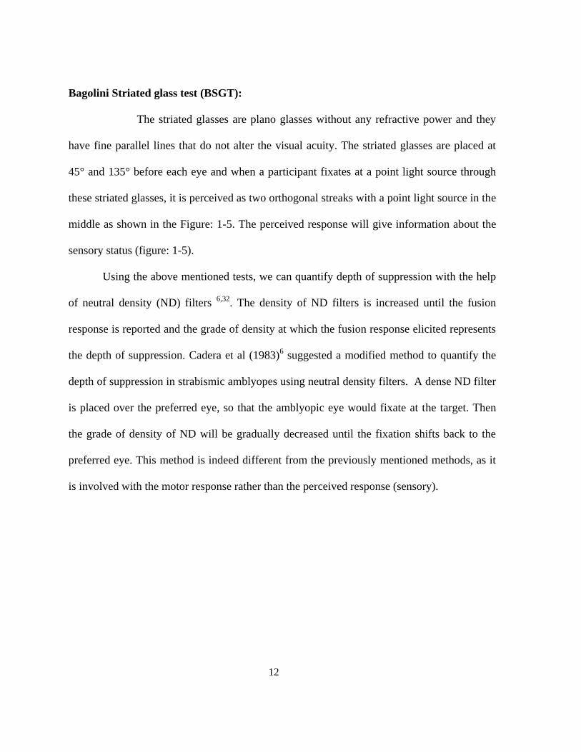
Bagolini Striated glass test (BSGT):

The striated glasses are plano glasses without any refractive power and they

have fine parallel lines that do not alter the visual acuity. The striated glasses are placed at

45° and 135° before each eye and when a participant fixates at a point light source through

these striated glasses, it is perceived as two orthogonal streaks with a point light source in the

middle as shown in the Figure: 1-5. The perceived response will give information about the

sensory status (figure: 1-5).

Using the above mentioned tests, we can quantify depth of suppression with the help

of neutral density (ND) filters 6,32

. The density of ND filters is increased until the fusion

response is reported and the grade of density at which the fusion response elicited represents

the depth of suppression. Cadera et al (1983)6 suggested a modified method to quantify the

depth of suppression in strabismic amblyopes using neutral density filters. A dense ND filter

is placed over the preferred eye, so that the amblyopic eye would fixate at the target. Then

the grade of density of ND will be gradually decreased until the fixation shifts back to the

preferred eye. This method is indeed different from the previously mentioned methods, as it

is involved with the motor response rather than the perceived response (sensory).

13

Figure 1-4 Different precieved response of Worth four dot test

The figure showing the possible perceived response, b) fusion: usually seen in orthophoria or anomalous

retinal correspondence, c) Left eye suppression, d) Right eye suppression and e) uncrossed diplopia seen

in esotropia. (Image adapted from von Noorden, 2002)

Figure 1-5: Perceived responses from BSGT

a) showing fusional response seen in normal retinal correspondence or anomalous retinal response, b)

Right eye suppression, c) central suppression and d) diplopia (Image adapted from von Noorden, 2002).

1.3 Amblyopia

1.3.1 Definition and types

The term amblyopia literally means “dull vision” (ambly – dull). Von Graefe crudely

defined it as “the condition in which the observer sees nothing and the patient very little”56

.

14

However it is scientifically defined as a “decrease in visual acuity in one eye when caused by

abnormal binocular interaction or occurring in one or both eyes as a result of pattern vision

deprivation during immaturity, for which no cause can detected during the physical

examination of the eyes and which in appropriate cases is reversible therapeutic measures 56

.

Amblyopia is classified into three groups based on the etiology; strabismic amblyopia,

anisometropia amblyopia and visual deprivation (amblyopia ex anopsia)11,21,56

.

1.3.2 Amblyopia and Suppression

It should be noted that suppression plays a major role in the amblyopia. In other

words, all amblyopes would have suppression but not vice versa. For example, alternating

strabismics would have suppression to avoid diplopia or confusion. Since they have

alternating fixation, they might not have amblyopia. There are two different schools of

thought on amblyopia and suppression. The first school of thought suggests that suppression

is a consequence of amblyopia. Indeed, Holopigian et al20

showed a negative correlation

between amblyopia and suppression, i.e. greater the amblyopia; the less suppression is

needed to eliminate the binocular summation. The second school of thought suggests that

amblyopia is a consequence of suppression. In this scenario, the suppression develops due to

a disruption in binocular function (either because of strabismus or anisometropia). However,

Li et al, 2011 32

have measured the degree of suppression using global motion technique in

43 amblyopic (strabismic and anisometropic) patients and showed a positive correlation

between amblyopia and suppression. They also have also argued that the results of

Holopigian et al (1987) was because of their 10 participants, only of whom had visual acuity

worse than 20/30 in the amblyopic eye.

15

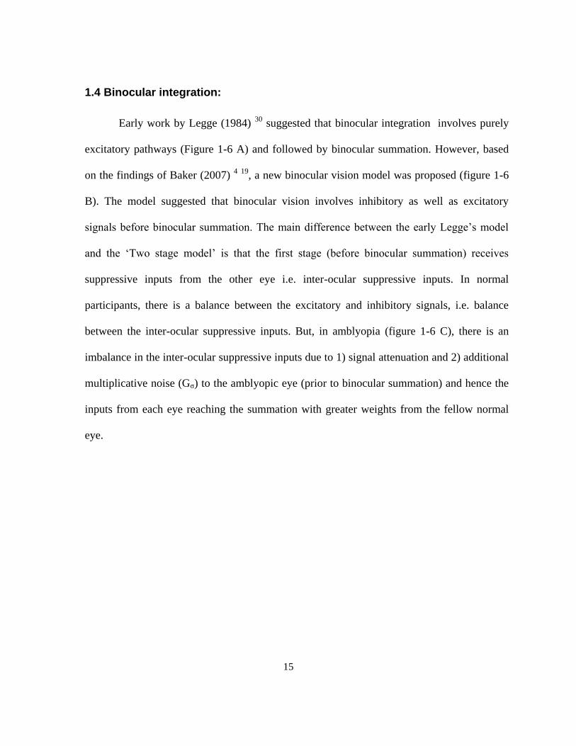
1.4 Binocular integration:

Early work by Legge (1984) 30

suggested that binocular integration involves purely

excitatory pathways (Figure 1-6 A) and followed by binocular summation. However, based

on the findings of Baker (2007) 4 19

, a new binocular vision model was proposed (figure 1-6

B). The model suggested that binocular vision involves inhibitory as well as excitatory

signals before binocular summation. The main difference between the early Legge’s model

and the ‘Two stage model’ is that the first stage (before binocular summation) receives

suppressive inputs from the other eye i.e. inter-ocular suppressive inputs. In normal

participants, there is a balance between the excitatory and inhibitory signals, i.e. balance

between the inter-ocular suppressive inputs. But, in amblyopia (figure 1-6 C), there is an

imbalance in the inter-ocular suppressive inputs due to 1) signal attenuation and 2) additional

multiplicative noise (Gσ) to the amblyopic eye (prior to binocular summation) and hence the

inputs from each eye reaching the summation with greater weights from the fellow normal

eye.

16

Figure 1-6: Models of binocular vision

A) Legge’s model of binocular vision which shows just summation. B) Two stage of normal participants.

C) Two stage model of amblyopes. p,q,m are excitatory components; G – noise generator; L – left eye; R

– Right eye; Green lines represent excitatory signals and red lines represent inhibitory signals (Mansouri

et al, 2008) [Copyright obtained – Appendix C].

Binocular summation:

The binocular summation ratio is the ratio of binocular to monocular sensitivities 4. It

is an indication of binocular advantage and is often measured using sine wave gratings 4,30

.

This ratio for the normal observers will be around √2 (≈1.4), i.e. typically higher than

summation of the two monocular signals 7. If the ratio is unity, then there is no binocular

advantage and this is the scenario in the amblyopic observers. Thus the amblyopic observers

17

have lower binocular summation (near unity) at higher spatial frequencies which led to a

conclusion that binocular summation of contrast is absent 42

. The reason for reduced/absent

of binocular summation might be due to the loss of binocular cortical neurons. But recently a

study done by Baker et al (2007)4 suggested that in human amblyopes, the absence of

binocular summation is due to the substantial difference between the monocular threshold of

dominant and non-dominant eyes. They also added that binocular summation could be

achieved by attenuating the signals to the normal eye, i.e. reducing the contrast of images to

the dominant eye. But the question is how much of the contrast is to be reduced to the

dominant eye in order to achieve binocular summation, i.e. how much of the contrast has to

be reduced to achieve that balance point between two eyes. This balance point can be found

be the technique called ‘Motion Coherence threshold’.

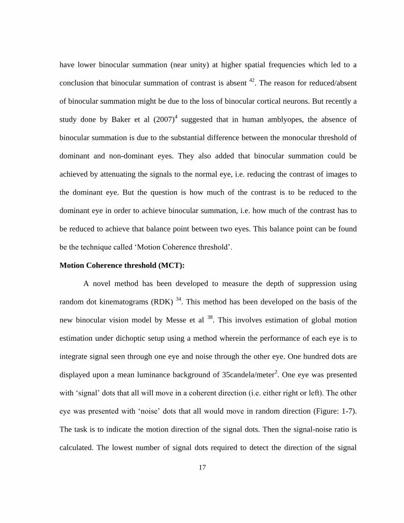
Motion Coherence threshold (MCT):

A novel method has been developed to measure the depth of suppression using

random dot kinematograms (RDK) 34

. This method has been developed on the basis of the

new binocular vision model by Messe et al 38

. This involves estimation of global motion

estimation under dichoptic setup using a method wherein the performance of each eye is to

integrate signal seen through one eye and noise through the other eye. One hundred dots are

displayed upon a mean luminance background of 35candela/meter2. One eye was presented

with ‘signal’ dots that all will move in a coherent direction (i.e. either right or left). The other

eye was presented with ‘noise’ dots that all would move in random direction (Figure: 1-7).

The task is to indicate the motion direction of the signal dots. Then the signal-noise ratio is

calculated. The lowest number of signal dots required to detect the direction of the signal

18

dots represents ‘motion coherence threshold’ (MCT). The threshold would also be measured

at 5 contrast offsets between the two eyes with signal is presented to the dominant eye or the

non-dominant eye. The contrast ratio to the non-dominant eye is always fixed at 80-100%

whereas the contrast ratio to the normal eye varies. Then the MCT of the dominant eye and

the non-dominant eye would be plotted as a function of contrast ratios (figure: 1-8). Then the

plots would be fitted linearly for the dominant eye and the non-dominant eye separately. The

intersection of the two linear fits represents the ‘balance point’34,58

.

Figure 1-7: Random dot kinematograms (RDK).

One eye (Image on the right) seeing the signal dots (moving in a coherent direction) and the other eye

seeing the noise dots (moving in random direction) (Zhang et al, 2011).

Figure 1-8: Balance point calculation.

-5

0

5

10

15

20

25

30

35

0 20 40 60 80 100 120Mo

tio

n c

oh

ere

nce

th

resh

old

Contrast ratio

Balance point in Control participant (Non dominant eye contrast - 60)

AME thres

FFE thres

Linear (AME thres)

Linear (FFE thres)

19

The MCT of the dominant eye and the non-dominant eye was plotted as a function of contrast ratio. The

intersection of the two linear fits represents balance point (Zhang et al 2011).

The balance point has a significant role in this thesis. This research thesis is about the eye

movements in strabismics amblyopes, especially challenging their fixational eye movements

and fusional vergence, once their strabismus is optically aligned and the interocular

suppression is eliminated by attenuating the signal from the dominant eye.

20

Chapter 2: FIXATION EYE MOVEMENTS IN NORMALS AND

AMBLYOPES

2.1 Introduction

Eye movements are of two main types: those that stabilize the image on the fovea

(vestibular, visual fixation, optokinetic and smooth pursuit) and those that bring image on to

the fovea (nystagmus quick phase, saccades and vergence) 31

. There are six types of extra

ocular muscles which facilitate these eye movements: four rectus muscles (superior, inferior,

medial and lateral) and two oblique muscles (superior and inferior) 26,56

.

To see a stationery object best, image should be held on fovea. But it has been known

since the 18th

century that our eyes are never still even during fixation. The main goal of the

oculomotor fixation eye movement is not just retinal image stabilization but also to prevent

image from fading out (Troxler’s effect) by optimal image motion 36

. There are three types of

eye movements that occur during visual fixation: ocular tremors, drifts and microsaccades

9,11,36,37.

2.1.1 Fixation in normals:

Tremors:

Otherwise called as physiological nystagmus and defined as an “aperiodic, wave like

motion of the eyes with a frequency of approximately 90 Hz” 36

. This is the smallest of all eye

movements and is difficult to measure as the amplitude (0.01°) 31

of tremors is usually in the

range of the recording system’s noise 36

. The contribution of tremors in the maintenance of

21

vision is not clear as the frequency of the tremors is much higher than flicker frequency

threshold. Tremors are thought to be independent in the two eyes 36

.

Ocular Drifts:

“Drifts are small and slow movements which occur simultaneously with tremors and

take place between microsaccades” 36

. Drifts are thought to be random eye movements that

are generated by instability of the oculomotor system. It could also be a restoring elastic

force of extra ocular muscles which pulls away the eye from its position 36

.

Microsaccades:

“Microsaccades are involuntary jerk-like fixation eye movements that occur 3-4 times

per second” 36,37

. They are the largest and the fastest among all three fixational eye

movements. They are typically less than a third of a degree and can be suppressed during

visual tasks that demand steady fixation like threading a needle. The amplitude of

microsaccades is not the only criterion to differentiate it from normal voluntary saccades,

because the normal voluntary saccades can also be made to such small degrees 13,31

.

Microsaccades are involuntary and occur only when the person attempts to fixate an object.

Like normal voluntary saccades, the microsaccades do follow ‘main sequence’ 31

. The role of

microsaccades in visual perception is not clear. However, recent studies suggested that the

microsaccades increase the refresh rate to counteract receptor adaptation. On the contrary,

there are studies which consider these fixational eye movements as random eye movements

and not goal-directed29,55

. Based on this, they developed a stochastic model on fixational eye

movements55

.

22

The stability of fixation eye movements was first measured by Krauskopf, Riggs et al

(1959)27

and they showed that under monocular and binocular viewing conditions, these eye

movements are very precise and variations are small, being less than 3’. Steinman et al

(1982) 51

and Ott et al (1992) 41

have also measured the stability of fixational eye

movements. Ott et al (1992)41

have measured mean and standard deviation of binocular

fixation eye movements to quantify the stability of fixation and he found; for horizontal

fixation eye movement: 0.11°±0.05°, for vertical fixation: 0.15°±0.07°. Kruaskopf et al

(1960) 27

have also measured correlation between the horizontal eye positions of two eyes.

They sampled few eye position data without any microsaccades and found poor correlation.

Hence they concluded that ocular drifts are uncorrelated and non-conjugate. Then, they

sampled eye positions including microsaccades and found correlation coefficients to be

around 0.34 to 0.52. Therefore they concluded that the microsaccades are the main source for

correlation between two eyes.

2.1.2 Fixation eye movements in amblyopes:

Ciufredda et al (1979) 10

measured and evaluated fixational eye movements in

strabismic and anisometropic amblyopes and qualitatively noted four abnormal patterns of

eye movements during fixation; increased ocular drifts, saccadic intrusions latent nystagmus

and manifest nystagmus. The average amplitude of the ocular drifts seen in the amblyopic

eyes was 0.7 degrees (peak to peak drift amplitude even as high as 3.5 degrees) which is

higher than the amplitudes of drifts seen in normal eyes. They have also found drifts

accounting for 75% of the total fixation time in amblyopes without strabismus, 50% of the

total fixation time in constant strabismic amblyopia and 20% of the total fixation time in

23

intermittent strabismus. Hence they concluded that amblyopia (rather than strabismus) was

the factor responsible for increased drifts (as drifts seen in the group of amblyopes for 75%

of time). In amblyopes, saccadic intrusions mean amplitude was 0.7 degrees with a range of

0.25 – 5 degrees (saccadic intrusions are horizontal saccades which results in net change of

the eye position). Saccadic overshooting (the primary saccade has larger amplitude than

required) and glissadic undershooting (slow drifting eye movement) were also observed in

amblyopes 10

. Similar to normal eyes, the saccades in the amblyopic eyes could be controlled

during visual attention and fixating small targets. But the information of fixation stability was

missing.

Stability of fixation eye movements in amblyopes:

Recently Gonzalez et al (2012)13

have used the measure called Bivariate Contour

ellipse area (BCEA) to quantify the stability of fixational eye movements. Gonzalez et al

(2012) 13

quantified the stability of fixation in amblyopes and normal binocular vision

participants. They calculated BCEA (bivariate contour ellipse area) to quantify the stability

of fixation. The BCEA value represents region/area of fixation over which the eye positions

are found for a 68.4% of the time and this value has been used to quantify stability of fixation

(further details on calculation of BCEA are in methods section) 13,50,52–54

. The smaller BCEA

value indicates better fixation stability. In normal participants, Gonzalez et al (2012)13

found

that fixation stability was better with binocular viewing compared with monocular viewing.

In amblyopes, they found poor fixation stability with amblyopic eye viewing and also

relatively poorer fixation stability with binocular viewing than found in normal participants.

Hence, concluded that binocular summation has bigger role in fixation stability.

24

Interestingly, it has been established that oculomotor aspects get normalized after

successful amblyopia therapy. Ciufredda et al (1979) showed that eye movement aspects like

ocular drifts amplitude, glissadic undershoots, steady fixation and pursuit gain get

normalized after successful amblyopia treatment10

. However, some oculomotor aspects do

not become normalized; these functions include saccadic latency and saccadic overshooting.

But all of his findings were on only one subject who showed stereopsis improved from 800

arc seconds to 60 arc seconds and visual acuity to 6/6. It is important to distinguish a

monocular improvement in visual acuity from binocular integration. In the case of strabismus

the latter may never be achieved in all cases. While in the case of anisometropic amblyopia

binocular vision can be restored but typically well after the amelioration of amblyopia.

25

Chapter 3: OBJECTIVE OF THE STUDY

Many novel anti-suppression therapies like balanced contrast techniques 18

have

evolved which attempt to improve binocular functions like stereopsis. This is unlike

traditional patching therapy where monocular function like visual acuity is targeted. They

have also noted significant improvement in visual acuity of the amblyopic eye and also

notable improvement in stereopsis when the suppression is reduced with balanced contrast

between the normal eye and the amblyopic eye (i.e. with binocular summation). But little is

known about the effect of the aforementioned ‘balance point’ on oculomotor aspects.

It has been well established that oculomotor functions like visual fixation and

disparity vergence in the amblyopes are poor 5,9,13,25

. They have all listed that lack of

binocular summation or loss of binocularity due to foveal suppression as the reasons for poor

oculomotor control. But it is unclear what underlying mechanism (sensory or motor aspects)

is responsible for producing such abnormal movements. It is also unclear whether the lack of

foveal stimulation or lack of binocular summation is causing this poor fixation stability and

this study will try to address all of these research questions. Hence we hypothesize that the

stability of fixation should improve if we align the strabismus (i.e. bi foveal stimulation) and

eliminate the inter-ocular suppression (reducing the contrast to the fellow fixing eye, thereby

facilitating balanced monocular inputs).

26

Chapter 4: INSTRUMENTATION AND METHOD

To test our hypothesis, we had to consider three things: 1) optical alignment of the

angle of strabismus, 2) elimination of inter-ocular suppression in the strabismic patient and 3)

measurement of resulting eye movements.

4.1 Ocular Alignment

A haploscope was designed to optically align the eyes while strabismic subjects

dichoptically viewed two similar targets imaged onto two LCD monitors (9”Lilliput®) which

were placed at the distal end of each haploscope arm. The participants viewed the monitors

through two front-surface mirrors (2” x 3”) placed orthogonally at 10cm from the lateral

canthus and 30 cm from the monitors. Thus, the total optical length was 40 cm for each arm.

(Figure: 4-1a and 4-1b). Chin and forehead rests was clamped at 10 cm from the mirrors. To

stabilize head movement, the participant’s head was strapped along with forehead rest using

Velcro strap. Two monitors on the haploscope were controlled by a MacIntosh laptop and

resolution of the secondary monitors (haploscope monitors) was set to 1600x600 pixels.

Using an external multi-display adapter (DualHead2Go, Matrox®), the resolution of the

secondary monitors was split into two such that each monitor shared 800x600 pixels

resolution. The gamma correction for our haploscope monitors was found to be 2.2. See the

Appendix-I for more details.

27

Figure 4-1: Schematic and actual picture of the haploscopic setup

28

As mentioned before, the main purpose of the haploscope is to optically align the

strabismic patients. The reason for using haploscope over a prismatic correction is that 1)

dichoptic setup (information from each eye can be evaluated better) and 2) attenuation of the

signal to the normal eye can be done efficiently (i.e. contrast to the fellow fixing eye can be

reduced easily).

4.1.1 Calibration of the haploscope

The angular scale of the haploscope needed to be calibrated for actual eye movements

as the centers of rotation of the haploscope arms do not coincide with the center of rotation of

the eyes. Dissimilar targets, a big white circle on a black background in one screen and a

small black circle on a white background, were used in order to avoid the influence of

fusional vergence (Figure: 4-2). A known amount of ophthalmic prism (15∆ - 45∆ base out)

was placed in front of one of the eyes so that it would induce saccadic eye movement (since

it is a dissimilar object, fusional vergence would not be induced) by displacing one of the

images. Then the arm of the haploscope was rotated until the participant reported that the

images overlapped. The degree of rotation was noted and then the same procedure was

repeated for other prisms. Six normal participants volunteered for this calibration process.

The results showed that the empirical values (haploscope rotation) are always higher

than the calculated values (actual eye rotation). The variation in the results could be due to

the inter-participant difference in the mirror-to-eye distance. The results were shown in the

Table 4-1 and in the figure: 4-3.

29

Prism

given

Correspondin

g

Degrees

(Calculated)

Degree of

rotation in

the haploscope (Empirical)

Participant

1

Participant

2

Participant

3

Participant

4

Participant

5

Participant

6

25 14.0 15.00 14.33 11.33 19.33 16 15

30 16.7 18.33 16.83 14.50 24.17 18 18

35 19.3 19.83 19.17 19.17 28.33 21.5 21.5

40 21.8 23.67 22.33 22.17 29.67 24 24

45 24.2 25.50 25.33 29.67 31.33 29 26

Table 4-1: Values of the calculated and the empirical values of eye rotation.

The values clearly show us that the empirical values (haploscope rotation) are always higher than the calculated

values (actual eye rotation). The calculated values were determined according to the power of the ophthalmic

prisms, e.g. 25∆ would shift the image such that the eye would rotate ~14°.

Figure 4-2: Empirical (measured eye rotation) values as a function of calculated values (actual eye rotation) Error

bars represent 1 SD.

Figure 4-3: Dissimilar target used for the calibration of haploscope.

y = 1.2328x - 2.2213

10

15

20

25

30

35

10 15 20 25

Me

asu

red

de

gre

e

(Hap

losc

op

e r

ota

tio

n)

de

gre

es

Actual degree (Eye rotation) degrees

Calculated vs. empirical values

Linear (Calculated)

Linear (Empirical)

30

A big white circle on black background (right eye) and a small black circle on a white background (left eye).

Conclusion:

The results of this calibration have suggested that the arms of the haploscope should be

rotated 1.2x times the degree to induce the required degree of eye movement. In other words,

if we rotate the arm of the haploscope 5 degrees (according to the haploscope’s scale) then it

would induce approximately 3.5° ocular rotation only. However, the ocular alignment could

be done efficiently using this haploscope. By doing alternating cover test while aligning the

objective angle of the strabismus, we could make sure that the targets were bi-foveally

fixated.

4.2 Attenuating inter-ocular suppression:

As explained in the previous chapter, binocular summation could be achieved in

amblyopes if the contrast of the image to the fellow fixing (normal) eye was attenuated. A

stimulus was designed (figure: 4-4).

Figure 4-4: Stimulus for fixational and vergence eye movments.

31

Each target (box) shown to the each eye and when a participant fuses the images, it will appear as a single

outer box with a single cross in the middle with four dots. The dots were to check suppression during the

trial.

4.2.1 Description of the stimuli:

The stimulus was created using the software, Psychtoolbox, MATLAB (Mathworks,

Inc. ®)44

[Dr. Jiawei Zhou, McGill University, QU, Canada, Personal communication, 29th

Mar, 2012]. The stimulus had outer box which subtended 11.3° visual angle at 40 cm

whereas the middle cross subtended 2.3° visual angle at 40 cm. Under dichoptic setup, each

eye would see only two dots and these dots were used as suppression checks. So if a

participant fused the stimulus (under dichoptic setup); he/she should see a single outer box

with a single cross in the middle with four dots. The stimulus was shown on a gray

background so that the contrast of the outer box, the cross and the dots could be varied on

either side, i.e. increase/decrease the contrast easily using Weber’s contrast43

.

4.2.2 Reducing contrast of the stimulus to the fellow fixing (normal) eye:

Contrast was defined as the Weber ratio of the difference between luminance of the

feature and background to the luminance of the background (Equation-1) 43

.

I – luminance of the feature and Ib – luminance of the features (here, the outer box, the cross

and the dots). Weber’s contrast is usually preferred over Michelson contrast in the cases

where the small features are presented over the uniform background. In the code (Matlab)

(Appendix-C), the luminance was defined as the scale of 0 to 1, where 0 is black and 1 is

32

white. The background was set gray i.e. 0.5 in the luminance scale. For example, in order to

set the contrast of the image to 20% (i.e. reducing 90%), the value of ‘I’ should be 0.1 and

‘Ib’ should be as always 0.5. Substituting these values in the above equation would set the

contrast of the image at 20% (For detailed description of Weber’s contrast and calculation,

please refer Appendix-B).

4.3 Measuring eye movements:

A binocular infra-red eyetracker (ViewPoint EyeTracker® PC-60, Arrington

Research Scottsdale, USA) was used to track the eye movements. Eye movements were

sampled at the rate of 60Hz (High Speed Wide mode) which has been shown to be

sufficient for measuring vergence eye movements 45

. The specifications of the eyetracker are

summarized in the table 4-2. The eyetracker was mounted on a spectacle frame as shown in

the figure: 4-5. The spectacle frame was big enough to fit over participant’s own prescription

glasses.

Parameters Specification

Eye tracker type Video based infrared eye tracker

Tracking method Dark pupil method

Sampling frequency 60Hz (High Speed Wide mode)

Range of measurement Horizontal: ±44°

Vertical: ±20°

Spatial resolution 0.15°

Accuracy (as noted in the user manual) 0.25° - 1°

Table 4-2: Specification of the eyetracker

33

Figure 4-5: Eyetracker mounted on a spectacle frame.

Eye movements data were collected using software Viewpoint®, Arrington Research

and analyzed using software called ‘ILab’ 12

. This is free software and available online

(http://www.brain.northwestern.edu/ilab) which was created by Dr. Darren Gitelman,

Northwestern University Medical School, Chicago, Illinois.

4.3.1 Setting up Eyetracker to measure eye movements:

To measure eye movements, the eye tracker parameters were adjusted according to

our instrumental setup. The information like total viewing distance (here, 40cm) and

resolution of the stimulus window (Haploscope monitor resolution, 1600x600) were entered

in the software. After entering this required information, the participant was asked to wear

the eyetracker and the care was taken to make sure that the eye tracker was positioned firmly

without sliding down. If required, a sponge was used to provide extra support to hold the

34

eyetracker firmly. Then the camera and the IR LED of each eye were adjusted such that pupil

of the eye was tracked properly as shown in the figure: 4-6. Then the participant was asked to

place his/her chin on the chin rest and asked to keep the forehead firm against the forehead

head rest. At this position, the participant head was strapped along with the chinrest to

minimize the head movement during the experiment.

4.3.2 Calibration of the eye tracker:

Calibration of the eyetracker was done by measuring the eye position at the

predetermined 16 points in the stimulus window (i.e. Haploscope monitor screen). The

calibration stimulus is shrinking motion of green rectangular frames (figure: 4-7) which

appear randomly in the sixteen predetermined points. A good calibration is checked by

looking at the arrangement of calibration point and is indicated by a relatively rectilinear and

well separated configuration dots as shown in the figure: 4-7.

35

Figure 4-6: interface of software Viewpoint®.

The top left (Eye camera window) is the picture of eyes getting illuminated by IR LED (dark pupil method). Eye A

represents right eye and Eye B represents left eye. The top right is the stimulus window for user reference. The

bottom right is the pen plot window where real-time vergence, x and y gaze points, velocity are seen. The left bottom

is the calibration window where the settings of the calibration and calibration check can be seen.

Figure 4-7: Stimulus for calibration of eye tracker.

a) (Left image) shows the calibration stimulus shrinking green square frames and b) shows a calibration

points which are well spaced and relatively rectilinear indicating good calibration.

36

4.4 Participant selection:

Seven strabismic participants [5 esotropes and 2 exotropes] [Mean age: 29.17±9.47

years] [Mean visual acuity: AME = 0.39±0.13; FFE = -0.13±0.04] were recruited from the

School of Optometry Clinic, University of Waterloo and informed consent was obtained

from each participant. Relevant clinical details like visual acuity, sensory status (Worth’s

four dot test, Bagolini striated glass test and Random dot stereogram) and motor status (cover

test and prism bar cover test) were collected. The details are tabulated in the table-1. Then the

motion coherence test (Zhang, 2011)58

was performed to measure balance point contrast

ratio. However the contrast was fixed finally at the level where the participant had subjective

response of constant fusion. It should be noted that all of our strabismic participants had

central suppression with the Bagolini striated glass test (BSGT). In the case, if they had any

form of ARC, then they would have experienced diplopia when they were aligned to their

objective angle. Hence, the main inclusion criterion was that the strabismics should have at

least central suppression with BSGT such that they would not experience any diplopia when

their objective angle of strabismus was corrected and a balance point could be empirically

measured. One participant (ON) was then excluded from the study, as a balance point could

not be established since the participant could not perform motion coherence test nor

subjectively respond well for contrast changes between FFE and AME. The remaining six

subjects were included in the study.

Fixational eye movements were then measured in four different conditions; 1)

Unaligned/high contrast [ strabismus unaligned and at 100% contrast target to both eyes

(i.e. no bi-foveal stimulation and no binocular summation)], 2) Unaligned/balance point

37

[strabismus unaligned but with balance point contrast (i.e. no bi-foveal stimulation but

binocular summation)], 3) Aligned/high contrast [objective angle of strabismus aligned but

at 100% contrast target to both eyes (i.e. bi-foveal stimulation but no binocular summation)]

and 4) Aligned/balance point [objective angle of strabismus aligned and balance point

contrast target (i.e. bi-foveal stimulation and binocular summation)].

Figure 4-8: Four different viewing conditions used to measure fixational stability.

Ocular alignment for subject angles was achieved by applying the principles of the

Douse Target Test used in synoptophore testing of strabismics. The subject’s head was

placed in the synoptophore. Each eye dichoptically viewed a cross which was displayed on

both screens. An alternate cover test was performed in order to assess the direction of the

strabismic angle. One arm of the haploscope was adjusted in order to reduce the deviation.

Strabismus – unaligned

Contrast – 100% target contrast to both eyes

Strabismus – unaligned

Contrast – 100% target contrast to the amblyopic eye and reduced contrast to the normal eye

Strabismus –aligned to objective angle

Contrast – 100% target contrast to both eyes

Strabismus –aligned to objective angle

Contrast – 100% target contrast to the amblyopic eye and reduced contrast to the normal eye

Balanced Input

No Yes

No

Yes

Bi-Foveal

stimulation

38

Using a method of limits a point was reached when there was no movement seen in the cover

test. The subject then identified if the crosses where superimposed. If not, ARC was

suspected and the subject reset the arms in order to note the angle of ARC. In cases however,

testing commenced from the objective angle of the strabismus i.e. that determined by

neutralization of the cover test. Then, the eye tracker was calibrated as described above and

the eye movements were measured while the participants fixated each dichoptic targets for

continuous 5 minutes. The target was as shown in the Figure: 4-2. The subjective response of

each participant was noted in every condition to know the sensory status with particular

condition (by asking ‘how many dots and crosses are visible’) so that we would know

whether they had either suppression or fusion. These procedures were repeated for every

strabismic participant but the orders of the above mentioned conditions (Figure: 4-1) were

randomized for each participant.

For normal participants [Mean age: 25.3±4 years] [Mean Visual acuity: -0.1±0.08],

the haploscope arm was rotated to certain degree where accommodation and vergence lie in

the same plane, i.e. vergence demand for 40 cm according to their inter-pupillary distance.

Once calibration of the eye tracker is done, the fixation eye movements were measured for 30

seconds in three conditions which was more likely representing strabismus participants; 1)

right eye viewing the target and the left eye viewing no target, 2) left eye viewing the target

and the right eye viewing no target and 3) binocular viewing. Then the results of both groups

were compared.

39

Figure 4-9: Target for the participants (normals and strabismics) to fixate with equal contrast to both

eyes.

Figure 4-10: Target for the strabismic participants to fixate with balanced (reduced) contrast to the

fellow eye

Analysis of data:

The collected data were analyzed using the software called ‘Ilab’. It was used to

convert eye positions from screen coordinates (from Viewpoint) to degrees and also to

remove blinks. The blinks were removed based on the criterion of axis limits, i.e. the

coordinates were already set according to the resolution of the haploscope monitors

40

(1600x600); if the eye position exceeds these axis limits, then it was considered as a blink

and removed from the data. Five data points were also deleted pre and post blink. Once the

blinks were deleted, the horizontal and vertical eye positions were converted from screen

coordinates to degrees and exported to MS Excel. Then the eye positions of each eye were

plotted as a function of time. Stability of fixation eye movement was then measured for each

eye by calculating global BCEA.

Fixational stability:

The measure of global BCEA (bivariate contour ellipse area) was used to measure the

stability of fixation in normal and strabismus participants. The BCEA value represents the

region/area of fixation over which the eye positions are found for a 68.2% of the time and it

is calculated using the following equation,

where σx and σy are standard deviation of the horizontal and vertical eye position, ρ is the

Pearson’s correlation between the horizontal and the vertical eye positions during the trial

and χ2 = 2.291 is the chi-square value (2 degree of freedom) corresponding to a probability

value of 0.682(i.e.±1SD). The smaller BCEA value indicates better fixation stability. The

BCEA values were transformed into log values to get normality.

41

Participant Refraction Visual acuity Sensory status Strabismus Amblyopic

eye OD OS WFDT BSGT Stereopsis D N

XU

41/M

OD:+6.75/-2.50x30

OS:+5.00/-1.75x162

0.42 -0.08 D: Intermittent suppression

N: Fusion

Central

Suppression

(OD)

No gross

stereopsis

10 PD RET 12 PD RET OD

MA

27/M

OD:+2.50/-1.25x20

OS: plano

0.54 -0.14 D: Uncrossed

Diplopia

N: Fusion

Central

Suppression

(OD)

No gross

stereopsis

8 PD RET 14 PD RET OD

ON

20/F

OD:+0.50

OS:+4.50/-1.00x35

-0.12 0.2 D & N: Fusion Central

Suppression

(OS)

No gross

stereopsis

8 PD LET 12 PD LET OS

OT

22/M

OD:-1.00

OS:-1.00/-0.25x160

-0.1 0.34 D & N: Fusion Central

Suppression

(OS)

200 arc sec 4 PD LET 4 PD LET OS

ST

24/F

OD:-2.75/-0.75x25

OS:-3.25/-1.25x10

0.52 -0.12 D & N: Fusion Central

suppression

(OD)

200 arc sec 6 PD RXT 6 PD RXT OD

MT

42/M

OD:-2.75/-1.00x105

OS: -2.75/-1.00x80

0.34 -0.2 D: Intermittent suppression

N: Fusion

Central

suppression

(OD)

No gross

stereopsis

6 PD RET 8 PD RET OD

AD

40/M

OD:-1.00

OS: plano

1.12 -0.1 OD: Suppression OD:

Suppression

No gross

stereopsis

6 PD RXT 6 PD RXT OD

Table 4-3: Details of sensory and motor status of the participants

Abbreviations used: WFDT – Worth four dot test, BGST – Bagolini striated glass test, D – Distance, N – Near, PD – prism dioptres, RET – Esotropia, LET – Left esotropia, RXT

– Right exotropia

42

Chapter 5: RESULTS

5.1 Qualitative analysis of fixation pattern:

5.1.1 Fixation pattern in normals:

As noted earlier, the stability of fixation was measured under three different

conditions. In the monocular condition, fixation was more stable in the eye which was

viewing the target than the covered eye (Fig: 5-1). Under binocular conditions, both eyes had

same pattern of visual fixation (Fig: 5-2).

Figure 5-1: Monocular viewing eye trace of normal participant

Blue line and red line represents right eye and left eye respectively. OD was viewing the monitor covered

with black sheet of paper whereas the OS was viewing the target. These eye traces show the non-viewing

eye (here OD) with poor fixation.

Figure 5-2: Binocular viewing eye trace of normal participant

-15

-10

-5

0

0 500 1000 1500 2000 2500

Eye

po

siti

on

(d

egr

ee

s)

Time (ms)

Monocular Viewing

OD

OSviewing

-15

-10

-5

0

0 500 1000 1500 2000 2500

Eye

po

siti

on

(d

egr

ee

s)

Time (ms)

Binocular viewing

OD

OS

43

Traces of horizontal eye position of a normal participant while both eyes viewed the target. Blue line and

red line represents right eye and left eye respectively. Fixation of both eyes appeared to be as stable as

that of the viewing eye in monocular condition (p=0.99)

5.1.2 Fixation patterns in strabismic amblyopes:

The eye movement traces of two (XU and ON) of the six strabismic participants under four

different conditions are shown in the Fig: 5-3 and Fig: 5-4. The traces have suggested that in

an unaligned position, the fellow fixing eye (FFE) was holding fixation whereas the

amblyopic eye (AME) showed poor fixation with higher amplitude of drifts. But the fixation

was improved when the objective angle of strabismus was aligned i.e. bifoveal fixation. The

fixation was even better when the strabismus was aligned and also when the contrast was

balanced between FFE and AME.

-20

-10

0

10

20

0 50 100 150 200 250 300 350

Eye

po

siti

on

(d

egr

ee

)

Time ( sec)

a) Unaligned/High contrast

AME Hori

FFE Hori

-15

-5

5

15

0 50 100 150 200 250 300 350

Eye

po

siti

on

(d

egr

ee

s)

Time (sec)

b) Unaligned/Balance point

AME Hori

FFE Hori

44

Figure 5-3: Fixation eye trace of the participant XU.

The traces show the horizontal eye position of the amblyopic eye (AME) and the fellow fixing eye (FFE)

over the first 5 minutes of viewing. The conditions are listed as follows (from top to bottom):

Unaligned/high contrast, Unaligned/balance point contrast, Aligned/high contrast and Aligned/balance

point. Blue lines represent eye traces of the amblyopic eye (AME) and brown lines represent eye traces of

the fellow normal eye (FFE). The eye traces show that the quality of fixation was poorer at the unaligned

position with greater amplitude of drifts. However, these drifts were reduced and the quality of fixation

improved with the alignment of the eyes and balance point. In the condition of aligned/balance point,

however, the achieved optimal fixation was very transient. After initial period of optimal fixation, higher

amplitudes of drifts were seen.

-15

-5

5

15

0 50 100 150 200 250 300 350

Eye

po

siti

on

(d

egr

ee

s)

Time (sec)

c) Aligned/High contrast

AME Hori

FFE Hori

-15

-5

5

15

0 50 100 150 200 250 300 350

Eye

po

siti

on

(d

egr

ee

s)

Time (sec)

d) Aligned/balance point

AME Hori

FFE Hori

-20

-10

0

10

20

0 100 200 300 400

Eye

po

siti

on

(d

egr

ee

s)

Time (sec)

a) Unaligned/High contrast

FFE Hori

AME Hori

45

Figure 5-4: Fixation eye trace of the participant (OT)

The conditions are listed as follows (from top to bottom): Unaligned/high contrast, Unaligned/balance

point contrast, Aligned/high contrast and Aligned/balance point. Blue lines represent eye traces of the

amblyopic eye (AME) and brown lines represent eye traces of the fellow normal eye (FFE). The eye

traces have shown that the quality of fixation was poorer at the unaligned position with greater

amplitude of drifts. However, these drifts were reduced and the quality of fixation improved with the

alignment of the eyes and balance point. In the condition of aligned/balance point, however, the achieved

optimal fixation was very transient. After initial period of optimal fixation, higher amplitudes of drifts

were seen.

-40

-30

-20

-10

0

0 50 100 150 200 250 300 350

Eye

po

siti

on

(d

egr

ee

s)

Time (sec)

b) Unaligned/Balance point

FFE Hori

AME Hori

-20

-10

0

10

20

0 50 100 150 200 250 300 350

Eye

po

siti

on

(d

egr

ee

s)

Time (sec)

c) Aligned/High contrast

FFE Hori

AME Hori

-20

-10

0

10

20

0 50 100 150 200 250 300 350

Eye

po

siti

on

(d

egr

ee

s)

Time (sec)

d) Aligned/balance point

FFE Hori

AME Hori

46

Under aligned/balance point condition, all strabismic amblyopes could hold optimal

fixation for transient period. This initial period of optimal fixation varied ranging from 30

seconds to 80 seconds (Table: 5-1). Hence initial 30 seconds (where there were no such high

amplitude drifts for every strabismics) was compared with last 3 minutes (where higher

amplitudes of drifts were always seen). The fixation of the AME was better for initial 30

second (Fig: 5-5) (p=0.008).

Subject Period of initial optimal

fixation (sec)

XU 60

MA 38.4

OT 68.3

ST 80

MT 30

AD 42.2

Table 5-1: Period of initial optimal fixation

Initial 30 vs Last 3 min_AME

Initial 30 sec Last 3 min

0.0

0.2

0.4

0.6

0.8

1.0

p=0.008

Log

BC

EA (l

og u

nits

)

Figure 5-5: Initial 30 seconds vs. last 3 minutes

47

The fixation of AME was better for initial 30 seconds where the binocular summation was intact. After

that initial period, higher amplitudes of drifts were seen.

5.2 Quantitative analysis of fixation stability:

The stability of fixation was quantified using two methods; 1) standard deviation of

horizontal eye positions and 2) BCEA.

5.2.1 Standard deviation of Horizontal eye positions (fixation error):

5.2.1.1 Normal observers:

Fixation error in the covered eye (0.6±0.43) was higher than viewing eye in monocular

viewing condition (0.33±0.12) and binocular viewing (0.36±0.1). However, no statistical

significance was found across the conditions [p=0.129].

Figure 5-6: Fixation error in the horizontal eye position of Normal observers.

0

0.2

0.4

0.6

0.8

1

1.2

SD (

de

gre

es)

Viewing eye Covered eye Binocular

Fixation error in the Horizontal eye position

Monocular

48

5.2.1.2 Strabismic amblyopes:

In strabismic amblyopes, on comparing FFE and AME using repeated measures

ANOVA revealed a significant main effect between AME and FFE [F (1, 5) = 17.297;

p=0.009]. Tukey HSD was performed and it showed that the fixational error of AME

significantly reduced when the strabismus was aligned and the contrast was reduced to FFE

(p=0.033). Moreover, under unaligned condition, the fixation error in the AME was

significantly higher than that of FFE (p=0.018). However, the difference between FFE and

AME was reduced when the strabismus was aligned (0.99) (aligned/high contrast) and the

contrast was reduced to FFE (0.987) (aligned/balance point) [Fig: 5-7].

Figure 5-7: Fixational error in the horizontal eye positions of strabismic amblyopes

0.00

0.20

0.40

0.60

0.80

1.00

1.20

1.40

Stan

dar

d d

evi

atio

n in

eye

po

siti

on

(d

egr

ee

)

Unaligned/High contrast Unaligned/balance point Aligned/High contrast Aligned/Balance point

Fixation error in the Horizontal eye positions

AME

FFE

*p=0.018

p=0.99

p=0.987

49

5.2.2 Bivariate Contour Ellipse Area (BCEA):

The values of BCEA were transformed into log values to perform parametrical analysis.

5.2.2.1 Normal observers:

The fixation eye movements were measured for both eyes while one eye fixated the

target and the other eye viewed a uniform black sheet of paper. The results have suggested

that the BCEA of the viewing eye (-0.26±0.25) was statistically significant than the BCEA of

non-viewing eye (0.07±0.33) [p=0.0149]. It implies that viewing eye had better fixational

stability than the non-viewing eye. However, when both eyes were looking at the target, the

fixation stability of both eyes was calculated by averaging the values of right eye and left

eye. The stability of fixation under binocular viewing (-0.24±0.16) was as same as the

viewing eye under monocular condition. The results are shown in the Fig: 5-8.

BCEA_Normals

Monocular Viewing Monocular Covered Binocular [(LE+RE)/2]

-0.6

-0.4

-0.2

-0.0

0.2

0.4

BC

EA

(lo

g u

nit

s)

Figure 5-8: BCEA of normal observers

50

5.2.2.2 Strabismic amblyopes:

In strabismic amblyopes, the results were analyzed in two different ways, 1)

separately for AME and FFE and 2) Binocular BCEA (by averaging the values of FFE and

AME). In strabismic amblyopes, on comparing FFE and AME using repeated measures

ANOVA revealed a significant main effect between AME and FFE [F (1, 5) = 18.697;

p=0.008]. Tukey HSD was performed and it revealed the following results.

AME of strabismic amblyopes:

Fixation stability of AME significantly improved when the strabismus was aligned

(aligned/high contrast = 0.19±0.28) [p=0.015] and it improved further when the contrast was

reduced to FFE (aligned/balance point = 0.018±0.15) [p=0.0009] than unaligned position

(unaligned/high contrast = 0.62±0.3). Though the fixation stability was better after reducing

the contrast to the FFE (aligned/balance point) comparing to aligned/high contrast, there was

no statistical significance (p=0.738) between the two conditions. The results are shown in the

Fig: 5-9. Fixation stability of FFE was always the same under different conditions (Fig: 5-

10).

51

AME_30sec

AME_UA_HC AME_UA_BP AME_obj_HC AME_obj_BP

-0.4

-0.2

-0.0

0.2

0.4

0.6

0.8

1.0

p=0.015

p=0.0009

Log

BC

EA (l

og u

nits

)

Figure 5-9: BCEA of AME

Log BCEA of AME plotted as a function of conditions. The above figure is showing that the BCEA of

AME was better when the objective angle of strabismus was aligned (foveal fixation) than in unaligned

position (p=0.015). The BCEA of AME was even better when strabismus aligned (foveal fixation) and

when the contrast was reduced to FFE (p=0.0009) compared to unaligned position. Abbreviations used:

AME – Amblyopic eye; HC – High contrast; BP – Balance point; Obj – Objective angle aligned; UA –

Unaligned.

FFE_30sec

FFE_UA_HC FFE_UA_BP FFE_Obj_HC FFE_Obj_BP

-1.0

-0.5

0.0

0.5

Log

BC

EA

(lo

g un

its)

Figure 5-10: BCEA of FFE

The quality of fixation of FFE (BCEA) was the same across the conditions. Abbreviations used: FFE –

Fellow fixing eye; HC – High contrast; BP – Balance point; Obj – Objective angle aligned; UA –

Unaligned.

52

Binocular BCEA:

These measures were all under binocular viewing condition and therefore Binocular

BCEA was calculated by averaging the BCEAFFE and BCEAAME. Binocular BCEA values

have also suggested that binocular fixation was more stable when the strabismus was aligned

and the contrast was reduced to FFE (-0.1±0.19) [p=0.0275] than unaligned position

(0.42±0.27).

Bin_BCEA_Initial 30 sec

UA_HC UA_BP Obj_HC Obj_BP-0.2

0.0

0.2

0.4

0.6

p=0.0275

Lo

g B

CE

A (

log

un

its)

Figure 5-11: Binocular BCEA of strabismic amblyopes

Binocular BCEA was calculated by averaging the BCEA of FFE and AME. The same pattern was noted

in Binocular BCEA as well. The binocular fixation was better when the objective angle was corrected.

The binocular fixation was even better when the strabismus was aligned and also when the contrast was

balanced between FFE and AME. Fixation stability was significantly better when the strabismus was

aligned and the contrast was balanced between FFE and AME (Obj_BP).

53

5.2.2.3 Strabismic amblyopes vs. Normal observers:

All conditions for the binocular BCEA of aligned/high contrast and aligned/balance

point were compared with binocular BCEA of normal participants. Statistical significance

was found between aligned/high contrast and normal binocular BCEA (p=0.0205). But no

statistical significance was found between aligned/balance point and normal binocular BCEA

(p=0.1232).

Normals vs Strabs

Strab_HC Strab_BP Normals-0.4

-0.2

0.0

0.2

0.4

p=0.0205

p=0.1232

Bin

_B

CE

A (

log

un

its)

Figure 5-12: Strabismic amblyopes vs. Normal observers

The above results have suggested that the fixation was better and closer to normals only when the

contrast was reduced to FFE (aligned/balance point.

54

5.3 Direction of drifts:

The drifts seen in the strabismic amblyope after aligning the objective angle of

strabismus have the same direction as the direction of strabismus, i.e. strabismics revert back

in the direction of original deviation (Figures 5-11 and 5-12).

Figure 5-13: Direction of drifts in the strabismic participant (XU), an esotrope

Figure 5-14: Direction of drifts in the strabismic participant (AD), an exotrope

The eye traces (figures-5-11 and 5-12) were plotted by difference of the horizontal eye positions of AME and FFE as a

function of time (under the condition of aligned/balanced point); a) XU is an esotrope and showing increase in eso

deviation after initial optimal bi-foveal fixation, b) AD is an exotrope and showing increase in exo deviation after

initial optimal bi-foveal fixation.

0

5

10

15

0 50 100 150 200 250 300 350

Dif

fere

nce

of

Eye

po

siti

on

(d

egr

ee

s)

Time (sec)

a) Drift in stabismic amblyope (XU - esotrope)

-12

-10

-8

-6

-4

-2

0

0 50 100 150 200 250 300 350

Dif

fere

nce

in e

ye p

osi

tio

n

(de

gre

es)

Time (sec)

b) Drift in strabismic amblyope (AD - exotrope)

55

5.4 Correlation of horizontal eye position:

The value of correlation coefficient gives the information of nature of eye movements

and its conjugacy. In other words, high positive correlation suggests that the eye movement is

conjugative [saccadic eye movement] whereas the high negative correlation suggests that the

eye movement is disjunctive. Hence, Pearson’s correlation coefficient between horizontal eye

positions was calculated for every fixational eye movements. The results are tabulated in the

tables: 4-6 (strabismics) and 4-7 (normals).

Participant

STRABISMIC AMBLYOPES

Whole 5 minutes

Initial 30 sec

UA_HC Obj_HC Obj_BP UA_HC Obj_HC Obj_BP

MA -0.28 0.17 0

0.22 0.22 0.4

XU -0.05 -0.87 -0.64

-0.71 -0.8 0.27

OT -0.51 -0.45 -0.4

0.25 -0.6 0.08

ST 0.09 0.37 -0.05

0.26 0.2 0.12

MT -0.14 -0.33 0

0.63 0.65 0.62

AD -0.1 -0.09 0.24

0.32 0.05 0.55

Table 5-2: Correlation coefficients of horizontal eye positions in strabismic amblyopes during fixation

Participants

NORMALS

RE viewing

LE viewing

Binocular viewing

ARH -0.02 0.04 0.2

VJ -0.38 0.06 -0.57

YHH -0.22 0.19 -0.18

SM 0.16 0.57 0.56

RJ -0.52 -0.26 -0.49

CH 0.43 0.54 0.27

Table 5-3: Correlation coefficients of horizontal eye positions in normals during fixation

56

Chapter 6: DISCUSSION

This is the first study to look at the effect of ocular alignment and inter-ocular

suppression attenuation on binocular fixation patterns. As discussed above, Gonzalez et al

(2012)13

used the BCEA analysis to confirm fixation instability under both monocular and

binocular viewing in normal and amblyopic eyes. Control subjects showed significantly

better fixation viewing binocularly compared with monocular viewing. This suggested that

binocular input improved fixation. Fixation of the amblyopic eyes confirmed its high

variability compared to the fellow eye and controls. Unlike the controls, fixation variance

was not significantly improved with binocular fixation. Since the binocular improvement of

fixation was improved only in controls and not the amblyopes, they concluded that the lack

of binocular summation in the amblyopes was responsible for the overall decreased fixational

stability and the lack of binocular improvement. However, in strabismic amblyopes, reduced

binocular integration could be due to two, not necessarily independent factors; lack of bi-

foveal stimulation and inter-ocular suppression. Thus a hypothesis was developed that in

strabismic amblyopes, fixational error would be reduced following ocular alignment and

eliminating inter-ocular suppression by contrast balance between two eyes. The results of this

research support this hypothesis where fixational patterns became less variable when eye

alignment was achieved and further improved when the eyes where aligned and contrast

levels balanced. In this study, the fixation stability was measured using two methods; 1)

simply the standard calculation of standard deviation of horizontal eye positions and 2)

broader analysis using global BCEA. The main difference is that the latter involves standard

deviation of both horizontal and vertical eye positions and also the correlation between

57

horizontal and vertical eye positions. The BCEA provides an area of ellipse in which the

fixation was lying for 68.2% of the time. The major axis of the ellipse would give the

information on horizontal eye position whereas the minor axis provides the information on

vertical eye position. Thus the BCEA is not limited to only one direction.

The standard deviation of the fixational eye positions in this study were not matched

with the values shown in the previous studies which can be attributed to spatial (0.15°) and

temporal (60Hz) resolutions of our eye tracking system. The eye tracking systems used in the

previous studies [e.g. EyeLink II by Gonzalez et al, 2012 = 0.6’] had better spatial and

temporal resolution systems. However, the effect of this lower spatial resolution was constant

as this study concentrated on the relative change in the fixational stability with different

viewing conditions. Moreover, though the spatial and temporal resolutions of our eye tracker

are 9’ and 60Hz, the results suggested that it is sufficient enough to delineate the differences

between normals and strabismics.

6.1 Fixation stability in normal observers

In normal observers, monocular fixational stability was measured while one eye viewed

the target and the other was viewing a black chart (i.e. no target to fixate). This was done in

an attempt to mimic the suppression in amblyopes. A special effort (room lights were

dimmed) was taken for few subjects who have experienced rivalry on viewing the black

screen. The results suggested that eye which was viewing the target had better fixational

stability than the non-viewing eye. This suggested that visual information acts to reduce

fixational variation. This result was consistent with the results of Gonzalez et al (2012).

Hence it was expected that in amblyopes under binocular condition, suppression of visual

58

information from the AME might be responsible for poorer fixational stability. However,

under their binocular viewing condition, the fixation stability was not significantly improved

over the monocular viewing condition. Moreover, the binocular summation ratio was 1.9 for

normals while binocularly viewing. It should be noted that the binocular summation ratio of

1.9 is higher than usual ratio of 1.4 (√2). Therefore, the summation for motor processes

seems to be an additive process.

In this study, the targets were presented in dichoptic setting whereas it is not the case in

the study by Gonzalez et al (2012)13

. Therefore, there were few drifts seen in normal

observers as well. Though this result was consistent with the results of Krauskopf et al

(1960)27

, Gonzalez et al (2012)13

have argued that the fixation should be more stable under

binocular condition than monocular condition due to binocular summation.

6.2 Fixation stability in strabismic amblyopes

In the previous literatures, it has been depicted very well that the AME has poorer

fixational stability than the FFE. This finding has been attributed to spatio-temporal visual

deficits in the AME 13

, poor visual acuity in the AME52

and recently, reduced stereo acuity52

.

Subramaniam et al (2013)52

showed a positive correlation between visual acuity and BCEA

in the AME. However, by looking at the subgroups of amblyopes, anisometropic amblyopes

had poorer correlation between visual acuity and BCEA whereas the strabismic amblyopes

had high positive correlation between visual acuity and BCEA. Gonzalez et al (2012) 13

also

found no correlation between visual acuity and fixational stability. Collectively, these results

suggested that the visual acuity is not a major factor for poorer fixational stability in the

amblyopes. Since, there is a positive correlation between stereo acuity and poor fixational

59

stability, implied that the loss of binocular integration in amblyopes could be attributed to

poorer fixational stability.

As stated earlier, the main objective of the study is to check whether the ocular

alignment and balanced monocular inputs (attenuation of inter-ocular suppression) would

improve the fixational stability in strabismic amblyopes. The fixation stability under

binocular viewing was tested in four different conditions; 1) unaligned/high contrast, 2)

unaligned/balance point, 3) aligned/high contrast and 4) aligned/balance point. Both SD and

BCEA methods have suggested that the fixation of AME was more stable in aligned

positions (aligned/high contrast and aligned/balance point) than unaligned positions.

6.3 Effect of aligning strabismus:

The results showed that, the fixation stability of AME improved (lower mean BCEA)

when the objective angle of strabismus was corrected (Figures: 5-7 and 5-9) i.e. when THE

fovea was stimulated. There was a study done by Bucci et al (2009) where saccades and

vergence eye movements were quantified pre and post squint correcting surgery. They

showed that the gains of vergence and saccades improved after surgery. Recently, Hertle et al

(2009 a, b) 16,17

have shown that the fixational stability improved after extra ocular muscle

surgery on infantile esotropia. However, it should be noted that these squint correcting

surgeries have direct effect on ocular muscles (Hertle et al, 2009) and has little effect on the

sensory processes. However, it should be noted that the alignment achieved through

haploscope was transient (Table: 5-1).

60

6.4 Effect of attenuating inter-ocular suppression on fixation stability:

In amblyopes, there is loss of binocularity in the central field which was evident from

the lack of binocular summation and loss of binocular functions like stereopsis 5,6,20,48

. Baker

et al (2007) have showed normal contrast summation in strabismic amblyopes when the

contrast to the dominant eye is attenuated. They also claimed that apparent lack of binocular

function is due to substantial imbalance between monocular signals prior to the summation.

There are animal studies which claim that binocular cortical cell functions could be restored

by applying neuro-transmitters in the cortical area 28,39

. These results converge to a

conclusion that summation, in strabismic amblyopes, is normal but suppressed 18

. Hence it

implied that once the inter-ocular suppression is eliminated, many binocular functions would

manifest. The result of this study has also shown that balancing the monocular inputs has an

effect on fixation stability. The fixation stability of AME has further improved when the

strabismus was aligned (foveal stimulation) and with reduced contrast to the FFE. It was also

evident from the eye traces [Figures: 5-3 and 5-4] that the period of optimal bi-foveal

fixation was prolonged in aligned/balanced point (bi-foveal and balanced monocular inputs)

than in aligned/high contrast (mere bi-foveal stimulation).

6.5 Binocular fixational stability:

However, the measures of this research were under binocular conditions and therefore

it is appropriate to look at combined (AME and FFE) fixation stability, i.e. binocular fixation

stability in strabismic amblyopes. The measure of binocular fixation stability (binocular

BCEA) showed that the fixation stability was significantly improved when the strabismus

was aligned and provided with balanced monocular inputs (Figure: 5-11). Interestingly, when

61

the binocular BCEAs (aligned/high contrast and aligned/balance point) of strabismic

amblyopes were compared with binocular BCEA of normal observers, the binocular

fixational stability of strabismic amblyopes was comparable to binocular fixational stability

of normal observers.

The results have suggested that fixational stability appears to improve with ocular

alignement and attenuation of inter-ocular suppression. However the improved stability in

itself is only transient and is unable to overcome the established pattern of the strabismic

angle which returns in less than one minute resulting in reduced fixation stability.

6.6 Restoring original deviation of strabismus

However the pattern of optimal fixation is for a brief period of time (figures: 5-3d &

5-4d). The AME show a drift which was in the same direction of as the original angle of the

strabismus after that period of optimal fixation. This was noted in previous literature as prism

adaptation, i.e. after correcting the objective angle of strabismus using appropriate prism, the

eyes would drift back towards the original deviation 1,2,8,35

. In these previous studies, the

prism adaptation in strabismics was compared to the fusional vergence in normal observers.

Bagolini (1976b) 2 noted that in strabismics, the prism adaptation was slower and less precise

compared to normal fusional vergence and termed this as anomalous fusional movements

(afm). In normal observers, the fusional movements would bring the image on zero motorial

point i.e. two foveas. However, in strabismics (early onset), the pattern of retinal

correspondence is totally disturbed due to suppression in the central field (Sireteanu et al,

1989) 49

. Hence the zero motorial point in the deviated eye of strabismics is not fovea and so

the image would be brought to a point (non-foveal) which has acquired zero motorial point

62

(Bagolini, 1976b) 2. In strabismics, this zero motorial point usually is in the direction of

deviation, i.e. esotropes would have it on nasal side of the retina whereas the exotropes

would have it on temporal side of the retina.

6.7 Conjugacy of fixational eye movements:

As stated earlier, a high positive correlation between horizontal positions of two eyes

suggested that the fixational eye movements are conjugate (Krauskopf, 1960)27

. A high

correlation doesn’t always mean that the two eyes are working together; apparently one eye

consensually following the other eye will end up showing high correlation between two eyes.

However, the information of conjugacy of fixational eye movements was not clear from the

results of this study (Table5-2). There was high variation in the correlation coefficient values

in both normal and strabismic amblyopia groups. In strabismic amblyopes, if the conjugacy

has improved with ocular alignment and attenuating inter-ocular suppression, then the values

of correlation coefficients should have improved as well.

There are three types of fixational eye movements; 1) ocular drifts, 2) tremors and 3)

microsaccades. Out of these, tremors and drifts are highly uncorrelated between two eyes and

hence, for these eye movements, two eyes are independent. However, the fixational errors

produced by these eye movements which are corrected by microsaccades are highly

correlated between two eyes. Moreover, direction, duration and magnitude of the

microsaccades are highly correlated between two eyes. If this is the case, under binocular

condition, as quoted by Krauskopf et al (1960)27

“the two eyes operate independently to

maintain their own fixation under binocular conditions has been shown to be false, for the

saccades in the two eyes are correlated”. However, it should be noted that under binocular

63

conditions, ocular drifts and tremors are independent between two eyes. Therefore, the

number of microsaccades required to correct these errors will be higher. In other words, the

frequency of microsaccades under binocular conditions might increase (Krauskopf et al,

1960). All of the above points on conjugacy hold true if the person tested is a normal

observer. However, in the case of amblyopes where one eye has sensory dominance over the

other eye, dynamics of the microsaccades might be completely different.

Gonzalez et al (2012)13

measured rates of microsaccades in amblyopes under their

three different viewing conditions (binocular viewing, monocular with normal eye fixating

and monocular with amblyopic eye fixating) .No difference was found across these viewing

conditions. However, they found a significant reduction of the frequency of microsaccades in

binocular conditions compared with the monocular condition for normal observers. Since

microsaccades are thought to realign the eyes when fixation is off target 27

, then this is

expected given the more accurate fixation seen in binocular viewing Therefore, the

hypothesis proposed by Krauskopf et al (1960)27

in relation to frequency of microsaccades

under binocular viewing conditions, appears to be contradictory. Another detailed study of

microsaccades on normal and amblyopic participants would help to answer these

uncertainties on microsaccades.

Future Works:

Therefore further explorations should be made to study the characteristics of

microsaccades and ocular drifts, with ocular alignment and balanced monocular inputs, are

needed to comment on conjugacy of fixational eye movements in strabismic amblyopes. It

64

will also be interesting to explore the data further on estimating amplitude, peak velocity and

main sequence of microsaccades with ocular alignment and balanced monocular inputs.

Upon haploscope alignment, all strabismic subjects showed a drift back to their

original strabismic angle. The cause of this is not known. Since this limits the capacity for

binocular summation, future efforts should be made to reduce or even eliminate this pattern.

Such investigations could look at methods to make the fixation more active with greater

attentional demands e.g. where dynamic moving stimuli are used. In addition changes could

be made to the spatial frequency of the target in order to drive a more central (foveal)

response. For instance, in this study, the task of the participant was to fixate at the target

passively and this might be the reason for the amblyopic eye to drift back towards its original

strabismus. Moreover, there were drifts in few normal observers. Therefore, in future, it will

be interesting to look at the stability of eye movements during active fixation (i.e. some task

while fixating). As noted earlier, microsaccades can be controlled during active fixation (i.e.

task that requires visual attention) and thereby the stability of fixation might improve for a

longer period (without drifting). Perhaps even subjects could be trained first. For instance,

new anti-suppression therapies like Training using I-pod where the suppression is trained

binocularly by playing tetris game is based on balanced contrast techniques. Our results

suggested that fixation is drifted back towards original strabismus after a while maintaining

an optimal fixational stability. Though it is uncertain that the strabismics would hold better

fixation (without drifting) while playing tetris, it is assumed that the fusion lock (i.e. target

seen by both eyes in the game interface) might help the strabismics to hold better. Therefore,

65

the effect of fusional lock (central or peripheral) on fixational stability will also be studied in

the future.

Conclusion:

In summary, stability of fixation can be transiently improved after aligning the

strabismus and further improved after attenuating the inter-ocular suppression. This has

suggested that the fixation stability in the amblyopic eye of strabismics appears to improve

directly with the degree of binocular integration. However, further investigations are required

to see whether binocular integration through contrast balancing will improve binocular eye

movements such as vergence eye movements in strabismic amblyopes or that eye movements

can be controlled to allow binocular integration.

66

Appendix A Haploscope – Optical theory

Figure 6-1: Optical theory of haploscope

As discussed (Chapter 4), the design of the haploscope was such that the Instrument’s

center of rotation was not coincident with the eye’s centre of rotation. This is identified in 6-

1.A. In Figure 6-1 A, the solid lines on the ray diagram represent the ‘zero’ position of the

Haploscope’s Center of rotation

Ocular Center of rotation

X cm

POT (a°) ∟PO’T (b°)

PT – Target displacement O’ – Haploscope’s center of rotation O – Ocular center of rotation a – actual mirror rotation b – actual ocular rotation

X cm

40 cm

a a

a

b

67

haploscope arms. The total optical length is 40 cm [i.e. distance between the center of ocular

rotation and the target]. If x represents the separation between the haploscope arms’ centres

of rotation from that of the eye then the haploscope’s center of rotation is at (40-x) cm from

the target. If the arms are rotated to a given angle ‘a’ (Fig. 6-1), it is represented by dotted

lines in Fig. 6-1 A. As the distance between the center of ocular rotation and the target is

higher than that of the distance between the instrumentals’ center of rotation and the target,

the amount of angular rotation at the instrumental’s center of rotation will be higher than at

the center of ocular rotation.

In the second illustration (Fig: 6-1 B), the same information is showed with

assumption of linear displacement instead angular displacement. PT represents the linear

displacement of target which produces ∟PO’T (a°) at the distance of (40-x) cm [i.e.

Instrumentals’ center of rotation]. However, the center of ocular rotation is at 40 cm.

Therefore, the same amount of linear displacement of target would produce ∟POT (b°)

which is lower than that of ∟PO’T (a°).

68

Appendix B Gamma Correction

Gamma defines the relationship between pixel value and its actual luminance. In

simple words, in any monitor, the relationship between the brightness of a portion of an

object and the brightness of the corresponding portion of the image is generally non-linear. It

is expressed by the formula

where y is the magnitude of the output signal, x is the magnitude of input signal. So, 1/γ

correction has to be done on the images to convert this non-linear relationship into linear

relationship such that human eyes would perceive the exact luminance profile.

Aim:

The main aim is to measure gamma of the haploscope monitors.

Methods:

The haploscope monitor (7” diagonally, Lilliput®) was placed in line with a photometer

(Konica-Minolta CS-100A). The photometer was focused to the center of the monitor. The

monitor screen was kept complete black and then the luminance (i.e. brightness) of the

monitor was increased in the steps of 10% (0 – 100%). Under a dark room condition, the

luminance level was measured using photometer. Three measurements were taken for every

luminance level.

Calculation of gamma:

69

The relationship between brightness (V), luminance (L) and gamma (γ) is defined as the

following equation,

taking log on either side,

Gamma was measured by plotting [log L – log a] as a function of log V. The constant ‘a’ is

an offset, i.e. even at the zero brightness, the photometer would show luminance level and

the luminance will be this offset value till the brightness reaches certain level.

Results:

The results were shown in the Table-1 and Figure-1. The gamma (slope) was calculated to be

2.1.

Brightness(v) Log V log a Mean L log L - log a

0 0.00 -0.38 0.42 0

0.1 -1.0 -0.38 0.42 0.0

0.2 -0.7 -0.38 0.42 0.0

0.3 -0.5 -0.38 0.42 0.0

0.4 -0.4 -0.38 0.42 0.0

0.5 -0.3 -0.38 0.65 0.2

0.6 -0.2 -0.38 4.25 1.0

0.7 -0.2 -0.38 20.22 1.7

0.8 -0.1 -0.38 47.20 2.1

0.9 0.0 -0.38 77.12 2.3

1.0 0.0 -0.38 105.17 2.4

Table 6-1: Values of Luminance

70

Figure 6-2: Gamma

Conclusion:

The results suggested that the monitor has gamma of 2.1 and the correction of 1/2.1 to be

made in the image.

y = 2.118x + 1.534

-1

-0.5

0

0.5

1

1.5

2

2.5

3

-1.20 -1.00 -0.80 -0.60 -0.40 -0.20 0.00

Log

L -

log

a

Brightness

Gamma

71

Appendix C Calculation of Weber’s contrast

Calculation of Weber’s contrast

Aim: To calculate various contrast level using Weber’s contrast

There are two definitions have been commonly used for measuring the contrast of test

targets: 1) Michelson contrast and 2) Weber’s contrast. The Michelson contrast is usually

measured for periodic pattern like sinusoidal grating and it is defined as,

where Lmax and Lmin are the maximum and minimum luminance levels of the target. The

Weber’s contrast is used to measure the local contrast of small test target on a large uniform

background. It is defined as,

where ∆L is the increment or decrement in the target luminance from the uniform

background (L). Weber’s contrast is usually within the range of -1 to ∞. The zero (0) being

the black color, 0.5 being gray and one (1) being the white.

Methods:

The background of the target was gray (0.5). Hence the calculation was made to calculate

different contrast levels of the target. The Table-1 shows the results of the calculation of the

Weber’s contrast.

Conclusion:

The calculated values were used in achieving balanced monocular input, e.g. in order to set

the contrast of the image to 20% (i.e. reducing 90%), the value of ‘I’ should be 0.1 and ‘Ib’

72

should be as always 0.5. Substituting these values in the above equation would set the

contrast of the image at 20%

Feature Luminance

Background luminance

Weber’s ratio

Contrast %

0 0.5 -1 -100

0.05 0.5 -0.9 -90

0.1 0.5 -0.8 -80

0.15 0.5 -0.7 -70

0.2 0.5 -0.6 -60

0.25 0.5 -0.5 -50

0.3 0.5 -0.4 -40

0.35 0.5 -0.3 -30

0.4 0.5 -0.2 -20

0.45 0.5 -0.1 -10

0.5 0.5 0 0

0.55 0.5 0.1 10

0.6 0.5 0.2 20

0.65 0.5 0.3 30

0.7 0.5 0.4 40

0.75 0.5 0.5 50

0.8 0.5 0.6 60

0.85 0.5 0.7 70

0.9 0.5 0.8 80

0.95 0.5 0.9 90

1 0.5 1 100

Table 6-2: Weber’s contrast ratio

73

Copyright Permission

ELSEVIER LICENSE TERMS AND CONDITIONS Feb 06, 2013

This is a License Agreement between Rajkumar N Raveendran ("You") and

Elsevier ("Elsevier") provided by Copyright Clearance Center ("CCC"). The

license consists of your order details, the terms and conditions provided by

Elsevier, and the payment terms and conditions. All payments must be made in full to CCC. For payment instructions, please see

information listed at the bottom of this form. Supplier Elsevier Limited The Boulevard, Langford Lane Kidlington, Oxford, OX5 1GB, UK

Registered Company Number 1982084 Customer name Rajkumar N Raveendran

Customer address 200 University Avenue W Waterloo, ON N2L3G1

License number 3083200124266

License date Feb 06, 2013 Licensed content publisher Elsevier

Licensed content publication Vision Research Licensed content title Measurement of suprathreshold binocular interactions in

amblyopia Licensed content author B. Mansouri,B. Thompson,R.F. Hess

Licensed content date December 2008 Licensed content volume Number 48

Licensed content issue Number 28

Number of pages 10 Start Page 2775

End Page 2784 Type of Use reuse in a thesis/dissertation

Portion figures/tables/illustrations Number of figures/tables/illustrations 1

Format both print and electronic Are you the author of this Elsevier article?

No

Will you be translating? No Order reference number

Title of your thesis/dissertation Eye movements in strabismus

Rightslink Printable License

https://s100.copyright.com/App/PrintableLicenseFrame.jsp?publisherID...

1 of 5 06/02/2013 2:26 PM

Expected completion date Mar 2013

Estimated size (number of pages) 80 Elsevier VAT number GB 494 6272 12

Permissions price 0.00 USD VAT/Local Sales Tax 0.0 USD / 0.0 GBP

74

Total 0.00 USD

Terms and Conditions

INTRODUCTION

1. The publisher for this copyrighted material is Elsevier. By clicking "accept"

in connection with completing this licensing transaction, you agree that the

following terms and conditions apply to this transaction (along with the Billing

and Payment terms and conditions established by Copyright Clearance Center,

Inc. ("CCC"), at the time that you opened your Rightslink account and that are

available at any time at http://myaccount.copyright.com).

GENERAL TERMS

2. Elsevier hereby grants you permission to reproduce the aforementioned

material subject to the terms and conditions indicated.

3. Acknowledgement: If any part of the material to be used (for example,

figures) has appeared in our publication with credit or acknowledgement to

another source, permission must also be sought from that source. If such

permission is not obtained then that material may not be included in your

publication/copies. Suitable acknowledgement to the source must be made,

either as a footnote or in a reference list at the end of your publication, as

follows:

“Reprinted from Publication title, Vol /edition number, Author(s), Title of

article / title of chapter, Pages No., Copyright (Year), with permission from

Elsevier [OR APPLICABLE SOCIETY COPYRIGHT OWNER].” Also Lancet

special credit - “Reprinted from The Lancet, Vol. number, Author(s), Title of

article, Pages No., Copyright (Year), with permission from Elsevier.”

4. Reproduction of this material is confined to the purpose and/or media for

which permission is hereby given.

5. Altering/Modifying Material: Not Permitted. However figures and

illustrations may be altered/adapted minimally to serve your work. Any other

abbreviations, additions, deletions and/or any other alterations shall be made

only with prior written authorization of Elsevier Ltd. (Please contact Elsevier at

permissions@elsevier.com)

6. If the permission fee for the requested use of our material is waived in this

instance, please be advised that your future requests for Elsevier materials may

attract a fee.

7. Reservation of Rights: Publisher reserves all rights not specifically granted in

the combination of (i) the license details provided by you and accepted in the

course of this licensing transaction, (ii) these terms and conditions and (iii)

CCC's Billing and Payment terms and conditions.

75

Rightslink Printable License

https://s100.copyright.com/App/PrintableLicenseFrame.jsp?publisherID...

2 of 5 06/02/2013 2:26 PM

8. License Contingent Upon Payment: While you may exercise the rights

licensed immediately upon issuance of the license at the end of the licensing

process for the transaction, provided that you have disclosed complete and

accurate details of your proposed use, no license is finally effective unless and

until full payment is received from you (either by publisher or by CCC) as

provided in CCC's Billing and Payment terms and conditions. If full payment is

not received on a timely basis, then any license preliminarily granted shall be

deemed automatically revoked and shall be void as if never granted. Further, in

the event that you breach any of these terms and conditions or any of CCC's

Billing and Payment terms and conditions, the license is automatically revoked

and shall be void as if never granted. Use of materials as described in a revoked

license, as well as any use of the materials beyond the scope of an unrevoked

license, may constitute copyright infringement and publisher reserves the right

to take any and all action to protect its copyright in the materials.

9. Warranties: Publisher makes no representations or warranties with respect to

the licensed material.

10. Indemnity: You hereby indemnify and agree to hold harmless publisher and

CCC, and their respective officers, directors, employees and agents, from and

against any and all claims arising out of your use of the licensed material other

than as specifically authorized pursuant to this license.

11. No Transfer of License: This license is personal to you and may not be

sublicensed, assigned, or transferred by you to any other person without

publisher's written permission.

12. No Amendment Except in Writing: This license may not be amended except

in a writing signed by both parties (or, in the case of publisher, by CCC on

publisher's behalf).

13. Objection to Contrary Terms: Publisher hereby objects to any terms

contained in any purchase order, acknowledgment, check endorsement or other

writing prepared by you, which terms are inconsistent with these terms and

conditions or CCC's Billing and Payment terms and conditions. These terms

and conditions, together with CCC's Billing and Payment terms and conditions

(which are incorporated herein), comprise the entire agreement between you

and publisher (and CCC) concerning this licensing transaction. In the event of

any conflict between your obligations established by these terms and conditions

76

and those established by CCC's Billing and Payment terms and conditions,

these terms and conditions shall control.

14. Revocation: Elsevier or Copyright Clearance Center may deny the

permissions described in this License at their sole discretion, for any reason or

no reason, with a full refund payable to you. Notice of such denial will be made

using the contact information provided by you. Failure to receive such notice

will not alter or invalidate the denial. In no event will Elsevier or Copyright

Clearance Center be responsible or liable for any costs, expenses or damage

incurred by you as a result of a denial of your permission request, other than a

refund of the amount(s) paid by you to Elsevier and/or Copyright Clearance

Center for denied permissions.

LIMITED LICENSE

The following terms and conditions apply only to specific license types: Rightslink Printable License

https://s100.copyright.com/App/PrintableLicenseFrame.jsp?publisherID...

3 of 5 06/02/2013 2:26 PM

15. Translation: This permission is granted for non-exclusive world English

rights only unless your license was granted for translation rights. If you licensed

translation rights you may only translate this content into the languages you

requested. A professional translator must perform all translations and reproduce

the content word for word preserving the integrity of the article. If this license is

to re-use 1 or 2 figures then permission is granted for non-exclusive world

rights in all languages.

16. Website: The following terms and conditions apply to electronic reserve

and author websites:

Electronic reserve: If licensed material is to be posted to website, the web site

is to be password-protected and made available only to bona fide students

registered on a relevant course if: This license was made in connection with a

course, This permission is granted for 1 year only. You may obtain a license for

future website posting, All content posted to the web site must maintain the

copyright information line on the bottom of each image,

A hyper-text must be included to the Homepage of the journal from which you

are licensing at http://www.sciencedirect.com/science/journal/xxxxx or the

Elsevier homepage for books at http://www.elsevier.com , and Central Storage:

This license does not include permission for a scanned version of the material to

be stored in a central repository such as that provided by Heron/XanEdu.

77

17. Author website for journals with the following additional clauses: All

content posted to the web site must maintain the copyright information line on

the bottom of each image, and the permission granted is limited to the personal

version of your paper. You are not allowed to download and post the published

electronic version of your article (whether PDF or HTML, proof or final

version), nor may you scan the printed edition to create an electronic version. A

hyper-text must be included to the Homepage of the journal from which you are

licensing at http://www.sciencedirect.com/science/journal/xxxxx. As part of our

normal production process, you will receive an e-mail notice when your article

appears on Elsevier’s online service ScienceDirect (www.sciencedirect.com).

That e-mail will include the article’s Digital Object Identifier (DOI). This

number provides the electronic link to the published article and should be

included in the posting of your personal version. We ask that you wait until you

receive this e-mail and have the DOI to do any posting. Central Storage: This

license does not include permission for a scanned version of the material to be

stored in a central repository such as that provided by Heron/XanEdu.

18. Author website for books with the following additional clauses:

Authors are permitted to place a brief summary of their work online only. A

hyper-text must be included to the Elsevier homepage at

http://www.elsevier.com. All content posted to the web site must maintain the

copyright information line on the bottom of each image. You are not allowed to

download and post the published electronic version of your chapter, nor may

you scan the printed edition to create an electronic version. Central Storage:

This license does not include permission for a scanned version of the material to

be stored in a central repository such as that provided by Heron/XanEdu.

Rightslink Printable License

https://s100.copyright.com/App/PrintableLicenseFrame.jsp?publisherID...

4 of 5 06/02/2013 2:26 PM

19. Website (regular and for author): A hyper-text must be included to the

Homepage of the journal from which you are licensing at

http://www.sciencedirect.com/science/journal xxxxx. or for books to the

Elsevier homepage at http://www.elsevier.com

20. Thesis/Dissertation: If your license is for use in a thesis/dissertation your

thesis may be submitted to your institution in either print or electronic form.

Should your thesis be published commercially, please reapply for permission.

These requirements include permission for the Library and Archives of Canada

78

to supply single copies, on demand, of the complete thesis and include

permission for UMI to supply single copies, on demand, of the complete thesis.

Should your thesis be published commercially, please reapply for permission.

21. Other Conditions: v1.6 If you would like to pay for this license now, please remit this license along

with your payment made payable to "COPYRIGHT CLEARANCE CENTER" otherwise you will be invoiced within 48 hours of the license date. Payment

should be in the form of a check or money order referencing your account number and this invoice number RLNK500951412. Once you receive your

invoice for this order, you may pay your invoice by credit card. Please follow

instructions provided at that time. Make Payment To:

Copyright Clearance Center Dept 001 P.O. Box 843006

Boston, MA 02284-3006

For suggestions or comments regarding this order, contact RightsLink Customer Support: customercare@copyright.com or +1-877-622-5543 (toll free

in the US) or +1-978-646-2777. Gratis licenses (referencing $0 in the Total

field) are free. Please retain this printable license for your reference. No payment is required.

Rightslink Printable License

https://s100.copyright.com/App/PrintableLicenseFrame.jsp?publisherID...

5 of 5 06/02/2013 2:26 PM

79

References

1. Bagolini B. Part I: Sensorio-motorial anomalies in strabismus. Doc.Ophthalmol.

1976;41:1–22.

2. Bagolini B. Part II. Sensorio-motorial anomalies in strabismus (Anomalous movements).

Doc.Ophthalmol. 1976;41:23–41.

3. Bagolini B. Sensory and sensorio-motorial anomalies in strabismus. Br J Ophthalmol.

1974;58:313–318.

4. Baker DH, Meese TS, Mansouri B, Hess RF. Binocular summation of contrast remains

intact in strabismic amblyopia. Investigative ophthalmology & visual science.

2007;48(11):5332–5338.

5. Boman DK, Kertesz AE. Fusional responses of strabismics to foveal and extrafoveal

stimulation. Investigative ophthalmology & visual science. 1985;26(12):1731–1739.

6. Cadera W, Pachtman MA, Ellis FD, Helveston EM. Depth of strabismic amblyopia

determined with neutral density filters. American Journal of Ophthalmology.

1983;95(6):763–766.

7. Campbell FW, Green DG. Monocular versus binocular visual acuity. Nature.

1965;208:191–192.

8. Campos EC, Catellani T. Further evidence for the fusional nature of the compensation (or

“eating up”) of prisms in concomitant strabismus. International ophthalmology.

1978;1(1):57–62.

9. Ciuffreda KJ, Kenyon R V, Stark L. Saccadic intrusions in strabismus. Archives of

Ophthalmology. 1979;97(9):1673–1679.

10. Ciuffreda KJ, Kenyon R V, Stark LW. Different rates of functional recovery of eye

movements during orthoptics treatment in an adult amblyope. Investigative ophthalmology &

visual science. 1979;18(2):213–219.

11. Ciuffreda KJ, Levi DM, Selenow A. Amblyopia: Basic and clinical aspects. Butterworth-

Heinemann Boston: 1991.

12. Gitelman DR. ILAB: a program for postexperimental eye movement analysis. Behavior

Research Methods. 2002;34(4):605–612.

80

13. González EG, Wong AMF, Niechwiej-Szwedo E, Tarita-Nistor L, Steinbach MJ. Eye

position stability in amblyopia and in normal binocular vision. Investigative ophthalmology

& visual science. 2012;53(9):5386–5394.

14. Harrad R, Sengpiel F, Blakemore C. Physiology of suppression in strabismic amblyopia.

The British journal of ophthalmology. 1996;80(4):373–377.

15. Harrad RA, Hess RF. Binocular integration of contrast information in amblyopia. Vision

research. 1992;32(11):2135–2150.

16. Hertle R, Felius J, Yang D, Kaufman M. Eye muscle surgery for infantile nystagmus

syndrome in the first two years of life. Clinical Ophthalmology. 2009;3:615–624.

17. Hertle RW. Does eye muscle surgery improve vision in patients with infantile Nystagmus

syndrome? Ophthalmology. 2009;116(10):1837–1838.

18. Hess RF, Mansouri B, Thompson B. Restoration of Binocular Vision in Amblyopia.

Strabismus. 2011;19(3):110–118.

19. Hess RF, Thompson B, Gole G, Mullen KT. Deficient responses from the lateral

geniculate nucleus in humans with amblyopia. The European journal of neuroscience.

2009;29(5):1064–1070.

20. Holopigian K, Blake R, Greenwald MJ. Clinical suppression and amblyopia.

Investigative ophthalmology & visual science. 1988;29(3):444–451.

21. Howard IP, Rogers BJ. Binocular vision and stereopsis. Oxford University Press, USA;

1995.

22. Hubel DH, Wiesel TN. Receptive fields and functional architecture of monkey striate

cortex. The Journal of physiology. 1968;195(1):215–243.

23. Jampolsky A. Characteristics of suppression in strabismus. Archives of Ophthalmology.

1955;54(5):683–696.

24. Jampolsky A. Retinal correspondence in patients with small degree strabismus. Archives

of Ophthalmology. 1951;45(1):18–26.

25. Kenyon R V, Ciuffreda KJ, Stark L. Dynamic vergence eye movements in strabismus and

amblyopia: symmetric vergence. Investigative ophthalmology & visual science.

1980;19(1):60–74.

26. Khurana AK, Khurana I. Anatomy and physiology of eye. 2nd ed. Corporate Brouchers

Company; 1998:514.

81

27. Krauskopf J, Cornsweet TN, Riggs L a. Analysis of eye movements during monocular

and binocular fixation. Journal of the Optical Society of America. 1960;50(6):572–578.

28. Kuppermann BD, Kasamatsu T. Enhanced binocular interaction in the visual cortex of

normal kittens subjected to intracortical norepinephrine perfusion. Brain research.

1984;302(1):91–99.

29. Lakshminarayanan V. Stochastic eye movements while fixating on a stationary target. In:

Vijayakumar A, Sreenivasan M, eds. Stochastic Processes and their Applications. New

Delhi: Springer-Narosa; 1999:39–49.

30. Legge GE. Binocular contrast summation-I. Detection and discrimination. Vision

research. 1984;24(4):373–383.

31. Leigh RJ, Zee DS. The neurology of eye movements. 4th ed. Michigan: Oxford Univ Pr;

1999.

32. Li J, Thompson B, Lam CSY, et al. The role of suppression in amblyopia. Investigative

ophthalmology & visual science. 2011;52(7):4169–4176.

33. London R, Crelier RS. Fixation disparity analysis: Sensory and motor approaches.

Optometry-Journal of the American Optometric Association. 2006;77(12):590–608.

34. Mansouri B, Thompson B, Hess RF. Measurement of suprathreshold binocular

interactions in amblyopia. Vision research. 2008;48(28):2775–2784.

35. Maraini G, Pasino L. Variations in the angle of anomaly and fusional movements in cases

of small-angle convergent strabismus with harmonious anomalous retinal correspondence.

British Journal of Ophthalmology. 1964;48(8):439–443.

36. Martinez-Conde S, Macknik SL, Hubel DH. The role of fixational eye movements in

visual perception. Nature reviews. Neuroscience. 2004;5(3):229–240.

37. Martinez-Conde S, Macknik SL, Troncoso XG, Hubel DH. Microsaccades: a

neurophysiological analysis. Trends in neurosciences. 2009;32(9):463–475.

38. Meese TS, Georgeson MA, Baker DH. Binocular contrast vision at and above threshold.

Journal of Vision. 2006;6(11):1224–1243.

39. Mower GD, Christen WG, Burchfiel JL, Duffy FH. Microiontophoretic bicuculline

restores binocular responses to visual cortical neurons in strabismic cats. Brain Research.

1984;309(1):168–172.

40. Ogle KN. Researches in binocular vision. California: WB Saunders; 1950:345.

82

41. Ott D, Seidman SH, Leigh RJ. The stability of human eye orientation during visual

fixation. Neuroscience letters. 1992;142(2):183–186.

42. Pardhan S, Gilchrist J. Binocular contrast summation and inhibition in amblyopia.

Documenta ophthalmologica. 1992;82(3):239–248.

43. Peli E. Contrast in complex images. Journal of the Optical Society of America. A, Optics

and image science. 1990;7(10):2032–2040.

44. Pelli D. The Video Toolbox software for visual psychophysics: transforming numbers

into movies. Spatial Vision. 1997;10(4):437–442.

45. Satgunam PN, Gowrisankaran S, Fogt N. The influence of vergence adaptation on open-

loop vergence dynamics. Vision research. 2009;49(14):1795–1804.

46. Schor C, Hallmark W. Slow control of eye position in strabismic amblyopia.

Investigative ophthalmology & visual science. 1978;17(6):577–581.

47. Schor C. Binocular sensory disorders. Vision and visual dysfunction. 1991;9:179–223.

48. Schor CM CKJ. Vergence Eye Movements: Basics and Clinical aspects. illustrate.

Michigan: Buttersworth; 1983:726.

49. Sireteanu R, Fronius M. Different patterns of retinal correspondence in the central and

peripheral visual field of strabismics. Investigative ophthalmology & visual science.

1989;30(9):2023–2033.

50. Steinman R. Effect of target size, luminance, and color on monocular fixation. Journal of

the Optical Society of America. 1965;55(9):1158–1165.

51. Steinman RM, Cushman WB, Martins AJ. The precision of gaze. A review. Human

neurobiology. 1982;1(2):97–109.

52. Subramanian V, Jost RM, Birch EE. A Quantitative Study of Fixation Stability in

Amblyopia. Investigative ophthalmology & visual science. 2013;54(3):1998–2003.

53. Tarita-Nistor L, González EG, Mandelcorn MS, Lillakas L, Steinbach MJ. Fixation

stability, fixation location, and visual acuity after successful macular hole surgery.

Investigative ophthalmology & visual science. 2009;50(1):84–89.

54. Timberlake G, Sharma M, Grose S, Gobert D, Guach J, Maino J. Retinal Location of the

Preferred Retinal Locus Relative to the Fovea in Scanning Laser. Optometry & Vision

Science. 2005;82(3):E177.

83

55. Vasudevan R, Phatak a V, Smith JD. A stochastic model for eye movements during

fixation on a stationary target. Kybernetik. 1972;11(1):24–31.

56. VonNoorden G, Campos EC. Binocular vision & ocular motility. 6th ed. Missouri:

Mosby, 1990; 2002.

57. Wiesel TN, Hubel DH. Single-cell responses in striate cortex of kittens deprived of vision

in one eye. J Neurophysiol. 1963;26:1003–1017.

58. Zhang P, Bobier W, Thompson B, Hess RF. Binocular Balance in Normal Vision and Its

Modulation by Mean Luminance. Optometry & Vision Science. 2011;88(9):1072–1079.

59. Zhou J. Personal communication, 29th

March 2012.