Five Lectures on Brownian Sheet: Summer Internship Program ...davar/UW/notes.pdf · Preface These...

Five Lectures on Brownian Sheet:Summer Internship Program

University of Wisconsin–Madison

Davar KhoshnevisanDepartment of Mathematics

University of UtahSalt Lake City, UT 84112–0090

[email protected]://www.math.utah.edu/˜davar

July 2001

Contents

1 Centsov’s Representation 1

Preface 1

2 Filtrations, Commutation, Dynamics 7

3 Cairoli’s Theory of Martingales 13

4 Capacity, Energy and Dimension 17

5 Brownian Sheet, Potential Theory, and Kahane’s Problem 31

Bibliography 43

iii

Preface

These notes are based on five 1-hour lectures on Brownian sheet and potential theory, given at theCen-ter for Mathematical Sciencesat theUniversity of Wisconsin-Madison, July 2001. While the notes coverthe material in more depth, and while they contain more details, I have tried to remain true to the basicoutline of the lectures. A more detailed set of notes on potential theory, see myEPFL notes, althoughthe material of these lectures covers other subjects, as well. MyEPFL notes are publicly available atHTTP://WWW.MATH .UTAH.EDU/˜DAVAR /LECTURE-NOTES.HTML. Finally, a much more complete theorycan be found in my forthcoming bookMultiparameter Processes: An Introduction to Random Fields, to bepublished bySpringer–Verlag Monographs in Mathematics. All references to “MPP” are to this book.

I am grateful to Professor J. Kuelbs for his invitation, and to all the participants for the interest andsupport. I also wish to thank theNational Science Foundationfor their continued support, both of my work,as well as the wonderful Summer Internship Program at theUniversity of Wisconsin-Madison.

Davar Khoshnevisan

July 2001

iv

Lecture 1

Centsov’s Representation

A one-dimensional Brownian sheet is a2-parameter1, centered Gaussian processB = {B(s, t); s, t ≥ 0}whose covariance is given by

E{B(s, t)B(s′ , t′)} = min(s, s′)×min(t, t′), ∀s, s′, t, t′ ≥ 0.

There are many ways to arrive at such a process; one of the quickest is via fluctuation theory for 2-parameterrandom walks. Imagine a sequence{ξi,j ; i, j ≥ 1} of i.i.d. random variables that take their values in{0, 1}with P{ξ1,1 = 0} = P{ξ1,1 = 1} = 1

2 . For instance, think of each “site” (i, j) as “infected” if ξi,j = 1,otherwiseξi,j = 0. Then, the number of infected sites in a large box[0, n]× [0,m] is

S(n,m) =∑

1≤i≤n

∑1≤j≤m

ξi,j, ∀n,m ≥ 1. (0.1)

A natural way to normalize this quantity is to set

ξ′i,j =ξi,j − E{ξi,j}√

Var{ξi,j}= 2ξi,j − 1, S′(n,m) =

S(n,m)− E{S(n,m)}√Var{S(n,m)} =

2S(n,m)− nm√nm

.

Note thatS(n,m) is a sum ofnm i.i.d. variables, each with mean12 and variance14 , andS′(n,m) is its

standardization. Thus, we can replaceξi,j by ξ′i,j everywhere, and assume that Eq. (0.1) holds, whereE{ξi,j} = 0 andE{ξ2

i,j} = 1. With this sudden change of notation in mind,S(n,m) is a sum ofnmi.i.d. random variables with mean0 and variance1. Thus, by the central limit theorem of De Moivre andLaplace,(nm)−

12 S(n,m) converges in distribution to a standard normal law, asn,m → ∞. Of particular

importance is the case wheren and m go to infinity at the same rate. That is, whenn = bNsc andm = bNtc, wheres, t ∈ [0, 1] are fixed, butN → ∞. In this case,N−1S(bNsc, bNtc) converges to

1Much of what we do here can be extended to more parameters, but such extensions are not of central importance to theselectures.

1

a mean zero normal law with variance√

ij. Note that this is the law ofB(i, j), and one can show, infact, that in a suitable sense, the entire random function{N−1S(bNsc, bNtc); (s, t) ∈ [0, 1]2} convergesweakly to the random function{B(s, t); (s, t) ∈ [0, 1]2}. To convince yourself, check, for instance, that thecovariance betweenN−1S(bNsc, bNtc) andN−1S(bNs′c, bNt′c) converges, asN →∞, to that betweenB(s, t) andB(s′, t′), which ismin(s, s′)×min(t, t′).

In the above model, one can relax the independence assumption to something involving “asymptoticindependence” (e.g., strong mixing, etc.) to obtain more realistic models.

1 White Noise

Recall that a column vectorX = (X1, . . . ,Xm)′ is (nondegenerate)multivariate normalif there existsan invertible(m × m) matrix A and a sequence of i.i.d. standard normal variatesZ1, . . . , Zm, such thatX = A′Z, whereZ = (Z1, . . . , Zm)′, as a column vector. To compute its law, simply note that for allm-vectorsξ (written as a column vector),

E{eiξ ′X} = E{eiξ ′A′Z} =m∏

`=1

E{ei(ξ ′A′)`Z`} = e−12

∑m`=1(ξ

′A′)2` = e−12ξ′A′Aξ.

In fact, this makes perfect sense as long asA′A is invertible, regardless of whether or notA is even a squarematrix. Moreover, the density function ofX is then given by

f(x) = (2π)−d2(det A′A

)− 12 exp

{− 12x

′(A′A)−1x}, ∀x ∈ Rm .

�

�

�

�

From this formula, we immediately obtain that two Gaussian variables that are jointly Gaussian are inde-pendentif and only if their correlation is0. Moreover, pairwise independence of jointly Gaussian randomvariables is equivalent to their total independence.

If T is an arbitrary index set, aGaussian processg = {gt; t ∈ T} is a stochastic process such that for allfinite t1, . . . , tm ∈ T , the law of(gt1 , . . . , gtm) is multivariate Gaussian. (Remember that in these lectures,all Gaussian laws are centered, i.e., have mean0.) Note that if such a process exists, itscovariance function(s, t) 7→ Σ(s, t) completely determines its law, where

Σ(s, t) = E{gsgt}, ∀s, t ∈ T.

It is easy to see that ifg exists,

• Σ is a symmetric function.Proof.Σ(s, t) = E{gsgt} = E{gtgs} = Σ(t, s). �

2

• Σ is a positive definite function.Proof.For allm and for allm-vectorsη, and for alls1, . . . , sm ∈ T ,

m∑i=1

m∑j=1

ηiηjΣ(si, sj) = E{ m∑

i=1

m∑j=1

ηiηjgsigsj

}= E

{( m∑i=1

ηigsi

)2},

which is positive.

Conversely, by the Daniell–Kolmogorov consistency theorem, any symmetric positive definiteΣ : T ×T → R corresponds to a Gaussian process,g, defined on the probability spaceRT endowed with theproduct topology and the induced Borel field. This is not a good probability space, but is the best one cando in general. In any event, we now know that at leastg exists! What it all amounts to is that once we havea symmetric, positive definite functionΣ, it corresponds to a Gaussian process.

To define white noise, we only need to provide a formula for the covariance functionΣ, and needto identify T . Let T = B(RN ) denote the collection of all Borel measurable subsets ofRN of finiteLebesgue’s measure. Moreover, we identify two elements,A1 andA2, of T if the set difference,A14A2,has zero Lebesgue’s measure.

DefineΣ(A,B) = |A ∩B|, ∀A,B ∈ B(RN ), (1.1)

where| · · · | denotes theN -dimensional Lebesgue’s measure. Clearly,Σ is symmetric. We seek to show thatit is positive definite. But, for allA1, . . . , Am ∈ B(RN ), and allη1, . . . , ηN ∈ R,

m∑i=1

m∑j=1

Σ(Ai, Aj)ηiηj =m∑

i=1

m∑j=1

|Ai ∩Aj |ηiηj

=m∑

i=1

m∑j=1

∫RN

1Ai(x)1Aj (x) dx ηiηj

=∫RN

(ηi

m∑i=1

1Ai(x))2

dx,

thus proving positive definiteness. This shows that

Theorem 1.1 There exists a Gaussian processW = {W (A); A ∈ B(RN )} whose covariance function isdescribed by Eq. (1.1).

3

The processW is the famouswhite noiseonRN . We begin studying its elementary properties.

Lemma 1.2 If A1, A2 ∈ B(RN ) are disjoint,W (A1) andW (A2 ) are independent. Moreover,W (A1) is amean zero normal variate with variance|A1|.

Proof For the first part, note that

E{W (A1)W (A2)} = |A1 ∩A2| = 0.

Since uncorrelated Gaussian variables are independent, the first assertion follows. The second assertionfollows from the definition. �

Next, consider nonrandom disjoint setsA1, A2 ∈ B(RN ), and make a direct calculation to see that

E{[W (A1 ∪A2)− W (A1)− W (A2 )

]2}

= E{[W (A1 ∪A2)]2}+ E{[W (A1)]2}+ E{[W (A2)]2}

+ 2E{W (A1)W (A2)} − 2E{W (A1 ∪A2)W (A1 )}− 2E{W (A1 ∪A2)W (A2)}

= |A1 ∪A2|+ |A1|+ |A2|+ 0− 2|A1| − 2|A2|,thanks to Lemma 1.2 and the fact thatA1 andA2 are disjoint. Using the latter property once more, we seethat

A1 ∩A2 = ? =⇒ E{[W (A1 ∪A2)− W (A1)− W (A2 )

]2}

= 0.

A similar calculation shows that for generalA1, A2 ∈ B(RN ),

W (A1 ∪A2) = W (A1) + W (A2 )− W (A1 ∩A2), a.s.

One can extend this immediately to a finite number ofAi’s by induction. However, we should recognizethat there is a null set outside which the above fails, and this null set depends on the choice of theAi’s. Infact, it isnot true thatW is a random measure for almost every realization. However,

Lemma 1.3 White noise is a vector-valued random measure onRN in the sense ofL2(P).

Indeed, for this, you only need to check that whenA1 ⊇ A2 ⊇ · · · are all inB(RN ) and all have finiteLebesgue’s measure, and if∩nAn = ?,

limn→∞ E

{[W (An)

]2} = 0.

But this is easy.

4

2 Brownian Motion

Recall thatB = {B(t); t ≥ 0} is Brownian motionif it is a Gaussian process onR with the covariancefunction

Σ(s, t) = E{B(s)B(t)} = s ∧ t, ∀s, t ∈ R+ .

To obtain this from white noise, letW denote white noise onR anddefine

X(t) = W ([0, t]), ∀t ≥ 0.

Then,X = {X(s); s ≥ 0} is a Gaussian process with the same covariance function asΣ above. Thus, itis Brownian motion. In other words, to obtain properties of Brownian motion, we can assume that it is ofform W ([0, t]). SinceW is a kind of measure, this means that Brownian motion is the distribution functionof white noise onR, viewed as anL2(P)-measure.

3 Centsov’s Representation

Recall thatB = {B(s); s1, s2 ≥ 0} is Brownian sheetif it is a Gaussian process onR with the covariancefunction

Σ(s, t) = E{B(s)B(t)} = (s1 ∧ t1)× (s2 ∧ t2), ∀s, t ∈ R2+ .

Check that Brownian sheet can be realized as the distribution function of white noise onR2 . That is, ifWdenotes white noise onR2 , t 7→ W ([0, t1 ]× [0, t2]) is Brownian sheet. This representation is due toCentsov,and while it is simple, it has profound consequences; we will tap into some of them in the next lecture.

5

Lecture 2

Filtrations, Commutation, Dynamics

Now, we useCentsov’s representation to study how the processt 7→ B(t) evolves near a given ‘time point’t = (t1, t2). That is, given a fixedt with t1, t2 > 0, we wish to study the evolution of the 2-parameterprocesss 7→ B(t + s). You can think of the proceeding as 2-parameter Markov property.

Throughout, we realizeB(t) in its white noise formulation:

B(t1, t2) = W ([0, t1 ]× [0, t2]), ∀t ∈ R2+ .

Throughout, we will need the relation4, defined onR2 × R2 by

s4 t ⇐⇒ s1 ≤ t1 ands2 ≤ t2, ∀s, t ∈ R2 .

Note that(R2 ,4) is a partially order set. With this in mind, we can define a sequence of sigma-algebrasF = {F(t); t ∈ R2

+} as follows: for allt ∈ R2+ ,F(t) denotes the sigma-algebra generated by the collection

{B(s); (0, 0)4 s4 t}. This is afiltration with respect to4 in the sense that

s4 t =⇒ F(s) ⊆ F(t).

Anysequence of sigma-algebras that is increasing with respect to4 is called afiltration.

1 Commutation of the Brownian Filtration

We can always define the minimum operationf onR2 × R2 by

(s f t)i = min(si, ti), ∀s, t ∈ R2+ , i = 1, 2.

Given this definition, we say that any 2-parameter filtrationG is commutingif for all s, t ∈ R2+ , G(s)

andG(t) are conditionally independent givenG(s f t). This means that for all boundedG(t)-measurablerandom variablesξt, all boundedG(s)-measurable variatesξs, we almost surely have

E{ξt × ξs |G(s f t)} = E{ξt |G(s f t)} × E{ξs |G(s f t)}.

7

Theorem 1.1 (R. Cairoli and J. B. Walsh) The Brownian sheet filtration,F, is commuting.

Sketch of Proof Note that for anyt ∈ R2+ , F(t) is the sigma-field generated by{W (A); A ⊆ [0, t1] ×

[0, t2]}. Intuitively, this is because of the inclusion-exclusion formula of J. Poincar´e. I will describe thisin the simpler discrete setting. A formal verification is more difficult and requires more work, but few newideas are needed; cf. MPP (Chapter 7,§4) for details.

In the discrete setting, we wish to construct white noise onZ2 (instead ofR2 ). That is, we want

• for all A ⊆ Z2, W (A) is Gaussian with variance#A;

• if A1, A2 ⊆ Z2 are disjoint,W (A1) andW (A2) are independent.

It is easy to construct such a white noise: simply let{ηi}i∈Z2 be i.i.d. standard Gaussians, anddefine

W (A) =∑i∈A

ηi, ∀A ⊂ Z2.

(Check!) Discrete Brownian sheet is thent 7→ ∑i4 t ηi for all t ∈ Z2, and it follows (really from Poincar´e’s

inclusion–exclusion formula) that ifF(t) is the sigma-field generated by{B(s); s4 t, s ∈ Z2}, thenF(t)is also the sigma-field generated by

{W (A); A ⊆ (

[0, t1]× [0, t2]) ∩Z2

}.

In continuous-time, one needs to be more careful, but this is the basic idea, nonetheless. �

The above says alot about the evolution of the processt 7→ B(t), and we will come back to it later.However, there are other evolutionary properties, as well. Here is one example.

Lemma 1.2 (444–Markov property) Fix s ∈ R2+ with s1, s2 > 0. Then,t 7→ B(t + s) − B(s) is indepen-

dent ofF(s). In particular, conditional onB(s), t 7→ B(s + t) is independent ofF(s).

In fact, we will soon see what the conditional distribution of the above process is.

Proof Clearly, wheneveru4 s are both inR2+ ,

E{[B(s + t)−B(s)]×B(u)

}= min(s1 + t1, u1)×min(s2 + t2, u2)−min(s1, u1)×min(s2, u2)= u1u2 − u1u2

= 0.

But for Gaussians, uncorrelatedness = independence. This shows thatt 7→ B(t + s)−B(s) is independentof F(s). The second assertion follows from the first. �

8

But, B(s + t)−B(s) is Gaussian with variance

σ2(s, t) = E{∣∣W ([0, t + s] \ [0, s])

∣∣2} = (t1 + s1)(t2 + s2)− s1s2,

where[0,u] = [0, u1]× [0, u2] for all u ∈ R2 . Thus, we can find the “law” of the “future” givenB(s):

E{f(B(s + t))

∣∣F(s)} =1√

2πσ2(s, t)

∫ +∞

−∞f(z + B(s)) exp

(− z2

2σ2(s, t)

)dz. (1.1)

2 Local Theory: Dynamics

We now wish to study the properties of the process near a given time points. For simplicity, let1 = (1, 1),0 = (0, 0), and consider the processt 7→ B(t + 1)−B(1). In white noise terms, this is

B(t + 1)−B(1) = W([0, t + 1] \ [0,1]

)= W

([1, t1 + 1]× [0, 1]

)+ W

([0, 1] × [1, t2 + 1]

)+ W

([1, t + 1]

):= β1(t1) + β2(t2) + B′(t).

The important thing to remember is that since whenever|A1∩A2| = 0,W (A1 ) andW (A2) are independent.This means that the processesβ1, β2 andB′ are all totally independent from one another, as well asF(1);the last statement comes from Lemma 1.2. On the other hand, for allt, s ∈ R2

+ ,

E{β1(t1) · β1(s1)} = E{W

([1, t1 + 1]× [0, 1]

) · W ([1, s1 + 1]× [0, 1]

)}=

∣∣∣([1, t1 + 1]× [0, 1]) ∩ (

[1, s1 + 1]× [0, 1])∣∣∣

= min(t1, s1).

Thus,β1 is a Brownian motion. By symmetry,β2 is also a Brownian motion. Finally,

E{B′(s) · W ′(t)

}=

∣∣∣[1, t + 1] ∩ [1, s + 1]∣∣∣

= min(s1, t1)×min(s1, t2).

That is,W ′ is a Brownian sheet. We have proven the following:

Theorem 2.1 (W. Kendall) The processt 7→ B(t + 1) has the decomposition

B(t + 1) = B(1) + β1(t1) + β2(t2) + B′(t),

whereβ1 andβ2 are Brownian motions,B′ is a Brownian sheet, and(β1, β2, B′) are entirely independent

from one another, as well as fromB(1).

9

The above has been expanded upon very nicely in a series of articles by R. C. Dalang and J. B. Walsh;cf.. the Bibliography.

This decomposition is quite useful in analysing the sample paths of the sheet. For instance, suppose weare interested in the behavior ofB(t + 1) whent ≈ 0. Note that the variance ofβ1(t1) (β2(t2), resp.) ist1(t2, resp.), while that ofB′(t) is t1t2. Sincet ≈ 0, it stands to reason thatB′(t) should be a.s. dominatedby β1(t1) + β2(t2), ast → 0. This can be made rigorous in various settings, and the end result, usually, isthat, at least locally, one might expect

B(t + 1) ≈ B(1) + β1(t1) + β2(t2).

The 2-parameter processt 7→ β1(t1) + β2(t2) is muchsimpler to analyse, and is calledadditive Brownianmotion. Of course, this discussion is heuristic, but the ideas introduced here can be useful in studying thelocal structure of the sheet, amongst other things.

SOMETHING TO TRY: Find a decomposition near a general points with s1, s2 > 0 analogously. A muchharder, though still possible, exercise is to completely characterize the processt 7→ B(t) givenB(s) for afixeds ∈ R2 with s1, s1 > 0.

(HINT: B(s + t) − B(s) should look likes2β1(t1) + s1β2(t2), plus a Brownian sheet. For the rest of thedecomposition, it suffice to consider the process(t1, t2) 7→ B(s1 − t1, s2 + t2) wheret1 ∈ (0, s1) andt2 ≥ 0. For this case, try findingγ = γs,t such thatt 7→ B(s1 − t1, s2 + t2) + γB(s) is independent ofB(s). There is a unique choice of such aγ. Show that with this choice ofγ, t 7→ B(s1−t1, s2+t2)+γB(s)is, in fact, independent of the sigma-algebra generated by{B(r); r1 ≥ s1, 0 ≤ r2 ≤ s2}.)

Motivated by this heuristic discussion, we note that ifs ∈ R2 is fixed and ifs1, s2 > 0, there exists afinite constantc = c(s) > 1, such that for allt ∈ [s, s + 1],

1c|t| ≤ σ2(s, t) ≤ c|t|. (2.1)

This is motivated by the heuristics above, since at least fort small,B(t + s) − B(s) is supposed to looklike s2β1(t1) + s1β2(t2) whose variance is exactlys2t1 + s1t2. The latter is betweenmin(s1, s2)|t1 + t2|andmax(s1, s2)|t1 + t2|. Since all norms onR2 are equivalent, the displayed inequalities should follow.

SOMETHING TO TRY: Prove Eq. (2.1), either directly, or by appealing to a decomposition nears a laTheorem 2.1.

As a consequence of Eq. (2.1), used in conjunction with Eq. (1.1), we obtain the following analyticalcounterpart to our heuristic discussion about the sample paths ofB near a points:

10

Lemma 2.2 For each fixeds ∈ R2+ with s1, s2 > 0, there exists a constantC = C(s) > 1, such that for all

positive, measurablef : R → R, and allt ∈ R2+ ,

C−1

∫R

f(z + B(s))e−Cz2

|t|√|t| dz ≤ E{f(B(s + t))

∣∣F(s)} ≤ C

∫R

f(z + B(s))e− z2

C|t|√|t| dz.

It is time to stop and see what we would have done hadB been ordinary Brownian motion. In this case,

E{f(B(t + s)) |F(s)} =1√2πt

∫ ∞

−∞f(z + B(s))e−

z2

2t dz

= pt ? f(B(s)):= Stf(B(s)),

where? denotes convolution , and

pt(x) =e−

x2

2t√2πt

, ∀t > 0, x ∈ R.

By the Chapman-Kolmogorov equations,St+sf(x) = St(Ssf)(x). In the language of operator theory,St+s = StSs, which means that{St}t≥0 is a convolution semigroup of linear operators. This is known astheheat semigroupand is intimately connected to parabolic PDE’s based on the Laplacian∆. Lemma 2.2 isa quantitative analogue of such operator-theoretic connections when there are two parameters involved. Indisguise, it states that Brownian sheet is related to the two-parameter convolution semigroupt 7→ St1St2 ,but only in the sense of inequalities that hold “locally”; this is useful sinceSt is a positive operator in that“f ≥ 0, a.e.”⇒ “Stf ≥ 0, a.e.” By “local”, I mean thats is fixed, and we are looking locally around times. Finally, let me mention that such inequalities are the best that one can hope for, since it can be shown thatexact connections to two-parameter semigroups do not hold in a useful and meaningful manner.

Another application of Eq. (2.1) is to the continuity oft 7→ B(t). Note that

E{|B(t + s)−B(s)|2} = σ2(s, t)≤ c|t|.

But the following property of Gaussian random variables is easy to verify by direct calaculation: ifg is aGaussian variate, for anyp > 2, there existsκ(p) such that‖g‖p = κ(p)‖g‖p/2

2 . Consequently,

E{|B(t + s)−B(s)|p} ≤ cκ(p)|t| p2 , ∀t ∈ R2 . (2.2)

11

Now, we recall the followingN -parameter formulation of Kolmogorov’s continuity lemma that is proved asin the more familiar 1-parameter case.

Lemma 2.3 (A. N. Kolmogorov) Letx = {xt; t ∈ RN } be a random process indexed byRN , and supposethat for all compactK ⊂ RN , there existsc, % > 0 andη > N such that for alls, t ∈ K,

E{|xt+s − xs|%} ≤ c|t|η .

Then,x has a modification that is continuous.

The values of% andc are immaterial to the content of this result. However,η must bestrictly greaterthanN (the number of parameters) for this result to be applicable. Better results are possible via the notionsof metric entropy, and majorizing measures, but the above is good enough for our purposes. Combined withour calculation for the Brownian sheet, Eq. (2.2), we obtain

Lemma 2.4 Thre exists a modification ofB that is continuous. In particular, one can construct the lawP ◦B−1 on the spaceC

([0,∞)N

)of continuous functions, endowed with the compact-open topology.

The second line merely states that we do not have to construct the law ofB on the ill-behaved spaceRRN+

with product topology. But, rather, onC([0,∞)N

), which is quite a nice measure space. As a notational

aside, recall thatP ◦B−1{•} is the measureP{B ∈ •}.

12

Lecture 3

Cairoli’s Theory of Martingales

Recall thats4 t means thats1 ≤ t1 ands2 ≤ t2, and thatsf t = (s1 ∧ t1, s2 ∧ t2) ∈ R2 . Recall also thatF = {F(t); t ∈ R2

+} is a two-parameter filtration if(i) for eacht ∈ R2+ , F(t) is a sigma-algebra; and(ii)

whenevers4 t are both inR2+ , F(s) ⊆ F(t).

A 2-parameter process{M(t); t ∈ R2+} is amartingalewith respect to the filtrationF if

(i) for eacht ∈ R2+ , M(t) is F(t)-measurable;

(ii) for eacht ∈ R2+ , M(t) ∈ L1(P); and

(iii) whenevers4 t are both inR2+ , E{M(t) |F(s)} = M(s), a.s.

In general, there is no useful theory of 2-parameter martingales, as there exist bounded 2-parametermartingales that do not converge; cf. Dubins and Pitman in the Bibliography, or Chapter 1 of MPP. However,Cairoli, and subsequently, Cairoli and Walsh have shown us that, under commutation, things work out rathernicely for 2-parameter (and, in general, multiparameter) martingales. In light of Theorem 1.1, we can applysuch a martingale theory to the filtration of the Brownian sheet, which is our long-term goal. In this lecture,we mostly concentrate on aspects of the Cairoli-Walsh theory that we will need. In order to avoid thetechnical issues that come with continuous-time processes, we only consider martingales in discrete time.This will be ample for our needs. As such, throughout this lecture, our parameter set is some countablesubset ofR2 that inherits the partial order4 as well. Without loss of much generality, we assume this to beN2 , whereN = {1, 2 . . .} are the numerals.

1 Commutation and Conditional Independence

Recall thatF is commuting if for alls, t ∈ N2 ,F(s) andF(t) are conditionally independent, givenF(sf t).

13

Theorem 1.1 If F is commuting, andV is a bounded random variable, for anys ∈ N2 ,

E{V |F(s)} = E{E [V |F1(s1)]

∣∣∣F2(s2)}

, a.s.,

whereF1(i) = ∨j≥1F(i, j) andF2(j) = ∨i≥1F(i, j), ∀i, j ≥ 1.

Henceforth, we callF1 = {F1(i); i ≥ 1} andF2 = {F2(j); j ≥ 1} the marginal filtrationsof the2-parameter filtrationF. Note that the marginal filtrations of a 2-parameter filtration are two 1-parameterfiltrations in the usual sense.

Before proving Theorem 1.1, we establish a technical lemma.

Lemma 1.2 A 2-parameter filtrationF is commuting if and only if for alls, t ∈ N2 , and for all boundedF(s)-measurable variatesYs,

E{Ys |F(t)} = E{Ys |F(tf s)}, a.s.

Proof First, we supposeF is commuting. That is,

E{Ys × Yt |F(sf t)} = E{Ys |F(sf t)} × E{Yt |F(sf t)}, a.s.

Take expectations to see that

E{Ys × Yt} = E[E{Ys |F(sf t)} × E{Yt |F(sf t)}

]= E

[Yt × E{Ys |F(sf t)}

].

Since this is true for all boundedF(t)-measurableYt, we have shown that commutation implies that for allboundedF(s)-measurable variatesYs, E{Ys |F(t)} = E{Ys |F((sf t)}, almost surely. This is half thelemma. The converse half follows from the inclusionF(sf t) ⊆ F(s). �

Proof of Theorem 1.1In light of Lemma 1.2, Theorem 1.1 follows readily. Indeed, for alli, j, n,m ≥ 1,

E[ Yi+n,j︷︸︸︷E{V |F(i + n, j)}

∣∣∣F(i, j + m)]

= E{Yi+n,j

∣∣F(i, j)}

by Lemma 1.2,

= E{V |F(i, j)} sinceF(i, j) ⊆ F(i + n, j).

14

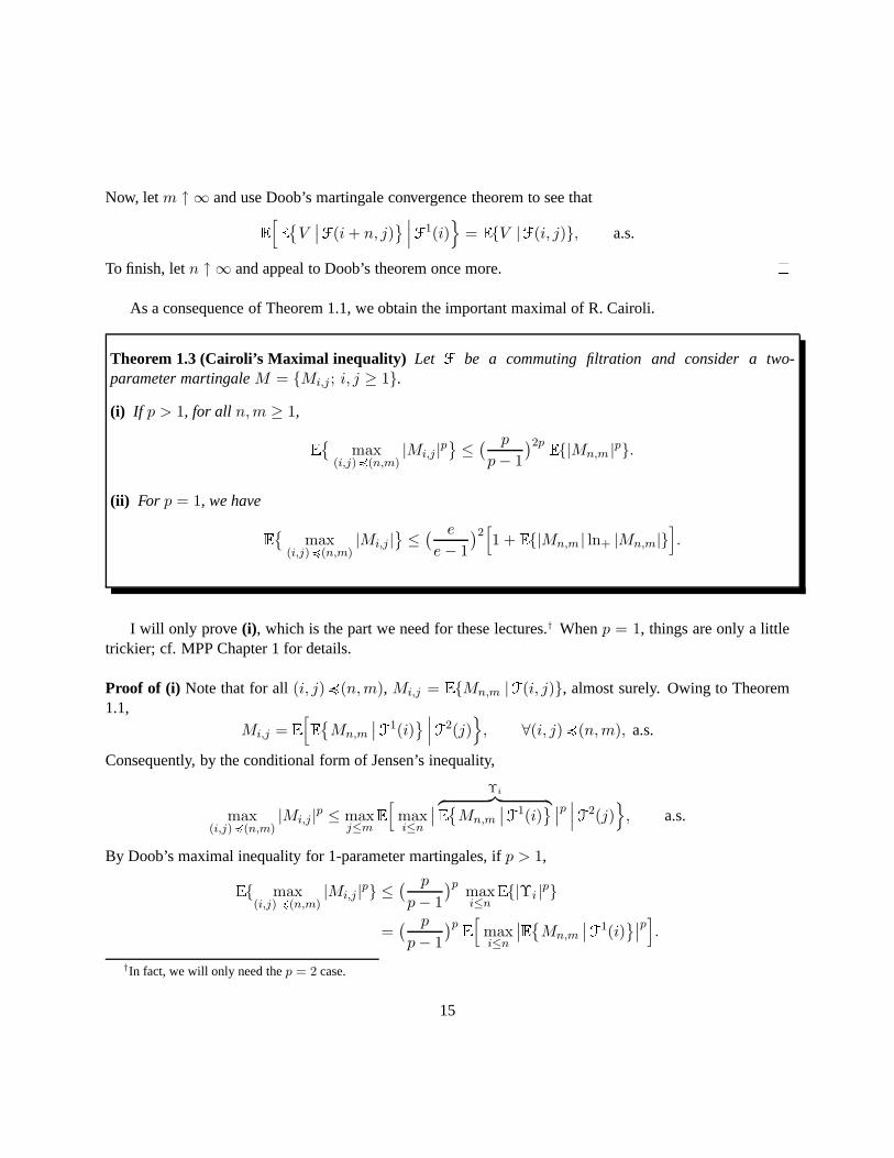
Now, letm ↑ ∞ and use Doob’s martingale convergence theorem to see that

E[E{V

∣∣F(i + n, j)} ∣∣∣F1(i)

}= E{V |F(i, j)}, a.s.

To finish, letn ↑ ∞ and appeal to Doob’s theorem once more. �

As a consequence of Theorem 1.1, we obtain the important maximal of R. Cairoli.

Theorem 1.3 (Cairoli’s Maximal inequality) Let F be a commuting filtration and consider a two-parameter martingaleM = {Mi,j ; i, j ≥ 1}.(i) If p > 1, for all n,m ≥ 1,

E{

max(i,j)4(n,m)

|Mi,j |p} ≤ ( p

p− 1)2p

E{|Mn,m |p}.

(ii) For p = 1, we have

E{

max(i,j)4(n,m)

|Mi,j |} ≤ ( e

e− 1)2

[1 + E{|Mn,m | ln+ |Mn,m|}

].

I will only prove (i), which is the part we need for these lectures.† Whenp = 1, things are only a littletrickier; cf. MPP Chapter 1 for details.

Proof of (i) Note that for all(i, j)4(n,m), Mi,j = E{Mn,m |F(i, j)}, almost surely. Owing to Theorem1.1,

Mi,j = E[E{Mn,m

∣∣F1(i)} ∣∣∣F2(j)

}, ∀(i, j)4(n,m), a.s.

Consequently, by the conditional form of Jensen’s inequality,

max(i,j)4(n,m)

|Mi,j |p ≤ maxj≤m

E[

maxi≤n

∣∣ Υi︷︸︸︷E{Mn,m

∣∣F1(i)} ∣∣p ∣∣∣F2(j)

}, a.s.

By Doob’s maximal inequality for 1-parameter martingales, ifp > 1,

E{ max(i,j) 4(n,m)

|Mi,j |p} ≤( p

p− 1)p max

i≤nE{|Υi |p}

=( p

p− 1)pE[

maxi≤n

∣∣E{Mn,m

∣∣F1(i)}∣∣p].

†In fact, we will only need thep = 2 case.

15

Apply Doob’s inequality again to finish. �

SOMETHING TO TRY: LetXi,j be i.i.d. random variables with mean0, and considerSn,m =∑∑

(i,j)4(n,m)

Xi,j .

Show thatS = {Sn,m; n,m ≥ 1} is a 2-parameter martingale with respect to a commuting filtration.

There is also a theory of2-parameter reversed martingales that can be used to prove the following in-triguing law of large numbers.

Theorem 1.4 (R. Smythe)Let Xi,j be i.i.d. random variables with meanµ, and consider the two-parameter random walkSn,m =

∑∑(i,j)4(n,m)

Xi,j . Then,

X1,1 ∈ L log L(P) =⇒ P{

limn,m→∞

Sn,m

nm= µ

}= 1, whereas

X1,1 6∈ L log L(P) =⇒ P{

lim supn,m→∞

|Sn,m|nm

= +∞}

= 1.

SOMETHING TO TRY: Check, using the Borel–Cantelli lemma, that

X1,1 6∈ L log L(P) ⇐⇒ P{

lim supn,m→∞

|Xn,m|nm

= +∞}

= 1.

Show that this implies the second half of Smythe’s theorem.

I will append Chapter 2 of MPP to illustrate two examples of martingale theory in classical analysis: oneto differentiation theory (the differentiation theorem of Lebesgue, as well as that of Jessen, Marcinkiewiczand Zygmund), and another to the the Haar function expansion of the elements ofL1([0, 1]N ).

16

Lecture 4

Capacity, Energy and Dimension

We now come to the second part of these lectures which has to do with “exceptional sets”. The most obviousclass of exceptional sets are those of measure0, where the measure is some nice one. As an example,consider a compact setE ⊂ Rd . One way to construct its Lebesgue measure is as follows: coverE by smallboxes, compute the volume of the cover, and then optimize over all the covers. That is,

|E| = limε→0+

inf{∑

i

[diam(Ei)]d : E1, E2, . . . closed boxes of diameter≤ ε with ∪i Ei ⊇ E}

.

Here, we are computing the diameter of the box as twice its`1-radius; i.e., it is the length of any side. Thisis equivalent to the usual definition of Lebesgue’s measure, although it is long out of fashion in standardanalysis courses.

1 Hausdorff Dimension and Measures

The first class of exceptional sets that we can discuss are those of Lebesgue’s measure0, of course. But,this is too crude for differentiating amongst very thin sets. For example, consider the rationalsQ , as well asCantor’s tertiary setC. While they are both measure0 sets,C is uncountable, whereasQ is not. We wouldlike a concrete way of saying thatC is larger thanQ , and perhaps measure how much larger, as well. Thereare many ways of doing this, and we will choose a route that is useful for our probabilistic needs. First,note that for anyα ≥ 0, we can define the analogue of|E| as above. Namely, define for any compact setE ⊂ Rd ,

Hα(E) = limε→0+

inf{ ∑

i

[diam(Ei)]α : E1, E2, . . . closed boxes of diameter≤ ε with ∪i Ei ⊇ E}

.

This makes sense even ifα ≤ 0.The set functionHα is called theα-dimensionalHausdorff measure. This terminology is motivated by

the following, which is proved by using the method given to us by Carath´eodory:

17

Theorem 1.1 The set functionHα is an outer measure on Borel subsets ofRd . For all α > d,Hα(E) = 0identically. On the other hand, whenα ≤ d is an integer,Hα(E) equals theα-dimensional Lebesgue’smeasure of Borel setE.

Remark For the above to hold, we have used`∞ balls (i.e., boxes). If you use2-balls in the definitioninstead, you will see that for integralα,Hα equalsωα timesα-dimensional Lebesgue’s measure, whereωα

is the volume of anα-dimensional ball of radius1. �

Hausdorff dimensions provide us with a more refined sense of how big a set is. Note that for any compact(or even Borel, say) setE, there isalwaysa critical α such that for allβ < α, Hβ(E) = 0, while for allβ > α,Hβ(E) = +∞. This is an easy calculation. But it leads to the following important measure-theoreticnotion of dimension:

dim(E) = inf{α : Hα(E) = 0} = sup{α : Hα(E) = +∞}.This is theHausdorff dimensionof E. If E ⊂ Rd is not compact, definedim(E) as supn≥1 dim(E ∩[−n, n]d).

How does one compute the Hausdorff dimension of a set? You typically proceed by establishing anupper bound, as well as a lower bound. The first step is not hard: just find a “good” coveringEi of diameterless thanε, and compute

∑i[diam(Ei)]α. Here is one way to get an upper bound systematically; other ways

abound.Suppose we are interested in computing the Hausdorff dimension of a given compact setE ⊂ [0, 1]d.

Fix a real numbern ≥ 1, and defineEj = [ jn , j+1

n [, for integers0 ≤ j ≤ n. Then, it is clear that thediameter of eachEj is no more than2n , while∪jEj ⊃ E. So,

Hα(E) ≤ ( 2n

)αNn(E),

whereNn(E) =∑

0≤j≤n 1{Ij,n ∩ E 6= ?} is the number of times the intervalsIj,n contains portions ofE. Therefore, if we can findα such thatlim supn n−αNn(E) < +∞, we havedim(E) ≤ α.† Incidentally,the minimalα such thatlim supn n−αNn(E) < +∞ is the so-calledupper Minkowski (or box) dimensionof E. If we write the latter asdim

M(E), we have shown that

dim(E) ≤ dimM

(E). (1.1)

If we replaceEj by ad-dimensional box of the form[ i1n , i1+1n [× · · · × [ idn , id+1

n [ and repeat the procedure,we obtain the upper Minkowski dimension ind dimensions, and Eq. (1.1) remains to hold.

†We do not requiren to be an integer here.

18

We now use this to obtain an upper bound for the tertiary Cantor setC. First, let us recall the followingiterative construction ofC: let C0 = [0, 1]. Now, remove the middle third to obtainC1 = [0, 1

3 ] ∪ [23 , 1].Next, remove the middle thirds of each of the two subintervals to getC2 = [0, 1

9 ]∪ [29 , 39 ]∪ [69 , 7

9 ]∪ [89 , 1], andso on. In this way, you have a decreasing sequence of compact subsets of[0, 1], and, as such,C = ∩nCn is anontrivial compact subset of[0, 1]. At thenth level of construction,Cn is comprised of2n intervals of length3−n. Therefore,|Cn| = (2

3 )n → |C| = 0. On the other hand, we just argued that there are2n boxes, ofdiameter no greater than (in fact, equal to)3n that coverC. Therefore, we have shown thatN3n(C) = 2n.In particular, for anyα > log3(2), lim supm→∞(3−m)−αN3m(E) = limm→∞ 3−mα2m = 0. So that,after a little work, we getdim

M(E) ≤ log3(2). In fact, it is easy to see, by the same reasoning, that

dimM (E) = log3(2). In any event, we obtain the following:

dim(C) ≤ log3(2) =ln 2ln 3

. (1.2)

We will show that this is sharp in that the above inequality is an equality. But first, a question:why notstick to Minkowski dimension?It is certainly easier to compute than Hausdorff dimension, and at first sight,more natural. To answer this, try computingdim

M(Q), or dim

Mof any other dense subset of[0, 1]d for that

matter! You will see that the answer is1! On the other hand, it is not hard to show thatdim(E) = 0 if E iscountable, for then we can writeE = {ri} and note that{ri} is a cover ofE with diameter less thanε. Thisseemingly technical difference is really a big one.

Now, to the lower bound fordim(C). Obtaining lower bound on Hausdorff dimension is, in principle,very hard, since you have to work uniformly over all covers. What makes things difficult is that there arealot of potential covers!

The ingenious idea behind obtaining lower bounds is due to O. Frostman who found it in his Ph.D. thesisin the 1935! Namely,

Theorem 1.2 (Frostman’s lemma)Suppose we knew that the compact setE carries a probability measureµ that is Holder-smooth in the following sense: there existsα > 0 and a constantC such that for allr ∈ (0, 1),

µ(B(y, r)) ≤ Crα,

for µ-almost ally, whereB(y, r) is the`∞-ball of radiusr abouty ∈ Rd . Then,dim(E) ≥ α.

There is a converse to this that we will only need once, and will not prove, as a result; for a proof, seeAppendix C of MPP.

19

Theorem 1.3 (Frostman’s Lemma (continued))Supposedim(E) ≥ α > 0. Then, for eachβ < α, thereexistsµ ∈ P(E) such that

supx∈Rd

supr∈(0,1)

µ{B(x, r)}rβ

< +∞.

Proof I will prove this when instead ofµ-almost allx, the lemma holds for allx. The necessary modifica-tions to prove the general case are technical but not hard.

Fix ε ∈ (0, 1), and consider any coverE1, E2, . . . of diameter≤ ε. Note that

1 = µ(E) ≤∑

i

µ(Ei) ≤ C∑

i

[diam(Ej)

]α.

Optimize over all such covers, and letε → 0, to see that1 ≤ 2CHα(E). The theorem follows, since thisshows that for anyβ < α,Hβ(E) = +∞. (To prove in the general case, note that ifµ(Ej) is not less thanC[diam(Ej)]α, we can coverEj by at most2d compact intervalsFj,1, . . . , Fj,2d of diameter less than twicethat ofEj , such thatµ(Fj,k) ≤ C[diam(Fj,k)]α ≤ 2αC[diam(Ej)]α. Thus,µ(Ej) ≤ 2α+dC[diam(Ej)]α,which is good enough.) �

We use this to complete our proof of the following.

Proposition 1.4 If C denotes the tertiary Cantor set,dim(C) = ln 2ln 3 .

Proof In light of what we have already done, we only need to verify the lower bound on dimension. Wedo this by finding a sufficiently smooth measure onC. Our choice is more or less obvious and is founditeratively as follows: construct the smoothest possible probability measureµn on Cn and “take limits”.Now, the smoothest and flattest probability measure onCn is the uniform measure,µn. It is easy to see thatfor all x ∈ [0, 1],

µn

([x− 3−n, x + 3−n]

) ≤ 2−n = (3−n)ln 2/ ln 3. (1.3)

This is suggestive, but we need to work a little bit more. To do so, we next note that theµn’s are nested:We write Cn = ∪2n

i=1Ii,n whereIi,n is an interval of length3−n. The nested property of theµn’s is thefollowing, which can be checked by induction:

∀n ≥ m,∀j = 1, . . . , 2m : µn(Ij,m) = µm(Ij,m) = 2−m.

20

Standard weak convergence theory guarantees us of the existence of a probability measureµ∞ on the com-pact setC such that for allm ≥ 1 and allj = 1, . . . , 2m,

µ∞(Ij,m) = µm(Ij,m) = 2−m.

Moreover, Eq. (1.3) extends toµ∞. Namely, for allx ∈ [0, 1] and alln ≥ 0,

µ∞([x− 3−n, x + 3−n]) ≤ (3−n)ln 2/ ln 3.

Now, if r ∈ (0, 1), we can findn ≥ 0 such that3−n−1 ≤ r ≤ 3−n. Therefore,

supx

µ∞([x− r, x + r]) ≤ supx

µ∞([x− 3−n, x + 3−n]) ≤ (3−n)ln 2/ ln 3 ≤ (3r)ln 2/ ln 3.

So, we have found a probability measureµ∞ on C, that satisfies the condition of Frostman’s lemma withC = 3ln 2/ ln 3 = 2 andα = ln 3/ ln 3. This completes our proof. �

2 Energy and Capacity

Supposeµ is a probability measure on some given compact setE ⊂ Rd . We will write this asµ ∈ P(E),and define for any measurable functionf : E × E → R+ ∪ {∞},

Ef (µ) =∫∫

f(x, y)µ(dx)µ(dx).

This is theenergyof µ with respect to the gauge functionf ; it is always defined although it may be infinite.The following energy forms are of use to us:

Energyα(µ) =∫∫

|x− y|−α µ(dx)µ(dy),

where|x| = max1≤j≤d |xj| for concreteness, although any other Euclidean norm will do just as well. Thisis the so-calledα-dimensionalBessel–Riesz energyof µ. The question, in the flavor of the previous section,is when does a setE carry a probability measure of finite energy?To facilitate the discussion, we define thecapacityof a setE by

Cf (E) =[

infµ∈P(E)

Ef (µ)]−1

, and in particular,

Capα(E) =[

infµ∈P(E)

Energyα(µ)]−1

.

The above is Gauss’ principle of minimum energy. Next, we argue that there is a minimum energy measurecalled the equilibrium measure. Moreover, its potential is essentially constant, and the constant is the energy.

21

Theorem 2.1 (Equilibrium Measure) SupposeE is a compact set inRd such that for someα > 0,Capα(E) > 0. Then, there existsµ ∈ P(E), such that

Energyα(µ) =[Capα(E)

]−1.

Moreover, forµ-almost allx, ∫|x− y|−α µ(dy) = Energyα(µ).

Proof By definition, there exists a sequence of probability measuresµn, all supported onE, such that (i)they have finite energy; and (ii) for alln ≥ 1, (1 + 1

n)[Capα(E)]−1 ≥ Energyα(µn) ≥ [Capα(E)]−1. Letµ be any subsequential limit of theµn’s. Sinceµ ∈ P(E) as well,Energyα(µ) ≥ [Capα(E)]−1. We aim toshow the converse holds too. By going to a subsequencen′ along whichµn′ converges weakly toµ, we seethat for anyr0 > 0,∫∫

|x−y|≥r0

|x− y|−α µ(dx)µ(dy) = limn′→∞

∫∫|x−y|≥r0

|x− y|−α µn′(dx)µn′(dy) ≤ [Capα(E)]−1.

Let r0 ↓ 0 and use the dominated convergence theorem to deduce the first assertion. For the second asser-tion, i.e., that the minimum energy principle is actually achieved for some probability measure.

Now, consider

Υη ={

x ∈ E :∫|x− y|−α µ(dy) < (1− η)Energyα(µ)

}, η ∈ (0, 1).

We wish to show thatµ(Υη) = 0 for all η ∈ (0, 1). If this is not the case for someη ∈ (0, 1), then, considerthe following

ζ(•) =µ(• ∩Υη)

µ(Υη).

Evidently,ζ ∈ P(E), and has finite energy. Define

λε = (1− ε)µ + εζ, ε ∈ (0, 1).

Then,λε is also a probability measure onE, and it, too, has finite energy. In fact, writingλε = µ−ε(µ−ζ),a little calculation shows that

Energyα(λε) = Energyα(µ) + ε2Energyα(µ− ζ)− 2ε∫∫

|x− y|−α µ(dx)[µ(dy)− ζ(dy)

].

(The energy ofµ− ζ is defined as ifµ− ζ were a positive measure.)

22

Sinceµ minimizes energy, the above is greater than or equal toEnergyα(µ). Thus,

ε2Energyα(µ− ζ) ≥ 2ε∫∫

|x− y|−α µ(dx)[µ(dy)− ζ(dy)

].

Divide by ε and letε → 0 to see that

Energyα(µ) ≤∫∫

|x− y|−α µ(dx) ζ(dy).

But by the definition ofΥη, the right hand side is no more than(1 − η)Energyα(µ), which contradicts theassumption thatµ(Υη) > 0. In other words,∫

|x− y|−α µ(dy) ≥ Energyα(µ), µ-a.s.

It suffices to show the converse inequality. But this is easy. Indeed, suppose

Gµ(x) =∫|x− y|−α µ(dy) ≥ (1 + η)Energyα(µ),

on a set of positiveµ-measure. The functionx 7→ Gµ(x) is theα-dimensional potentialof the measureµ.We could integrate [dµ] to get the desired contradiction, viz.,

Energyα(µ) =∫

Θη

Gµ(x)µ(dx) +∫

Θ{η

Gµ(x)µ(dx)

≥ (1 + η)Energyα(µ) · µ(Θη) +∫

Θ{η

Gµ(x)µ(dx),

whereΘη = {x : Gµ(x) ≥ (1 + η)Energyα(µ)}. Therefore, by Theorem 2.1 on equilibrium measure,

Energyα(µ) ≥ Energyα(µ)[(1 + η)µ(Θη) + µ(Θ{

η)]

= Energyα(µ)[1 + ηµ(Θ{

η)],

which is a contradiction, unlessµ(Θη) = 0. This concludes our proof. �

SOMETHING TO TRY: The α-dimensional Bessel–Riesz energy defines a Hilbertian pre-norm. Indeed,defineMα(E) to be the collection of all measures of finiteα-dimensional Bessel–Riesz energy onE. Onthis, define the inner product,

〈µ, ν〉 =∫∫

|x− y|−α µ(dx) ν(dy).

Check that this defines a positive-definite bilinear form onMα(E) if α ∈ (0, d). From this, conclude thatfor all µ, ν ∈Mα(E), 〈µ, ν〉2 ≤ Energyα(µ) · Energyα(ν). This fills a gap in the above proof.

23

Thecapacitary dimensionof a compact setE ⊂ Rd is defined as

dimc(E) = sup{α : Capα(E) > 0

}= inf

{α : Capα(E) = 0

}.

Theorem 2.2 (Frostman’s Theorem)Capacitary and Hausdorff dimensions are one and the same.

Proof Here is one half of the proof: we will show that if there existsα > 0 and a probability measureµ onE, such thatEnergyα(µ) < +∞ ⇒ dim(E) ≥ α. This shows thatdimc(E) ≤ dim(E), which is half thetheorem.

By Theorem 2.1, we can assume without loss of generality thatµ is an equilibrium measure. In particu-lar,

µ(B(x, r)) ≤ rα

∫|x− y|−α µ(dy) = rαEnergyα(µ),

µ-almost everywhere. Frostman’s lemma (Theorem 1.2) shows thatdim(E) ≥ α, as needed.For the other half, we envoke the second half of Frostman’s theorem (Theorem 1.3) to produce for each

β < dim(E) a probability measureµ ∈ P(E), such that

µ(B(x, r)) ≤ Crβ, ∀x ∈ Rd , r ∈ (0, 1).

But if D denotes the diameter ofE,

Energyγ(µ) =∞∑

j=0

∫∫2−j−1D≤|x−y|≤2−jD

|x− y|−γ µ(dx)µ(dy)

≤∞∑

j=0

2(j+1)γD−γ supx∈Rd

µ(B(x, 2−jD)

≤ C2γDβ−γ∞∑

j=0

2jγ2−jβ,

which sums ifγ < β. Thus, we have shown that for allγ < dim(E), Capγ(E) > 0, i.e.,dimc(E) ≥ γ forall γ < dim(E), which completes the proof. �

3 The Brownian Curve

Next, we roll up our sleeves and compute the Hausdorff dimension of a few assorted and interesting randomfractals that arise from Brownian considerations. Our goal is to illustrate the methods and ideas rather thanthe final word on this subject.

Throughout,B = {Bt; t ≥ 0} denotes Brownian motion inRd . Recall also thatB is a strong Markovprocess, and that

24

B hits points iffd = 1, i.e., ∃t > 0 : Bt = 0 ⇐⇒ d = 1.

In particular, note that whend = 1, the Brownian curve has full Lebesgue measure, and also full dimen-sion. On the other hand, whend ≥ 2, the Brownian curve has zero Lebesgue measure (L´evy’s theorem),despite the following result.

Theorem 3.1 If B denotesd-dimensional Brownian motion, whered ≥ 2, dim B(R+) = 2, a.s.

Proof We do this in two parts. First, we show thatdim B(R+) ≤ 2 (the upper bound), and then we showthatdim B(R+) ≥ 2 (the lower bound). In any event, recall thatd ≥ 2.

Proof of the upper boundRecall that for any intervalI ⊂ Rd ,

P{B[1, 2] ∩ I 6= ?} ≤ cκ(|I|), whereκ(ε) =

{εd−2, if d ≥ 3ln+

(1ε

), if d = 2

. (3.1)

We will obtain this sort of estimate, in the more interesting case of Brownian sheet, in the last lecture. Infact, one can show that the constantc depends only onM , as long asI ⊆ [−M,M ]d. ConsiderI1, . . . , Ind

cubes of side1n , such that (i)I◦i ∩ I◦j = ? if i 6= j; and (ii)∪nd

j=1Ij = [0, 1]d. Based on these, define

Ej =

{Ij , if Ij ∩B[1, 2] 6= ?

?, otherwise.

Note thatE1, . . . , End is a( 1n)-cover ofB[1, 2] ∩ [0, 1]d. Thus,

Hα

(B[1, 2] ∩ [0, 1]d

) ≤ lim infn→∞

nd∑j=1

n−α1{Ij∩B[1,2] 6=?}.

Consequently, as long asα > 2,

E{Hα

(B[1, 2] ∩ [0, 1]d

)} ≤ c lim infn→∞

nd∑j=1

n−ακ(

1n

)= c lim inf

n→∞ nd−ακ(

1n

)= 0.

In particular,dim(B[1, 2]∩ [0, 1]d) ≤ 2, a.s. Similarly,dim(B[a, b]∩ [−n, n]d) ≤ 2, a.s. for any0 < a < bandn > 0. Let n ↑ ∞, a ↓ 0 andb ↑ ∞, all along rational sequences to deduce thatdim B(R+) ≤ 2,a.s. This uses the easily verified fact that wheneverA1 ⊆ A2 ⊆ · · · are compact, and ifHα(Aj) = 0, thenHα(∪jAj) = 0.

25

Proof of the lower boundFor the converse, we will show thatdim B[1, 2] ≥ 2, and do this by appealing toFrostman’s theorem (Theorem 2.2). To do so, we need to define a probability, or at least a finite, measure onthe Brownian curve. The most natural measure that lives on the curve of{Bs; 1 ≤ s ≤ 2} is the occupationmeasure:

O(E) =∫ 2

11{Bs∈E} ds.

With this in mind, note that for anyα > 0,

Energyα(O ) =∫∫

|x− y|−α O (dx)O (dy) =∫ 2

1

∫ 2

1|Bs −Bt|−α ds dt.

By Frostman’s theorem, it suffices to show thatE{Energyα(O )} < +∞ for all 0 < α < 2. But this is easy.Indeed, note that

E{Energyα(O )

}= 2

∫ 2

1

∫ 2

sE{|Bt−s|−α} ds dt = 2

∫ 2

1

∫ 2

s|t− s|−α

2 ds dt× E{|Z|−α},

whereZ is ad-dimensional vector of i.i.d. standard normals. Sinceα < 2, the double integral is finite. Itsuffices to show thatE{|Z|−α 〉 < +∞. But

E{|Z|−α} =∫ ∞

0P{|Z|−α > λ} dλ

≤ 1 +∫ ∞

1P{|Z|−α > λ} dλ

= 1 + α

∫ 1

0P{|Z| < u}u−α−1 du (u = λ−

1α )

= 1 + α

∫ 1

0

[P{|Z1| ≤ u}]d

u−α−1 du.

But P{|Z1| ≤ u} = (2π)−12

∫ u−u e−

12λ2

dλ ≤ u. Hence, usingd ≥ 2 > α,

E{|Z|−α} ≤ 1 + α

∫ 1

0ud−α−1 du =

d

d− α< +∞,

as promised. �

Here is a slick proof of L´evy’s theorem alluded to earlier.

Theorem 3.2 (P. Levy) If B is Brownian motion inRd and ifd ≥ 2, B(R+) has zero Lebesgue’s measure,a.s.

26

Proof I will prove this whend ≥ 3 where things are alot simpler, and appeal to an argument that, in physicsliterature, is calledgroup renormalization. Tacitly held, throughout, is the fact thatE{λd (B(0, t))} < ∞;this is a ready consequence of the easy estimateE{sup0≤s≤t |Bs|d} < +∞.

If λd denotes Lebesgue’s measure onRd , note that

E{λd (B(0, 2))} ≤ E{λd(B(0, 1))} + E{λd (B(1, 2))}.We make two observations:(i) E{λd(B(1, 2))} = E{λd (B(0, 1))}; and (ii) by Brownian scaling,

E{λd (B(0, 2))} = E{λd (√

2B(0, 1))} = 2d2 E{λd (B(0, 1))}, thanks to the scaling properties ofλd.

Combining these observations, we get2d2 E{λd (B(0, 1))} ≤ 2E{λd (B(0, 1))}, which is impossible un-

lessE{λd (B(0, 1))} = 0, sinced ≥ 3.

��

��A few words about thed = 2 case: Levy’s theorem is harder to prove whend = 2, and uses the estimate

(3.1) and a covering argument. �

4 Brownian Motion and Newtonian Capacity

We now look at an elementary connection between three-dimensional Brownian motion and Newtoniancapacity. LetB = {Bt; t ≥ 0} denote three-dimensional Brownian motion, and consider the linear operator

Uf(x) = E{ ∫ ∞

0f(Bs + x) ds

}.

Here,x ∈ R3 andf : R3 → R+ is measurable. We can easily evaluate this as follows. A few liberal dosesof Fubini-Tonelli yield:

Uf(x) =∫ ∞

0

∫R3

f(x + z)e−

‖z‖22s

(2πs)32

dz ds

=14π

∫R3

‖x− y‖−1f(y) dy.

Now, supposef is a probability density function on some (say, nice compact) setE ⊂ R3 . Then,Uf(x) isthe expected amount of time spent inE, weighed according tof , and starting atx ∈ R3 . Now, suppose theBrownian motion itself starts according to the pdff . Then, this expected time is∫

R3

Uf(x)f(x) dx =14π

∫R3

∫R3

‖x− y‖−1f(y) dy f(x) dx.

You should recognize the right hand side as(4π)−1 times the Newtonian energy of the measuref(x) dx.In summary, if we start Brownian motion inE according tof , the expected amount of time spent inE,

27

weighed accroding tof , if precisely 14π Energy1(f), wheref(x) is identified with the measuref(x)dx here.

SOMETHING TO TRY: Check that wheneverB is Brownian motion inRd (d ≥ 3) that starts according tosome pdff , ∫

Rd

E{ ∫ ∞

0f(Bs + x) ds

}f(x) dx = cEnergyd−2(f),

and computec. Why does this fail whend = 2 or d = 1?

5 Riesz Transforms andHHHp Spaces

Below, if will prove that ifα ∈ (0, d), the Fourier transform of the functionRd 3 ξ 7→ ‖ξ‖−α is a constantmultiple of‖ξ‖−(d−α). We will compute this constant also. However, let us see what this implies for energy.Recall that

Energyα(µ) =∫Rd

Rµ(x)µ(dx),

whereRµ(x) =∫Rd |x− y|−α µ(dy). We are only interested in whether or not the above is finite for some

measureµ. Thus, we cheat at the last moment and replace the`∞ norm by`2 norm to getEnergyα(µ) =∫Rd Rµ(x)µ(dx), where

Rµ(x) =∫Rd

‖x− y‖−α µ(dy)

is the so-calledα-dimensionalRiesz transformof µ. Using obviousL2 notation,Energyα(µ) = (Rµ, µ).Having noted theL2 connection, we apply Fourier transforms (via Plancherel) to see that

Energyα(µ) = (2π)−d(Rµ, µ).

But,R is a convolution operator that can be identified with the kernelR(a) = ‖a‖−α. Therefore,Rµ = Rµ.On the other hand, we just mentioned that the Fourier transform ofR is c‖ξ‖−(d−α), wherec = Cα fromLemma 5.1 below. Thus, whenα ∈ (0, d),

Energyα(µ) = (2π)−dc

∫Rd

‖ξ‖−(d−α)|µ(ξ)|2 dξ.

Thus,Energyα(µ) is equivalent (i.e., converges iff the following does) to theHd−α2

-norm:

‖µ‖2d−α

2

=∫Rd

∣∣µ(ξ)∣∣2{1 + ‖ξ‖2

}−d−α2 dξ.

Thus we have linked the computations of the lecture of D. BLOUNT earlier this week to energy computa-tions (in his notation,γ = −1

2(d − α).) If you want to have a more in-depth look at connections to energy

28

and dimension, try the following.

SOMETHING TO TRY: Let X = {Xt; t ≥ 0} be an isotropic L´evy process inRd . That is, a process withi.i.d. increments whose characteristic function is given byE{eiξ·Xt} = exp{− t

2‖ξ‖α}. It is known thatα ∈ (0, 2] is necessary. Whenα = 2, X is just Brownian motion.

Suppose further thatα ∈ (0, d), and define the weighted occupation measure

O (E) =∫ ∞

01E(Xs)e−s ds.

(i) Check that its Fourier transform isO (ξ) =∫∞0 eiξ·Xse−s ds.

(ii) Use the above to show thatE{|O (ξ)|2} ={

12‖ξ‖α + 1

}−1. In particular, for anyβ ∈ (0, d),

E{Energyβ(O )

}= (2π)−dc

∫Rd

‖ξ‖−(d−β){

12‖ξ‖α + 1

}−1dξ.

(iii) Conclude that wheneverβ < α, Energyβ(O ) < +∞, a.s.

(iv) Use Frostman’s theorem to show that, with probability one,dim(X(R+)) ≥ α. One can show thatthis is sharp. That is, whenα ∈ (0, d), dim(X(R+ )) = α, a.s. Whenα = 2, we did this last partexplicitly in Theorem 3.1. Here, the strategy is the same, but we need hitting probability estimates forstable processes.

Let me conclude with the following promised calculation, then. Henceforth, for anyγ > 0,

Ψγ(ξ) = ‖ξ‖−γ .

Lemma 5.1 For anyγ ∈ (0, d), Ψγ = 1Cγ

Ψd−γ , whereCγ = 2−γ2 π−d

2 Γ(d−γ2 )/Γ(γ

2 ).

Proof We will relate the mention Fourier transform to the Laplace transform of a Gaussian, first. This mayseem like magic, but if you apply some more Fourier analysis (namely, Bochner’s subordination), you canexplain this more clearly; cf. MPP for the latter.

Note that forθ > 0 andβ > −1,∫∞0 e−tθtβ dt = θ−(1+β)Γ(1 + β). In particular,∫ ∞

0e−t‖ξ‖2tβ dt = ‖ξ‖−(2+2β)Γ(1 + β).

29

Now, take a well-tempered functionϕ and consider∫Rd

ϕ(ξ)‖ξ‖−(2+2β) dξ =1

Γ(1 + β)

∫ ∞

0tβ

( ∫Rd

ϕ(ξ)e−t‖ξ‖2 dξ)

dt.

(In truth, theϕ should be a tempered distribution.) Apply Parseval’s identity:(ϕ, f) = (2π)−d(ϕ, f) todeduce∫Rd

ϕ(ξ)‖ξ‖−(2+2β) dξ =(2π)d

Γ(1 + β)

∫ ∞

0tβ

( ∫Rd

ϕ(ξ)e−‖ξ‖2/2t

(2πt)d2

dξ)

dt

=(2π)d

Γ(1 + β)

∫Rd

ϕ(ξ)( ∫ ∞

0

e−‖ξ‖2/2t

(2πt)d2

tβ dt)

dξ (s = ‖ξ‖22t )

=(2π)d

Γ(1 + β)(2π)−

d2 2

d2−β−1Γ(d

2 − β − 1)∫Rd

ϕ(ξ)‖ξ‖d−(2β+2) dξ.

Let 2β + 2 = γ to finish. �

30

Lecture 5

Brownian Sheet, Potential Theory, andKahane’s Problem

Recall that a Brownian sheetB = {B(s, t); s, t ≥ 0} is just a real process defined as

B(s, t) = W ([0, s] × [0, t]), ∀s, t ≥ 0,

whereW denotes white noise onR2 . We will refer to this asone-dimensional Brownian sheetto stress thatthe process takes its values inR.

By ad-dimensional Brownian sheet, we mean thed-dimensional processB = {B(s, t); s, t ≥ 0} suchthatB1, B2, . . . , Bd are i.i.d. (1-dimensional) Brownian sheets. Of course,Bi = {Bi(s, t); s, t ≥ 0}.

1 Polar Sets

The following theorem, due to S. Kakutani, is the cornerstone of probabilistic potential theory.

Theorem 1.1 (S. Kakutani) Let b denoted-dimensional Brownian motion, and consider a fixed compactE ⊂ Rd . Then,

P{∃t > 0 : bt ∈ E} > 0 ⇐⇒ Capd−2(E) > 0.

The above relatesE to what is called apolar set. Probabilistically, a setE is polar for a processX = {Xt; t ∈ T} if with positive probability,∃t ∈ T : Xt ∈ E. Thus, Kakutani’s theorem characterizespolar sets for Brownian motion. This notion of polarity matches with the one from harmonic analysis, whichhas to do with the removable singularities of the Dirichlet problem off the set. Amongst other things, fairlyroutine calculations show that theα-dimensional capacity of a ball of radiusε is of orderεα if α > 0, and[log(1/ε)]−1 if α = 0. That is, Theorem 1.1 contains the hitting probability estimate (3.1) of Lecture 4.

31

A more recent result, this time for the sheet is,

Theorem 1.2 (D. Kh. and Z. Shi) If E is a compact set inRd , P{B(R2+)∩E 6= ?} > 0 iff Capd−4(E) >

0. In fact, for anyM > 0, there existsc1 andc2, such that for all compactE ⊂ [−M,M ]d,

c1Capd−4(E) ≤ P{B[1, 2]2 ∩ E 6= ?} ≤ c2Capd−4(E).

We will prove this shortly. However, let me mention a variant: supposeX1, . . . ,XN are i.i.d. isotropicstable processes inRd all with indexα ∈ (0, 2]. This means that eachX` is anRd -valued Levy process withcharacteristic function

E{eiξ·X` (t)} = exp(− 1

2‖ξ‖α), ∀ξ ∈ Rd , t ≥ 0, ` = 1, . . . , d.

The 12 is to ensure that whenα = 2, X` is standard Brownian motion. Theα-dimensional,N -parameter

additive stable processis the random field

X(t) = X1(t1) + · · · + XN (tN ), ∀t ∈ RN+ .

Theorem 1.3 (F. Hirsch and S. Song; MPP Ch. 11)If X is anN -parameter,d-dimensional additive sta-ble process of indexα, and ifE ⊂ Rd is a given compact set, thenE is polar forX iff Capd−αN (E) > 0.

The above, together with the energy/covering arguments of Lecture 4 (cf. Theorem 3.1 there), this shows

Theorem 1.4 If X is anN -parameter,d-dimensional additive stable process of indexα,

dim(X(RN+ )) = αN ∧ d, a.s.

The above two theorems provide us with processes that correspond to arbitrary dimensions and capaci-ties.

2 Application to Stochastic Codimension

The preceeding has a remarkable consequence about a large class of random sets. We say that a ran-dom setX ⊂ Rd hascodimensionβ, if β is the critical number such that for all compact setsE ⊂ Rd

32

with dim(E) > β, P{X ∩ E 6= ?} > 0, while for all compact setsF ⊂ Rd with dim(F ) < β,P{X ∩ F 6= ?} = 0. The notion of codimension was coined in this way in Kh-Shi ’99, but the essen-tial idea has been around in the works of Taylor ’65, Lyons ’99, Peres ’95,· · ·

When it does exist, the codimension of a random set is a nonrandom number.

Warning: Not all random sets have a codimension.

As examples of random sets thatdo have codimension, we mention the following consequence of The-orem 1.3:

Corollary 2.1 If Z denotes an(N, d)-additive stable process of indexα ∈ (0, 2], codim(Z[1, 2]N ) =d− αN.

We now wish to use Theorem 1.3 to prove the following result. In the present form, it is from MPP Ch.11, but ford = 1, it is from Kh-Shi ’99.

Theorem 2.2 (MPP Ch. 11) If X is a random set inRd that has codimensionβ ∈ (0, d),

dim(X) = d− codim(X), a.s.

That is, in the best of circumstances,

��

��dim(X) + codim(X) = topological dimension.

A note of warning: ifX is not compact,dim(X) can be defined bysupn≥1 dim(X ∩ [−n, n]d).

The proof depends on the following result that can be found in the works of Yuval Peres ’95, but withpercolation proofs.

Lemma 2.3 (Peres’ lemma)For eachβ ∈ (0, d), there exists a random setΛβ , whose codimension isβ.Moreover,dim(Λβ) = d− β, almost surely.

33

Proof Let Λβ = Z(RN+ ), whereZ is an(N, d)-addtive stable process. The result follows from Corollary

2.1 and Theorem 1.4. �

Proof of Theorem 2.2By localization, we may assume thatX is a.s. compact. LetΛβ = ∪∞i=1Λiβ, where

Λ1β,Λ2

β , . . . are iid copies of the sets in Peres’ lemma, and are all totally independent of our random setX.Then, by Peres’ lemma and by the lemma of Borel–Cantelli,

P{Λβ ∩X 6= ? |X} =

{0, on{dim(X) < β}1, on{dim(X) > β} .

On the other hand, by the very definition of codimension,

P{Λβ ∩X 6= ? |Λβ} =

{0, if codim(X) > d− β = dim(Λβ)> 0, if codim(X) < d− β

.

Take expectations of the last two displays to see that for anyβ ∈ (0, d),

codim(X) < d− β =⇒ dim(X) ≥ β, a.s.

codim(X) > d− β =⇒ dim(X) ≤ β, a.s.

This easily proves our theorem. �

3 Proof of Theorem 1.2

We begin with an elementary, though extremely useful, lemma.

Lemma 3.1 (R. E. A. C. Paley and A. Zygmund)If Z ≥ 0 a.s., and ifZ ∈ L2(P),

P{Z > 0} ≥ |E{Z}|2E{Z2} ,

where0÷ 0 = 0.

Proof By the Cauchy–Schwarz inequality,

E{Z} = E{Z; Z > 0}≤

√E{Z2}P{Z > 0}.

34

Square and solve. �

Roughly speaking, the strategy of proof of Theorem 1.2 is to show thatB[1, 2]2 intersectsE iff theoccupation measure evaluated at somef ∈ P(E) is large, wheref ∈ P(E) means thatf is a probabilitydensity function supported onE, where the latter is given by

O (f) =∫

[1,2]2f(B(s, t)) ds dt.

Lemma 3.2 For eachM > 0, there exists a constantc = c(M) > 1 such that for all pdf’sf on [−M,M ]d,

E{O (f)} ≥ c.

Proof The law of the variateB(s, t) is√

stZ, whereZ = (Z1, . . . , Zd) is a vector of i.i.d. standard nor-mals. The lemma follows from direct compmutations, since this pdf is easily seen to be bounded below on[−M,M ]d. �

Lemma 3.3 For eachM > 0, there exists a constantc = c(M) > 1 such that for all pdf’sf on [−M,M ]d,

E{∣∣O(f)

∣∣2} ≤ cEnergyd−4(f).

To develop Kakutani’s theorem by the methods of this lecture, start with

SOMETHING TO TRY: Let b = {bt; t ≥ 0} denoted-dimensional Brownian motion. Then, show that foreachM > 0, there exists a constantc = c(M) > 1 such that for all pdf’sf on [−M,M ]d,

E{∣∣∣ ∫ 2

1f(bs) ds

∣∣∣2} ≤ cEnergyd−2(f).

Also show that there existsc = c(M) > 0, such that for all pdf’sf on [−M,M ]d,

E{ ∫ 2

1f(bs) ds

}≥ c.

35

Proof of Lemma 3.3Note that

E{∣∣O (f)

∣∣2} = E{ ∫

[1,2]2

∫[1,2]2

f(B(s))f(B(t)) ds dt}

= E{ ∫

[1,2]2

∫[1,2]2

f(B(s f t) + ξ1

)f(B(sf t) + ξ1

)ds dt

}

where

ξ1 = B(s)−B(s f t), and

ξ2 = B(t)−B(sf t).

Note that(i) ξ1 and ξ2 are independent; and(ii) the pdf of B(s f t) is bounded above by a constant,uniformly for all s, t ∈ [1, 2]2. Indeed, the latter pdf, atx ∈ Rd , is

(2π)−d2 (s1 ∧ t1)−

d2 (s2 ∧ t2)−

d2 exp

(− ‖x‖2

2(s1 ∧ t1)(s2 ∧ t2)

)≤ 1.

Thus,

E{∣∣O (f)

∣∣2} ≤ E{ ∫

[1,2]2

∫[1,2]2

∫Rd

f(x + ξ1)f(x + ξ2) dx ds dt}

= E{ ∫

[1,2]2

∫[1,2]2

∫Rd

f(x)f(x + ξ2 − ξ1) dx ds dt}

= E{ ∫

[1,2]2

∫[1,2]2

∫Rd

f(x)f(x + B(t)−B(s)

)dx ds dt

}.

Now, we proceed to a variance estimate as we did in Lemma 2.2 of Lecture 2 ford = 1. Indeed, the varianceof each of the coordinates ofB(t)−B(s) is bounded above and below by constant multiples of|t−s|. Thisleads to

E{∣∣O (f)

∣∣2} ≤ c

∫[1,2]2

∫[1,2]2

∫Rd

∫Rd

f(x)f(x + y)e− |y|2

c|t−s|

|t − s| d2dx dy ds dt

= cEnergyd−4(f),

after a few more lines of calculations. �

Proof of Theorem 1.2: Lower BoundIf there are pdf’s supported byE, choosef to be any one of themand note that

O (f) > 0 =⇒ B[1, 2]2 ∩ E 6= ?.

36

So, combine this with Lemmas 3.2 and 3.3 to get

P{B[1, 2]2 ∩ E 6= ?} ≥ P{O (f) > 0}

≥ |E{O (f)}|2E{|O (f)|2}

≥ c[Energyd−4(f)

]−1.

We have used the Paley–Zygmund inequality in the second-to-last line; cf. Lemma 3.1. This holds uniformlyover all pdf’sf onE. ReplaceE by its closeε-enlargementEε, we get

P{B[1, 2]2 ∩ Eε 6= ?} ≥ c[

infµ∈P(Eε):

µ=absolutely continuous

Energyd−4(µ)]−1

.

Any µ ∈ P(E) can be approximated, in the sense of weak convergence, by absolutely continuousµε ∈P(Eε). A little Fourier analysis, then, shows that asε → 0, Energyα(µ) is approximable byEnergyα(µε);cf. the last section of Lecture 4 for the requisite material on Fourier analysis. On the other hand,P{B[1, 2]2∩Eε 6= ?} → P{B[1, 2]2 ∩E 6= ?}, asε → 0. This yields,

P{B[1, 2]2 ∩ E 6= ?} ≥ c[

infµ∈P(E)

Energyd−4(µ)]−1

,

which equalscCapd−4(E). �

We now turn to the more difficult

Proof of Theorem 1.2: Upper Bound (sketch)Define the 2-parameter martingaleMf by

Mf(t) = E{O (f) |F(t)},wheref is a pdf onEε, andF is the natural 2-parameter filtration ofB. Clearly, for anys ∈ [1, 3

2 ]2,

Mf(s) =∫

[1,2]2E{f(B(t))

∣∣F(s)}

dt

≥∫

t< s:t∈[1,2]N

E{f(B(t))

∣∣F(s)}

dt

=∫

t< s:t∈[1,2]N

E{f(B(t)−B(s) + B(s)

) ∣∣F(s)}

dt.

Now, recall that whenevert< s, B(t) − B(s) is independent ofF(s), and whose coordinatewise varianceis, upto a constant,|t− s|. A few more lines show that for anys ∈ [1, 3

2 ]2,

Mf(s) ≥ cGf(B(s)

),

37

whereGµ(x) =∫Rd |x−y|−d+4 µ(dy) if d > 4,Gµ(x) =

∫Rd log+( 1

|x−y|)µ(dy), if d = 4, andGµ(x) = 1,

if d < 4. Let T be any measurable variate in[1, 32 ]2 ∪ {∞}, such thatT 6= ∞ iff ∃s ∈ [1, 3

2 ]2 such thatB(s) ∈ E, and in which case,B(T) ∈ E. Then, ignoring null sets, we have

sups∈[1,

32 ]2

Mf(T) ≥ cGf(B(T)

) · 1{T 6=∞}.

Square both sides, and take expectations:

E{

sups∈[1,

32 ]2

∣∣Mf(T)∣∣2} ≥ cE

{∣∣Gf(B(T)

)∣∣2 · 1{T 6=∞}}.

Now, if P{T 6= ∞} = 0, there is nothing to prove. Else, chooseµ(•) = P{B(T) ∈ • |T 6= ∞}(µ ∈ P(E)), to see that

E{

sups∈[1,

32 ]2

∣∣Mf(T)∣∣2} ≥ cE

{∣∣Gf(B(T)

)∣∣2 ∣∣T 6= ∞}× P{T 6= ∞}

≥ c∣∣∣E{Gf

(B(T)

) ∣∣T 6= ∞}∣∣∣2 × P{T 6= ∞}

= c∣∣∣ ∫

Gf(x)µ(dx)∣∣∣2 × P{T 6= ∞}.

On the other hand, by Cairoli’s inequality, the left hand side is bounded above by16E{|O (f)|2} ≤c′Energyd−4(f), thanks to Lemma 3.3. Combining things, we have, for this specialµ ∈ P(E),

cEnergyd−4(f) ≥∣∣∣ ∫ Gf(x)µ(dx)

∣∣∣2 × P{B[1, 32 ]2 ∩ E 6= ?}.

This holds for any pdff . Now, choose pdf’sf that converge weakly toµ. A little Fourier analysis showsthat we can do this so that the energies of thef ’s also approximate that ofµ, and

∫Gf(x)µ(dx) '∫

Gµ(x)µ(dx) = Energyd−4(µ). This completes our proof. �

SOMETHING TO TRY: Try and mimick the above sketched proof to show the upper bound in Kakutani’stheorem. You may ignore the Fourier analysis details.

4 Kahane’s Problem

We come to the last portion of these lectures, which is on a class of problems that I call Kahane’s problem,due to the work of J.-P. Kahane in this area.

38

Kahane’s problem for a random fieldX is: “when doesX(E) have positive Lebesgue’s measure?” Iwill work the details out for Brownian motion, where things are easier. The problem for the Brownian sheetwas partly solved by Kahane (cf. his ’86 book) and completely solved by Kh. ’99 in caseN = 2. Recentwork of Kh. and Xiao ’01 has completed the solution to Kahane’s problem and a class of related problems,and we hope to write this up at some point. Here is the story for Brownian motion, where we work thingsout more or less completely. The story for Brownian sheet is more difficult, and I will say some words aboutthe details later.

Theorem 4.1 (Kahane; Hawkes)If B denotes Brownian motion inR, and ifE ⊂ R+ is compact, then

E{|B(E)|} > 0 ⇐⇒ Cap 12(E) > 0.

In particular,

dim(E) > 12 =⇒ |B(E)| > 0, with positive probability

dim(E) < 12 =⇒ |B(E)| = 0, a.s.

You can interpret this as a statement about hitting proabilities for the level sets of Brownian motion, viz.,∫Rd

P{B−1{a} ∩E 6= ?} da > 0 ⇐⇒ Cap 12(E) > 0.

I will prove the following for Brownian motion. It clearly implies the above theorem upon integration.

Theorem 4.2 SupposeE ⊂ [1, 2] is compact, and fixM > 0. Then, there existsc1 andc2 such that for all|a| ≤ M ,

c1Cap 12(E) ≤ P{a ∈ B(E)} ≤ c2Cap1

2(E).

As a simple consequence of this and Frostman’s theorem, we see that the critical dimension forB−1{0}to hit a set is1

2 . Equivalently, the zero set,B−1{0}, has codimension12 . Since the topological dimension ofB−1{0} is 1, by Theorem 2.2,

Corollary 4.3 (P. Levy) With probability one,dim B−1{0} = 12 .

39

Proof Without loss of any generality, we may and will assume thatE ⊆ [0, 1].For anyµ ∈ P(E) and for alla ∈ R, define

Jaε (µ) = (2ε)−1

∫ ∞

01{|Bs−a|≤ε} µ(ds).

Then, for everyM > 0, there existsc such that

infε∈(0,1)

infa∈[−M,M ]

E{Jaε (µ)} ≥ c, and

supa∈R

supε∈(0,1)

E{|Jaε (µ)|2} ≤ Energy 1

2(µ).

(4.1)

Now, we apply Paley–Zygmund inequality:

P{a ∈ B(E)} ≥ P{Jaε (µ) > 0}

≥ |E{Jaε (µ)}|2

E{|Jaε (µ)|2}

≥ c

Energy 12(µ)

.

Since this holds for allµ ∈ P(E), we obtain the desired lower bound.Let {Ft}t≥0 denote the filtration ofB and consider the martingale

Ma,εt (µ) = E{Ja

ε (µ) |Ft}, ∀t ≥ 0.

Clearly,

Ma,εt (µ) ≥ (2ε)−1

∫s≥t

P{|Bs − a| ≤ ε |Ft}µ(ds) · 1{|Bt−a|≤ ε2}

≥ (2ε)−1

∫s≥t

P{|Bs−t| ≤ 12ε}µ(ds) · 1{|Bt−a|≤ ε

2}

≥ cε−1

∫s≥t

( ε√s− t

∧ 1)

µ(ds) · 1{|Bt−a|≤ ε2}

Let σε = inf{s ∈ E : |Bs − a| ≤ 12ε}. This is a stopping time and on{σε < ∞},

Ma,εσε

(µ) ≥ cε−1

∫s≥σε

[ ε√s− σε

∧ 1]µ(ds),

since all bounded Brownian martingales are continuous. Now, we chooseµ carefully: WLOGP{σε <∞} > 0 which implies thatµε ∈ P(E), where

µε(•) = P{σε ∈ • |σε < ∞}.

40

Thus, by the optional stopping theorem,

1 ≥ E{Ma,εσε

(µε);σε < ∞}≥ cε−1

∫∫s≥t

( ε√s− t

∧ 1)

µε(ds)µε(dt) · P{σε < ∞}

≥ c

2ε−1

∫∫ ( ε√s− t

∧ 1)

µε(ds)µε(dt) · P{σε < ∞}

=c

2

∫∫ ( 1√s− t

∧ 1ε

)µε(ds)µε(dt) · P{σε < ∞}.

Fix δ0 > 0 and from the above deduce that for allε small,

1 ≥ c

2

∫∫|s−t|≥δ0

|s− t|− 12 µε(ds)µε(dt) · P{ inf

t∈E|Bt − s| ≤ 1

2ε}.

Let ε → 0, and envoke Prohorov’s theorem to getµ ∈ P(E) such that

P{a ∈ B(E)} ≤ 2c

[ ∫∫|s−t|≥δ0

|s− t|− 12 µ(ds)µ(dt)

]−1.

Let δ0 ↓ 0 to finish. �

To prove the general result for a Brownian sheet, one needs the properties of the processB around atime pointt. There are2N different notions of ‘around’, one for each quadrant centered att, and this leads to2N differentN -parameter martingales, each of which is a martingale with respect to a commuting filtration,but each filtration is indeed a filtration with respect to a different partial order. The details are complicatedenough forN = 2 and can be found in my paper in theTransactions of the AMS(1999). WhenN > 2, thedetails are more complicated still and will be written up in the future. The end result is the following:

Theorem 4.4 (Kh and Xiao ’01) If B denotes(N, d) Brownian sheet andE ⊂ RN+ is compact,

E{|B(E)|} > 0 ⇐⇒ Cap d2(E) > 0.

To recapitulate the picture we have, by Theorem 1.2, whend ≥ 2N , E{|B(RN+ )|} = 0. Thus, the above

addresses portions of the range in the remaining low-dimensional cased < 2N . A consequence of thisdevelopment is that

dim(E) > d2 =⇒ |B(E)| > 0, with positive probability

dim(E) < d2 =⇒ |B(E)| = 0, a.s.

41

I will end with a related

CONJECTURE: SupposeX is an(N, d) symmetric stable sheet with indexα ∈ (0, 2) (see below.) Then, forany compactE ⊂ RN

+ , E{|X(E)|} > 0 iff Cap dα(E) > 0.

At the moment, this seems entirely out of the reach of the existing theory, but the analogous result foradditive stable processes, and much more, holds (joint work with Xiao–will write up later.)

To finish: {Xt; t ∈ RN+ } is an(N, d) symmetric stable sheet if it has i.i.d. cooridinates and the first

coordinate has the representationX1t =

∫1{04 s4 t}X(ds), whereX is a totally scattered random measure

such that for every nonrandom measurableA ⊂ RN+ , E{exp[iξX(A)]} = exp(−1

2 |A| ‖ξ‖α). (Scatteredmeans that for nonrandom measurableA andA′ in RN

+ , if A ∩A′ = ?, X(A) andX(A′) are independent.)

42

Bibliography

Adler, R. J. (1977). Hausdorff dimension and Gaussian fields.Ann. Probability 5(1), 145–151.

Adler, R. J. (1980). A Hölder condition for the local time of the Brownian sheet.Indiana Univ. Math. J. 29(5),793–798.

Adler, R. J. (1981).The Geometry of Random Fields. Chichester: John Wiley & Sons Ltd. Wiley Series in Proba-bility and Mathematical Statistics.

Adler, R. J. (1990).An Introduction to Continuity, Extrema, and Related Topics for General Gaussian Processes.Hayward, CA: Institute of Mathematical Statistics.

Adler, R. J. and R. Pyke (1997). Scanning Brownian processes.Adv. in Appl. Probab. 29(2), 295–326.

Aizenman, M. and B. Simon (1982). Brownian motion and Harnack inequality for Schrödinger operators.Comm.Pure Appl. Math. 35(2), 209–273.

Bakry, D. (1979). Sur la régularite des trajectoires des martingales à deux indices.Z. Wahrsch. Verw. Gebiete 50(2),149–157.

Bakry, D. (1981a). Limites “quadrantales” des martingales. InTwo-index random processes (Paris, 1980), pp. 40–49. Berlin: Springer.

Bakry, D. (1981b). Théoremes de section et de projection pour les processus à deux indices.Z. Wahrsch. Verw.Gebiete 55(1), 55–71.

Bakry, D. (1982). Semimartingales à deux indices.Ann. Sci. Univ. Clermont-Ferrand II Math.(20), 53–54.

Barlow, M. T. (1988). Necessary and sufficient conditions for the continuity of local time of Lévy processes.Ann.Probab. 16(4), 1389–1427.

Barlow, M. T. and J. Hawkes (1985). Application de l’entropie métriquea la continuite des temps locaux desprocessus de Lévy.C. R. Acad. Sci. Paris Ser. I Math. 301(5), 237–239.

Barlow, M. T. and E. Perkins (1984). Levels at which every Brownian excursion is exceptional. InSeminar onprobability, XVIII, pp. 1–28. Berlin: Springer.

Bass, R. (1987).Lp inequalities for functionals of Brownian motion. InSeminaire de Probabilites, XXI, pp. 206–217. Berlin: Springer.

Bass, R. F. (1985). Law of the iterated logarithm for set-indexed partial sum processes with finite variance.Z.Wahrsch. Verw. Gebiete 70(4), 591–608.

Bass, R. F. (1995).Probabilistic Techniques in Analysis. New York: Springer-Verlag.

Bass, R. F. (1998).Diffusions and Elliptic Operators. New York: Springer-Verlag.

43

Bass, R. F., K. Burdzy, and D. Khoshnevisan (1994). Intersection local time for points of infinite multiplicity.Ann.Probab. 22(2), 566–625.

Bass, R. F. and D. Khoshnevisan (1992a). Local times on curves and uniform invariance principles.Probab. TheoryRelated Fields 92(4), 465–492.

Bass, R. F. and D. Khoshnevisan (1992b). Stochastic calculus and the continuity of local times of Lévy processes.In Seminaire de Probabilites, XXVI, pp. 1–10. Berlin: Springer.

Bass, R. F. and D. Khoshnevisan (1993a). Intersection local times and Tanaka formulas.Ann. Inst. H. PoincareProbab. Statist. 29(3), 419–451.

Bass, R. F. and D. Khoshnevisan (1993b). Rates of convergence to Brownian local time.Stochastic Process.Appl. 47(2), 197–213.

Bass, R. F. and D. Khoshnevisan (1993c). Strong approximations to Brownian local time. InSeminar on StochasticProcesses, 1992 (Seattle, WA, 1992), pp. 43–65. Boston, MA: Birkhäuser Boston.

Bass, R. F. and D. Khoshnevisan (1995). Laws of the iterated logarithm for local times of the empirical process.Ann. Probab. 23(1), 388–399.

Bass, R. F. and R. Pyke (1984a). The existence of set-indexed Lévy processes.Z. Wahrsch. Verw. Gebiete 66(2),157–172.

Bass, R. F. and R. Pyke (1984b). Functional law of the iterated logarithm and uniform central limit theorem forpartial-sum processes indexed by sets.Ann. Probab. 12(1), 13–34.

Bass, R. F. and R. Pyke (1984c). A strong law of large numbers for partial-sum processes indexed by sets.Ann.Probab. 12(1), 268–271.

Bass, R. F. and R. Pyke (1985). The spaceD(A) and weak convergence for set-indexed processes.Ann.Probab. 13(3), 860–884.

Bauer, J. (1994). Multiparameter processes associated with Ornstein-Uhlenbeck semigroups. InClassical and Mod-ern Potential Theory and Applications (Chateau de Bonas, 1993), pp. 41–55. Dordrecht: Kluwer Acad. Publ.

Bendikov, A. (1994). Asymptotic formulas for symmetric stable semigroups.Exposition. Math. 12(4), 381–384.

Benjamini, I., R. Pemantle, and Y. Peres (1995). Martin capacity for Markov chains.Ann. Probab. 23(3), 1332–1346.

Bergstrom, H. (1952). On some expansions of stable distribution functions.Ark. Mat. 2, 375–378.

Berman, S. M. (1983). Local nondeterminism and local times of general stochastic processes.Ann. Inst. H. PoincareSect. B (N.S.) 19(2), 189–207.

Bertoin, J. (1996).Levy Processes. Cambridge: Cambridge University Press.

Bickel, P. J. and M. J. Wichura (1971). Convergence criteria for multiparameter stochastic processes and someapplications.Ann. Math. Statist. 42, 1656–1670.

Billingsley, P. (1968).Convergence of Probability Measures. New York: John Wiley & Sons Inc.

Billingsley, P. (1995).Probability and Measure(Third ed.). New York: John Wiley & Sons Inc. A Wiley-Interscience Publication.

Blackwell, D. and L. Dubins (1962). Merging of opinions with increasing information.Ann. Math. Statist. 33,882–886.

Blackwell, D. and L. E. Dubins (1975). On existence and non-existence of proper, regular, conditional distributions.Ann. Probability 3(5), 741–752.

44

Blumenthal, R. M. (1957). An extended Markov property.Trans. Amer. Math. Soc. 85, 52–72.

Blumenthal, R. M. and R. K. Getoor (1960a). A dimension theorem for sample functions of stable processes.IllinoisJ. Math. 4, 370–375.

Blumenthal, R. M. and R. K. Getoor (1960b). Some theorems on stable processes.Trans. Amer. Math. Soc. 95,263–273.

Blumenthal, R. M. and R. K. Getoor (1962). The dimension of the set of zeros and the graph of a symmetric stableprocess.Illinois J. Math. 6, 308–316.

Blumenthal, R. M. and R. K. Getoor (1968).Markov Processes and Potential Theory. New York: Academic Press.Pure and Applied Mathematics, Vol. 29.

Bochner, S. (1955).Harmonic Analysis and the Theory of Probability. Berkeley and Los Angeles: University ofCalifornia Press.

Borodin, A. N. (1986). On the character of convergence to Brownian local time. I, II.Probab. Theory Relat.Fields 72(2), 231–250, 251–277.

Borodin, A. N. (1988). On the weak convergence to Brownian local time. InProbability theory and mathematicalstatistics (Kyoto, 1986), pp. 55–63. Berlin: Springer.

Burkholder, D. L. (1962). Successive conditional expectations of an integrable function.Ann. Math. Statist. 33,887–893.

Burkholder, D. L. (1964). Maximal inequalities as necessary conditions for almost everywhere convergence.Z.Wahrscheinlichkeitstheorie und Verw. Gebiete 3, 75–88 (1964).

Burkholder, D. L. (1973). Distribution function inequalities for martingales.Ann. Probability 1, 19–42.

Burkholder, D. L. (1975). One-sided maximal functions andHp. J. Functional Analysis 18, 429–454.

Burkholder, D. L. and Y. S. Chow (1961). Iterates of conditional expectation operators.Proc. Amer. Math. Soc. 12,490–495.

Burkholder, D. L., B. J. Davis, and R. F. Gundy (1972). Integral inequalities for convex functions of operatorson martingales. InProceedings of the Sixth Berkeley Symposium on Mathematical Statistics and Probability(Univ. California, Berkeley, Calif., 1970/1971), Vol. II: Probability theory, pp. 223–240. Berkeley, Calif.: Univ.California Press.

Burkholder, D. L. and R. F. Gundy (1972). Distribution function inequalities for the area integral.Studia Math. 44,527–544. Collection of articles honoring the completion by Antoni Zygmund of 50 years of scientific activity,VI.

Cabana, E. (1991). The Markov property of the Brownian sheet associated with its wave components. InMathematiques appliquees aux sciences de l’ingenieur (Santiago, 1989), pp. 103–120. Toulouse: Cépadues.

Cabana, E. M. (1987). On two parameter Wiener process and the wave equation.Acta Cient. Venezolana 38(5-6),550–555.

Cairoli, R. (1966). Produits de semi-groupes de transition et produits de processus.Publ. Inst. Statist. Univ. Paris 15,311–384.

Cairoli, R. (1969). Un théoreme de convergence pour martingales à indices multiples.C. R. Acad. Sci. Paris Ser.A-B 269, A587–A589.

Cairoli, R. (1970a). Décomposition de processus à indices doubles.C. R. Acad. Sci. Paris Ser. A-B 270, A669–A672.

45

Cairoli, R. (1970b). Processus croissant naturel associé a une classe de processus à indices doubles.C. R. Acad.Sci. Paris Ser. A-B 270, A1604–A1606.

Cairoli, R. (1970c). Une inégalite pour martingales à indices multiples et ses applications. InSeminaire de Proba-bilit es, IV (Univ. Strasbourg, 1968/1969), pp. 1–27. Lecture Notes in Mathematics, Vol. 124. Springer, Berlin.

Cairoli, R. (1971). Décomposition de processus à indices doubles. InSeminaire de Probabilites, V (Univ. Stras-bourg, annee universitaire 1969-1970), pp. 37–57. Lecture Notes in Math., Vol. 191. Berlin: Springer.

Cairoli, R. (1979). Sur la convergence des martingales indexées parn×n. In Seminaire de Probabilites, XIII (Univ.Strasbourg, Strasbourg, 1977/1978), pp. 162–173. Berlin: Springer.

Cairoli, R. and R. C. Dalang (1996).Sequential Stochastic Optimization. New York: John Wiley & Sons Inc. AWiley-Interscience Publication.

Cairoli, R. and J.-P. Gabriel (1979). Arrêt de certaines suites multiples de variables aléatoires indépendantes. InSeminaire de Probabilites, XIII (Univ. Strasbourg, Strasbourg, 1977/1978), pp. 174–198. Berlin: Springer.

Cairoli, R. and J. B. Walsh (1975). Stochastic integrals in the plane.Acta Math. 134, 111–183.

Cairoli, R. and J. B. Walsh (1977a). Martingale representations and holomorphic processes.Ann. Probability 5(4),511–521.

Cairoli, R. and J. B. Walsh (1977b). Prolongement de processus holomorphes. Cas “carré integrable”. InSeminairede Probabilites, XI (Univ. Strasbourg, Strasbourg, 1975/1976), pp. 327–339. Lecture Notes in Math., Vol. 581.Berlin: Springer.

Cairoli, R. and J. B. Walsh (1977c). Some examples of holomorphic processes. InSeminaire de Probabilites, XI(Univ. Strasbourg, Strasbourg, 1975/1976), pp. 340–348. Lecture Notes in Math., Vol. 581. Berlin: Springer.

Cairoli, R. and J. B. Walsh (1978). Régions d’arret, localisations et prolongements de martingales.Z. Wahrsch.Verw. Gebiete 44(4), 279–306.

Calderon, A. P. and A. Zygmund (1952). On the existence of certain singular integrals.Acta Math. 88, 85–139.

Carleson, L. (1958). On the connection between Hausdorff measures and capacity.Ark. Mat. 3, 403–406.

Carleson, L. (1983).Selected Problems on Exceptional Sets. Belmont, CA: Wadsworth. Selected reprints.

Centsov, N. N. (1956). Wiener random fields depending on several parameters.Dokl. Akad. Nauk. S.S.S.R. (NS) 106,607–609.

Chatterji, S. D. (1967). Comments on the martingale convergence theorem. InSymposium on Probability Methodsin Analysis (Loutraki, 1966), pp. 55–61. Berlin: Springer.

Chatterji, S. D. (1968). Martingale convergence and the Radon-Nikodym theorem in Banach spaces.Math.Scand. 22, 21–41.

Chen, Z. L. (1997). Properties of the polar sets of Brownian sheets.J. Math. (Wuhan) 17(3), 373–378.

Chow, Y. S. and H. Teicher (1997).Probability theory(Third ed.). New York: Springer-Verlag. Independence,Interchangeability, Martingales.

Chung, K. L. (1948). On the maximum partial sums of sequences of independent random variables.Trans. Amer.Math. Soc. 64, 205–233.

Chung, K. L. (1974).A Course in Probability Theory(Second ed.). Academic Press, New York-London. Probabilityand Mathematical Statistics, Vol. 21.

Chung, K. L. and P. Erd˝os (1952). On the application of the Borel-Cantelli lemma.Trans. Amer. Math. Soc. 72,179–186.

46

Chung, K. L. and W. H. J. Fuchs (1951). On the distribution of values of sums of random variables.Mem. Amer.Math. Soc. 1951(6), 12.

Chung, K. L. and G. A. Hunt (1949). On the zeros of∑n

1 ±1. Ann. of Math. (2) 50, 385–400.

Chung, K. L. and D. Ornstein (1962). On the recurrence of sums of random variables.Bull. Amer. Math. Soc. 68,30–32.

Chung, K. L. and J. B. Walsh (1969). To reverse a Markov process.Acta Math. 123, 225–251.

Chung, K. L. and R. J. Williams (1990).Introduction to Stochastic Integration(Second ed.). Boston, MA:Birkhauser Boston Inc.

Ciesielski, Z. (1959). On Haar functions and on the Schauder basis of the spaceC〈0, 1〉. Bull. Acad. Polon. Sci. Ser.Sci. Math. Astronom. Phys. 7, 227–232.

Ciesielski, Z. (1961). Hölder conditions for realizations of Gaussian processes.Trans. Amer. Math. Soc. 99, 403–413.

Ciesielski, Z. and J. Musielak (1959). On absolute convergence of Haar series.Colloq. Math. 7, 61–65.

Ciesielski, Z. and S. J. Taylor (1962). First passage times and sojourn times for Brownian motion in space and theexact Hausdorff measure of the sample path.Trans. Amer. Math. Soc. 103, 434–450.

Csaki, E., M. Csorgo, A. Foldes, and P. Révesz (1989). Brownian local time approximated by a Wiener sheet.Ann.Probab. 17(2), 516–537.

Csaki, E., M. Csorgo, A. Foldes, and P. Révesz (1992). Strong approximation of additive functionals.J. Theoret.Probab. 5(4), 679–706.

Csaki, E., A. Foldes, and Y. Kasahara (1988). Around Yor’s theorem on the Brownian sheet and local time.J. Math.Kyoto Univ. 28(2), 373–381.

Csaki, E. and P. Révesz (1983). Strong invariance for local times.Z. Wahrsch. Verw. Gebiete 62(2), 263–278.

Csorgo, M. and P. Révesz (1978). How big are the increments of a multiparameter Wiener process?Z. Wahrsch.Verw. Gebiete 42(1), 1–12.

Csorgo, M. and P. Révesz (1981).Strong Approximations in Probability and Statistics. New York: Academic PressInc. [Harcourt Brace Jovanovich Publishers].

Csorgo, M. and P. Révesz (1984). Three strong approximations of the local time of a Wiener process and theirapplications to invariance. InLimit theorems in probability and statistics, Vol. I, II (Veszprem, 1982), pp. 223–254. Amsterdam: North-Holland.

Csorgo, M. and P. Révesz (1985). On the stability of the local time of a symmetric random walk.Acta Sci. Math.(Szeged) 48(1-4), 85–96.

Csorgo, M. and P. Révesz (1986). Mesure du voisinage and occupation density.Probab. Theory Relat. Fields 73(2),211–226.

Dalang, R. C. and T. Mountford (1996). Nondifferentiability of curves on the Brownian sheet.Ann. Probab. 24(1),182–195.

Dalang, R. C. and T. Mountford (1997). Points of increase of the Brownian sheet.Probab. Theory RelatedFields 108(1), 1–27.

Dalang, R. C. and J. B. Walsh (1992). The sharp Markov property of the Brownian sheet and related processes.Acta Math. 168(3-4), 153–218.

47

Dalang, R. C. and J. B. Walsh (1993). Geography of the level sets of the Brownian sheet.Probab. Theory RelatedFields 96(2), 153–176.

Dalang, R. C. and J. B. Walsh (1996). Local structure of level sets of the Brownian sheet. InStochastic analysis:random fields and measure-valued processes (Ramat Gan, 1993/1995), pp. 57–64. Ramat Gan: Bar-Ilan Univ.

Davis, B. and T. S. Salisbury (1988). Connecting Brownian paths.Ann. Probab. 16(4), 1428–1457.

de Acosta, A. (1983). A new proof of the Hartman–Wintner law of the iterated logarithm.Ann. Probab. 11(2),270–276.

Dellacherie, C. and P.-A. Meyer (1978).Probabilities and Potential. Amsterdam: North-Holland Publishing Co.

Dellacherie, C. and P.-A. Meyer (1982).Probabilities and Potential. B. Amsterdam: North-Holland Publishing Co.Theory of martingales, Translated from the French by J. P. Wilson.

Dellacherie, C. and P.-A. Meyer (1988).Probabilities and Potential. C. Amsterdam: North-Holland Publishing Co.Potential theory for discrete and continuous semigroups, Translated from the French by J. Norris.

Donsker, M. D. (1952). Justification and extension of Doob’s heuristic approach to the Kolmogorov-Smirnov the-orems.Ann. Math. Statistics 23, 277–281.

Doob, J. L. (1962/1963). A ratio operator limit theorem.Z. Wahrscheinlichkeitstheorie und Verw. Gebiete 1, 288–294.

Doob, J. L. (1984).Classical Potential Theory and its Probabilistic Counterpart. New York: Springer-Verlag.

Doob, J. L. (1990).Stochastic Processes. New York: John Wiley & Sons Inc. Reprint of the 1953 original, AWiley-Interscience Publication.

Dorea, C. C. Y. (1982). A characterization of the multiparameter Wiener process and an application.Proc. Amer.Math. Soc. 85(2), 267–271.

Dorea, C. C. Y. (1983). A semigroup characterization of the multiparameter Wiener process.Semigroup Fo-rum 26(3-4), 287–293.

Dozzi, M. (1988). On the local time of the multiparameter Wiener process and the asymptotic behaviour of anassociated integral.Stochastics 25(3), 155–169.

Dozzi, M. (1989).Stochastic Processes with a Multidimensional Parameter. Harlow: Longman Scientific & Tech-nical.

Dozzi, M. (1991). Two-parameter stochastic processes. InStochastic Processes and Related Topics (Georgenthal,1990), pp. 17–43. Berlin: Akademie-Verlag.

Dubins, L. E. and J. Pitman (1980). A divergent, two-parameter, bounded martingale.Proc. Amer. Math. Soc. 78(3),414–416.

Dudley, R. M. (1973). Sample functions of the Gaussian process.Ann. Probability 1(1), 66–103.

Dudley, R. M. (1984). A Course on Empirical Processes. InEcole d’ete de probabilites de Saint-Flour, XII—1982,pp. 1–142. Berlin: Springer.

Dudley, R. M. (1989).Real Analysis and Probability. Pacific Grove, CA: Wadsworth & Brooks/Cole AdvancedBooks & Software.

Durrett, R. (1991).Probability. Pacific Grove, CA: Wadsworth & Brooks/Cole Advanced Books & Software. The-ory and Examples.

Dvoretzky, A. and P. Erd˝os (1951). Some problems on random walk in space. InProceedings of the Second Berke-ley Symposium on Mathematical Statistics and Probability, 1950., Berkeley and Los Angeles, pp. 353–367.University of California Press.

48

Dvoretzky, A., P. Erd˝os, and S. Kakutani (1950). Double points of paths of Brownian motion inn-space.Acta Sci.Math. Szeged 12(Leopoldo Fejer et Frederico Riesz LXX annos natis dedicatus, Pars B), 75–81.

Dvoretzky, A., P. Erd˝os, and S. Kakutani (1954). Multiple points of paths of Brownian motion in the plane.Bull.Res. Council Israel 3, 364–371.

Dvoretzky, A., P. Erd˝os, and S. Kakutani (1958). Points of multiplicityc of plane Brownian paths.Bull. Res. CouncilIsrael Sect. F 7F, 175–180 (1958).

Dvoretzky, A., P. Erd˝os, S. Kakutani, and S. J. Taylor (1957). Triple points of Brownian paths in 3-space.Proc.Cambridge Philos. Soc. 53, 856–862.

Dynkin, E. B. (1965).Markov Processes. Vols. I, II. Publishers, New York: Academic Press Inc. Translated with theauthorization and assistance of the author by J. Fabius, V. Greenberg, A. Maitra, G. Majone. Die Grundlehrender Mathematischen Wissenschaften, Bände 121, 122.

Dynkin, E. B. (1980). Markov processes and random fields.Bull. Amer. Math. Soc. (N.S.) 3(3), 975–999.

Dynkin, E. B. (1981a). Additive functionals of several time-reversible Markov processes.J. Funct. Anal. 42(1),64–101.

Dynkin, E. B. (1981b). Harmonic functions associated with several Markov processes.Adv. in Appl. Math. 2(3),260–283.

Dynkin, E. B. (1983). Markov processes as a tool in field theory.J. Funct. Anal. 50(2), 167–187.

Dynkin, E. B. (1984a). Local times and quantum fields. InSeminar on stochastic processes, 1983 (Gainesville,Fla., 1983), pp. 69–83. Boston, Mass.: Birkhäuser Boston.

Dynkin, E. B. (1984b). Polynomials of the occupation field and related random fields.J. Funct. Anal. 58(1), 20–52.

Dynkin, E. B. (1985). Random fields associated with multiple points of the Brownian motion.J. Funct. Anal. 62(3),397–434.

Dynkin, E. B. (1986). Generalized random fields related to self-intersections of the Brownian motion.Proc. Nat.Acad. Sci. U.S.A. 83(11), 3575–3576.

Dynkin, E. B. (1987). Self-intersection local times, occupation fields, and stochastic integrals.Adv. in Math. 65(3),254–271.

Dynkin, E. B. (1988). Self-intersection gauge for random walks and for Brownian motion.Ann. Probab. 16(1),1–57.

Dynkin, E. B. and R. J. Vanderbei (1983). Stochastic waves.Trans. Amer. Math. Soc. 275(2), 771–779.

Edgar, G. A. and L. Sucheston (1992).Stopping Times and Directed Processes. Cambridge: Cambridge UniversityPress.

Ehm, W. (1981). Sample function properties of multiparameter stable processes.Z. Wahrsch. Verw. Gebiete 56(2),195–228.

Eisenbaum, N. (1995). Une version sans conditionnement du théoreme d’isomorphisms de Dynkin. InSeminairede Probabilites, XXIX, pp. 266–289. Berlin: Springer.

Eisenbaum, N. (1997). Théoremes limites pour les temps locaux d’un processus stable symétrique. InSeminaire deProbabilites, XXXI, pp. 216–224. Berlin: Springer.

Epstein, R. (1989). Some limit theorems for functionals of the Brownian sheet.Ann. Probab. 17(2), 538–558.

Erdos, P. (1942). On the law of the iterated logarithm.Ann. Math. 43, 419–436.

49

Erdos, P. and S. J. Taylor (1960a). Some intersection properties of random walk paths.Acta Math. Acad. Sci.Hungar. 11, 231–248.

Erdos, P. and S. J. Taylor (1960b). Some problems concerning the structure of random walk paths.Acta Math.Acad. Sci. Hungar 11, 137–162. (unbound insert).

Esqu´ıvel, M. L. (1996). Points of rapid oscillation for the Brownian sheet via Fourier-Schauder series representa-tion. In Interaction between Functional Analysis, Harmonic Analysis, and Probability (Columbia, MO, 1994),pp. 153–162. New York: Dekker.

Etemadi, N. (1977). Collision problems of random walks in two-dimensional time.J. Multivariate Anal. 7(2),249–264.

Etemadi, N. (1991). Maximal inequalities for partial sums of independent random vectors with multi-dimensionaltime parameters.Comm. Statist. Theory Methods 20(12), 3909–3923.

Ethier, S. N. (1998). An optional stopping theorem for nonadapted martingales.Statist. Probab. Lett. 39(3), 283–288.

Ethier, S. N. and T. G. Kurtz (1986).Markov Processes. Characterization and Convergence. New York: John Wiley& Sons Inc.

Evans, S. N. (1987a). Multiple points in the sample paths of a L´evy process.Probab. Theory Related Fields 76(3),359–367.

Evans, S. N. (1987b). Potential theory for a family of several Markov processes.Ann. Inst. H. Poincare Probab.Statist. 23(3), 499–530.

Feller, W. (1968).An Introduction to Probability Theory and its Applications. Vol. I(Third ed.). New York: JohnWiley & Sons Inc.

Feller, W. (1968/1969). An extension of the law of the iterated logarithm to variables without variance.J. Math.Mech. 18, 343–355.

Feller, W. (1971).An Introduction to Probability Theory and its Applications. Vol. II.(Second ed.). New York:John Wiley & Sons Inc.

Feynman, R. J. (1948). Space-time approach to nonrelativistic quantuum mechanics.Rev. Mod. Phys. 20, 367–387.

Fitzsimmons, P. J. and B. Maisonneuve (1986). Excessive measures and Markov processes with random birth anddeath.Probab. Theory Relat. Fields 72(3), 319–336.

Fitzsimmons, P. J. and J. Pitman (1999). Kac’s moment formula and the Feynman-Kac formula for additive func-tionals of a Markov process.Stochastic Process. Appl. 79(1), 117–134.

Fitzsimmons, P. J. and S. C. Port (1990). Local times, occupation times, and the Lebesgue measure of the rangeof a Levy process. InSeminar on Stochastic Processes, 1989 (San Diego, CA, 1989), pp. 59–73. Boston, MA:Birkhauser Boston.

Fitzsimmons, P. J. and T. S. Salisbury (1989). Capacity and energy for multiparameter Markov processes.Ann. Inst.H. Poincare Probab. Statist. 25(3), 325–350.

Follmer, H. (1984a). Almost sure convergence of multiparameter martingales for Markov random fields.Ann.Probab. 12(1), 133–140.

Follmer, H. (1984b). Von der Brownschen Bewegung zum Brownschen Blatt: einige neuere Richtungen in derTheorie der stochastischen Prozesse. InPerspectives in mathematics, pp. 159–190. Basel: Birkh¨auser.

50

Fouque, J.-P., K. J. Hochberg, and E. Merzbach (Eds.) (1996).Stochastic Analysis: Random Fields and Measure-Valued Processes. Ramat Gan: Bar-Ilan University Gelbart Research Institute for Mathematical Sciences. Pa-pers from the Binational France-Israel Symposium on the Brownian Sheet, held September 1993, and theConference on Measure-valued Branching and Superprocesses, held May 1995, at Bar-Ilan University, RamatGan.

Frangos, N. E. and L. Sucheston (1986). On multiparameter ergodic and martingale theorems in infinite measurespaces.Probab. Theory Relat. Fields 71(4), 477–490.

Fukushima, M., Y.Oshima, and M. Takeda (1994).Dirichlet Forms and Symmetric Markov Processes. Berlin:Walter de Gruyter & Co.

Gabriel, J.-P. (1977). Martingales with a countable filtering index set.Ann. Probability 5(6), 888–898.

Ganssler, P. (1983).Empirical Processes. Hayward, Calif.: Institute of Mathematical Statistics.

Ganssler, P. (1984). Limit theorems for empirical processes indexed by classes of sets allowing a finite-dimensionalparametrization.Probab. Math. Statist. 4(1), 1–12.

Garsia, A. M. (1970).Topics in Almost Everywhere Convergence. Markham Publishing Co., Chicago, Ill. Lecturesin Advanced Mathematics, 4.

Garsia, A. M. (1973).Martingale Inequalities: Seminar Notes on Recent Progress. W. A. Benjamin, Inc., Reading,Mass.-London-Amsterdam. Mathematics Lecture Notes Series.

Garsia, A. M., E. Rodemich, and H. Rumsey, Jr. (1970/1971). A real variable lemma and the continuity of paths ofsome Gaussian processes.Indiana Univ. Math. J. 20, 565–578.

Geman, D. and J. Horowitz (1980). Occupation densities.Ann. Probab. 8(1), 1–67.

Geman, D., J. Horowitz, and J. Rosen (1984). A local time analysis of intersections of Brownian paths in the plane.Ann. Probab. 12(1), 86–107.

Getoor, R. K. (1975).Markov Processes: Ray Processes and Right Processes. Berlin: Springer-Verlag. LectureNotes in Mathematics, Vol. 440.

Getoor, R. K. (1979). Splitting times and shift functionals.Z. Wahrsch. Verw. Gebiete 47(1), 69–81.

Getoor, R. K. (1990).Excessive Measures. Boston, MA: Birkhauser Boston Inc.

Getoor, R. K. and J. Glover (1984). Riesz decompositions in Markov process theory.Trans. Amer. Math.Soc. 285(1), 107–132.

Griffin, P. and J. Kuelbs (1991). Some extensions of the LIL via self-normalizations.Ann. Probab. 19(1), 380–395.

Gundy, R. F. (1969). On the classL log L, martingales, and singular integrals.Studia Math. 33, 109–118.

Gut, A. (1978/1979). Moments of the maximum of normed partial sums of random variables with multidimensionalindices.Z. Wahrsch. Verw. Gebiete 46(2), 205–220.

Hall, P. and C. C. Heyde (1980).Martingale Limit Theory and its Application. New York: Academic Press Inc.[Harcourt Brace Jovanovich Publishers]. Probability and Mathematical Statistics.

Hawkes, J. (1970/1971b). Some dimension theorems for the sample functions of stable processes.Indiana Univ.Math. J. 20, 733–738.

Hawkes, J. (1971a). On the Hausdorff dimension of the intersection of the range of a stable process with a Borelset.Z. Wahrscheinlichkeitstheorie und Verw. Gebiete 19, 90–102.

Hawkes, J. (1976/1977). Intersections of Markov random sets.Z. Wahrscheinlichkeitstheorie und Verw. Gebi-ete 37(3), 243–251.

51

Hawkes, J. (1978). Multiple points for symmetric Lévy processes.Math. Proc. Cambridge Philos. Soc. 83(1),83–90.

Hawkes, J. (1979). Potential theory of Lévy processes.Proc. London Math. Soc. (3) 38(2), 335–352.

Helms, L. L. (1975).Introduction to Potential Theory. Robert E. Krieger Publishing Co., Huntington, N.Y. Reprintof the 1969 edition, Pure and Applied Mathematics, Vol. XXII.

Hendricks, W. J. (1972). Hausdorff dimension in a process with stable components—an interesting counterexample.Ann. Math. Statist. 43(2), 690–694.

Hendricks, W. J. (1973/1974). Multiple points for a process inR2 with stable components.Z. Wahrscheinlichkeits-theorie und Verw. Gebiete 28, 113–128.

Hendricks, W. J. (1979). Multiple points for transient symmetric Lévy processes inRd. Z. Wahrsch. Verw. Gebi-ete 49(1), 13–21.

Hewitt, E. and L. J. Savage (1955). Symmetric measures on Cartesian products.Trans. Amer. Math. Soc. 80, 470–501.

Hille, E. (1958). On roots and logarithms of elements of a complex Banach algebra.Math. Ann. 136, 46–57.

Hille, E. and R. S. Phillips (1957).Functional Analysis and Semi-Groups. Providence, R. I.: American Mathemat-ical Society. rev. ed, American Mathematical Society Colloquium Publications, vol. 31.

Hirsch, F. (1995). Potential theory related to some multiparameter processes.Potential Anal. 4(3), 245–267.

Hirsch, F. and S. Song (1995a). Markov properties of multiparameter processes and capacities.Probab. TheoryRelated Fields 103(1), 45–71.

Hirsch, F. and S. Song (1995b). Symmetric Skorohod topology onn-variable functions and hierarchical Markovproperties ofn-parameter processes.Probab. Theory Related Fields 103(1), 25–43.

Hirsch, F. and S. Song (1995c). Une inégalite maximale pour certains processus de Markov à plusieurs paramètres.I. C. R. Acad. Sci. Paris Ser. I Math. 320(6), 719–722.

Hirsch, F. and S. Song (1995d). Une inégalite maximale pour certains processus de Markov à plusieurs paramètres.II. C. R. Acad. Sci. Paris Ser. I Math. 320(7), 867–870.

Hirsch, F. and S. Q. Song (1994). Propriétes de Markov des processus à plusieurs paramètres et capacités.C. R.Acad. Sci. Paris Ser. I Math. 319(5), 483–488.

Hoeffding, W. (1960). The strong law of large numbers for U-statistics.University of North Carolina Institute ofStatistics, Mimeo. Series.

Hunt, G. A. (1956a). Markoff processes and potentials.Proc. Nat. Acad. Sci. U.S.A. 42, 414–418.

Hunt, G. A. (1956b). Semi-groups of measures on Lie groups.Trans. Amer. Math. Soc. 81, 264–293.

Hunt, G. A. (1957). Markoff processes and potentials. I, II.Illinois J. Math. 1, 44–93, 316–369.

Hunt, G. A. (1958). Markoff processes and potentials. III.Illinois J. Math. 2, 151–213.

Hunt, G. A. (1966).Martingales et Processus de Markov. Paris: Dunod. Monographies de la sociéte Mathematiquede France, No. 1.

Hurzeler, H. E. (1985). The optional sampling theorem for processes indexed by a partially ordered set.Ann.Probab. 13(4), 1224–1235.

Imkeller, P. (1984). Local times for a class of multiparameter processes.Stochastics 12(2), 143–157.

Imkeller, P. (1985). A stochastic calculus for continuousN -parameter strong martingales.Stochastic Process.Appl. 20(1), 1–40.

52

Imkeller, P. (1986). Local times of continuousN -parameter strong martingales.J. Multivariate Anal. 19(2), 348–365.

Imkeller, P. (1988).Two-Parameter Martingales and Their Quadratic Variation. Berlin: Springer-Verlag.

Ito, K. (1944). Stochastic integral.Proc. Imp. Acad. Tokyo 20, 519–524.

Ito, K. (1984).Lectures on Stochastic Processes(Second ed.). Distributed for the Tata Institute of FundamentalResearch, Bombay. Notes by K. Muralidhara Rao.

Ito, K. and J. McKean, H. P. (1960). Potentials and the random walk.Illinois J. Math. 4, 119–132.

Ito, K. and J. McKean, Henry P. (1974).Diffusion Processes and Their Sample Paths. Berlin: Springer-Verlag.Second printing, corrected, Die Grundlehren der mathematischen Wissenschaften, Band 125.

Ivanoff, G. and E. Merzbach (2000).Set-Indexed Martingales. Chapman & Hall/CRC, Boca Raton, FL.

Ivanova, B. G. and E. Mertsbakh (1992). Set-indexed stochastic processes and predictability.Teor. Veroyatnost. iPrimenen. 37(1), 57–63.

Jacod, J. (1998). Rates of convergence to the local time of a diffusion.Ann. Inst. H. Poincare Probab. Statist. 34(4),505–544.

Janke, S. J. (1985). Recurrent sets for transient Lévy processes with bounded kernels.Ann. Probab. 13(4), 1204–1218.

Janson, S. (1997).Gaussian Hilbert Spaces. Cambridge: Cambridge University Press.

Kac, M. (1949). On deviations between theoretical and empirical distributions.Proceedings of the NationalAcademy of Sciences, U.S.A. 35, 252–257.

Kac, M. (1951). On some connections between probability theory and differential and integral equations. InPro-ceedings of the Second Berkeley Symposium on Mathematical Statistics and Probability, 1950, Berkeley andLos Angeles, pp. 189–215. University of California Press.

Kahane, J.-P. (1982). Points multiples du mouvement brownien et des processus de Lévy symetriques, restreints àun ensemble compact de valeurs du temps.C. R. Acad. Sci. Paris Ser. I Math. 295(9), 531–534.

Kahane, J.-P. (1983). Points multiples des processus de Lévy symetriques stables restreints à un ensemble de valeursdu temps. InSeminar on Harmonic Analysis, 1981–1982, pp. 74–105. Orsay: Univ. Paris XI.

Kahane, J.-P. (1985).Some Random Series of Functions(Second ed.). Cambridge: Cambridge University Press.

Kakutani, S. (1944). Two-dimensional Brownian motion and harmonic functions.Proc. Imp. Acad. Tokyo 20, 706–714.

Kakutani, S. (1945). Markoff process and the Dirichlet problem.Proc. Japan Acad. 21, 227–233 (1949).

Kanda, M. (1982). Notes on polar sets for Lévy processes on the line. InFunctional analysis in Markov processes(Katata/Kyoto, 1981), pp. 227–234. Berlin: Springer.

Kanda, M. (1983). On the class of polar sets for a certain class of Lévy processes on the line.J. Math. Soc.Japan 35(2), 221–242.

Kanda, M. and M. Uehara (1981). On the class of polar sets for symmetric Lévy processes on the line.Z. Wahrsch.Verw. Gebiete 58(1), 55–67.

Karatsuba, A. A. (1993).Basic Analytic Number Theory. Berlin: Springer-Verlag. Translated from the second(1983) Russian edition and with a preface by Melvyn B. Nathanson.

Karatzas, I. and S. E. Shreve (1991).Brownian Motion and Stochastic Calculus(Second ed.). New York: Springer-Verlag.

53

Kargapolov, M. I. and J. I. Merzljakov (1979).Fundamentals of the Theory of Groups. New York: Springer-Verlag.Translated from the second Russian edition by Robert G. Burns.

Kellogg, O. D. (1967).Foundations of Potential Theory. Berlin: Springer-Verlag. Reprint from the first edition of1929. Die Grundlehren der Mathematischen Wissenschaften, Band 31.

Kendall, W. S. (1980). Contours of Brownian processes with several-dimensional times.Z. Wahrsch. Verw. Gebi-ete 52(3), 267–276.

Kesten, H. and F. Spitzer (1979). A limit theorem related to a new class of self-similar processes.Z. Wahrsch. Verw.Gebiete 50(1), 5–25.

Khoshnevisan, D. (1992). Level crossings of the empirical process.Stochastic Process. Appl. 43(2), 331–343.

Khoshnevisan, D. (1993). An embedding of compensated compound Poisson processes with applications to localtimes.Ann. Probab. 21(1), 340–361.

Khoshnevisan, D. (1994). A discrete fractal inZ1+. Proc. Amer. Math. Soc. 120(2), 577–584.

Khoshnevisan, D. (1995). On the distribution of bubbles of the Brownian sheet.Ann. Probab. 23(2), 786–805.

Khoshnevisan, D. (1997a). Escape rates for L´evy processes.Studia Sci. Math. Hungar. 33(1-3), 177–183.

Khoshnevisan, D. (1997b). Some polar sets for the Brownian sheet. InSeminaire de Probabilites, XXXI, pp. 190–197. Berlin: Springer.

Khoshnevisan, D. (1998). On sums of iid random variables indexed byN parameters. InSeminaire de Probabilites.Berlin: Springer. (To appear).

Khoshnevisan, D. (1999). Brownian sheet images and Bessel-Riesz capacity.Trans. Amer. Math. Soc. 351(7), 2607–2622.

Khoshnevisan, D. and T. M. Lewis (1998). A law of the iterated logarithm for stable processes in random scenery.Stochastic Process. Appl. 74(1), 89–121.

Khoshnevisan, D. and Z. Shi (1998). Fast sets and points for fractional Brownian motion.(Submitted for publica-tion).

Khoshnevisan, D. and Z. Shi (1999). Brownian sheet and capacity.Ann. Prob.. (To appear).

Khoshnevisan, D. and Y. Xiao (1999). Level sets of additive L´evy processes.(Submitted for publication).

Kinney, J. R. (1953). Continuity properties of sample functions of Markov processes.Trans. Amer. Math. Soc. 74,280–302.

Kitagawa, T. (1951). Analysis of variance applied to function spaces.Mem. Fac. Sci. Kyusyu Univ. A. 6, 41–53.

Knight, F. B. (1981).Essentials of Brownian motion and Diffusion. Providence, R.I.: American MathematicalSociety.

Kochen, S. and C. Stone (1964). A note on the Borel-Cantelli lemma.Illinois J. Math. 8, 248–251.

Kolmogorov, A. N. and V. M. Tihomirov (1961).ε-entropy andε-capacity of sets in functional space.Amer. Math.Soc. Transl. (2) 17, 277–364.

Korezlioglu, H., G. Mazziotto, and J. Szpirglas (Eds.) (1981).Processus aleatoiresa deux indices. Berlin: Springer.Papers from the E.N.S.T.-C.N.E.T. Colloquium held in Paris, June 30–July 1, 1980.

Krengel, U. and R. Pyke (1987). Uniform pointwise ergodic theorems for classes of averaging sets and multipa-rameter subadditive processes.Stochastic Process. Appl. 26(2), 289–296.

Krickeberg, K. (1963).Wahrscheinlichkeitstheorie. B. G. Teubner Verlagsgesellschaft, Stuttgart.

54

Krickeberg, K. (1965).Probability Theory. Addison-Wesley Publishing Co., Inc., Reading, Mass.-London.

Krickeberg, K. and C. Pauc (1963). Martingales et dérivation.Bull. Soc. Math. France 91, 455–543.

Kunita, H. and S. Watanabe (1967). On square integrable martingales.Nagoya Math. J. 30, 209–245.

Kuroda, K. and H. Manaka (1987). The interface of the Ising model and the Brownian sheet. InProceedings of thesymposium on statistical mechanics of phase transitions—mathematical and physical aspects (Trebon, 1986),Volume 47, pp. 979–984.

Kuroda, K. and H. Manaka (1998). Limit theorem related to an interface of three-dimensional Ising model.Kobe J.Math. 15(1), 17–39.

Kuroda, K. and H. Tanemura (1988). Interacting particle system and Brownian sheet.Keio Sci. Tech. Rep. 41(1),1–16.

Kwon, J. S. (1994). The law of large numbers for product partial sum processes indexed by sets.J. MultivariateAnal. 49(1), 76–86.

Lacey, M. T. (1990). Limit laws for local times of the Brownian sheet.Probab. Theory Related Fields 86(1), 63–85.

Lachout, P. (1988). Billingsley-type tightness criteria for multiparameter stochastic processes.Kybernetika(Prague) 24(5), 363–371.

Lamb, C. W. (1973). A short proof of the martingale convergence theorem.Proc. Amer. Math. Soc. 38, 215–217.

Landkof, N. S. (1972).Foundations of Modern Potential Theory. New York: Springer-Verlag. Translated from theRussian by A. P. Doohovskoy, Die Grundlehren der mathematischen Wissenschaften, Band 180.

Lawler, G. F. (1991).Intersections of Random Walks. Boston, MA: Birkhauser Boston Inc.

Le Gall, J.-F. (1987). Temps locaux d’intersection et points multiples des processus de Lévy. In Seminaire deProbabilites, XXI, pp. 341–374. Berlin: Springer.

Le Gall, J.-F. (1992). Some Properties of Planar Brownian Motion. InEcole d’Ete de Probabilites de Saint-FlourXX—1990, pp. 111–235. Berlin: Springer.

Le Gall, J.-F. and J. Rosen (1991). The range of stable random walks.Ann. Probab. 19(2), 650–705.

Le Gall, J.-F., J. S. Rosen, and N.-R. Shieh (1989). Multiple points of Lévy processes.Ann. Probab. 17(2), 503–515.

LeCam, L. (1957). Convergence in distribution of stochastic processes.University of California Pub. Stat. 2(2).

Ledoux, M. (1981). ClasseL logL et martingales fortes à paramètre bidimensionnel.Ann. Inst. H. Poincare Sect. B(N.S.) 17(3), 275–280.

Ledoux, M. (1996).Lectures on Probability Theory and Statistics. Berlin: Springer-Verlag. Lectures from the 24thSaint-Flour Summer School held July 7–23, 1994, Edited by P. Bernard (with Dobrushin, R. and Groeneboom,P.).

Ledoux, M. and M. Talagrand (1991).Probability in Banach Spaces. Berlin: Springer-Verlag.

Levy, P. (1965).Processus stochastiques et mouvement brownien. Gauthier-Villars & Cie, Paris. Suivi d’une notede M. Loeve. Deuxiemeedition revue et augmentée.

Lyons, R. (1990). Random walks and percolation on trees.Ann. Probab. 18(3), 931–958.

Madras, N. and G. Slade (1993).The Self-Avoiding Walk. Boston, MA: Birkhauser Boston Inc.

Mandelbaum, A. and R. J. Vanderbei (1981). Optimal stopping and supermartingales over partially ordered sets.Z.Wahrsch. Verw. Gebiete 57(2), 253–264.

55

Mandelbrot, B. B. (1982).The Fractal Geometry of Nature. San Francisco, Calif.: W. H. Freeman and Co. Schriften-reihe fur den Referenten. [Series for the Referee].

Marcus, M. B. and J. Rosen (1992). Sample path properties of the local times of strongly symmetric Markovprocesses via Gaussian processes.Ann. Probab. 20(4), 1603–1684.

Mattila, P. (1995).Geometry of Sets and Measures in Euclidean Spaces. Cambridge: Cambridge University Press.

Mazziotto, G. (1988). Two-parameter Hunt processes and a potential theory.Ann. Probab. 16(2), 600–619.

Mazziotto, G. and E. Merzbach (1985). Regularity and decomposition of two-parameter supermartingales.J. Mul-tivariate Anal. 17(1), 38–55.

Mazziotto, G. and J. Szpirglas (1981). Un exemple de processus à deux indices sans l’hypothèse F4. InSeminar onProbability, XV (Univ. Strasbourg, Strasbourg, 1979/1980) (French), pp. 673–688. Berlin: Springer.

Mazziotto, G. and J. Szpirglas (1982). Optimal stopping for two-parameter processes. InAdvances in filtering andoptimal stochastic control (Cocoyoc, 1982), pp. 239–245. Berlin: Springer.

Mazziotto, G. and J. Szpirglas (1983). Arrêt optimal sur le plan.Z. Wahrsch. Verw. Gebiete 62(2), 215–233.

McKean, Henry P., J. (1955a). Hausdorff-Besicovitch dimension of Brownian motion paths.Duke Math. J. 22,229–234.

McKean, Henry P., J. (1955b). Sample functions of stable processes.Ann. of Math. (2) 61, 564–579.

Merzbach, E. and D. Nualart (1985). Different kinds of two-parameter martingales.Israel J. Math. 52(3), 193–208.

Millar, P. W. (1978). A path decomposition for Markov processes.Ann. Probability 6(2), 345–348.

Millet, A. and L. Sucheston (1980). Convergence et régularite des martingales à indices multiples.C. R. Acad. Sci.Paris Ser. A-B 291(2), A147–A150.

Mountford, T. S. (1993). Estimates of the Hausdorff dimension of the boundary of positive Brownian sheet com-ponents. InSeminaire de Probabilites, XXVII, pp. 233–255. Berlin: Springer.

Mountford, T. S. (1999). Brownian bubbles and the local time of the brownian sheet. (In progress).

Munkres, J. R. (1975).Topology: A First Course. Englewood Cliffs, N.J.: Prentice-Hall Inc.

Nagasawa, M. (1964). Time reversions of Markov processes.Nagoya Math. J. 24, 177–204.

Neveu, J. (1975).Discrete-Parameter Martingales(Revised ed.). Amsterdam: North-Holland Publishing Co.Translated from the French by T. P. Speed, North-Holland Mathematical Library, Vol. 10.

Nualart, D. (1985). Variations quadratiques et inégalites pour les martingales à deux indices.Stochastics 15(1),51–63.

Nualart, D. (1995).The Malliavin Calculus and Related Topics. New York: Springer-Verlag.

Nualart, E. (2001a). Ph. d. thesis (in preparation).

Nualart, E. (2001b). Potential theory for hyperbolic spde’s.Preprint.

Orey, S. (1967). Polar sets for processes with stationary independent increments. InMarkov Processes and PotentialTheory, pp. 117–126. New York: Wiley. (Proc. Sympos. Math. Res. Center, Madison, Wis., 1967).

Orey, S. and W. E. Pruitt (1973). Sample functions of theN -parameter Wiener process.Ann. Probability 1(1),138–163.

Ornstein, D. S. (1969). Random walks. I, II.Trans. Amer. Math. Soc. 138 (1969), 1-43; ibid. 138, 45–60.

Oxtoby, J. C. and S. Ulam (1939). On the existence of a measure invariant under a transformation.Ann. Math. 40(2),560–566.

56

Paley, R. E. A. C. and A. Zygmund (1932). A note on analytic functions in the unit circle.Proc. Camb. Phil. Soc. 28,366–272.

Paranjape, S. R. and C. Park (1973a). Distribution of the supremum of the two-parameter Yeh-Wiener process onthe boundary.J. Appl. Probability 10, 875–880.

Paranjape, S. R. and C. Park (1973b). Laws of iterated logarithm of multiparameter Wiener processes.J. Multivari-ate Anal. 3, 132–136.

Park, C. and D. L. Skoug (1978). Distribution estimates of barrier-crossing probabilities of the Yeh-Wiener process.Pacific J. Math. 78(2), 455–466.

Park, W. J. (1975). The law of the iterated logarithm for Brownian sheets.J. Appl. Probability 12(4), 840–844.

Pemantle, R., Y. Peres, and J. W. Shapiro (1996). The trace of spatial Brownian motion is capacity-equivalent tothe unit square.Probab. Theory Related Fields 106(3), 379–399.

Peres, Y. (1996a). Intersection-equivalence of Brownian paths and certain branching processes.Comm. Math.Phys. 177(2), 417–434.

Peres, Y. (1996b). Remarks on intersection-equivalence and capacity-equivalence.Ann. Inst. H. Poincare Phys.Theor. 64(3), 339–347.

Perkins, E. (1982). Weak invariance principles for local time.Z. Wahrsch. Verw. Gebiete 60(4), 437–451.

Pollard, D. (1984).Convergence of Stochastic Processes. New York: Springer-Verlag.

Polya, G. (1921).Uber eine Aufgabe der Wahrscheinlichkeitsrechnung betreffend der Irrfahrt im Straßennetz.Math. Annalen 84, 149–160.

Polya, G. (1923). On the zeros of an integral function represented by Fourier’s intergal.Mess. of Math. 52, 185–188.

Port, S. C. (1988). Occupation time and the Lebesgue measure of the range for a L´evy process.Proc. Amer. Math.Soc. 103(4), 1241–1248.

Port, S. C. and C. J. Stone (1971a). Infinitely divisible processes and their potential theory, I.Ann. Inst. Fourier(Grenoble) 21(2), 157–275.

Port, S. C. and C. J. Stone (1971b). Infinitely divisible processes and their potential theory, II.Ann. Inst. Fourier(Grenoble) 21(4), 179–265.

Pruitt, W. E. (1969/1970). The Hausdorff dimension of the range of a process with stationary independent incre-ments.J. Math. Mech. 19, 371–378.

Pruitt, W. E. (1975). Some dimension results for processes with independent increments. InStochastic processesand related topics (Proc. Summer Res. Inst. on Statist. Inference for Stochastic Processes, Indiana Univ.,Bloomington, Ind., 1974, Vol. 1; dedicated to Jerzy Neyman), New York, pp. 133–165. Academic Press.

Pruitt, W. E. and S. J. Taylor (1969). The potential kernel and hitting probabilities for the general stable process inRN. Trans. Amer. Math. Soc. 146, 299–321.

Pyke, R. (1973). Partial sums of matrix arrays, and Brownian sheets. InStochastic analysis (a tribute to the memoryof Rollo Davidson), pp. 331–348. London: Wiley.

Pyke, R. (1983). A uniform central limit theorem for partial-sum processes indexed by sets. InProbability, statisticsand analysis, pp. 219–240. Cambridge: Cambridge Univ. Press.

Pyke, R. (1985). Opportunities for set-indexed empirical and quantile processes in inference. InProceedings of the45th session of the International Statistical Institute, Vol. 4 (Amsterdam, 1985), Volume 51, pp. No. 25.2, 11.

Rao, M. (1987). On polar sets for L´evy processes.J. London Math. Soc. (2) 35(3), 569–576.

57

Ren, J. G. (1990). Topologiep-fine sur l’espace de Wiener et théoreme des fonctions implicites.Bull. Sci. Math.(2) 114(2), 99–114.

Revesz, P. (1981). A strong invariance principle of the local time of RVs with continuous distribution.Studia Sci.Math. Hungar. 16(1-2), 219–228.

Revesz, P. (1990).Random Walk in Random and Nonrandom Environments. Teaneck, NJ: World Scientific Pub-lishing Co. Inc.

Revuz, D. (1984).Markov Chains(Second ed.). Amsterdam: North-Holland Publishing Co.

Revuz, D. and M. Yor (1994).Continuous Martingales and Brownian Motion(Second ed.). Berlin: Springer-Verlag.

Ricci, F. and E. M. Stein (1992). Multiparameter singular integrals and maximal functions.Ann. Inst. Fourier(Grenoble) 42(3), 637–670.

Riesz, F. and B. Sz.-Nagy (1955).Functional Analysis. New York: Fredrick Ungar Publishing Company. SeventhPrinting, 1978. Translated from the second French edition by Leo F. Boron.

Rogers, C. A. and S. J. Taylor (1962). On the law of the iterated logarithm.J. London Math. Soc. 37, 145–151.

Rogers, L. C. G. (1989). Multiple points of Markov processes in a complete metric space. InSeminaire de Proba-bilit es, XXIII, pp. 186–197. Berlin: Springer.

Rogers, L. C. G. and D. Williams (1987).Diffusions, Markov Processes, and Martingales. Vol. 2. New York: JohnWiley & Sons Inc. Ito calculus.

Rogers, L. C. G. and D. Williams (1994).Diffusions, Markov Processes, and Martingales. Vol. 1(Second ed.).Chichester: John Wiley & Sons Ltd. Foundations.

Rosen, J. (1983). A local time approach to the self-intersections of Brownian paths in space.Comm. Math.Phys. 88(3), 327–338.

Rosen, J. (1984). Self-intersections of random fields.Ann. Probab. 12(1), 108–119.

Rosen, J. (1991). Second order limit laws for the local times of stable processes. InSeminaire de Probabilites, XXV,pp. 407–424. Berlin: Springer.

Rosen, J. (1993). Uniform invariance principles for intersection local times. InSeminar on Stochastic Processes,1992 (Seattle, WA, 1992), pp. 241–247. Boston, MA: Birkhäuser Boston.

Rota, G.-C. (1962). An “Alternierende Verfahren” for general positive operators.Bull. Amer. Math. Soc. 68, 95–102.

Rota, G.-C. (1969). Syposium on Ergodic Theory, Tulane University. Presented in October 1969.

Rota, G.-C. (1997).Indiscrete Thoughts. Boston, MA: Birkhauser Boston Inc. With forewords by Reuben Hershand Robert Sokolowski, Edited with notes and an epilogue by Fabrizio Palombi.

Royden, H. L. (1968).Real Analysis(Second ed.). New York: Macmillan Publishing Company.

Rozanov, Yu. A. (1982).Markov Random Fields. New York: Springer-Verlag. Translated from the Russian byConstance M. Elson.

Rudin, W. (1973).Functional Analysis(First ed.). New York: McGraw-Hill Inc.

Rudin, W. (1974).Real and complex analysis(Third ed.). New York: McGraw-Hill Book Co.

Salisbury, T. S. (1988). Brownian bitransforms. InSeminar on Stochastic Processes, 1987 (Princeton, NJ, 1987),pp. 249–263. Boston, MA: Birkhäuser Boston.

Salisbury, T. S. (1992). A low intensity maximum principle for bi-Brownian motion.Illinois J. Math. 36(1), 1–14.

58

Salisbury, T. S. (1996). Energy, and intersections of Markov chains. InRandom discrete structures (Minneapolis,MN, 1993), pp. 213–225. New York: Springer.

Sato, K. (1999).Levy Processes and Infinitely Divisble Processes. Cambridge: Cambridge University Press.

Segal, I. E. (1954). Abstract probability spaces and a theorem of Kolmogoroff.Amer. J. Math. 76, 721–732.

Serfling, R. J. (1980).Approximation Theorems of Mathematical Statistics. New York: John Wiley & Sons Inc.Wiley Series in Probability and Mathematical Statistics.

Sharpe, M. (1988).General Theory of Markov Processes. Boston, MA: Academic Press Inc.

Shieh, N. R. (1982). Strong differentiation and martingales in product spaces.Math. Rep. Toyama Univ. 5, 29–36.

Shieh, N.-R. (1989). Collisions of Lévy processes.Proc. Amer. Math. Soc. 106(2), 503–506.

Shorack, G. R. and R. T. Smythe (1976). Inequalities formax | Sk | /bk wherek ∈ Nr. Proc. Amer. Math. Soc. 54,331–336.

Slepian, D. (1962). The one-sided barrier problem for Gaussian noise.Bell System Tech. J. 41, 463–501.

Smythe, R. T. (1973). Strong laws of large numbers forr-dimensional arrays of random variables.Ann. Probabil-ity 1(1), 164–170.

Smythe, R. T. (1974a). Convergence de sommes de variables aléatoires indicées par des ensembles partiellement or-donnes.Ann. Sci. Univ. Clermont 51(9), 43–46. Colloque Consacré au Calcul des Probabilités (Univ. Clermont,Clermont-Ferrand, 1973).

Smythe, R. T. (1974b). Sums of independent random variables on partially ordered sets.Ann. Probability 2, 906–917.

Song, R. G. (1988). Optimal stopping for general stochastic processes indexed by a lattice-ordered set.Acta Math.Sci. (English Ed.) 8(3), 293–306.

Spitzer, F. (1958). Some theorems concerning2-dimensional Brownian motion.Trans. Amer. Math. Soc. 87, 187–197.

Spitzer, F. (1964).Principles of Random Walk. D. Van Nostrand Co., Inc., Princeton, N.J.-Toronto-London. TheUniversity Series in Higher Mathematics.

Stein, E. M. (1961). On the maximal ergodic theorem.Proc. Nat. Acad. Sci. U.S.A. 47, 1894–1897.

Stein, E. M. (1970).Singular Integrals and Differentiability Properties of Functions. Princeton, N.J.: PrincetonUniversity Press. Princeton Mathematical Series, No. 30.

Stein, E. M. (1993).Harmonic Analysis: Real-Variable Methods, Orthogonality, and Oscillatory Integrals. Prince-ton, NJ: Princeton University Press. With the assistance of Timothy S. Murphy, Monographs in HarmonicAnalysis, III.

Stein, E. M. and G. Weiss (1971).Introduction to Fourier Analysis on Euclidean Spaces. Princeton, N.J.: PrincetonUniversity Press. Princeton Mathematical Series, No. 32.

Stoll, A. (1987). Self-repellent random walks and polymer measures in two dimensions. InStochastic processes—mathematics and physics, II (Bielefeld, 1985), pp. 298–318. Berlin: Springer.

Stoll, A. (1989). Invariance principles for Brownian intersection local time and polymer measures.Math.Scand. 64(1), 133–160.

Stone, C. J. (1969). On the potential operator for one-dimensional recurrent random walks.Trans. Amer. Math.Soc. 136, 413–426.

59

Stout, W. F. (1974).Almost Sure Convergence. Academic Press [A subsidiary of Harcourt Brace Jovanovich, Pub-lishers], New York-London. Probability and Mathematical Statistics, Vol. 24.

Strassen, V. (1965/1966). A converse to the law of the iterated logarithm.Z. Wahrscheinlichkeitstheorie und Verw.Gebiete 4, 265–268.

Stratonovich, R. L. (1966). A new representation for stochastic integrals and equations.SIAM J. of Control 4,362–371.

Stroock, D. W. (1993).Probability Theory, an Analytic View. Cambridge: Cambridge University Press.

Sucheston, L. (1983). On one-parameter proofs of almost sure convergence of multiparameter processes.Z.Wahrsch. Verw. Gebiete 63(1), 43–49.

Takeuchi, J. (1964a). A local asymptotic law for the transient stable process.Proc. Japan Acad. 40, 141–144.

Takeuchi, J. (1964b). On the sample paths of the symmetric stable processes in spaces.J. Math. Soc. Japan 16,109–127.

Takeuchi, J. and S. Watanabe (1964). Spitzer’s test for the Cauchy process on the line.Z. Wahrscheinlichkeitstheorieund Verw. Gebiete 3, 204–210 (1964).

Taylor, S. J. (1953). The Hausdorffα-dimensional measure of Brownian paths inn-space.Proc. Cambridge Philos.Soc. 49, 31–39.

Taylor, S. J. (1955). Theα-dimensional measure of the graph and set of zeros of a Brownian path.Proc. CambridgePhilos. Soc. 51, 265–274.

Taylor, S. J. (1961). On the connexion between Hausdorff measures and generalized capacity.Proc. CambridgePhilos. Soc. 57, 524–531.

Taylor, S. J. (1966). Multiple points for the sample paths of the symmetric stable process.Z. Wahrscheinlichkeits-theorie und Verw. Gebiete 5, 247–264.

Taylor, S. J. (1973). Sample path properties of processes with stationary independent increments. InStochasticanalysis (a tribute to the memory of Rollo Davidson), pp. 387–414. London: Wiley.

Taylor, S. J. (1986). The measure theory of random fractals.Math. Proc. Cambridge Philos. Soc. 100(3), 383–406.

Testard, F. (1985). Quelques propriétes geometriques de certains processus gaussiens.C. R. Acad. Sci. Paris Ser. IMath. 300(14), 497–500.

Testard, F. (1986). Dimension asymétrique et ensembles doublement non polaires.C. R. Acad. Sci. Paris Ser. IMath. 303(12), 579–581.

Tihomirov, V. M. (1963). The works of A. N. Kolmogorov onε-entropy of function classes and superpositions offunctions.Uspehi Mat. Nauk 18(5 (113)), 55–92.

Vanderbei, R. J. (1983). Toward a stochastic calculus for several Markov processes.Adv. in Appl. Math. 4(2),125–144.

Vanderbei, R. J. (1984). Probabilistic solution of the Dirichlet problem for biharmonic functions in discrete space.Ann. Probab. 12(2), 311–324.

Vares, M. E. (1983). Local times for two-parameter Lévy processes.Stochastic Process. Appl. 15(1), 59–82.

Walsh, J. B. (1972). Transition functions of Markov processes. InSeminaire de Probabilites, VI (Univ. Strasbourg,annee universitaire 1970–1971), pp. 215–232. Lecture Notes in Math., Vol. 258. Berlin: Springer.

Walsh, J. B. (1978/1979). Convergence and regularity of multiparameter strong martingales.Z. Wahrsch. Verw.Gebiete 46(2), 177–192.

60

Walsh, J. B. (1981). Optional increasing paths. InTwo-Index Random Processes (Paris, 1980), pp. 172–201. Berlin:Springer.

Walsh, J. B. (1982). Propagation of singularities in the Brownian sheet.Ann. Probab. 10(2), 279–288.

Walsh, J. B. (1986a). An introduction to stochastic partial differential equations. InEcole d’ete de probabilites deSaint-Flour, XIV—1984, pp. 265–439. Berlin: Springer.

Walsh, J. B. (1986b). Martingales with a multidimensional parameter and stochastic integrals in the plane. InLectures in probability and statistics (Santiago de Chile, 1986), pp. 329–491. Berlin: Springer.

Watson, G. N. (1995).A Treatise on the Theory of Bessel Functions. Cambridge: Cambridge University Press.Reprint of the second (1944) edition.

Weber, M. (1983). Polar sets of some Gaussian processes. InProbability in Banach Spaces, IV (Oberwolfach,1982), pp. 204–214. Berlin: Springer.

Weinryb, S. (1986).Etude asymptotique par des mesures der3 de saucisses de Wiener localisées.Probab. TheoryRelat. Fields 73(1), 135–148.

Weinryb, S. and M. Yor (1988). Le mouvement brownien de Lévy indexe parR3 comme limite centrale de tempslocaux d’intersection. InSeminaire de Probabilites, XXII, pp. 225–248. Berlin: Springer.

Weinryb, S. and M. Yor (1993). Théoreme central limite pour l’intersection de deux saucisses de Wienerindependantes.Probab. Theory Related Fields 97(3), 383–401.

Wermer, J. (1981).Potential Theory(Second ed.). Berlin: Springer.

Werner, W. (1993). Sur les singularités des temps locaux d’intersection du mouvement brownien plan.Ann. Inst.H. Poincare Probab. Statist. 29(3), 391–418.

Wichura, M. J. (1973). Some Strassen-type laws of the iterated logarithm for multiparameter stochastic processeswith independent increments.Ann. Probab. 1, 272–296.

Williams, D. (1970). Decomposing the Brownian path.Bull. Amer. Math. Soc. 76, 871–873.

Williams, D. (1974). Path decomposition and continuity of local time for one-dimensional diffusions. I.Proc.London Math. Soc. (3) 28, 738–768.

Wong, E. (1989). Multiparameter martingale and Markov process. InStochastic Differential Systems (Bad Honnef,1988), pp. 329–336. Berlin: Springer.

Yor, M. (1983). Le drap brownien comme limite en loi de temps locaux linéaires. InSeminar on probability, XVII,pp. 89–105. Berlin: Springer.

Yor, M. (1992).Some Aspects of Brownian Motion. Part I. Basel: Birkhauser Verlag. Some special functionals.

Yor, M. (1997).Some Aspects of Brownian Motion. Part II. Basel: Birkhauser Verlag. Some recent martingaleproblems.

Yosida, K. (1958). On the differentiability of semigroups of linear operators.Proc. Japan Acad. 34, 337–340.

Yosida, K. (1995).Functional Analysis. Berlin: Springer-Verlag. Reprint of the sixth (1980) edition.

Zhang, R. C. (1985). Markov properties of the generalized Brownian sheet and extendedOUP2. Sci. Sinica Ser.A 28(8), 814–825.

Zincenko, N. M. (1975). On the probability of exit of the Wiener random field from some surface.Teor. Verojatnost.i Mat. Statist.(Vyp. 13), 62–69, 162.

Zygmund, A. (1988).Trigonometric Series. Vol. I, II. Cambridge: Cambridge University Press. Reprint of the 1979edition.

61

Five Lectures on Brownian Sheet: Summer Internship Program ...davar/UW/notes.pdf · Preface These...

Documents

Transcript of Five Lectures on Brownian Sheet: Summer Internship Program ...davar/UW/notes.pdf · Preface These...