Fitzpatrick 1308.6288v1

8/17/2019 Fitzpatrick 1308.6288v1

http://slidepdf.com/reader/full/fitzpatrick-13086288v1 1/36

a r X i v : 1 3 0 8

. 6 2 8 8 v 1

[ h e p - p h ]

2 8 A u g 2 0 1 3

Model-independent WIMP Scattering Responses and Event Rates:

A Mathematica Package for Experimental Analysis

Nikhil Anand1, A. Liam Fitzpatrick2, W. C. Haxton1

August 30, 2013

1 Dept. of Physics, University of California, Berkeley, 94720, and Lawrence Berkeley National Laboratory 2 Stanford Institute for Theoretical Physics, Stanford University, Stanford, CA 94305

Abstract

A model independent formulation of WIMP-nucleon scattering was recently developed in Galilean-invariant effective field theory and embedded in the nucleus, determining the most general WIMP-nucleus

elastic response. This formulation shows that the standard description of WIMP elastic scattering interms spin-dependent and spin-independent responses frequently fails to identify the dominant opera-tors governing the scattering, omitting four of the six responses allowed by basic symmetry considera-tions. Consequently comparisons made between experiments that are based on a spin-independent/spin-dependent analysis can be misleading for many candidate interactions, mischaracterizing the magnitudeand multipolarity (e.g., scalar or vector) of the scattering. The new responses are associated with velocity-dependent WIMP couplings and correspond to familiar electroweak nuclear operators such as the orbitalangular momentum l(i) and the spin-orbit interaction σ(i) ·

l(i). Such operators have distinct selectionrules and coherence properties, and thus open up new opportunities for using low-energy measurementsto constrain ultraviolet theories of dark matter.

The community’s reliance on simplified descriptions of WIMP-nucleus interactions reflects the absenceof analysis tools that integrate general theories of dark matter with standard treatments of nuclearresponse functions. To bridge this gap, we have constructed a public-domain Mathematica package forWIMP analyses based on our effective theory formulation. Script inputs are 1) the coefficients of the

effective theory, through which one can characterize the low-energy consequences of arbitrary ultraviolettheories of WIMP interactions; and 2) one-body density matrices for commonly used targets, the mostcompact description of the relevant nuclear physics. The generality of the effective theory expansionguarantees that the script will remain relevant as new ultraviolet theories are explored; the use of densitymatrices to factor the nuclear physics from the particle physics will allow nuclear structure theorists toupdate the script as new calculations become available, independent of specific particle-physics contexts.The Mathematica package outputs the resulting response functions (and associated form factors) andalso the differential event rate, once a galactic WIMP velocity profile is specified, and thus in its presentform provides a complete framework for experimental analysis. The Mathematica script requires no a

priori knowledge of the details of the non-relativistic effective field theory or nuclear physics, though thecore concepts are reviewed here and in [1].

1 Introduction

Despite the many successes of the ΛCDM cosmological model in predicting the macroscopic behavior of darkmatter, attempts at an experimentally significant direct detection of the dark matter particle have beenunsuccessful and its fundamental nature remains uncertain [2] [3]. A promising candidate is a weakly inter-acting massive particle (‘WIMP’) that interacts with standard-model particles through a cross section thatis suppressed compared to standard electromagnetic interactions. The challenges associated with observingsuch a particle notwithstanding, experimental techniques are advancing at a rapid pace, and expectationsare high that a definitive measurement of dark matter interactions is imminent.

In “direct detection” experiments, an important class of dark matter searches, the signals are recoilevents following WIMP elastic scattering off target nuclei [4] [5] [6]. Many models predict rates for such

1

http://lanl.arxiv.org/abs/1308.6288v1



































8/17/2019 Fitzpatrick 1308.6288v1


events consistent with the sensitivities some experiments are now reaching. Most models of WIMPs invokenew physics, such as SUSY or extra dimensions, associated with electroweak symmetry breaking, wherenew phenomena can appear at scales that, from a particle physics perspective, are quite low, e.g., 100GeV. However, the momentum transfer in direct detections is still far lower, typically a few hundred MeVor less. Consequently, effective field theory (EFT) provides a general and very efficient way to characterizeexperiment results: regardless of the complexity or variety of candidate ultraviolet theories of dark matter,

their low-energy consequences can be encoded in a small set of parameters, such as the mass of the WIMPand the effective coupling constants describing the strength of the contact coupling of the WIMP to thenucleon or nucleus. The information that can be extracted from low-energy experiments can be expressedas constraints on the low-energy constants of the EFT.

It has also been conventionally assumed that this momentum transfer is small on the nuclear scale, whichit is not. The scattering off the nucleus is treated by modeling the nucleus as a point particle, characterizedby a charge and spin, with the charge and spin couplings sometimes allowed to be isospin dependent. Thisgreatly restricts the possible nuclear interactions – but without justification. Recognizing that the point-nucleus approximation is invalid because momentum transfers are generally at least comparable to the inversenuclear size, attempts have been made to “repair” the theory by introducing form factors to account forthe finite spatial extent of the nuclear charge and spin densities. But such a treatment is inadequate andin conflict with standard methods for treating related electroweak interactions: Once momentum transfersreach that point that q

·x(i), where x(i) is the nucleon coordinate within the nucleus, is no longer small, not

only form factors, but new operators arise. These new operators turn out to be parametrically enhanced fora large class of EFT interactions.

The Galilean-invariant EFT we describe below provides a particularly attractive framework for properlytreating dark-matter particle scattering. The procedure yields two effective theories, the first at the levelof the WIMP-nucleon scattering amplitude, and the second at the nuclear level, as the embedding of theWIMP-nucleon effective interaction in the nucleus generates the most general form of the elastic nuclearresponse. Six response functions – not the two conventionally assumed – are produced:

• The new responses typically dominate the elastic cross section for a large class of candidate interac-tions involving velocity couplings. The standard spin independent/spin dependent treatment yieldsamplitudes for such couplings on the order of the WIMP velocity, ∼ 10−3. In fact the amplitude isdetermined by the velocities of bound nucleons, typically ∼ 10−1.

• The neglect of the composite operators not only alters magnitudes, but leads to an incorrect dependenceof cross sections on basic parameters such as the masses of the WIMP and target nucleus. The nuclearphysics of the composite nuclear operators is distinctive, with selection rules unlike those found for thesimple charge and spin point operators. Consequently comparisons made between experiments usingthe standard analysis can be quite misleading for a large class of candidate EFT operators.

• Often the standard operators misrepresent even the rank of the response. An interaction that in thepoint nucleus limit appears to be spin-dependent, with amplitude proportional to matrix elementsof σ(i), may instead produce a much larger scalar response associated with the composite operator

σ(i) · l(i). Thus a J = 0 nuclear target may be highly sensitive to a given interaction, not blind to it.

None of this physics is exotic: the nuclear physics treatment presented here is the standard one for semi-leptonic electroweak interactions. Most of the new operators that arise in a more careful treatment of theWIMP-nucleus response are familiar because they are also essential to the correct description of standard-

model weak and electromagnetic interactions.The enlarged set of nuclear responses that emerges from a model-independent analysis has important

experimental consequences. The EFT analysis shows that elastic scattering can place several new constraintson dark matter properties, in addition to the two apparent from the conventional spin-independent/spin-dependent treatment, provided enough experiments are done. One can successfully turn the nuclear physics“knobs” – the nuclear responses – to determine these constraints by utilizing target nuclei with the requisiteground-state properties. The EFT analysis also shows other ways candidate interactions can be distinguished,e.g., through the nuclear recoil spectrum (which may depend on the v 0, v 2, and v 4 moments of the WIMPvelocity distribution) or through the dependence on the mass of the nucleus used in the target.

2

8/17/2019 Fitzpatrick 1308.6288v1


The basis for our formulation is the description of the WIMP-nucleon interaction in [ 1] which, building onthe work of [7], used non-relativistic EFT to find the most general low-energy form of that interaction. Theexplicit Galilean invariance of the WIMP-nucleon EFT simplifies the embedding of the resulting effectiveinteraction in the nucleus. This produces a compact and rather elegant form for the WIMP-nucleus elasticcross section as a product of WIMP and nuclear responses. The particle physics is isolated in the former.

In [1] the cross section was presented in a largely numerical form, in principal easy to use but in practice

requiring users to hand-copy lengthy form-factor polynomials. In contrast, our goals in this paper are to: 1)present the fully general WIMP-nucleus cross section in its most elegant form, to clarify the physics that canbe learned from elastic scattering experiments; 2) provide a Mathematica code to evaluate the expressions,removing the need for either extensive hand copying or a detailed understanding of operator and matrixelement conventions employed in our expressions; and 3) structure that code to allow easy incorporation of future improved nuclear physics calculations, so that it will remain useful as the field develops. We believethe script could serve the community as a flexible and very adaptable tool for comparing experimentalsensitivities and for understanding the relative significance of experimental limits.

This paper is organized as follows. We begin in Sec. 2 with a brief overview of the EFT construction of the general WIMP-nucleon Galilean-invariant interaction. In Sec. 3 we describe the use of this interactionin nuclei. The EFT scattering probability is shown to consist of six nuclear response functions, once theconstraints of the nearly exact parity and CP of the nuclear ground state are imposed. We point out thedifferences between our results and spin-independent/spin-dependent formulations, in order to explicitly

demonstrate what physics is lost by assuming a point-nucleus limit. In Sec. 4 we present differential andtotal cross sections and rates, discuss integration over the galactic WIMP velocity profile, and describe crosssection scaling properties. Sec. 5 we describe the factorization of the operator physics from the nuclearstructure that is possible through the density matrix. (This will make it possible for nuclear structuretheorists to port new structure calculations into our Mathematica code, without needing to repeat all of the operator calculations.) In Sec. 6 we construct a similar interface for particle theorists: we describethe mapping of a very general set of covariant interactions into EFT coefficients, so that the consequencesof a given ultraviolet theory for WIMP elastic scattering can be easily explored. In Sec. 7 we provide atutorial on the code, to help users – experimentalists interested in analysis, structure theorists interestedin quantifying nuclear uncertainties, or particle theorists interested in constraining a candidate ultraviolettheory – quickly obtain what they need from the Mathematica script. Finally in the Appendix, we describedsome of the algebraic details one encounters in deriving our master formula for the WIMP-nucleus crosssection. As the body of the paper presents basic results and describes their physical implications, the

Appendix is intended for those who may be interested in details of the calculations, or possible extensionsof our work. The Appendix includes comments on steps in our treatment that are model dependent orthat involve approximations. We discuss the use of the code for WIMPs with nonstandard properties, e.g.,WIMP-nucleon interactions mediated by light exchanges.

2 Effective Field Theory Construction of the Interaction

The idea behind EFT in dark matter scattering is to follow the usual EFT “recipe”, but in a non-relativisticcontext, by writing down the relevant operators that obey all of the non-relativistic symmetries. In the caseof elastic scattering of a heavy WIMP off a nucleon, the Lagrangian density will have the contact form

Lint(x) = c Ψ∗χ(x)OχΨχ(x) Ψ∗

N (x)ON ΨN (x), (1)

where the Ψ(x) are nonrelativistic fields and where the WIMP and nucleon operators Oχ and ON mayhave vector indices. The properties of Oχ and ON are then constrained by imposing relevant symmetries.We envision the case where there are a number of candidate interactions Oi formed from the Oχ and ON .Working to second order in the momenta, one can construct the relevant operators appropriate for use withPauli spinors, when constructing the Galilean-invariant amplitude

N i=1

c

(n)i O(n)

i + c( p)i O( p)

i

, (2)

3

8/17/2019 Fitzpatrick 1308.6288v1


where the coupling coefficients ci may be different for proton and neutrons. The number N of such operatorsdepends on the generality of the particle physics description. We find that 10 operators arise if we limitour consideration to exchanges involving up to spin-1 exchanges and to operators that are the leading-ordernonrelativistic analogs of relativistic operators. Four additional operators arise if more general mediatorsare allowed.

This interaction can then be embedded in the nucleus. The procedure we follow here – though we discuss

generalizations in the Appendix – assumes that the nuclear interaction is the sum of the WIMP interactionswith the individual nucleons in the nucleus. The nuclear operators then involve a convolution of the Oi,whose momenta must now be treated as local operators appropriate for bound nucleons, with the plane waveassociated with the WIMP scattering, which is an angular and radial operator that can be decomposed withstandard spherical harmonic methods. Because momentum transfers are typically comparable to the inversenuclear size, it is crucial to carry through such a multipole decomposition in order to identify the nuclearresponses associated with the various cis. The scattering probability is given by the square of the (Galilean)invariant amplitude M, a product of WIMP and nuclear matrix elements, averaged over initial WIMP andnuclear magnetic quantum numbers M χ and M N , and summed over final magnetic quantum numbers. Theresult can be organized in a way that factorizes the particle and nuclear physics

1

2 jχ + 1

1

2 jN + 1 spins

|M|2 ≡k τ =0,1 τ ′=0,1

Rk

v⊥2

T , q 2

m2N

,

cτ

i cτ ′

j

W τ τ ′

k ( q 2b2) (3)

where the sum extends over products of WIMP response functions Rk and nuclear response functions W k.The Rk isolate the particle physics: they depend on specific combinations of bilinears in the low-energyconstants of the EFT – the 2 N coefficients of Eq. (2) – here labeled by isospin τ (isoscalar, isovector) ratherthan the n, p of Eq. (2) (see below). The WIMP response functions also depend on the relative WIMP-target velocity v⊥T , defined below for the nucleon (and in Sec. 3.4 for a nucleus), and three-momentum

transfer q = p ′ − p = k − k′, where p ( p ′) is the incoming (outgoing) WIMP three-momentum and k ( k′)the incoming (outgoing) nucleon three-momentum. The nuclear response functions W k can be varied byexperimentalists, if they explore a variety of nuclear targets. The W k are functions of y ≡ (qb/2)2, where bis the nuclear size (explicitly the harmonic oscillator parameter if the nuclear wave functions are expandedin that single-particle basis).

EFT provides an attractive framework for analyzing and comparing direct detection experiments. Itsimplifies the analysis of WIMP-matter interactions by exploiting an important small parameter: typicalvelocities of the particles comprising the dark matter halo are v/c ∼ 10−3, and thus non-relativistic. Con-sequently, while there may be a semi-infinite number of candidate ultraviolet theories of WIMP-matterinteractions, many of these theories are operationally indistinguishable at low energies. By organizing theeffective field theory in terms of non-relativistic interactions and degrees of freedom, one can significantlysimplify the classification of possible operators [1, 7], while not sacrificing generality. In constructing theneeded set of independent operators, the equations of motion are employed to remove redundant operators.The operators themselves are expressed in terms of quantities that are more directly related to scatteringobservables at the relevant energy scale, which makes the relationship between operators and the underlyingphysics more transparent. Furthermore, it becomes trivial to write operators for arbitrary dark matter spin,a task that can be rather involved in the relativistic case.

EFT also prevents oversimplification: because it produces a complete set of effective interactions at lowenergy, one is guaranteed that the description is general. Provided this interaction is then embedded in

the nucleus faithfully, it will then produce the most general nuclear response consistent with the assumedsymmetries. Consequently some very basic questions that do not appear to be answered in the literaturecan be immediately addressed. How many constraints on dark matter particle interactions can be obtainedfrom elastic scattering? Conversely, what redundancies exist among the EFT’s low-energy constants thatcannot be resolved, regardless of the number of elastic-scattering experiments that are done?

2.1 Constructing the Nonrelativistic Operators

Because dark matter-ordinary matter interactions are more commonly described in relativistic notation, wewill begin by considering the nonrelativistic reduction of two familiar relativistic interactions. We consider

4

8/17/2019 Fitzpatrick 1308.6288v1


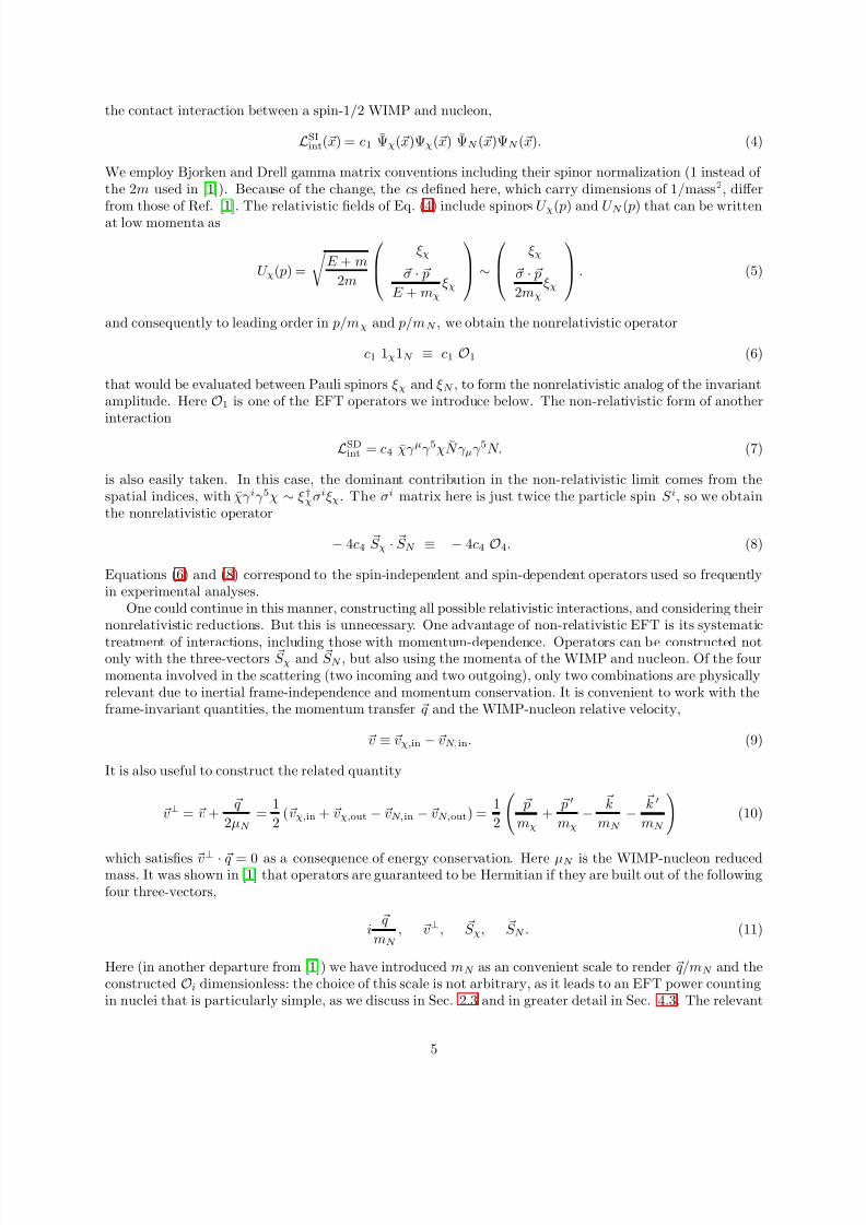
the contact interaction between a spin-1/2 WIMP and nucleon,

LSIint(x) = c1

Ψχ(x)Ψχ(x) ΨN ( x)ΨN (x). (4)

We employ Bjorken and Drell gamma matrix conventions including their spinor normalization (1 instead of the 2m used in [1]). Because of the change, the cs defined here, which carry dimensions of 1/mass2, differfrom those of Ref. [1]. The relativistic fields of Eq. (4) include spinors U

χ( p) and U

N ( p) that can be written

at low momenta as

U χ( p) =

E + m

2m

ξ χ

σ · p

E + mχξ χ

∼

ξ χ

σ · p

2mχξ χ

. (5)

and consequently to leading order in p/mχ and p/mN , we obtain the nonrelativistic operator

c1 1χ1N ≡ c1 O1 (6)

that would be evaluated between Pauli spinors ξ χ and ξ N , to form the nonrelativistic analog of the invariantamplitude. Here O1 is one of the EFT operators we introduce below. The non-relativistic form of anotherinteraction

LSDint = c4 χγ µγ 5χ N γ µγ 5N. (7)

is also easily taken. In this case, the dominant contribution in the non-relativistic limit comes from thespatial indices, with χγ iγ 5χ ∼ ξ †χσiξ χ. The σi matrix here is just twice the particle spin S i, so we obtainthe nonrelativistic operator

− 4c4 S χ · S N ≡ − 4c4 O4. (8)

Equations (6) and (8) correspond to the spin-independent and spin-dependent operators used so frequentlyin experimental analyses.

One could continue in this manner, constructing all possible relativistic interactions, and considering theirnonrelativistic reductions. But this is unnecessary. One advantage of non-relativistic EFT is its systematic

treatment of interactions, including those with momentum-dependence. Operators can be constructed notonly with the three-vectors S χ and S N , but also using the momenta of the WIMP and nucleon. Of the fourmomenta involved in the scattering (two incoming and two outgoing), only two combinations are physicallyrelevant due to inertial frame-independence and momentum conservation. It is convenient to work with theframe-invariant quantities, the momentum transfer q and the WIMP-nucleon relative velocity,

v ≡ vχ,in − vN,in. (9)

It is also useful to construct the related quantity

v⊥ = v + q

2µN =

1

2 (vχ,in + vχ,out − vN,in − vN,out) =

1

2

p

mχ+

p ′

mχ−

k

mN −

k ′

mN

(10)

which satisfies v⊥ · q = 0 as a consequence of energy conservation. Here µN is the WIMP-nucleon reducedmass. It was shown in [1] that operators are guaranteed to be Hermitian if they are built out of the followingfour three-vectors,

i q

mN , v⊥, S χ, S N . (11)

Here (in another departure from [1]) we have introduced mN as an convenient scale to render q/mN and theconstructed Oi dimensionless: the choice of this scale is not arbitrary, as it leads to an EFT power countingin nuclei that is particularly simple, as we discuss in Sec. 2.3 and in greater detail in Sec. 4.3. The relevant

5

8/17/2019 Fitzpatrick 1308.6288v1


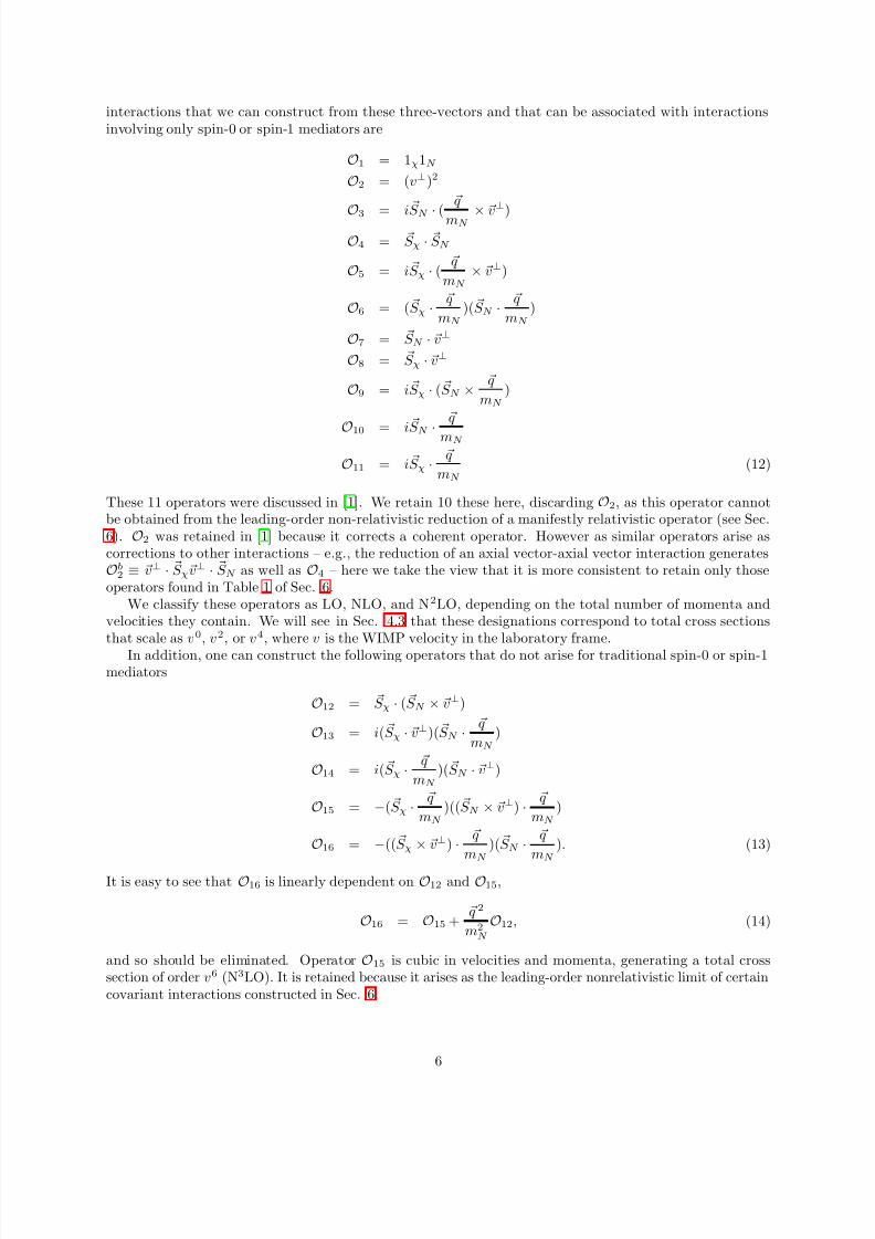
interactions that we can construct from these three-vectors and that can be associated with interactionsinvolving only spin-0 or spin-1 mediators are

O1 = 1χ1N

O2 = (v⊥)2

O3 = i S N · (

q

mN × v⊥)

O4 = S χ · S N

O5 = i S χ · ( q

mN × v⊥)

O6 = ( S χ · q

mN )( S N · q

mN )

O7 = S N · v⊥

O8 = S χ · v⊥

O9 = i S χ · ( S N × q

mN )

O10 = i S N ·

q

mN

O11 = i S χ · q

mN (12)

These 11 operators were discussed in [1]. We retain 10 these here, discarding O2, as this operator cannotbe obtained from the leading-order non-relativistic reduction of a manifestly relativistic operator (see Sec.6). O2 was retained in [1] because it corrects a coherent operator. However as similar operators arise ascorrections to other interactions – e.g., the reduction of an axial vector-axial vector interaction generatesOb

2 ≡ v⊥ · S χv⊥ · S N as well as O4 – here we take the view that it is more consistent to retain only thoseoperators found in Table 1 of Sec. 6.

We classify these operators as LO, NLO, and N2LO, depending on the total number of momenta andvelocities they contain. We will see in Sec. 4.3 that these designations correspond to total cross sectionsthat scale as v0, v2, or v4, where v is the WIMP velocity in the laboratory frame.

In addition, one can construct the following operators that do not arise for traditional spin-0 or spin-1mediators

O12 = S χ · ( S N × v⊥)

O13 = i( S χ · v⊥)( S N · q

mN )

O14 = i( S χ · q

mN )( S N · v⊥)

O15 = −( S χ · q

mN )(( S N × v⊥) · q

mN )

O16 = −(( S χ × v⊥) · q

mN )( S N · q

mN ). (13)

It is easy to see that O16 is linearly dependent on O12 and O15,

O16 = O15 + q 2

m2N

O12, (14)

and so should be eliminated. Operator O15 is cubic in velocities and momenta, generating a total crosssection of order v6 (N3LO). It is retained because it arises as the leading-order nonrelativistic limit of certaincovariant interactions constructed in Sec. 6.

6

8/17/2019 Fitzpatrick 1308.6288v1


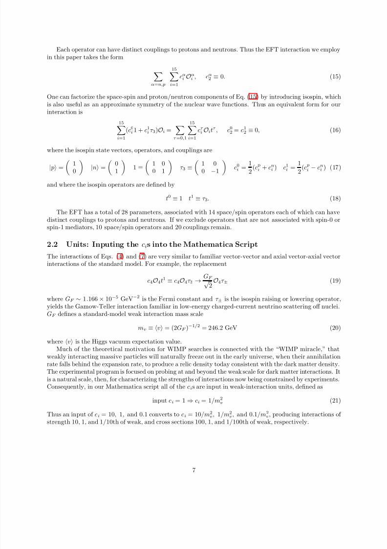
Each operator can have distinct couplings to protons and neutrons. Thus the EFT interaction we employin this paper takes the form

α=n,p

15i=1

cαi Oα

i , cα2 ≡ 0. (15)

One can factorize the space-spin and proton/neutron components of Eq. (15) by introducing isospin, whichis also useful as an approximate symmetry of the nuclear wave functions. Thus an equivalent form for ourinteraction is

15i=1

(c0i 1 + c1

i τ 3)Oi =

τ =0,1

15i=1

cτ i Oitτ , c0

2 = c12 ≡ 0, (16)

where the isospin state vectors, operators, and couplings are

| p =

10

|n =

01

1 ≡

1 00 1

τ 3 ≡

1 00 −1

c0

i = 1

2(cp

i + cni ) c1

i = 1

2(c p

i − cni ) (17)

and where the isospin operators are defined by

t0 ≡ 1 t1 ≡ τ 3. (18)

The EFT has a total of 28 parameters, associated with 14 space/spin operators each of which can havedistinct couplings to protons and neutrons. If we exclude operators that are not associated with spin-0 orspin-1 mediators, 10 space/spin operators and 20 couplings remain.

2.2 Units: Inputing the cis into the Mathematica Script

The interactions of Eqs. (4) and (7) are very similar to familiar vector-vector and axial vector-axial vectorinteractions of the standard model. For example, the replacement

c4O4t1 ≡ c4O4τ 3 → GF √ 2

O4τ ± (19)

where GF ∼ 1.166 × 10−5 GeV−2 is the Fermi constant and τ ± is the isospin raising or lowering operator,yields the Gamow-Teller interaction familiar in low-energy charged-current neutrino scattering off nuclei.GF defines a standard-model weak interaction mass scale

mv ≡ v = (2GF )−1/2 = 246.2 GeV (20)

where v is the Higgs vacuum expectation value.Much of the theoretical motivation for WIMP searches is connected with the “WIMP miracle,” that

weakly interacting massive particles will naturally freeze out in the early universe, when their annihilationrate falls behind the expansion rate, to produce a relic density today consistent with the dark matter density.The experimental program is focused on probing at and beyond the weak scale for dark matter interactions. Itis a natural scale, then, for characterizing the strengths of interactions now being constrained by experiments.

Consequently, in our Mathematica script all of the cis are input in weak-interaction units, defined as

input ci = 1 ⇒ ci = 1/m2v (21)

Thus an input of ci = 10, 1, and 0.1 converts to ci = 10/m2v, 1/m2

v, and 0.1/m2v, producing interactions of

strength 10, 1, and 1/10th of weak, and cross sections 100, 1, and 1/100th of weak, respectively.

7

8/17/2019 Fitzpatrick 1308.6288v1


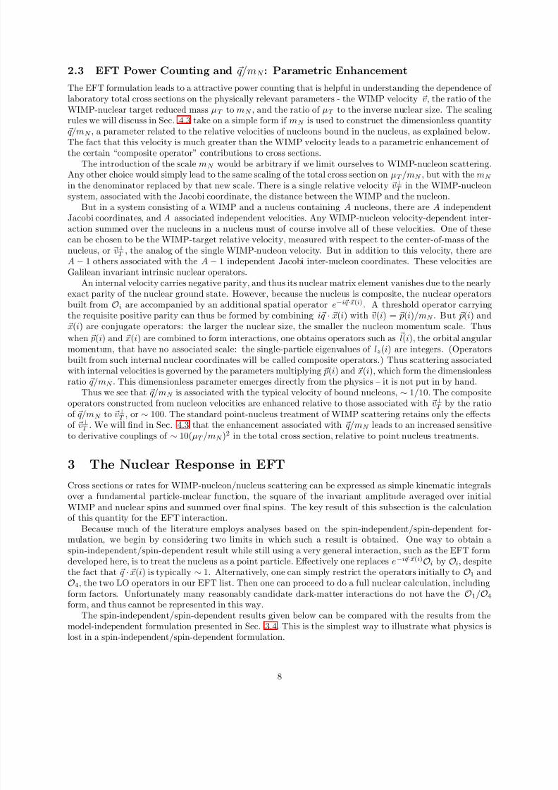
2.3 EFT Power Counting and q/mN : Parametric Enhancement

The EFT formulation leads to a attractive power counting that is helpful in understanding the dependence of laboratory total cross sections on the physically relevant parameters - the WIMP velocity v, the ratio of theWIMP-nuclear target reduced mass µT to mN , and the ratio of µT to the inverse nuclear size. The scalingrules we will discuss in Sec. 4.3 take on a simple form if mN is used to construct the dimensionless quantity q/mN , a parameter related to the relative velocities of nucleons bound in the nucleus, as explained below.The fact that this velocity is much greater than the WIMP velocity leads to a parametric enhancement of the certain “composite operator” contributions to cross sections.

The introduction of the scale mN would be arbitrary if we limit ourselves to WIMP-nucleon scattering.Any other choice would simply lead to the same scaling of the total cross section on µT /mN , but with the mN

in the denominator replaced by that new scale. There is a single relative velocity v⊥T in the WIMP-nucleonsystem, associated with the Jacobi coordinate, the distance between the WIMP and the nucleon.

But in a system consisting of a WIMP and a nucleus containing A nucleons, there are A independentJacobi coordinates, and A associated independent velocities. Any WIMP-nucleon velocity-dependent inter-action summed over the nucleons in a nucleus must of course involve all of these velocities. One of thesecan be chosen to be the WIMP-target relative velocity, measured with respect to the center-of-mass of thenucleus, or v⊥T , the analog of the single WIMP-nucleon velocity. But in addition to this velocity, there areA − 1 others associated with the A − 1 independent Jacobi inter-nucleon coordinates. These velocities are

Galilean invariant intrinsic nuclear operators.An internal velocity carries negative parity, and thus its nuclear matrix element vanishes due to the nearlyexact parity of the nuclear ground state. However, because the nucleus is composite, the nuclear operatorsbuilt from Oi are accompanied by an additional spatial operator e−i q·x(i). A threshold operator carryingthe requisite positive parity can thus be formed by combining i q · x(i) with v(i) = p(i)/mN . But p(i) andx(i) are conjugate operators: the larger the nuclear size, the smaller the nucleon momentum scale. Thus

when p(i) and x(i) are combined to form interactions, one obtains operators such as l(i), the orbital angularmomentum, that have no associated scale: the single-particle eigenvalues of lz(i) are integers. (Operatorsbuilt from such internal nuclear coordinates will be called composite operators.) Thus scattering associatedwith internal velocities is governed by the parameters multiplying p(i) and x(i), which form the dimensionlessratio q/mN . This dimensionless parameter emerges directly from the physics – it is not put in by hand.

Thus we see that q/mN is associated with the typical velocity of bound nucleons, ∼ 1/10. The compositeoperators constructed from nucleon velocities are enhanced relative to those associated with v⊥T by the ratio

of q/mN to v⊥T , or ∼ 100. The standard point-nucleus treatment of WIMP scattering retains only the effectsof v⊥T . We will find in Sec. 4.3 that the enhancement associated with q/mN leads to an increased sensitiveto derivative couplings of ∼ 10(µT /mN )

2 in the total cross section, relative to point nucleus treatments.

3 The Nuclear Response in EFT

Cross sections or rates for WIMP-nucleon/nucleus scattering can be expressed as simple kinematic integralsover a fundamental particle-nuclear function, the square of the invariant amplitude averaged over initialWIMP and nuclear spins and summed over final spins. The key result of this subsection is the calculationof this quantity for the EFT interaction.

Because much of the literature employs analyses based on the spin-independent/spin-dependent for-mulation, we begin by considering two limits in which such a result is obtained. One way to obtain a

spin-independent/spin-dependent result while still using a very general interaction, such as the EFT formdeveloped here, is to treat the nucleus as a point particle. Effectively one replaces e−i q· x(i)Oi by Oi, despitethe fact that q · x(i) is typically ∼ 1. Alternatively, one can simply restrict the operators initially to O1 andO4, the two LO operators in our EFT list. Then one can proceed to do a full nuclear calculation, includingform factors. Unfortunately many reasonably candidate dark-matter interactions do not have the O1/O4

form, and thus cannot be represented in this way.The spin-independent/spin-dependent results given below can be compared with the results from the

model-independent formulation presented in Sec. 3.4. This is the simplest way to illustrate what physics islost in a spin-independent/spin-dependent formulation.

8

8/17/2019 Fitzpatrick 1308.6288v1


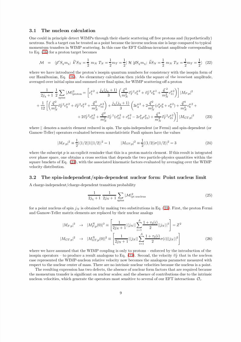
3.1 The nucleon calculation

One could in principle detect WIMPs through their elastic scattering off free protons and (hypothetically)neutrons. Such a target can be treated as a point because the inverse nucleon size is large compared to typicalmomentum transfers in WIMP scattering. In this case the EFT Galilean-invariant amplitude correspondingto Eq. (16) for a proton target becomes

M = p ′S χmχ; k′S N = 12

mN T N = 12

mT = 12| H | pS χmχ; kS N = 1

2 mN T N = 1

2mT = 1

2 (22)

where we have introduced the proton’s isospin quantum numbers for consistency with the isospin form of our Hamiltonian, Eq. (16). An elementary calculation then yields the square of the invariant amplitude,averaged over initial spins and summed over final spins, for WIMP scattering off a proton

1

2 jχ + 1

1

2

spins

|M|2proton =

c p 2

1 + jχ( jχ + 1)

3

q 2

m2N

v⊥2T c p 2

5 + v⊥2T c p 2

8 + q 2

m2N

c p 211

|M F ; p|2

+ 1

12

q 2

m2N

v⊥2T c p 2

3 + v⊥2T c p 2

7 + q 2

m2N

c p 210

+

jχ( jχ + 1)

3

3c p 2

4 + 2 q 2

m2N

(c p4c p

6 + c p 29 ) +

q 4

m4N

c p 26 +

+ 2v⊥2T c p 2

12 + q 2

m2N

v⊥ 2T (c p 2

13 + c p 214

−2c p

12c p15) +

q 4

m4N

v⊥2T c p 2

15 |M GT ; p

|2 (23)

where || denotes a matrix element reduced in spin. The spin-independent (or Fermi) and spin-dependent (orGamow-Teller) operators evaluated between nonrelativistic Pauli spinors have the values

|M F ; p|2 ≡ 1

2|1/2||1||1/2|2 = 1 |M GT ; p|2 ≡ 1

2|1/2||σ||1/2|2 = 3 (24)

where the subscript p is an explicit reminder that this is a proton matrix element. If this result is integratedover phase space, one obtains a cross section that depends the two particle-physics quantities within thesquare brackets of Eq. (23), with the associated kinematic factors evaluated by averaging over the WIMPvelocity distribution.

3.2 The spin-independent/spin-dependent nuclear form: Point nucleus limitA charge-independent/charge-dependent transition probability

1

2 jχ + 1

1

2 jN + 1

spins

|M|2pt nucleus (25)

for a point nucleus of spin jN is obtained by making two substitutions in Eq. (23). First, the proton Fermiand Gamow-Teller matrix elements are replaced by their nuclear analogs

|M F ; p|2 → |M N F ; p(0)|2 ≡

1

2 jN + 1| jN ||

Ai=1

1 + τ 3(i)

2 || jN |2

= Z 2

|M GT ; p|2

→ |M N

GT ; p(0)|2

≡ 1

2 jN + 1 | jN ||A

i=1

1 + τ 3(i)

2 σ(i)|| jN |2

(26)

where we have assumed that the WIMP coupling is only to protons – enforced by the introduction of theisospin operators – to produce a result analogous to Eq. (23). Second, the velocity v⊥T that in the nucleoncase represented the WIMP-nucleon relative velocity now becomes the analogous parameter measured withrespect to the nuclear center of mass. There are no intrinsic nuclear velocities because the nucleus is a point.

The resulting expression has two defects, the absence of nuclear form factors that are required becausethe momentum transfer is significant on nuclear scales; and the absence of contributions due to the intrinsicnucleon velocities, which generate the operators most sensitive to several of our EFT interactions Oi.

9

8/17/2019 Fitzpatrick 1308.6288v1


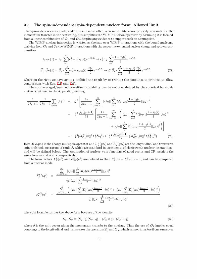
3.3 The spin-independent/spin-dependent nuclear form: Allowed limit

The spin-independent/spin-dependent result most often seen in the literature properly accounts for themomentum transfer in the scattering, but simplifies the WIMP-nucleon operator by assuming it is formedfrom a linear combination of O1 and O4, despite any evidence to support such an assumption.

The WIMP-nucleus interaction is written as the sum over WIMP interactions with the bound nucleons,deriving from

O1 and

O2 the WIMP interactions with the respective extended nuclear charge and spin-current

densities

1χρN (x) = 1χ

Ai=1

(c01 + c1

1τ 3(i))e−i q·xi → c p1 1χ

Ai=1

1 + τ 3(i)

2 e−i q·xi

S χ · jN (x) = S χ ·A

i=1

(c04 + c1

4τ 3(i))σ(i)

2 e−i q·xi → c p

4 S χ ·

Ai=1

1 + τ 3(i)

2

σ(i)

2 e−i q· xi (27)

where on the right we have again simplified the result by restricting the couplings to protons, to allowcomparisons with Eqs. (23) and (26).

The spin averaged/summed transition probability can be easily evaluated by the spherical harmonicmethods outlined in the Appendix, yielding

1

2 jχ + 1

1

2 jN + 1

spins

|M|2 = c p 21

4π

2 jN + 1

∞J =0,2,...

| jN ||A

i=1

M J (qxi)1 + τ 3(i)

2 || jN |2

+ c p 24

jχ( jχ + 1)

12

4π

2 jN + 1

∞J =1,3,...

| jN ||

Ai=1

Σ′′J (qxi)

1 + τ 3(i)

2 || jN |2

+ | jN ||A

i=1

Σ′J (qxi)

1 + τ 3(i)

2 || jN |2

≡ c p 21 |M N

F ; p(0)|2F p 2F (q 2) + c p 2

4

jχ( jχ + 1)

12 |M N

GT ; p(0)|2F p 2GT (q 2) (28)

Here M J (qxi) is the charge multipole operator and Σ′′J (qxi) and Σ′

J (qxi) are the longitudinal and transverse

spin multipole operators of rank J , which are standard in treatments of electroweak nuclear interactions,and will be defined below. The assumption of nuclear wave functions of good parity and CP restricts thesums to even and odd J , respectively.

The form factors F pF (q 2) and F pGT (q 2) are defined so that F pF (0) = F pGT (0) = 1, and can be computedfrom a nuclear model

F p 2F (q 2) =

∞J =0,2,...

| jN ||A

i=1

M J (qxi) 1+τ 3(i)2 || jN |2

14π | jN ||

Ai=1

1+τ 3(i)2 || jN |2

F

p 2

GT (q 2

) =

∞

J =1,3,...

| jN ||

A

i=1Σ′′

J (qxi)1+τ 3(i)

2 || jN |2 + | jN ||A

i=1Σ′

J (qxi)1+τ 3(i)

2 || jN |2

14π | jN ||

Ai=1

1+τ 3(i)2 σ(i)|| jN |2 .

(29)

The spin form factor has the above form because of the identity

S χ · S N ≡ ( S χ · q )( S N · q ) + ( S χ × q ) · ( S N × q ) (30)

where q is the unit vector along the momentum transfer to the nucleus. Thus the use of O4 implies equalcouplings to the longitudinal and transverse spin operators Σ′′

J and Σ′J , which cannot interfere if one sums over

10

8/17/2019 Fitzpatrick 1308.6288v1


spins. In a more general treatment of the WIMP-nucleon interaction, these operators would be independent.For example, in the EFT expansion O4 = S χ · S N and O6 = ( S χ · q )( S N · q ) have distinct coefficients.

Often in the literature F pF (q 2) and F pGT (q 2) are not calculated microscopically, but are represented bysimple phenomenological forms.

The operators M J , Σ′′J , and Σ′

J are the vector charge, axial longitudinal, and axial transverse electricmultipole operators familiar from electroweak nuclear physics. The latter two operators are also frequently

designated as L5J and T

el 5J in the literature, to emphasize their multipole and axial character.

While we have simplified the above expressions by assuming all couplings are to protons, to allow acomparison with our free-proton result, the expressions for arbitrary isospin are also simple

1

2 jχ + 1

1

2 j + 1

spins

|M|2 = 4π

2 jN + 1

∞

J =0,2,...

| jN ||A

i=1

M J (qxi)

c01 + c1

1τ 3(i) || jN ; |2

+ jχ( jχ + 1)

12

∞J =1,3,...

| jN ||

Ai=1

Σ′′J (qxi)

c0

4 + c14τ 3(i)

|| jN |2

+ | jN ||A

i=1

Σ′′J (qxi)

c0

4 + c14τ 3(i)

|| jN |2

(31)

3.4 The general EFT form of the WIMP-nucleus response

The general form of the WIMP-nucleus interaction consistent with the assumption of nuclear ground stateswith good P and CP can be derived by building an EFT at the nuclear level, or by embedding the EFTWIMP-nucleon interaction into the nucleus, without making assumptions of the sort just discussed. Wefollow the second strategy here, as it allows us to connect the nuclear responses back to the single-nucleoninteraction and consequently to the ultraviolet theories which map onto that single-nucleon interaction, onnonrelativistic reduction.

While the calculation is not difficult, we relegate most of the details to the Appendix, giving just theessentials here. First, the basic model assumption is that the nuclear interaction is the sum of the interactionsof the WIMP with the individual nucleons in the nucleus. Thus the mapping from the nucleon-level effectiveoperators to nuclear operators is made by the following generalization of Eq. (16),

τ =0,1

15i=1

cτ i Oitτ →

τ =0,1

15i=1

cτ i

Aj=1

Oi( j)tτ ( j), c02 = c1

2 = 0. (32)

Now the nuclear operators appearing in this expression are built from i q/mN , a c-number, S N , which acts onintrinsic nuclear coordinates, and the relative velocity operator v⊥, which now represents a set of A internalWIMP-nucleus system velocities, A − 1 of which involve the relative coordinates of bound nucleons (theJacobi velocities), and one of which is the velocity of the DM particle relative to the nuclear center of mass,

v⊥ →

1

2 (vχ,in + vχ,out − vN,in(i) − vN,out(i)) , i = 1,....,A

≡ v⊥

T − vN,in(i) + vN,out(i), i = 1,...,A−

1 . (33)

The DM particle/nuclear center of mass relative velocity is a c-number,

v⊥T = 1

2 (vχ,in + vχ,out − vT,in(i) − vT,out(i)) (34)

while the internal nuclear Jacobi velocities vN are operators acting on intrinsic nuclear coordinates. (That is,for a single-nucleon (A=1) target, v⊥T ≡ v⊥, while for all nuclear targets, there are A − 1 additional velocitydegrees of freedom associated with the Jacobi internucleon velocities.) This separation is discussed in moredetail in the Appendix.

11

8/17/2019 Fitzpatrick 1308.6288v1


In analogy with Eq. (27) one then obtains the WIMP-nucleus interaction

τ =0,1

lτ

0

Ai=1

e−i q·xi + lAτ 0

Ai=1

1

2M

−1

i

←−∇ i · σ(i)e−i q·xi + e−i q·xiσ(i) · 1

i

−→∇ i

+ lτ

5 ·

A

i=1

σ(i)e−i q·xi + lτ

M ·

A

i=1

1

2M −

1

i

←−∇

ie−i q·xi + e−i q·xi 1

i

−→∇

i+ lτ

E ·A

i=1

1

2M

←−∇i × σ(i)e−i q· xi + e−i q·xiσ(i) × −→∇i

int

tτ (i) (35)

where the subscript int instructs one to take the intrinsic part of the nuclear operators (that is, the partdependent on the internal Jacobi velocities). Comparing to Eq. (27), one sees that three new velocity-dependent densities appear – the nuclear axial charge operator, familiar as the β decay operator that mediates0+ ↔ 0− decays; the convection current, familiar from electromagnetism; and a spin-velocity current thatis less commonly discussed, but does arise as a higher-order correction in weak interactions. The associatedWIMP tensors contain the EFT input

lτ

0

= cτ

1

+ i( q

mN ×v⊥

T

)· S χ cτ

5

+ v⊥T ·

S χ cτ

8

+ i q

mN · S χ cτ

11

lAτ 0 = −1

2

cτ

7 + i q

mN · S χ cτ

14

l5 = 1

2

i

q

mN × v⊥T cτ

3 + S χ cτ 4 +

q

mN

q

mN · S χ cτ

6 + v⊥T cτ 7 + i

q

mN × S χ cτ

9 + i q

mN cτ

10

+v⊥T × S χ cτ 12 + i

q

mN v⊥T · S χ cτ

13 + iv⊥T

q

mN · S χ cτ

14 + q

mN × v⊥T

q

mN · S χ cτ

15

lM = i q

mN × S χ cτ

5 − S χ cτ 8

lE = 1

2

q

mN cτ

3 + i S χ cτ 12 − q

mN × S χ cτ

13 − i q

mN

q

mN · S χ cτ

15

(36)

In the Appendix the products of plane waves and scalar/vector operators appearing in Eq. (35) areexpanded in spherical and vector spherical harmonics, and the resulting amplitude is squared, averaged overinitial spins and summed over final spins. One obtains

1

2 jχ + 1

1

2 jN + 1

spins

|M|2nucleus/EFT =

4π

2 jN + 1

τ =0,1

τ ′=0,1

∞

J =0,2,...

Rτ τ ′

M (v⊥2T ,

q 2

m2N

) jN || M J ;τ (q ) || jN jN || M J ;τ ′(q ) || jN

+ q 2

m2N

Rτ τ ′

Φ′′ (v⊥2T ,

q 2

m2N

) jN || Φ′′J ;τ (q ) || jN jN || Φ′′

J ;τ ′(q ) || jN

+ q 2

m2N

Rτ τ ′

Φ′′M (v⊥2T , q 2

m2N

) jN || Φ′′J ;τ (q ) || jN jN || M J ;τ ′(q ) || jN +

∞J =2,4,...

q 2

m2N

Rτ τ ′

Φ′ (v⊥2

T , q 2

m2N

) jN || Φ′J ;τ (q ) || jN jN || Φ′

J ;τ ′(q ) || jN

+∞

J =1,3,...

Rτ τ ′

Σ′′ (v⊥2T ,

q 2

m2N

) jN || Σ′′J ;τ (q ) || jN jN || Σ′′

J ;τ ′(q ) || jN

+ Rτ τ ′

Σ′ (v⊥2T ,

q 2

m2N

) jN || Σ′J ;τ (q ) || jN jN || Σ′

J ;τ ′(q ) || jN

12

8/17/2019 Fitzpatrick 1308.6288v1


+ q 2

m2N

Rτ τ ′

∆ (v⊥2T ,

q 2

m2N

) jN || ∆J ;τ (q ) || jN jN || ∆J ;τ ′(q ) || jN

+ q 2

m2N

Rτ τ ′

∆Σ′(v⊥2T ,

q 2

m2N

) jN || ∆J ;τ (q ) || jN jN || Σ′J ;τ ′(q ) || jN

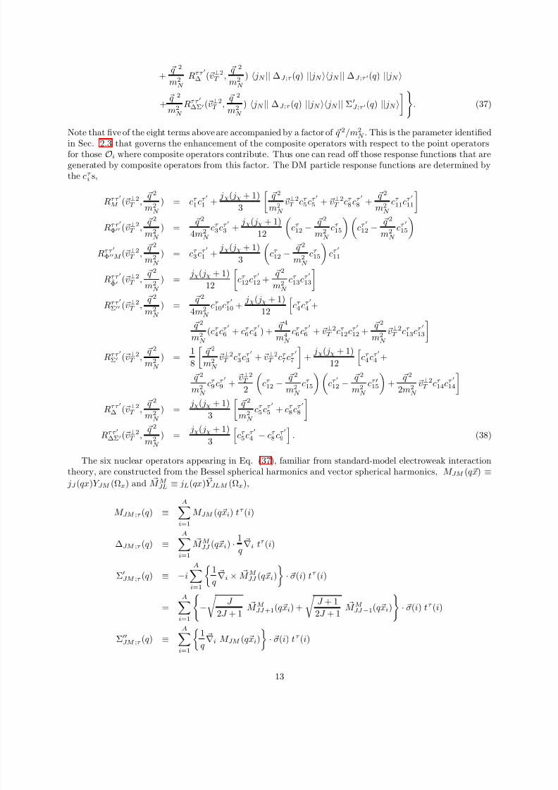
. (37)

Note that five of the eight terms above are accompanied by a factor of q 2/m2

N . This is the parameter identified

in Sec. 2.3 that governs the enhancement of the composite operators with respect to the point operatorsfor those Oi where composite operators contribute. Thus one can read off those response functions that aregenerated by composite operators from this factor. The DM particle response functions are determined bythe cτ

i s,

Rτ τ ′

M (v⊥2T ,

q 2

m2N

) = cτ 1 cτ ′

1 + jχ( jχ + 1)

3

q 2

m2N

v⊥2T cτ

5 cτ ′

5 + v⊥2T cτ

8 cτ ′

8 + q 2

m2N

cτ 11cτ ′

11

Rτ τ ′

Φ′′ (v⊥2T ,

q 2

m2N

) = q 2

4m2N

cτ 3 cτ ′

3 + jχ( jχ + 1)

12

cτ

12 − q 2

m2N

cτ 15

cτ ′

12 − q 2

m2N

cτ ′

15

Rτ τ ′

Φ′′M (v⊥2T ,

q 2

m2N

) = cτ 3 cτ ′

1 + jχ( jχ + 1)

3

cτ

12 − q 2

m2N

cτ 15

cτ ′

11

Rτ τ ′

Φ′ (v⊥2T , q 2

m2N

) = jχ( jχ + 1)12

cτ 12cτ

′

12 + q 2

m2N

cτ 13cτ ′

13

Rτ τ ′

Σ′′ (v⊥2T ,

q 2

m2N

) = q 2

4m2N

cτ 10cτ ′

10 + jχ( jχ + 1)

12

cτ

4 cτ ′

4 +

q 2

m2N

(cτ 4 cτ ′

6 + cτ 6 cτ ′

4 ) + q 4

m4N

cτ 6 cτ ′

6 + v⊥2T cτ

12cτ ′

12 + q 2

m2N

v⊥2T cτ

13cτ ′

13

Rτ τ ′

Σ′ (v⊥2T ,

q 2

m2N

) = 1

8

q 2

m2N

v⊥2T cτ

3 cτ ′

3 + v⊥2T cτ

7 cτ ′

7

+

jχ( jχ + 1)

12

cτ

4 cτ ′

4 +

q 2

m2N

cτ 9 cτ ′

9 + v⊥2

T

2

cτ

12 − q 2

m2N

cτ 15

cτ ′

12 − q 2

m2N

cτ ′15

+

q 2

2m2N

v⊥2T cτ

14cτ ′

14

Rτ τ ′

∆ (v⊥2

T ,

q 2

m2N

) = jχ( jχ + 1)

3 q 2

m2N

cτ

5

cτ ′

5 + cτ

8

cτ ′

8

Rτ τ ′

∆Σ′(v⊥2T ,

q 2

m2N

) = jχ( jχ + 1)

3

cτ

5 cτ ′

4 − cτ 8 cτ ′

9

. (38)

The six nuclear operators appearing in Eq. (37), familiar from standard-model electroweak interactiontheory, are constructed from the Bessel spherical harmonics and vector spherical harmonics, M JM (qx) ≡

jJ (qx)Y JM (Ωx) and M M JL ≡ jL(qx) Y JLM (Ωx),

M JM ;τ (q ) ≡A

i=1

M JM (qxi) tτ (i)

∆JM ;τ (q )

≡

A

i=1

M M JJ (q xi)

·

1

q

∇i tτ (i)

Σ′JM ;τ (q ) ≡ −i

Ai=1

1

q ∇i × M M

JJ (qxi)

· σ(i) tτ (i)

=A

i=1

−

J

2J + 1 M M

JJ +1(qxi) +

J + 1

2J + 1 M M

JJ −1(qxi)

· σ(i) tτ (i)

Σ′′JM ;τ (q ) ≡

Ai=1

1

q ∇i M JM (q xi)

· σ(i) tτ (i)

13

8/17/2019 Fitzpatrick 1308.6288v1


=A

i=1

J + 1

2J + 1 M M

JJ +1(qxi) +

J

2J + 1 M M

JJ −1(qxi)

· σ(i) tτ (i)

Φ′JM ;τ (q ) ≡

Ai=1

1

q ∇i × M M

JJ (qxi)

·

σ(i) × 1

q ∇i

+

1

2 M M

JJ (qxi) · σ(i)

tτ (i)

Φ′′JM ;τ (q ) ≡ i

Ai=1

1q

∇iM JM (qxi) ·σ(i) × 1

q ∇i

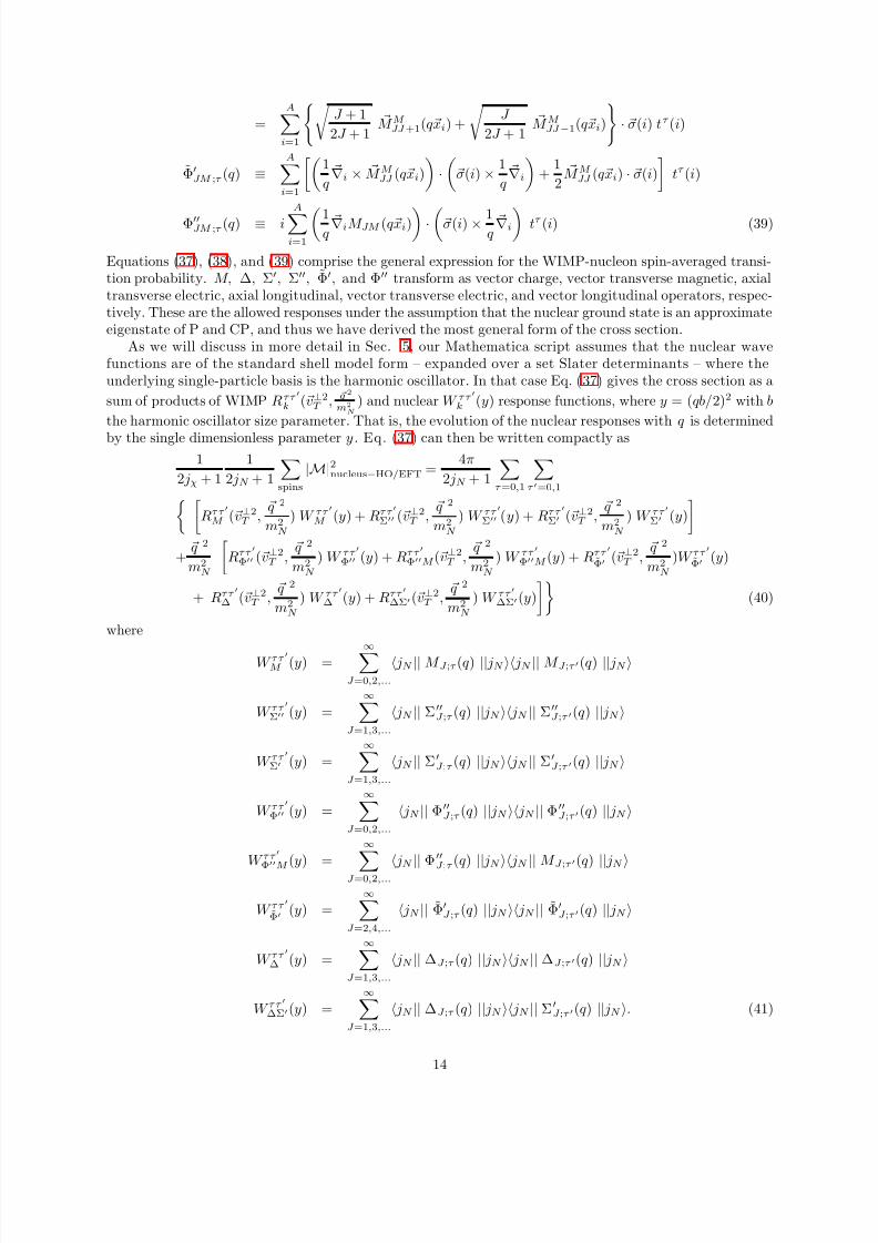
tτ (i) (39)

Equations (37), (38), and (39) comprise the general expression for the WIMP-nucleon spin-averaged transi-tion probability. M, ∆, Σ′, Σ′′, Φ′, and Φ′′ transform as vector charge, vector transverse magnetic, axialtransverse electric, axial longitudinal, vector transverse electric, and vector longitudinal operators, respec-tively. These are the allowed responses under the assumption that the nuclear ground state is an approximateeigenstate of P and CP, and thus we have derived the most general form of the cross section.

As we will discuss in more detail in Sec. 5, our Mathematica script assumes that the nuclear wavefunctions are of the standard shell model form – expanded over a set Slater determinants – where theunderlying single-particle basis is the harmonic oscillator. In that case Eq. (37) gives the cross section as a

sum of products of WIMP Rτ τ ′

k (v⊥2T , q 2

m2

N

) and nuclear W τ τ ′

k (y) response functions, where y = (qb/2)2 with b

the harmonic oscillator size parameter. That is, the evolution of the nuclear responses with q is determined

by the single dimensionless parameter y . Eq. (37) can then be written compactly as1

2 jχ + 1

1

2 jN + 1

spins

|M|2nucleus−HO/EFT =

4π

2 jN + 1

τ =0,1

τ ′=0,1

Rτ τ ′

M (v⊥2T ,

q 2

m2N

) W τ τ ′

M (y) + Rτ τ ′

Σ′′ (v⊥2T ,

q 2

m2N

) W τ τ ′

Σ′′ (y) + Rτ τ ′

Σ′ (v⊥2T ,

q 2

m2N

) W τ τ ′

Σ′ (y)

+ q 2

m2N

Rτ τ ′

Φ′′ (v⊥2T ,

q 2

m2N

) W τ τ ′

Φ′′ (y) + Rτ τ ′

Φ′′M (v⊥2T ,

q 2

m2N

) W τ τ ′

Φ′′M (y) + Rτ τ ′

Φ′ (v⊥2

T , q 2

m2N

)W τ τ ′

Φ′ (y)

+ Rτ τ ′

∆ (v⊥2T ,

q 2

m2N

) W τ τ ′

∆ (y) + Rτ τ ′

∆Σ′(v⊥2T ,

q 2

m2N

) W τ τ ′

∆Σ′(y)

(40)

where

W τ τ ′

M (y) = ∞J =0,2,...

jN || M J ;τ (q ) || jN jN || M J ;τ ′(q ) || jN

W τ τ ′

Σ′′ (y) =

∞J =1,3,...

jN || Σ′′J ;τ (q ) || jN jN || Σ′′

J ;τ ′(q ) || jN

W τ τ ′

Σ′ (y) =∞

J =1,3,...

jN || Σ′J ;τ (q ) || jN jN || Σ′

J ;τ ′(q ) || jN

W τ τ ′

Φ′′ (y) =

∞J =0,2,...

jN || Φ′′J ;τ (q ) || jN jN || Φ′′

J ;τ ′(q ) || jN

W τ τ ′

Φ′′M (y) =∞

J =0,2,...

jN

|| Φ′′

J ;τ (q ) ||

jN

jN

|| M J ;τ ′(q )

|| jN

W τ τ ′

Φ′ (y) =

∞J =2,4,...

jN || Φ′J ;τ (q ) || jN jN || Φ′

J ;τ ′(q ) || jN

W τ τ ′

∆ (y) =

∞J =1,3,...

jN || ∆J ;τ (q ) || jN jN || ∆J ;τ ′(q ) || jN

W τ τ ′

∆Σ′(y) =∞

J =1,3,...

jN || ∆J ;τ (q ) || jN jN || Σ′J ;τ ′(q ) || jN . (41)

14

8/17/2019 Fitzpatrick 1308.6288v1


Equations (40), (38), and (41) are the key formulas evaluated by the Mathematica script of Sec. 7. Parity andCP restrict the sums over multipolarities J to only even or only odd terms, depending on the transformationproperties of the operators, again as described in the Appendix.

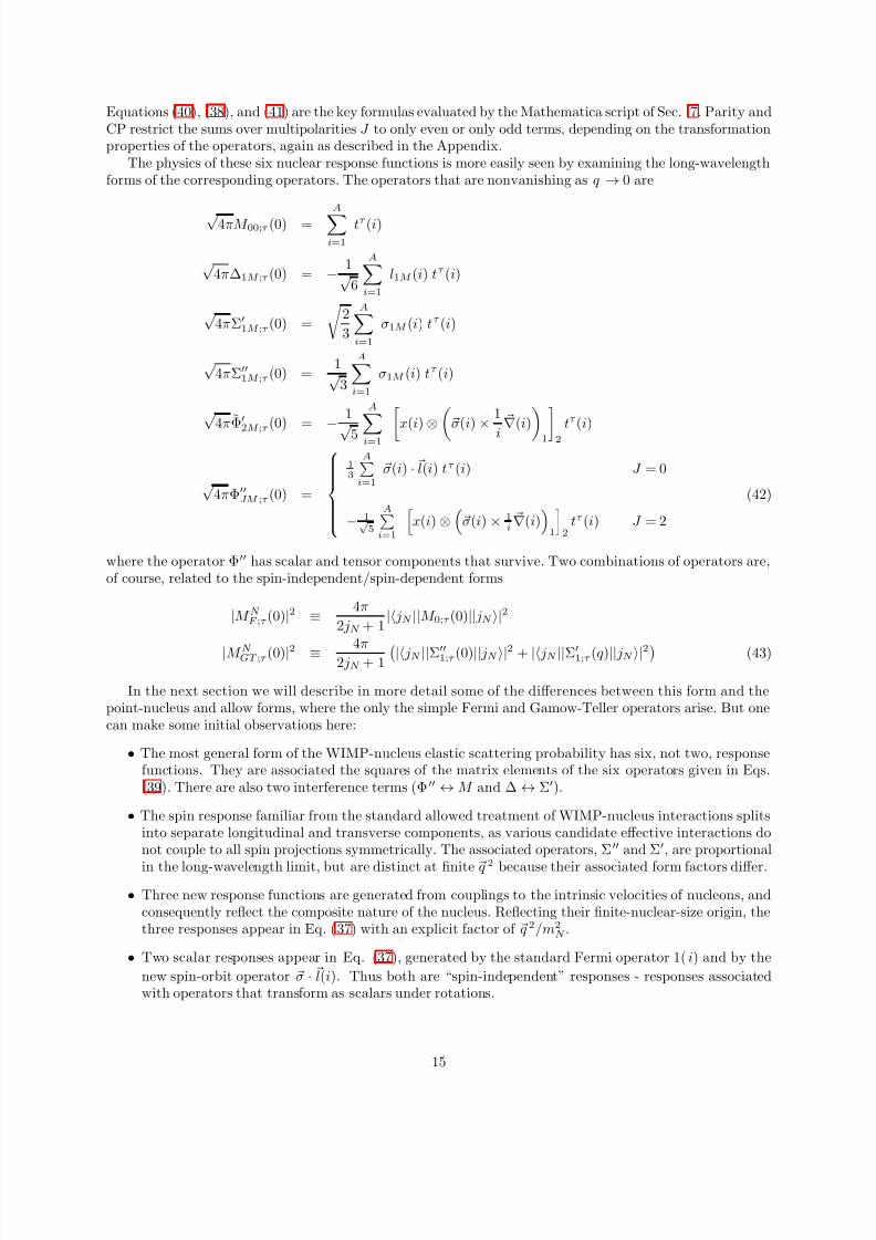
The physics of these six nuclear response functions is more easily seen by examining the long-wavelengthforms of the corresponding operators. The operators that are nonvanishing as q → 0 are

√ 4πM 00;τ (0) =A

i=1

tτ (i)

√ 4π∆1M ;τ (0) = − 1√

6

Ai=1

l1M (i) tτ (i)

√ 4πΣ′

1M ;τ (0) =

2

3

Ai=1

σ1M (i) tτ (i)

√ 4πΣ′′

1M ;τ (0) = 1√

3

Ai=1

σ1M (i) tτ (i)

√ 4πΦ′

2M ;τ (0) =

− 1

√ 5

A

i=1

x(i)

⊗σ(i)

× 1

i

∇(i)

1

2

tτ (i)

√ 4πΦ′′

JM ;τ (0) =

13

Ai=1

σ(i) · l(i) tτ (i) J = 0

− 1√ 5

Ai=1

x(i) ⊗

σ(i) × 1

i ∇(i)

1

2

tτ (i) J = 2

(42)

where the operator Φ′′ has scalar and tensor components that survive. Two combinations of operators are,of course, related to the spin-independent/spin-dependent forms

|M N F ;τ (0)|2 ≡ 4π

2 jN + 1| jN ||M 0;τ (0)|| jN |2

|M N GT ;τ (0)|2 ≡ 4π

2 jN + 1| jN ||Σ′′1;τ (0)|| jN |2 + | jN ||Σ′1;τ (q )|| jN |2

(43)

In the next section we will describe in more detail some of the differences between this form and thepoint-nucleus and allow forms, where the only the simple Fermi and Gamow-Teller operators arise. But onecan make some initial observations here:

• The most general form of the WIMP-nucleus elastic scattering probability has six, not two, responsefunctions. They are associated the squares of the matrix elements of the six operators given in Eqs.(39). There are also two interference terms (Φ′′ ↔ M and ∆ ↔ Σ′).

• The spin response familiar from the standard allowed treatment of WIMP-nucleus interactions splitsinto separate longitudinal and transverse components, as various candidate effective interactions donot couple to all spin projections symmetrically. The associated operators, Σ′′ and Σ′, are proportional

in the long-wavelength limit, but are distinct at finite q 2

because their associated form factors differ.

• Three new response functions are generated from couplings to the intrinsic velocities of nucleons, andconsequently reflect the composite nature of the nucleus. Reflecting their finite-nuclear-size origin, thethree responses appear in Eq. (37) with an explicit factor of q 2/m2

N .

• Two scalar responses appear in Eq. (37), generated by the standard Fermi operator 1(i) and by the

new spin-orbit operator σ · l(i). Thus both are “spin-independent” responses - responses associatedwith operators that transform as scalars under rotations.

15

8/17/2019 Fitzpatrick 1308.6288v1


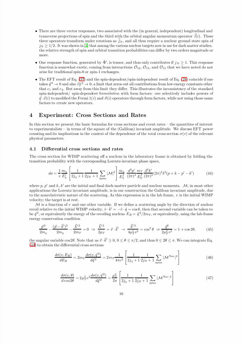
• There are three vector responses, two associated with the (in general, independent) longitudinal and

transverse projections of spin and the third with the orbital angular momentum operator l(i). Thesethree operators transform under rotations as jN , and all thus require a nuclear ground state spin of

jN ≥ 1/2. It was shown in [1] that among the various nuclear targets now in use for dark matter studies,the relative strength of spin and orbital transition probabilities can differ by two orders magnitude ormore.

• One response function, generated by Φ′, is tensor, and thus only contributes if jN ≥ 1. This responsefunction is somewhat exotic, coming from interactions O12, O13, and O15 that we have noted do notarise for traditional spin-0 or spin-1 exchanges.

• The EFT result of Eq. (37) and the spin-dependent/spin-independent result of Eq. (28) coincide if onetakes q 2 → 0 and also v⊥2

T → 0, a limit that zeros out all contributions from low-energy constants otherthat c1 and c4. But away from this limit they differ. This illustrates the inconsistency of the standardspin-independent/ spin-dependent formulation with form factors: one selectively includes powers of q · x(i) to modified the Fermi 1(i) and σ(i) operators through form factors, while not using those samefactors to create new operators.

4 Experiment: Cross Sections and Rates

In this section we present the basic formulas for cross sections and event rates – the quantities of interestto experimentalists – in terms of the square of the (Galilean) invariant amplitude. We discuss EFT powercounting and its implications in the context of the dependence of the total cross section σ(v) of the relevantphysical parameters.

4.1 Differential cross sections and rates

The cross section for WIMP scattering off a nucleus in the laboratory frame is obtained by folding thetransition probability with the corresponding Lorentz-invariant phase space,

dσ = 1

v

mχ

E iχ

1

2 jχ + 1

1

2 jN + 1 spins

|M|2

mχ

E f χ

d3 p′

(2π)3

mT

E f T

d3k′

(2π)3(2π)4δ 4( p + k − p′ − k′) (44)

where p, p′ and k , k′ are the initial and final dark-matter particle and nuclear momenta. M, in most otherapplications the Lorentz invariant amplitude, is in our construction the Galilean invariant amplitude, dueto the nonrelativistic nature of the scattering. As this expression is in the lab frame, v is the initial WIMPvelocity; the target is at rest.

M is a function of v and one other variable. If we define a scattering angle by the direction of nuclearrecoil relative to the initial WIMP velocity, v · k′ = −v · q = cos θ, then that second variable can be taken tobe q 2, or equivalently the energy of the recoiling nucleus E R = q 2/2mT , or equivalently, using the lab-frameenergy conservation condition

p 2

2mχ− ( p − k′)2

2mχ−

k′ 2

2mT = 0 ⇒

k′ 2

2µT = v · k′ →

k′ 2

4µ2T v

2 = cos2 θ ⇒ q 2

2µ2T v

2 = 1 + cos 2θ, (45)

the angular variable cos2θ. Note that as v · k′ ≥ 0, 0 ≤ θ ≤ π/2, and thus 0 ≤ 2θ ≤ π. We can integrate Eq.(44) to obtain the differential cross sections

dσ(v, E R)

dE R= 2mT

dσ(v, q 2)

d q 2 = 2mT

1

4πv2

1

2 jχ + 1

1

2 jN + 1

spins

|MNuc |2

(46)

dσ(v, θ)

d cos2θ = 2µ2

T v2 dσ(v, q 2)

d q 2 =

µ2T

2π

1

2 jχ + 1

1

2 jN + 1

spins

|MNuc |2

(47)

16

8/17/2019 Fitzpatrick 1308.6288v1


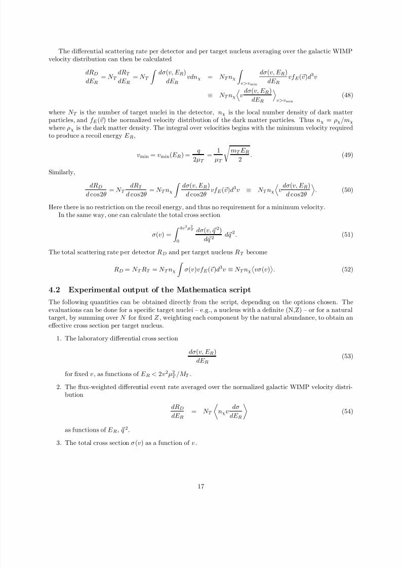
The differential scattering rate per detector and per target nucleus averaging over the galactic WIMPvelocity distribution can then be calculated

dRD

dE R= N T

dRT

dE R= N T

dσ(v, E R)

dE Rvdnχ = N T nχ

v>vmin

dσ(v, E R)

dE Rvf E (v)d3v

≡ N T nχv

dσ(v, E R)

dE R

v>vmin

(48)

where N T is the number of target nuclei in the detector, nχ is the local number density of dark matterparticles, and f E (v) the normalized velocity distribution of the dark matter particles. Thus nχ = ρχ/mχ

where ρχ is the dark matter density. The integral over velocities begins with the minimum velocity requiredto produce a recoil energy E R,

vmin = vmin(E R) = q

2µT =

1

µT

mT E R

2 . (49)

Similarly,

dRD

d cos2θ = N T

dRT

d cos2θ = N T nχ

dσ(v, E R)

d cos2θ vf E (v)d3v ≡ N T nχv

dσ(v, E R)

d cos2θ . (50)

Here there is no restriction on the recoil energy, and thus no requirement for a minimum velocity.In the same way, one can calculate the total cross section

σ(v) =

4v2µ2

T

0

dσ(v, q 2)

d q 2 d q 2. (51)

The total scattering rate per detector RD and per target nucleus RT become

RD = N T RT = N T nχ

σ(v)vf E (v)d3v ≡ N T nχ

vσ(v)

. (52)

4.2 Experimental output of the Mathematica script

The following quantities can be obtained directly from the script, depending on the options chosen. Theevaluations can be done for a specific target nuclei – e.g., a nucleus with a definite (N,Z) – or for a naturaltarget, by summing over N for fixed Z , weighting each component by the natural abundance, to obtain aneffective cross section per target nucleus.

1. The laboratory differential cross section

dσ(v, E R)

dE R(53)

for fixed v , as functions of E R < 2v2µ2T /M T .

2. The flux-weighted differential event rate averaged over the normalized galactic WIMP velocity distri-

butiondRD

dE R= N T

nχv

dσ

dE R

(54)

as functions of E R, q 2.

3. The total cross section σ(v) as a function of v .

17

8/17/2019 Fitzpatrick 1308.6288v1


8/17/2019 Fitzpatrick 1308.6288v1


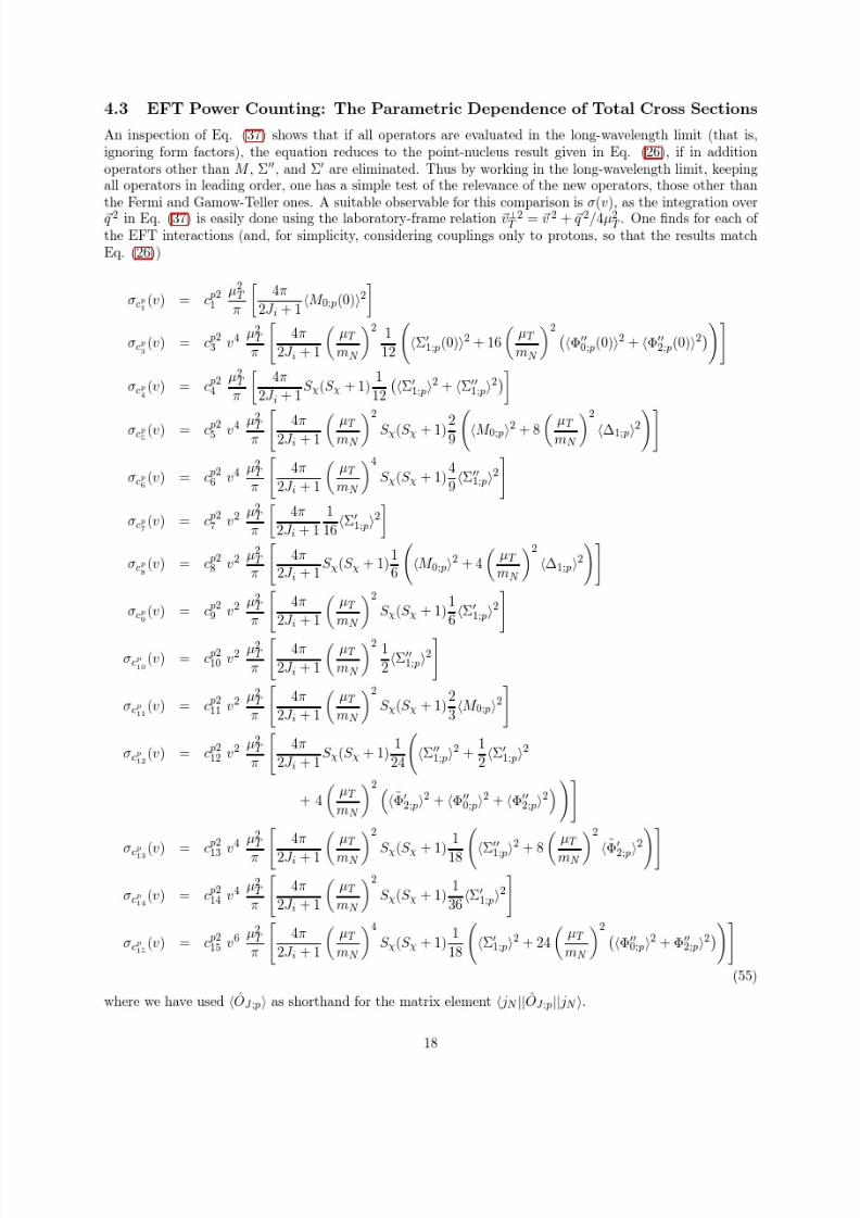
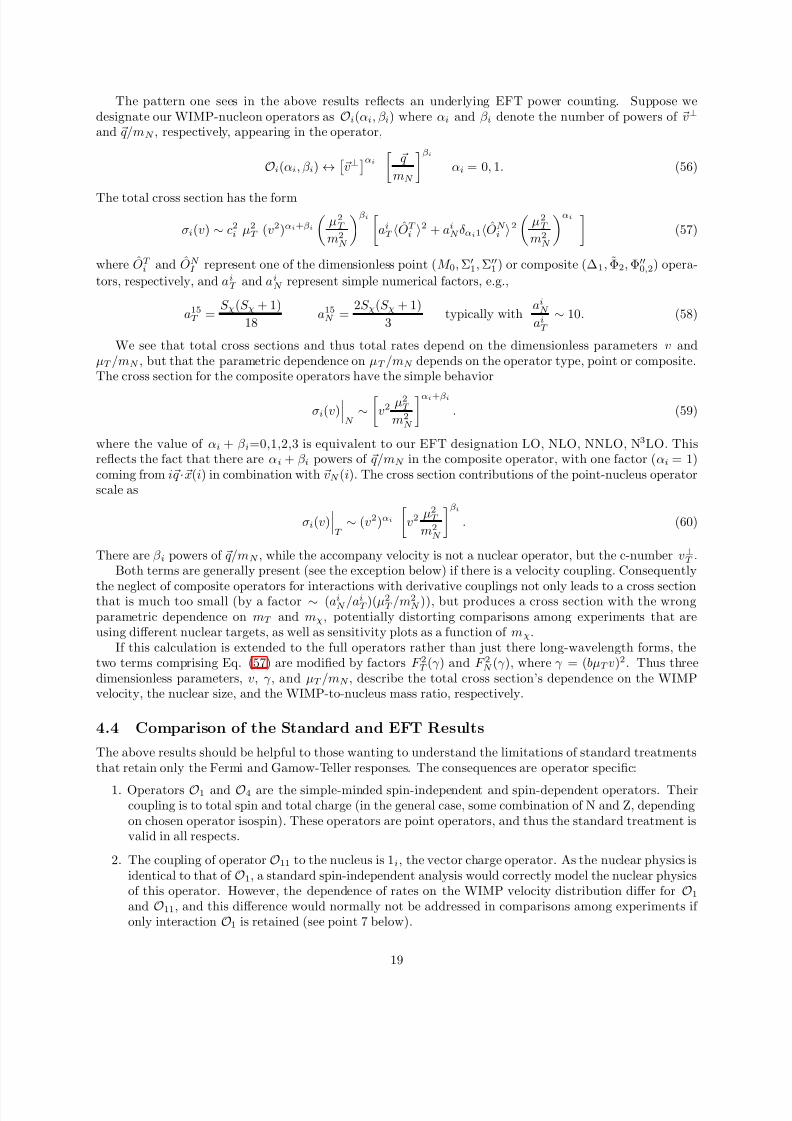
The pattern one sees in the above results reflects an underlying EFT power counting. Suppose wedesignate our WIMP-nucleon operators as Oi(αi, β i) where αi and β i denote the number of powers of v⊥

and q/mN , respectively, appearing in the operator,

Oi(αi, β i) ↔v⊥

αi

q

mN

βi

αi = 0, 1. (56)

The total cross section has the form

σi(v) ∼ c2i µ2

T (v2)αi+βi

µ2

T

m2N

βi ai

T OT i 2 + ai

N δ αi1ON i 2

µ2

T

m2N

αi

(57)

where OT i and ON

I represent one of the dimensionless point (M 0, Σ′1, Σ′′

1 ) or composite (∆1, Φ2, Φ′′0,2) opera-

tors, respectively, and aiT and ai

N represent simple numerical factors, e.g.,

a15T =

S χ(S χ + 1)

18 a15

N = 2S χ(S χ + 1)

3 typically with

aiN

aiT

∼ 10. (58)

We see that total cross sections and thus total rates depend on the dimensionless parameters v andµT /mN , but that the parametric dependence on µT /mN depends on the operator type, point or composite.The cross section for the composite operators have the simple behavior

σi(v)

N ∼

v2 µ2T

m2N

αi+βi

. (59)

where the value of αi + β i=0,1,2,3 is equivalent to our EFT designation LO, NLO, NNLO, N3LO. Thisreflects the fact that there are αi + β i powers of q/mN in the composite operator, with one factor (αi = 1)coming from i q ·x(i) in combination with vN (i). The cross section contributions of the point-nucleus operatorscale as

σi(v)

T ∼ (v2)αi

v2 µ2

T

m2N

βi

. (60)

There are β i powers of q/mN , while the accompany velocity is not a nuclear operator, but the c-number v⊥T .Both terms are generally present (see the exception below) if there is a velocity coupling. Consequently

the neglect of composite operators for interactions with derivative couplings not only leads to a cross sectionthat is much too small (by a factor ∼ (aiN /ai

T )(µ2T /m2

N )), but produces a cross section with the wrongparametric dependence on mT and mχ, potentially distorting comparisons among experiments that areusing different nuclear targets, as well as sensitivity plots as a function of mχ.

If this calculation is extended to the full operators rather than just there long-wavelength forms, thetwo terms comprising Eq. (57) are modified by factors F 2T (γ ) and F 2N (γ ), where γ = (bµT v)2. Thus threedimensionless parameters, v, γ , and µT /mN , describe the total cross section’s dependence on the WIMPvelocity, the nuclear size, and the WIMP-to-nucleus mass ratio, respectively.

4.4 Comparison of the Standard and EFT Results

The above results should be helpful to those wanting to understand the limitations of standard treatmentsthat retain only the Fermi and Gamow-Teller responses. The consequences are operator specific:

1. Operators O1 and O4 are the simple-minded spin-independent and spin-dependent operators. Theircoupling is to total spin and total charge (in the general case, some combination of N and Z, dependingon chosen operator isospin). These operators are point operators, and thus the standard treatment isvalid in all respects.

2. The coupling of operator O11 to the nucleus is 1i, the vector charge operator. As the nuclear physics isidentical to that of O1, a standard spin-independent analysis would correctly model the nuclear physicsof this operator. However, the dependence of rates on the WIMP velocity distribution differ for O1

and O11, and this difference would normally not be addressed in comparisons among experiments if only interaction O1 is retained (see point 7 below).

19

8/17/2019 Fitzpatrick 1308.6288v1


3. The operators O6 and O10 couple to the nucleus through longitudinal spin, q · σ(i), while O9 couplesthrough transverse spin, q ×σ(i). For these operators, the standard analysis based on a spin-dependentcoupling would yield the right threshold ( q → 0) coupling to the nucleus, but misrepresent the formfactors (as Σ′ and Σ′′ are described by distinct form factors). The predicted dependence of rates on thegalactic WIMP velocity distribution also differs from the standard O4 interaction (see point 7 below).

4. The operators O3

, O5

, O8

, O12

, O13

, and O15

involve velocity-dependent couplings to the nucleus.The standard spin-independent/spin-dependent analysis grossly misrepresents the physics of theseoperators, leading to errors that can exceed several orders of magnitude. They couple dominantlythrough the new composite operators ∆, Φ′, and Φ′′: the contributions of these operators to thecross section are parametrically enhanced relative to those of the standard operators by the factor(4 − 24) × (µT /mN )

2 ∼ 10A2. The resulting large errors can be partially mitigated in the case of O5

and O8 because the new operators compete with M 0, which can be coherent if isospin couplings aredialed to make the operator primarily isoscalar. But even in this favorable case, the error can be anorder of magnitude.

5. In all of the cases above, the standard treatment would distort the multipolarity of the coupling. Op-erators O3, O12, O13, and O15 would appear in the standard treatment as spin-dependent interactions,coupling through Σ′

1 and Σ′′1 , and thus could be probed only if the target has jN ≥ 1/2. In fact, O3,

O12, and

O15 have dominant scalar couplings through Φ′′

0 , which we have noted is proportional to

σ(i) · l(i) – an operator that is not only scalar, but is quasi-coherent, as discussed in [1]. The dominantcontribution from O13 is through the tensor operator Φ′

2, which requires jN ≥ 1, a possibility totallyoutside the standard description.

6. Two operators remain that at first appear puzzling: O7 and O14 have velocity-dependent couplingsto the nucleus, but unlike the operators discussing in point 5, they have standard spin-dependentcouplings, and no contribution from the new composite operators. This result is a consequence of the good P and CP of nuclear wave functions. These operators couple to the nucleus through theaxial-charge, S N · v⊥. When one combines S N · v⊥ with e−i q·xi to produce multipole operators in thestandard way, the matrix elements of the even multipoles vanish by parity, while those of the oddmultipoles vanish by CP (or, equivalently, time-reversal invariance). Consequently all contributions of intrinsic velocities to O7 and O14 vanish. Thus the only contribution to the axial charge operator thatsurvives is the single degree-of-freedom corresponding to the nuclear center-of-mass velocity. As thisvelocity is a c-number, the associated nuclear coupling is a conventional spin operator, Σ′

1.

7. By adopting an interaction having the form O1 or O4, one builds in the assumption that detector ratesdepend on the v0 moment of the galactic velocity distribution. This assumption is generally in errorfor operators other than O1 and O4, even if the operator is one of those described in points 2 and 3above, with nuclear physics quite similar to O1 and O4. The rates for LO, NLO, NNLO,..., operatorsdepend on the v0, v2, v4, ..., moments, respectively, of the WIMP velocity distribution. Consequentthe distribution of events as a function of recoil energy E R could be used to discriminate among classesof candidate interactions.

5 Nuclear Structure Input: Density Matrices

The Mathematica script described in Sec. 7 is designed to allow a nuclear structure theorist to supplyalternative descriptions of the nuclear physics, without requiring him/her to have any detailed knowledgeof the operator matrix elements that must be calculated. This is accomplished through the use of densitymatrices.

The dark matter particle scattering cross sections are expressed in terms of the single-reduced (in angularmomentum) matrix elements of one-body operators of definite angular momentum. In the treatment so farwe have labeled the nuclear ground state by its angular momentum jN , an exact quantum number. Here weadd to that label the isospin quantum numbers T , M T : isospin T is an approximate but not exact quantumlabel, as isospin is broken by the electromagnetic interactions among nucleons. However, we employ thatlabel here because most shell-model calculations are isospin conserving, and thus most density matrices

20

8/17/2019 Fitzpatrick 1308.6288v1


derived from such calculations employ T as a quantum label. We stress, however, that everything discussedbelow can be trivially repeated without the assumption of T as a nuclear state label: the density matrixwould then be defined without this assumption.

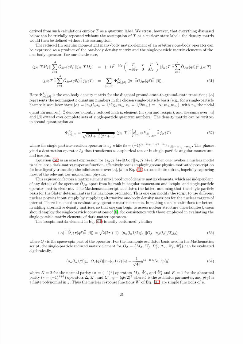
The reduced (in angular momentum) many-body matrix element of an arbitrary one-body operator canbe expressed as a product of the one-body density matrix and the single-particle matrix elements of theone-body operator. For our elastic case,

jN ; T M T ||A

i=1

OJ ;τ (qxi)|| jN ; T M T = (−1)T −M T

T τ T −M T 0 M T

jN ; T

......

Ai=1

OJ ;τ (qxi)...... jN ; T

jN ; T ......

Ai=1

OJ ;τ (qxi)...... jN ; T =

|α|,|β|

ΨJ ;τ |α|,|β| |α| ...

...OJ ;τ (qx)...... |β |. (61)

Here ΨJ ;τ |α|,|β| is the one-body density matrix for the diagonal ground-state-to-ground-state transition; |α|

represents the nonmagnetic quantum numbers in the chosen single-particle basis (e.g., for a single-particleharmonic oscillator state |α = |nα(lαsα = 1/2) jαmjα ; tα = 1/2mtα ≡ ||α|; mjαmtα, with nα the nodal

quantum number);...... denotes a doubly reduced matrix element (in spin and isospin); and the sums over |α|

and

|β

| extend over complete sets of single-particle quantum numbers. The density matrix can be written

in second quantization as

ΨJ ;τ |α|,|β| ≡

1 (2J + 1)(2τ + 1)

jN ; T ......

c†|α| ⊗ c|β|

J ;τ

...... jN ; T (62)

where the single particle creation operator is c†α while cβ = (−1)jβ−mjβ+1/2−mtβ c|β|;−mjβ

,−mtβ. The phases

yield a destruction operator cβ that transforms as a spherical tensor in single-particle angular momentumand isospin.

Equation (61) is an exact expression for jN ; T M T ||OJ ; τ || jN ; T M T . When one invokes a nuclear modelto calculate a dark-matter response function, effectively one is employing some physics-motivated prescriptionfor intelligently truncating the infinite sums over |α|, |β | in Eq. (61) to some finite subset, hopefully capturingmost of the relevant low-momentum physics.

This expression factors a matrix element into a product of density matrix elements, which are independentof any details of the operator OJ ;τ apart from its rank in angular momentum and isospin, and single-particleoperator matrix elements. The Mathematica script calculates the latter, assuming that the single-particlebasis for the Slater determinants is the harmonic oscillator. Thus one can modify the script to use differentnuclear physics input simply by supplying alternative one-body density matrices for the nuclear targets of interest. There is no need to evaluate any operator matrix elements. In making such substitutions (or better,in adding alternative density matrices, so that one can begin to assess nuclear structure uncertainties), usersshould employ the single-particle conventions of [8], for consistency with those employed in evaluating thesingle-particle matrix elements of dark-matter operators.

The isospin matrix element in Eq. (61) is easily performed, yielding

|α| ...... OJ ; τ (qx)

...... |β | =

2(2τ + 1) nα(lα1/2) jα ||OJ || nβ(lβ 1/2) jβ (63)

where OJ is the space-spin part of the operator. For the harmonic oscillator basis used in the Mathematicascript, the single-particle reduced matrix element for OJ = M J , Σ′

J , Σ′′J , ∆J , Φ′

J , Φ′′J can be evaluated

algebraically,

nα(lα1/2) jα||OJ (q x)||nβ (lβ 1/2) jβ = 1√

4πy(J −K )/2e−y p(y) (64)

where K = 2 for the normal parity (π = (−1)J ) operators M J , Φ′J , and Φ′′

J and K = 1 for the abnormalparity (π = (−1)J +1) operators ∆, Σ′, and Σ′′. y = (qb/2)2 where b is the oscillator parameter, and p(y) isa finite polynomial in y . Thus the nuclear response functions W of Eq. (41) are simple functions of y .

21

8/17/2019 Fitzpatrick 1308.6288v1


8/17/2019 Fitzpatrick 1308.6288v1


6 Particle Theory Input: Nonrelativistic Matching

In most cases a theorist interested in a given ultraviolet theory of dark matter will derive a relativistic WIMP-nucleon interaction Lint. The Mathematica script is set up to allow one to 1) input the coefficients ci of thenonrelativistic Galilean-invariant operators Oi directly (the choice one would likely make in experimentalanalysis); or alternatively 2) input the coefficients dj of a set of such covariant interactions amplitudes Lj

int,

which are then reduced to the form

i ciOi.

6.1 The L jint

In Sec. 2 we discussed two simple examples of 2), the spin-independent and spin-dependent interactionsLSI

int and LSDint . The invariant amplitudes obtained from these L were reduced to their nonrelativistic forms,

yielding matrix elements between Pauli spinors. The nonrelativistic operators between the Pauli spinorswere identified as O1 and O4. Here we repeat the process for large set of Lj

int listed in Table 1. Unlike

the simple cases discussed in Sec. 2, the Ljint do not always map onto single nonrelativistic operators Oj .

Instead the result is frequently

Ljint →

i

ci( j)Oi. (65)

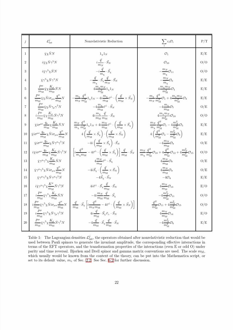
where several ci( j) are nonzero.The interactions of Table 1, coded into our Mathematic script, describe the interactions of spin-1/2

WIMPS with nucleons. (More general interactions could be considered, of course.) Four-momentum defini-tions follow our three-momentum conventions: the incoming (outgoing) four-momentum of the dark matterparticle χ is pµ ( p′µ); the incoming (outgoing) four-momentum of the nucleon N is kµ (k′µ); and the mo-mentum transfer q µ = p′µ − pµ = kµ − k′µ. We also define P µ = pµ + p′µ and K µ = kµ + k′µ. The relativevelocity operator of Eq. (10) can be written in term of these variables as

v⊥ ≡ 1

2 (vχ,in + vχ,out − vN,in − vN,out) =

1

2

P

mχ−

K

mN

. (66)

The relativistic WIMP-nucleon interactions are constructed as bilinear WIMP-nucleon products of the avail-

able scalar (χχ, χγ 5

χ) and four-vector (χP µ

χ, χP µ

γ 5

χ, χiσµν

q ν χ, and χγ µ

γ 5

χ) amplitudes. Thus thereare 22 + 42 = 20 combinations [1]. The nonrelativistic operators obtained after nonrelativistic reductionare listed in Table 1, along with the corresponding expansions in terms of our EFT operators, the Oi. TheTable also gives transformation properties of the interactions under parity and time-reversal. Note that allinteractions reduce in leading order to combinations of our fifteen Oi, and all of the Oi appear in the Table.Thus they are the minimal set of nonrelativistic interactions needed to represent the listed set of 20 Lj

int.

6.2 Units: Inputing the d js into the Mathematic Script

The Mathematica script allows one to specific an interaction corresponding to an arbitrary sum over theterms in Table 1. It then calculates the corresponding operator, expressing it in terms of the Oi, that oneuses between Paul spinors to calculate the WIMP-nucleon (Galilean) invariant amplitude. Thus

j

djLj

int → i

ciOi (67)

where the ci are functions of the dj. The Ljint of the Table all have the same dimension, as the dimensionless

quantities P µ/mM , K µ/mM and q µ/mM were used in the operator construction. Here mM is a mass scalethat will generally be known, given a model context. The dj , like the cj , have dimensions 1/mass2. Hence theconversion of a dj to a linear combination of the ci involves an expression with only dimensionless coefficients.

In analogy with input for the cj, the dj are input in units of 1/m2M . That is

input dj = 1 ⇒ dj = 1/m2M . (68)

23

8/17/2019 Fitzpatrick 1308.6288v1


The user is queried about the desired input value for mM . If no value is specified, the script defaults tothe choice mM = mv = 246.2 GeV, weak interaction strength. Note that the value of mM is used both inEq. (68), converting input numbers into appropriately dimensioned couplings dj , as well as in defining themomentum-dependent operators appearing in the Table.

7 The Mathematica Script: DocumentationThe formalism presented in this paper, with its factorization cross sections into products of WIMP andnuclear responses, is the basis for the Mathematica script presented here. The script was constructed so thatexperimental groups would be able to conduct model independent analyses of their experiments using theEFT framework. We have integrated the particle and nuclear physics in ways that should make the codeuseful to nuclear structure and particle theorists as well, as described in previous sections.

In this section, which also serves as a readme file for the program, we discuss the usage of the programitself.

7.1 Initialization

Our Mathematica package, along with all of the associated documentation, can be found athttp://www.ocf.berkeley.edu/

~nanand/software/dmformfactor/. To initialize the package, either put

dmformfactor.m in your directory for Mathematica packages and run

<<‘dmformfactor

or initialize the package file itself from its source directory. For example

<<"/Users/me/myfiles/dmformfactor.m"

7.2 Summary of Functions

In order to compute the WIMP response functions Rτ τ ′

i (v⊥2T , q 2

m2

N

), the user must first call functions setting

the dark matter mass and spin as well as the coefficients of the effective Lagrangian. In order to computethe nuclear response functions W i((qb/2)2), the user must specify the Z and A of the isotope. The densitymatrices and the oscillator parameter b needed in the calculation of the W i are set internally in the script,though there are options to override the internal values. The nuclear ground state spin and isospin (thescript assumes exact isospin, consistent with an input density matrix that is doubly reduced - see text) arealso set internally, once Z and A are input.

• SetJChi and SetMChi: These set the dark matter spin and mass, respectively. Simply call:

SetJChi[j]

and

SetMChi[m]

to set the dark matter spin to j and the dark matter mass to m. The unit GeV is recognized by thescript; for example, calling SetMChi[10 GeV] sets the dark matter mass to 10 GeV.

24

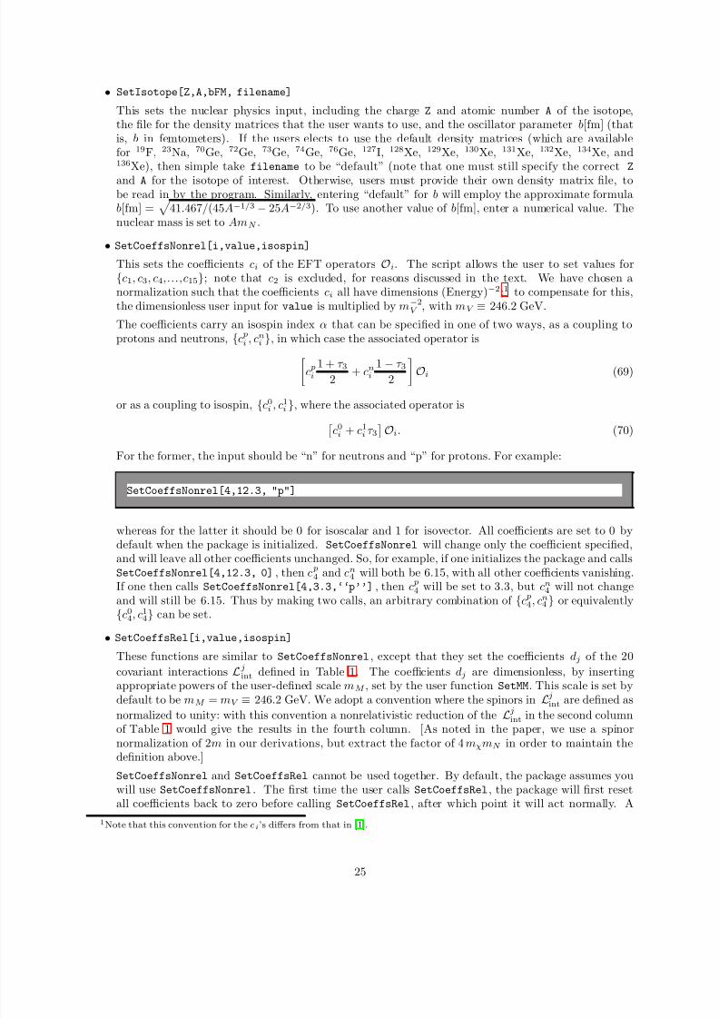
http://www.ocf.berkeley.edu/~nanand/software/dmformfactor/





8/17/2019 Fitzpatrick 1308.6288v1


• SetIsotope[Z,A,bFM, filename]

This sets the nuclear physics input, including the charge Z and atomic number A of the isotope,the file for the density matrices that the user wants to use, and the oscillator parameter b[fm] (thatis, b in femtometers). If the users elects to use the default density matrices (which are availablefor 19F, 23Na, 70Ge, 72Ge, 73Ge, 74Ge, 76Ge, 127I, 128Xe, 129Xe, 130Xe, 131Xe, 132Xe, 134Xe, and136Xe), then simple take filename to be “default” (note that one must still specify the correct Z

and A for the isotope of interest. Otherwise, users must provide their own density matrix file, tobe read in by the program. Similarly, entering “default” for b will employ the approximate formulab[fm] =

41.467/(45A−1/3 − 25A−2/3). To use another value of b[fm], enter a numerical value. The

nuclear mass is set to AmN .

• SetCoeffsNonrel[i,value,isospin]

This sets the coefficients ci of the EFT operators Oi. The script allows the user to set values forc1, c3, c4,...,c15; note that c2 is excluded, for reasons discussed in the text. We have chosen anormalization such that the coefficients ci all have dimensions (Energy)−2;1 to compensate for this,the dimensionless user input for value is multiplied by m−2

V , with mV ≡ 246.2 GeV.

The coefficients carry an isospin index α that can be specified in one of two ways, as a coupling toprotons and neutrons, c p

i , cni , in which case the associated operator is

c pi

1 + τ 32

+ cni

1 − τ 32

Oi (69)

or as a coupling to isospin, c0i , c1

i , where the associated operator isc0

i + c1i τ 3

Oi. (70)

For the former, the input should be “n” for neutrons and “p” for protons. For example:

SetCoeffsNonrel[4,12.3, "p"]

whereas for the latter it should be 0 for isoscalar and 1 for isovector. All coefficients are set to 0 bydefault when the package is initialized. SetCoeffsNonrel will change only the coefficient specified,and will leave all other coefficients unchanged. So, for example, if one initializes the package and callsSetCoeffsNonrel[4,12.3, 0], then c p

4 and cn4 will both be 6.15, with all other coefficients vanishing.

If one then calls SetCoeffsNonrel[4,3.3,‘‘p’’], then c p4 will be set to 3.3, but cn

4 will not changeand will still be 6.15. Thus by making two calls, an arbitrary combination of c p

4, cn4 or equivalently

c04, c1

4 can be set.

• SetCoeffsRel[i,value,isospin]

These functions are similar to SetCoeffsNonrel, except that they set the coefficients dj of the 20

covariant interactions Ljint defined in Table 1. The coefficients dj are dimensionless, by inserting

appropriate powers of the user-defined scale mM , set by the user function SetMM. This scale is set bydefault to be mM = mV

≡246.2 GeV. We adopt a convention where the spinors in

Ljint are defined as

normalized to unity: with this convention a nonrelativistic reduction of the Ljint in the second columnof Table 1 would give the results in the fourth column. [As noted in the paper, we use a spinornormalization of 2m in our derivations, but extract the factor of 4mχmN in order to maintain thedefinition above.]

SetCoeffsNonrel and SetCoeffsRel cannot be used together. By default, the package assumes youwill use SetCoeffsNonrel. The first time the user calls SetCoeffsRel, the package will first resetall coefficients back to zero before calling SetCoeffsRel, after which point it will act normally. A

1Note that this convention for the ci’s differs from that in [1].

25

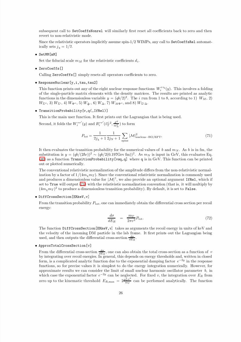
8/17/2019 Fitzpatrick 1308.6288v1


subsequent call to SetCoeffsNonrel will similarly first reset all coefficients back to zero and thenrevert to non-relativistic mode.

Since the relativistic operators implicitly assume spin-1/2 WIMPs, any call to SetCoeffsRel automat-ically sets jχ = 1/2.

• SetMM[mM]

Set the fiducial scale mM for the relativistic coefficients di.

• ZeroCoeffs[]

Calling ZeroCoeffs[] simply resets all operators coefficients to zero.

• ResponseNuclear[y,i,tau,tau2]

This function prints out any of the eight nuclear response functions W τ τ 2i (y). This involves a folding

of the single-particle matrix elements with the density matrices. The results are printed as analyticfunctions in the dimensionless variable y = (qb/2)2. The i run from 1 to 8, according to 1) W M , 2)W Σ′′, 3) W Σ′ , 4) W Φ′′ , 5) W Φ′ , 6) W ∆, 7) W M Φ′′ , and 8) W Σ′∆.

• TransitionProbability[v,q(,IfRel)]

This is the main user function. It first prints out the Lagrangian that is being used.

Second, it folds the W τ τ ′

i (y) and Rτ τ ′

i (v⊥2T , q 2

m2

N

) to form

P tot = 1

2 jχ + 1

1

2 jN + 1

spins

|M|2nucleus−HO/EFT, (71)

It then evaluates the transition probability for the numerical values of b and mN . As b is in fm, thesubstitution is y = (qb/(2 c))2 ∼ (qb/2(0.197Gev fm))2. As mN is input in GeV, this evaluates Eq.(40) as a function TransitionProbability[vsq,q] where q is in GeV. This function can be printedout or plotted numerically.

The conventional relativistic normalization of the amplitude differs from the non-relativistic normal-ization by a factor of 1/(4mχmT ). Since the conventional relativistic normalization is commonly used

and produces a dimensionless value for |M|2, we also provide an optional argument IfRel, which if set to True will output (71) with the relativistic normalization convention (that is, it will multiply by(4mχmT )

2 to produce a dimensionless transition probability). By default, it is set to False.

• DiffCrossSection[ERkeV,v]

From the transition probability P tot, one can immediately obtain the differential cross section per recoilenergy:

dσ

dE R=

mT

2πv2P tot. (72)

The function DiffCrossSection[ERkeV,v] takes as arguments the recoil energy in units of keV andthe velocity of the incoming DM particle in the lab frame. It first prints out the Lagrangian being

used, and then outputs the differential cross-section

dσ

dE R .• ApproxTotalCrossSection[v]

From the differential cross-section dσdE R

, one can also obtain the total cross-section as a function of vby integrating over recoil energies. In general, this depends on energy thresholds and, written in closedform, is a complicated analytic function due to the exponential damping factor e−2y in the responsefunctions, so for precise values it is simplest to do the energy integration numerically. However, forapproximate results we can consider the limit of small nuclear harmonic oscillator parameter b, inwhich case the exponential factor e−2y can be neglected. For fixed v, the integration over E R from

zero up to the kinematic threshold E R,max = 2µ2

T v2

mT can be performed analytically. The function

26

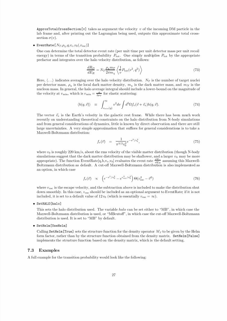
8/17/2019 Fitzpatrick 1308.6288v1


ApproxTotalCrossSection[v] takes as argument the velocity v of the incoming DM particle in thelab frame and, after printing out the Lagrangian being used, outputs this approximate total cross-section σ(v).

• EventRate[N T ,ρχ,q ,ve,v0(,vesc)]

One can determine the total detector event rate (per unit time per unit detector mass per unit recoil

energy) in terms of the transition probability P tot. One simply multiplies P tot by the appropriateprefactor and integrates over the halo velocity distribution, as follows:

dRD

dE R= N T

ρχmT

2πmχ

1

vP tot(v2, q 2)

(73)

Here, . . . indicates averaging over the halo velocity distribution. N T is the number of target nucleiper detector mass, ρχ is the local dark matter density, mχ is the dark matter mass, and mN is thenucleon mass. In general, the halo average integral should include a lower-bound on the magnitude of the velocity at vmin, which is vmin = q

2µT for elastic scattering:

h(q, v) ≡ ∞

vmin(q)

v2dv

d2Ωf v(v + ve)h(q, v). (74)

The vector ve is the Earth’s velocity in the galactic rest frame. While there has been much workrecently on understanding theoretical constraints on the halo distribution from N-body simulationsand from general considerations of dynamics, little is known by direct observation and there are stilllarge uncertainties. A very simple approximation that suffices for general considerations is to take aMaxwell-Boltzmann distribution:

f v (v) = 1

π3/2v30

e−v2/v20 , (75)

where v0 is roughly 220 km/s, about the rms velocity of the visible matter distribution (though N-bodysimulations suggest that the dark matter distribution may be shallower, and a larger v0 may be moreappropriate). The function EventRate[q,b,ve,v0] evaluates the event rate dRD

dE Rassuming this Maxwell-

Boltzmann distribution as default. A cut-off Maxwell-Boltzmann distribution is also implemented as

an option, in which case

f v(v) ∝

e−v2/v20 − ev2

esc/v2

0

Θ(v2

esc − v2) (76)

where vesc is the escape velocity, and the subtraction above is included to make the distribution shutdown smoothly. In this case, vesc should be included as an optional argument to EventRate; if it is notincluded, it is set to a default value of 12v0 (which is essentially vesc = ∞).

• SetHALO[halo]

This sets the halo distribution used. The variable halo can be set either to “MB”, in which case theMaxwell-Boltzmann distribution is used, or “MBcutoff”, in which case the cut-off Maxwell-Boltzmanndistribution is used. It is set to “MB” by default.

• SetHelm[UseHelm]

Calling SetHelm[True] sets the structure function for the density operator M J to be given by the Helmform factor, rather than by the structure function obtained from the density matrix. SetHelm[False]

implements the structure function based on the density matrix, which is the default setting.

7.3 Examples

A full example for the transition probability would look like the following:

27

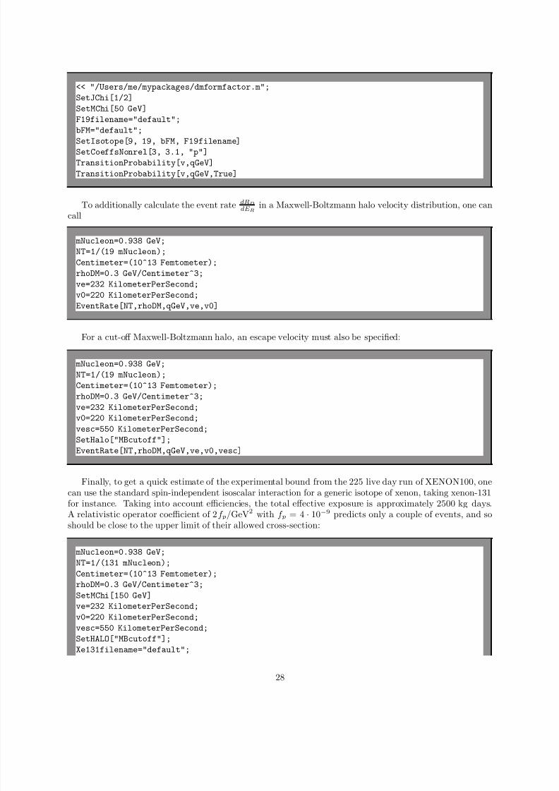
8/17/2019 Fitzpatrick 1308.6288v1


<< "/Users/me/mypackages/dmformfactor.m";

SetJChi[1/2]

SetMChi[50 GeV]

F19filename="default";

bFM="default";

SetIsotope[9, 19, bFM, F19filename]SetCoeffsNonrel[3, 3.1, "p"]

TransitionProbability[v,qGeV]

TransitionProbability[v,qGeV,True]

To additionally calculate the event rate dRD

dE Rin a Maxwell-Boltzmann halo velocity distribution, one can

call

mNucleon=0.938 GeV;

NT=1/(19 mNucleon);

Centimeter=(10^13 Femtometer);

rhoDM=0.3 GeV/Centimeter^3;ve=232 KilometerPerSecond;

v0=220 KilometerPerSecond;

EventRate[NT,rhoDM,qGeV,ve,v0]

For a cut-off Maxwell-Boltzmann halo, an escape velocity must also be specified:

mNucleon=0.938 GeV;

NT=1/(19 mNucleon);


rhoDM=0.3 GeV/Centimeter^3;

ve=232 KilometerPerSecond;

v0=220 KilometerPerSecond;vesc=550 KilometerPerSecond;

SetHalo["MBcutoff"];

EventRate[NT,rhoDM,qGeV,ve,v0,vesc]

Finally, to get a quick estimate of the experimental bound from the 225 live day run of XENON100, onecan use the standard spin-independent isoscalar interaction for a generic isotope of xenon, taking xenon-131for instance. Taking into account efficiencies, the total effective exposure is approximately 2500 kg days.A relativistic operator coefficient of 2f p/GeV2 with f p = 4 · 10−9 predicts only a couple of events, and soshould be close to the upper limit of their allowed cross-section:

mNucleon=0.938 GeV;NT=1/(131 mNucleon);


rhoDM=0.3 GeV/Centimeter^3;

SetMChi[150 GeV]

ve=232 KilometerPerSecond;

v0=220 KilometerPerSecond;

vesc=550 KilometerPerSecond;

SetHALO["MBcutoff"];

Xe131filename="default";

28

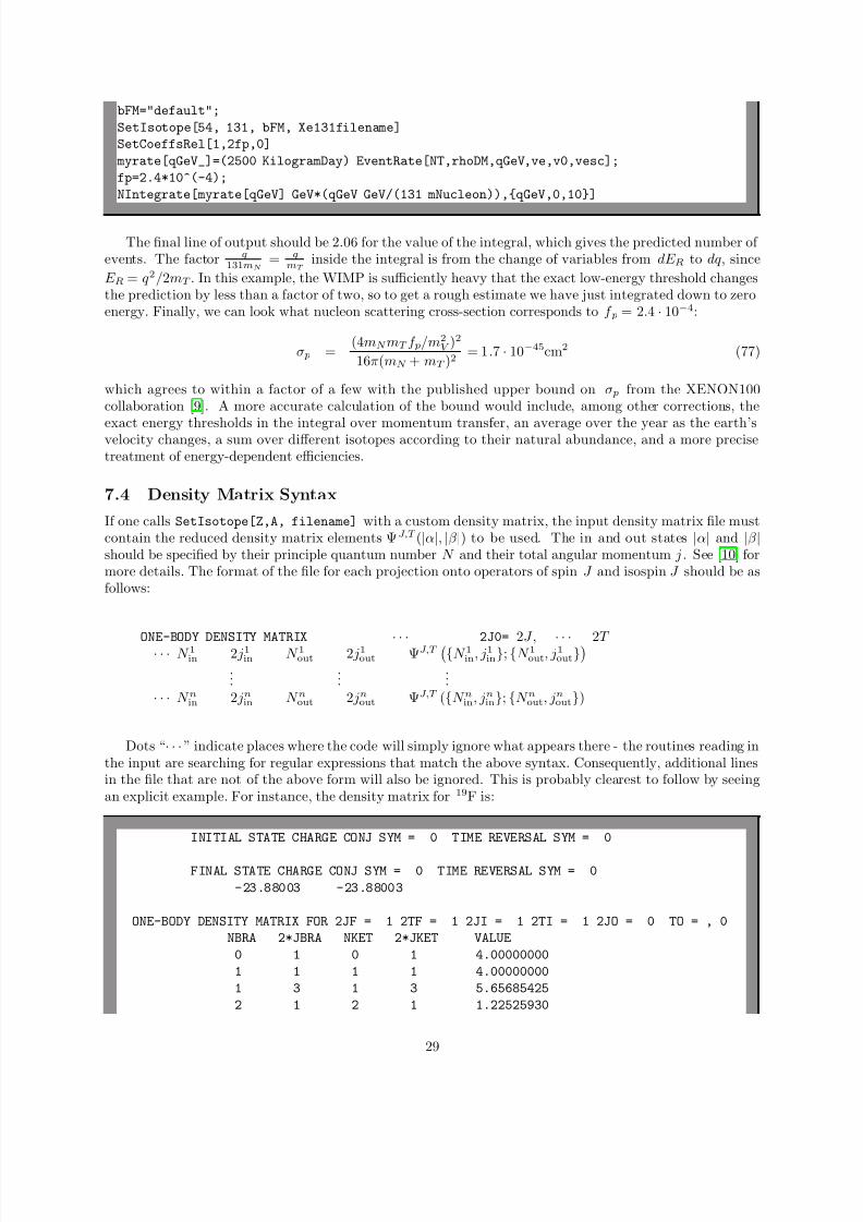
8/17/2019 Fitzpatrick 1308.6288v1


bFM="default";

SetIsotope[54, 131, bFM, Xe131filename]

SetCoeffsRel[1,2fp,0]

myrate[qGeV_]=(2500 KilogramDay) EventRate[NT,rhoDM,qGeV,ve,v0,vesc];

fp=2.4*10^(-4);

NIntegrate[myrate[qGeV] GeV*(qGeV GeV/(131 mNucleon)),qGeV,0,10]

The final line of output should be 2.06 for the value of the integral, which gives the predicted number of events. The factor q

131mN = q

mT inside the integral is from the change of variables from dE R to dq , since

E R = q 2/2mT . In this example, the WIMP is sufficiently heavy that the exact low-energy threshold changesthe prediction by less than a factor of two, so to get a rough estimate we have just integrated down to zeroenergy. Finally, we can look what nucleon scattering cross-section corresponds to f p = 2.4 · 10−4:

σ p = (4mN mT f p/m2

V )2

16π(mN + mT )2 = 1.7 · 10−45cm2 (77)

which agrees to within a factor of a few with the published upper bound on σ p from the XENON100collaboration [9]. A more accurate calculation of the bound would include, among other corrections, the

exact energy thresholds in the integral over momentum transfer, an average over the year as the earth’svelocity changes, a sum over different isotopes according to their natural abundance, and a more precisetreatment of energy-dependent efficiencies.

7.4 Density Matrix Syntax

If one calls SetIsotope[Z,A, filename] with a custom density matrix, the input density matrix file mustcontain the reduced density matrix elements ΨJ,T (|α|, |β |) to be used. The in and out states |α| and |β |should be specified by their principle quantum number N and their total angular momentum j . See [10] formore details. The format of the file for each projection onto operators of spin J and isospin J should be asfollows:

ONE-BODY DENSITY MATRIX · · · 2J0= 2J , · · · 2T · · · N 1in 2 j1in N 1out 2 j1

out ΨJ,T N 1in, j1

in; N 1out, j1out

...

......

· · · N nin 2 jnin N nout 2 jn

out ΨJ,T (N nin, jnin; N nout, jn

out)

Dots “· · · ” indicate places where the code will simply ignore what appears there - the routines reading inthe input are searching for regular expressions that match the above syntax. Consequently, additional linesin the file that are not of the above form will also be ignored. This is probably clearest to follow by seeingan explicit example. For instance, the density matrix for 19F is:

INITIAL STATE CHARGE CONJ SYM = 0 TIME REVERSAL SYM = 0

FINAL STATE CHARGE CONJ SYM = 0 TIME REVERSAL SYM = 0

-23.88003 -23.88003

ONE-BODY DENSITY MATRIX FOR 2JF = 1 2TF = 1 2JI = 1 2TI = 1 2JO = 0 TO = , 0

NBRA 2*JBRA NKET 2*JKET VALUE

0 1 0 1 4.00000000

1 1 1 1 4.00000000

1 3 1 3 5.65685425

2 1 2 1 1.22525930

29

8/17/2019 Fitzpatrick 1308.6288v1


2 3 2 3 0.20366116

2 5 2 5 0.85835832



2 1 2 1 0.36984837

2 3 2 3 0.047943792 5 2 5 0.32467225



2 1 2 1 0.44514263

2 3 2 1 -0.01197751

2 1 2 3 0.01197751

2 3 2 3 -0.05428837

2 5 2 3 -0.12172578

2 3 2 5 0.12172578

2 5 2 5 0.12280637

ONE-BODY DENSITY MATRIX FOR 2JF = 1 2TF = 1 2JI = 1 2TI = 1 2JO = 2 TO = , 2NBRA 2*JBRA NKET 2*JKET VALUE

2 1 2 1 -0.40780345

2 3 2 1 -0.01278520

2 1 2 3 0.01278520

2 3 2 3 0.01209672

2 5 2 3 0.10547489

2 3 2 5 -0.10547489

2 5 2 5 -0.24110544

Example density matrix file shown for 19 F. The density matrices for 19 F, 23 Na, 70 Ge, 72 Ge,73Ge,74Ge,76Ge,127I, 128Xe,129Xe,130Xe,131Xe,132Xe,134Xe, and 136Xe are already built into the program and no external file

is needed.

Acknowledgments

We would like to acknowledge useful conversations and feedback on the program and draft from SpencerChang, Tim Cohen, Eugenio Del Nobile, Paddy Fox, Ami Katz, and Tim Tait. NA thanks the UC Mul-tiCampus Research Program ‘Dark Matter Search Initiative’ for support. ALF was partially supported byERC grant BSMOXFORD no. 228169. WH is supported by the US Department of Energy under contractsDE-SC00046548 and DE-AC02-98CH10886.

30

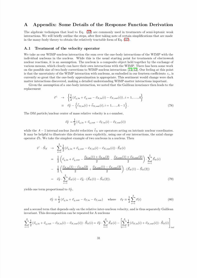
8/17/2019 Fitzpatrick 1308.6288v1


A Appendix: Some Details of the Response Function Derivation

The algebraic techniques that lead to Eq. (37) are commonly used in treatments of semi-leptonic weakinteractions. We will briefly outline the steps, after first taking note of certain simplifications that are madein the many-body theory to obtain the relatively tractable form of Eq. (37).

A.1 Treatment of the velocity operatorWe take as our WIMP-nucleus interaction the sum over the one-body interactions of the WIMP with theindividual nucleons in the nucleus. While this is the usual starting point for treatments of electroweaknuclear reactions, it is an assumption. The nucleon is a composite object held together by the exchange of various mesons, which clearly can have their own interactions with the WIMP. There has been some workon the possible size of two-body corrections to WIMP-nucleus interactions [11, 12]. Our feeling at this pointis that the uncertainty of the WIMP interaction with nucleons, as embodied in our fourteen coefficients ci, iscurrently so great that the one-body approximation is appropriate. This sentiment would change were darkmatter interactions discovered, making a detailed understanding WIMP-matter interactions important.

Given the assumption of a one-body interaction, we noted that the Galilean invariance then leads to thereplacement

v⊥ → 1

2 (vχ,in + vχ,out − vN,in(i) − vN,out(i)) , i = 1,....,A

≡ v⊥T −

vN,in(i) + vN,out(i), i = 1,...,A − 1

. (78)

The DM particle/nuclear center of mass relative velocity is a c-number,

v⊥T = 1

2 (vχ,in + vχ,out − vT,in(i) − vT,out(i))

while the A − 1 internal nuclear Jacobi velocities vN are operators acting on intrinsic nuclear coordinates.It may be helpful to illustrate this division more explicitly, using one of our interactions, the axial chargeoperator O7. We take the simplest example of two nucleons in a nucleus. Then

v⊥ · S N →2

i=1

12

(vχ,in + vχ,out − vN,in(i) − vN,out(i)) · S N (i)

= 1

2

vχ,in + vχ,out − vN,in(1) + vN,in(2)

2 − vN,out(1) + vN,out(2)

2

·

2i=1

S N (i)

− 1

2

vN,in(1) − vN,in(2)

2 +

vN,out(1) − vN,out(2)

2

· ( S N (1) − S N (2))

= v⊥T ·2

i=1

S N (i) − v⊥N · ( S N (1) − S N (2)). (79)

yields one term proportional to v⊥T ,

v⊥T ≡ 1

2 (vχ,in + vχ,out − vT,in − vT,out) where vT ≡ 1

2

2i=1

v(i) (80)

and a second term that depends only on the relative inter-nucleon velocity, and is thus separately Galileaninvariant. This decomposition can be repeated for A nucleons

Ai=1

1

2 (vχ,in + vχ,out − vN,in(i) − vN,out(i)) · S N (i) = v⊥T ·

Ai=1

S N (i) −

Ai=1

1

2 (vN,in(i) + vN,out(i)) · S N (i)

int

31

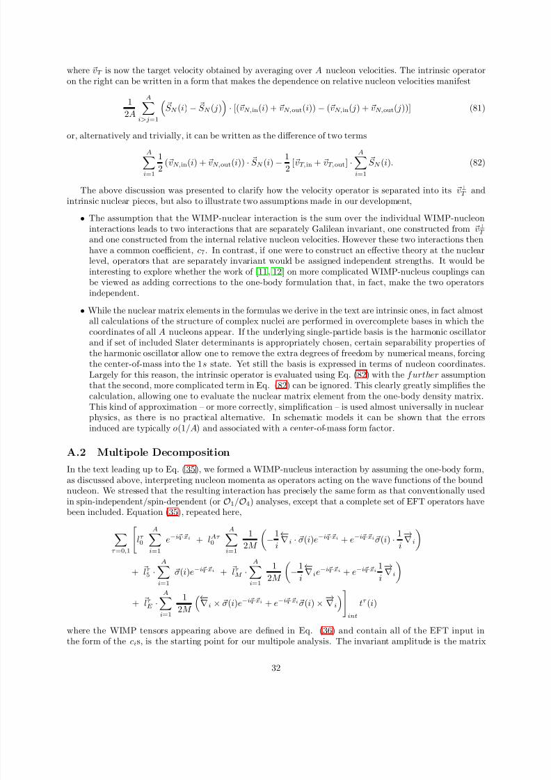
8/17/2019 Fitzpatrick 1308.6288v1


where vT is now the target velocity obtained by averaging over A nucleon velocities. The intrinsic operatoron the right can be written in a form that makes the dependence on relative nucleon velocities manifest

1

2A

Ai>j=1

S N (i) − S N ( j)

· [(vN,in(i) + vN,out(i)) − (vN,in( j) + vN,out( j))] (81)

or, alternatively and trivially, it can be written as the difference of two termsA

i=1

1

2 (vN,in(i) + vN,out(i)) · S N (i) − 1

2 [vT,in + vT,out] ·

Ai=1

S N (i). (82)

The above discussion was presented to clarify how the velocity operator is separated into its v⊥T andintrinsic nuclear pieces, but also to illustrate two assumptions made in our development,

• The assumption that the WIMP-nuclear interaction is the sum over the individual WIMP-nucleoninteractions leads to two interactions that are separately Galilean invariant, one constructed from v⊥T

and one constructed from the internal relative nucleon velocities. However these two interactions thenhave a common coefficient, c7. In contrast, if one were to construct an effective theory at the nuclearlevel, operators that are separately invariant would be assigned independent strengths. It would be

interesting to explore whether the work of [11, 12] on more complicated WIMP-nucleus couplings canbe viewed as adding corrections to the one-body formulation that, in fact, make the two operatorsindependent.

• While the nuclear matrix elements in the formulas we derive in the text are intrinsic ones, in fact almostall calculations of the structure of complex nuclei are performed in overcomplete bases in which thecoordinates of all A nucleons appear. If the underlying single-particle basis is the harmonic oscillatorand if set of included Slater determinants is appropriately chosen, certain separability properties of the harmonic oscillator allow one to remove the extra degrees of freedom by numerical means, forcingthe center-of-mass into the 1s state. Yet still the basis is expressed in terms of nucleon coordinates.Largely for this reason, the intrinsic operator is evaluated using Eq. (82) with the f urther assumptionthat the second, more complicated term in Eq. (82) can be ignored. This clearly greatly simplifies thecalculation, allowing one to evaluate the nuclear matrix element from the one-body density matrix.

This kind of approximation – or more correctly, simplification – is used almost universally in nuclearphysics, as there is no practical alternative. In schematic models it can be shown that the errorsinduced are typically o(1/A) and associated with a center-of-mass form factor.

A.2 Multipole Decomposition

In the text leading up to Eq. (35), we formed a WIMP-nucleus interaction by assuming the one-body form,as discussed above, interpreting nucleon momenta as operators acting on the wave functions of the boundnucleon. We stressed that the resulting interaction has precisely the same form as that conventionally usedin spin-independent/spin-dependent (or O1/O4) analyses, except that a complete set of EFT operators havebeen included. Equation (35), repeated here,

τ =0,1

lτ 0

A

i=1

e−i q·xi + lAτ 0

A

i=1

1

2M −

1

i

←−∇

i

·σ(i)e−i q·xi + e−i q·xiσ(i)

· 1

i

−→∇

i+ lτ

5 ·A

i=1

σ(i)e−i q·xi + lτ M ·

Ai=1

1

2M

−1

i

←−∇ie−i q·xi + e−i q·xi 1

i

−→∇i

+ lτ E ·

Ai=1

1

2M

←−∇i × σ(i)e−i q· xi + e−i q·xiσ(i) × −→∇i

int

tτ (i)

where the WIMP tensors appearing above are defined in Eq. (36) and contain all of the EFT input inthe form of the cis, is the starting point for our multipole analysis. The invariant amplitude is the matrix

32

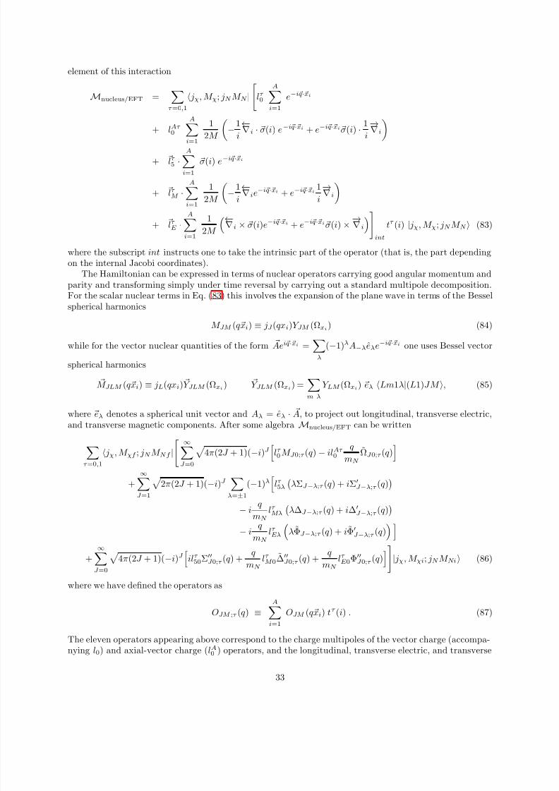
8/17/2019 Fitzpatrick 1308.6288v1


element of this interaction

Mnucleus/EFT =

τ =0,1

jχ, M χ; jN M N |

lτ 0

Ai=1

e−i q·xi

+ lAτ 0

A

i=1

1

2M −

1

i

←−∇

i

·σ(i) e−i q·xi + e−i q·xiσ(i)

· 1

i

−→∇

i+ lτ

5 ·A

i=1

σ(i) e−i q·xi

+ lτ M ·

Ai=1

1

2M

−1

i

←−∇ie−i q·xi + e−i q·xi 1

i

−→∇ i

+ lτ E ·

Ai=1

1

2M

←−∇i × σ(i)e−i q·xi + e−i q·xiσ(i) × −→∇ i

int

tτ (i) | jχ, M χ; jN M N (83)

where the subscript int instructs one to take the intrinsic part of the operator (that is, the part dependingon the internal Jacobi coordinates).

The Hamiltonian can be expressed in terms of nuclear operators carrying good angular momentum andparity and transforming simply under time reversal by carrying out a standard multipole decomposition.For the scalar nuclear terms in Eq. (83) this involves the expansion of the plane wave in terms of the Besselspherical harmonics

M JM (qxi) ≡ jJ (qxi)Y JM (Ωxi) (84)

while for the vector nuclear quantities of the form Aei q·xi =

λ

(−1)λA−λeλe−i q·xi one uses Bessel vector

spherical harmonics

M JLM (qxi) ≡ jL(qxi) Y JLM (Ωxi) Y JLM (Ωxi) =m λ

Y LM (Ωxi) eλ Lm1λ|(L1)JM , (85)

where eλ denotes a spherical unit vector and Aλ = eλ · A, to project out longitudinal, transverse electric,and transverse magnetic components. After some algebra Mnucleus/EFT can be written

τ =0,1

jχ, M χf ; jN M N f | ∞

J =0

4π(2J + 1)(−i)J

lτ

0 M J 0;τ (q ) − ilAτ 0

q

mN ΩJ 0;τ (q )

+∞

J =1

2π(2J + 1)(−i)J

λ=±1

(−1)λ

lτ 5λ

λΣJ −λ;τ (q ) + iΣ′

J −λ;τ (q )

− i q

mN lτ

Mλ

λ∆J −λ;τ (q ) + i∆′

J −λ;τ (q )

− i q

mN lτ

Eλ

λΦJ −λ;τ (q ) + iΦ′

J −λ;τ (q )

+ ∞J =0

4π(2J + 1)(−i)J

ilτ

50Σ′′J 0;τ (q ) + q

mN lτ

M 0 ∆′′J 0;τ (q ) + q

mN lτ

E 0Φ′′J 0;τ (q )

| jχ, M χi; jN M Ni (86)

where we have defined the operators as

OJM ;τ (q ) ≡A

i=1

OJM (qxi) tτ (i) . (87)

The eleven operators appearing above correspond to the charge multipoles of the vector charge (accompa-nying l0) and axial-vector charge (lA

0 ) operators, and the longitudinal, transverse electric, and transverse

33

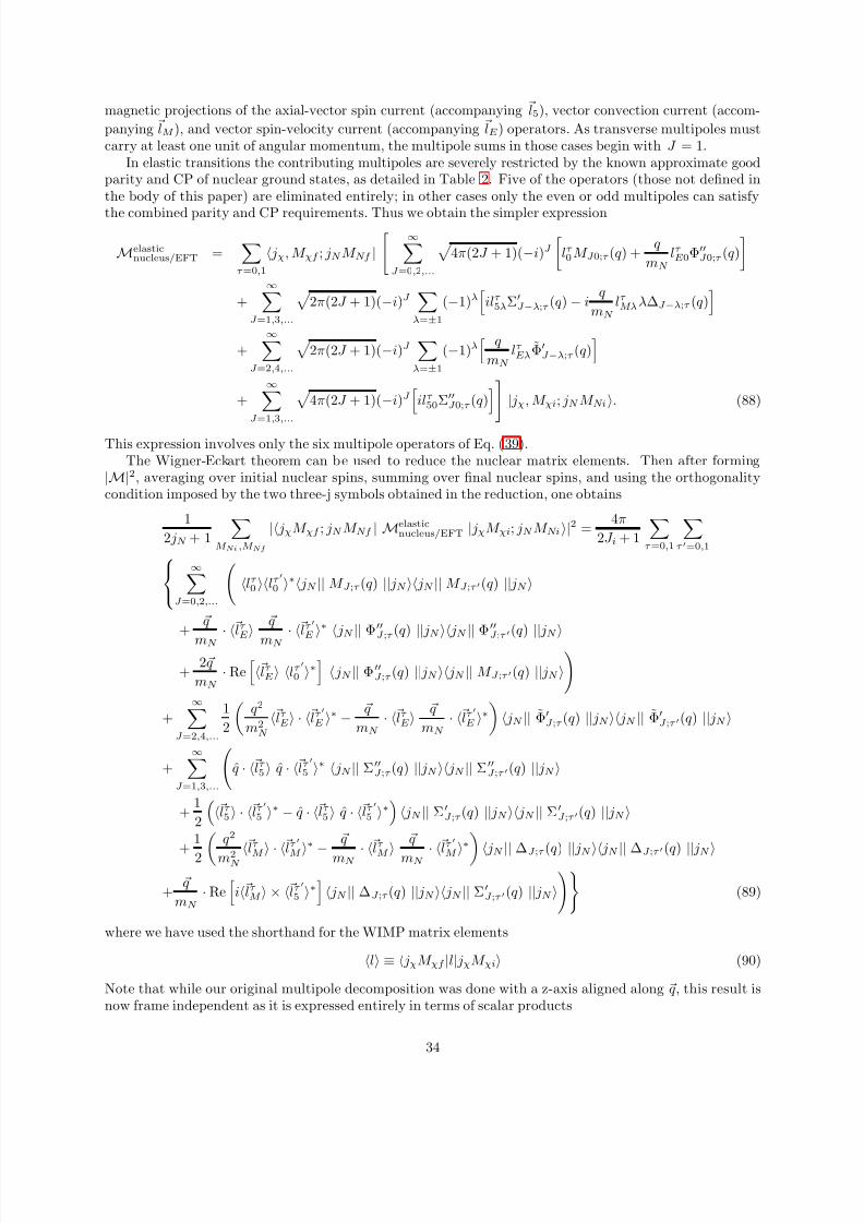
8/17/2019 Fitzpatrick 1308.6288v1


magnetic projections of the axial-vector spin current (accompanying l5), vector convection current (accom-

panying lM ), and vector spin-velocity current (accompanying lE ) operators. As transverse multipoles mustcarry at least one unit of angular momentum, the multipole sums in those cases begin with J = 1.

In elastic transitions the contributing multipoles are severely restricted by the known approximate goodparity and CP of nuclear ground states, as detailed in Table 2. Five of the operators (those not defined inthe body of this paper) are eliminated entirely; in other cases only the even or odd multipoles can satisfy

the combined parity and CP requirements. Thus we obtain the simpler expression

Melasticnucleus/EFT =

τ =0,1

jχ, M χf ; jN M Nf | ∞

J =0,2,...

4π(2J + 1)(−i)J

lτ

0 M J 0;τ (q ) + q

mN lτ

E 0Φ′′J 0;τ (q )

+

∞J =1,3,...

2π(2J + 1)(−i)J

λ=±1

(−1)λ

ilτ 5λΣ′

J −λ;τ (q ) − i q

mN lτ

Mλ λ∆J −λ;τ (q )

+

∞J =2,4,...

2π(2J + 1)(−i)J

λ=±1

(−1)λ q

mN lτ

EλΦ′J −λ;τ (q )

+∞

J =1,3,... 4π(2J + 1)(−i)J

ilτ

50Σ′′J 0;τ (q )

| jχ, M χi; jN M Ni. (88)

This expression involves only the six multipole operators of Eq. (39).The Wigner-Eckart theorem can be used to reduce the nuclear matrix elements. Then after forming

|M|2, averaging over initial nuclear spins, summing over final nuclear spins, and using the orthogonalitycondition imposed by the two three-j symbols obtained in the reduction, one obtains

1

2 jN + 1

M Ni ,M Nf

| jχM χf ; jN M Nf | Melasticnucleus/EFT | jχM χi; jN M Ni|2 =

4π

2J i + 1

τ =0,1

τ ′=0,1

∞

J =0,2,...

lτ

0 lτ ′

0 ∗ jN || M J ;τ (q ) || jN jN || M J ;τ ′(q ) || jN

+ q

mN · lτ

E

q

mN · lτ ′

E

∗

jN

|| Φ′′

J ;τ (q )

|| jN

jN

|| Φ′′

J ;τ ′(q )

|| jN

+

2 q

mN · Re

lτ

E lτ ′

0 ∗ jN || Φ′′

J ;τ (q ) || jN jN || M J ;τ ′(q ) || jN

+∞

J =2,4,...

1

2

q 2

m2N

lτ E · lτ ′

E ∗ − q

mN · lτ

E q

mN · lτ ′

E ∗

jN || Φ′J ;τ (q ) || jN jN || Φ′

J ;τ ′(q ) || jN

+∞

J =1,3,...

q · lτ

5 q · lτ ′

5 ∗ jN || Σ′′J ;τ (q ) || jN jN || Σ′′

J ;τ ′(q ) || jN

+ 1

2

lτ

5 · lτ ′

5 ∗ − q · lτ 5 q · lτ ′

5 ∗

jN || Σ′J ;τ (q ) || jN jN || Σ′

J ;τ ′(q ) || jN

+ 1

2 q 2

m2N lτ

M · lτ ′

M ∗

− q

mN · lτ

M q

mN · lτ ′

M ∗

jN

|| ∆J ;τ (q )

|| jN

jN

|| ∆J ;τ ′(q )

|| jN

+

q

mN · Re

i lτ

M × lτ ′

5 ∗ jN || ∆J ;τ (q ) || jN jN || Σ′

J ;τ ′(q ) || jN

(89)

where we have used the shorthand for the WIMP matrix elements

l ≡ jχM χf |l| jχM χi (90)

Note that while our original multipole decomposition was done with a z-axis aligned along q , this result isnow frame independent as it is expressed entirely in terms of scalar products

34

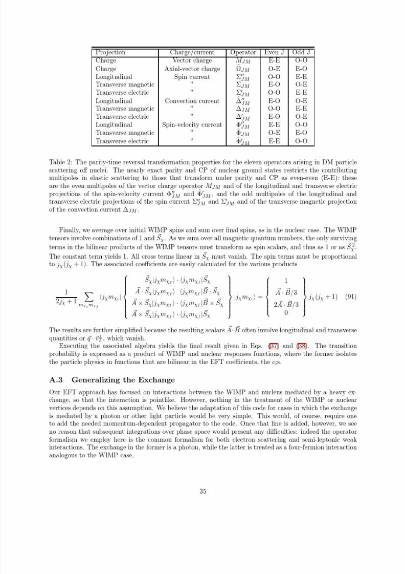
8/17/2019 Fitzpatrick 1308.6288v1


8/17/2019 Fitzpatrick 1308.6288v1


References

[1] A. L. Fitzpatrick, W. C. Haxton, E. Katz, N. Lubbers, and Y. Xu, JCAP 004, 1302 (2013),(arXiv:1203.3542).

[2] K. Freese, M. Lisanti, and C. Savage, to appear in Rev. Mod. Phys (2013), (arXiv:1209.3339).

[3] G. Bertone, D. Hooper, and J. Silk, Phys. Reports 405, 279 (2005), (arXiv:hep-ph/0404175).

[4] M. W. Goodman and E. Witten, Phys. Rev. D 31, 3059 (1985).

[5] A. K. Drukier, K. Freese, and D. N. Spergel, Phys. Rev. D 33, 3495 (1986).

[6] G. Jungman, M. Kamionkowski, and K. Griest, Phys. Repts. 267, 195 (1996), (arXiv:hep-ph/9506380).

[7] J. Fan, M. Reece, and L.-T. Wang, JCAP 11, 042 (2010), (arXiv:1008.1591).

[8] T. Donnelly and W. Haxton, Atomic Data and Nuclear Data Tables 23, 103 (1979).

[9] XENON100 Collaboration, E. Aprile et al., Phys. Rev. Lett. 109, 181301 (2012), (arXiv:1207.5988).

[10] W. Haxton and C. Lunardini, Comp. Phys. Comm. 179, 345 (2008), (arXiv:0706.2210).

[11] V. Cirigliano, M. Graesser, and G. Ovanesyan, JHEP 10, 025 (2012), (arXiv:1205.2695).

[12] J. Menendez, D. Gazit, and A. Schwenk, Phys. Rev. D 86, 103511 (2012), (arXiv:1208.1094).

Fitzpatrick 1308.6288v1

Documents

Transcript of Fitzpatrick 1308.6288v1