Massachusetts Division of Fisheries and Wildlife University of
FISHERIES DIVISION
RESEARCH REPORT Number 2029 July 30, 1996
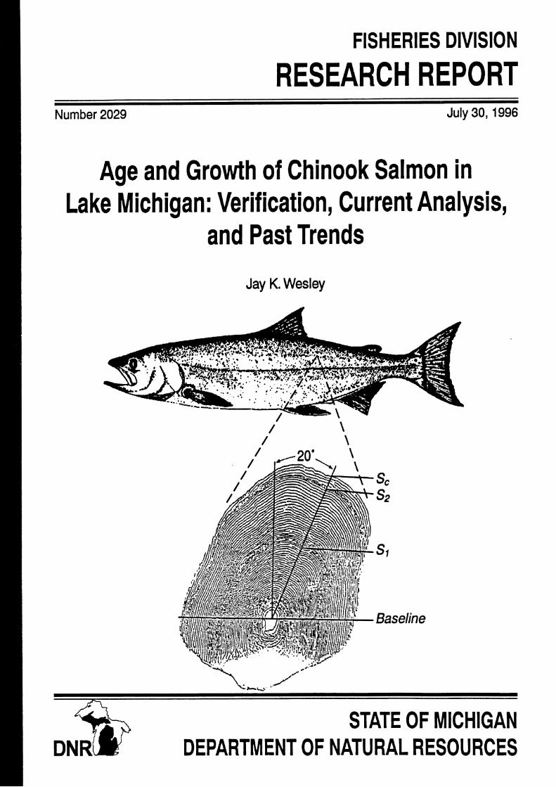
Age and Growth of Chinook Salmon in Lake Michigan: Verification, Current Analysis,
and Past Trends
Jay K. Wesley
Baseline
STATE OF MICHIGAN C D oF NATURAL RESOURCES

MICHIGAN DEPARTMENT OF NATURAL RESOURCES FISHERIES DIVISION
Fisheries Research Report 2029 July 30,1996
AGE AND GROWTH OF CHINOOK SALMON IN LAKE MICHIGAN: VERIFICATION, CURRENT ANALYSIS, AND PAST TRENDS
Jay K. Wesley
Ibe Michigan Department of Natunl Resources, (MDNR) pv ided equal opportunities f a employment uid for access t~ Michigan's natural resouras. State uid Fedenl hwsprohibitdiPcrimhtionoa the basis o f n a , cola, sex, m t i d migin, religion, dislbili~,age,mlvilrrlsuhls,heightmd weight If you believe that you have been discriminated against in any pgnm, adivity or facility, pkaac write the MDNR Equal Opportunity ma, P.O. Box 30028, Lansing, M148909, or the Michigan Deprtment of Civil R i g h 12006lhAvenue, Detroit, MI 48226, or the ma of Hurmn R e s o w , U.S. Fiuid Wildlife Service, Washington D.C 20204. For more information about this publiatioaa theAmerianhbiiitiesAd(ADA), watrd, Michigan Deprimcnt of Natunl Resources, Fisheries Division, Box 30446, k i n g , MI 48909, a all 517-373-1280.
TOTAL UNITS PRINTED: 300; TOTAL PRINTING COST: 51,211.36; COST PER UNIT: $4.03

AGE AND GROWTH OF CHINOOK SALMON IN LAKE MICHIGAN:
VERIFICATION, CURRENT ANALYSIS, AND PAST TRENDS
by
Jay K. Wesley
A thesis submitted in partial fulfillment
of the requirements for the degree of
Masters of Science
School of Natural Resources and Environment
The University of Michigan
1996
Committee members
Associate Professor James S. Diana, chairman
Adjunct Assistant Professor Richard D. Clark, Jr.

ABSTRACT
Chinook salmon Oncorhynchus tshawytscha from the Lake Michigan sport
fishery were studied to determine if changes in age and growth occurred with recent
forage shifts from alewife Alosa pseudoharengus to bloater chub Coregonus hoyi. A
decrease in growth may indicate that forage shift stress caused the outbreak of
bacterial kidney disease (BKD) Renibacterium salmoninarum. Known age chinook
salmon implanted with coded-wire tags were collected in 1994 to validate aging
techniques and to compare growth between fish collected by anglers and gill nets.
Scale and vertebra aging were 95.6% and 93.9% accurate, respectively. There were
no differences in age, gender, and maturity specific mean back calculated lengths
(mm) between harvest gears. There was also no difference in mean back calculated
length between sexes; however, immature age-0.2 fish were smaller than mature age-
0.2 fish. Mean back calculated total lengths and Fulton Indices of condition were
used to analyze historic growth using data and scales from the Michigan Department
of Natural Resources Lake Michigan Creel Survey from 1983 to 1993. Average age
decreased from a high in 1986 of 2.59 years to a low of 1.53 years in 1993. Mean
length and condition declined recently for age 0.1. Mean length increased from 1983
to 1993 for age 0.3. Condition increased after BKD for age 0.3 and 0.4 chinook
salmon. The increase in length and condition of age 0.3 and 0.4 chinook salmon may
be a competitive release andtor size differential mortality in response to BKD. A
reduction of chinook salmon stocking in Lake Michigan might restore growth and
reduce mortality associated with BKD.

ACKNOWLEDGMENTS
Funding for this project was provided by a grant from the National Oceanic
and Atmospheric Administration award number NA56FA05 14, the Michigan
Department of Natural Resources under Fisheries Division Study 479, and the
University of Michigan.
I would like to thank my major professor Jim Diana for accepting me as a
student as well as for his support, guidance, and patience. His willingness to always
make time for students is much appreciated. I would also like to thank Rick Clark for
serving on my committee and also for his work funding this project. Kelley Smith
was also very instrumental in getting this project funded and off the ground.
I wish to acknowledge everyone at the Institute for Fisheries Research,
especially Jim Schneider, for office space and support. Jim Gapczynski helped
tremendously with equipment and making slides. Marlene Reynolds and Barb
Champion gave secretarial support, and A1 Sutton provided field transportation and
computer support. Paul Seelbach, Jim Breck, Ed Rutherford, and Roger Lockwood
gave useful comments and suggestions towards this project.
I also wish to thank the personnel at the Charlevoix Fisheries Station,
especially Myrl Keller for equipment and supplies and Jerry Rakoczy for use of creel
survey data and scales. John Clevenger, Paul Gelderblom, and Donna Wesander
processed coded-wire tags and provided vertebra information. Ron Svoboda
unselfishly gave a great deal of phone time discussing techques for scale aging
chinook salmon.

I thank Rob Elliott and Jay Hesse for giving me the opportunity to work with
them and for increasing my knowledge of chinook salmon in Lake Michigan. I also
want to thank Rob Elliott and Bruce Peffers for their companionship and volunteering
efforts in the field. I wish to recognize Dan Hayes and Michigan State University for
lodging during my field season in 1994. The "attic rats" (Kevin Wehrly, Sarah Zorn,
Aaron Woldt, Michele DePhilip, and Dave Swank) all answered several of my
questions and made my time at the University of Michigan very enjoyable.
Finally, I would like to thank my entire family, especially my parents Mike and
Joyce as well as my brother Rob and sister Marti for their understanding,
encouragement, and support, I am also very grateful to my fiancee Jill and her family.
Jill gave unlimited emotional support and presented great patience. She was my
inspiration during this educational experience.

TABLE OF CONTENTS
Page
. . . . . . . . . . . . . . . . . . . . . . . . . . . . . . . . . . . . . . . . . . . . . . . . . . . . List of Tables vii
. . . . . . . . . . . . . . . . . . . . . . . . . . . . . . . . . . . . . . . . . . . . . . . . . . . . List of Figures ix
. . . . . . . . . . . . . . . . . . . . . . . . . . . . . . . . . . . . . . . . . . . Chapter One. Introduction 1
Chapter Two. The Development and Validation of an Accurate Aging Technique . . . . . . . . . . . . . . . . . . . . . . . . . . for Chinook Salmon from Lake Michigan 6
. . . . . . . . . . . . . . . . . . . . . . . . . . . . . . . . . . . . . . . . . . . . . . . . Introduction 6
. . . . . . . . . . . . . . . . . . . . . . . . . . . . . . . . . . . . . . . . . . . . . . . . . . . Methods 7
. . . . . . . . . . . . . . . . . . . . . . . . . . . . . . . . . . . . . . . . . Sample Source 7
. . . . . . . . . . . . . . . . . . . . . . . . . . . . . . . . . . Laboratory Preparation 8
. . . . . . . . . . . . . . . . . . Accuracy and Precision Estimates for Scales 15
Results . . . . . . . . . . . . . . . . . . . . . . . . . . . . . . . . . . . . . . . . . . . . . . . . . . . 18
. . . . . . . . . . . . . . . . . . . . . . . . . . . . . . . . . . Accuracy and Precision 19
. . . . . . . . . . . . . . . . . . . . . . . . . . . . . . . . . . . . . . . . . . . . . . . . . Discussion 26
Chapter Three. Growth Rate by Age. Sex. and Maturity Classes of Chinook . . . . . . . . . . . . . . . . . . . . . . . . . . . . . . . . . . . . . Salmon in Lake Michigan 36
Introduction . . . . . . . . . . . . . . . . . . . . . . . . . . . . . . . . . . . . . . . . . . . . . . . 36
. . . . . . . . . . . . . . . . . . . . . . . . . . . . . . . . . . . . . . . . . . . . . . . . . . Methods 39
Sample Source and Preparation . . . . . . . . . . . . . . . . . . . . . . . . . . . . 39
. . . . . . . . . . . . . . . . . . . . . . . . . . . . . . . . . . . . . . . Growth Analysis 41
Results . . . . . . . . . . . . . . . . . . . . . . . . . . . . . . . . . . . . . . . . . . . . . . . . . . . 44
. . . . . . . . . . . . . . . . . . . . . . . . . . . . . . . . . . . . . . . . . . . . . . . . . Discussion 49

Chapter Four. Comparison of Size at Age for Chinook Salmon in Lake . . . . . . . . . . . . . . . . . . . . . . . . . . . . . . . . . . . . . . . . Michigan. 1983- 1993 58
. . . . . . . . . . . . . . . . . . . . . . . . . . . . . . . . . . . . . . . . . . . . . . . Introduction 58
. . . . . . . . . . . . . . . . . . . . . . . . . . . . . . . . . . . . . . . . . . . . . . . . . . . Methods 59
. . . . . . . . . . . . . . . . . . . . . . . . . . . . . . . . . . . . . . . . . . . . . . . . . . . Results 62
. . . . . . . . . . . . . . . . . . . . . . . . . . . . . . . . . . . . . . . . . . . . . . . . . Discussion 73
. . . . . . . . . . . . . . . . . . . . . . . . . . . . . . . . . . . . . . . . . . . . . . . . . . . . . . AppendixA 83
. . . . . . . . . . . . . . . . . . . . . . . . . . . . . . . . . . . . . . . . . . . . . . . . . . . . . . Appendix B 84
. . . . . . . . . . . . . . . . . . . . . . . . . . . . . . . . . . . . . . . . . . . . . . . . . . . Literature Cited 85

Table
List of Tables
Page
1. Timing of annulus formation in scales of chinook salmon from Lake Michigan. Samples include coded-wire tagged chinook salmon from the 1994 sport fishery and Ludington Pumped Storage Assessment
. . . . . . . . . . . . . . . . . . . . . . . . . . . . . . . . . . . . . . . . . . . . . . . . . . . . . . gill nets . 2 0
2. The percent and number of the total collected chinook salmon (in parenthesis) . . . . . . . . . . . . . . . . . . showing scale erosion reported by age, sex, and month . 2 2
. . . . . . . . . . . . . . . . . 3. Scale aging accuracy for collected CWT chinook salmon 23
4. Differences between known age and age estimated by scales for CWT fish . . . . . . . . . . . . . . . . . . . . . . . . . . . . . . . . . . . . . . . . . . . . . . that were misaged . 2 4
5. Distribution of the percent of misaged chinook salmon scales based on . . . . . . . . . . . . . . . . . . . . . . . . . . . . . . . . . . . . . . . . . . . . maturity and gender. 25
6. Vertebra aging accuracy of collected CWT chinook salmon sampled . . . . . . . . 27
7. Differences between known age and age estimated by vertebrae for . . . . . . . . . . . . . . . . . . . . . . . . . . . . . . . . . . . . . . CWT fish that were misaged . 2 8
8. Distribution of the percent of misaged chinook salmon vertebrae based . . . . . . . . . . . . . . . . . . . . . . . . . . . . . . . . . . . . . . . . . on maturity and gender. - 2 9
9. Estimated scale ages and associated APE, V, and D of 3 readers who each analyzed scales from 76 chinook salmon taken in Lake Michigan . . . . . . . 30
10. Age and gender specific mean back calculated total lengths (mm) for CWT chinook salmon from Lake Michigan harvested anglers or gill net, 1994 . . . . . . . . . . . . . . . . . . . . . . . . . . . . . . . . . . . . . . . . . . . . . . . . . . . . . . . . 47
11. Age 0.2 gender and maturity specific mean back calculated total lengths (mm) for sport and gill net harvested chinook salmon from
. . . . . . . . . . . . . . . . . . . . . . . . . . . . . . . . . . . . . Lake Michigan, 1994
12. Pooled age, gender, and maturity (I for immature; M for mature) specific mean back calculated total lengths (rnm) for sport and gill net harvested chinook salmon from Lake Michigan , 1994 . . . . . . . . . . . . . . . . . . 50

13. Mean back calculated lengths (rnrn) at earlier age of chinook salmon from the Michigan waters of Lake Michigan based on gender and
. . . . . . . . . . . . . . . . . . . . . . . . . . . . . . . . . . . . . . . . . . . . . . . . maturity ... . 5 1
14. Proportion of the sample comprising each age class, and average age for chinook salmon from Lake Michigan (1 983- 1993). Sample sizes in parentheses . . . . . . . . . . . . . . . . . . . . . . . . . . . . . . . . . . . . . . . . . . . . . . . . .63
15. Percent of sample with one year of stream residence, or of age 0.5 fish, based on the total sample of chinook salmon each year (1983- 1993).
. . . . . . . . . . . . . . . . . . . . . . . . . . . . . . . . . . . . . . Sample sizes in parentheses 64
16. Mean back calculated length at age for chinook salmon taken by anglers in Lake Michigan from 1983 to 1993 (sample sizes in parentheses) . . . . . . . . . 65
17. Weight(@ - Length (mm) relationships for chinook salmon harvested by anglers from Michigan waters of Lake Michigan, 1983-1993. Harvest dates were between 1 April and 30 June. Evaluations were fit to
. . . . . . . . . . . . . . . . . . . . . . . . . . . . . . . . . . . . . . . Log W = Log a + b Log L 69
18. Mean back calculated weight (g) for each age of chinook salmon from Lake Michigan, 1983 to 1993 . . . . . . . . . . . . . . . . . . . . . . . . . . . . . . . . . . . . .70
19. Mean Fulton Indices for each age of chinook salmon from Lake Michigan, 1983 to 1993 . . . . . . . . . . . . . . . . . . . . . . . . . . . . . . . . . . . . . . . . . 7 1
20. Comparison of mean back calculated length (mm) and Fulton Indices (FI) for chinook salmon harvested in the northern (Ludington and north) and southern (Muskegon and south) regions of Lake Michigan before 30June . . . . . . . . . . . . . . . . . . . . . . . . . . . . . . . . . . . . . . . . . . . . . . . . . . . . . 75
2 1. Mean scale increment length (rnrn) for age 0.1 (focus to 1 st annulus), age 0.2 (1st to 2nd annulus), age 0.3 (2nd to 3rd annulus), and age 0.4 (3rd to 4th annulus) chinook salmon sport harvested from Lake Michigan, 1983- 1993 . . . . . . . . . . . . . . . . . . . . . . . . . . . . . . . . . . . . . . . . . . . . . . . . . . . . . . . . 83
22. Ford's growth equation (L+I = L, (I-k) + kL) and Brody's coefficients (K = -Ink) for creel harvested chinook salmon from Lake Michigan, 1983-1993 . . . . . . . . . . . . . . . . . . . . . . . . . . . . . . . . . . . . . . . . . . . . . . . . . . . 84

List of Figures
Figure Page
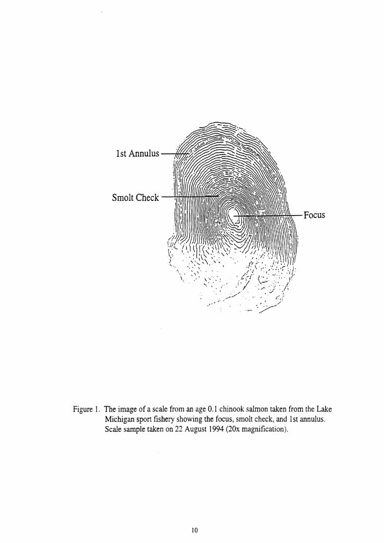
1. The image of a scale from an age 0.1 chinook salmon taken from the Lake Michigan sport fishery showing the focus, smolt check, and 1st annulus. Scale sample taken on 22 August 1994 (20x magnification) . . . . . . . . 10
2. Magnified image of an age 0.2 chinook salmon scale taken in the Lake Michigan sport fishery on 23 August 1994 (20x magnification) . . . . . . . . . . . . . 11
3. Magnified image of an age 0.3 chinook salmon scale taken in the Lake Wchigan sport fishery on 10 July 1994 (lox magnification) . . . . . . . . . . . . . . . 12
4. Magnified image of an age 0.4 chinook salmon scale taken in the Lake Michigan sport fishery on 1 June 1994 (lox magnification) . . . . . . . . . . . . . . . . 13
5. Magnified image of an age 0.1 chinook salmon scale taken in the Lake Michigan spoft fishery on 7 May 1994, with the first annulus just visible on the scale margin (20x magnification) . . . . . . . . . . . . . . . . . . . . . . . . . . . . . . 14
6. Magnified image of an age 0.2 chinook salmon scale taken in the Lake Michigan sport fishery on 27 August 1994, showing extensive erosion on the posterior margin (20x magnification) . . . . . . . . . . . . . . . . . . . . . . . . . . . 16
7. Magnified image of a severely eroded chinook salmon scale from the fall river sport fishery, 20 September 1994 (15x magnification) . . . . . . . . . . . . . . . 17
8. Percent of chinook salmon having started and completed scale annulus . . . . . . . . . . . . formation by month for fish taken from Lake Michigan in 1994 . 2 1
9. A map of Lake Michigan and location of sampled ports . . . . . . . . . . . . . . . . . . 40
10. Illustration of a chinook salmon scale with measurements used in the Fraser-Lee back calculation formula. S1 is the distance from the focus to the 1 st annulus, S2 is the distance from the focus to the 2nd annulus, and S, is the distance from the focus to the scale edge. All measurements were taken at about 20°from the perpendicular axis of the scale (20x
. . . . . . . . . . . . . . . . . . . . . . . . . . . . . . . . . . . . . . . . . . . . . magnification)
11. Plot of scale radius and fish total length for sport harvested chinook . . . . . . . . . . . . . . . . . . . . . . . . . . . . . . . . . . . salmon in Lake Michigan, 1994 . 4 5
12. Plot of scale radius and fish total length for gill netted chinook salmon in Lake Michigan, 1994. . . . . . . . . . . . . . . . . . . . . . . . . . . . . . . . . . . . 4 6

13. Lake Michigan chinook salmon back calculated yearly growth increments for females based on total lengths of the pooled sport and
. . . . . . . . . . . . . . . . . . . . . . . . . . . . . . . . . . . . . . . . . . . gill netted data, 1994 . 5 2
14. Lake Michigan chinook salmon back calculated yearly growth increments for males based on total lengths of the pooled sport and gill
. . . . . . . . . . . . . . . . . . . . . . . . . . . . . . . . . . . . . . . . . . . . . netted data, 1994. 53
15. Back calculated lengths of age 0.1 and 0.2 chinook salmon from Lake Michigan, 1983-1993. Means are represented by filled squares, brackets represent 95% confidence intervals. Sample size is below the xaxis . . . . . . . . . . . . . . . . . . . . . . . . . . . . . . . . . . . . . . . . . . . . . . . . . . . . . . . 66
16. Back calculated lengths of age 0.3 and 0.4 chinook salmon from Lake Michigan, 1983-1993. Means are represented by filled squares, brackets represent 95% confidence intervals. Sample size is below the xaxis . . . . . . . . . . . . . . . . . . . . . . . . . . . . . . . . . . . . . . . . . . . . . . . . . . . . . . . 68
17. Fulton Indices of age 0.1 and 0.2 chinook salmon from Lake Michigan, 1983-1993. Means are represented by filled squares, brackets represent 95% confidence intervals. Sample size is below the xaxis . . . . . . . . . . . . . . . . . . . . . . . . . . . . . . . . . . . . . . . . . . . . . . . . . . . . . . . 72
18. Fulton Indices of age 0.3 and 0.4 chinook salmon from Lake Michigan, 1983-1993. Means are represented by filled squares, brackets represent 95% confidence intervals. Sample size is below the xaxis . . . . . . . . . . . . . . . . . . . . . . . . . . . . . . . . . . . . . . . . . . . . . . . . . . . . . . . 74

CHAPTER ONE
Introduction
Chinook salmon Oncorhynchus tshawytscha were first introduced into the
Laurentian Great Lakes along with other salmonids as early as 1873 (Parsons 1973).
These early introductions of chinook were unsuccessful. Native predators such as
lake trout Salvelinus namaycush, burbot Lota lota, and walleye Stizostedion virtreum
presumably out competed the chinook salmon (Carl 1980), and sustained in stable
populations until the 1940s. At this time, the sea lamprey Petromyzon marinus
became established and began to forage upon the large predators. Sea lamprey
predation coupled with overexploitation from the commercial fishery severely reduced
the predator base. With the lack of predators and the high harvest reducing several
chub species in abundance, the exotic alewife Alosa pseudoharengus population
expanded unchecked by competitors or predators. Sea lamprey control was initiated
in 1960 (Smith 1968). With lower levels of sea lamprey and a large prey biomass of
alewives, fishery managers began stoclung lake trout in 1965 followed by coho
salmon 0. kisutch in 1966 and chinook salmon in 1967 (Smith 1968 and Parsons
1973). The intent of this salmon stocking was to utilize the abundant alewife and to
increase the potential for recreational fishing (Tody and Tanner 1966). The stocking
was instrumental in creating the most spectacular sport fishery in Lake Michigan's
history (Keller et al. 1990).

Introductions of chinook salmon in Lake Michigan began with about 700,000
during the late 1960's (Parsons 1973). Stocking levels peaked in 1989 at 7,859,000
and then decreased to roughly 5,500,00 in the early 1990s (Holey 1995). These
hatchery produced fish also occurred with naturally produced chinook salmon in Lake
Michigan, as Hesse (1994) estimated 30% of the age 1 and 2 chinook salmon
harvested by anglers between 1992 and 1993 were naturally produced.
Sport catch rates (fish per 100 angler hours) of chinook salmon in the
Michigan waters of Lake Michigan peaked in 1986 at 10.26 and declined to a record
low of 1.80 in 1993 (Rakoczy and Svoboda 1994). Much of this decline was due to
high mortality associated with bacterial kidney disease (BKD) caused by
Renibacterium salmoninarum which was first detected in high numbers of Lake
Michigan chinook salmon in 1988 (Nelson and Hnath 1990, Johnson and Hnath
1991). Although BKD mainly appears to infect hatchery fish, it has been detected in
low numbers of naturally produced chinook salmon (Maclean and Yoder 1970,
Nelson and Hnath 1990). However, Hesse (1994) found no significant difference in
the incidence of BKD between hatchery and naturally produced chinook salmon.
Incidence of BKD has remained high since 1988, and Rybicki (1994) observed an
incidence of BKD between 2 1.6 and 59.4 percent for all age groups combined from
1990 through 1993.
MacLean and Yoder (1970) reported that there was low incidence of BKD in
coho salmon and chinook salmon as early as 1967 in Michigan waters. Heavy
mortalities associated with BKD occurred in several hatcheries at that time. These

high mortalities usually occurred after a stress such as declines in dissolved oxygen,
algal blooms, or changes in diet. The stressor appeared to reduce resistance to the
disease allowing its further development. BKD rarely causes mortality unless
accompanied by a stress (Maclean and Yoder 1970, Nelson and Hnath 1990).
It has been hypothesized that the outbreak of BKD was due to a recent shift in
forage biomass in Lake Michigan. Brown et al. (1994) described a change in Lake
Michigan's forage community from predominately alewife to bloater chub Coregonus
hoyi. (Stewart et al. (1981), Stewart and Ibarra (1991), and Jones et al. (1993) have
documented interactions between forage fishes and salmonids using bioenergetic
models and predicted diet shifts and decreased growth in chinook salmon. Increased
search time for forage (Jones et al. 1993) and changing diet other than high energy
alewife (Stewart and Ibarra 1991) may decrease total energy consumption of chinook
salmon which would lead to stress. Perhaps this stress from alewife declines caused
the high mortalities associated with BKD since 1988 (Nelson and Hnath 1990).
If stress due to forage conditions was a factor in the BKD outbreak, the
evaluation of growth rates may reveal this potential stress. If growth declined prior to
the onset of BKD, this would support the concept that available forage declines
caused the outbreak. If there was no change in growth, this fails to support that
concept and may indicate other factors as important to BKD outbreak, such as
increased concentrations of disease organisms in the water caused by release of
infected fish from hatcheries. Hansen (1986) found a decline in condition and trophy
size (95th percentile weight) of chinook salmon in the southern basin of Lake

Michigan beginning in 1975; however, his evaluation of condition and weight were
not age specific. Growth analyses before and after the onset of BKD are not
available, and analyses related to size at capture in the sport fishery (Rakoczy 1992)
or size at return to harvest weirs (Hay 1992) do not directly address growth rate.
Sport fishery and weir harvest data do not incorporate good estimates of age, and a
change in size may just be a shift in age distribution and not necessarily a difference in
growth. Growth data collected from the weirs for chinook salmon were based on ages
determined by length frequencies because erosion in the scales makes direct aging
impossible.
A verified and accurate analysis of age and growth of chinook salmon in Lake
Michigan would be useful to evaluate one potential cause of BKD, stress due to
forage change. Good growth analyses will also improve management decisions
regarding chinook salmon and reliability of bioenergetic models. Improved aging
techniques for Lake Michigan chinook will also improve future growth analyses.
Goal and Objectives
The goal of this project was to assess the age and growth of chinook salmon
in the Michigan waters of Lake Michigan. This goal involved three objectives: 1) to
accurately determine and validate ages of chinook salmon taken from Lake Michigan,
including fish caught by anglers and those taken by Michigan Department of Natural
Resources (MDNR) surveys; 2) to use age and size data to estimate growth rates of
chinook salmon in Lake Michigan based on year class, sex, and maturity; 3) to use

historical data to determine ages and growth rates of chinook salmon and compare
them to current ages and growth rates.
This thesis is divided into four chapters. Chapter 2 addresses the development
of the aging method and its validation. Chapter 3 describes the growth of chinook
salmon at large in Lake Michigan. Chapter 4 applies growth analyses to historical
chnook age and growth data using techniques developed in chapters 2 and 3 and
compares past and present growth rates.

CHAPTER TWO
The Development and Validation of an Accurate Aging Technique for Chinook
Salmon from Lake Michigan
Introduction
In order to evaluate growth of chinook salmon in Lake Michigan, accurate
aging techniques need to be applied. A count of growth zones in calcified fish
structures have been used to determine age for many species. These calcified
structures have included otoliths (Pannella 197 1, Nielson and Geen 1982), dorsal
spines (Chilton and Bilton 1986), pectoral fin rays (Rien and Bearnederfer 1994),
vertebrae (Appelget and Smith 1951, Prince et al. 1985, Hesse 1994), opercula
(McConnell 195 l), cleithra (Harrison and Hadley 1979), and scales (LaLanne and
Safsten 1969, Berg 1978, Seelbach and Beyerle 1984, Sharp and Bernard 1988,
Baker and Tirnmons 1991). Concerns for validation of aging fish with bony
structures were raised by Beamish and McFarlane (1983), and since then several bony
structures have been validated for a variety of fish (Matlock et al. 1987, Sharp and
Bernard 1988, Baker and Timrnons 1991, Ferreira and Russ 1994 , Hesse 1994, and
k e n and Beamederfer 1994). The most direct tests of validity compare structures to
known age fish. Known age fish can be raised in captivity or marked and released
into a natural environment and recaptured (Weatherley and Gill 1987). Tags are best
for marking because each marked fish can be individually identified. Other methods
for estimation of fish age include length frequency and modal progression analyses

(Tesch 1968). Scales have been used most often to age chinook salmon in Lake
Michigan because scales are easily sampled from fish and can be stored efficiently.
Chinook salmon scales have been reported difficult to age with confidence.
Godfrey et al. (1968) determined an accuracy of 75% using scales from chinook
salmon harvested in the Pacific Ocean. Validity of scale aging sexually mature
chinook salmon harvested in Lake Michigan had been questioned (Dan Anson,
Personal Communication). Hay (1992) also expressed the difficulty in aging chinook
salmon harvested at blocking weirs during spawning migration. Therefore, there is a
need to validate the scale aging technique and to determine the accuracy of scale
aging by different individuals before any growth analysis can be attempted. The
objective of this chapter is to develop and validate an accurate scale aging technique
for chinook salmon in Lake Michigan using known ages. Vertebrae were also
analyzed, tested for aging accuracy, and compared to work by Hesse (1994).
Methods
Sample Source
Chinook salmon released as smolts to Lake Michigan in 1990 to 1994 were
marked with coded-wire tags (CWT) and adipose fin clip by Michigan DNR
personnel. The absence of the adipose fin was used by anglers and agency personnel
to identify tagged fish. For this study, anglers from Lake Michigan were sampled by
myself and personnel from U.S. Fish and Wildlife Service. Known age chinook
salmon were also collected from MDNR experimental gill nets and the Ludington
Pumped Storage assessment gill nets. Total length (to 1 mrn), weight (to 1 g), sex,
gonad development, scales, vertebrae, visual checks for BKD, and noses (cut just
behind the eye) containing CWTs were collected from all fish. Gonad development
data consisted of visual inspections to determine if gonads were mature or immature.
Immature gonads were small, colorless, and laid close to the vertebral column.
Mature gonads were enlarged, colorful (orange for ovaries and white for testes), and
filled the body cavity. Scales were sampled between the dorsal and adipose fins
above the lateral line as described by Scarnecchia (1979). Five to fifteen vertebrae
were collected between the adipose fin and the caudal peduncle. The presence of
BKD was identified by a swollen kidney andlor white pustules (MacLean and Yoder
1970). Scales were stored in scale envelopes, while vertebrae and noses were kept
frozen.
Laboratorv Preparation
Coded-wire tags were analyzed by MDNR personnel at the Great Lakes
Charlevoix Station; the year of stocking was determined for each fish by extracting
the tag and reading the binary code. Vertebrae were prepared and aged using
techniques developed by Hesse (1994). Flesh and cartilage were removed from the
center of each vertebra. One to two vertebrae from each fish were covered with
several drops of glycerin and viewed in a dark room through a dissecting scope, with
a magnification of 15 to 40X, under ultraviolet light (365 nrn). Impressions of 6 to 15
scales for each fish were made on acetate film. Several clean and non-regenerated

scales were viewed on a microprojection apparatus (Lagler 1977) at a magnification
of 40X to determine age.
Age was determined by counting the number of annuli from focus to edge of
each scale. A lake annulus consisted of a close grouping of circuli with evidence of
crossing over of the circuli (Figure 1). Smolt checks, whlch consisted of a close
grouping of circuli located about 7 to 14 circuli from the focus, were not considered
as lake annuli. A stream annulus was a close grouping of circuli, with clear evidence
of crossing over following a tight band of 14 to 21 circuli from the focus (Carl 1980).
In subsequent text, ages are represented using an Arabic number for stream annuli
followed by a period and ending with another Arabic number for lake annuli (Godfrey
et al. 1968, Seelbach and Beyerle 1984). For example, a three-year-old salmon which
spent one year in a stream and two years in the lake was designated as age 1.2. The
samples used for validating scale ages were all hatchery produced, so only lake years
were present on these scales. Examples of age 0.2,0.3, and 0.4 chinook salmon are
illustrated in Figures 2,3, and 4.
The timing of annulus formation was an important criterion to identify for
accurate aging of chinook salmon in the spring. Fish caught in early spring may not
have formed their last annulus prior to capture (Figure 5). For all such fish collected,
one year was added to their scale age. The timing of annulus formation was
determined by counting the number of fish exhibiting an initiated and completed
annulus during the months of May through August.
1 st Annulus
Smolt Check
Focus
Figure 1. The image of a scale from an age 0.1 chinook salmon taken from the Lake Michigan sport fishery showing the focus, smolt check, and 1st annulus. Scale sample taken on 22 August 1994 (20x magnification).
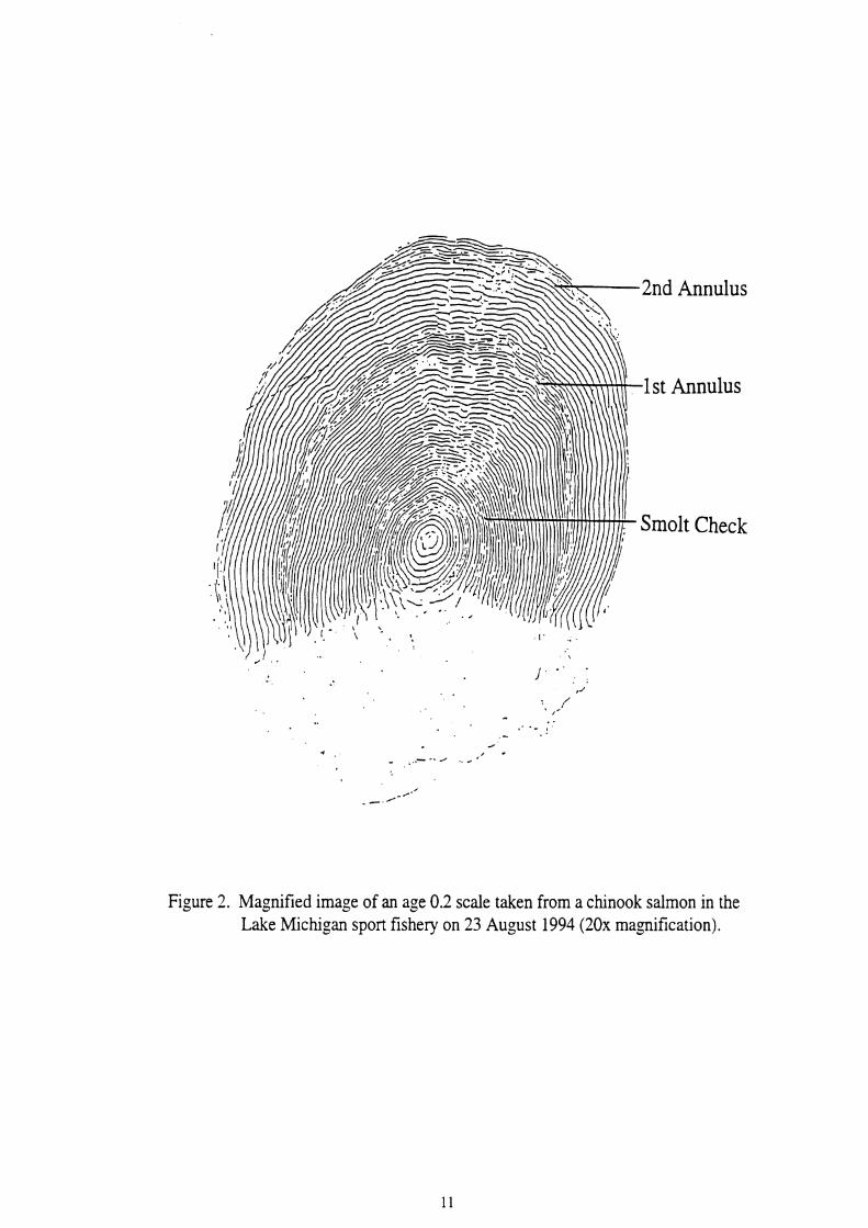
Figure 2. Magnified image of an age 0.2 scale taken from a chinook salmon in the Lake Michigan spon fishery on 23 August 1994 (20x magnification).

2nd
Che
rd Annulus
- 1 st Annulus
Figure 3. Magnified image of an age 0.3 scale taken from a chinook salmon in the Lake Michigan sport fishery on 10 July 1994 (lox magnification).

2nd Annuli
Annulus
st Annulus
Figure 4. Magnified image of an age 0.4 scale taken from a chinook salmon in the Lake Michigan sport fishery on 1 June 1994 ( lox magnification).

Focus
Figure 5 . Magnified image of an age 0.1 scale taken from a chinook salmon in the Lake Michigan sport fishery on 7 May 1994, with the first annulus just visible on the scale margin (20x magnification).

Recognition of scale erosion is also important in aging chinook salmon. Scale
erosion occurred in mature chinook salmon returning to the rivers to spawn. Eroded
scales were characterized by the presence of a jagged edge on the scale and the loss
of portions of the posterior margin of the scale (Figure 6 and 7). Scale erosion of
salmon is caused by the resorption of nutrients which are used for energy to migrate
upstream and for development of gonads (Wallin 1957). Resorption of the scale
could erode past one or more annuli, causing an underestimate in age. Scales
exhibiting erosion were not used in this analysis.
A pretrial was conducted to age chinook salmon which had CWT marks and
known ages. After this pretrial, it was determined that fish size could influence scale
age and bias estimates. Sizes of different age chinook salmon frequently overlapped,
adding to aging error. Scales were organized by time of harvest from spring to fall
and not by size class. Ordering by time of harvest allows the progession of annulus
formation to be observed and limits biases related to size.
Accuracy and precision estimates for scale ages -
Scale ages were compared to known ages to determine aging accuracy. The
percent of fish aged correctly was calculated for all ages separately and also combined
ages. The distribution of misaged chinook salmon was analyzed based on sex of fish
and maturity. A similar procedure was performed for vertebrae.
The precision or repeatability between scale readers was estimated using
statistical methods described by Bearnish and Fournier (1981) and Chang (1982).
Three scale readers (other than myself) independently aged the same sample of 76

Annulus
Figure 6. Magnified image of an age 0.2 scale taken from a chinook salmon in the Lake Michigan sport fishery on 27 August 1994, showing extensive erosion on the posterior margin (20x magnification).

Figure 7. Magnified image of a severely eroded chinook salmon scale from the fall river sport fishery, 20 September 1994 (15x magnification).

scales containing fish of ages 0.1 through age 0.3. The readers were aware of the
timing of annulus formation and were given time of harvest. Each reader used their
own prefered method of aging chinook scales; therefore, precision was estimated for
chinook salmon scales in general and not for my method of aging. These results were
used to calculate the average percent error (APE), coefficient of variation (V), and
index of precision (D). The average percent error was calculated using the number of
fish aged (N), the number of scale readers (R), the ith age of the jth fish (Xu) , and the
average age for the jth fish (Xi) using the equation:
V was calculated as the standard deviation divided by the mean for each fish, then was
averaged for all fish and represented as a percentage. D was obtained by dividing V
by the square root of R.
Results
A total of 302 chinook salmon were sampled from Lake Michigan between
May and September 1994 from my sport fishery sampling (152), U.S. Fish and
Wildlife Service sport fishery assessment (43), Ludington Pumped Storage assessment
gill nets (12), and Michigan DNR gillnets (95). Of the 302 samples, 206 were used
for scale analysis and 181 for vertebra analysis. Tag loss (fish exhibiting an adipose
fin clip with no CNT) and inability to collect certain data in the field reduced the total

samples collected to what could be used for each analysis. Fish exhibiting scale
erosion were also excluded from analysis.
Chinook salmon in Lake Michigan began to form an annulus on the outer
scale margin between mid-May and June, and 64.0 % of the sample had started
annulus formation by June (Table 1 and Figure 8). The annulus was completely
formed in 88.2 5% of the sample by the end of July. Age 0.1 and 0.2 chinook salmon
appeared to complete annulus formation earlier than age 0.3. Only 50.0 % of the age
0.3 fish exhibited a complete annulus formation by the end of July; however, the
sample size was two. There was also a decline in the percentage of fish with
complete annulus formation in August and September, with values of 85.7 % and
66.7 %, respectively.
Scale erosion was present in 14 of 83 fish collected between July and mid-
September (Table 2). All of these fish with eroded scales were mature and ranged
from age 0.2 to 0.4, and 7 1.4 % were males. Most of these fish (7 1.4%) were caught
in August. Some were harvested near river mouths by anglers, but all were taken
from Lake Michigan proper.
Accuracv and Precision
A total of 206 CWT chinook salmon was aged using scales. The overall
accuracy was 95.6 %, and all age classes appeared to be aged with equal accuracy
(Table 3). Aging 0.4 chinook salmon had 100 % accuracy; however, there was only a
sample size of two. Errors in aging never exceeded one year (Table 4). Misaged
chinook salmon were most commonly males (88% of the fish rnisaged)(Table 5);
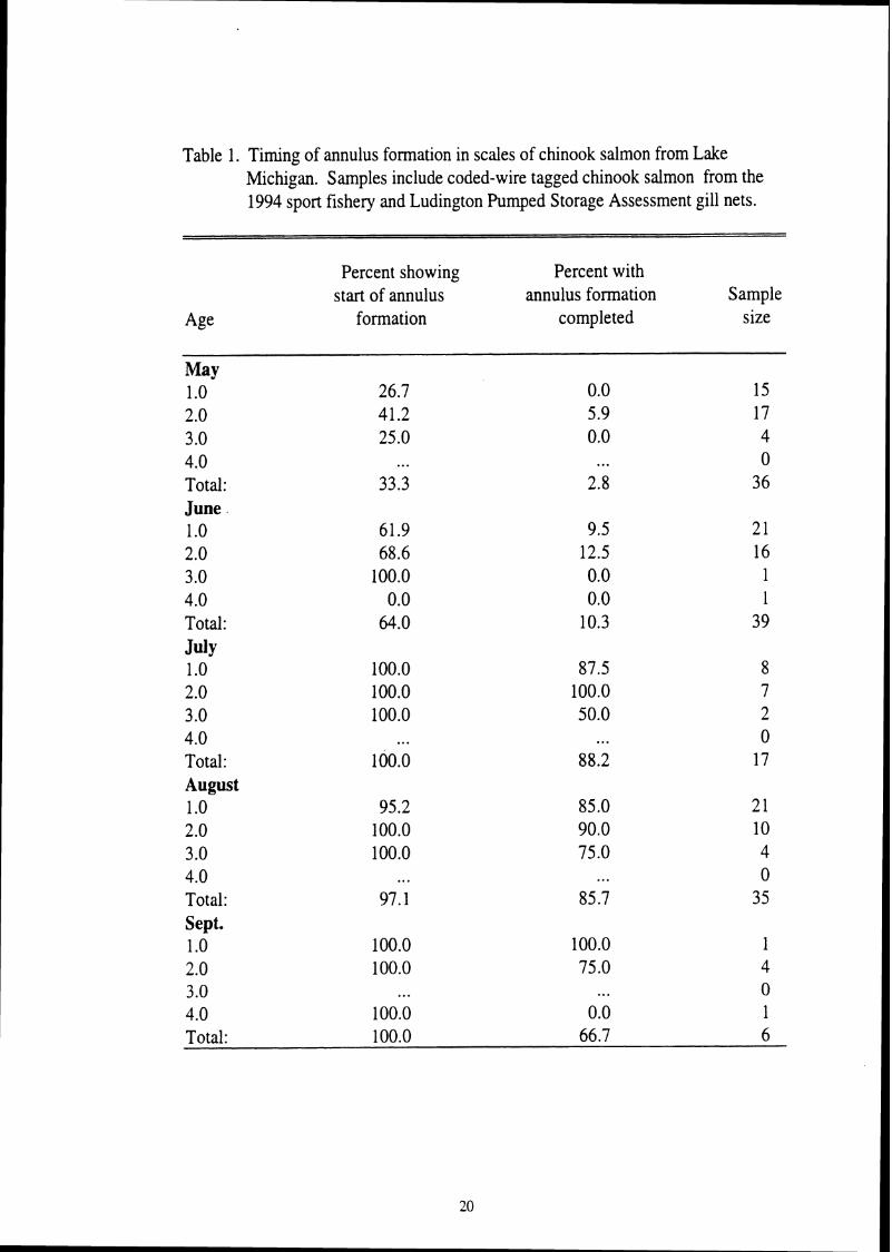
Table 1. Timing of annulus formation in scales of chinook salmon from Lake Michigan. Samples include coded-wire tagged chinook salmon from the 1994 sport fishery and Ludington Pumped Storage Assessment gill nets.
Percent showing Percent with start of annulus annulus formation Sample
Age formation completed size
May 1 .O 26.7 0.0 15 2.0 41.2 5.9 17 3.0 25.0 0.0 4 4.0 . . . . . . 0 Total: 33.3 2.8 36 June 1 .O 61.9 9.5 2 1 2.0 68.6 12.5 16 3.0 100.0 0.0 1 4.0 0.0 0.0 1 Total: 64.0 10.3 39 July 1 .O 100.0 87.5 8 2.0 100.0 100.0 7 3 .O 100.0 50.0 2 4.0 . . . ... 0 Total: 100.0 88.2 17 August 1 .O 95.2 85.0 2 1 2.0 100.0 90.0 10 3.0 100.0 75.0 4 4.0 ... . , . 0 Total: 97.1 85.7 35 Sept. 1 .o 100.0 100.0 1 2.0 100.0 75.0 4 3 .o . . . . . . 0 4.0 100.0 0.0 1 Total: 100.0 66.7 6

0 June - July August Sept.
Figure 8. Percent of chinook salmon having started and completed scale annulus formation by month for fish t aken from Lake Michigan in 1994.
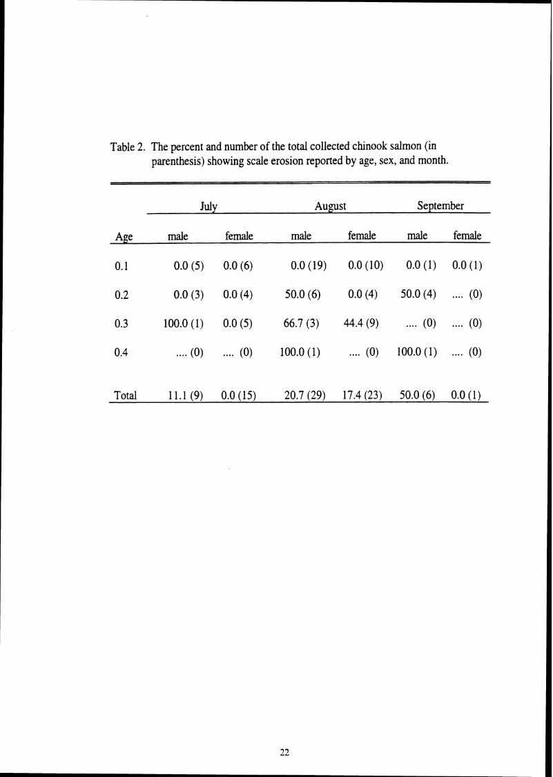
Table 2. The percent and number of the total collected chinook salmon (in parenthesis) showing scale erosion reported by age, sex, and month.
July August September
Age male female male female male female
0.1 0.0 (5) 0.0 (6) 0.0 (19) 0.0 (10) 0.0 (1) 0.0 (1)
0.2 0.0 (3) 0.0 (4) 50.0 (6) 0.0 (4) 50.0 (4) .... (0)
0.3 100.0 (1) 0.0 (5) 66.7 (3) 44.4 (9) .... (0) .... (0)
0.4 .... (0) .... (0) 100.0 (1) .... (0) 100.0(1) .... (0)
Total 11.1 (9) 0.0 (15) 20.7 (29) 17.4 (23) 50.0 (6) 0.0 (1)
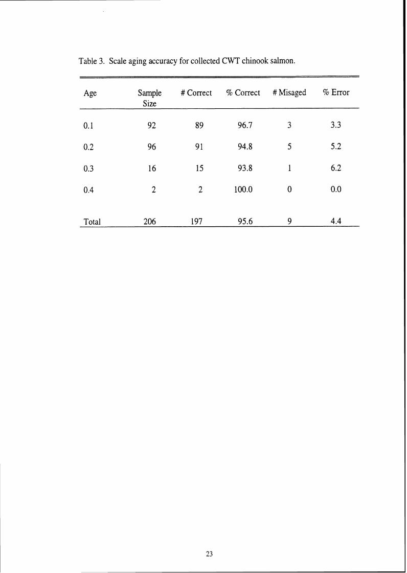
Table 3. Scale aging accuracy for collected CWT chinook salmon.
Age Sample # Correct 5% Correct # Misaged % Error Size
Total 206 197 95.6 9 4.4

Table 4. Differences between known age and age estimated by scales for CWT fish that were rnisaged.
Frequency CWT Scale Error Age Age Scale<CWT Scale>CWT in age (yr) 0.1 0.2 0 3 + 1 0.2 0.1 2 0 - 1 0.2 0.3 0 3 + I 0.3 0.2 1 0 - 1

Table .5. Distribution of the percent of misaged chinook salmon scales based on maturity and gender.
Mature Immature Total Male 44.4 (4) 44.4 (4) 88.8 (8) Female 11.1 (1) ..... (0) 11.1 (1)
Total 55.5 (5) 44.4 (4)

however, there was no significant difference in misaging frequency between sex and
maturity (p=0.342) based on Pearson's Chi-square statistic.
The accuracy of aging for all age classes of CWT chinook salmon using
vertebrae was 93.9 % with a sample size of 18 1 (Table 6). Age 0.1 chinook salmon
were the most accurately aged (loo%), while age 0.4 had the lowest accuracy of
aging (50%). Again, there was only a sample size of two for age 0.4 chinook salmon.
Differences between known and estimated ages never exceeded one year (Table 7).
Males were misaged more often than females, and more immature fish were misaged
than mature fish (Table 8). Most of these immature fish were small fish of the age 0.2
year class. There was no significant difference, however, between sex and maturity
(p=0.425, Pearson's Chi-square) based on misaged chinook salmon using vertebrae.
There were 10 discrepancies assigning age among the three scale readers in
the estimate of precision (Table 9). The index of APE calculated to be 3.63 %. The
V and D calculated to be 4.80 % and 2.77 %, respectively.
Discussion
Use of inaccurate ages may cause serious errors in fish population
management. Bearnish and McFarlane (1983) further list the significance of
validation for aging methods. I have demonstrated that scale and vertebrae aging can
be used accurately for age 0.1,0.2, and 0.3 chinook salmon from Lake Michigan. My
accuracy of aging vertebrae agrees with the results of Hesse (1994). However, the
ability to accurately determine age for age 0.4 chinook salmon still remains a question
using either scales or vertebrae. Due to the small sample size of known-aged fish, I

Table 6. Vertebra aging accuracy of collected CWT chinook salmon sampled.
Age Sample # Correct % Correct # Misaged % Error Size
Total 181 170 93.9 11 6.1

Table 7. Differences between known age and age estimated by vertebrae for CWT fish that were misaged.
Frequency CWT Vertebra Error Age Age Vert<CWT Vert>CWT in age (yr) 0.2 0.1 7 0 - 1

Table 8. Distribution of the percent of rnisaged chinook salmon vertebrae based on maturity and gender.
Mature Immature Total Male 9.1 (1) 63.677) 72.7 (8) Female 9.1 (1) 18.2 (2) 27.3 (3)
Total 18.2 (2) 81.8 (9) mostly small sized 0.2 year olds

Table 9. Estimated scale ages and associated APE, V, and D of 3 readers who each analyzed scales from 76 chinook salmon taken in Lake Michigan.
Estimated Age Known Reader Reader Reader
n Age 1 2 3 APE V D
2 1 1 1 1 1 0 0 0

could not determine accuracy of age 0.4 fish with confidence. Age 0.4 chinook
salmon probably represent a small percentage of the total population in Lake
Michigan based on angler harvest, but the large size of age 0.4 chinook salmon is
important to the fishery (Rakoczy and Svoboda 1994).
Scale aging of chinook salmon is more accurate for fish taken from Lake
Michigan than from the Pacific Ocean. Godfrey et al. (1968) found that scales were
only 75 % accurate using chinook salmon from Columbia hver . This decreased
accuracy can be accounted for by the more complex life history of chinook salmon in
Columbia River and the lack of information used by the scale readers. Godfrey et al.
(1968) states that chinook salmon may spend several years in the river before
migrating to the ocean and may not return to rivers for up to six years. This life
history is much more variable than for chinook salmon in Lake Michigan. The scale
readers in that study also knew only that chinook salmon scales were being read, not
any information related to annulus formation dates.
Knowledge of the timing of annulus formation, recognition of scale erosion,
awareness of smolt checks, and the use of information such as date of harvest can
help increase scale aging accuracy. The timing of the annulus formation is important
when aging fish harvested in spring, as the last annulus may not be formed until late
May to July. Scales exhibiting erosion should not be aged with confidence due to the
potential loss of annuli causing underestimation of age. For these reasons, harvest
date is important information to know about an individual fish. Harvest date indicates
whether a formed annulus will be present at the scale margin. In initial aging, it is
also beneficial to order a sample by date collected from spring to fall so that the
progression of annulus formation can be followed. Ordering by date also reduces
potential biases associated with ordering scale samples by size of fish. For example,
lengths of age 0.0 chinook salmon in the fall overlap with age 0.1 chinook salmon in
the spring. If date of harvest is not considered, age 0.1 fish in the spring can easily be
confused with age 0.0 fish in the fall because neither show an annulus formation.
Most error in aging chinook salmon from Lake Michigan using scales
occurred on males and with fish age 0.2, which may be due to varying growth in these
groups causing unusual scale characteristics. Fast growing fish are typically easier to
age because there are wide areas in the scale between annuli. If this fast growth
occurs in the spring, recognition of an annulus may become more difficult due to
fewer circuIi being closely grouped. In these cases, it is also important to find
crossing over of the circuli.
Aging with vertebrae was also accurate, with overall accuracy (93.9%) being
slightly lower than scale accuracy (95.6%). Vertebral aging accuracy was also
slightly lower in this study than the estimate of 95.4% made by Hesse (1994) using
lake harvested chinook salmon. Like scale aging error, most vertebrae aging error
was with males. However, more vertebrae from immature chinook salmon were
misaged compared to mature fish. Most of these errors were small sized fish of the
age 0.2 year class. These small age 0.2 vertebrae may not have strong areas with
opaque and translucent zones (Hesse 1994), or zones representing the first annulus
might be confused with smolt checks. Although the same techniques were applied,

different scopes and lab conditions were used by Hesse (1994) which may influence
accuracy results. The low sample size of age 0.4 chinook vertebrae makes the aging
accuracy using vertebrae of age 0.4 fish still in question.
Scale aging of chinook salmon from Lake Michigan also appears to be precise
based on comparative results of three readers. The resulting 3.63 % APE and 4.80 %
V are relatively low, and low values of APE and Vindicate high precision or
repeatability between readers (Beamish and Fournier 198 1, Chang 1982). The D
value shows that an average of 2.77 % of the total error was contributed by each
observation of age (Chang 1982).
Precision of scale aging and vertebrae aging are equal based on three readers.
There was no significant difference between my scale aging and vertebrae aging
precision estimates made by Hesse (1994) based on APE, V, and D (p>0.05, t-tests).
Differences in age assignment rarely deviated from one year with chinook salmon. If
errors frequently departed one or two years in age, this would indicate poor precision
because chinook salmon only live up to five years in Lake Michigan.
The following set protocol for aging chinook salmon from Lake Michigan
incorporates life history complexity and its effect on aging: 1) An annulus consists of
a close grouping of circuli with evidence of crossing over of the circuli. 2) A smolt
check is a close grouping of circuli about 7 to 14 circuli counts from the focus. 3) A
stream annulus is a close grouping of circuli with evidence of crossing over of the
circuli after a tight band of 14 to 2 1 circuli from the focus followed by a smolt check
(Carl 1980). 4) Annulus formation occurs between May and July. 5) Scales

exhibiting erosion should be eliminated from analysis. 6) Vertebrae should be used
as an alternative to scales for mature fish harvested in Lake Michigan and at blocking
harvest weirs in the fall.
There are many advantages to using scales for aging fish. Two main
advantages are the ease of sampling and handling, as well as the ability to return fish
alive once scales have been removed. In addition estimates of growth can easily be
made from scales using back calculation. Finally, there are historical collections of
scales which can be reanalyzed. The main disadvantage of scales in aging chinook
salmon is that scale erosion occurs in the fall. Most mature chinook salmon harvested
after August exhibited scale erosion, and this is a large disadvantage because chinook
become more vulnerable to angling in the fall as they stage to migrate. Weir
harvested scales are also very difficult to age because of scale erosion.
Hesse (1994) explained the advantages and disadvantages of aging with
vertebrae. The most important advantage of using vertebrae is that erosion or
distortion does not occur to vertebrae. Vertebrae can be used to age mature chinook
salmon harvested in the fall sport fishery and at weirs.
Based on the young age and fast growth of chinook salmon in Lake Michigan,
it is expected that aging of their bony structures would be accurate and precise. Lake
trout, which are slow growing and live as long as 20 years (Becker 1983), are more
difficult to age. Growth declines with age malung annuli difficult to identify in bony
structures such as scales in lake trout (Johnson 1976, Sharp and Bernard 1988).
However, aging of chinook salmon becomes more difficult with a complex life

history. Most temperate fishes form an annulus once a year during slow growth in
winter (Tesch 1968). Chinook salmon also exhibited smolt checks in bony structures,
which are produced during slow growth periods while migrating downstream. Annuli
in chinook salmon usually occur after the smolt check but may occur before in stream
yearlings (Carl 1980, Seelbach and Beyerle 1984). Within Lake Michigan, chinook
salmon show variation in growth and age at maturity and mature fish returning to
natal streams using resorb energy stored in body parts including scales. This
complexity in the life history of chinook salmon along with the late annulus formation
can make aging difficult. The suggested aging protocol with scales and vertebrae
should decrease this difficulty and is a valid technique.

CHAPTER THREE
Growth Rate by Age, Sex, and Maturity Classes of Chinook
Salmon in Lake Michigan
Introduction
Knowledge of fish growth can be useful in assessing the health of individuals
and populations of fish. Understanding the factors that influence growth are also
important in comparing different populations of the same species. These factors,
which include abiotic factors (such as temperature, oxygen, salinity, and light) and
biotic factors (such as ration, fish density, competition, predation, food abundance,
and food availability) are reviewed in Tesch (1968), Weatherley and Gill (1987), and
Diana (1995). Because of these factors, growth can vary with season and life history
characteristics such as maturity, sex, and age (Weatherley and Gill 1987).
Pacific salmon can have very complicated life histories (Chapter Two).
Healey (1991) summarized life history observations of chinook salmon from the
Pacific Ocean. Male chinook salmon tend to have more rapid growth and mature
earlier than females. Based on MDNR weir data, male chinook salmon in Lake
Michigan also grow faster and mature earlier than females (Hay 1992, Pecor 1992).
However, there is little data on age-specific growth of chinook salmon, as well as
growth differences based on gender or maturity. Chapter Two evaluated an accurate
aging system, including validation with CWT fish, to use on fish at large in Lake
Michigan. This allows an accurate evaluation of growth differences among different
age classes, gender, and maturity. Growth rates can be determined with confidence
because there will be no age misclassification; therefore, the differences in growth can
be associated with the particular life history characteristics. One main purpose of this
chapter is to investigate current growth rates in chinook salmon at large in Lake
Michigan.
The methods for analyzing growth are many. These methods can be grouped
into the following categories: 1) static analysis or the comparison of mean size of
each cohort once in a year; 2) cohort analysis or determining mean size of each cohort
several times during the year; 3) individual analysis which involves measuring the
change in size of marked individuals; and 4) back calculation which uses bony parts
to calculate growth hstory (Bagenal and Tesch 1978, Casselman 1987, Diana 1995).
The method of back calculation will be emphasized in this and the following Chapter.
Back calculation is a technique of inferring a fish's length using a set of
measurements made on bony structures. Tesch (1968), Weatherley and Gill (1987),
and Francis (1990) give thorough reviews of the historic and current methods used in
back calculation as well as the types of calcified structures measured. The use of
back calculation can increase the amount of length-at-age data (Shafi and Jasim 1982)
and allows estimation of lengths at ages rarely observed for some species (Francis
1990). Growth rates obtained from back calculated lengths have also been used to
compare cohorts (Frost and Kipling 1980) and to relate growth due to various
physical and biological factors (Weatherley and Gill 1987). Most back calculation
methods use a relationship between the body length and scale radius of the fish. This
can be a linear or curved relationship (Tesch 1968, Weatherley and Gill 1987, Francis

1990). The Fraser-Lee method (Hile 1970, Carlander 198 1, Frie 1982) requires a
linear relationship and uses this line to calculate the intercept which is described as the
length of the fish at scale formation. The method uses the proportion of body length
to scale length for each fish to back calculate individual length, which is an advantage
because it allows variation between individuals unlike regression methods (Carlander
198 1). Carlander (1949) cautions that variation in scales can lead to error in body-
scale relationships. A comparison of lengths at capture avoids errors due to body-
scale relationship but creates problems due to differences in time of capture. Another
common problem with back calculation is Lee's Phenomenon, which occurs when
computed lengths at a given age are smaller than observed lengths. Lee's
phenomenon is more pronounced when calculating lengths of young fish from much
older fish (Tesch 1968). These problems can be avoided by calculating lengths only
to the last annulus which offers a more valid method for comparative purposed
(Carlander 1 949).
The second purpose of this chapter is to compare growth rates between sport
harvested and gill net harvested chinook salmon in Lake Michigan. It is common to
group these two sampling methods to increase sample size. With decreased
abundance and catches of age 0.3 and age 0.4 chinook salmon, it may be necessary to
combine different harvesting methods to increase sample size. However, these
methods of harvesting may select different size chinook salmon which could bias
growth analyses. For example, Miranda et al. (1987) found anglers caught longer
largemouth bass Micropterus salmoides than did electrofishing or cove rotenone

sampling. Anglers appear to catch the largest fish of each cohort. They may also
catch the most aggressive fish, which may have faster growth rates than a typical fish
from that population (Quinn and Unwin 1993). Therefore, before the two collections
can be combined, it is important to compare the two collecting methods for sampling
bias.
The main objective of this chapter is to compare current growth of chinook
salmon from Lake Michigan between fish with different life history characteristics
such as age, sex, and maturation state. The second objective is to compare lengths of
chinook salmon from two different sampling gears, angler and gill net harvests. Both
objectives involved back calculation using scales.
Methods
Sample Source and Preparation
Coded-wire tagged (CWT) chinook salmon as described in Chapter Two were
sampled from the eastern Lake Michigan sport fishery and MDNR R. V. Steelhead gill
nets between May and September 1994. Sport fishery and gill net samples were
combined from each port to create one sport fishery sample and one gill net sample
for the entire year. Gill net samples came from the eastern shoreline of Lake
Michigan from New Buffalo in the south to Little Traverse Bay in the north (Figure
9). Chinook salmon were targeted during spring in the south (May), summer in
central (June),and fall in the north (July-August) region of Lake Michigan. Gill nets
consisted of 9-m deep monofilament twine with mesh sizes of 9 cm to 16.5 cm with a
2.5 cm interval (Rybicki 1995).

MICHIGAN
Grand Haven
1 cm - 0 24.1km
Scale of km
Figure 9. A map of Lake Michigan and location of sampled ports.
The sport fishery was sampled from Saugatuck in the south to Leland in the
north (Figure 9). Port selection was dependent on chinook salmon catch; therefore,
ports were frequently sampled if catch rates of chinook salmon were high compared
to the rest of eastern Lake Michigan. Targeted areas at each port included cleaning
stations where angler concentrations were high. Data were collected by myself or by
trained, volunteers from all observed CWT fish.
Weight (to 1 g), total length (to 1 mm), sex, gonad development, scales (taken
between the dorsal and adipose fins above the lateral line), visual checks for BKD
(swelling andlor pustules in the kidney) and noses (cut just behind the eye) containing
tags were collected. Immature gonads were described as small, colorless, and found
close to the vertebral column, while mature gonads were enlarged, colorful (orange
for ovaries and white for testes), and filled the body cavity. Known fish ages from
CWTs were provided by MDNR. Scales were pressed in acetate film.
Growth Analysis
Back calculation of mean total length at age using scales was used to compare
growth of sport and gill net harvested chinook salmon. Lengths were back calculated
only to the last annulus not to previous annuli; therefore, the mean length of age 0.1
fish is the back calculated length to the 1 st annulus of fish harvested at age 0.1 only.
Similarly, mean length of age 0.2 is back calculated length to the 2nd annulus of fish
harvested at age 0.2. Back calculating lengths to the last annulus avoids problems
associated with Lee's phenomenon. The Faser-Lee method of back calculation was
used (Hile 1970, Carlander 198 1, Carlander 1982, and Frie 1982). This method

required computation of the simple linear regression of fish length versus scale radius
( I ) used in the back calculation formula (2) to estimate total lengths as follows:
( I ) L = a + b ( ~ , )
Where S, is the scale measurement to the edge of the scale, LC is the length of fish at
capture, a is the intercept of the body-scale regression in equation (I), Si is the scale
measurement to the ith annulus, and Li is the length of fish at the ith annulus.
An annulus was defined as close grouping of circuli with crossing over of the
circuli (see Chapter Two and Figures 1-5). Measurements to each annuli and to the
edge of the scale were made with a microcomputer Java projecting system (3x
magnification) (Acker and Mitchell 1988). These measurements from the focus to the
edge of the scale were made through the longest radius which was approximately 20"
from the perpendicular axis of the scale (see Figure 10).
Separate regressions between total length and scale radii were calculated for
fish harvested by sport or gill nets to estimate a in equation (1) which was then used
in equation (2). Predicted total lengths from equation (2) were compared between
chinook salmon harvested by sport and gill net. The mean back calculated total
lengths of the two collecting methods were tested for equivalence using t-tests.
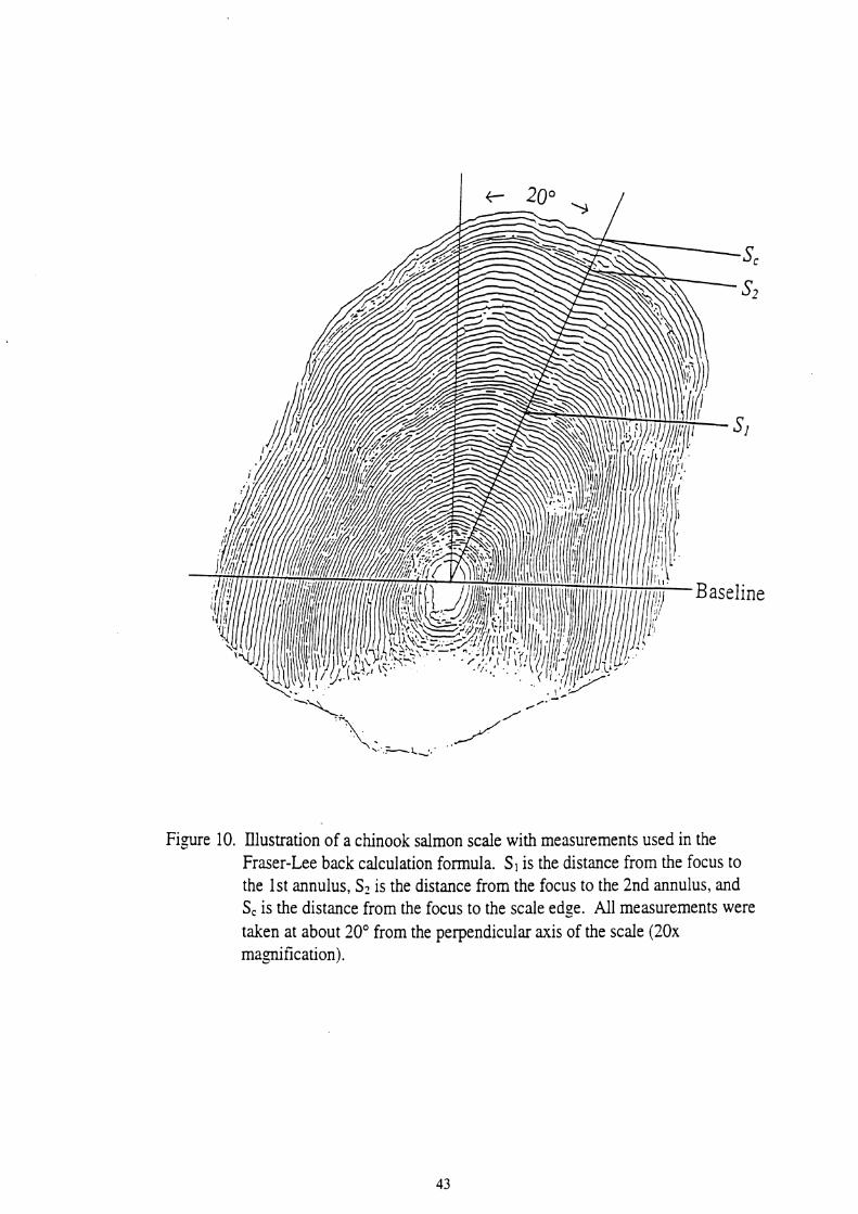
Figure 10. Illustration of a chinook salmon scale with measurements used in the Fraser-Lee back calculation formula. S, is the distance from the focus to the 1st annulus, S2 is the distance from the focus to the 2nd annulus, and S, is the distance from the focus to the scale edge. All measurements were taken at about 20" from the perpendicular axis of the scale (20x magnification).

Comparisons with t-tests were also made by age and gender. Assumptions of
normality and equal variances were tested using coefficients of skewness, kurtosis,
and F-tests for equal variance. All tests were run at the 5 9% level of significance
using SPSS (Norusis 1993).
Results
Scales and size data from a total of 130 sport and 75 netted fish were used to
back calculate growth. Fish lengths and scale radii were plotted and regressed for
sport harvested (Figure 11) and gill netted (Figure 12) chinook salmon. The
equations in Figures 11 and 12 both had good linear relationships yielding R' values of
0.92 and 0.83, respectively.
The mean back calculation results (Table 10) based on age and gender met
assumptions of normality and homogeneity. There were no significant differences in
mean length between sport caught and gill netted chinook salmon for age 0.1 males,
age 0.1 females, and age 0.3 females. There was a significant difference in mean
length at age 0.2 for males and age 0.2 females between the two methods of harvest,
with length being larger in gill netted fish. There were more mature age 0.2 males in
the gill net harvest (n=l l ) than in the sport harvest (n=5).
There were no significant differences between mature or immature age 0.2
chinook salmon with the two sampling methods (Table 11). Immature males taken by
a collection gear were significantly smaller than mature males. Mean length for
immature age 0.2 females was also significantly lower than mature females for gill net

0 0.5 1 1.5 2 2.5 3 3.5 4 4.5
Scale Radius (mm)
Figure 1 1. Plot of scale radius and fish total length for chinook salmon harvested by sport in Lake Michigan, 1994.

0 0.5 1 1.5 2 2.5 3 3.5 4 4.5
Scale Radius (mm)
Figure 12. Plot of scale radius and fish total length for chinook salmon harvested by gill net in Lake M i ch i ,~ , 1994.
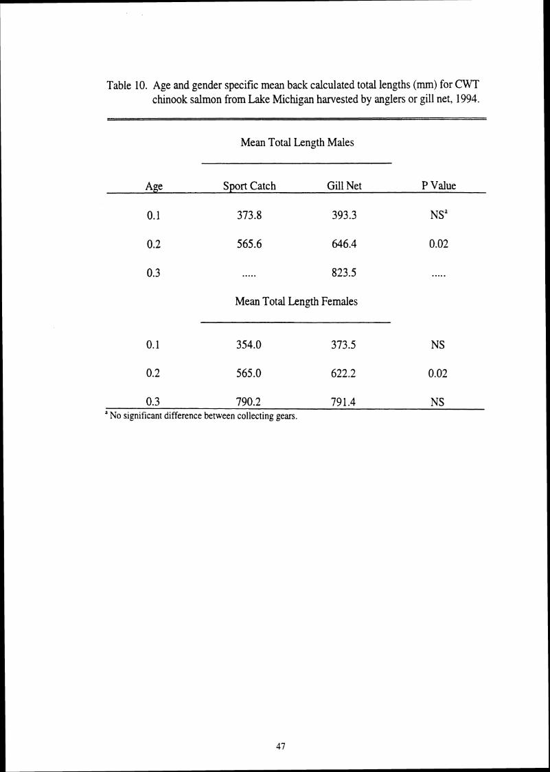
Table 10. Age and gender specific mean back calculated total lengths (mrn) for CWT chinook salmon from Lake Michigan harvested by anglers or gill net, 1994.
--
Mean Total Length Males
-
Age Sport Catch Gill Net P Value
0.1 373.8 393.3 NS"
0.2 565.6 646.4 0.02
0.3 ..... 823.5 .....
Mean Total Length Females
0.3 790.2 791.4 NS a No significant difference between collecting gears.

Table 1 1. Age 0.2 gender and maturity specific mean back calculated total lengths (mrn) for sport and gill net harvested chinook salmon from Lake Michigan, 1994.
Age 0.2 Males
Sport Catch Gill Net P Value
Immature 530.9 570.0 NS"
Mature 690.4~ 688.1' NS
Age 0.2 Females
Immature 565.0 581.5 NS
Mature .... 687.4d ....
a no significant difference between collecting gears. significant difference between sport caught mature and immature males (p=0.001). significant difference between gill netted mature and immature males (p=0.01). significant difference between gill netted mature and immature females (pc0.001).

harvested chinook. The sample size was too small for age 0.2 females to test sport
caught females by maturity status.
Since the significant difference between harvest gears at age 0.2 in Table 10 is
due to maturity composition of samples and not due to other harvest gear biases, the
two samples were combined (Table 12). Again, immature males and females were
significantly smaller in length than mature males and females.
Lengths were also back calculated to earlier ages (Table 13) to look at
different growth trajectories based on life history traits. Yearly growth increments
were plotted for females (Figure 13) and males (Figure 14). Mature males and
females were larger in total length and had slightly higher slopes indicating better
growth rates.
Discussion
Maturity is size related for chinook salmon in Lake Mchigan since the largest
members of the younger age classes matured (Figures 13 and 14). Males also seemed
to mature at a younger age than females; however, there was no significant difference
in total length between males and females. The maturity results agree with MDNR
weir data (Hay 1992, Pecor 1992) and also with Healey's (1986) suggestion that male
chinook salmon show more variation in size at maturity than females from Pacific
populations. Berg (1978) also found no significant differences in age specific growth
between sexes in chinook salmon from Lake Superior.
In general, age at maturity is inversely related to growth in salmon (Neilson
and Geen 1986, Heath et al. 1991, Bohlin et al. 1994, Mange1 1994), charr (Matuszek
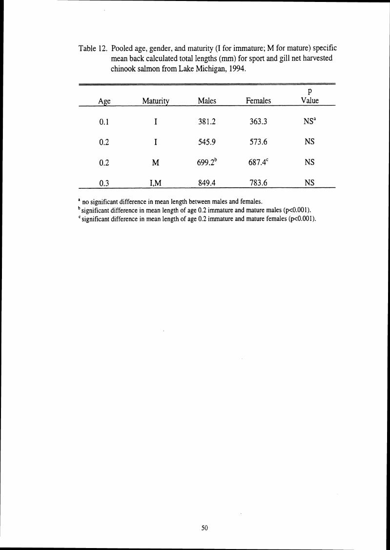
Table 12. Pooled age, gender, and maturity (I for immature; M for mature) specific mean back calculated total lengths (rnm) for sport and gill net harvested chinook salmon from Lake Michigan, 1994.
P Age Maturity Males Females Value
0.1 I 38 1.2 363.3 NS"
a no significant difference in mean length between males and females. significant difference in mean length of age 0.2 immature and mature males (p<0.001). significant difference in mean length of age 0.2 immature and mature females (p<0.001).
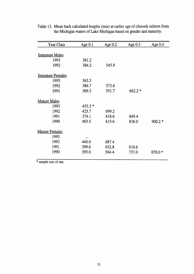
Table 13. Mean back calculated lengths (mm) at earlier age of chinook salmon from the Michigan waters of Lake Michigan based on gender and maturity.
Year Class Age 0.1 Age 0.2 Age 0.3 Age 0.4
Immature Males 1993 381.2 1992 384.2 545.9
Immature Females 1993 363.3 1992 386.7 573.6 1991 369.3 55 1.7 662.2 *
Mature Males 1993 453.3 * 1992 425.7 699.2 1991 374.1 618.6 849.4 1990 403.5 615.6 836.0 900.2 *
Mature Females 1993 ... 1992 440.0 687.4 1991 399.6 632.8 8 10.6 1990 395.0 564.4 737.0 870.0 *
* sample size of one.

Females
Figure 13. Lake Michigan chinook salmon back calculated annual growth increments for females based on total lengths of pooled sport and gill net harvested fish, 1994.
-
-
-
-
-
-
-
-+ Age 0.2 Immature
-0- Age 0.2 Mature
--+- Age 0.3 Mature
-
I I

Males
Figure 14. Lake Michigan chinook salmon back calculated annual growth increments for males based on total lengths of pooled sport and gill net harvested fish, 1994.
-
-
-
-
-
-
-
4- Age 0.2 Immature
+ Age 0.2 Mature
-+ Age 0.3 Mature
-
1 . I

et al. 1990, Trippel 1993) and other fishes (Pitt 1975, Hay et al. 1988, Hartman and
Margraf 1992, Houthuijzen et al. 1993). Jobling and Baarduik (1 99 1) and Jobling et
al. (1993) found that mature males grew faster than immature male and female Arctic
charr Salvelinus alpinus. Sexual dimorphism in size is common in some fishes
(Casselman 1987). Male steelhead trout 0. mykiss grow faster than females in
saltwater (Parker and Larkin 1959). Most of the difference in size between sexes in
salmonids seems to be based on maturity, where faster growing fish mature earlier. In
my analysis, I compared chinook salmon based on sex and maturity and found no
differences in size between sexes. Parker and Larkin (1959) may have had different
results if they had analyzed growth based on sex and maturity rather than just sex.
Factors other than growth may also influence age at maturity. Quinn and
Unwin (1993) indicate that selection (artificial or natural) against older fish could be a
mechanism regulating age at maturity. With the presence of BKD in Lake Michigan,
I believe that there is a selection against older fish which could reduce the age at
maturity. In Atlantic salmon, Riddell (1986) found that the fishery reduced age at
maturity by genetically selecting against older fish. With a large heritable component
in age at maturity for chinook salmon (Hard et al. 1985), hatchery practices could
also have an effect on size and age at maturity in Lake Michigan. It is not evident
that age at maturity has changed due to size selection from BKD or hatchery
practices.
With low population levels of age 0.3 and 0.4 chinook salmon in Lake
Michigan, the combination of age and growth data from sport and gill net harvested

fish may be important to increase sample sizes. My data suggest that there are no
differences between the two methods based on age, gender, and maturity specific
mean total lengths. Anglers seem to catch the same size fish as gill nets, contrary to
the findings of Miranda et al. (1987) with largemouth bass. A larger sample size of
age 0.3 and 0.4 chinook salmon would increase confidence in these results. These
data support the use of pooling sport caught and gill netted chinook salmon for
growth analyses. However, it would be inappropriate to pool angler and gill net
harvested chinook salmon unless samples are stratified by maturity, gender, and age.
There were, however, slight differences in the slopes and intercepts (a) of
length to scale radii relationships between the sport and gill netted harvested fish.
Carlander (1982) suggested that most variation in a is not due to population
differences but is due to measuring scales at different angles, collecting scales from
different areas of the body, season of collection, and samples with poor representation
of small sizes. The angles of measurement and the season of collection were the same
for both data sets in this study. There may be differences in scale sampling areas on
the body between the two data sets. I collected the sport caught scales and MDNR
employees collected the gill netted scales. There was also a lack of fish under 25.4
cm (10.0 in.) since this is the legal size limit for angled chinook salmon in Lake
Michigan, and since mesh sizes for gill nets were too large to catch a representative
sample of small fish.
Some reverse Lee's phenomenon appeared to be occurring with back
calculated lengths from the pooled data in Table 13; age 0.1 lengths back calculated
from older aged (age 0.2'0.3, or 0.4) chinook salmon are larger than back calculated
lengths of chinook salmon harvested at age 0.1. Tesch (1968) gave a good
description and literature review of Lee's phenomenon. Reverse Lee's phenomenon
occurs when back calculated lengths at a given age are larger than observed lengths at
that age. Neilson and Geen (1986) also found reverse Lee's phenomenon when back
calculating lengths of chinook salmon using otoliths. Some causes of reverse Lee's
phenomenon could be selective natural mortality (greater survival of larger fish),
selective fishing mortality, or non random sampling of the population (sampling the
larger representatives). Some of these causes could occur in Lake Michigan. Larger
chinook could be more vulnerable to the sport fishery; however, I found no difference
in size between angler and gill net harvested chinook salmon in Lake Michigan. BKD
may be selecting against slow growing or small fish, increasing the number of larger
fish surviving to an older age. The low numbers of age 0.4 chinook salmon in the
present Lake Michigan population could be due to low survival of small fish due to
BKD.
The differences in growth of chinook salmon based on gender and maturity
will be important to consider in future studies involving growth. Predator prey
models developed for salmonids from Lake Michigan could be improved by
considering these different growth trajectories. It will also be useful to management
to monitor ages at maturity to see if changes occur with size selection from BKD and
current hatchery practices. Evidence from the reverse Lee's phenomenon suggests
that smaller hence slower growing fish are more vulnerable to BKD than faster

growing fish. The critical period may be associated with the growth achieved by the
first year of life; therefore, more research is needed to examine the early life history of
chino0.k salmon in Lake Michigan. This research may reveal limiting factors on the
growth of juvenile and yearling fish.
CHAPTER FOUR
Comparison of Size at Age for Chinook Salmon in Lake Michigan, 1983-1993
Introduction
A quantitative comparison of historical and current growth of chinook salmon
may give some insights to their recent decline in Lake Michigan (Chapter One). A
decrease in growth could be associated with declining alewife numbers, and it may
indicate stress due to forage decline as the mechanism causing the outbreak of BKD.
If there was no change in growth, perhaps another hypotheses for the outbreak of
BKD would be more logical. Estimation of historic growth rates would also be
beneficial to calibrate existing and future predator prey models for Lake Michigan
salmonids (Stewart et al. 1981, Stewart and Ibarra 1991).
The ability to accurately age lake harvested chinook salmon using scales
allows the estimation of age specific growth with confidence. Historic size data and
scales can be analyzed to determine size at age using back calculation methods
described in Chapter Three. The longest data set including scales from lake harvested
fish is from the MDNR creel survey for Lake Michigan which began in 1983
(Rakoczy and Svoboda 1994). MDNR weir data are also available, but scales can not
be aged accurately because of erosion which may lead to error in growth rates.
Vertebrae have not been collected as weir data, even though vertebrae are the best
calcified structures to use for aging mature chinook salmon (Hesse 1994).
The objectives of this chapter are to determine historic age and growth of
chinook salmon by back calculation and compare past and present growth rates in

Lake Michigan. Another objective is to compare growth based on location of
harvest. Traditionally, the sport fishery for chinook salmon in Lake Michigan begins
in early spring in the southern part of the lake, and as the year progresses, the fishery
moves north (Rakoczy and Svoboda 1994). Assuming that this movement in the
fishery represents a seasonal movement in fish, then a large number of chinook
salmon overwinter or at least spend early spring in the southern part of the lake. A
growth comparison for chinook salmon harvested in the spring may give some
understanding to why this migration occurs. If the migration of chinook salmon is
following a migration of forage fishes, then spring harvested chinook salmon should
show better growth in the south than in the north. Warmer water temperatures in the
south may also improve chinook salmon growth.
Met hods
Biological data were taken from samples collected by MDNR creel clerks
between New Buffalo and Charlevoix. Clerks sampled anglers from the Michigan
waters of Lake Michigan during open water season between 1 April and
3 1 March using stratified random sampling (Rakoczy 1992). Biological were taken
on a percentage of fish sampled in the field at each port. These data consisted of total
length (to 1 rnrn), weight (to 1 g), and scales. On occasion, observations of sex and
maturity were also recorded. Creel clerks were trained each year to take scales from
between the dorsal and adipose fin and above the lateral line.
Scales were pressed and aged using techniques described in Chapter Two.
Scales exhibiting erosion were not used for analyses. An average of three
measurements on scales from each fish were made on a Java Projection Computer
System (Acker and Mitchell 1988) to determine back calculated lengths using the
Fraser-Lee Method (see Chapter Three for details). Scale increments and fish lengths
were input in the DISBCAL computer package (Frie 1982) for back calculation. A
common intercept of 86 mm was used for all years (Carlander 1982, Chapter Three).
Samples from each port were combined into one Lake Michigan sample for
each year to compare growth. Mean back calculated lengths at each age were
compared for each year. Lengths were calculated back to the time of annulus
formation, which occurs between June and July, for that current year and age of fish
only. For example, mean length of age 0.2 fish in 1983 represents total lengths back
calculated to the 2nd annulus of age 0.2 fish harvested in 1983; it was not back
calculated total length to the 2nd annulus of age 0.3 or 0.4 fish harvested in 1984 or
1985. Only age 0.1 through 0.4 chinook salmon were analyzed. Age 0.5 fish and
any chinook salmon that appeared to have one year of stream residency were not used
because those life history types have not been validated using scale methods.
Length of an individual fish rarely decreases with time; however, weight may
increase or decrease for any given length of an individual fish (Wootton 1990). These
changes in weight may indicate more subtle changes in growth relative to length.
Therefore, the Fulton Index of condition was also compared because condition is
more sensitive to subtle changes in growth. The Fulton Index was recommended for
fish showing isometric growth (w=~L)) where weight is symmetric with length by a
factor of three (Tesch 1968, Anderson and Gutreuter 1983). Chinook salmon from
Lake Michigan have this isometric growth with a slope of 3.08 based on data from
1983 to 1993 (see Table 17). The Fulton Index (FI) of condition was calculated
using the following equation (Anderson and Gutreuter 1983):
where W is weight (g), L is length (rnrn), and X (100,000) is an arbitrary scaling
constant. Back calculated length of each individual fish was used to compute
individual weight. Weights were then estimated from weight-length relationships
calculated from fish harvested before 30 June for each year. Therefore, lengths,
weights, and condition were based on spring measurements.
Mean back calculated lengths and Fulton Indices were also used to compare
growth between chinook harvested in the north and south sections of Lake Michigan
before 30 June. Chinook harvested from Muskegon and to the south were pooled to
form the south section, while the north section consisted of all ports from Ludington
north. 'To increase sample size, 1985 and 1986 samples were combined. These years
were before the onset of BKD.
Total length was back calculated only to spring for each age of fish;
henceforth, this variable will be called back calculated length. Back calculated lengths
and Fulton Indices were compared for fish sampled from 1983 through 1993.
Assumptions of normality and equal variances were tested using coefficients of
skewness, kurtosis, and F-tests for equal variance (Norusis 1993). Age 0.1 and 0.2

chinook salmon had unequal variances in mean back calculated lengths, so
nonparametric Kruskal-Wallis and Mann-Whitney U tests were used to determine
differences among and between years. Mean back calculated lengths of age 0.3 and
0.4 fish were compared with ANOVA'S, and multiple comparisons were made using
Bonferroni's test. All ages had unequal variances with Fulton Index data so Kruskal-
Wallis and Mann-Whitney U tests for equal means were used. With the comparison of
back calculated lengths and Fulton Indices for fish from the north and south, F-tests
for equality of means were used for normally distributed data with equal variances and
Kruskal-Wallis and Mann-Whitney U tests of equal means were used otherwise. All
tests were performed at the 5 % level of significance using SPSS (Norusis 1993).
Results
Most chinook salmon in the sample were harvested from Grand Haven south
and from Manistee north. A total of 2,647 scales were aged and measured for
samples from 1983 through 1993. The proportion of the samples comprising each
age class decreased for ages 0.3 and 0.4 fish and increased for age 0.1 fish from 1983
to 1993 (Table 14). The average age of salmon in the sample also decreased from a
high of 2.59 years in 1986 to 1.53 in 1993. The number of chinook exhibiting stream
annuli was variable among years and comprised a low percent of total catch (Table
15). Age 0.5 chinook salmon were only observed in 1987 with a total of three.
Mean back calculated length at age 0.1 significantly increased from 1986 to
1988 and then decreased from 1988 to 1993 (Table 16; Figure 15; Mann-Whitney U;
~ ~ 0 . 0 5 ) . For age 0.2 fish, mean back calculated length increased significantly from
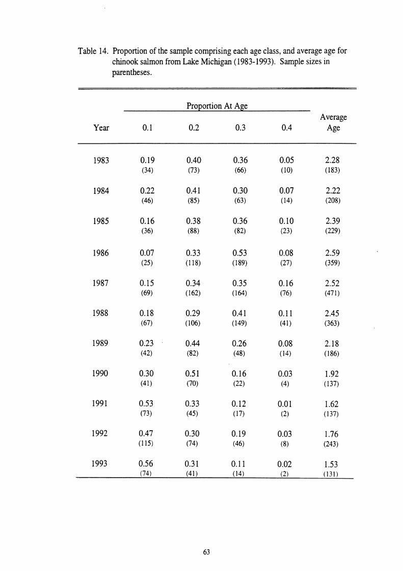
Table 14. Proportion of the sample comprising each age class, and average age for chinook salmon from Lake Michigan (1983-1993). Sample sizes in parentheses.
Proportion At Age Average
Year 0.1 0.2 0.3 0.4 Age

Table 15. Percent of sample with one year of stream residence, or of age 0.5 fish, based on the total sample of chinook salmon each year (1983-1993). Sample sizes in parentheses.
Age Type Sample
Year Size 1 .O 1.1 1.2 1.3 0.5
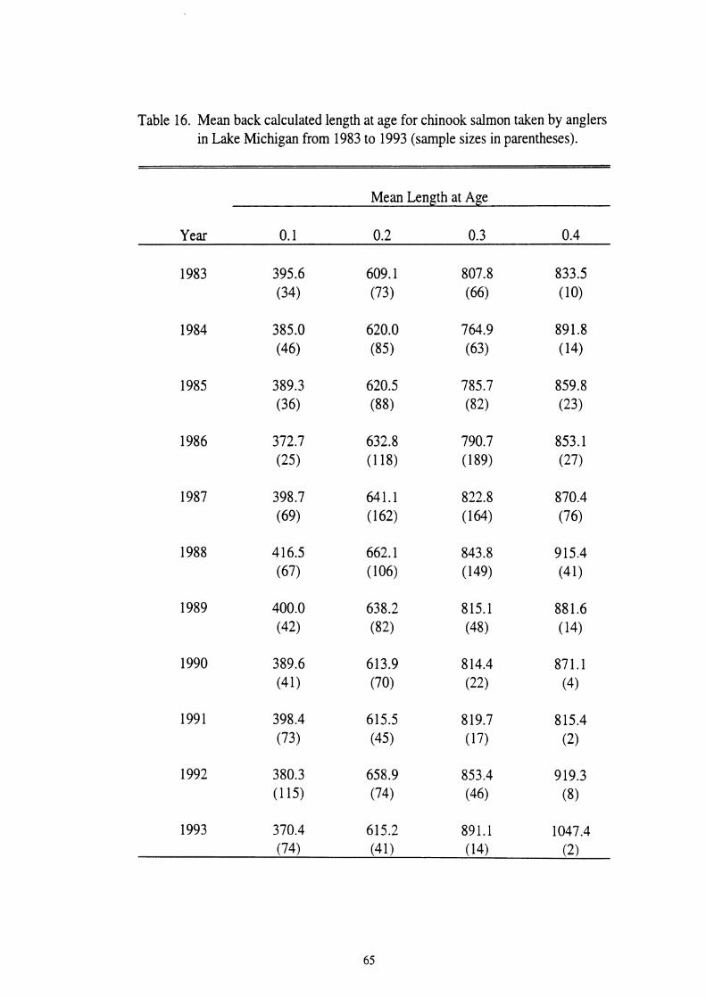
Table 16. Mean back calculated length at age for chinook salmon taken by anglers in Lake Michigan from 1983 to 1993 (sample sizes in parentheses).
Mean Length at Age
Year 0.1 0.2 0.3 0.4

Age 0.1
Age 0.2
Year of Harvest
Figure 15. Back calculated lengths of age 0.1 and 0.2 chinook salmon from Lake Michigan, 1983-1993. Means are represented by filled squares, brackets represent 95% confidence intervals. Sample size is below the x axis.

1983 to 1988, decreased from 1988 to 1990, increased from 1991 to 1992, and then
decreased from 1992 to 1993 (Figure 15; Mann-Whitney U; pc0.05).
Age 0.3 and 0.4 chinook salmon displayed significant annual differences in
back calculated length as well (ANOVA, pc0.05). Age 0.3 fish had a significant
decrease in back calculated length from 1983 to 1984 and an increase from 1984 to
1993 (Figure 16; Bonferroni Multiple Comparisons, pc0.05). Mean back calculated
length for age 0.4 fish increased from 1987 to 1988 and decreased in 199 1 despite the
low sample size (Figure 16; Bonferroni Multiple Comparisons, pc0.05).
Weight-length relationships were calculated for chinook salmon harvested in
spring (Table 17). Mean slope of the weight-length relationships before BKD (1983-
1987) was significantly lower (t-test, pc0.001) than the mean slope after BKD (1988-
1993) with values of 2.9891 and 3.2179, respectively. Predicted weights at age for
Lake Michigan chinook salmon are listed in Table 18. These weights have recent
decreasing trends for ages 0.1 and 0.2 from 1988 to 1993 (Mann-Whitney U,
p<0.001) with an increase in 1992 for age 0.2 (Mann-Whitney U, pc0.001). Age 0.3
significantly increased in weight from 1987 to 1993 (Mann-Whitney U, p=0.001), and
age 0.4 significantly increased in weight between 1987 and 1992 (Mann-Whitney U,
p=0.003).
.Age 0.1 and 0.2 fish exhibited significant differences in Fulton Index among
years (Table 19; Kruskal-Wallis, pc0.05) but had no consistent trends between 1983
and 1993 (Figure 17). There was a significant increase in Fulton Index in 1992 for
both ages, but mean condition decreased again in 1993 (Mann-Whitney U, p<0.05).

Age 0.3
Year of Harvest
1100.
1000'
900 '
800
700
Figure 16. Back calculated lengths of age 0.3 and 0.4 chinook salmon from Lake Michigan, 1983-1993. Means are represented by fdled squares, brackets represent 95% confidence intervals. Sample size is below the x axis.
I
Age 0.4
$1,
N= 10 14 23 27 76 41 14 4 2 8 2
1983 1984 1985 1986 1987 1988 1989 1990 1991 1992 1993
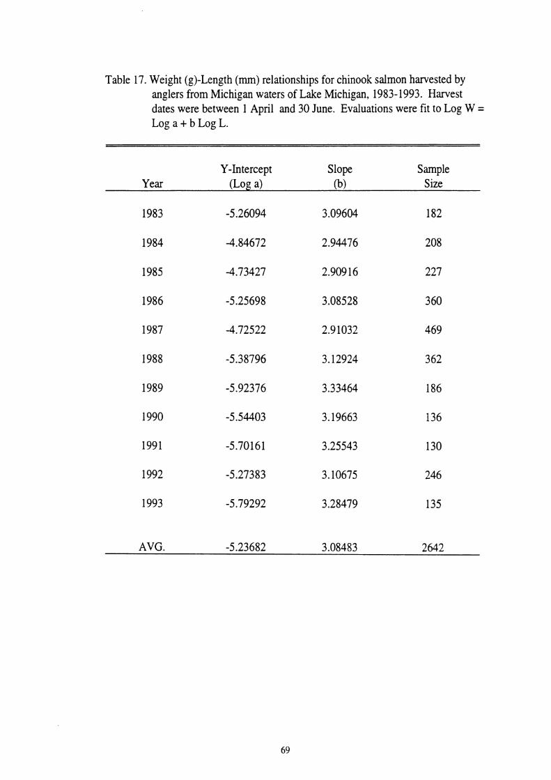
Table 117. Weight (g)-Length (rnrn) relationships for chinook salmon harvested by anglers from Michigan waters of Lake Michigan, 1983-1993. Harvest dates were between 1 April and 30 June. Evaluations were fit to Log W = Log a + b Log L.
Y-Intercept Slope Sample Year (Log a) (b) Size
AVG. -5.23682 3.08483 2642
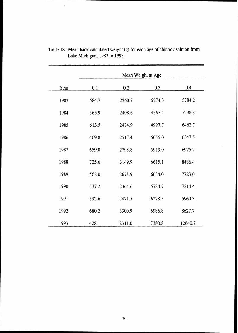
Table 18. Mean back calculated weight (g) for each age of chinook salmon from Lake Michigan, 1983 to 1993.
Mean Weight at Age
Year 0.1 0.2 0.3 0.4
1983 584.7 2260.7 5274.3 5784.2
1984 565.9 2408.6 4567.1 7298.3
1985 613.5 2474.9 4997.7 6462.7
1986 469.8 2517.4 5055.0 6347.5
1987 659.0 2798.8 5919.0 6975.7
1988 725.6 3 149.9 6615.1 8486.4
1989 562.0 2678.9 6034.0 7723.0
1990 537.2 2364.6 5784.7 72 14.4
1991 592.6 247 1.5 6278.5 5960.3
1992 680.2 3300.9 6986.8 8627.7
1993 428.1 231 1.0 7380.8 12640.7
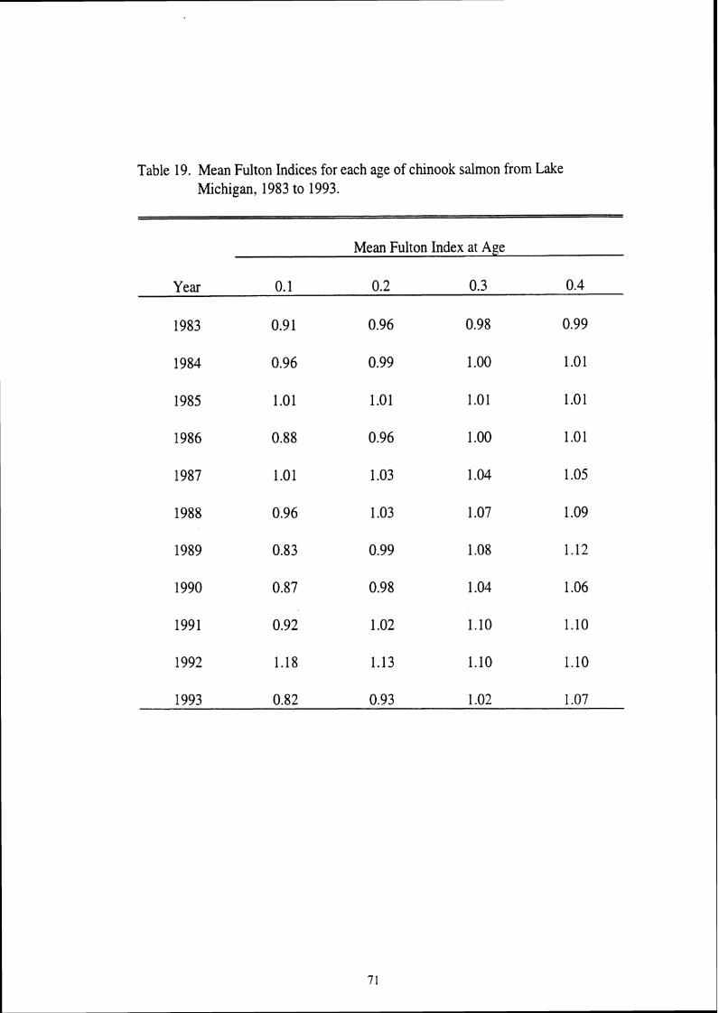
Table 19. Mean Fulton Indices for each age of chinook salmon from Lake Michigan, 1983 to 1993.
Mean Fulton Index at Age
Year 0.1 0.2 0.3 0.4
1983 0.9 1 0.96 0.98 0.99
1984 0.96 0.99 1.00 1.01
1 985 1.01 1.01 1.01 1.01
1986 0.88 0.96 1 .OO 1.01
11 987 1.01 1.03 1.04 1.05
1988 0.96 1.03 1.07 1.09
11989 0.83 0.99 1.08 1.12
1990 0.87 0.98 1.04 1.06

Age 0.1 -
Age 0.2 =
Year of Harvest
Figure 17. Fulton Indices of age 0.1 and 0.2 chinook salmon from Lake Michiam, 1983-1993. Means are represented by filled squares, brackets represent 95% confidence intervals. Sample size is below the x axis.

Age 0.3 and 0.4 condition also differed significantly among years (Kruskal-Wallis,
p<0.05). There was an increasing trend in condition for age 0.3 and 0.4 between1983
and 1993 (Figure 18). Mean Fulton Index increased by 0.062 for age 0.3 and 0.076
for age 0.4 after the onset of BKD based on the difference between the average
Fulton Index before and after 1988 for each age.
Age 0.1 chinook salmon achieved greater lengths (Table 20; F-test, p=0.02) in
the southern region of Lake Michigan than in the northern region. There were no
significant differences between regions for ages 0.2,0.3, or 0.4 (F-test, ~ ~ 0 . 0 5 ) .
Condition was significantly greater in the southern region for age 0.1 (F-test,
p<O.OOl), age 0.2 (Kruskal-Wallis, p<0.001), and age 0.3 (Kruskal-Wallis, p<0.001).
There was no significant difference in condition between the two regions for age 0.4
chinook salmon (F-test).
Discussion
Age 0.1 chinook salmon in Lake Michigan have decreased in growth between
1988 and 1993, while age 0.3 and 0.4 chinook salmon have increased in growth. The
increase in growth of ages 0.3 and 0.4 after BKD suggests that there was high
competition for food prior to BKD. Slow growth prior to BKD agrees with Hansen's
(1986) observation of a decrease in condition of chinook between 1969 and 1984
which he attributed to forage limitation. Bioenergetic models also predicted declines
of chinook salmon growth in Lake Michigan because of the reduction in adult alewife
biomass (Stewart et al. 1981, Stewart and Ibarra 1991).
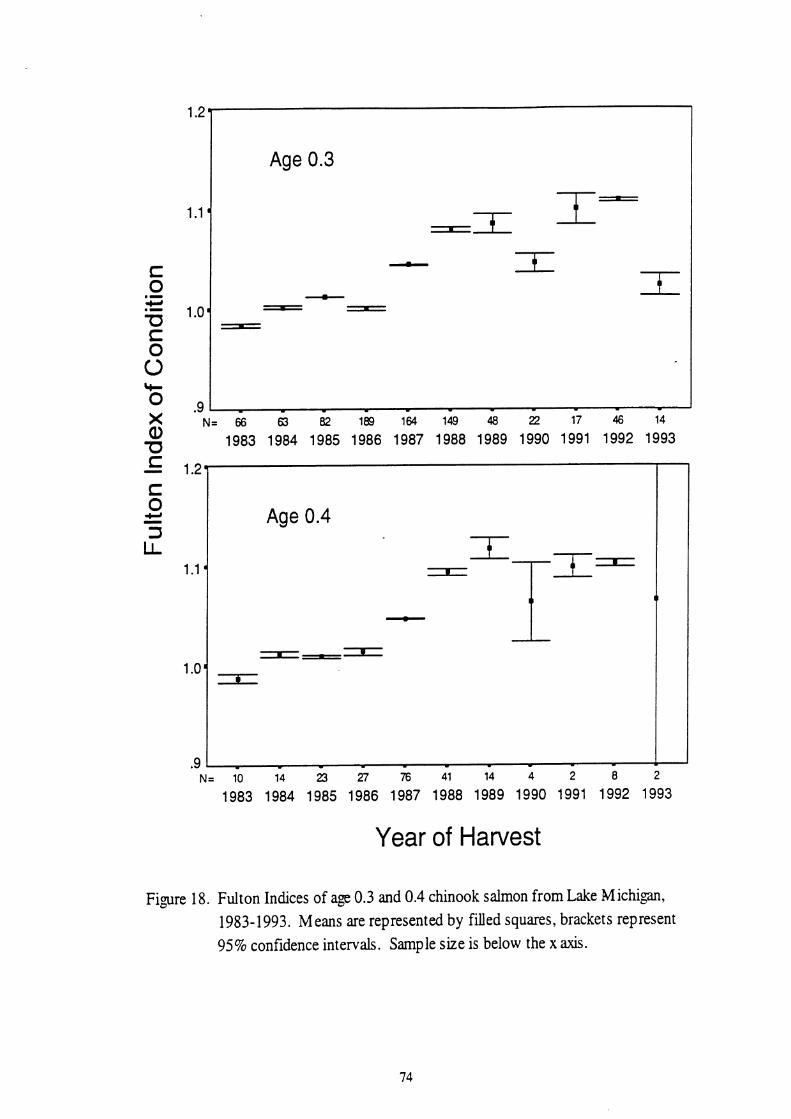
Year of Harvest
I .2
1.1 '
C 0 .I
-w .II 1.0' u s 0 0 + O .9 X
Figure 18. Fulton Indices of age 0.3 and 0.4 chinook salmon from Lake Michigin, 1983-1 993. Means are represented by filled squares, brackets represent 95% confidence intervals. Sample size is below the x axis.
Age 0.3
s I -
- Q)
N= 66 63 82 189 164 149 48 ZZ 17 46 14
u 1983 1984 1985 1986 1987 1988 1989 1990 1991 1992 1993 I= - 1.27 s 0 C, - 3 LL
1.1 '
1.0'
.9
Age 0.4
I
- 1.
I
a
N= 10 14 23 27 76 41 14 4 2 8 2
1983 1984 1985 1986 1987 1988 1989 1990 1991 1992 1993
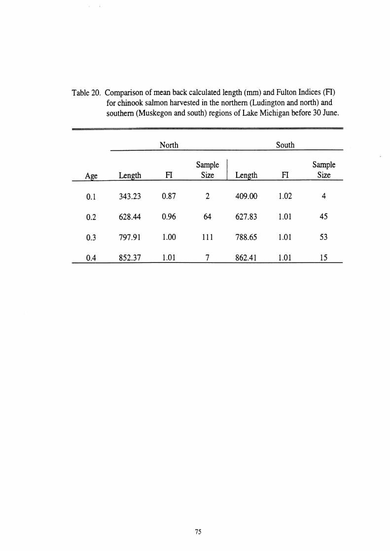
Table 20. Comparison of mean back calculated length (rnm) and Fulton Indices (FI) for chinook salmon harvested in the northern (Ludington and north) and southern (Muskegon and south) regions of Lake Michigan before 30 June.
North South
Sample Age Length FI Size
Sample Length FI Size
The increase in back calculated length and condition of age 0.3 and 0.4
chinook salmon after BKD may be associated with an intra-specific competitive
release, where by BKD caused sigruficant mortality and reduced the density of older
fish. With less competition for prey, age 0.3 and 0.4 chinook probably experienced
increased growth rates, which is supported by the increases in mean length and
condition. Density-dependent growth has been documented for kokanee salmon 0.
nerka (nonanadromous form) in Idaho reservoirs (Rieman and Myers 1992) and
sockeye salmon 0. nerka in Bristol Bay (Rogers 1980). Increased growth and
production as a response to reduced competition is well documented for fishes in the
genus Perca (Schneider and Crowe 1980, Hanson and Legget 1985, Persson 1986,
Hayes et al. 1992). The increase in growth may be compounded or explaind by the
possibility that fast growing fish survived BKD more often than slow growing fish,
increasing the frequency of these rapid growing fish in the population. Although
differential mortality based on size may be an alternative to the increase in growth
from competitive release, these hypotheses are not mutually exclusive.
Mean back calculated total length and condition decreased for age 0.1
chinook after BKD. This decline may have been due to a shift in fishing techniques to
smaller lure sizes (from plugs to spoons) allowing for more small chinook to be
harvested, it could also be due to a decline in forage abundance, or an increase in
abundance of age 0.1 chinook salmon due to additional stocking and natural
reproduction. Stocking of chinook salmon by Michigan increased 23% between 1987
and 1993, but overall stocking of chinook by all jurisdictions decreased by 30%
between 1989 and 1993 (Holey 1995). There were no major trends in age 0.2 lengths
and condition. Significant increases in condition for age 0.1 and age 0.2 fish in 1992
may be correlated to the warm spring that year (NOAA 1992).
The decrease in growth of age 0.1 may represent a critical period. If a
chinook salmon can achieve good growth through its first year, it may be able to
survive BKD, and then either live to an older age or mature at an earlier age. The
abundance of young-of-the-year and small alewife as forage and the abundance of
young chinook salmon may be affecting the growth of age 0.1 chinook salmon, but
the key may be the growth achieved between smoltification and age 0.1. In that case,
abundance of plankton and terrestrial invertebrates may be more important than
alewife. With recent invasions of Bythotrephes cederstroemii, a predatory
zooplankter (Lehman 1987), and zebra mussels Dreissena polymorpha, planktonic
invertebrates may have changed in species composition and numbers affecting both
young-of-the-year alewife and chinook salmon.
The last indication that there was a change in growth is the difference in slope
before and after the onset of BKD. A larger slope indicates an increase in condition
or more weight per given length. The mean slope before BKD was lower than the
mean slope after BKD. This suggests that condition, hence growth, was better after
1988 for the population. These slopes were based on spring lengths and weights so
there may be some variation between years due to temperature and other physical
factors. This index of growth also combined all ages so differences in growth by age
could not be determined.

The MDNR Creel Survey data also had several interesting age trends for
chinook salmon. The first was a decrease in the average age in the catch, where the
proportion of age 0.1 chinook increased and the proportion of age 0.3 and 0.4
chinook decreased from 1983-1993. The decrease in the proportion of age 0.3 and
0.4 chinook was undoubtedly due to high mortality from BKD. The increase in
number of age 0.1 chinook was probably due to the increase in stocking or natural
reproduction of chinook salmon in the Michigan waters of Lake Michigan. It may
also be due to the shift to smaller lure sizes by fishers and a shift to fishing over
deeper water where one-year-old chinook tend to inhabit (Elliott 1994). Perhaps the
appetite of the younger chinook also increased, making them more inclined to strike a
lure. Beukema (1968) found that starved threespine sticklebacks directed more
feeding attempts at inedible objects. The combination of using smaller lure sizes and
the increased attacks on lures due to hunger may have increased susceptibility of
younger chinook to the sport fishery.
The number of alternative age chinook salmon contributing to the sport
fishery varied from year to year. Fish spending one year in the stream contributed a
range of 0.0 % to 3.89 %. The greatest percent of stream yearlings was in 1992
which was a warm spring (NOAA 1992). A decrease in growth of smolts will
increase the number staying in the stream another year (Parker and Larkin 1959).
Therefore, the number of stream yearlings may be dependent on late winter and spring
physical conditions. This would explain the variability from year to year. Age 0.5
chinook were only observed in 1987 at 0.63 %. Since age at maturity is dependent on
growth (Parker and Larkin 1959, Healey 1986, Riddell 1986, Neilson and Geen
1986), this may indicate that growth was below normal because more fish delayed
reproduction (Mange1 1994). More age 0.4 and 0.5 chinook salmon contribute to the
sport fishery in Lake Superior (Berg 1978, Peck 1992) where low temperature and
production result in slower growth hence later age at maturity. However, age 0.5 fish
may also indicate better survival to reach older age. In any event, alternative ages of
chinook salmon contributed a low percentage to the total Lake Michigan sport
fishery.
Not only were there differences in age and growth between years, but there
were also differences in growth within years related to spring harvest location.
Assuming that chinook salmon harvested in a region of Lake Michigan before 30 June
resided in that region for the entire spring, then spring growth was better in the
southern compared to the northern part for younger fishes. Conditions of ages 0.1,
0.2 and 0.3 were also higher in chinook salmon harvested in the south compared to
the north. However, mean back calculated lengths were greater in the north for ages
0.2 and 0.3, and condition was greater in the north for age 0.4. The increase in spring
growth of chinook salmon in the south suggests that earlier warming of the water may
concentrate forage in that region, and that chinook salmon may benefit in the southern
region of the lake by foraging earlier in the spring. Larval fish may also become
available earlier for age 0.1 chinook salmon. However, the power of these data was
limited because there was a low sample size of age 0.1, and two years of data were
combined. Further support for increased growth benefits in southern Lake Michigan

would be the movement of the chinook sport fishery from south to north as the
summer progresses (Rakoczy and Svoboda 1994). Some of this northern migration
may be the return of mature salmon to their natal streams, and it may also be the
following of forage (Sornrners et al. 1981). Increasing temperatures and lake currents
(Ayers et al, 1958, Sato and Mortimer 1975) may also move forage and salmon north.
Was BKD caused by stress due to declines in forage abundance? There were
significant declines in condition for age 0.1 and 0.2 chinook salmon in 1986, prior to
the onset of BKD. This decrease in condition may indicate that stress caused the
initiation of BKD, and the evidence for improved growth in age 0.3 and 0.4 chinook
salmon after BKD indicates forage changes as the potential stress. Nonetheless, other
hypotheses for the BKD outbreak can not be ruled out. Using infected eggs and
sperm in hatcheries and stocking chinook at the same time sick fish are present in
shallow waters should still be considered as alternative hypothesis for the BKD
outbreak (Elliott 1994). A growth decline prior to the onset of BKD was also
indicated by the high proportion of older ages in the sport fishery in 1987, which
included the only year that 0.5-year-old fish were observed. Increased age at maturity
could signify decreased growth of the population.
Recognition of the changes in age and growth of chinook are important. The
reasons for the changes are difficult to answer due to the complexity of Lake
Michigan and the several changes that have occurred within it. The growth
compensation after BKD for age 0.3 and 0.4 and decreased condition of age 0.1 and
0.2 prior to BKD implicates that forage changes may have been limiting chinook

salmon in Lake Michigan. Therefore, the decrease in stocking of chinook salmon into
Lake Michigan is suggested to return historical growth rates and survival. Lower
stocking levels may allow alewife numbers to rebound providing better forage for
chinook salmon in the future and may restore the sport fishery for chinook salmon in
Lake Michigan.

APPENDICES

APPENDIX A
Table 2 1. Mean scale increment length (mm) for age 0.1 (focus to 1 st annulus), age 0.2 (1st to 2nd annulus), age 0.3 (2nd to 3rd annulus), and age 0.4 (3rd to 4th annulus) chinook salmon sport harvested from Lake Michigan, 1983- 1993.
Mean Scale Increment
'Year Age 0.1 Age 0.2 Age 0.3 Age 0.4
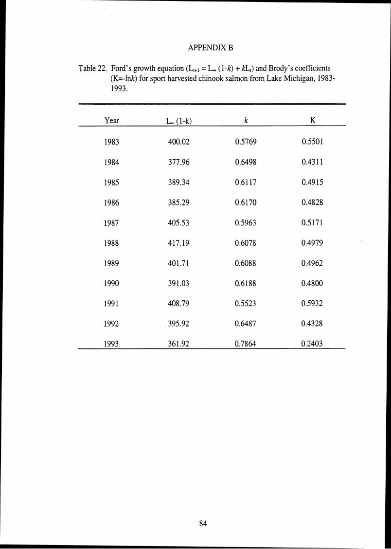
APPENDIX B
Table 22. Ford's growth equation (L,,, = L, (1 -k) t kLJ and Brody's coefficients (K=-lnk) for sport harvested chinook salmon from Lake Michigan, 1983- 1993.
- - - -- -
Year L, (I-k) k K
1983 400.02 0.5769 0.5501
1984 377.96 0.6498 0.43 1 1
1985 389.34 0.61 17 0.49 15
1986 385.29 0.6 170 0.4828
1987 405.53 0.5963 0.5171
1988 417.19 0.6078 0.4979
1989 401.7 1 0.6088 0.4962
1990 39 1.03 0.6 188 0.4800
1991 408.79 0.5523 0.5932
1992 395.92 0.6487 0.4328
1993 36 1.92 0.7864 0.2403

Literature Cited
Acker, C.J., and D. Mitchell. 1988. Jandel video analysis software manual, version 1.2. Jandel Scientific. Corte Madera, California. 26 1 p.
Anderson, R.O., and S.J. Gutreuter. 1983. Length, weight, and associated structural indices. Pages 283-300 in L.A. Nielson and D.L. Johnson, editors. Fisheries Techniques. American Fisheries Society, Bethesda, Maryland.
Anson, D. Personal communication. Michigan Department of Natural Resources, Plainwell, Michigan.
Appelget, J., and L.L. Smith, Jr. 1951. The determination of age and rate of growth from vertebrae of the channel catfish, Ictalurus lacustris punctatus. Transactions of the American Fisheries Society 80: 119-1 39.
Ayers, J.C., D.C. Chandler, G.H. Lauff, C.F. Powers, and E.B. Henson. 1958. Currents and water masses of Lake Michigan. University of Michigan Great Lakes Research Institute, Public Report No. 3. 169 p.
Bagenal, T.B., and F.W. Tesch, 1978. Age and growth. Pages 101-136 in T.B. Bagenal, editor. Methods for assessment of fish production in fresh waters. Blackwell Scientific Publications, Oxford.
Baker, T.T., and L.S. Tirnrnons. 199 1. Precision of ages estimated from five bony structures of Arctic char (Salvelinus alpinus) from the Wood River system, Alaska. Canadian Journal of Fisheries and Aquatic Sciences 48: 1007- 1014.
Beamish, R.J., and G.A. McFarlane. 1983. The forgotten requirements for age validation in fisheries biology. Transactions of the American Fisheries Society 1 12:735-743.
Becker, G.C. 1983. Fishes of Wisconsin. The University of Wisconsin Press, Madison. 1052 p.
Berg, R.E. 1978. Growth and maturation of chinook salmon, Oncorhynchus tshawytscha , introduced into Lake Superior. Transactions of the American Fisheries Society 107:28 1-283.
Beukema, J.J. 1968. Predation by the three-spined stickleback: the influence of hunger and experience. Behavior 3 1 : 1 - 126.

Bohlin, T., C. Dellefors, and U. Faremo. 1994. Probability of first sexual maturation of male parr in wild sea-run brown trout (Salmo trutta) depends on condition factor 1 year in advance. Canadian Journal of Fisheries and Aquatic Sciences 5 1 : 1920- 1926.
Brown, Jr., E.H., G.W. Eck, and C.O. Hatcher. 1994. Status of forage fish stocks in Lake Michigan, 1993. Great Lakes Fishery Commission Lake Michigan Committee Meeting, March 23-24, 1994, Ann Arbor. 232 p.
Carlander, K.D. 1949. Some considerations in the use of fish growth data based upon scale studies. Transactions of the American Fisheries Society 79: 187-194.
Carlander, K.D. 198 1. Caution on the use of the regression method of back- calculating lengths from scale measurements. Fisheries (Bethesda) 6(1): 2- 4.
Carlander, K.D. 1982. Standard intercepts for calculating lengths from scale measurements for some Centrarchid and Percid fishes. Transactions of the American Fisheries Society 11 1:332-336.
Carl, L.M. 1980. Aspects of the population ecology of chinook salmon in Lake Michigan tributaries. Doctoral dissertation, University of Michigan, Ann Arbor. 160 p.
Casselman, J.M. 1987. Determination of age and growth. Pages 209-242 in A.H. Weatherley and H.S. Gill, editors. The Biology of Fish Growth. Academic Press, London, England.
Chang, W.Y. 1982. A statistical method for evaluating the reproducibility of age determination. Canadian Journal of Fisheries and Aquatic Science 39: 1208-1210.
Chilton, D.E., and H.T. Bilton. 1986. New method for aging chinook salmon (Oncorhynchus tshawytscha) using dorsal fin rays, and evidence of its validity. Canadian Journal of Fisheries and Aquatic Sciences 43: 1588- 1594.
Diana, J.S. 1995. Biology and ecology of fishes. Biological Sciences Press, Carmel, Indiana. 441 p.

Elliott, R.F. 1994. Early life history of chinook salmon in Lake Michigan. Pages 286-308 in Anonymous, editor. Michigan sport fish restoration program annual reports for projects F-35-R-19 and F-53-R-10, April 1, 1993 to March 3 1, 1994. Michigan Department of Natural Resources, Fisheries Division, Lansing. 322 p.
Ferreira, B.P., and G.R. Russ. 1994. Age validation and estimation of growth rate of the coral trout, Plectropomus leopardus, from Lizard Island, Northern Great Barrier Reef. Fishery Bulletin 92:46-57.
Francis, R.I.C.C. 1990. Back-calculation of fish length: a critical review. Journal of Fish Biology 36:883-902.
Frost, W.E., and C. Kipling. 1980. The growth of charr, Salvelinus willughbii, in Windermere. Journal of Fish Biology 16:279-289.
Frie, R.V. 1982. Measurements of body lengths using a digitizing pad and microcomputer. Fisheries (Bethesda) 7(6):5-8.
Godfrey, H., D.D. Worlund, and H.T. Bilton. 1968. Tests on the accuracy of ageing chinook salmon (Oncorhynchus tshawytscha) from their scales. Journal of the Fisheries Research Board of Canada 25: 1971- 1982.
Hansen, M.J. 1986. Size and condition of trout and salmon from the Wisconsin waters of Lake Michigan, 1969-84. Wisconsin Department of Natural Resources, Fish Management Report 126, Madison.
Hanson, J.M., and W.C. Leggett. 1985. Experimental and field evidence for inter and intraspecific competition in two freshwater fishes. Canadian Journal of Fisheries and Aquatic Sciences 42:280-286.
Hard, J.J., A.C. Wertheimer, W.R. Heard, and R.M. Martin. 1985. Early male maturity in two stocks of chinook salmon (Oncorhynchus tshawytscha) transplanted to an experimental hatchery in southeastern Alaska. Aquaculture 48:35 1-359.
Harrison, E.J., and W.F. Hadley. 1979. A comparison of the use of cleithra to the use of scales for age and growth studies. Transactions of the American Fisheries Society 108:452-456.
Hartman, K.J., and F.J. Margraf. 1992. Effects of prey and predator abundance on prey consumption and growth of walleyes in western Lake Erie. Transactions of the American Fisheries Society 12 1 :245-260.

Hay, D.E., J.R. Brett, E. Bilinski, D.T. Smith, E.M. Donaldson, G.A. Hunter, and A.V. Solrnie. 1988. Experimental impoundments of prespawning Pacific herring (Clupea harengus): effects of feeding and density on maturation, growth, and proximate analysis. Canadian Journal of Fisheries and Aquatic Sciences 45:388-398.
Hay, R.L. 1992. Little Manistee River harvest weir and chinook salmon egg-take report, 1990. Michigan Department of Natural Resources, Fisheries Technical Report 92-5, Ann Arbor.
Hayes, D.B., W.W. Taylor, and J.C. Schneider. 1992. Response of yellow perch and benthic invertebrate community to a reduction in the abundance of white suckers. Transactions of the American Fisheries Society 121:36-53.
Healey, M.C. 199 1. Life history of chinook salmon. Pages 3 12-393 in C. Groot and L. Margolis, editors. Pacific salmon life histories. University of British Columbia Press, Vancouver.
Healey, M.C. 1986. Optimum size and age at maturity in Pacific salmon and effects of size-selective fisheries. Pages 39-52 in D.J.Meerburg, editor. Salmonid age at maturity. Canadian Special Publications of Fisheries and Aquatic Sciences 89, Ottawa.
Heath, D.D., J.W. Heath, and G.K. Iwama. 1991. Maturation in chinook salmon, Oncorhynchus tshawyrscha: early identification based on the development of a bimodal weight-frequency distribution. Journal of Fish Biology 39: 565-575.
Hesse, J.A. 1994. Contribution of hatchery and natural chinook salmon to the eastern Lake Michigan sport fishery, 1992-1993. Masters Thesis, Michigan State University, East Lansing. 82 p.
Hile, R. 1970. Body-scale relation and calculation of growth in fishes. Transactions of the American Fisheries Society 99:468-474.
Holey, M.E. 1995. Summary of trout and salmon stoclung in Lake Michigan 1976-1994. Great Lakes Fishery Commission Lake Michigan Committee Meeting, March 29-30, 1995. Milwaukee. 306 p.
Houthuijzen, R.P., J.J.G.M. Backx, and A.D. Buijse. 1993. Exceptionally rapid growth and early maturation of perch in a freshwater lake recently converted from an estruary. Journal of Fish Biology 43:320-324.

Jobling, M., and B.M. Baarduik. 199 1. Patterns of growth of maturing and immature Arctic charr, Salvelinus alpinus, in a hatchery population. Aquaculture 94:343-354.
Jobling, M., E.H. Jrzlrgensen, and S.I. Siikalvuopio. 1993. The influence of previous feeding regime on the compensatory growth response of maturing and immature Arctic charr, Salvelinus alpinus. Journal of Fish Biology 43: 409-41 9.
Johnson, L. 1976. Ecology of arctic populations of lake trout, Salvelinus namaycush, lake whitefish, Coregonus clupeafomis, Arctic char, S. alpinus, and associated species in unexploited lakes of the Canadian Northwest Territories. Journal of the Fisheries Research Board of Canada 33:2459-2488.
Jones, M.L., J.F. Koonce, and R. O'Gorman. 1993. Sustainability of hatchery- dependent salmonine fisheries in Lake Ontario: the conflict between predator demand and prey supply. Transactions of the American Fisheries Society 122: 1002-101 8.
Keller, M., K.D. Smith, and R.W. Rybicki. 1990. Review of salmon and trout management in Lake Michigan. Michigan Department of Natural Resources, Fisheries Special Report No. 14, Ann Arbor.
Lagler, K.F. 1977. Freshwater fishery biology. WM. C. Brown Company, Dubuque, Iowa. 42 1 p.
LaLanne, J.J., and G. Safsten. 1969. Age determination from scales of chum salmon (Oncorhynchus keta). Journal of the Fisheries Research Board of Canada 26:67 1-68 1.
Lehman, J.T. 1987. Palearctic predator invades North American Great Lakes. Oecologia 74:478-480.
Maclean, D.G., and G. Yoder. 1970. Kidney disease among Michigan salmon in 1967. Progressive Fish-Culturist 32:26-30.
Mangel, M. 1994. Climate change and salmonid life history variation. Deep-Sea research I1 41 :75-106.
Matlock, G.C., R.L. Colura, A.F. Maciorowski, and L.W. McEachron. 1987. Use of on-going tagging programs to validate scale readings. Pages 279-286 in R.C. Summerfelt and G.E. Hall, editors. Age and growth of fish. Iowa State University Press, Ames.
Matuszek, J.E., B.J. Shuter, and J.M. Casselman. 1990. Changes in lake trout growth and abundance after introductions of cisco into Lake Opeongo, Ontario. Transcactions of the American Fisheries Society 119:718-729.
McConnell, W.J. 195 1. The opercular bone as an indicator of age and growth of the carp, Cyprinus carpio Linnaeus. Transactions of the American Fisheries Society 8 1 : 138-149.
Miranda, L.E., W.M. Wingo, R.J. Muncy, and T.P. Bates. 1987. Bias in growth estimates derived from fish collected by anglers. Pages 21 1-220 in R.C. Summerfelt and G.E. Hall, editors. Age and growth of fish. Iowa State University Press, Ames.
Neilson, J.D., and G.H. Geen. 1982. Otoliths of chinook salmon (Oncorhynchus tshawytscha): daily growth increments and factors influencing their production. Canadian Journal of Fisheries and Aquatic Sciences 39: 1340- 1347.
Neilson, J.D., and G.H. Geen. 1986. First year growth rate of Sixes River chinook salmon as inferred from otoliths: effects on mortality and age at maturity. Transactions of the American Fisheries Society 1 15:28-33.
Nelson, D.D., and J.G. Hnath. 1990. Lake Michigan chinook salmon mortality, 1989. Michigan Department of Natural Resources, Fisheries Technical Report 90-4, Ann Arbor.
NOAA. 1992. Climatological data annual summary, Michigan 107: 1-3 1.
Norusis, M.J. 1993. SPSS for windows: base system user's guide, release 6.0. SPSS Inc. Chicago, Illinois. 828 p.
Pannella, G. 197 1. Fish otoliths: daily growth layers and periodic patterns. Science 173:1124-1127.
Parsons, J.W. 1973. History of salmon in the Great Lakes, 1850-1970. U.S. Fish and Wildlife Service, Technical Paper 68, Washington, D.C.
Parker, R.R., and P.A. Larkin. 1959. A concept of growth in fishes. Journal of Fisheries Research Board of Canada 16:72 1-745.
Peck, J.W. 1992. The sport fishery and contribution of hatchery trout and salmon in Lake Superior and tributaries at Marquette, Michigan, 1984-87. Michigan Department of Natural Resources, Fisheries Research Report 1975, Ann Arbor.

Pecor, C.H. 1992. Platte River harvest weir and coho salmon egg-take report, 199 1. Michigan Department of Natural Resources, Fisheries Technical Report 92-3, Ann Arbor.
Persson, L. 1986. Effects of reduced interspecific competition on resource utilization in perch (Perca fluviatilis). Ecology 67: 355-364.
Pitt, T.K. 1975. Changes in abundance and certain biological characters of Grand Bank American plaice, Hippoglossoides platessoides. Journal of the Fisheries Research Board of Canada 32: 1388- 1398.
Prince, E.D., D.W. Lee, and J.C. Javech. 1985. Internal zonations in section of vertebrae from Atlantic bluefin tuna, Thunnus thynnus, and their potential use in age determination. Canadian Journal of Fisheries and Aquatic Sciences 42:938-946.
Quinn, T.P., and M.J. Unwin. 1993. Variation in life history patterns among New Zealand chinook salmon (Oncorhynchus rshawytscha) populations. Canadian Journal of Fisheries and Aquatic Sciences 50: 1414- 142 1 .
Rakoczy, G.P. 1992. Sportfishing catch and effort from the Michigan waters of Lake Michigan, Huron, Erie, and Superior, April 1, 1992-March 3 1, 1993. Michigan Department of Natural Resources, Fisheries Division, Technical Report 92-8, Ann Arbor.
Rakoczy, G.P., and R.F. Svoboda. 1994. Sportfishing catch and effort from the Michigan waters of Lake Michigan, Huron, Erie, and Superior, April 1, 1992-March 3 1, 1993. Michigan Department of Natural Resources, Fisheries Division, Technical Report 94-6, Ann Arbor.
heman, B.E., and D.L. Myers. 1992. Influence of fish density and relative productivity on growth of kokanee in ten oligotrophic lakes and reservoirs in Idaho. Transactions of the American Fisheries Society 12 1: 178-191.
Rein, T.A., and R.C. Bearnederfer. 1994. Accuracy and precision of white sturgeon age estimates from pectoral fin rays. Transactions of the American Fisheries Society 123:255-265.
hddell, B.E. 1986. Assessment of selective fishing on the age at maturity in Atlantic salmon (Salmo salar): a genetic perpective. Pages 102-109 in D.J. Meerburg, editor. Salmonid age at maturity. Canadian Special Publications in Fisheries and Aquatic Sciences 89, Ottawa.
Rogers, D.E. 1980. Density-dependent growth of Bristol Bay sockeye salmon. Pages 267-283 in Mcneil, W.J. and D.C. Himsworth, editors. Salmonid ecosystems of the North Pacific. Oregon State University Press, Corvallis.
Rybicki, R.W. 1994. Diet of chinook salmon in the Ludington-Pentwater area of Lake Michigan in 1993. Great Lakes Fishery Commission Lake Michigan Committee Meeting, March 23-24, 1994. Ann Arbor. 232 p.
Rybicki, R.W. 1995. Summary of chinook diet study in eastern Lake Michigan in 1994, Great Lakes Fishery Commission Lake Michigan Committee Meeting, Milwakee. 306 p.
Sato, G.K., and C.H. Mortimer. 1975. Lake currents and temperature near the western shore of Lake Michigan. Center for Great Lakes Studies, University of Wisconsin-Milwaukee, Special Report 22.
Scarnecchia, D.L. 1979. Variation of scale characteristics of coho salmon with sampling location on the body. Progressive Fish-Culturist 4 l(3): 132- 135.
Schneider, J.C., and W.R. Crowe. 1980. Effect of sucker removal on fish and fishing at Big Bear Lake. Michigan Department of Natural Resources, Fisheries Division, Research Report 1 883, Ann Arbor.
Seelbach, P.W., and G.B. Beyerle. 1984. Interpretation of the age and growth of anadromous salmonids using scale analysis. Michigan Department of Natural Resources, Fisheries Division, Technical Report 84-5, Ann Arbor.
Shafi, M., and B.M. Jasim. 1982. Some aspects of the biology of a cyprinid, Aspius vorax. Journal of Fish Biology 20:271-278.
Sharp, D., and D.R. Bernard. 1988. Precision of estimated ages of lake trout from five calcified structures. North American Journal of Fisheries Management 8:367-372.
Smith, S.H. 1968. Species succession and fishery exploitation in the Great Lakes. Journal of the Fisheries Research Board of Canada 25667-693.
Sommers, M.L, C. Thompson, S. Tainter, L. Lin, T.W. Colucci, and J.M. Lipsey. 198 1. Fish in Lake Michigan: distribution of selected species. Michigan Sea Grant Report 8 1-600, East Lansing.
Stewart, D.J., and M. Ibarra. 1991. Predation and production by salmonine fishes in Lake Michigan, 1978-1988. Canadian Journal of Fisheries and Aquatic Sciences 48:909-922.

Stewart, D.J., J.F. IQtchell, and L.B. Crowder. 1981. Forage fishes and their salmonid predators in Lake Michigan. Transactions of the American Fisheries Society 1 10:75 1-763.
Tesch, F.W. 1968. Age and growth. Pages 93-123 in W.E. Ricker, editor. Methods for assessment of fish production in fresh waters. Blackwell Scientific Publications, London, England.
Tody, H.W., and H.A. Tanner. 1966. Coho salmon for the Great Lakes. Michigan Department of Conservation, Fish Management Report No. 1, Lansing.
Trippel, E.A. 1993. Relations of fecundity, maturation, and body size of lake trout, and implications for management in Northwestern Ontario lakes. North American Journal of Fisheries Management 13:64-72.
Wallin, 0 . 1957. On the growth structure and developmental physiology of the scale of fishes. Institute of Freshwater Research, Drottingholm 38: 325- 447.
Weatherley, A.H., and H.S. Gill. 1987. The biology of fish growth. Academic press, London. 443 p.
Wootton, R.J. 1990. Ecology of teleost fishes. Chapman and Hall, London. 404 pi