First Solar - · PDF fileConsulting Engineers South ... First Solar Module 1 Module 2 Module 3...
30
First Solar Energy Yield Simulations Module Performance Comparison for Four Solar PV Module Technologies Issue 1 | 8 May 2015 This report takes into account the particular instructions and requirements of our client. It is not intended for and should not be relied upon by any third party and no responsibility is undertaken to any third party. Job number 224283-00 Arup (Pty) Ltd Reg. No. 1994/004081/07 Registered Firm Consulting Engineers South Africa 10 High Street Postnet Suite No.93 Private Bag X1 Melrose Arch Johannesburg 2076 South Africa
Transcript of First Solar - · PDF fileConsulting Engineers South ... First Solar Module 1 Module 2 Module 3...

First Solar
Energy Yield Simulations
Module Performance Comparison for Four Solar PV Module Technologies
Issue 1 | 8 May 2015
This report takes into account the particular
instructions and requirements of our client.
It is not intended for and should not be relied
upon by any third party and no responsibility
is undertaken to any third party.
Job number 224283-00
Arup (Pty) Ltd Reg. No. 1994/004081/07 Registered Firm Consulting Engineers South Africa
10 High Street
Postnet Suite No.93 Private Bag X1 Melrose Arch
Johannesburg 2076
South Africa

First Solar Energy Yield Simulations
Module Performance Comparison for Four Solar PV Module Technologies
| Issue 1 | 8 May 2015
R:\REN\REAL JOBS\242283-00 FIRST SOLAR ENERGY VERFICATION\4. INTDAT\4.4 REPORTS\YIELD COMPARISONS REPORTS REDACTED 08-05-2015\MODULE
PERFORMANCE COMPARISON FOR FOUR SOLAR PV MODULE TECHNOLOGIES 08-05-2015 - REDACTED EB.DOCX
Contents
Page
1 Introduction 3
2 Project Locations 3
3 Simulation Method 4
3.1 Simulation Software 4
3.2 Meteorological Data 5
4 Design Assumptions 8
4.1 Facility Specifications 8
4.2 Model Inputs 12
4.3 Model Outputs 19
5 Results and Conclusions 22
Appendices
Appendix A
Site Result Summary
Appendix B
Detailed Simulation Results

First Solar Energy Yield Simulations
Module Performance Comparison for Four Solar PV Module Technologies
| Issue 1 | 8 May 2015
R:\REN\REAL JOBS\242283-00 FIRST SOLAR ENERGY VERFICATION\4. INTDAT\4.4 REPORTS\YIELD COMPARISONS REPORTS REDACTED 08-05-2015\MODULE PERFORMANCE COMPARISON FOR
FOUR SOLAR PV MODULE TECHNOLOGIES 08-05-2015 - REDACTED EB.DOCX
Page B2
Executive Summary
Arup has been appointed by First Solar to carry out an independent module performance comparison between First Solar modules and three other module technologies. The energy yield assessment has been completed for a hypothetical PV power plant at three different locations in South Africa and for both a fixed-axis and single-axis tracking mounting system. The three locations are Upington, Bloemfontein and Vryburg, which are all located in high irradiation regions of the country.
The fundamental approach used in comparing the module performance of the four selected module technologies, listed in Table 1, was to keep the system design parameters constant as far as possible and to only consider variables which are pertinent to the specific module.
PV Modules Selected for Analysis
First Solar Module 1 Module 2 Module 3
Model Range First Solar Series
4™ Not disclosed
Not disclosed
Not disclosed
Model Number FS-4112A-2
Nominal Rated Power
(STC) [Wp] 112.5 310 310 310
Technology Thin-film Poly-crystalline Poly-crystalline Mono-crystalline
Table 1 PV Modules selected for analysis
The simulations were performed using PVSyst v6.34 software and considered the P50 energy yield probability for the first year of production.
Table 2 shows the overall results for all module technologies at all the locations for fixed-axis and single-axis tracking systems. The results show that the selected First Solar modules were estimated to produce the highest energy yield in all scenarios.
Average annual performance during year 1
First Solar –
Thin Film
Base Case
First Solar –
Thin Film
Excl. Spectral
Adjustment
Module 1 –
Poly c-Si
Module 2 –
Poly c-Si
Module 3 –
Mono c-Si
Blo
emfo
nte
in
Fixed Tilt Energy Yield kWh/kWp 2 033 2 035 1 972 1 967 2 021
PR % 84.2% 84.3% 81.7% 81.4% 83.7%
Tracking Energy Yield kWh/kWp 2 373 2 376 2 298 2 292 2 349
PR % 81.0% 81.1% 78.4% 78.2% 80.2%
Up
ing
ton
Fixed Tilt Energy Yield kWh/kWp 2 078 2 091 2 015 2 008 2 069
PR % 82.3% 82.8% 79.8% 79.5% 81.9%
Tracking Energy Yield kWh/kWp 2 472 2 486 2 388 2 378 2 448
PR % 79.5% 80.0% 76.8% 76.5% 78.7%
Vry
bu
rg
Fixed Tilt Energy Yield kWh/kWp 2 021 2 011 1 945 1 939 1 995
PR % 84.2% 83.7% 81.0% 80.8% 83.1%
Tracking Energy Yield kWh/kWp 2 384 2 374 2 293 2 286 2 345
PR % 80.9% 80.5% 77.8% 77.5% 79.5%
Table 2: Summary of average performance during the first year of operations

First Solar Energy Yield Simulations
Module Performance Comparison for Four Solar PV Module Technologies
| Issue 1 | 8 May 2015
R:\REN\REAL JOBS\242283-00 FIRST SOLAR ENERGY VERFICATION\4. INTDAT\4.4 REPORTS\YIELD COMPARISONS REPORTS REDACTED 08-05-2015\MODULE PERFORMANCE COMPARISON FOR
FOUR SOLAR PV MODULE TECHNOLOGIES 08-05-2015 - REDACTED EB.DOCX
Page B3
1 Introduction
Under the terms of our Technical Services Agreement with First Solar (the Client), Arup has been tasked by First Solar to carry out an independent module performance comparison between First Solar modules and three other module technologies (the make and model of these three modules is not disclosed in this report). The energy yield assessment has been completed for a hypothetical PV power plant in three different locations in South Africa and for both a fixed-axis and single-axis tracking mounting system.
This report summarises the methodology, assumptions, results and conclusions associated with the comparison.
2 Project Locations
The three locations considered in this analysis are Upington, Vryburg and Bloemfontein, which are situated in high irradiation regions within South Africa, as shown in Figure 1 below. These locations were identified by the Client and they represent a range of temperature conditions in peak irradiation areas.
Figure 1: Three project locations considered in the analysis

First Solar Energy Yield Simulations
Module Performance Comparison for Four Solar PV Module Technologies
| Issue 1 | 8 May 2015
R:\REN\REAL JOBS\242283-00 FIRST SOLAR ENERGY VERFICATION\4. INTDAT\4.4 REPORTS\YIELD COMPARISONS REPORTS REDACTED 08-05-2015\MODULE PERFORMANCE COMPARISON FOR
FOUR SOLAR PV MODULE TECHNOLOGIES 08-05-2015 - REDACTED EB.DOCX
Page B4
3 Simulation Method
The analysis comprised of 24 energy yield simulations where the P50 energy yield probability for the first year of production was considered for examination.
The fundamental approach to comparing the module performance of the four selected module technologies was to keep the system design parameters constant as far as possible and to only consider variables which are pertinent to the specific module.
The detailed inputs and result for each simulation are included in Appendix B.
3.1 Simulation Software
The simulation process was undertaken by Arup using the industry standard PVSyst V6.34 software package. Figure 2 below describes the simulation process which is followed by PVSyst in order to calculate the expected energy generated by the PV facility.
Figure 2: PVSyst simulation process

First Solar Energy Yield Simulations
Module Performance Comparison for Four Solar PV Module Technologies
| Issue 1 | 8 May 2015
R:\REN\REAL JOBS\242283-00 FIRST SOLAR ENERGY VERFICATION\4. INTDAT\4.4 REPORTS\YIELD COMPARISONS REPORTS REDACTED 08-05-2015\MODULE PERFORMANCE COMPARISON FOR
FOUR SOLAR PV MODULE TECHNOLOGIES 08-05-2015 - REDACTED EB.DOCX
Page B5
3.2 Meteorological Data
Arup has used Meteonorm version 7 to derive hourly irradiation and temperature readings for each site.
The Meteonorm data has been compared to the solar resource values from NASA-SSE, PVGIS-Helioclim and PVGIS-SAF databases in order to verify that the dataset is applicable to each site. Meteonorm data is gathered by interpolating results from records of the nearest weather stations, and using satellite data where weather station records are not available. NASA-SSE, PVGIS-Helioclim and PVGIS-SAF data is sourced from satellite records.
The periods over which solar weather data has been gathered for each source is as follows:
Meteonorm: 1986 - 2005
NASA-SSE: 1983 – 2005
PVGIS-Helioclim: 1985 – 2004
PVGIS-SAF: 1998-2005 and 2006-2010
All module technology simulations at each location utilised the same meteorological data file for consistency.
3.2.1 Global Horizontal Irradiation
The Global Horizontal Irradiation comparison between the three locations and four data resources is shown in the Table 3 below.
Annual Global Horizontal Irradiation (kWh/m2/)
Meteonorm 7 PVGIS-SAF Diff
(%) NASA SSE Diff (%) PVGIS-HC Diff (%)
Upington 2,283 2,290 0.3% 2,140 -6.2% 2,159 -5.4%
Vryburg 2,194 2,188 -0.3% 2,097 -4.4% 2,162 -1.4%
Bloemfontein 2,170 2,122 -2.2% 2,067 -4.7% 2,155 -0.7%
Table 3: Comparison of Meteonorm, PVGIS-SAF, NASA-SSE and PVGIS – Helioclim annual global horizontal irradiation data
The value for the annual global horizontal irradiation provided by Meteonorm for all locations is within 2.2% of PVGIS-SAF, 6.2% of NASA-SSE, and 5.4% of PVGIS-Helioclim data. These differences are within a reasonable range and the Meteonorm data is thus considered appropriate to be used for the yield simulation.
Arup have chosen to use the Meteonorm data for each yield simulation as it is considered to be a more robust data source, and the uncertainty associated with the global horizontal irradiation is considered to be less than for the other three data sources.
Figure 3 below shows the close correlation between Meteonorm 7 data and the other three sources for each location.

First Solar Energy Yield Simulations
Module Performance Comparison for Four Solar PV Module Technologies
| Issue 1 | 8 May 2015
R:\REN\REAL JOBS\242283-00 FIRST SOLAR ENERGY VERFICATION\4. INTDAT\4.4 REPORTS\YIELD COMPARISONS REPORTS REDACTED 08-05-2015\MODULE PERFORMANCE COMPARISON FOR
FOUR SOLAR PV MODULE TECHNOLOGIES 08-05-2015 - REDACTED EB.DOCX
Page B6
(a) Upington
(b) Vryburg
(c) Bloemfontein
Figure 3: Comparison of monthly irradiance data for Upington, Vryburg and Bloemfontein
0.0
50.0
100.0
150.0
200.0
250.0
300.0
Jan Feb Mar Apr May Jun Jul Aug Sep Oct Nov Dec
GH
I [W
/m2
]
Meteonorm 7 NASA SSE PVGIS-SAF PVGIS-HC
0.0
50.0
100.0
150.0
200.0
250.0
300.0
Jan Feb Mar Apr May Jun Jul Aug Sep Oct Nov Dec
GH
I [W
/m2
]
Meteonorm 7 NASA SSE PVGIS-SAF PVGIS-HC
0.0
50.0
100.0
150.0
200.0
250.0
300.0
Jan Feb Mar Apr May Jun Jul Aug Sep Oct Nov Dec
GH
I [W
/m2
]
Meteonorm 7 NASA SSE PVGIS-SAF PVGIS-HC

First Solar Energy Yield Simulations
Module Performance Comparison for Four Solar PV Module Technologies
| Issue 1 | 8 May 2015
R:\REN\REAL JOBS\242283-00 FIRST SOLAR ENERGY VERFICATION\4. INTDAT\4.4 REPORTS\YIELD COMPARISONS REPORTS REDACTED 08-05-2015\MODULE PERFORMANCE COMPARISON FOR
FOUR SOLAR PV MODULE TECHNOLOGIES 08-05-2015 - REDACTED EB.DOCX
Page B7
3.2.2 Temperature Data
The temperature data used in Arup’s yield analysis (Table 4) has been obtained from Meteonorm over a period of 10 years (2000 – 2009) and verified with NASA-SSE data. From the data provided, it can be seen that Upington has the highest annual average temperature of the three sites, followed by Vryburg and then Bloemfontein.
Meteonorm V7 (°C)
Month Upington Vryburg Bloemfontein
Jan 28.3 24.4 22.5
Feb 28.3 24.0 22.0
Mar 25.5 22.1 19.6
Apr 21.5 19.0 15.5
May 16.6 15.2 10.9
Jun 13.1 12.5 8.0
Jul 13.0 12.0 7.3
Aug 15.0 15.2 10.8
Sep 18.8 19.1 14.8
Oct 23.3 22.3 18.8
Nov 25.4 23.2 20.3
Dec 27.8 24.6 22.4
Year 21.4 19.5 16.1
Table 4: Temperature data for the three project locations

First Solar Energy Yield Simulations
Module Performance Comparison for Four Solar PV Module Technologies
| Issue 1 | 8 May 2015
R:\REN\REAL JOBS\242283-00 FIRST SOLAR ENERGY VERFICATION\4. INTDAT\4.4 REPORTS\YIELD COMPARISONS REPORTS REDACTED 08-05-2015\MODULE PERFORMANCE COMPARISON FOR
FOUR SOLAR PV MODULE TECHNOLOGIES 08-05-2015 - REDACTED EB.DOCX
Page B8
4 Design Assumptions
4.1 Facility Specifications
The technical specifications of the PV facility are described in the sections below under the subcategories of PV Modules, System Design Characteristics and Substructure Characteristics.
Full details for each individual simulation (excluding comparison module make and model information) as well as the PVSyst output report are included in Appendix B.
4.1.1 PV Module Characteristics
Table 5 provides the technical parameters for the four module technologies.
The First Solar module selected for the analysis was the 112.5Wp thin-film module, which was proposed by First Solar.
The module manufacturers for the other module technologies were preselected by First Solar and are typical suppliers in the market, which will be referred to as ‘Module 1’, ‘Module 2’ and ‘Module 3’.
Two poly-crystalline (‘Module 1’ and ‘Module 2’) and one mono-crystalline module (‘Module 3’) were selected from the current catalogues of the module suppliers. The nominal capacity of each of these technologies was selected as 310Wp based on module capacities currently being used in the local industry and what is available on the supplier databases.
PV Module Characteristics
First Solar –
Thin Film
Module 1 –
Poly c-Si
Module 2 –
Poly c-Si
Module 3 –
Mono c-Si
Model Range First Solar Series
4™ Not disclosed
Not disclosed
Not disclosed
Model Number FS-4112A-2
Nominal Rated Power
(STC) [Wp] 112.5 310 310 310
Sorting Tolerance 0-2.5W 0-3% 0-3% -3/+5%
Module Efficiency at
STC [%] 15.62 15.98 15.98 19.06
Temperature Power
Coefficient [%/°C] -0.34 -0.41 -0.42 -0.38
Table 5: PV Module Characteristics for the four module technologies

First Solar Energy Yield Simulations
Module Performance Comparison for Four Solar PV Module Technologies
| Issue 1 | 8 May 2015
R:\REN\REAL JOBS\242283-00 FIRST SOLAR ENERGY VERFICATION\4. INTDAT\4.4 REPORTS\YIELD COMPARISONS REPORTS REDACTED 08-05-2015\MODULE PERFORMANCE COMPARISON FOR
FOUR SOLAR PV MODULE TECHNOLOGIES 08-05-2015 - REDACTED EB.DOCX
Page B9
4.1.2 System Design Characteristics
The PV system was designed to maintain consistency of all system parameters across the four simulations as far as possible. Table 6 below shows the system design characteristics for each technology.
The inverter selection for all module simulations was predefined by First Solar as the 800kW SMA Sunny Central Inverter (SMA 800CP XT). SMA is a globally renowned inverter supplier and the selected model range is commonly used for local utility scale solar PV projects.
The total AC capacity was designed to be as close to 75MWac as possible. This resulted in an AC capacity of 75.2MWac based on the use of 94 inverters per project. The DC/AC Ratio was maintained at 1.12 for all simulations, resulting in a DC capacity of c. 84MWp.
The module-string configuration for each module choice was optimised so that the Open-Circuit Voltage (VOC) was as close to the maximum inverter input voltage of 1000V as possible. Note that this resulted in the number of modules per string for First Solar and ‘Module 3 – Monocrystalline’ modules being lower than that for ‘Module 1 – Polycrystalline’ and ‘Module 2 – Polycrystalline’ due to the higher Open-Circuit Voltages applicable to these modules.
System Design Characteristics
First Solar –
Thin Film
Module 1 –
Poly c-Si
Module 2 –
Poly c-Si
Module 3 –
Mono c-Si
Nominal
Capacity (DC)
[kWp]
84,000 83,997 83,997 84,001
Inverter
Capacity (AC)
[kW]
75,200
DC/AC Ratio 1.12
Number of PV
Modules 746,670 270,959 270,959 270,970
Number of
Inverters 94
Modules per
String 10 19 19 14
Open-circuit
Voltage (V) 952 973 959 986
Table 6: System Design Characteristics

First Solar Energy Yield Simulations
Module Performance Comparison for Four Solar PV Module Technologies
| Issue 1 | 8 May 2015
R:\REN\REAL JOBS\242283-00 FIRST SOLAR ENERGY VERFICATION\4. INTDAT\4.4 REPORTS\YIELD COMPARISONS REPORTS REDACTED 08-05-2015\MODULE PERFORMANCE COMPARISON FOR
FOUR SOLAR PV MODULE TECHNOLOGIES 08-05-2015 - REDACTED EB.DOCX
Page B10
4.1.3 Substructure Characteristics
Table 7 below shows the substructure characteristics for the fixed-axis and single-axis tracking substructures for all technologies at the various project locations.
Substructure Characteristics
Parameter Fixed Tilt Tracking
Orientation 0°
(North Facing)
0°
(North - South Axis)
Shading Limit Angle 23°
(At module tilt angle)
23°
(At a maximum module tilt
angle of 45°)
Module Tilt Angle:
- 45° to + 45°
- Bloemfontein 26°
- Upington 25°
- Vryburg 24°
(Optimized for site locations)
Module Layout 4 high in landscape 4 high in landscape
Backtracking Control -
Applied to all module
technologies except for First
Solar modules
Table 7: Substructure Characteristics
Shading Limit Angle: The row spacing (pitch) for each technology was chosen such that the shading limit angle for each system was uniform in order to normalise shading losses.
The shading limit angle, as shown in Figure 4, is the minimum angle of the sun from which mutual shading of PV sheds begins. This varies between different facilities due to land constraints, which may require that arrays are located closer together, and the requirements for electrical cable losses that would be too high with excessive row spacing. For the fixed-axis systems a shading limit angle of 23° has been selected. This is within the range of that used typically on utility scale projects in South Africa.
Figure 4: Calculation of shading limit angle1
For tracking systems, a shading limit of 23° was also used to determine the pitch by applying the angle to the tracking system at its maximum rotation of 45°. Similarly this angle has been selected by considering rotation angles typically used in the region.
Module Tilt: The PV module tilt angle for the fixed-axis systems was optimised for each site and kept constant for all modules technologies at each site. The optimisation process took into account the
1 Figure taken from PVSyst V6.34

First Solar Energy Yield Simulations
Module Performance Comparison for Four Solar PV Module Technologies
| Issue 1 | 8 May 2015
R:\REN\REAL JOBS\242283-00 FIRST SOLAR ENERGY VERFICATION\4. INTDAT\4.4 REPORTS\YIELD COMPARISONS REPORTS REDACTED 08-05-2015\MODULE PERFORMANCE COMPARISON FOR
FOUR SOLAR PV MODULE TECHNOLOGIES 08-05-2015 - REDACTED EB.DOCX
Page B11
point of maximum annual irradiation when considering the inter-row shading defined by the shading limit angle.
The tracking system rotation angle was specified by First Solar at -45° to 45° and maintained for all sites. This is a common range for tracking systems.
Module Layout: The module layout of an array influences the string layout, which plays a role in the simulation of the electrical loss due to shading2.
Typically in a fixed axis system, modules are positioned up to four modules in landscape or two modules in portrait. In this study all modules were modelled as four high in landscape, which is the common First Solar approach.
The tracking simulations have also been modelled as four high in landscape. This is used for First Solar, but is not common for other modules that generally use one in portrait or two in landscape. However, in terms of an energy yield analysis this approach is acceptable as backtracking controls are applied to the other PV technologies to prevent direct shading. This minimizes the electrical effect due to shading on the crystalline modules.
Backtracking: Backtracking is used to prevent direct shading on modules typically during the early morning and later afternoon hours. The process involves reducing the tilt angle of the modules to prevent shading. It is primarily beneficial to alleviate electrical effect losses in crystalline modules.
Thin film modules, such as First Solar, are not affected by the electrical effect when orientated correctly. Thus in this case the greatest energy yield can be obtained by excluding backtracking controls. Further details on the electrical effect and backtracking functionality are provided in sections 4.2.2.3 and 4.3.1 respectively.
2 See section 4.2.2.3 for a description of the electrical loss due to shading

First Solar Energy Yield Simulations
Module Performance Comparison for Four Solar PV Module Technologies
| Issue 1 | 8 May 2015
R:\REN\REAL JOBS\242283-00 FIRST SOLAR ENERGY VERFICATION\4. INTDAT\4.4 REPORTS\YIELD COMPARISONS REPORTS REDACTED 08-05-2015\MODULE PERFORMANCE COMPARISON FOR
FOUR SOLAR PV MODULE TECHNOLOGIES 08-05-2015 - REDACTED EB.DOCX
Page B12
4.2 Model Inputs
Table 8 below describes the modelling inputs used to perform the energy yield simulations for each of the module technologies. A detailed explanation of certain user-defined inputs is provided in the sections to follow.
Modelling Inputs
First Solar
Module 1 –
Poly c-Si
Module 2 –
Poly c-Si
Module 3 –
Mono c-Si
Incl
ined
Irra
dia
tio
n
Transposition
Model
Hay:
First Solar recommend using the Hay transposition model to convert from horizontal
irradiation to in-plane irradiation. The same model has been used for all module types
for consistency.
Sh
adin
g a
nd
Ref
lect
ion
Shading Model Shading model built in PVSyst as per system configuration.
Horizon shading
loss
Calculated in PVSyst v6.34
Horizon obtained from Meteonorm v7
Structure shading
loss Calculated in PVSyst v6.34
Reflection loss
(IAM factor)
Module specific
IAM profile
provided by the
manufacturer.
Module specific IAM
profile provided by
the manufacturer.
IAM bo parameter
0.04 applied in
PVSyst to generate
the IAM profile
based on
recommendation
from manufacturer.
Module specific
IAM profile
provided by the
manufacturer.
Soiling loss Consistent monthly soiling loss applied for each module type.
PV
Mo
du
les
Monthly spectral
adjustment
Monthly Spectral
Adjustment applied
as per First Solar
documentation PD-
5-423 REV 2.1 -
Module
Characterization
Energy Prediction
Adjustment for
Local Spectrum.
No adjustment applied as not part of manufacturer energy
modelling recommendations.

First Solar Energy Yield Simulations
Module Performance Comparison for Four Solar PV Module Technologies
| Issue 1 | 8 May 2015
R:\REN\REAL JOBS\242283-00 FIRST SOLAR ENERGY VERFICATION\4. INTDAT\4.4 REPORTS\YIELD COMPARISONS REPORTS REDACTED 08-05-2015\MODULE PERFORMANCE COMPARISON FOR
FOUR SOLAR PV MODULE TECHNOLOGIES 08-05-2015 - REDACTED EB.DOCX
Page B13
Modelling Inputs
First Solar
Module 1 –
Poly c-Si
Module 2 –
Poly c-Si
Module 3 –
Mono c-Si
PV
Mo
du
les
(Co
nt.
)
PV loss / gain due
to irradiance level Calculated in PVSyst v6.34
Thermal losses
Thermal loss factor
applied: 30.7 W/m2
Based on
recommendation of
manufacturer
Thermal loss factor
applied: 29.0 W/m2
Standard Assumption
Thermal loss factor
applied: 29.0 W/m2
Standard Assumption
Thermal loss factor
applied: 29.0 W/m2
Based on
recommendation of
manufacturer
Shadings : electrical
loss
No Electrical Effect
Applied.
Linear shading used
due to thin film
module
characteristics in
orientation.
80% Electrical Effect applied to account for shading of string
cells.
DC health factor
loss
-1%
Generic loss applied to account operational losses due to aspects such as faulty module
connections, blown fuses and defective modules.
Power sorting
tolerance
adjustment
+0.6%
Gain has been
applied due to
modules being
positively sorted
with a tolerance of
0-2.5W (0 - 2.2%).
+0.8%
Gain has been applied
due to modules being
positively sorted with
a tolerance of 0-3%.
+0.8%
Gain has been applied
due to modules being
positively sorted with
a tolerance of 0-3%.
0.5%
Gain has been
applied due to
modules having a
tolerance of +5/-3%
Module array
mismatch loss
-1%
Generic loss applied to account for modules with differing I-V curves.
DC Ohmic wiring
loss
-1.5%
Generic loss applied. String lengths would be different with different module types due
to the different open circuit voltage characteristics. However, for this analysis this has
been kept constant and is assumed to be a design specification.
AC
ele
ctri
cal
com
pon
ents
Inverter efficiency
loss
Calculated in PVSyst using inverter file created according to latest datasheet for SMA
800CP XT
AC Ohmic wiring
loss
-0.5%
Generic loss applied. Considered for this analysis to be a design specification.
Transformer
resistive loss
-1%
Generic loss applied as not affected by module choice.
Transformer iron
loss
-0.1%
Generic loss applied as not affected by module choice.
Op
erat
ion
al
Lo
sses
Grid curtailment Not considered
Self-consumption
580MWh
Approximated from specified inverter auxiliary consumption of 1900W at rated
capacity applied for 8 hours per day and night-time consumption of 100W applied for
16 hours.

First Solar Energy Yield Simulations
Module Performance Comparison for Four Solar PV Module Technologies
| Issue 1 | 8 May 2015
R:\REN\REAL JOBS\242283-00 FIRST SOLAR ENERGY VERFICATION\4. INTDAT\4.4 REPORTS\YIELD COMPARISONS REPORTS REDACTED 08-05-2015\MODULE PERFORMANCE COMPARISON FOR
FOUR SOLAR PV MODULE TECHNOLOGIES 08-05-2015 - REDACTED EB.DOCX
Page B14
Modelling Inputs
First Solar
Module 1 –
Poly c-Si
Module 2 –
Poly c-Si
Module 3 –
Mono c-Si
Plant availability Not considered
Grid availability Not considered
Deg
rad
atio
n
Ave Year 1
Degradation (i.e.
average of
degradation at start
and end of year)
0%
No degradation has
been applied during
year 1 as
manufacturer has
confirmed that this
has been taken into
account already in
the specified power
rating during.
This is consistent
with the
manufacturer
recommended
modelling
guidelines.
-1.3%
Generic average first
year degradation for
polycrystalline
modules has been
applied.
-1.3%
Generic average first
year degradation for
polycrystalline
modules has been
applied.
-0.16%
Based on reported
findings by
independent
consultant
commissioned by
manufacturer.
Table 8: Modelling inputs for PVSyst yield simulations
4.2.1 Shading and Reflection
4.2.1.1 Shading: PVSyst Model. Horizon and Structure
The shading model, created in PVSyst as a 3D model, is based on the substructure design of the PV system for each module technology at each location.
Potential horizon shading affects have been analysed using Meteonorm v7. It was found that there are no significant horizon shading losses at any of the sites.
4.2.1.2 Reflection Loss
Reflection losses are due to the incidence angle at which the sun is entering the atmosphere and striking the surface of the panel. At incidence angles which are not normal to the atmospheric layer or to the panel there will be a certain degree of reflectance. This loss is based on an Incidence Angle Modifier (IAM) for various angles, which is often estimated as follows:
𝐼𝐴𝑀 = 1 − 𝑏𝑜 (1
𝑐𝑜𝑠𝑖− 1)
First Solar, ‘Module 1 – Polycrystalline’ and ‘Module 3 – Monocrystalline’ have been contacted and provided predefined IAM factors, while ‘Module 2 – Polycrystalline’ has recommended a bo value of 0.04.

First Solar Energy Yield Simulations
Module Performance Comparison for Four Solar PV Module Technologies
| Issue 1 | 8 May 2015
R:\REN\REAL JOBS\242283-00 FIRST SOLAR ENERGY VERFICATION\4. INTDAT\4.4 REPORTS\YIELD COMPARISONS REPORTS REDACTED 08-05-2015\MODULE PERFORMANCE COMPARISON FOR
FOUR SOLAR PV MODULE TECHNOLOGIES 08-05-2015 - REDACTED EB.DOCX
Page B15
4.2.1.3 Soiling Loss
Soiling losses are dependent on the site conditions and the frequency that the modules will be cleaned. For this analysis, soiling losses have been estimated based on monthly precipitation levels. The precipitation values were obtained from Meteonorm v7 database and the resultant monthly soiling loss values were computed according to the loss scale shown in Table 9.
Monthly Precipitation
[mm]
Soiling Loss
0-20 3%
20-50 2%
>50 1%
Table 9: Soiling Loss Scale
Note that for the First Solar modules, a monthly spectral loss adjustment has been applied as a system input combined with the soiling loss since there is no specific input in PVSyst for this adjustment. The revised monthly soiling loss values are a sum of the monthly spectral loss and the monthly soiling loss. Further details of this process is described in section 4.2.2.1.
4.2.2 PV Modules
4.2.2.1 Monthly spectral adjustment
PV modules respond differently to different spectral distributions of irradiation. This spectral distribution is site specific and varies based primarily on the amount of water vapour in the atmosphere together with dust, ozone and other particles.
Modules are rated at Standard Test Conditions (STC), which assumes a standard spectral distribution defined by ASTM G1733. Thus the performance of modules under different spectral distributions (which occur in practice) will differ from these conditions.
First Solar have studied this effect and recommend a methodology for estimating adjustments due to the spectral distribution to model their modules more accurately (See modelling note below).
It is understood that this effect has less of an influence for crystalline modules and it is thus not deemed necessary to apply in the model. The crystalline manufacturers have not defined specific adjustments required for their modules.
Thus Arup have followed current module manufacturer applied spectral adjustments to the First Solar simulations as a base case and excluded these from the remaining crystalline modules. However, the First Solar results with the spectral adjustment removed are also presented as a sensitivity test.
3 ASTM G173 “Standard Tables for Reference Solar Spectral Irradiances: Direct Normal and Hemispherical on
37° Tilted Surface”

First Solar Energy Yield Simulations
Module Performance Comparison for Four Solar PV Module Technologies
| Issue 1 | 8 May 2015
R:\REN\REAL JOBS\242283-00 FIRST SOLAR ENERGY VERFICATION\4. INTDAT\4.4 REPORTS\YIELD COMPARISONS REPORTS REDACTED 08-05-2015\MODULE PERFORMANCE COMPARISON FOR
FOUR SOLAR PV MODULE TECHNOLOGIES 08-05-2015 - REDACTED EB.DOCX
Page B16
PVSyst modelling note:
The monthly spectral adjustment is applied to First Solar modules in accordance with the
modules deviation from site-specific spectral irradiance from STC. The adjustment is
known as a spectral shift factor (M) and it is approximated on a monthly basis from the
hourly relative humidity (RH) and ambient temperature values as prescribed in First
Solar’s documentation (PD-5-423 REV 2.1) entitled: Module Characterization Energy
Prediction Adjustment for Local Spectrum.
For use in PVSyst, the hourly shift factors are irradiance weighted and averaged for each
calendar month to yield aggregate monthly spectral shift factors. As per PVSyst loss
notation, positive M values denote a loss in energy due to spectrum while negative values
denote an energy gain. The monthly spectral shift factors are incorporated into PVSyst
with the monthly soiling loss values, calculated in the process described in section 4.2.1.3.
Once the monthly soiling loss and spectral shift values are added together, an adjustment
is made to the DC health (module quality) loss so that the most negative monthly
combined spectral and soiling loss value (if applicable) is zero. In this way, the criteria of a
non-negative soiling loss is maintained in PVSyst and the offsetting of the additional
spectral loss parameter is transferred to the DC health loss.
4.2.2.2 Thermal Loss
PV module performance decreases with increases in temperature. The loss is based on the module’s power temperature coefficient presented in Table 5 and the field thermal loss factor.
The thermal loss factor is the rate of module heat loss and is due to the effects of convection around the panels, which reduces the temperature of the modules and improves performance.
First Solar has recommended using a constant loss factor of 30.7 W/m2 for their modules. This is marginally greater than the PVSyst default of 29.0 W/m2 for “Free” mounted modules with air circulation. However, noting that this recommendation was based on comparisons with operational data4 and that thin-film modules are constructed differently to typical crystalline modules, the manufacturer’s recommendation was considered reasonable.
The manufacturer of ‘Module 3’ has recommended the use of the standard 29.0 W/m2 value with their modules and this has been maintained for ‘Module 1’ and ‘Module 2’.
4.2.2.3 Shading: Electrical Loss
Typical crystalline modules consist of a number of cells connected in series. The electrical effect is the loss that occurs when one or more of these cells experiences shading, which limits the current flow through all other cells in the series.
The effect of string shading is approximated in PVSyst by considering when a string of modules experiences shading. A shading loss modelled 100% “according to module strings” will provide the most conservative upper limit for shading losses whereas a shading loss model which measures the linear effect5 will represent a lower limit. Arup have applied a typical estimate of an 80% electric effect loss for the simulations of the alternative crystalline modules.
The electrical effect is not applicable to thin film modules, such as the First Solar modules, if they have been orientated correctly. These effectively consist of thin long cells running the entire width of the modules. Thus in landscape orientation each cell in the module has an equal amount
4 See First Solar’s documentation PD-5-301-04 SS v1.1 entitled “Series 4 System Parameter Specification for
PVSYST” 5 Linear effect refers to a linear relationship between the proportion a module is shaded and energy yield.

First Solar Energy Yield Simulations
Module Performance Comparison for Four Solar PV Module Technologies
| Issue 1 | 8 May 2015
R:\REN\REAL JOBS\242283-00 FIRST SOLAR ENERGY VERFICATION\4. INTDAT\4.4 REPORTS\YIELD COMPARISONS REPORTS REDACTED 08-05-2015\MODULE PERFORMANCE COMPARISON FOR
FOUR SOLAR PV MODULE TECHNOLOGIES 08-05-2015 - REDACTED EB.DOCX
Page B17
of shading i.e. there are no cells completely shaded, which are connected in series to cells that are not shaded. This means that the shading is linear and no additional electrical effect applies.
4.2.2.4 DC Health Loss
The DC Health Factor Loss is considered to be a steady-state performance loss, which accounts for faults such as:
Under-performing strings due to module connection issues;
Blown fuses;
Defective modules;
In-homogeneities due to temperature gradients; and
MPPT tracking efficiency on system performance.
The 1% DC Health factor loss was applied all module technologies, given that it is applicable to all types of PV modules.
4.2.2.5 Power Sorting tolerance adjustment
The power sorting tolerance adjustment was based on specifications from each module manufacturer on how modules are sorted according to a certain power margin.
This adjustment was applied to account for variances between the flashed DC capacity of the facility and the nominal capacity, as typically facilities with positively toleranced modules have a flashed DC capacity greater than the nominal capacity.
First Solar (0-2.5W), ‘Module 1’ (0-3%) and ‘Module 2’ (0-3%) use a positive power tolerance, while ‘Module 3’ (-3% to +5%) has a negative to positive tolerance scale that results in a ‘net positive’ tolerance.
The calculation of the power sorting tolerance adjustment has been estimated based on net power tolerance of the module reduced by a factor of 4/15, commonly used for modules as a default value in PVSyst.
4.2.2.6 DC Ohmic wiring loss
The total cable loss between the modules and inverters is related to cable length and thickness / type.
As discussed in section 4.1.2 the number of modules per string varies between each module type due to varying open-circuit voltage characteristics. In addition, due to the varying module efficiency, the array sizes differ as well as the overall size of the facility.
Thus if identical string and other DC cables were used for each configuration it is likely that the associated losses would differ.
In this analysis Arup has taken a simplified approach and assumed that each configuration is to be designed to a specified DC loss of 1.5%.
We note that this excludes economic considerations from the analysis, as cable thickness would likely vary between these configurations in order to meet the specification, and the cost of the cables is influenced by the cable size.

First Solar Energy Yield Simulations
Module Performance Comparison for Four Solar PV Module Technologies
| Issue 1 | 8 May 2015
R:\REN\REAL JOBS\242283-00 FIRST SOLAR ENERGY VERFICATION\4. INTDAT\4.4 REPORTS\YIELD COMPARISONS REPORTS REDACTED 08-05-2015\MODULE PERFORMANCE COMPARISON FOR
FOUR SOLAR PV MODULE TECHNOLOGIES 08-05-2015 - REDACTED EB.DOCX
Page B18
4.2.3 AC Electrical Components
4.2.3.1 AC Ohmic wiring loss
AC cable losses occur between the inverters and the point of utility connection. If uniform cables are used for each facility, the losses will likely differ due to the different size of each facility. However, this difference is likely to be relatively small.
Arup has taken the same approach as for the DC cable losses and applied a constant 0.5% AC loss, which was considered as a design specification.
4.2.3.2 Transformer losses
Standard estimates for the transformer iron eddy-current loss (0.1%) and resistive/inductive losses (1%) have been applied for all technologies.
4.2.4 Operational Losses
4.2.4.1 Self-consumption
Central inverters consume additional energy to power the auxiliary systems such as cooling fans. This is typically not included in the specified efficiency on the data sheet.
Arup have approximated the inverter self-consumption based on the operating information provided in the SMA 800CP XT datasheet. The total annual self-consumption was calculated based on 8 hours of operation at maximum self-consumption at 1900W during the day and 16 hours of night time self-consumption at 100W, which equates to 580MWh/year. This has been applied to all technologies.
Self-consumption from plant lighting, security, office power, and the tracking system, where applicable, are expected to be low comparatively and have not been considered in this analysis.
4.2.4.2 Degradation
First Solar have provided confirmation that the recorded capacity of each module includes the first year degradation. Thus degradation was excluded from the yield simulations of these modules.
The manufacturer of ‘Module 3 – Monocrystalline’ commissioned a report by an independent consultant, which indicates that these modules show minimal degradation at 6 months and relatively low degradation after one year of operation of 0.33%. Arup have used this result to apply a degradation of 0.16% as the average rate over the first year.
For typical polycrystalline modules such as those considered for ‘Module 1’ and ‘Module 2’, there are varying reports on the initial and annual degradation. Arup have previously obtained data from similar manufacturers that indicate degradation after the first year of operations to range between 1.5% and 4.5%, although the latter is conservative and significantly worse than that in the warranty (typically 2.5% after one year). Further references indicate degradation during the first year of between 1% and 3.5%7. Consequently, an average degradation of 1.3% was applied for the first year.
7 See for example:
Pingel et al, “Initial Degradation Of Industrial Silicon Solar Cells In Solar Panels”;

First Solar Energy Yield Simulations
Module Performance Comparison for Four Solar PV Module Technologies
| Issue 1 | 8 May 2015
R:\REN\REAL JOBS\242283-00 FIRST SOLAR ENERGY VERFICATION\4. INTDAT\4.4 REPORTS\YIELD COMPARISONS REPORTS REDACTED 08-05-2015\MODULE PERFORMANCE COMPARISON FOR
FOUR SOLAR PV MODULE TECHNOLOGIES 08-05-2015 - REDACTED EB.DOCX
Page B19
4.3 Model Outputs
The following sections discuss specific system performance outputs calculated in PVSyst for all the simulations.
A summary of the outputs for each site is included in Appendix A and full results for each simulation are included in Appendix B.
4.3.1 Shading
The system performance affected by shading is based on the structure shading loss as well as the electrical loss due to shading. The structure shading loss is calculated by PVSyst by simulating the motion of the sun in hourly time-steps. This is a simple geometric calculation which will determine which portions of the arrays are in shade during each time step.
Fixed axis: When considering the calculated loss results of fixed-axis systems, there is a constant structure shading loss across all the technologies for each site. This is expected as a constant shading angle was applied to all systems8.
The electrical loss due to shading for the fixed tilt systems is a relatively minor loss (0.1% - 0.2%) and is only applicable for ‘Module 1’, ‘Module 2’ and ‘Module 3’ modules. As discussed above9, First Solar modules orientated correctly are not subject to electrical shading.
Single axis tracking: Backtracking controls were applied to the crystalline module simulations, which actively minimises losses due to direct shading. The single axis tracker follows the angle of the sun, but when the sun is at lower angles and mutual shading of each row would typically occur, the tracking system reduces the angle of all modules.
This removes losses due to direct shading and results in zero electrical loss for all module technologies. However, the modules are still partially shaded from the diffuse portion of irradiance; thus a structure shading loss occurs.
First Solar modules do not use backtracking controls, which results in greater losses due to structure shading than with the crystalline modules.
4.3.2 PV loss/gain due to irradiance level
The conversion efficiency of a PV module reduces at low light intensities and increases at higher light intensities. There is therefore a loss/gain in output of a module in practice compared with the standard irradiance conditions the modules are tested at (1,000 W/m2). This loss/gain depends on the characteristics of the module and the intensity of the incident irradiance in the field. PVSyst calculates the irradiance level loss/gain based on the information contained in the PV module data sheet.
For fixed-axis systems, the PV loss/gain due to irradiance level ranged from 0.1% gain to a loss of 0.4%. For single-axis tracking system the loss/gain was expectedly higher due to the higher incident irradiance and ranged from 0.2% gain to 0.3% loss. The First Solar modules
Coello, 2011, “Degradation Of Crystalline Silicon Modules: A Case Study On 785 Samples After Two Years Under
Operation”;
Makrides et al, 2010, “Degradation Of Different Photovoltaic Technologies Under Field Conditions”. 8 See section 4.1.3 9 See section 4.2.2.3

First Solar Energy Yield Simulations
Module Performance Comparison for Four Solar PV Module Technologies
| Issue 1 | 8 May 2015
R:\REN\REAL JOBS\242283-00 FIRST SOLAR ENERGY VERFICATION\4. INTDAT\4.4 REPORTS\YIELD COMPARISONS REPORTS REDACTED 08-05-2015\MODULE PERFORMANCE COMPARISON FOR
FOUR SOLAR PV MODULE TECHNOLOGIES 08-05-2015 - REDACTED EB.DOCX
Page B20
experienced the highest gain due to the irradiance level; whereas ‘Module 3’ modules had the greatest loss for all simulations.
4.3.3 Thermal Losses
The range of temperatures that modules experience during a year is heavily dependent on the range of ambient temperatures at a site.
Upington has the highest average temperature of all three test sites with a yearly average ambient temperature of 21.4 °C, followed by Vryburg (19.5 °C) and then Bloemfontein (16.1 °C). As expected, the thermal losses of all module technologies were greatest in test sites with higher temperatures.
Furthermore the thermal losses experienced by the modules in the single axis tracking facilities was marginally greater than the fixed tilt equivalents. This was also an expected trend as modules in tracking systems receive more irradiation and therefore heat, compared to fixed-axis systems; leading to an increased thermal loss.
In the simulations, the First Solar modules experienced the lowest thermal losses across all three locations in both fixed and tracking systems, which is expected due to the lower temperature power loss coefficient. ‘Module 3’ performed next best in all configurations, followed by ‘Module 1’ and then ‘Module 2’ modules.
4.3.4 Inverter Performance
The SMA 800CP XT inverter was used in all simulations. This resulted in a uniform loss of 1.5% annually for each technology, configuration and site.
When the string power increases above the inverter threshold on the I-V curve, there is an additional loss referred to as inverter loss over nominal power present. For each site this varied between the different module technologies. The modules with the greatest power output experienced the highest losses. This was expected as the same proportion of nominal DC module power to AC inverter power was applied across technologies.
The greatest inverter loss over nominal power losses were experienced by the tracking systems. This was expected as in these simulations the power output of each module string was greater than the fixed tilt scenarios.
4.3.5 DC Ohmic Wiring Loss
All modules were simulated with a 1.5% DC Ohmic wiring loss input, which is applicable at
STC conditions (1000W/m2 and 25°C). The simulated output loss of all modules was the same
for all fixed-axis systems with each showing a 1.2% loss across all locations.
There was a slight variance for the single-axis tracking systems results. The losses varied marginally from 1.3% to 1.4% amongst the modules technologies and locations. This is likely due to minor rounding errors in the simulation.
4.3.6 AC Ohmic Wiring Loss
All modules were simulated with a 0.5% AC Ohmic wiring loss input, which is applicable at
STC conditions (1000W/m2 and 25°C). The simulated output loss of all the modules was the
same for all Fixed Tilt systems with each showing a 0.3 % loss across all locations.

First Solar Energy Yield Simulations
Module Performance Comparison for Four Solar PV Module Technologies
| Issue 1 | 8 May 2015
R:\REN\REAL JOBS\242283-00 FIRST SOLAR ENERGY VERFICATION\4. INTDAT\4.4 REPORTS\YIELD COMPARISONS REPORTS REDACTED 08-05-2015\MODULE PERFORMANCE COMPARISON FOR
FOUR SOLAR PV MODULE TECHNOLOGIES 08-05-2015 - REDACTED EB.DOCX
Page B21
There was a slight variance for the single-axis tracking system results. First Solar showed a 0.4%
loss for all tracking systems across all locations. This was matched by ‘Module 3’ which also
showed a 0.4% loss for all tracking systems in all locations. ‘Module 1’ and ‘Module 2’ modules
maintained a constant 0.3% loss for all tracking systems in all locations. Similarly to the DC
loss, these are minor rounding errors in the calculation and should not have a material effect on
the results.

First Solar Energy Yield Simulations
Module Performance Comparison for Four Solar PV Module Technologies
| Issue 1 | 8 May 2015
R:\REN\REAL JOBS\242283-00 FIRST SOLAR ENERGY VERFICATION\4. INTDAT\4.4 REPORTS\YIELD COMPARISONS REPORTS REDACTED 08-05-2015\MODULE PERFORMANCE COMPARISON FOR
FOUR SOLAR PV MODULE TECHNOLOGIES 08-05-2015 - REDACTED EB.DOCX
Page B22
5 Results and Conclusions
Table 10 and Figures 5 to 7 below summarize the simulation results for the first year of production, across all sites, substructure configurations (fixed-axis or single-axis tracking) and module technologies. Further detailed comparisons are shown on a site by site basis in Appendix A and on a per simulation basis in Appendix B.
The table presents the specific yield, as well as the Performance Ratio (PR). Note that for the tracking systems the PR was calculated for all technologies using the in-plane irradiation excluding backtracking (ideal angles) for consistency.
Average annual performance during year 1
First Solar –
Thin Film
Base Case
First Solar –
Thin Film
Excl. Spectral
Adjustment
Module 1 –
Poly c-Si
Module 2 –
Poly c-Si
Module 3 –
Mono c-Si
Blo
emfo
nte
in
Fixed Tilt
Energy Yield kWh/kWp 2 033 2 035 1 972 1 967 2 021
PR % 84.2% 84.3% 81.7% 81.4% 83.7%
Variance % - 0.1% -3.0% -3.2% -0.6%
Tracking
Energy Yield kWh/kWp 2 373 2 376 2 298 2 292 2 349
PR % 81.0% 81.1% 78.4% 78.2% 80.2%
Variance % - 0.1% -3.1% -3.4% -1.0%
Up
ing
ton
Fixed Tilt
Energy Yield kWh/kWp 2 078 2 091 2 015 2 008 2 069
PR % 82.3% 82.8% 79.8% 79.5% 81.9%
Variance % - 0.6% -3.0% -3.4% -0.4%
Tracking
Energy Yield kWh/kWp 2 472 2 486 2 388 2 378 2 448
PR % 79.5% 80.0% 76.8% 76.5% 78.7%
Variance % - 0.6% -3.4% -3.8% -1.0%
Vry
bu
rg Fixed Tilt
Energy Yield kWh/kWp 2 021 2 011 1 945 1 939 1 995
PR % 84.2% 83.7% 81.0% 80.8% 83.1%
Variance % - -0.5% -3.8% -4.1% -1.3%
Tracking
Energy Yield kWh/kWp 2 384 2 374 2 293 2 286 2 345
PR % 80.9% 80.5% 77.8% 77.5% 79.5%
Variance % - -0.4% -3.8% -4.1% -1.6%
Table 10: Summary of results of Yield Analysis Simulations during year 1.The difference in energy yield
for each simulation compared to the First Solar base case is highlighted.
The year one results show that the First Solar modules had the highest estimated energy yield across all sites. The relative performance of these modules compared to the alternatives was greatest in the single axis tracking scenarios.
The simulation results of the First Solar modules without the spectral adjustment applied10 have also been shown as a sensitivity analysis. These indicate that applying the spectral adjustment decreases the estimate energy yield in certain locations (Bloemfontein and Upington), while increasing it in others (Vryburg) due to the differences in meteorological conditions at each site.
Note that for the scenarios tested, First Solar was estimated to have the highest estimated energy yield whether or not spectral adjustment was considered.
10 See section 4.2.2.1

First Solar Energy Yield Simulations
Module Performance Comparison for Four Solar PV Module Technologies
| Issue 1 | 8 May 2015
R:\REN\REAL JOBS\242283-00 FIRST SOLAR ENERGY VERFICATION\4. INTDAT\4.4 REPORTS\YIELD COMPARISONS REPORTS REDACTED 08-05-2015\MODULE PERFORMANCE COMPARISON FOR
FOUR SOLAR PV MODULE TECHNOLOGIES 08-05-2015 - REDACTED EB.DOCX
Page B23
Figure 5: Simulated performance in Bloemfontein during the first year of production.
75%
76%
77%
78%
79%
80%
81%
82%
83%
84%
85%
First Solar - Thin Film
Module 1 -Poly c-Si
Module 2 -Poly c-Si
Module 3 -Mono c-Si
Per
fro
man
ce R
atio
Bloemfontein - Performance Ratio (PR)
Fixed Tilt Tracking
1 000
1 250
1 500
1 750
2 000
2 250
2 500
Ener
gy Y
ield
[kW
h/k
Wp
]
Bloemfontein - Specific Yield
Fixed Tilt Tracking
First Solar - Thin Film
Module 1 -Poly c-Si
Module 2 -Poly c-Si
Module 3 -Mono c-Si

First Solar Energy Yield Simulations
Module Performance Comparison for Four Solar PV Module Technologies
| Issue 1 | 8 May 2015
R:\REN\REAL JOBS\242283-00 FIRST SOLAR ENERGY VERFICATION\4. INTDAT\4.4 REPORTS\YIELD COMPARISONS REPORTS REDACTED 08-05-2015\MODULE PERFORMANCE COMPARISON FOR
FOUR SOLAR PV MODULE TECHNOLOGIES 08-05-2015 - REDACTED EB.DOCX
Page B24
Figure 6: Simulated performance in Upington during the first year of production.
75%
76%
77%
78%
79%
80%
81%
82%
83%
84%
85%
Per
fro
man
ce R
atio
Upington - Performance Ratio (PR)
Fixed Tilt Tracking
1 000
1 250
1 500
1 750
2 000
2 250
2 500
Ener
gy Y
ield
[kW
h/k
Wp
]
Upington - Specific Yield
Fixed Tilt Tracking
First Solar - Thin Film
Module 1 -Poly c-Si
Module 2 -Poly c-Si
Module 3 -Mono c-Si
First Solar - Thin Film
Module 1 -Poly c-Si
Module 2 -Poly c-Si
Module 3 -Mono c-Si

First Solar Energy Yield Simulations
Module Performance Comparison for Four Solar PV Module Technologies
| Issue 1 | 8 May 2015
R:\REN\REAL JOBS\242283-00 FIRST SOLAR ENERGY VERFICATION\4. INTDAT\4.4 REPORTS\YIELD COMPARISONS REPORTS REDACTED 08-05-2015\MODULE PERFORMANCE COMPARISON FOR
FOUR SOLAR PV MODULE TECHNOLOGIES 08-05-2015 - REDACTED EB.DOCX
Page B25
Figure 7: Simulated performance in Vryburg during the first year of production.
75%
76%
77%
78%
79%
80%
81%
82%
83%
84%
85%
Per
fro
man
ce R
atio
Vryburg - Performance Ratio (PR)
Fixed Tilt Tracking
1 000
1 250
1 500
1 750
2 000
2 250
2 500
Ener
gy Y
ield
[kW
h/k
Wp
]
Vryburg - Specific Yield
Fixed Tilt Tracking
First Solar - Thin Film
Module 1 -Poly c-Si
Module 2 -Poly c-Si
Module 3 -Mono c-Si
First Solar - Thin Film
Module 1 -Poly c-Si
Module 2 -Poly c-Si
Module 3 -Mono c-Si

First Solar Energy Yield Simulations
Module Performance Comparison for Four Solar PV Module Technologies
| Issue 1 | 8 May 2015
R:\REN\REAL JOBS\242283-00 FIRST SOLAR ENERGY VERFICATION\4. INTDAT\4.4 REPORTS\YIELD COMPARISONS REPORTS REDACTED 08-05-2015\MODULE PERFORMANCE COMPARISON FOR
FOUR SOLAR PV MODULE TECHNOLOGIES 08-05-2015 - REDACTED EB.DOCX
Page B26
Appendix A
Site Result Summary

TITLE: Energy Yield Comparison Completed By: EB
SITE LOCATION: Bloemfontein Checked By: AB
Date: 15/05/08
REV: 1
Table 1: Comparison of system losses
First Solar –
Thin Film
First Solar –
Thin Film -
Excl Spectral
Module 1 -
Poly c-Si
Module 2 -
Poly c-Si
Module 3 –
Mono c-Si
First Solar –
Thin Film
First Solar –
Thin Film -
Excl Spectral
Module 1 -
Poly c-Si
Module 2 -
Poly c-Si
Module 3 –
Mono c-Si
[kWh/m2] 2 415 2 415 2 415 2 415 2 415 2 930 2 930 2 818 2 818 2 818
Horizon shading loss [%] 0.0% 0.0% 0.0% 0.0% 0.0% 0.0% 0.0% 0.0% 0.0% 0.0%
Structure shading loss [%] -2.1% -2.1% -2.1% -2.1% -2.1% -5.4% -5.4% -1.9% -1.9% -1.9%
Reflection loss (IAM factor) [%] -1.3% -1.3% -1.9% -2.0% -0.8% -0.6% -0.6% -1.3% -1.4% -0.4%
Soiling loss [%] -1.9% -1.9% -1.9% -1.9% -1.9% -1.7% -1.8% -1.8% -1.8% -1.8%
[kWh/m2] 2 289 2 289 2 274 2 273 2 301 2 709 2 705 2 682 2 678 2 704
[m2] 537 602 525 756 525 756 525 769 441 875 537 602 525 756 525 756 525 769 441 875
% 15.62% 15.98% 15.98% 15.98% 19.06% 15.62% 15.98% 15.98% 15.98% 19.06%
Array Nominal Energy [MWh] 192 257 192 208 191 061 190 962 193 865 227 443 227 129 225 280 225 059 227 751
Monthly Spectral Adjustment [%] -0.1% 0.0% 0.0% 0.0% 0.0% -0.1% 0.0% 0.0% 0.0% 0.0%
PV loss / gain due to irradiance level [%] 0.0% 0.0% 0.0% -0.1% -0.4% 0.1% 0.1% 0.0% 0.0% -0.3%
Thermal losses [%] -5.2% -5.3% -6.7% -6.9% -6.1% -5.8% -5.9% -7.6% -7.7% -6.8%
Shadings : Electrical Loss [%] 0.0% 0.0% -0.1% -0.1% -0.2% 0.0% 0.0% 0.0% 0.0% 0.0%
DC Health Factor Loss [%] -1.0% -1.0% -1.0% -1.0% -1.0% -1.0% -1.0% -1.0% -1.0% -1.0%
Power sorting tolerance adjustment [%] 0.6% 0.6% 0.8% 0.8% 0.5% 0.6% 0.6% 0.8% 0.8% 0.5%
Module array mismatch loss [%] -1.0% -1.0% -1.0% -1.0% -1.0% -1.0% -1.0% -1.0% -1.0% -1.0%
DC Ohmic wiring loss [%] -1.2% -1.2% -1.2% -1.2% -1.2% -1.3% -1.3% -1.3% -1.3% -1.3%
[MWh] 177 370 177 398 173 797 173 312 176 242 208 523 208 314 203 124 202 443 205 847
Inverter efficiency loss [%] -1.5% -1.5% -1.5% -1.5% -1.5% -1.5% -1.5% -1.5% -1.5% -1.5%
Inverter loss over nominal power [%] -0.5% -0.4% -0.2% -0.1% -0.3% -1.3% -1.0% -0.5% -0.4% -0.8%
AC Ohmic wiring loss [%] -0.3% -0.3% -0.3% -0.3% -0.3% -0.4% -0.4% -0.3% -0.3% -0.4%
Transformer resistive loss [%] -1.0% -1.0% -1.0% -1.0% -1.0% -1.0% -1.0% -1.0% -1.0% -1.0%
Transformer iron loss [%] -0.1% -0.1% -0.1% -0.1% -0.1% -0.1% -0.1% -0.1% -0.1% -0.1%
[MWh] 171 333 171 514 168 451 168 015 170 592 199 928 200 182 196 224 195 656 198 211
[%] 0.00% 0.00% 0.00% 0.00% 0.00% 0.00% 0.00% 0.00% 0.00% 0.00%
[%] 0.34% 0.34% 0.34% 0.34% 0.34% 0.29% 0.29% 0.29% 0.29% 0.29%
[%] 0.00% 0.00% 0.00% 0.00% 0.00% 0.00% 0.00% 0.00% 0.00% 0.00%
[%] 0.0% 0.00% 0.00% 0.00% 0.00% 0.00% 0.00% 0.00% 0.00% 0.00%
[MWh] 170 757 170 938 167 874 167 438 170 016 199 351 199 606 195 648 195 080 197 635
[kWh/kWp] 2 033 2 035 1 999 1 993 2 024 2 373 2 376 2 329 2 322 2 353
[%] 84.2% 84.3% 82.7% 82.5% 83.8% 81.0% 81.1% 79.5% 79.3% 80.3%
Table 2: Comparison of annual perfromance
First Solar –
Thin Film
First Solar –
Thin Film -
Excl Spectral
Module 1 -
Poly c-Si
Module 2 -
Poly c-Si
Module 3 –
Mono c-Si
First Solar –
Thin Film
First Solar –
Thin Film -
Excl Spectral
Module 1 -
Poly c-Si
Module 2 -
Poly c-Si
Module 3 –
Mono c-Si
[%] 0.00% 0.00% 1.32% 1.32% 0.16% 0.00% 0.00% 1.32% 1.32% 0.16%
[MWh] 170 757 170 938 165 658 165 228 169 744 199 351 199 606 193 065 192 505 197 319
[kWh/kWp] 2 033 2 035 1 972 1 967 2 021 2 373 2 376 2 298 2 292 2 349
[%] 84.16% 84.25% 81.65% 81.44% 83.66% 81.00% 81.10% 78.45% 78.22% 80.17%
[%] - -3.0% -3.2% -0.6% - -3.1% -3.4% -1.0%
[%] - -3.1% -3.3% -0.7% - -3.3% -3.6% -1.1%Rel Difference
(Specific Energy basis) - Excluding Spectral Adjustment
Average Degradation applied
Total energy injected into the grid
Specific energy injected into the grid
Performance Ratio
Rel Difference
(Specific Energy basis) - Including Spectral Adjustment
Specific energy injected into the grid
(excl. degradation)
Performance Ratio
(excl. degradation)
Average annual performance during year 1
Fixed Tilt Tracking
Total energy injected into the grid
(excl. degradation)
Irradiance on collectors
Total module area
Module Efficiency at STC
PV
Mo
du
les
Array Virtual energy at MPP
AC
ele
ctr
ical
co
mp
on
en
ts
Total energy excluding self consumption
Grid Curtailment Loss
Self Consumption Loss
Plant Availability Loss
Grid Availability Loss
Shad
ing
an
d
Refl
ecti
on
System performance calculations
Fixed Tilt Tracking
Annual irradiation in module plane
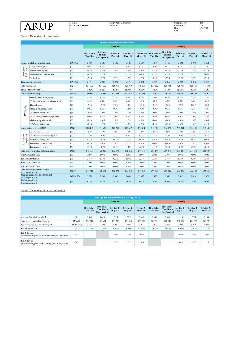
TITLE: Energy Yield Comparison Completed By: EB
SITE LOCATION: Upington Checked By: AB
Date: 15/05/08
REV: 1
Table 1: Comparison of system losses
First Solar –
Thin Film
First Solar –
Thin Film -
Excl Spectral
Module 1 -
Poly c-Si
Module 2 -
Poly c-Si
Module 3 –
Mono c-Si
First Solar –
Thin Film
First Solar –
Thin Film -
Excl Spectral
Module 1 -
Poly c-Si
Module 2 -
Poly c-Si
Module 3 –
Mono c-Si
[kWh/m2] 2 526 2 526 2 526 2 526 2 526 3 109 3 109 2 994 2 994 2 994
Horizon shading loss [%] 0.0% 0.0% 0.0% 0.0% 0.0% 0.0% 0.0% 0.0% 0.0% 0.0%
Structure shading loss [%] -1.8% -1.8% -1.8% -1.8% -1.8% -5.2% -5.2% -1.7% -1.7% -1.7%
Reflection loss (IAM factor) [%] -1.2% -1.2% -1.9% -2.0% -0.8% -0.5% -0.5% -1.1% -1.2% -0.4%
Soiling loss [%] -2.6% -2.5% -2.5% -2.5% -2.5% -2.5% -2.5% -2.5% -2.5% -2.5%
[kWh/m2] 2 388 2 388 2 374 2 371 2 401 2 859 2 859 2 837 2 834 2 858
[m2] 537 602 537 602 525 756 525 769 441 875 537 602 525 756 525 756 525 769 441 875
% 15.62% 15.62% 15.98% 15.98% 19.06% 15.62% 15.98% 15.98% 15.98% 19.06%
Array Nominal Energy [MWh] 200 515 200 555 199 405 199 243 202 235 240 122 240 050 238 362 238 104 240 800
Monthly Spectral Adjustment [%] -0.6% 0.0% 0.0% 0.0% 0.0% -0.6% 0.0% 0.0% 0.0% 0.0%
PV loss / gain due to irradiance level [%] 0.1% 0.1% 0.0% 0.0% -0.3% 0.2% 0.2% 0.2% 0.1% -0.2%
Thermal losses [%] -7.1% -7.1% -8.9% -9.1% -8.1% -7.6% -7.6% -9.7% -10.0% -8.8%
Shadings : Electrical Loss [%] 0.0% 0.0% -0.1% -0.1% -0.1% 0.0% 0.0% 0.0% 0.0% 0.0%
DC Health Factor Loss [%] -1.0% -1.0% -1.0% -1.0% -1.0% -1.0% -1.0% -1.0% -1.0% -1.0%
Power sorting tolerance adjustment [%] 0.6% 0.6% 0.8% 0.8% 0.5% 0.6% 0.6% 0.8% 0.8% 0.5%
Module array mismatch loss [%] -1.0% -1.0% -1.0% -1.0% -1.0% -1.0% -1.0% -1.0% -1.0% -1.0%
DC Ohmic wiring loss [%] -1.2% -1.2% -1.2% -1.2% -1.2% -1.3% -1.3% -1.4% -1.4% -1.3%
[MWh] 180 482 181 672 177 251 176 612 179 984 215 009 216 156 209 991 209 150 212 998
Inverter efficiency loss [%] -1.5% -1.5% -1.5% -1.5% -1.5% -1.5% -1.5% -1.5% -1.5% -1.5%
Inverter loss over nominal power [%] -0.1% -0.1% 0.0% 0.0% 0.0% -0.2% -0.2% -0.1% 0.0% -0.1%
AC Ohmic wiring loss [%] -0.3% -0.3% -0.3% -0.3% -0.3% -0.4% -0.4% -0.3% -0.3% -0.4%
Transformer resistive loss [%] -1.0% -1.0% -1.0% -1.0% -1.0% -1.0% -1.0% -1.0% -1.0% -1.0%
Transformer iron loss [%] -0.1% -0.1% -0.1% -0.1% -0.1% -0.1% -0.1% -0.1% -0.1% -0.1%
[MWh] 175 094 176 227 172 071 171 456 174 680 208 195 209 389 203 813 203 019 206 536
[%] 0.00% 0.00% 0.00% 0.00% 0.00% 0.00% 0.00% 0.00% 0.00% 0.00%
[%] 0.33% 0.33% 0.33% 0.34% 0.33% 0.28% 0.28% 0.28% 0.28% 0.28%
[%] 0.00% 0.00% 0.00% 0.00% 0.00% 0.00% 0.00% 0.00% 0.00% 0.00%
[%] 0.00% 0.00% 0.00% 0.00% 0.00% 0.00% 0.00% 0.00% 0.00% 0.00%
[MWh] 174 518 175 651 171 494 170 880 174 103 207 618 208 812 203 237 202 443 205 960
[kWh/kWp] 2 078 2 091 2 042 2 034 2 073 2 472 2 486 2 420 2 410 2 452
[%] 82.3% 82.8% 80.8% 80.5% 82.1% 79.5% 80.0% 77.8% 77.5% 78.9%
Table 2: Comparison of annual perfromance
First Solar –
Thin Film
First Solar –
Thin Film -
Excl Spectral
Module 1 -
Poly c-Si
Module 2 -
Poly c-Si
Module 3 –
Mono c-Si
First Solar –
Thin Film
First Solar –
Thin Film -
Excl Spectral
Module 1 -
Poly c-Si
Module 2 -
Poly c-Si
Module 3 –
Mono c-Si
[%] 0.00% 0.00% 1.32% 1.32% 0.16% 0.00% 0.00% 1.32% 1.32% 0.16%
[MWh] 174 518 175 651 169 230 168 624 173 825 207 618 208 812 200 554 199 770 205 630
[kWh/kWp] 2 078 2 091 2 015 2 008 2 069 2 472 2 486 2 388 2 378 2 448
[%] 82.25% 82.79% 79.77% 79.48% 81.93% 79.51% 79.97% 76.81% 76.51% 78.75%
[%] - -3.0% -3.4% -0.4% - -3.4% -3.8% -1.0%
[%] - -3.7% -4.0% -1.0% - -4.0% -4.3% -1.5%Rel Difference
(Specific Energy basis) - Excluding Spectral Adjustment
Annual irradiation in module plane
Sh
adin
g a
nd
Refl
ecti
on
Irradiance on collectors
Total module area
Module Efficiency at STC
Array Virtual energy at MPP
AC
ele
ctr
ical
co
mp
on
en
ts
Total energy excluding self consumption
Total energy injected into the grid
(excl. degradation)
Specific energy injected into the grid
(excl. degradation)
Plant Availability Loss
Self Consumption Loss
Grid Curtailment Loss
Rel Difference
(Specific Energy basis) - Including Spectral Adjustment
Performance Ratio
Average Degradation applied
Total energy injected into the grid
Specific energy injected into the grid
PV
Mo
du
les
System performance calculations
Fixed Tilt Tracking
Fixed Tilt Tracking
Average annual performance during year 1
Grid Availability Loss
Performance Ratio
(excl. degradation)

TITLE: Energy Yield Comparison Completed By: EB
SITE LOCATION: Vryburg Checked By: AB
Date: 15/05/08
REV: 1
Table 1: Comparison of system losses
First Solar –
Thin Film
First Solar –
Thin Film -
Excl Spectral
Module 1 -
Poly c-Si
Module 2 -
Poly c-Si
Module 3 –
Mono c-Si
First Solar –
Thin Film
First Solar –
Thin Film -
Excl Spectral
Module 1 -
Poly c-Si
Module 2 -
Poly c-Si
Module 3 –
Mono c-Si
[kWh/m2] 2 401 2 401 2 401 2 401 2 401 2 948 2 948 2 840 2 840 2 840
Horizon shading loss [%] 0.0% 0.0% 0.0% 0.0% 0.0% 0.0% 0.0% 0.0% 0.0% 0.0%
Structure shading loss [%] -1.9% -1.9% -1.9% -1.9% -1.9% -5.3% -5.3% -1.9% -1.9% -1.9%
Reflection loss (IAM factor) [%] -1.3% -1.3% -2.0% -2.0% -0.8% -0.6% -0.6% -1.2% -1.3% -0.4%
Soiling loss [%] -2.0% -2.0% -2.0% -2.0% -2.0% -1.8% -1.9% -1.9% -1.9% -1.9%
[kWh/m2] 2 278 2 278 2 263 2 261 2 290 2 726 2 723 2 701 2 898 2 722
[m2] 537 602 525 756 525 756 525 769 441 875 537 602 525 756 525 756 525 769 441 875
% 15.62% 15.98% 15.98% 15.98% 19.06% 15.62% 15.98% 15.98% 15.98% 19.06%
Array Nominal Energy [MWh] 191 306 191 257 190 124 190 013 192 919 228 882 228 613 226 911 226 725 229 340
Monthly Spectral Adjustment [%] 0.6% 0.0% 0.0% 0.0% 0.0% 0.5% 0.0% 0.0% 0.0% 0.0%
PV loss / gain due to irradiance level [%] 0.0% 0.0% 0.0% -0.1% -0.4% 0.1% 0.1% 0.1% 0.0% -0.3%
Thermal losses [%] -6.0% -6.1% -7.7% -7.9% -7.0% -6.7% -6.7% -8.6% -8.8% -7.7%
Shadings : Electrical Loss [%] 0.0% 0.0% -0.1% -0.1% -0.1% 0.0% 0.0% 0.0% 0.0% 0.0%
DC Health Factor Loss [%] -1.0% -1.0% -1.0% -1.0% -1.0% -1.0% -1.0% -1.0% -1.0% -1.0%
Power sorting tolerance adjustment [%] 0.6% 0.6% 0.8% 0.8% 0.5% 0.6% 0.6% 0.8% 0.8% 0.5%
Module array mismatch loss [%] -1.0% -1.0% -1.0% -1.0% -1.0% -1.0% -1.0% -1.0% -1.0% -1.0%
DC Ohmic wiring loss [%] -1.2% -1.2% -1.2% -1.2% -1.2% -1.3% -1.3% -1.3% -1.3% -1.3%
[MWh] 176 230 175 051 171 228 170 714 173 778 209 080 207 816 202 385 201 694 205 204
Inverter efficiency loss [%] -1.5% -1.5% -1.5% -1.5% -1.5% -1.5% -1.5% -1.5% -1.5% -1.5%
Inverter loss over nominal power [%] -0.4% -0.3% -0.1% -0.1% -0.2% -1.2% -0.9% -0.4% -0.3% -0.7%
AC Ohmic wiring loss [%] -0.3% -0.3% -0.3% -0.3% -0.3% -0.4% -0.4% -0.3% -0.3% -0.4%
Transformer resistive loss [%] -1.0% -1.0% -1.0% -1.0% -1.0% -1.0% -1.0% -1.0% -1.0% -1.0%
Transformer iron loss [%] -0.1% -0.1% -0.1% -0.1% -0.1% -0.1% -0.1% -0.1% -0.1% -0.1%
[MWh] 170 336 169 470 166 103 165 627 168 403 200 824 199 995 195 756 195 169 197 887
[%] 0.00% 0.00% 0.00% 0.00% 0.00% 0.00% 0.00% 0.00% 0.00% 0.00%
[%] 0.34% 0.34% 0.35% 0.35% 0.34% 0.29% 0.29% 0.29% 0.30% 0.29%
[%] 0.00% 0.00% 0.00% 0.00% 0.00% 0.00% 0.00% 0.00% 0.00% 0.00%
[%] 0.0% 0.00% 0.00% 0.00% 0.00% 0.00% 0.00% 0.00% 0.00% 0.00%
[MWh] 169 759 168 893 165 527 165 051 167 827 200 248 199 418 195 179 194 593 197 311
[kWh/kWp] 2 021 2 011 1 971 1 965 1 998 2 384 2 374 2 324 2 317 2 349
[%] 84.2% 83.7% 82.1% 81.8% 83.2% 80.9% 80.5% 78.8% 78.6% 79.7%
Table 2: Comparison of annual perfromance
First Solar –
Thin Film
First Solar –
Thin Film -
Excl Spectral
Module 1 -
Poly c-Si
Module 2 -
Poly c-Si
Module 3 –
Mono c-Si
First Solar –
Thin Film
First Solar –
Thin Film -
Excl Spectral
Module 1 -
Poly c-Si
Module 2 -
Poly c-Si
Module 3 –
Mono c-Si
[%] 0.00% 0.00% 1.32% 1.32% 0.16% 0.00% 0.00% 1.32% 1.32% 0.16%
[MWh] 169 759 168 893 163 342 162 872 167 558 200 248 199 418 192 603 192 024 196 995
[kWh/kWp] 2 021 2 011 1 945 1 939 1 995 2 384 2 374 2 293 2 286 2 345
[%] 84.17% 83.75% 81.00% 80.76% 83.08% 80.86% 80.53% 77.78% 77.54% 79.55%
[%] - -3.8% -4.1% -1.3% - -3.8% -4.1% -1.6%
[%] - -3.3% -3.6% -0.8% - -3.4% -3.7% -1.2%Rel Difference
(Specific Energy basis) - Excluding Spectral Adjustment
Average Degradation applied
Total energy injected into the grid
Specific energy injected into the grid
Performance Ratio
Rel Difference
(Specific Energy basis) - Including Spectral Adjustment
Specific energy injected into the grid
(excl. degradation)
Performance Ratio
(excl. degradation)
Average annual performance during year 1
Fixed Tilt Tracking
Total energy injected into the grid
(excl. degradation)
Irradiance on collectors
Total module area
Module Efficiency at STC
PV
Module
s
Array Virtual energy at MPP
AC
ele
ctri
cal
com
ponen
ts
Total energy excluding self consumption
Grid Curtailment Loss
Self Consumption Loss
Plant Availability Loss
Grid Availability Loss
Shad
ing a
nd
Ref
lect
ion
System performance calculations
Fixed Tilt Tracking
Annual irradiation in module plane