First Airborne Doppler Lidar Observations of theWind Field during MAP-SOP: Validation Results inthe Vicinity of a High Altitude Jet.

O. Reitebuch, Ch. Werner, H. Volkert, Deutsches Zentrum für Luft- und Raumfahrt DLR, Institut für Physik derAtmosphäre, 82234 Oberpfaffenhofen, GermanyA. Dabas, Météo-France, Centre National de Recherches Météorologiques CNRM, 31057 Toulouse, FranceP. Delville, P. H. Flamant, Ph. Drobinski, Centre National de la Recherche Scientifique CNRS, Laboratoire de MétéorologieDynamique, 91128 Palaiseau, FranceE. Richard, Laboratoire d’Aérologie, Université Paul Sabatier, 31057 Toulouse, France

Abstract

First observations of the wind field have been performed with the new airborne Doppler lidar WIND during the MAP-SOPon October 11 and 12, 1999, just before IOP-6. The system has been developed in French-German cooperation ofCNRS/CNES and DLR within the projekt WIND (Wind Infrared Doppler Lidar). It is the first airborne Doppler lidar foratmospheric research to retrieve the whole tropospheric wind profile between ground and flight level. Flying on board DLRFalcon 20, it is able to retrieve the three-dimensional wind vector with a vertical resolution of 250 m along the flight track.

The dynamics in the vicinity of a high altitude jet could be studied during a flight from Munich to Berlin. Wind velocities upto 50 ms-1 in 10 km altitude could be observed. Simultanuous measurements of the windprofiler radar of the German WeatherService in Lindenberg are in agreement within 1.8 ms-1 and 5 ° for the horizontal wind vector. Strong spatial gradients of thewind velocities on a scale of 200 km were observed while flying south. Measurements of WIND will be presented andcompared with profiler data as well as with simulation results from mesoscale models (DWD Lokal Modell, French meso-NHmodel).

WIND Instrument

A pulsed airborne Doppler lidar with conically scanning technique has been developed within the scope of the French-German project WIND (Wind Infrared Doppler Lidar) conducted jointly by DLR (Deutsches Zentrum für Luft- undRaumfahrt), CNES (Centre National d’Etudes Spatiales) and CNRS (Centre National de la Recherche Scientifique). To ourknowledge, WIND is presently the first airborne Doppler lidar for atmospheric research, capable of retrieving wind profilesto the ground by using nadir conical scanning. In contrast to airborne Doppler radar measurements, which could yieldinformation only inside cloud and precipitation areas, airborne Doppler lidar measurements have the potential to sense clearair and partially cloudy atmosphere.

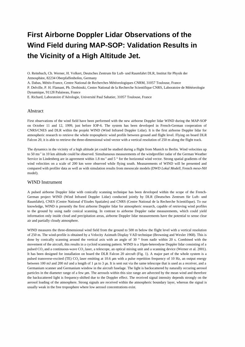
WIND measures the three-dimensional wind field from the ground to 500 m below the flight level with a vertical resolutionof 250 m. The wind-profile is obtained by a Velocity Azimuth Display VAD technique (Browning and Wexler 1968). This isdone by conically scanning around the vertical axis with an angle of 30 ° from nadir within 20 s. Combined with themovement of the aircraft, this results in a cycloid scanning pattern. WIND is a 10µm-heterodyne Doppler lidar consisting of apulsed CO2 and a continuous-wave CO2 laser, a telescope, an optical mixing unit and a scanning device (Werner et al. 2001).It has been designed for installation on board the DLR Falcon 20 aircraft (Fig. 1). A major part of the whole system is apulsed transverse-excited (TE) CO2 laser emitting at 10.6 µm with a pulse repetition frequency of 10 Hz, an output energybetween 100 mJ and 200 mJ and a length of 1 µs to 3 µs. It is sent out via the same telescope that is used as a receiver, and aGermanium scanner and Germanium window in the aircraft fuselage. The light is backscattered by naturally occuring aerosolparticles in the diameter range of a few µm. The aerosols within this size range are advected by the mean wind and thereforethe backscattered light is frequency-shifted due to the Doppler effect. The received signal intensity depends strongly on theaerosol loading of the atmosphere. Strong signals are received within the atmospheric boundary layer, whereas the signal isusually weak in the free troposphere where low aerosol concentrations exist.

WIND measurements during MAP-SOP

First observations of the wind field have been performed with WIND during the two flights on board the Falcon 20 aircrafton October 11 and 12, 1999, just before IOP-6. The scientific objective for a participation of WIND was to document flowsabove the Brenner pass and the atmospheric boundary layer organisation in the Italian Po valley. For the purpose ofvalidation, a flight around the windprofiler radar WPR of the German Weather Service at Lindenberg near Berlin wasconducted on 12 October 1999 (Reitebuch et al. 2001). The dynamics in the vicinity of a high altitude jet could be studiedduring this flight. The result of the validation is reported here, whereas the measurements over the Brenner Pass are presentedby elsewhere (Dabas et al. 2001).

The synoptic condition on October 12, 1999 is characterised by a low pressure region over the eastern baltic sea and a highover the British Islands. The winds over Southern Germany and the Alps were quite low, but strong windgradients weredominant towards the Northeast. The horizontal wind velocity over Europe retrieved from the Lokal Modell of the GermanWeather Service shows strong northwesterly winds with a maximum up to 60 ms-1 in the upper troposphere over NorthernGermany and Denmark. The investigated area around Lindenberg was just at the southern edge of a strong jet stream. Cirrusand cumulus clouds could be observed, during the flight above the area.

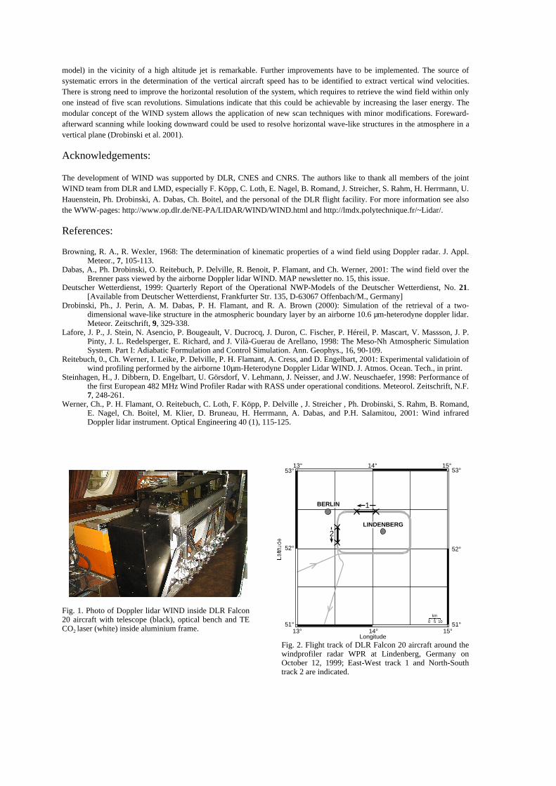
The flight track around the WPR is shown in Fig. 3. The Falcon was flying several rectangular boxes centered at Lindenberg,Germany (52.21N, 14.13E) in a height of 11.3 km. Comparisons of wind profiles taken during flights from East to West(flight track 1, 13:35 UTC) and North to South (flight track 2, 13:40 UTC) are made with the windprofiler radar WPR(Steinhagen et al. 1998) and the Lokal Modell LM of the German Weather Service (DWD 1999). Measurements of theWIND Doppler lidar were obtained by averaging data over five scanner revolutions (100 s), which corresponds to a width ofthe swath at ground of 13 km and an along-track resolution of 20 km. Measurements of the WPR are averaged over 25minutes. Data from LM were calculated for a time of 13:30 UTC with a prognostic run beginning at 12:00 UTC.

Results

A comparison of the profiles for the horizontal wind vector is shown in Fig. 4 for the East-West flight track 1. Profiles of thehorizontal wind velocity show a remarkable wind shear from 10 ms-1 near ground up to 50 ms-1 at 10 km height. Thecorrespondence among the measurements from WIND Doppler lidar, WPR and the 1.5-hour prediction of Lokal Modell LMis excellent, except in a region from 4 km to 6 km during flight track 1, where SNR was very low. A closer look at the height8 km to 10 km from profiles of flight track 1 and 2 shows a small decrease in wind velocity of 2 ms-1 for the WIND and LMdata. This is due to the horizontal wind gradient on a scale of 50 km and demonstrates the capabilitiy of WIND to resolvesmall changes of wind velocity. A statistical comparison has been performed although it is only limited to a small number ofdata on the two flight tracks. The comparison of the WIND and WPR measurements yield a standard deviation of 1.8 ms-1, abias of -0.7 ms-1 and a relative standard deviation of 6 %; the corresponding values for the WIND and LM comparison are astandard deviation of 1.5 ms-1, a bias of -0.5 ms-1 and a relative standard deviation of 6 %. The result of this comparison arequite remarkable, taking into account that the calculated values for standard deviation includes statistical errors from bothsources.

While flying south from Berlin to Munich strong spatial gradients of the horizontal wind speed could be observed. Fig. 4shows the WIND measurements, while flying from southwards for 250 km in the vicinity of the jet-stream beginning at theNorthern side of the rectangular box (Fig. 2). An overall of 11 wind vector profiles with a separation of 25 km were obtained,when averaging over 5 scanner revolutions. Mesoscale simulations from the non-hydrostatic model meso-NH (Lafore et al.1998) with a horizontal resolution of 10 km are compared to measurements of the WIND system for the same slice throughthe atmosphere (Fig. 5). Simulations are performed for 14:00 UTC, based on an initialisation on the 12:00 UTC analysis ofARPEGE or ECMWF. The agreement between the meso-NH and WIND measurements is good in all levels. A significantdifference could be observed for the higher wind speeds in the jet-level between the initialisation with ARPEGE andECMWF. The simulation output initialised with ARPEGE, which is slightly higher than ECMWF, corresponds better to theWIND measurements with a bias of 0.3 ms-1 and a standard deviation of 1.9 ms-1.

Conclusion

The first conical scanning Doppler lidar on airborne platform has been successfully developed in the scope of the French-German WIND project. First flights in 1999 did demonstrate the excellent capability for measuring the whole wind profilebetween ground and flight level with a nadir pointing conical scanning lidar. Comparisons with windprofiler radarmeasurements of the German Weather Service showed an correspondence within 1.5 ms-1 and 5 ° for the horizontal windvector. The agreement between WIND measurements and mesoscale models models (DWD Lokal Modell, French meso-NH

model) in the vicinity of a high altitude jet is remarkable. Further improvements have to be implemented. The source ofsystematic errors in the determination of the vertical aircraft speed has to be identified to extract vertical wind velocities.There is strong need to improve the horizontal resolution of the system, which requires to retrieve the wind field within onlyone instead of five scan revolutions. Simulations indicate that this could be achievable by increasing the laser energy. Themodular concept of the WIND system allows the application of new scan techniques with minor modifications. Foreward-afterward scanning while looking downward could be used to resolve horizontal wave-like structures in the atmosphere in avertical plane (Drobinski et al. 2001).

Acknowledgements:

The development of WIND was supported by DLR, CNES and CNRS. The authors like to thank all members of the jointWIND team from DLR and LMD, especially F. Köpp, C. Loth, E. Nagel, B. Romand, J. Streicher, S. Rahm, H. Herrmann, U.Hauenstein, Ph. Drobinski, A. Dabas, Ch. Boitel, and the personal of the DLR flight facility. For more information see alsothe WWW-pages: http://www.op.dlr.de/NE-PA/LIDAR/WIND/WIND.html and http://lmdx.polytechnique.fr/~Lidar/.

References:

Browning, R. A., R. Wexler, 1968: The determination of kinematic properties of a wind field using Doppler radar. J. Appl.Meteor., 7, 105-113.

Dabas, A., Ph. Drobinski, O. Reitebuch, P. Delville, R. Benoit, P. Flamant, and Ch. Werner, 2001: The wind field over theBrenner pass viewed by the airborne Doppler lidar WIND. MAP newsletter no. 15, this issue.

Deutscher Wetterdienst, 1999: Quarterly Report of the Operational NWP-Models of the Deutscher Wetterdienst, No. 21.[Available from Deutscher Wetterdienst, Frankfurter Str. 135, D-63067 Offenbach/M., Germany]

Drobinski, Ph., J. Perin, A. M. Dabas, P. H. Flamant, and R. A. Brown (2000): Simulation of the retrieval of a two-dimensional wave-like structure in the atmospheric boundary layer by an airborne 10.6 µm-heterodyne doppler lidar.Meteor. Zeitschrift, 9, 329-338.

Lafore, J. P., J. Stein, N. Asencio, P. Bougeault, V. Ducrocq, J. Duron, C. Fischer, P. Héreil, P. Mascart, V. Massson, J. P.Pinty, J. L. Redelsperger, E. Richard, and J. Vilà-Guerau de Arellano, 1998: The Meso-Nh Atmospheric SimulationSystem. Part I: Adiabatic Formulation and Control Simulation. Ann. Geophys., 16, 90-109.

Reitebuch, 0., Ch. Werner, I. Leike, P. Delville, P. H. Flamant, A. Cress, and D. Engelbart, 2001: Experimental validatioin ofwind profiling performed by the airborne 10µm-Heterodyne Doppler Lidar WIND. J. Atmos. Ocean. Tech., in print.

Steinhagen, H., J. Dibbern, D. Engelbart, U. Görsdorf, V. Lehmann, J. Neisser, and J.W. Neuschaefer, 1998: Performance ofthe first European 482 MHz Wind Profiler Radar with RASS under operational conditions. Meteorol. Zeitschrift, N.F.7, 248-261.

Werner, Ch., P. H. Flamant, O. Reitebuch, C. Loth, F. Köpp, P. Delville , J. Streicher , Ph. Drobinski, S. Rahm, B. Romand,E. Nagel, Ch. Boitel, M. Klier, D. Bruneau, H. Herrmann, A. Dabas, and P.H. Salamitou, 2001: Wind infraredDoppler lidar instrument. Optical Engineering 40 (1), 115-125.

Fig. 1. Photo of Doppler lidar WIND inside DLR Falcon20 aircraft with telescope (black), optical bench and TECO2 laser (white) inside aluminium frame.

Fig. 2. Flight track of DLR Falcon 20 aircraft around thewindprofiler radar WPR at Lindenberg, Germany onOctober 12, 1999; East-West track 1 and North-Southtrack 2 are indicated.

52°

51°13° 14° 15°

53°

52°

51°

53°13° 14° 15°

BERLIN

LINDENBERG

Longitude

km

0 5 10

1

2

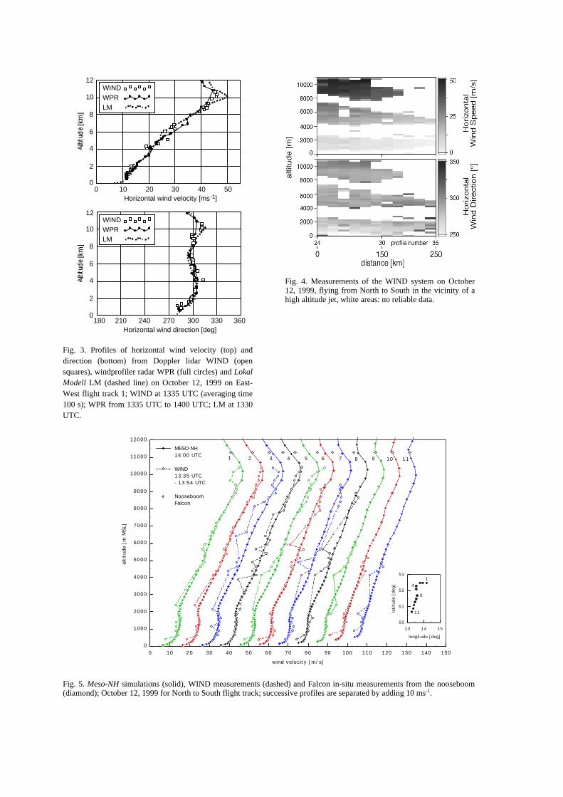
Fig. 3. Profiles of horizontal wind velocity (top) anddirection (bottom) from Doppler lidar WIND (opensquares), windprofiler radar WPR (full circles) and LokalModell LM (dashed line) on October 12, 1999 on East-West flight track 1; WIND at 1335 UTC (averaging time100 s); WPR from 1335 UTC to 1400 UTC; LM at 1330UTC.

Fig. 4. Measurements of the WIND system on October12, 1999, flying from North to South in the vicinity of ahigh altitude jet, white areas: no reliable data.

Fig. 5. Meso-NH simulations (solid), WIND measurements (dashed) and Falcon in-situ measurements from the nooseboom(diamond); October 12, 1999 for North to South flight track; successive profiles are separated by adding 10 ms-1.

WINDWPRLM

12

0

2

4

6

8

10

0 10 20 30 40 50Horizontal wind velocity [ms-1]

210 240 270 300 330Horizontal wind direction [deg]

360

WINDWPRLM

12

0

2

4

6

8

10

180

0 10 20 30 40 50 60 70 80 90 100 110 120 130 140 150

wind velocity [m/s]

0

1000

2000

3000

4000

5000

6000

7000

8000

9000

10000

11000

12000

alti

tude

[m

MSL

]

MESO-NH14:00 UTC

WIND13:35 UTC - 13:54 UTC

NooseboomFalcon

13 14 15

longitude [deg]

50

51

52

53

lati

tude

[de

g]

1

4

6

11

1 2 3 4 5 6 7 8 9 10 11