Firm and Worker Dynamics in a Frictional Labor Market

Firm and Worker Dynamics in a Frictional Labor Market *

Adrien Bilal†, Niklas Engbom‡, Simon Mongey§, and Giovanni L. Violante¶

September 16, 2021

Abstract

This paper integrates the classic theory of firm boundaries, through span of control or taste for variety,

into a model of the labor market with random matching and on-the-job search. Firms choose when to

enter and exit, whether to create vacancies or destroy jobs in response to shocks, and Bertrand-compete

to hire and retain workers. Tractability is obtained by proving that, under a parsimonious set of assump-

tions, all worker and firm decisions are characterized by their joint surplus, which in turn only depends

on firm productivity and size. The job ladder in marginal surplus that emerges in equilibrium deter-

mines net poaching patterns by firm characteristics that are in line with the data. As frictions vanish, the

model converges to a standard competitive model of firm dynamics. The combination of firm dynamics

and search frictions allows to: (i) quantify the misallocation cost of frictions; (ii) replicate elusive life-

cycle growth profiles of superstar firms; and (iii) make sense of the failure of the job ladder around the

Great Recession as a result of the collapse of firm entry.

Keywords: Diminishing Returns to Scale, Firm Dynamics, Great Recession, Job Turnover, Marginal

Surplus, Misallocation, Net Poaching, On the Job Search, Search, Frictions, Unemployment, Vacancies,

Worker Flows.

JEL Classification: D22, E23, E24, E32, J23, J63, J64, J69.

*The view included are those of the authors and do not represent those of the Federal Reserve System.

†Harvard University and NBER‡New York University, CEPR and NBER§Federal Reserve Bank of Minneapolis, University of Chicago and NBER¶Princeton University, CEBI, CEPR, IFS, IZA, and NBER

1 Introduction

Aggregate production in the economy is divided into millions of firms, each facing idiosyncratic fluc-

tuations in its productivity and demand. Understanding the process of labor reallocation across these

production units is important for several reasons. In the long run, reallocating labor away from unpro-

ductive firms toward more productive firms enhances aggregate productivity and growth. In the short

run, the propagation of sectoral and aggregate shocks depends on how quickly labor flows across firms

and between unemployment and employment. From a normative perspective, understanding the po-

tential welfare losses or gains due to reallocation is necessary for assessing the efficacy of policies that

subsidize jobless workers, protect employment, or advantage particular sectors or firms.

The labor reallocation process has three key properties. First, it has distinct layers: the entry and exit

of firms, the creation and destruction of jobs at existing firms, and the turnover of workers across existing

jobs. Second, it is intermediated by labor markets that are frictional, as revealed by the coexistence

of vacancies and job seekers. Third, around half of worker turnover occurs through direct job-to-job

transitions: most new hires come from another firm rather than from unemployment.

Therefore, addressing labor reallocation requires a framework with two central elements. First, a

theory of the firm (i.e., its boundaries) and of firm dynamics (entry, growth, separations, exit). Second,

a theory of worker flows intermediated by frictional labor markets that allows for on-the-job search

and job-to-job mobility (i.e., poaching). Quantitatively, such a framework should account for a new

body of time series and cross-sectional evidence—emerging from matched employer-employee data—

that describes the relationship between firm characteristics and the direction and composition of worker

flows.1

This paper presents a new model with these features. A firm is a profit maximizing owner of a tech-

nology with decreasing returns to scale and stochastic productivity, that chooses optimally whether to

enter and when to exit the market.2 Firms grow by posting costly vacancies that are randomly matched

to either unemployed or employed workers. Worker flows occur when matched workers determine that

the value of working at the newly matched firm exceeds their value of unemployment or employment in

their current firm. In general, with decreasing returns to scale in production, these values are a compli-

cated function of a high dimensional state vector that includes distributions of wages or worker values

inside the firm. This makes the problem seem intractable.

1If we consider hires for a particular firm type (e.g., young, small and fast-growing), by composition we mean the splitbetween hires from unemployment and those from employment. Within hires from employment, direction refers to the charac-teristics of the employers between which workers are reallocated.

2Or, equivalently, a monopolistic producer facing a downward sloping demand curve with a stochastic shifter. These twointerpretations are isomorphic in our model.

1

Our first contribution is to set out a parsimonious set of assumptions that are sufficient for tractabil-

ity. Our assumptions place a minimal structure on the contractual environment such that the state vec-

tor becomes manageable. Three assumptions on bargaining and surplus sharing are common to many

single-worker firm environments: (i) lack of commitment; (ii) wage contract renegotiation by mutual

consent; (iii) Bertrand competition among employers for employed jobseekers. Two further assump-

tions are required in our new multi-worker firm environment: (iv) no value is lost in internal wage

renegotiations between a firm and its incumbent workers; and (v) vacancy policies maximize combined

firm and worker value—for which we offer an explicit microfoundation. Under these assumptions, firm

and workers’ decisions are privately efficient, as if the firm and incumbent workers maximize their total

value. The state variables of the total value function are only two: firm size (n) and productivity (z).

Two other ingredients are vital to achieve tractability. First, we work in continuous time. In a small

interval of time only one random event may occur. For example, a firm only needs to deal with one of

its employee meeting another firm, not all combinations of its employees meeting other firms. Second,

we take the continuous limit of a discrete workforce. Worker flows are determined by comparing the

change in total value that would arise if a worker joins or leaves a firm. With a continuous measure of

workers, this marginal value can be conveniently expressed as a partial derivative of total value.

We show that total and marginal value are sufficient for characterizing firm and worker dynamics.

Marginal value pins down hiring: facing a convex vacancy cost, firms post vacancies until the marginal

cost of a vacancy is equal to the expected marginal value of hiring.3 Marginal value also pins down

separations: facing a decreasing marginal product of labor, firms fire workers until the marginal value

of a worker equals the value of unemployment. When total value is less (more) than the firm owner’s

outside option, the firm exits (enters). Finally, in equilibrium, marginal values determine the direction

of worker flows. Workers climb a job ladder in marginal value, quitting when on-the-job search delivers

a match with a higher marginal value firm. An intuitive Bellman equation accounts for the evolution of

the total value, while a law of motion reflecting frictional labor reallocation accounts for the evolution of

the firm size and productivity distribution.4

Our second contribution exploits the mathematical tractability of our framework to analytically char-

acterize equilibrium firm and worker reallocation. First, we analyze firm dynamics and job turnover

graphically in (n, z)-space by describing the regions in which a firm exits, fires and hires. Firms that exit

3Convex adjustment costs are among the solutions proposed by Elsby, Michaels, and Ratner (2019) to obtain empiricallyplausible sluggish adjustment of labor market aggregates, which is difficult to generate in models with fixed or linear costs.

4This representation uniquely pins down firm and worker dynamics, the subject of this paper, but is consistent with mul-tiple wage determination mechanisms that determine how this joint value is split. Wages, therefore, are not allocative in thatthe distribution of firms and flows of workers across firms is independent of wage dynamics. In order to study the model’simplication for wage dynamics, one has to make additional assumptions. We return on this point in Section 2.

2

and fire always destroy jobs. Hiring firms may either grow on net (creating jobs) or shrink on net (de-

stroying jobs) because some of their workers quit to firms with a higher rank on the marginal value lad-

der. Second, we decompose sources of net employment growth for hiring firms into the different types

of gross flows: hires and separation from/to unemployment and from/to employment via poaching.

This decomposition varies systematically with the firm states (n, z) that determine marginal surplus.

Third, we establish that our framework generalizes existing work by studying the limiting behaviors

of our economy. As decreasing returns to scale vanish, the economy converges to one in which single-

worker firms operate in a frictional labor market à la Postel-Vinay and Robin (2002). As frictions vanish,

the economy converges to one in which multi-worker firms operate in a competitive labor market à la

Hopenhayn (1992). Surprisingly, on the job search is necessary for this result, as it provides the mecha-

nism that equates the marginal products of labor across firms in the limit. As in Hopenhayn (1992), the

limit features a non-degenerate firm size distribution. This is in sharp contrast to the frictionless limit of

an economy with constant returns which would see one firm hire all workers in the economy.

Our third contribution exploits the computational tractability of our framework to quantitatively

analyze equilibrium firm and worker reallocation. We estimate the model by Simulated Method of Mo-

ments, targeting cross-sectional moments of the size distribution of firms, firm dynamics, job flows and

worker flows for the U.S. economy. We argue that parameters are well-identified.

As a test of the model, we show that our theory is quantitatively consistent with new facts from US

employer-employee match data (Haltiwanger, Hyatt, Kahn, and McEntarfer, 2018). In the data, job-to-

job flows vary systematically across firms: young firms poach workers from older firms, but firm size

is only weakly correlated with net poaching. In our model, with decreasing returns, a small, young,

high productivity firm that is yet to grow, has a high marginal value of a worker which places it near

the top of the job ladder. Meanwhile, older firms that are small have reached that size because of low

productivity, which places them at the opposite end of the ladder. Both are small, but the young firms’

vacancies are more likely to attract workers from competitors. To guide future measurement we show

that average labor productivity and firm growth are observables that are strongly positively correlated

with marginal surplus, so predictive of net poaching and job ladder rank.

We then consider three applications of our model in which we highlight the misallocation effects of

labor market frictions along three dimensions of the data: cross-section, firm life-cycle, and time-series.

First, we show that an increase in match efficiency that drives unemployment close to zero also

accelerates worker reallocation to more productive firms, and in doing so reduces the cross-sectional

misallocation of labor across firms and raises TFP by nearly 5 percent.

In our second application, we argue that allowing for misallocation via labor market frictions over-

3

comes a shortcoming of competitive firm dynamics models first identified by Luttmer (2011). In these

environments, jointly matching the volatility of firm growth and the size of young firms requires, respec-

tively, small shocks and very low productivity of entrants. Consequently, firms take several hundreds of

years to reach the tail of the size distribution, in contrast to the data where this transition is much faster.

In our environment, labor market frictions impede to reach the optimal size instantaneously and allow

a distribution of young firms that are all small in size, but in which some have very high productivity.

With decreasing returns and on the job search these firms are at the very top of the job ladder, and move

quickly toward the tail of the size distribution.

Third, our model offers an intuitive interpretation for firm and worker dynamics around the Great

Recession, and links them to the observed decline in TFP through a rise in labor misallocation. The re-

cession featured a sharp drop in firm entry and a decline in job-to-job reallocation of workers, which

has been characterized as a ‘failure of the job ladder’ (Siemer, 2014; Moscarini and Postel-Vinay, 2016).

Theoretically, our model offers a unifying explanation. A transitory shock to the discount rate, which is

a commonly used stand-in for worsening financial frictions (Hall, 2017), lowers the value of entry and

shrinks the population of young, high marginal surplus firms with high equilibrium net poaching rates.

Vacancy posting collapses among these firms and labor reallocation up the ladder breaks down. Quan-

titatively, the shock generates the empirical contractions in aggregate employment, job-to-job mobility,

firm entry, vacancies and output. In the cross-section, the model matches the decline in net poaching at

high productivity firms, and increase in net poaching at low productivity firms (Haltiwanger, McEntar-

fer, and Staiger, 2021). The resulting misallocation of labor causes a slump in total factor productivity

that accounts for a quarter of the large decline in output.

Collectively, these applications demonstrate that our new theoretical framework is a useful platform

to jointly analyze the microeconomic dynamics of firms and workers in a frictional labor market, and

how these shape macroeconomic outcomes.

Literature

Our paper connects two literatures that share an idea going back to Lucas (1978): the dominant force that

delivers a non-degenerate firm-size distribution is the combination of diminishing returns in production

and heterogeneity in productivity.

The first literature studies equilibrium models of single-product firm dynamics with competitive

labor markets. Classic examples are Hopenhayn (1992), Hopenhayn and Rogerson (1993), and Luttmer

4

(2011).5 Recent examples, with applications to the Great Recession, are Arellano, Bai, and Kehoe (2019),

Clementi and Palazzo (2010) and Sedlácek (2020). Like these models, our framework features entry, exit,

and non degenerate distributions of firm size and age. Unlike these models, the employment adjustment

costs that firms face are endogenous. They depend on the firm’s likelihood of poaching workers from

competitors and the expected transfers this requires. Both are a function of the firm rank on the marginal

surplus ladder, which is an equilibrium object.

The second literature comprises a number of papers that model multi-worker firms in frictional labor

markets. Here, two approaches have been taken: directed search and random search.

Under the directed search approach, Kaas and Kircher (2015) and Schaal (2017) generate firm em-

ployment dynamics resembling those in the micro data.6 Building on Menzio and Shi (2011), Schaal

(2017) allows for on the job search, and thus is the closest counterpart to our framework. A drawback

of directed search is that the probability that a firm hires from a competitor versus from unemployment

is not determined.7 As a result, this class of models cannot speak to the systematic variation across firm

types in net poaching rates or the composition of hires. A model consistent with these facts is one of the

objectives of our analysis.

Under the random search approach, Elsby and Michaels (2013) and Acemoglu and Hawkins (2014)

solve models where firms face decreasing returns in production, stochastic productivity, linear vacancy

costs, and wages determined by Nash bargaining.8 Both generate employment relationships with a large

average surplus and small marginal surplus. Elsby and Michaels (2013) demonstrate that the latter yields

a volatile job-finding rate over the cycle, while the former avoids a high separation rate. This resolves

the tension identified by Shimer (2005) in the Diamond-Mortensen-Pissarides framework. Gavazza,

Mongey, and Violante (2018) introduce recruiting intensity and financial constraints to account for the

sharp drop in aggregate match efficiency around the Great Recession. All of these models abstract from

search on the job.9

Random search models with wage posting feature both on-the-job search and a firm-size distribution.

5For a review of the literature see also Luttmer (2010).6It is worth remarking that these two papers had very different objectives to ours. Kaas and Kircher (2015) illustrate that a

key advantage of directed search, the efficiency and block-recursivity properties of equilibrium, extends to models with ‘large’firms. Schaal (2017) proves this property is also robust to the addition of on-the-job-search and studies aggregate uncertaintyshocks in the context of the Great Recession.

7In the equilibrium of directed search models, net hiring costs are equated across firms through free entry, which impliesthat firms are indifferent across the markets in which they search for workers. The probability that a separation from a firm isto employment or unemployment, however, is determined.

8Bertola and Caballero (1994) derive closed form results under a linear approximation to both marginal product and convexvacancy costs, and a two state Markov process for productivity.

9Fujita and Nakajima (2016) introduce on-the-job search and study the dynamics of job-job flows over the business cycle.However, solving their equilibrium requires worker’s outside option to always equal value of unemployment. Hence workersare always indifferent between searching/working and staying/moving.

5

Bilal and Lhuillier (2021) introduce decreasing returns in the steady-state Burdett and Mortensen (1998)

environment, but handling productivity shocks remains out of reach. With constant returns to scale,

out of steady-state dynamics in the Burdett and Mortensen (1998) model are studied by Moscarini and

Postel-Vinay (2013, 2016), Coles and Mortensen (2016), Engbom (2017), Gouin-Bonenfant (2018) and

Audoly (2019). In these models the size distribution is non degenerate only because of the existence

of search frictions: as frictions disappear, all workers become employed at the most productive firm.

Instead, as explained, the frictionless limit of our model is a version of Hopenhayn (1992). Another

implication of such environments is that large firms, which pay higher wages in the model, should

systematically poach from small firms, while the data suggest otherwise.

Within the random search literature, we build on the set-up developed by Postel-Vinay and Robin

(2002): Bertrand competition between employers for workers and wage renegotiation under mutual

consent. This environment has become another workhorse of the literature due to its tractability and

empirically plausible wage dynamics.10 As opposed to the Postel-Vinay and Robin (2002) framework,

the probability of filling a vacancy in our model is not a function of the exogenous distribution of firms’

productivity, but a function of the endogenous distribution of firms’ marginal surpluses, which itself de-

pends on how the equilibrium of the frictional labor market allocates workers across heterogeneous

firms. Kiyotaki and Lagos (2007) develop a version that is a step closer to us. Their firms have a capacity

of one position—an extreme version of decreasing returns— and when an occupied firm meets another

worker, it engages in renegotiation with its incumbent worker. Our contribution is to generalize this

sequential auction protocol to multi-worker firms, show how one can still solve the model’s equilibrium

through the notion of joint surplus, and do so in a tractable way.

The final expression for joint surplus that features among our equilibrium conditions is reminiscent

of that in Lentz and Mortensen (2012): a version of Klette and Kortum (2004) with on-the-job search in

which a firm’s demand for labor is limited by demand for its portfolio of products. While they assume

that all decisions are based on joint firm-workers values, we derive this result from primitives, provide

a characterization of the equilibrium and illustrate how to use the model for a quantitative analysis of

newly documented empirical patterns. Our central finding that a job ladder in marginal surplus arises

in equilibrium is closely related to contemporaneous work by Elsby and Gottfries (2021) who elegantly

characterize a special case of our environment with linear vacancy costs and no endogenous entry and

exit. In their setting, firm value and policies are a function of a single state variable, the marginal product

of labor. In our theory, marginal surplus is related to the current and future marginal products of labor,

10Recent examples are Postel-Vinay and Turon (2010); Jarosch (2021); Lindenlaub and Postel-Vinay (2016); Borovicková(2016); Lise and Robin (2017).

6

and also depends on average surplus through the exit decision. Nevertheless, in our calibrated model,

the correlation between marginal surplus and the current marginal product of labor is high. Finally, the

endogenous entry decision, not in Elsby and Gottfries (2021), is at the heart of three main applications of

our model.

Outline. Section 2 establishes the physical and contractual environment. Section 3 states our joint value

representation and its key properties. Section 4 defines an equilibrium and characterizes firm dynamics

and worker flows. Section 5 estimates the model on US data and discusses the model’s fit. Section 6 uses

the estimated model to examine, under different angles, how search frictions impede reallocation of labor

across firms. Section 7 concludes. The Appendix contains all proofs and a discussion of identification.

2 Model

2.1 Physical environment

Time is continuous and there is no aggregate uncertainty. There are two types of agents. An exogenous

mass n of ex-ante identical, infinitely-lived workers that are risk neutral, discount the future at rate ρ and

are endowed with one unit of time each period which is inelastically supplied to production. An infinite

mass of homogeneous potential firms, of which an endogenous mass become operating firms.

Production technology. There is a single homogeneous good. Workers may either be employed or

unemployed. Unemployed workers produce b units of the final good. A firm with productivity z ∈ Z

employing n workers produces y(z, n) units of the final good, where y(z, n) is strictly increasing in z and

n and concave in n, i.e. ynn(z, n) ≤ 0.11,

Firm demographics. A potential firm becomes an operating firm by paying a fixed cost c0. This cost

entitles the firm to a draw of productivity z from the distribution Π0 (z) and to n0 workers, taken from

unemployment. After entry, z evolves stochastically. At any point in time a firm may exit, at which point

all of its workers become unemployed and the firm produces ϑ > 0 units of the final good which we

refer to as its scrap value. Denote the mass of entrants m0 and the mass of operating firms m.

Matching technology. Hiring firms and job-seekers meet in a frictional labor market. The total number

of meetings is given by the CRS aggregate matching technology m(s, v). Inputs to this function are total

11In addition, we assume that for any z the Inada conditions hold with respect to n: (i) y(z, 0) = 0, (ii) limn→0 yn(z, n) = +∞,and (iii) limn→+∞ yn(z, n) = 0.

7

vacancies v and total units of search efficiency s = u+ ξ(n− u), where the parameter ξ determines the

relative search efficiency of employed workers (labor force minus the unemployed). Search is random

in the following sense. A firm pays a cost c(v; z, n) to post v vacancies, where c is increasing and convex

in v. Each vacancy is matched with a worker at rate q(s, v) = m(s, v)/v. The worker is unemployed

with probability φ = (u/s) , and employed with probability (1− φ). A worker faces no cost of search.

An unemployed worker meets a firm at rate λU(s, v) = m(s, v)/s. An employed worker meets a firm

at rate λE(s, v) = ξλU(s, v). The rates q and λU can be expressed in terms of market tightness θ = (v/s).

If constituted, the match of a worker to a firm exogenously expires at rate δ, and the worker becomes

unemployed.

States. Let x be the vector of state-variables for the firm. This vector includes all individual state vari-

ables of all workers at the firm. For now, we do not specify exactly what is in x and, along the way, define

a number of functions that map x at instant t into a new state vector at t + dt. Let H (x) be the measure

of x across firms in the economy, v(x) the number of vacancies created by a firm with state x, and n(x)

employment at firm x. The total mass of vacancies and employed workers in the economy are

v =

v (x) dH (x) , n = n− u =

n (x) dH (x) .

Densities that appear in agents’ problems describe vacancy- and employment-weighted distributions:

hv (x) =v(x)h(x)

v, hn (x) =

n(x)h(x)n

.

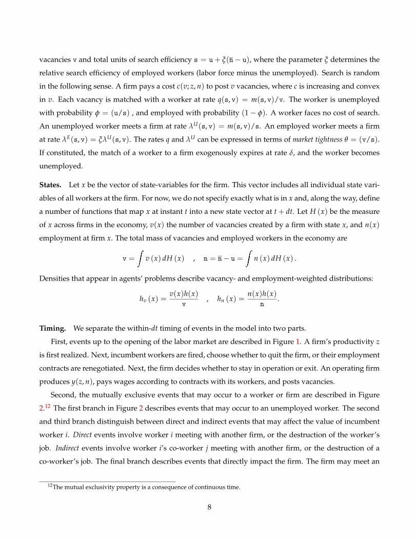
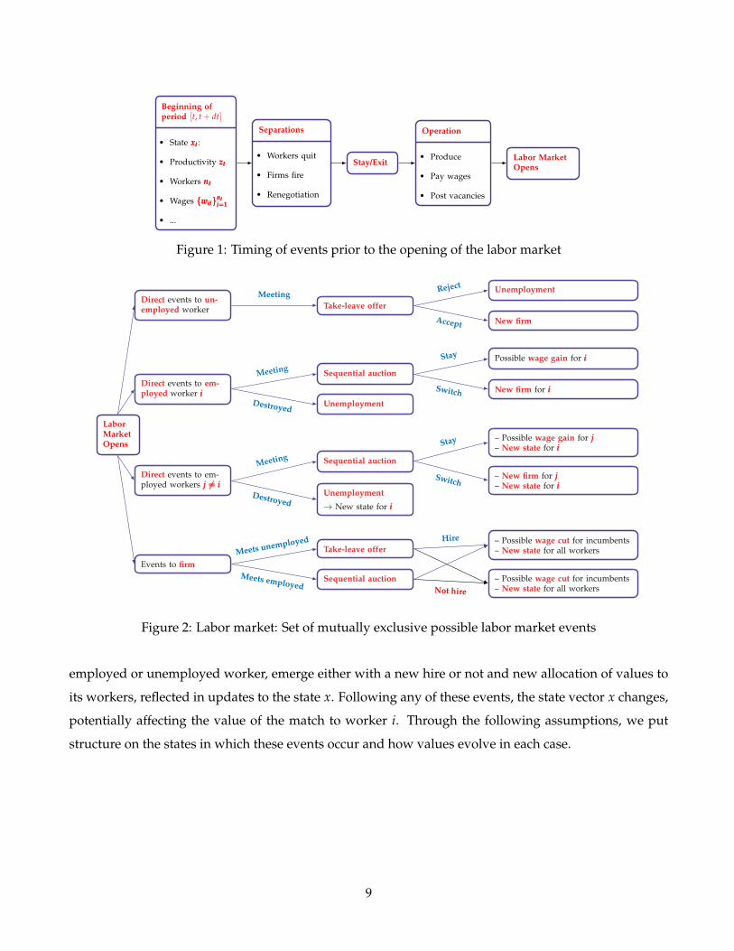
Timing. We separate the within-dt timing of events in the model into two parts.

First, events up to the opening of the labor market are described in Figure 1. A firm’s productivity z

is first realized. Next, incumbent workers are fired, choose whether to quit the firm, or their employment

contracts are renegotiated. Next, the firm decides whether to stay in operation or exit. An operating firm

produces y(z, n), pays wages according to contracts with its workers, and posts vacancies.

Second, the mutually exclusive events that may occur to a worker or firm are described in Figure

2.12 The first branch in Figure 2 describes events that may occur to an unemployed worker. The second

and third branch distinguish between direct and indirect events that may affect the value of incumbent

worker i. Direct events involve worker i meeting with another firm, or the destruction of the worker’s

job. Indirect events involve worker i’s co-worker j meeting with another firm, or the destruction of a

co-worker’s job. The final branch describes events that directly impact the firm. The firm may meet an

12The mutual exclusivity property is a consequence of continuous time.

8

Beginning ofperiod [t, t + dt]

• State xtxtxt:

• Productivity ztztzt

• Workers ntntnt

• Wages witnti=1witnti=1witnti=1

• ...

Separations

• Workers quit

• Firms fire

• Renegotiation

Stay/Exit

Operation

• Produce

• Pay wages

• Post vacancies

Labor MarketOpens

Figure 1: Timing of events prior to the opening of the labor market

LaborMarketOpens

Direct events to un-employed worker Take-leave offer

Meeting UnemploymentReject

New firmAccept

Direct events to un-employed worker Take-leave offer

Meeting UnemploymentReject

New firmAccept

Direct events to em-ployed worker iii

Sequential auctionMeeting

UnemploymentDestroyed

Possible wage gain for iiiStay

New firm for iiiSwitchDirect events to em-ployed worker iii

Sequential auction

UnemploymentDestroyed

Possible wage gain for iiiStay

New firm for iiiSwitch

Direct events to em-ployed workers j 6= ij 6= ij 6= i

Sequential auctionMeeting

Unemployment

→ New state for iiiDestroyed

– Possible wage gain for jjj– New state for iiiStay

– New firm for jjj– New state for iii

SwitchDirect events to em-ployed workers j 6= ij 6= ij 6= i

Sequential auction

Unemployment

→ New state for iiiDestroyed

– Possible wage gain for jjj– New state for iiiStay

– New firm for jjj– New state for iii

Switch

Events to firm

Take-leave offerMeets unemployed

Sequential auctionMeets employed

– Possible wage cut for incumbents– New state for all workers


Hire

Not hire

Events to firm

Take-leave offerMeets unemployed

Sequential auctionMeets employed



Hire

Not hire

Figure 2: Labor market: Set of mutually exclusive possible labor market events

employed or unemployed worker, emerge either with a new hire or not and new allocation of values to

its workers, reflected in updates to the state x. Following any of these events, the state vector x changes,

potentially affecting the value of the match to worker i. Through the following assumptions, we put

structure on the states in which these events occur and how values evolve in each case.

9

2.2 Information and contractual environment

The information structure is such that everything that is payoff relevant is observable by both firms and

workers, and thus we rule out private information by assumption.13 The contractual environment is

rooted in incomplete contract theory, where there is a key distinction between the information available

to firm and workers, and what is verifiable by a third party, e.g. a court, and hence contractible. The

only verifiable and hence contractible objects are the wage, whether the firm made the wage payment,

and whether the worker provided labor services. Therefore, a contract between the firm and one of its

workers is a binding agreement that specifies a constant wage, i.e. a fixed payment from the firm to the

worker, in exchange for labor services. This contract satisfies five assumptions:

(A-LC) Limited commitment. All parties are subject to limited commitment. In particular,

(a) Layoffs - Firms can fire workers at will.

(b) Quits - Workers can always quit into unemployment or to another firm when they meet one.

(c) Collective agreements - Workers cannot commit to any other worker inside the firm. De facto

this assumption rules out transfers among workers.

(A-MC) Mutual consent. The wage (contract) can be renegotiated only by mutual consent, i.e. only if one

party can credibly threaten to dissolve the match (the firm by firing, the worker by quitting). A

threat is credible when one of the two parties has an outside option that provides her with a value

that is higher than the value under the current contract.

(A-EN) External negotiation. An external negotiation is a situation where, through search, the firm comes

into contact with an external job seeker or an incumbent worker comes into contact with another

firm. In external negotiations, all offers are take-it-or-leave-it.

• In a meeting with an unemployed worker, the firm makes a take-leave offer to the worker.

• In a meeting with an employed worker, the two firms Bertrand compete through a sequential

auction. First, the poaching firm makes the take-leave wage offer. Second, the target firm

makes a take-leave counteroffer to the worker. Third, the worker decides.

(A-IN) Internal negotiation. An internal negotiation is any other situation where contracts between firm

and any incumbent workers are modified (following (A-MC), an internal negotiation takes place

13For example, the number of vacancies posted by the firm is observable to workers, and whether a particular incumbentworker has an outside offer (as well as the identity of the competing firm) is observable to the current firm and other incumbentworkers. See Lentz (2015) for an environment where on-the-job search behavior, including the identity of firms in outsidemeetings, is unobservable to the firm and cannot be directly contracted upon.

10

when any party has a credible threat). The only parties involved in an internal negotiation are those

that have a threat and those that are under that threat. We assume that—with respect to worker

and firm values—the internal negotiation is a zero-sum game and that participation is individually

rational for all parties.14 Apart from these assumptions we leave internal negotiation unrestricted.

(A-VP) Vacancy posting. The firm posts the privately efficient amount of vacancies, which is the one that

maximizes the sum of the values of the firm and its workers. Below we propose one possible

micro-foundation for (A-VP).

Discussion of assumptions. Assumption (A-LC) implies an environment with at-will employment.

(A-MC) is common under incomplete contracts and in the terminology of MacLeod and Malcomson

(1989) yields self-enforcing contracts, a feature consistent with most legal frameworks. (A-EN) is a par-

ticular protocol to resolve the game between two firms competing for a worker. Combined, these three

assumptions amount to the contractual environment of Postel-Vinay and Robin (2002). The authors

show that they lead to a joint value representation in the one-worker-one-firm model. We now discuss

how (A-IN) and (A-VP) are sufficient to extend this convenient representation to an environment with

multi-worker firms and diminishing marginal product of labor.

(A-IN) is a standard assumption in virtually all bargaining protocols. As such, it allows for a large

class of possible micro-foundations for the internal renegotiation game. Each would imply different

wage dynamics. The central takeaway is that, no matter the details of such a game and the ensuing

wages, if (A-IN) is satisfied then allocations are uniquely determined by joint value dynamics. This paper

focuses on allocations, i.e. firm and worker dynamics. We leave for future research an investigation of

what different internal renegotiation games imply for wage dynamics at the firm and worker level, and

which is most consistent with data on wages.

(A-VP) is admittedly a strong assumption, but necessary to simplify the environment for analytical

characterization and quantitative analysis. Absent (A-VP), the firm would over-post vacancies relative

to the privately efficient amount. The incentive to over-post comes from credible threats to layoff in-

cumbents and hence lower their wages. First, over-hiring threatens layoffs by lowering the marginal

product of labor, as extensively discussed by Stole and Zwiebel (1996) and Brügemann, Gautier, and

Menzio (2018). Second, if a posted vacancy matches with a job seeker with a low outside option, the

firm may have no intention of hiring but the match nonetheless generates a threat to swap the incumbent

14We adopt the standard definition of a zero-sum game: each individual’s gain or loss is exactly offset by losses and gains ofother participants. We also adopt the standard definition of individual rationality: after internal negotiation each player whoremains employed at the firm receives at least the outside option that was present before internal negotiation.

11

worker. Proceeding under either would require the full distribution of wages as a state variable, ruling

out tractability. Assumption (A-VP) resolves these issues.15

The presence of these inefficiencies and the need for an assumption like (A-VP) is unique to an envi-

ronment with DRS, on-the-job search and endogenous vacancy posting. With DRS and on-the-job-search,

but exogenous contact rates (as in Kiyotaki and Lagos, 2007), there is no endogenous vacancy choice and

these inefficiencies do not arise. With on-the-job search and constant returns, over-hiring does not occur

due to a constant marginal product of labor (Postel-Vinay and Robin, 2002), and hiring a worker that

matches with a vacancy is always profitable leaving the swap threat hollow. Without on-the-job search

but with decreasing returns, incumbents are all hired from unemployment and with the same outside

option are paid the same wage (Elsby and Michaels, 2013; Acemoglu and Hawkins, 2014). Over-hiring

occurs, but with a degenerate distribution of wages within the firm this does not impede tractability, and

swapping is not a threat because the job seeker and incumbent are paid the same wage. If not addressed,

both inefficiencies would render the model intractable.

We propose one possible micro-foundation for assumption (A-VP). The idea is to ex-ante remove

any gains to the firm from expected future wage cuts that would otherwise encourage excess vacancy

posting. We assume that workers anticipate that firm’s behavior and offer a preemptive wage cut that

leaves the firm indifferent between the efficient vacancy policy and the firm’s privately optimal policy.16

(A-VPI) After the firm announces its proposed vacancies for dt, a randomly selected incumbent worker

has the opportunity to make a take-leave counter-offer to the firm. The counter-offer specifies

acceptable wages for incumbents in exchange for an alternative spot vacancy policy.17

We conclude by noting that that in directed search environments, full state-contingent contracts and

one-sided commitment by firms deliver bilateral efficiency between a one-worker-one-firm pair (Menzio

and Shi, 2011), and private efficiency between a firm and its many workers (Schaal, 2017). We extend this

literature by showing that a similar joint value representation can also be achieved in an environment

with random search, incomplete contracts, and no commitment.

15In a different environment Hawkins (2015) allows full commitment to a fixed wage. This assumes away wage cuts, andhence delivers efficient vacancy posting.

16Alternative implementations could be based on the introduction of ‘social norms’ that prevent firms from cutting thewage of a worker and swapping an incumbent worker with a new worker. Because they would involve deviations from lackof commitment (A-LC), we do not emphasize these alternative implementations in this paper.

17This assumption does not require commitment because it is not state-contingent. It is a ‘spot contract’ between the partiesinvolved: a transfer in exchange for an immediate action.

12

3 Joint value representation

Having described the economy’s environment and the contract space, we now describe the main the-

oretical result of the paper. For presentation purposes, the environment is specialized in two ways.

First, each firm employs a continuum of workers n. Second, productivity follows a diffusion dzt =

µ(zt)dt + σ(zt)dWt.18

Result. All allocative decisions in the economy—entry, exit, vacancy posting and mobility of workers

between firms—are determined by the joint value, Ω(z, n). The joint value equals the present discounted

value of an operating firm’s profits plus the present discounted value of lifetime utility of its incumbent

workers, and satisfies the following, where U is lifetime utility of an unemployed worker:

ρΩ (z, n) = maxv≥0

y (z, n)− c (v; z, n) (1)

EU job destruction: + δn[U −Ωn

(z, n)]

UE unemployed hire: + φq(θ)v[Ωn(z, n)−U

]EE poaching hire: + (1− φ)q(θ)v

max

Ωn(z, n)−Ωn

(z′, n′

), 0

dHn(z′, n′

)Shock: + µ(z)Ωz

(z, n)+

σ(z)2

2Ωzz

(z, n).

Firms’ operation requires (z, n) to be interior to an exit boundary, and an additional layoff boundary deter-

mines when separations occur:

Exit boundary: Ω(z, n) ≥ ϑ + nU, , Layoff boundary: Ωn(z, n) ≥ U. (2)

Conditions (1) and (2) represent the solution of the Hamilton-Jacobi-Bellman variational inequality,

which we include for completeness in Appendix B, equation (22), along with a discussion on the deriva-

tion of the boundary conditions. The entry decision can be written in terms of joint value as:

Entry condition:

Ω(z, n0)dΠ0(z) ≥ c0 + n0U (3)

The first term in (1) is simply output net of vacancy costs. Next, the firm exogenously loses one of its n

workers to unemployment at rate δ. The separated worker receives the value of unemployment U, and

the remaining workers and firm see their joint value decline by the marginal value of the lost worker.

18As shown in Appendix II, our results also hold with an integer-valued workforce and when the productivity process is ajump-diffusion.

13

The firm hires by posting vacancies which are matched to a worker at rate q(θ). The probability

that this worker is unemployed is φ, and the firm always hires unemployed workers. This investment

increases the value of the firm and incumbents by Ωn but dilutes their equity, as U is pledged to the new

worker. The firm also hires from other firms by poaching. Workers at other firms are met according to the

employment-weighted distribution of productivity and size, Hn. Upon meeting, the total value increases

by Ωn(z, n)−Ωn(z′, n′). The first term is the gain in value to the firm and incumbent workers due to the

new hire. The second term is the value pledged to the new worker, which is equal to the highest value

its former employer would pay to retain them. Hence poaching is successful if this difference is positive

and workers flow to the highest marginal value firm.19

Conversely, an incumbent worker may quit to a higher marginal value firm. The firm and remaining

workers will lose Ωn(z, n) and so are prepared to increase the worker’s value by Ωn(z, n) to retain them.

Knowing this, the external firm hires the worker by offering the worker exactly Ωn(z, n). The joint value

of the firm, remaining workers and poached worker are therefore unchanged and, as in Postel-Vinay and

Robin (2002), no ‘EE Quit’ term appears in (1).20

Boundary conditions (2) describe firm exit and layoffs. First, firms operate if the value of doing

so exceeds the joint value of exit: the scrap value ϑ plus unemployment for its n workers. Second, if

productivity falls, the marginal value of a worker will fall, but must remain above the opportunity cost

of employment. To ensure this, firms layoff workers to sustain Ωn(z, n) ≥ U. Finally, (3) states that firms

enter if the joint value of operating Ω(z, n0) net of the entry cost c0 exceeds the joint outside value for the

n0 initial employees.

The joint value representation has three appealing properties.

3.1 Properties of the joint value representation

(1) Parsimony. Firm and worker policies are characterized by a low-dimensional state vector: produc-

tivity and size. Given decreasing returns to scale in production and on-the-job search, this simplification

is a contribution. First, with decreasing returns spillovers exist as bargaining moves from one worker

to the next. This problem has been addressed in environments where workers have homogeneous out-

side options, which restricts attention to labor market transitions between employment and unemploy-

19This term reads as if the poaching coalition induces a breach of contract between worker and former employer, andcompensates the latter exactly for the associated loss of value. This scheme is reminiscent of the result in Diamond and Maskin(1979) and Kiyotaki and Lagos (2007) that compensatory damages in breach of contracts restore efficiency.

20This result implies that if workers’ search effort was costly and endogenous, its privately efficient level would be zero, andthus workers’ job to job transitions would only occur through exogenous contacts. To make search effort salient, one needs tomodify (A-EN) and introduce positive bargaining power for workers in the contractual environment.

14

ment.21 With on the job search, however, past offers create heterogeneous outside options within the

firm, precluding these approaches. Second, in models with on-the-job search these bargaining spillovers

are assumed away either by (i) constant returns to scale, which reduces decision making units to one-

worker-one-firm pairs and impedes a proper study of firm dynamics; or (ii) the combination of full

commitment to complex state-contingent contracts and directed search. Our contribution is to prove

that a plausible set of minimal assumptions on the contractual environment is sufficient to micro-found

a parsimonious representation of allocations.

(2) Private efficiency. All agents’ decisions (entry, exit, separations, vacancies, and hires) maximize

their joint value. Put differently, in external and internal negotiations all privately attainable gains from

trade are exploited such that no transfer could yield a Pareto improvement. We have therefore shown

how the Coase theorem arises in our context without the need to assume full commitment and complex

state contingency in contracting.22

(3) Endogenous job ladder. In one-worker-one-firm models, it is the firm’s exogenous productivity that

fully determines its position on the job ladder. Here the ladder is in endogenous marginal values of labor

Ωn(z, n). These equilibrium objects are determined by the current marginal product of labor together

with expectations of future productivity, worker mobility, exit, market tightness and composition of

vacancies and workers across firms and unemployment.

Proof. To convey the economics of how our assumptions lead to this result, we use a static model in

Appendix A. One by one, we cover the construction of each term in (1). The approach and arguments

for the proof in the case of the dynamic model are then extensions of the proof of the static model. While

the proof for the static model is compact, the complete proof of the joint value representation for the

dynamic model requires much additional notation and is contained in Appendix II.

3.2 Surplus formulation

A convenient formulation of (1) is in terms of joint surplus, defined S(z, n) := Ω(z, n)− nU, such that

Sn(z, n) = Ωn(z, n)−U , Sz(z, n) = Ωz(z, n) , Szz(z, n) = Ωzz(z, n).

21See Stole and Zwiebel (1996), recently revisited by Brügemann, Gautier, and Menzio (2018).22We leave the characterization of the socially efficient allocations to future work, but note that the decentralized and plan-

ner’s allocations will not coincide. Besides the standard congestion externality à la Hosios, an additional composition exter-nality arises. As in Acemoglu (2001), low-productivity firms do not internalize that their vacancies divert workers away fromhigh-productivity firms. These distorted vacancy decisions affect the equilibrium distribution of workers across firms Hn(n, z)which, in turn, influences the hiring opportunities of all other firms and distorts output.

15

Hence the marginal (joint) surplus S′n = Sn(z′, n′) at a competitor is sufficient to characterize how surplus

changes over an EE hire. With these definitions, along with the value of unemployment ρU = b, the joint

value (1) becomes joint surplus:

ρS (z, n) = maxv≥0

y (z, n) − nb − δnSn (z, n) + µ(z)Sz (z, n) +σ2(z)

2Szz (z, n) (4)

+ q(θ)v

[φSn (z, n) + (1− φ)

Sn(z,n)

0

(Sn (z, n)− S′n

)dHn

(S′n) ]− c(

v; z, n)

subject to the same two boundary conditions now expressed in terms of surplus:

S(z, n) ≥ ϑ for exit, and Sn(z, n) ≥ 0 for layoffs. (5)

Properties of S(z, n). To analyze worker and firm dynamics we first establish some properties of the

joint surplus function under standard assumptions on technology. Suppose (i) productivity follows a

geometric Brownian motion with µ(z) = µ · z, σ(z) = σ · z, (ii) the vacancy cost function is isoelastic in

vacancies only c(v) = cv1+γ, and (iii) the production function satisfies yz > 0, yn > 0, ynn < 0, yzn >

0.23 In Appendix B we show that under these assumptions the following Properties hold inside the

boundaries: (P1) S is increasing and concave in employment: Sn > 0, Snn < 0; (P2) S is increasing in

productivity: Sz > 0; (P3) S is supermodular in productivity and labor: Szn > 0. We now combine these

with the surplus formulation to characterize firm optimal polices.

3.3 Vacancy policy

From (4), the first order condition for the firm’s vacancy decision gives

cv(v; z, n

)= q(θ)R

(Sn(z, n)

), where R(Sn) = φSn + (1− φ)

Sn

0

(Sn − S′n

)dHn

(S′n)

(6)

The return on a vacancy R is independent of v, and is a strictly increasing and strictly convex function of

only marginal surplus:

R′(Sn) = [φ + (1− φ)Hn(Sn)] · 1︸︷︷︸Higher surplus on each hire

+ (1− φ)hn(Sn) · 0︸︷︷︸Surplus on additional hires= 0

, R′′(Sn) = (1− φ)hn(Sn)

On the intensive margin, an increase in Sn increases the return to hiring an unemployed or employed

worker one-for-one. On the extensive margin, an increase in Sn widens the set of firms from which the

firm will poach, increasing the probability of a hire by (1− φ)hn(Sn), but hiring from these additional

firms yields zero additional value as the target firm’s marginal surplus associated with the worker is

23The functional form assumed in our quantitative analysis satisfies these assumptions: y(z, n) = znα with α ∈ (0, 1).

16

close to that of the poaching firm.

Endogenous hiring cost. The literature on firm dynamics models exogenous employment adjustment

costs. Instead, search frictions and the job ladder induce an endogenous firm-specific hiring cost function

that depends on both equilibrium market tightness and on the firm rank on the job ladder.

The vacancy yield of a firm with marginal surplus Sn(z, n) is q(θ)[φ + (1− φ)Hn(Sn)]. Attaining h

hires costs C(h, n, z, Sn), due to the v(h, Sn) vacancies required:

C(

h, z, n, Sn

)= c(

v(

h, Sn

); z, n

)= c

(h

q(θ)[φ + (1− φ)Hn(Sn)

] ; z, n

). (7)

This reduced form hiring cost function is increasing and convex in h and decreasing in marginal surplus,

and is also determined by two equilibrium objects: the aggregate distribution of marginal surplus Hn(Sn)

and overall market tightness via q(θ). The cost function (7) makes clear the role of frictions and on-the-

job search as endogenous sources of adjustment cost: the cost is low for firms at the top of the job ladder,

and for all firms under a slack labor market.24

3.4 Hire and separation policies

Figure 3 characterizes the firm’s hiring and separation choices for alternative pairs (z, n). Consider panel

(a). The red dashed line is the value of hiring net of the scrap value: Ω(z, n)− ϑ. The lower blue dashed

line extending from the origin gives the total value of unemployment to the firms’ employees: U × n.

The exit threshold n∗E(z) is determined by their intersection, at which point the per-worker value net of ϑ

is equal to the value unemployment: (Ω(z, n∗E(z))− ϑ) /n = U. If n < n∗E(z), the firm fires its n workers.

As opposed to this condition on average values, the layoff threshold n∗L(z) equates the marginal value, i.e.

the slope of Ω(z, n), to U. If n > n∗L(z), the firm fires (n− n∗L(z)) incumbents who each receive U, and

the joint value is Ω(z, n∗L(z)) + (n− n∗L(z))U. The upper envelope of these choices is given by the solid

red line.

Panel (b) and (c) describe these policy regions for lower productivity firms. Under a lower produc-

tivity, the exit and layoff regions extend, while the hiring region shrinks (Panel b). At an even lower

productivity it is optimal for the firm to exit for all n (Panel c).

24To draw a comparison, the standard convex adjustment cost in firm dynamics models is independent of equilibriumobjects and depends only on firm employment growth. In the directed search model of Kaas and Kircher (2015) or randomsearch model of Gavazza, Mongey, and Violante (2018) the equilibrium meeting rate q(θ) enters, but without on the job searchthere is no additional role for the distribution of firms.

17

Ω(z, n)

0 n

Ω(zH, n)− ϑΩ(zH, n)− ϑΩ(zH, n)− ϑ

U × n

n∗E(z) n∗L(z)

Exit Hire Layoff Exit

(a) High productivity

Ω(z, n)

0 n

Ω(zM, n)− ϑΩ(zM, n)− ϑΩ(zM, n)− ϑ

U × n

n∗E(z) n∗L(z)

Exit Hire Layoff Exit

(b) Medium productivity

Ω(z, n)

0 n

Ω(zL, n)− ϑΩ(zL, n)− ϑΩ(zL, n)− ϑ

U × n

Exit

(c) Low productivity

Figure 3: Values of exit, hiring and layoff for fixed levels of productivity z

3.5 The gross worker flow composition of net employment growth

The model decomposes firms’ net job growth into the four worker flows discussed in the introduction:

hires from unemployment (UE), poaching inflows (EE+), separations into unemployment (EU), and

poaching outflows (EE−). Firm’s net job growth in the hiring region is given by

dnn

= q(θ)v(z, n)

n

[φ + (1− φ)Hn(Sn(z, n))

]︸︷︷︸

Inflows: (UE) and (EE+)

−[δ + λE(θ)Hv(Sn(z, n))

]︸︷︷︸

Outflows: (EU) and (EE−)

. (8)

Under assumptions (i)-(iii) stated above, we can also prove an additional property: (P4) Net employ-

ment growth dn/n is increasing with productivity z and decreasing with size n. See Appendix B.

Figure 4 illustrates how the four worker flows vary with n for a given level of z. Consider a firm

that is at the layoff frontier: n = n∗L(z). Marginal surplus is zero so the firm posts zero vacancies and

shrinks due to exogenous separations and poaching. Conditional on a meeting, any worker employed

in that firm leaves (Hv(0) = 1), so separations occur at rate δ + λE(θ). As the firm shrinks, decreasing

returns in production cause the firm’s marginal surplus to increase (P1). In terms of outflows, the firm

loses fewer workers to competitors. In terms of inflows, the firm posts vacancies which always generate

hires from unemployment and, as marginal surplus increases further, hires from employment too. Firms

shrink towards n∗ZG(z) where there is zero growth but gross flows in both directions are still positive.

For any given productivity z, the firm with the highest marginal surplus has the smallest size compatible

with operating, i.e. size n∗E(z), and grows quickly away from n∗E(z) with high vacancy posting and net

poaching.

Moreover, if c(v; z, n) = c(v, Sn), then faster growing firms have:

18

Gross flow rates

n

Sn > 0

n∗E(z)

dnn = 0

n∗ZG(z)

Sn = 0

n∗L(z)

δ

δ + λE(θ)

q(θ)v(z, n∗E)φ

q(θ)v(z, n∗E) [φ + (1− φ)G(Sn(z, n∗E))]

EE+

UE

EE−

EU

Figure 4: Gross worker flows by employment level, for given productivity

Notes: The solid red curve represents total separations (EU + EE−) and the dashed red horizontal line exogenous quits EU.The green curve represents total hires (UE + EE+) and the dashed green curve hires from unemployment (UE).

(1) Higher rates of EE+, lower rates of EE− and higher rates of net-poaching: (EE+ − EE−)

(2) Higher shares of hires from employment EE+ and lower shares from unemployment UE

(3) Higher shares of separations to unemployment EU and lower shares to employment EE−.

The intuition is simply that fast growing firms have high marginal surplus. For example, the pattern

in (2) can be observed from Figure 4. As one moves leftward along the x-axis, Sn increases, the firm’s

growth rate increases, and EE+ as a share of total hires increases as well.

We conclude by noting that this type of analysis on the composition of hires by firm size and produc-

tivity cannot be performed in current directed search models. As explained in the Introduction, in that

class of models, the composition of hires at the firm level is indeterminate.

4 Equilibrium

We formally define an equilibrium, and employ a phase diagram to characterize firm and worker dy-

namics in (n, z)-space. We also study two limiting equilibria, one where decreasing returns in production

vanish, and another where matching frictions vanish.

4.1 Equilibrium

A stationary equilibrium with positive entry is: (i) a joint surplus function S(z, n); (ii) a vacancy policy

v(z, n); (iii) a law of motion for firm level employment dndt (z, n); (iv) a stationary distribution of firms

19

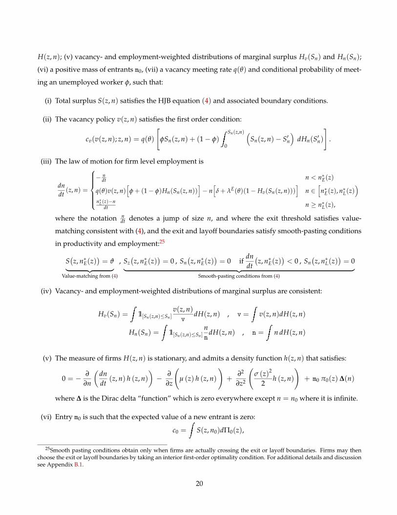
H(z, n); (v) vacancy- and employment-weighted distributions of marginal surplus Hv(Sn) and Hn(Sn);

(vi) a positive mass of entrants m0, (vii) a vacancy meeting rate q(θ) and conditional probability of meet-

ing an unemployed worker φ, such that:

(i) Total surplus S(z, n) satisfies the HJB equation (4) and associated boundary conditions.

(ii) The vacancy policy v(z, n) satisfies the first order condition:

cv(v(z, n); z, n) = q(θ)

[φSn(z, n) + (1− φ)

Sn(z,n)

0

(Sn(z, n)− S′n

)dHn(S′n)

].

(iii) The law of motion for firm level employment is

dndt

(z, n) =

− n

dt n < n∗E(z)

q(θ)v(z, n)[φ + (1− φ)Hn(Sn(z, n))

]− n

[δ + λE(θ)(1− Hv(Sn(z, n)))

]n ∈

[n∗E(z), n∗L(z)

)n∗L(z)−n

dt n ≥ n∗L(z),

where the notation ndt denotes a jump of size n, and where the exit threshold satisfies value-

matching consistent with (4), and the exit and layoff boundaries satisfy smooth-pasting conditions

in productivity and employment:25

S(z, n∗E(z)

)= ϑ︸︷︷︸

Value-matching from (4)

, Sz(z, n∗E(z)

)= 0 , Sn

(z, n∗E(z)

)= 0 if

dndt(z, n∗E(z)

)< 0 , Sn

(z, n∗L(z)

)= 0︸︷︷︸

Smooth-pasting conditions from (4)

(iv) Vacancy- and employment-weighted distributions of marginal surplus are consistent:

Hv(Sn) =

1[Sn(z,n)≤Sn]

v(z, n)v

dH(z, n) , v =

v(z, n)dH(z, n)

Hn(Sn) =

1[Sn(z,n)≤Sn]

nn

dH(z, n) , n =

n dH(z, n)

(v) The measure of firms H(z, n) is stationary, and admits a density function h(z, n) that satisfies:

0 = − ∂

∂n

(dndt

(z, n) h (z, n))− ∂

∂z

(µ (z) h (z, n)

)+

∂2

∂z2

(σ (z)2

2h (z, n)

)+ m0 π0(z) ∆(n)

where ∆ is the Dirac delta “function” which is zero everywhere except n = n0 where it is infinite.

(vi) Entry m0 is such that the expected value of a new entrant is zero:

c0 =

S(z, n0)dΠ0(z),

25Smooth pasting conditions obtain only when firms are actually crossing the exit or layoff boundaries. Firms may thenchoose the exit or layoff boundaries by taking an interior first-order optimality condition. For additional details and discussionsee Appendix B.1.

20

(vii) Vacancy meeting rate q(θ) and conditional probability of meeting an unemployed worker φ are

consistent with the aggregate matching function given employment n, unemployment (u = n− n),

and vacancies v.

The numerical procedure to compute the equilibrium of the model is described in Appendix II.

4.2 Firm dynamics, job reallocation and worker turnover: a phase diagram

We now can represent firm dynamics (entry and exit), job reallocation (net growth), and worker real-

location (hires and separations) in the (n, z)-space. Figure 5 describes the functions that determine the

stay/exit frontier n∗E(z), hire/layoff frontier n∗L(z), and the zero growth locus n∗ZG(z).

First, Panel (a) considers the model without a scrap value such that there is no endogenous exit.

From (5) the layoff frontier has slope dz/dn = −Snn/Szn. Therefore properties (P1) (Snn < 0) and (P3)

(Szn > 0), imply the layoff frontier is positively sloped. Recall from Figure 3 that, fractionally to the

left of the layoff frontier n∗L(z), Sn ≈ 0, so vacancy posting is low and the firm shrinks due to EE−

and EU flows. Therefore the zero growth locus along which dn = 0 must be located strictly to the left

of the layoff frontier. Between the zero-growth locus and the layoff frontier, firms hire but lose even

more workers, and so experience job destruction (JD). To the left of the zero-growth locus, marginal

surplus is sufficiently large that firms are successful in hiring and retaining workers, and so experience

job creation (JC). In all cases some endogenous separations through quits also occur, thus the model

generates both hires for shrinking firms and endogenous separations for growing firms. To the right of

the layoff frontier, firms fire workers, destroying jobs en masse, and in doing so jump back to the frontier.

Panel (b) introduces a positive scrap value which induces endogenous exit. First, let us ignore the

smooth-pasting conditions. From (5) the exit frontier would have slope dz/dn = −Sn/Sz. Therefore

properties (P1) (Sn > 0, Snn < 0) and (P2) (Sz > 0), imply the exit frontier would have a minimum at

Sn = 0, where it crosses the layoff frontier, increasing on either side.

The smooth pasting conditions modify this frontier. A necessary condition for optimal exit is that

Sn = 0: if marginal surplus was positive on the exit boundary (S = ϑ), then the firm could post vacancies

and increase S > ϑ, and hence would not want to exit. Now recall that by Property (P1), S is strictly

concave in n, but optimal layoffs imply Sn = 0 on the layoff boundary, implying that Sn is not zero again

away from the layoff frontier. Combined, these observations have two implications. First, firms do not

exit along the downward sloping section of the exit frontier in the Hire & JC region. Indeed, firms in

this region have very high marginal surplus and drift to the right. Second, firms cannot be located in the

part of the Hire & JD region with a red ×-mark. A firm located here would be headed toward exit with

21

z

0 n

Hire

Layoff

dn = 0

Stay & Layoff

(a) No endogenous exit (ϑ = 0)

z

0 n

Hire / Layoff

Stay / Exit

dn = 0

Layoff & JD

Exit

Hire & JC

Hire & JD

×

(b) Endogenous exit (ϑ > 0)

Figure 5: Exit, layoff and zero-growth frontiers in the (n, z)-space

Notes: This figure plots exit, layoff and zero-growth frontiers for two cases: without and with positive scrap value. It alsoincludes examples of hypothetical firm paths, in each case keeping productivity fixed. A firm (black dot) that begins in thelayoff region jumps to the layoff frontier, firing n − n∗S(z) workers. Subsequent declines in productivity smoothly move thefirm along the layoff frontier until, possibly, exit. A firm that is located in the hiring region smoothly converges toward thedn = 0 line by growing or shrinking.

Sn > 0, which violates optimality. As a result, to the right of the intersection of the zero-growth locus

and the S(z, n) = ϑ locus, the exit frontier is flat.

The stationary distribution of firms in the economy has support along the layoff frontier, and to its

left, with zero mass along the left exit frontier. Growing firms do not exit, but shrinking firms may experi-

ence productivity shocks that force them over the horizontal section of the exit frontier. All firms—except

those on the layoff frontier—post vacancies, and hire workers from employment and unemployment,

and lose workers to employment and unemployment.26 Finally, not depicted in the figure, the mass m0

of entrants is distributed according to Π0(z), along a vertical line at n = n0. Only those with a high

enough value of z keep operating.

4.3 Limiting economies

Our economy includes as special cases two well known frameworks for worker flows on the one hand,

and firm dynamics on the other.

26The results derived in Section 3.5 regarding gross flows fully describe employment dynamics of the firm when interior tothese boundaries. In particular, one can think of Figure 4 as describing gross firm hiring along a straight horizontal line drawnin the (n, z) space of Figure 5 and running from the exit to the layoff frontier.

22

4.3.1 Vanishing decreasing returns in production

In traditional search and matching models with random, on the job search, the constant returns to scale

assumption implies an indeterminate firm size distribution. These are models of jobs rather than firms,

with each job having match output y(z). Here we show that the Bellman equation (4) is a natural gener-

alization of expressions of firm value found in these settings.

Consider the limiting case of (4) when the function y is linear in n, y(z, n) = zn. Depending on

the form of the recruiting cost function, we obtain either the surplus representation in Lise and Robin

(2017) or a slight variant thereof. The formulation in Lise and Robin (2017) arises when vacancy costs

are independent of n, c(v, n) = c(v), and the scrap value is zero (no endogenous exit). Under these

assumptions (4) becomes affine in size, where the slope gives the value of an existing match and the

intercept gives the value of a vacancy:

ρS(z, n) = S0(z)+n× ρS(z) where

ρS(z) = y(z)− b− δS(z) + µ(z)Sz(z) +

σ2(z)2 Szz(z)

S0(z) = maxv q(θ)v[

φS(z) + (1− φ) S(z)

0

(S(z)− S′

)dHn(S′)

]− c(v)

These correspond to equations (3), (6) and (7) in Lise and Robin (2017). Since S is independent of n,

Hn(S′) = H(z). The rank of a firm on the job ladder is determined only by its exogenous productivity

z. The value of new jobs therefore depends block-recursively on the value of existing ones. In this limit,

firm size is irrelevant for joint surplus and the distribution of marginal surplus.

A similar limiting economy arises when the production function is linear, but vacancy costs are ho-

mogeneous of degree one in (v, n) and, again, the scrap value is zero. See Appendix C for details.

4.3.2 Vanishing frictions

We first consider the limit as matching efficiency goes to infinity in the absence of on the job search. We

then add on-the-job search and show that this is key for obtaining a version of Hopenhayn (1992) in the

limit. Formal proofs are in Appendix D.

Frictionless limit without on-the-job-search. Let A be a scalar in front of the matching function, and

take this parameter to infinity in an economy without on-the-job search (ξ = 0). Now consider the

free-entry condition

S(n0, z)dΠ0(z) = c0 and the Bellman equation for joint surplus,

ρS(n, z) = maxv

y(n, z)− bn− c(v)− δnS(n, z) + qvSn(n, z) + µ(z)Sz(n, z) +σ(z)2

2Szz(n, z) (9)

23

The only general equilibrium object in total surplus is q. Therefore there is a unique value of q, indepen-

dent of A, such that the free-entry condition holds. With q unaffected by the increase in A, firm vacancy

policies v(n, z) and firm dynamics conditional on entry remain the same, while the measure of firms ad-

justs such that q remains constant. Since there exists dispersion in the marginal product of labor for any

arbitrary A, then this dispersion continues to exist even in the limit. This limiting result differs from the

competitive equilibrium of a frictionless model in which all firms’ marginal products of labor are equal

and equated to the wage.27

Frictionless limit with on-the-job search. On-the-job search breaks this result, allowing equilibrium

q to increase. As A increases unemployment u still goes to zero but, with on-the-job search total units

of search efficiency remain positive s∞ = ξn. Meanwhile aggregate feasibility ensures that vacancies

v∞ remain finite. Hence in the limit θ∞ = s∞/v∞ is constant, and q = Aθ−(1−β)∞ increases in A. As

q increases, reallocation of labor via job-to-job quits accelerates. These quits cause marginal surplus to

increase at low-Sn origin firms and decline at high-Sn poaching firms, compressing the distribution of Sn

to a point.

Our main result, shown in Appendix D, is that in the limit as q goes to infinity, firm behavior is

described by the following Bellman equation, employment policy function and boundary condition:

ρS(z) = maxn

y(z, n)− nb + µ(z)Sz(z) +σ2(z)

2Szz(z) , yn

(z, n∗(z)

)= b , S(z) ≥ ϑ , (10)

This characterization contains three results. First, with infinitely fast reallocation, there is no dispersion

in marginal surplus in equilibrium and hence no surplus gained from on-the-job search. Second, be-

havior is as if firms choose their optimal size each instant, with all hires realized through immediate

job-to-job reallocation. Third, this implies the only state variable is z and the productivity-size distri-

bution is degenerate on (z, n∗(z)), along which marginal products are equalized. Thus the limit of our

model is isomorphic to Hopenhayn (1992) with respect to job reallocation, firm exit, and the expected

profits of entrants, which are zero net of entry costs.

We conclude by noting that this natural limiting behavior of our economy stands in stark contrast

to traditional search models with constant returns to scale. In bargaining and wage posting models, all

employment would go to the most productive firm.

27To draw an analogy, consider a comparative statics in the Hopenhayn (1992) model with respect to a parameter that doesnot directly enter the free entry condition. The effect is a change in the aggregate supply of labor and, thus, the mass of firms,but not their distribution. See also Kaas (2020).

24

5 Estimation

Having provided a qualitative discussion of the model, we now turn to its quantitative implications. To

that end, we estimate the model on U.S. data. Because the model is set and solved in continuous time,

we can construct correctly time-aggregated measures at any desired frequency.

5.1 Methodology

We make the following functional form assumptions. The production function is y(z, n) = znα. The

vacancy cost function is c(v, n) = c1+γ

( vn

)γ v, as in Kaas and Kircher (2015), such that the per-vacancy

cost is increasing in the vacancy rate. The matching function is Cobb-Douglas with vacancy elasticity β:

a worker meets a vacancy at rate f (θ) = Aθβ and a vacancy meets a worker at rate q(θ) = Aθ−(1−β). The

distribution of entrant productivity draws is Pareto with a minimum of one and shape parameter ζ. Log

productivity follows a random walk, d log z(t) = µdt + σdW(t). We add exogenous firm exit at rate d.

These assumptions leave 16 parameters to determine. We proceed in three steps.

Externally set or normalized. We normalize or set to standard values five parameters, as summarized

in Table 1A. The discount rate ρ implies an annual real interest rate of five percent. The elasticity of

the matching function β = 0.50 is based on standard values in the literature (Petrongolo and Pissarides,

2001). When solving the model we add a fixed cost of operation c f and set the scrap value ϑ to zero;

the two are isomorphic. Without loss of generality we are then able to normalize c f .28 From the first

order condition for vacancies (6) it is clear that we cannot identify c and A separately, so we normalize

c. Finally, we set employment of entering firms, n0, to one which we interpret as the labor input of the

entrepreneur or founder.

Estimated offline. We set three parameters to target directly three moments in the data, as summarized

in Table 1B. First, the entry cost c0 is pinned down by an average firm size of 23. The measure of active

firms m that delivers an average firm size of 23 when there is a unit measure of workers and a non-

employment rate of 10 percent is 0.90/23. While m is an equilibrium outcome, the fact that a higher m

decreases the value of entry through a tighter labor market implies a unique c0 that satisfies the free-entry

condition under a given m. Here, and throughout, we use a broader definition of the pool of job-seekers

than in the standard unemployment definition in the CPS. This accounts for the fact that a significant

28The argument that we can normalize c f to one has two pieces. First, for a given fixed cost c f , we can always choose anentry cost c0 that generates the desired mass of firms m, see below. Second, with Pareto initial draws of productivity followedby a random walk, a higher fixed cost simply scales the economy up.

25

Parameter Value Moment Data ModelA. Externally set/normalized parameters

ρ Discount rate 0.004 5% annual real interest rateβ Elasticity of matches w.r.t. vacancies 0.5 Petrongolo and Pissarides (2001)c f Fixed cost of operation 1 Normalizationc/(1 + γ) Scalar in the cost of vacancies 100 Normalizationn0 Size of entrants 1 Normalization

B. Estimated offlinem Number of active firms 0.043 Average firm size (BDS) 23.340 20.851d Exogenous exit rate 0.000 Exit rate, 1000–2499 empl. firms 0.002 0.002γ Vacancy cost elasticity 3.450 Vacancy filling rate vs. hiring rate 3.450 3.450

C. Internally estimatedµ Drift of productivity -0.001 Exit rate (annual) 0.076 0.076σ St.d of productivity shocks 0.016 St.d. of log empl. growth (annual) 0.420 0.354α Curvature of production 0.817 Empl. share of 500+ firms 0.518 0.527ζ Shape of entry distribution 11.844 JC rate, age 1 firms (annual) 0.247 0.255A Matching efficiency 0.195 Nonemployment rate 0.100 0.100ξ Relative search efficiency of employed 0.151 EE rate (quarterly) 0.048 0.041δ Exogenous separation rate 0.017 EN rate (quarterly) 0.056 0.055b Flow value of leisure 1.029 JD rate of incumbents (annual) 0.092 0.093

Table 1: Estimated parameters and targeted momentsNotes: Annual firm dynamics moments are from HP-filtered Census BDS data between 2011–2016, with the exception of thestandard deviation of annual growth rates, which is from Elsby and Michaels (2013). Quarterly worker flows are from HP-filtered Census J2J data between 2011–2016.

number of hires come directly from out of the labor force and some of our data sources (JOLTS and

Census J2J) do not identify whether the origin of hires or destination of separations is unemployment or

non-participation.29

Second, the exogenous exit rate d is pinned down by an annual exit rate of firms with 1000–2499

employees of 0.2 percent. Such firms may layoff workers, but never exit endogenously in the model, as

total surplus is far from the exit frontier.

Third, the vacancy cost elasticity γ is pinned down by the cross-sectional relationship between

vacancy- and vacancy-filling rates. In JOLTS microdata, Davis, Faberman, and Haltiwanger (2013) docu-

ment a nearly log-linear relationship between each of these and the hiring rate, which implies a log-linear

relation between them. In the model, these relationships are driven by marginal surplus. The follow-

ing cross-sectional relationship can be derived from the firm’s optimality condition, using a log linear

approximation that is valid for firms with small growth rates:

logv∗(z, n)

n≈ κ0 + κ1 log

(h∗(z, n)

v− κ2

), where γ =

1κ1

(11)

Firms with high marginal surplus post more vacancies per worker, and fill them more quickly as they

29Our definition of the non-employment rate is constructed as follows. The numerator equals the sum of the unemployed(FRED series UNEMPLOY) plus those out-of-the-labor-force who answer that they ‘currently want a job’ in the CPS (NIL-FWJN). The denominator equals the sum of the civilian labor force (CLF16OV) plus the same subgroup of those out-of-the-labor-force (NILFWJN). From 2011-2016 this ratio is, on average, just above 10 percent.

26

Figure 6: Vacancy rates by firm gross hiring rate

Notes Data: Establishment-month observations in JOLTS microdata 2002-2018 are pooled in bins, where bins are determinedby net monthly growth rate, and have a width of 1 percent. Growth rates computed as in Davis, Faberman, and Haltiwanger(2013). Within bin b, total hires hb, total vacancies vb, total employment nb are computed. From these, the gross hiring ratehb/nb, and implied daily vacancy posting rate vrb = vb/(nb) are computed using the daily recruiting model of Davis, Faber-man, and Haltiwanger (2013). Model: The variables are constructed in the same way as in the data. Points plotted are logs ofthese variables, differenced about the bin representing a one percent net growth rate.

can poach labor from more firms. We compute these objects in JOLTS microdata in narrow monthly

growth rate bins, then estimate (11) by non-linear least squares.30 Our estimates imply γ = 3.45. Figure

6 shows this value for the vacancy cost elasticity provides a good fit to the microdata.

Internally estimated. The remaining parameters are estimated by minimizing the objective function

G(ψ) =(

m−m(ψ))′

W−1(

m−m(ψ))

, ψ =

µ, σ, α, ζ, A, ξ, δ, b

,

where m is a vector of empirical moments and m(ψ) are their model counterpart. The matrix W con-

tains squares of the data moments on the main diagonal and zeros elsewhere.31 We target eight moments

that are relatively standard to firm dynamics and frictional labor market literatures. While this remain-

ing subset of parameters is jointly estimated, some moments are particularly informative about some

parameters. Next, we briefly outline our logic.

The drift of productivity, µ, is informed by the (unweighted) firm exit rate. The more negative the

drift, the faster firms exit. The standard deviation of productivity shocks, σ, is informed by the standard

deviation of annual log employment growth. If shocks are larger, employment is more volatile. Decreas-

30We use establishment-month observations in JOLTS microdata 2002–2018 (see Mongey and Violante, 2019). As in Davis,Faberman, and Haltiwanger (2013), we pool all vacancies, hires and employment in net monthly growth rate bins of onepercent width. We then use these to compute the vacancy rate and vacancy yield at the bin level. To be consistent with ourapproximation we use growth rate bins between 2.5 and 9.5 percent when estimating (11).

31Our moments are taken from various data sources and in most instances we cannot compute variances of the moments,let alone covariances with other moments.

27

Figure 7: Distribution of firms and employment by firm age and size in data and model

Source: Census BDS

ing returns, α, is informed by the employment share of firms with more than 500 employees. A smaller

span of control allows for fewer large firms. The thickness of the tail of the productivity distribution of

entrants, ζ, is informed by job creation among young firms (Decker, Haltiwanger, Jarmin, and Miranda,

2020).32 Matching efficiency, A, is informed by the nonemployment rate, as a more efficient labor market

reduces nonemployment. Relative search efficiency of employed workers, ξ, and the exogenous separa-

tion rate, δ, are informed by quarterly EE and EN rates. Finally, the flow value of leisure, b, is informed

by the job destruction rate of incumbent firms. The direct effect of b on marginal surplus Sn(n, z) is one-

for-one, so under a higher b, a productivity shocks is more likely to lead a firm to hit the layoff frontier

Sn(n, z) = 0, and destroy jobs. Table 1C summarizes the parameters estimated by minimum distance. In

Appendix E we discuss identification more formally, and plot the marginal effect of each parameter on

its associated target moment and on the objective function.

5.2 Model fit

The estimated model is consistent with micro data that was not directly targeted by the estimation. This

data sits at the intersection of firm and worker dynamics: (i) the distribution of firms and employment,

(ii) job and worker flows across the distribution, and (iii) patterns of net poaching across the distribution.

32A natural alternative would have been to target the productivity gap between entrants (younger than 1 year old) andincumbents. The model does well in this respect. At the estimated parameter vector, this gap is 27 (35) percent in the model(data) (Gavazza, Mongey, and Violante, 2018).

28

A. Job, worker and firm reallocation by age

B. Job, worker and firm reallocation by size

Figure 8: Job, worker and firm reallocation by size and ageNotes: Data: Census BDS firm data for annual job creation, job destruction and exit. Quarterly rates constructed by dividingby four. Census J2J firm data for quarterly hiring and separation rates. Authors aggregate data into bins given in table whichreflect the granularity of J2J data. Census J2J separations (hires) include separations to (hires from) non-employment. Model:Time aggregated to a quarterly frequency.

1. Distribution of firms and employment. Figure 7 shows that the model reproduces the skewed

firm size and age distributions. In both data and model, around 90 percent of firms are small (less

than 20 employees), but these firms account for only around 20 percent of employment. Symmetrically,

firms with more than 500 employees represent less than 1 percent of firms, but more than 50 percent of

employment. By age, around half of firms are older than 10 years, but these account for 80 percent of

employment in the data, and somewhat more in the model.

2. Firm, job and worker reallocation. Figure 8 examines turnover at the level of firms, jobs and work-

ers. As in the data the rate of job creation peaks for young firms and then declines with age, while job

destruction rates are relatively flat. The model is also consistent with the mild decline in job turnover by

29

Figure 9: Net poaching and marginal surplus distribution

Notes: Panel A. Net poaching rate p(Sn) by log marginal surplus Sn and the CDF of log marginal surplus. Panel B. Decompo-sition of the change in net poaching rate as Sn rises into three components: (i) higher vacancies (red line), (ii) more poachinghires due to higher rank on the job ladder (green line), and (iii) lower poaching separations due to higher rank on the job ladder(blue line).

size. Not shown in the figure, in the data (model) 16 percent (15 percent) of all jobs are created by new

firm births and 28 percent (26 percent) by firms less than 10 years old. In terms of worker flows, EE tran-

sitions allow the model to account for the key fact that worker reallocation rates are around three times

as large as job reallocation rates, thus generating the right amount of churning. In the cross-section, the

model can reproduce the stark negative empirical relationship between hiring rates and firm age, but

struggles to match the gradient at which the separation rate declines with age in the data after age 3. The

model is also in line with the mild decline in worker turnover by size. The model reproduces the negative

gradient for firm exit with respect to age observed in the data. Absent jumps in the productivity process,

firms slowly shrink before exiting, and so every firm above medium size only exits exogenously: as a

result, the model matches small and very large firm exit rates, but not those of intermediate size firms.

3. Net poaching by firm characteristics. Figure 9A plots the distribution of marginal surplus H(Sn) to-

gether with the net poaching rate as a function of marginal surplus. The CDF reveals that the equilibrium

density h(Sn) is quite dispersed. Net poaching is flat and negative at the low end of the distribution of

Sn, after which it starts increasing steadily. What explains this particular shape? Under our assumptions

on vacancy costs, the vacancy rate of the firm (v = v/n) depends only on marginal surplus.33 The net

poaching rate p(Sn) is therefore:

p(Sn) = v(Sn)q(θ)(1− φ)Hn(Sn)− λE(θ)Hv(Sn).

33To see this note that the marginal cost of a vacancy is cv(v, n) ∝ (v/n)γ and, as characterized in Section 4, the marginalbenefit of a vacancy depends only on Sn.

30

Higher marginal surplus increases net poaching through three channels: (i) a higher return to vacancies

leads to higher vacancy posting, increasing EE hires (↑ v(Sn)); (ii) conditional on a vacancy, a greater

fraction of meetings result in a hire (↑ Hn(Sn)); (iii) firm incumbents match with fewer competitors that

result in an EE quit (↓ Hv(Sn)). Figure 9B plots these three forces using the following decomposition:

p(Sn) =

Sn

0

∂v(u)∂u

q(θ)(1− φ)Hn(u)du︸︷︷︸Increasing ↑ v(Sn)

+

Sn

0v(u)q(θ)(1− φ)hn(u)du︸︷︷︸

Increasing ↑ Hn(Sn)

− λE(θ)Hv(Sn)︸︷︷︸Decreasing ↓ Hv(Sn)

Firms with very low marginal surplus do not hire and lose all their employees who meet other firms,

so net poaching for them approaches −λE(θ). In the middle range of log Sn a rise in marginal surplus

increases firms’ net poaching mostly through changes in its marginal surplus rank which, in turn, ex-

pands hires from other firms (EE+) and reduces quits (EE−). The vacancy rate initially rises slowly, but

as firms get toward the top of the job ladder, vacancies are the only way to keep growing. This explains

why net poaching keeps rising even in the region where the CDF is flattening out, over which poaching

translates into negligible jumps up the ladder.

We now project this relationship between net poaching and marginal surplus onto observables in

order to compare model and data. Haltiwanger, Hyatt, Kahn, and McEntarfer (2018) document two key

empirical patterns: (i) a negligible gradient of net poaching by size, which is inconsistent with wage

posting models, and (ii) a steeper negative gradient by age, as young poach from old. Panels A and B

of Figure 10 show that the model matches these patterns quite well, albeit the slope by age is somewhat

more pronounced in the model relative to the data. Size is not a particularly good predictor of where

a firm sits on the marginal surplus job ladder. Consider a vertical slice of Figure 5. At a given size

some firms are highly productive, have a high Sn, have positive net poaching and create jobs on net.

Meanwhile, other firms are less productive, have a low Sn, negative net poaching and destroy jobs on

net. In contrast, young firms are on average small and productive: they sit to the left of dn = 0 and,

having not yet grown, are high on the marginal surplus job ladder. They therefore display large and

positive net poaching rates.34

Panels C and D of Figure 10 plots net poaching rates as a function of two other, potentially, observ-

able firm characteristics, labor productivity and net employment growth rate. The model predicts a

much higher gradient between these two variables and net poaching rates compared to size and age.

First, marginal surplus is highly correlated with the static marginal product of labor, and the latter is

34Put differently, the reason why small firms do not have high net poaching rates on average is because some of themare young and highly productive, but did not have had time to grow yet, while others are small simply because they areunproductive.

31

Figure 10: Net poaching rates by size, age, labor productivity and net employment growth rate

Notes: In panels C and D, firms are ranked according to the employment weighted distribution of labor productivity (C) andemployment growth (D).

proportional to the average product under our functional form for y(z, n).35 Second, both in the data

and in the model, hires from employment account for much of firm employment growth. This implies a

tight positive relation between net growth rate and net poaching rate.

6 Search frictions and labor misallocation

It is search and matching frictions, in our model, that impede the instantaneous reallocation of labor

across firms. In this section we analyze and quantify the implications of this source of misallocation along

three dimensions of the data: cross-section, firm life-cycle and the aggregate business cycle. Because our

model is consistent with micro data on both the speed and the direction of the poaching flows across

firms that resolve misallocation, it offers a credible platform for these three exercises.

6.1 Misallocation cost of labor market frictions

Our model puts us in a unique position to quantify such misallocation by computing the limit as search

frictions vanish. This exercise would not make sense in a model without decreasing returns since it

35One generalization of the model that would weaken this relation is the addition of heterogeneity in the scale of productionparameter α, as in Gavazza, Mongey, and Violante (2018). This would create an additional source of cross-sectional variationin marginal surplus that is orthogonal to z. Another one is the addition to the model of forced EE moves (‘godfather shocks’).

32

Figure 11: Frictionless limit: the effect of increasing match efficiency

would predict that the most productive firm would hire the entire labor force. Conversely, we have

shown that our economy converges to a competitive equilibrium with a non-degenerate firm size distri-

bution.

Our counterfactual experiment shifts the value of matching efficiency A holding all other parameters

fixed at our baseline calibration. Figure 11 plots model outcomes for a wide range of values for A. As

frictions vanish, non-employment falls, the dispersion of marginal products across firms shrinks toward

zero, the correlation between size and productivity rises toward one, and aggregate output grows.36

To isolate the role of misallocation, we decompose the change in output into a component due to

the allocation of workers across firms, and a component due to more employment in the economy as a

whole, the scale effect. Imposing an aggregate production function Y = Znα, then across steady states

∆ log Y = ∆ log Z + α∆ log n , Z :=N×Z

z(nn

)αdH(n, z).

The TFP term Z captures misallocation and is constant if the distribution of employment across firms is

unchanged.37 The misallocation from labor market frictions is sizable. For example, reducing frictions

to an extent that cuts the non-employment rate by half (from 10 to 5 percent) raises aggregate TFP by

36Output is net of vacancy costs. Note that the relationship between frictions and output is concave because the non-employment rate is convex in match efficiency.

37In a constant returns to scale economy in the limit Z = max z, since all employment is at the firm with the highestproductivity.

33

3 percent and output by 7 percent, such that reallocation accounts for nearly half the gains in output.

A five-fold rise in match efficiency relative to the benchmark would virtually eliminate frictional non-

employment and boost TFP permanently by 5 percent.

6.2 Misallocation and the life cycle of superstar firms

The addition of labor market frictions to a firm dynamics model overcomes a notable shortcoming of

competitive environments first identified by Luttmer (2011). When these models are calibrated to gen-

erate the correct cross-sectional variation in firm employment growth rates and the empirical size distri-

bution of firms, they imply that the median age of ‘superstar’ firms (n > 10, 000 workers) is 750 years.

In the data, the median age of such firms is only about 75 years.38

The root of the problem is that in the data young firms are almost uniformly small and firm em-

ployment volatility is not that large. Viewed through the lens of a frictionless model where size and

productivity are perfectly correlated, young firms must be low productivity. This moment is therefore

matched by young firms being way out in the left tail of the productivity distribution. If shocks are

driven by a geometric Brownian motion and chosen to match the empirical volatility of firm growth,

then only small shocks are required. Combined this means that it takes a very long time for any firm to

get from the left to the very right tail of the productivity distribution and hence become a superstar firm.

In our environment, instead, labor market frictions imply that some young firms can be extremely

productive but still small as frictions have prevented them from immediately growing large. Because

their initial productivity is already near the upper tail, they remain at the top of the job ladder even

after hiring many workers. This makes expansion cheap, and accommodates rapid growth. They can

therefore move relatively quickly to the tail of the size distribution. When we simulate firm life cycles

in the model, we find that the median age of firms with more than 10,000 workers is 110 years, and

hence much closer to the data. It is thus the existence of labor misallocation—high productivity, but

small size—that allows the model to be consistent with the cross-sectional size distribution and life-cycle

growth trajectories.

6.3 Misallocation in the Great Recession

The Great Recession provided a raft of new facts regarding the cyclical reallocation of workers across

firms. In particular the two key mechanisms through which labor gets reallocated across productive

38For description of data see Luttmer (2011), Appendix A: data was collected for 2008, on 813 firms with 10,000 or moreworkers, with the data of incorporation taken from a variety of historical sources, for example, Mergent Online database.

34

Figure 12: Entry and job-to-job hiring rates over the Great Recession: Aggregate and Cross-section

Notes: Both panels are constructed from the same data at the metro level. Establishment entry and number of establishmentsare from the Census BDS data, and used to construct establishment entry rate. Job-to-job hires and employment are from theCensus J2J data, and used to construct EE hire rate. The data cover the subset of states that participate in these Census datarelease programs. These cover more than half of the US population.

units are (i) the entry of new firms which replace unproductive exiting firms and (ii) the upward move-

ment of workers up the job ladder toward more productive firms. During the Great Recession both

mechanisms slowed considerably. Firm entry (measured as the number of firms less than 1 year old in

the BDS) dropped by almost 30 percent between 2007 and 2009 and has since recovered very slowly.

Even allowing for the secular decline in firm entry documented by Pugsley and Sahin (2019), the drop

around the Great Recession would be at least 20 percent.39 The EE rate also fell markedly over the same

period (Figure 12A).40

The decline in job-to-job transitions implied a tapering in the process of upgrading from low- to

high-rank firms. Haltiwanger, Hyatt, Kahn, and McEntarfer (2018) document a fall in net poaching of

high wage firms, those who are presumably at the top of the job ladder. Similarly, Moscarini and Postel-

Vinay (2016) use a structural model to rank firms on the job ladder and estimate that high-rank firms

disproportionately curtailed their demand for new labor in the recession. In short, as they put it: the job

ladder failed, starting from the upper rungs.

39The entry rate in Figure 12A is for establishments for consistency with panel B which is constructed at the city level forwhich there are no firm-level data. The percentage fall in entry rates of firms and establishments in 2008-2009 is very similarand over the last 40 years the correlation between the two series is 0.98.

40The exact size of this decline is still debated. Haltiwanger, Hyatt, Kahn, and McEntarfer (2018) use Census J2J data andreport a decline around 30 percent, which Figure 12 replicates. Fujita, Moscarini, and Postel-Vinay (2019) argue that Censusdata overestimate this drop because employment status is only measured quarterly and spurious poaching transitions (EE fromquarter to quarter, but with an ‘invisible’ non-employment spell in between) were much less likely during the recession, whenunemployment spells were quite long. When they reassess measurement error in CPS data, these authors estimate a drop inthe EE rate around 15 percent.

35

To date, these two facts have not been connected in the literature, since there is a paucity of quan-

titative structural models that can integrate firm dynamics with on-the-job search. Theoretically, our

environment suggests a natural link between the two, and since our model matches key data on firm

and worker dynamics we can also test this link quantitatively.

Theoretically, the mechanism is as follows. New entrants and young firms account for a sizable share

of vacancies and have higher marginal surplus than other firms in the economy. Following a shock that

leads to a drop in the number of entrants, poaching would fall at the top of the ladder which reduces

worker reallocation through the middle of the ladder, and so on down to unemployment.

Empirically, this idea is consistent with cross-city patterns. Figure 12B combines newly released

Census J2J data with Census BDS data at the metro level. The time-series decline in entry and job-to-job

mobility is mirrored in the cross-section of labor markets: cities with larger declines in establishment

entry were associated with larger declines in job-to-job mobility.

We now simulate the Great Recession in our model. The aggregate shock that best describes the Great

Recession is one that worsens financial conditions. To proxy for a financial shock in our framework, we

solve the model under an unexpected temporary increase in the discount rate ρ (as in Hall, 2017). We cal-

ibrate the initial jump and the rate of convergence of ρ to match the 5 ppt increase in the unemployment

rate and the seven years it took to return to pre-recession levels.

Because the focus is on short-run dynamics, we replace the long-run free-entry condition with a

simple imperfectly elastic entry rule. We posit that every instant, a measure 1 (a normalization) of en-

trepreneurs contemplate entering. They draw preference shocks for opening a new firm (ε1) and for

taking an outside option (ε2) normalized to deliver a payoff of 1. Thus, entrepreneurs solve

max

ε1 ×St

c0, ε2 × 1

where St =

St(z, n0)dΠ0(z) denotes the expected surplus at firm entry. We assume that εi are Frechet

distributed with shape parameter θ and scale normalized to 1. The measure of new firms at t satisfies:

Mt =Sθ

t

Sθt + cθ

0

We set θ = XYZ to match the observed decline in firm entry (-30%) following the discount rate shock.

Figure 13 describes the response of the model economy to the shock. The shock lowers the valuation

of future revenues at all firms, and as a result, average surplus falls. Young firms have a disproportion-

ate fraction of their revenues in the future so are especially hard hit, causing entry to collapse. Marginal

36

Figure 13: Response of the economy following a discount rate shock

surplus also falls, which causes an endogenous spike in EU separations. Both lead to a jump in unem-

ployment. Furthermore, declining marginal surplus reduces the return on vacancies (7), so aggregate

vacancies collapse, job creation contracts, and UE hires decline. This leads the jump in unemployment

to persist. With less vacancies and more unemployed workers, the aggregate vacancy yield rises. As in

the data, the rise in the vacancy yield is more pronounced for small firms (Moscarini and Postel-Vinay,

2016). For small unproductive firms at the bottom of the ladder, unemployment is the main source of

hiring, so as the pool of unemployed job seekers expands, the vacancy filling rate of these firms jumps.

Quantitatively, the experiment matches key non-targeted moments: entry declines by almost 30 per-

cent, the EE rate falls about one third and vacancies contract by 50 percent (Gavazza, Mongey, and

Violante, 2018). The decline in output is 6.5 percent and 9 percent in the data (Fernald, 2014).

We now turn to the dynamics of the job ladder. In the aggregate, the job-to-job mobility rate drops

upon impact and slowly recovers. In the cross-section, the shift in the vacancy distribution away from

high marginal surplus firms—whose poaching rates were most sensitive to their vacancy rates (recall

Figure 9B)—causes poaching rates to collapse at high marginal surplus firms and, symmetrically, grow

at low-marginal surplus firms. This compositional effect reduces the probability that a worker moves

37

from a low- to a high-marginal surplus firm, causing the observed ‘failure’ of the job ladder.

Throughout the recession and its protracted recovery, the slowdown of worker flows towards high-

marginal surplus firms exacerbates the misallocation that arises from labor market frictions. This force

grinds down aggregate TFP, and is responsible for about a quarter of the decline in output. The recov-

ery of aggregate productivity is sluggish, with the scars of the recession encoded in the slow moving

dynamics of the distribution of employment across firms.

7 Conclusion

We have set out a new framework to jointly study firm entry and exit, job reallocation, and worker

turnover, both through non-employment and through direct job-to-job transitions, in a frictional labor

market. The novel feature of the environment, which makes the problem challenging in the presence of

random on-the-job search, is diminishing returns to scale in the firm’s technology –the hallmark of classic

theories of the firm size distribution based on the idea of ‘span of control’. By extending the contractual

environment of Postel-Vinay and Robin (2002), we obtain a tractable ‘joint value’ representation that

reduces a potentially unmanageable state space to a very parsimonious one. In contrast with search

existing models with linear technology that display a job ladder in exogenous productivity, our model

features an endogenous job ladder in marginal surplus. Canonical search models and competitive firm

dynamics models are special cases of our environment.

We illustrated how to use a calibrated version of the model as a laboratory to shed light on the

role of labor misallocation due to search and matching frictions in the cross-section, firm life cycle, and

aggregate time series dimension.

Our framework is quite flexible and can be extended in a number of directions while retaining

tractability (i.e., a parsimonious state space). For example, an isomorphic representation of our firm

problem is constant returns to scale in production of a differentiated final good, which would yield a

decreasing marginal revenue as under monopolistic competition. We can therefore easily accommodate

imperfect substitutability in the goods market which is a key ingredient of trade models and macroeco-

nomic models with nominal rigidities in goods markets.

The model can also integrate heterogeneity in the scale of production across firms (e.g. to allow

for fast-growing ‘gazelle’ firms) and fixed heterogeneity in worker types to address sorting within and

across firms. It is also straightforward to introduce firm-level amenities which have been documented

to be important to describe sorting patterns in the data (Sorkin, 2018). Once wage determination is

incorporated into the model —a task we left to future work— shocks to firm-specific or general human

38

capital can also be accommodated to study earnings dynamics within firms and along worker careers.

In all these cases the joint-value representation remains valid and, as long as heterogeneity is discrete

and of moderate dimension, the cardinality of the state vector remains manageable. As is, the model

can be used to study the effect of most labor market policies (e.g., unemployment benefits, severance

payments, firing taxes and hiring subsidies) on firm dynamics, worker reallocation and aggregate em-

ployment and output.

Stationary equilibrium and transitional dynamics can be computed very efficiently and, albeit not in

the paper, incorporating aggregate shocks using the approach of Boppart, Krusell, and Mitman (2018) is

straightforward which makes business cycles analysis possible.

In ongoing work (Bilal, Engbom, Mongey, and Violante, 2021), we show how one can combine this

framework with a creative-destruction model of endogenous growth and revisit the nexus between the

speed of technical change and aggregate employment (Aghion and Howitt, 1994) in the context of the

recent growth slowdown and decline in labor market dynamism. Differently from the canonical mod-

els in the endogenous growth literature where optimal size is reached instantaneously, in this hybrid

model building to the optimal productive capacity and replacing less productive incumbents is a slow

process for an innovator, which requires poaching workers away from other firms. As a result, creative

destruction can induce more labor misallocation.

In sum, with the introduction of a well defined notion of firm boundaries (through decreasing returns

in technology or downward sloping demand) into a comprehensive model of frictional labor reallocation

across firms, our framework can be potentially useful to study a number of questions in growth, business

cycle analysis, labor and trade.

39

References

ACEMOGLU, D. (2001): “Good jobs versus Bad Jobs,” Journal of Labor Economics, 19(1), 1–21.

ACEMOGLU, D., AND W. B. HAWKINS (2014): “Search with Multi-Worker Firms,” Theoretical Economics, 9(3), 583–628.

AGHION, P., AND P. HOWITT (1994): “Growth and Unemployment,” The Review of Economic Studies, 61(3), 477–494.

ARELLANO, C., Y. BAI, AND P. KEHOE (2019): “Financial Frictions and Fluctuations in Volatility,” Journal of PoliticalEconomy, 127(22990), 2049–2103.

AUDOLY, R. (2019): “Firm Dynamics and Random Search over the Business Cycle,” Discussion paper, UniversityCollege London.

BERTOLA, G., AND R. J. CABALLERO (1994): “Cross-Sectional Efficiency and Labour Hoarding in a MatchingModel of Unemployment,” Review of Economic Studies, 61(3), 435–56.

BILAL, A., N. ENGBOM, S. MONGEY, AND G. L. VIOLANTE (2021): “Labor Market Dynamics When Ideas areGetting Harder to Find,” Discussion paper.

BILAL, A., AND H. LHUILLIER (2021): “Outsourcing, Inequality and Aggregate Output,” Discussion paper, Har-vard University.

BOPPART, T., P. KRUSELL, AND K. MITMAN (2018): “Exploiting MIT Shocks in Heterogeneous-agent Economies:the Impulse Response as a Numerical Derivative,” Journal of Economic Dynamics and Control, 89, 68–92.

BOROVICKOVÁ, K. (2016): “Job flows, Worker Flows and Labor Market Policies,” Discussion paper, New YorkUniversity.

BREKKE, AND OKSENDAL (1990): “The High Contact Principle as a Sufficiency Condition for Optimal Stopping,”Preprint series: Pure mathematics.

BRÜGEMANN, B., P. GAUTIER, AND G. MENZIO (2018): “Intra Firm Bargaining and Shapley Values,” The Reviewof Economic Studies, 86(2), 564–592.

BURDETT, K., AND D. MORTENSEN (1998): “Wage Differentials, Employer Size, and Unemployment,” InternationalEconomic Review, 39(2), 257–273.

CLEMENTI, G., AND D. PALAZZO (2010): “Entry, Exit, Firm Dynamics, and Aggregate Fluctuations,” Discussionpaper, New York University.

COLES, M., AND D. MORTENSEN (2016): “Equilibrium Labor Turnover, Firm Growth, and Unemployment,”Econometrica, 84, 347–363.

DAVIS, S. J., R. J. FABERMAN, AND J. C. HALTIWANGER (2013): “The Establishment-Level Behavior of Vacanciesand Hiring,” Quarterly Journal of Economics, 128(2), 581–622.

DECKER, R. A., J. C. HALTIWANGER, R. S. JARMIN, AND J. MIRANDA (2020): “Changing Business Dynamismand Productivity: Shocks vs Responsiveness,” American Economic Review, 110(24236), 3952–3990.

DIAMOND, P. A., AND E. MASKIN (1979): “An Equilibrium Analysis of Search and Breach of Contract, I: SteadyStates,” Bell Journal of Economics, 10(1), 282–316.

ELSBY, M., AND A. GOTTFRIES (2021): “Firm Dynamics, On-the-Job Search and Labor Market Fluctuations,” Re-view of Economic Studies (forthcoming).

40

ELSBY, M. W. L., AND R. MICHAELS (2013): “Marginal Jobs, Heterogeneous Firms, and Unemployment Flows,”American Economic Journal: Macroeconomics, 5(1), 1–48.

ELSBY, M. W. L., R. MICHAELS, AND D. RATNER (2019): “The Aggregate Effects of Labor Market Frictions,”Quantitative Economics, 10(3), 803–852.

ENGBOM, N. (2017): “Firm and Worker Dynamics in an Aging Labor Market,” Discussion paper, New York Uni-versity.

FERNALD, J. G. (2014): “Productivity and Potential Output before, during, and after the Great Recession,” inNBER Macroeconomics Annual, ed. by J. A. Parker, and M. Woodford, vol. 29, pp. 1–51. Chicago, IL: University ofChicago Press.

FUJITA, S., G. MOSCARINI, AND F. POSTEL-VINAY (2019): “Measuring Employer-to-Employer Reallocation,” Dis-cussion paper, Yale University.

FUJITA, S., AND M. NAKAJIMA (2016): “Worker Flows and Job Flows: A Quantitative Investigation,” Review ofEconomic Dynamics, 22, 1–20.

GAVAZZA, A., S. MONGEY, AND G. L. VIOLANTE (2018): “Aggregate Recruiting Intensity,” American EconomicReview, 108(8), 2088–2127.

GOUIN-BONENFANT, E. (2018): “Productivity Dispersion, Between-Firm Competition, and the Labor Share,” Dis-cussion paper, University of California San Diego.

HALL, R. E. (2017): “High Discounts and High Unemployment,” American Economic Review, 107(2), 305–30.

HALTIWANGER, JOHN ANG HYATT, H. R., E. MCENTARFER, AND M. STAIGER (2021): “Cyclical Worker Flows:Cleansing vs. Sullying,” NBER Working Paper 28802, National Bureau of Economic Research.

HALTIWANGER, J. C., H. R. HYATT, L. B. KAHN, AND E. MCENTARFER (2018): “Cyclical Job Ladders by FirmSize and Firm Wage,” American Economic Journal: Macroeconomics, 10(2), 52–85.

HAWKINS, W. B. (2015): “Bargaining with Commitment Between Workers and Large Firms,” Review of EconomicDynamics, 18(2), 350–364.

HOPENHAYN, H., AND R. ROGERSON (1993): “Job Turnover and Policy Evaluation: A General Equilibrium Anal-ysis,” Journal of Political Economy, 101(5), 915–938.

HOPENHAYN, H. A. (1992): “Entry, Exit, and Firm Dynamics in Long Run Equilibrium,” Econometrica, 60(5), 1127–50.

JAROSCH, G. (2021): “Searching for Job Security and the Consequences of Job Loss,” Discussion paper, NationalBureau of Economic Research.

KAAS, L. (2020): “Block-Recursive Equilibria in Heterogenous-Agent Models,” Discussion Paper 8737, CESifoWorking Paper.

KAAS, L., AND P. KIRCHER (2015): “Efficient Firm Dynamics in a Frictional Labor Market,” American EconomicReview, 105(10), 3030–60.

KIYOTAKI, N., AND R. LAGOS (2007): “A Model of Job and Worker Flows,” Journal of Political Economy, 115(5),770–819.

KLETTE, T., AND S. KORTUM (2004): “Innovating Firms and Aggregate Innovation,” Journal of Political Economy,vol. 112, no. 5](5), 986–1018.

41

LENTZ, R. (2015): “Optimal Employment Contracts with Hidden Search,” Discussion paper, University ofWisconsin-Madison.

LENTZ, R., AND D. MORTENSEN (2012): “Labor Market Friction, Firm Heterogeneity, and Aggregate Employmentand Productivity,” Discussion paper, University of Wisconsin.

LINDENLAUB, I., AND F. POSTEL-VINAY (2016): “Multidimensional Sorting Under Random Search,” Discussionpaper, Yale University.

LISE, J., AND J.-M. ROBIN (2017): “The Macrodynamics of Sorting between Workers and Firms,” American Eco-nomic Review, 107(4), 1104–1135.

LUCAS, R. E. (1978): “On the Size Distribution of Business Firms,” The Bell Journal of Economics, 9(2), 508.

LUTTMER, E. G. (2010): “Models of Growth and Firm Heterogeneity,” Annual Review of Economics, 2(1), 547–576.

LUTTMER, E. G. J. (2011): “On the Mechanics of Firm Growth,” Review of Economic Studies, 78(3), 1042–1068.

MACLEOD, W. B., AND J. M. MALCOMSON (1989): “Implicit Contracts, Incentive Compatibility, and InvoluntaryUnemployment,” Econometrica: Journal of the Econometric Society, pp. 447–480.

MENZIO, G., AND S. SHI (2011): “Efficient Search On the Job and the Business Cycle,” Journal of Political Economy,119(3), 468–510.

MONGEY, S., AND G. L. VIOLANTE (2019): “Macro Recruiting Intensity from Micro Data,” NBER Working Papers26231, National Bureau of Economic Research, Inc.

MOSCARINI, G., AND F. POSTEL-VINAY (2013): “Stochastic Search Equilibrium,” Review of Economic Studies, 80(4),1545–1581.

(2016): “Did the Job Ladder Fail after the Great Recession?,” Journal of Labor Economics, 34(S1), S55–S93.

PESKIR, AND SHIRYAEV (2006): Optimal Stopping and Free Boundary Problems. Basel: Birkhauser.

PETRONGOLO, B., AND C. A. PISSARIDES (2001): “Looking into the black box: A survey of the matching function,”Journal of Economic literature, pp. 390–431.

PHAM (2009): Continuous-Time Stochastic Control and Optimization with Financial Applications. Berlin, Heidelberg:Springer.

POSTEL-VINAY, F., AND J.-M. ROBIN (2002): “Equilibrium Wage Dispersion with Worker and Employer Hetero-geneity,” Econometrica, 70(6), 2295–2350.

POSTEL-VINAY, F., AND H. TURON (2010): “On-the-job Search, Productivity Shocks, and the Individual EarningsProcess,” International Economic Review, 51(3), 599–629.

PUGSLEY, B. W., AND A. SAHIN (2019): “Grown-up Business Cycles,” The Review of Financial Studies, 32(3), 1102–1147.

SCHAAL, E. (2017): “Uncertainty and Unemployment,” Econometrica, 85(6), 1675–721.

SEDLÁCEK, P. (2020): “Lost Generations of Firms and Aggregate Labor Market Dynamics,” Journal of MonetaryEconomics, 111, 16–31.

SHIMER, R. (2005): “The Cyclical Behavior of Equilibrium Unemployment and Vacancies,” American EconomicReview, 95(1), 25–49.

42

SIEMER, M. (2014): “Firm Entry and Employment Dynamics in the Great Recession,” Finance and EconomicsDiscussion Series 2014-56, Board of Governors of the Federal Reserve System.

SORKIN, I. (2018): “Ranking Firms Using Revealed Preference,” The Quarterly Journal of Economics, 133(3), 1331–1393.

STOKEY (2009): The Economics of Inaction : Stochastic Control Models with Fixed Costs. Princeton, NJ: Princeton Uni-versity Press.

STOLE, L. A., AND J. ZWIEBEL (1996): “Intrafirm Bargaining under Non-Binding Contracts,” Review of EconomicStudies, 63(3), 375–410.

43

APPENDIX I - FOR ONLINE PUBLICATION

Firm and Worker Dynamics in a Frictional Labor Market

Adrien Bilal, Niklas Engbom, Simon Mongey, Gianluca Violante

This Appendix is organized as follows. Section A provides intuition for how our assumptions (A) yield

a tractable Bellman equation for joint value. Section B provides a characterization of the surplus func-

tion. Section C derives an alternative limit of the Bellman equation for the joint value as decreasing

returns vanish. Section D derives the limiting behavior of our economy when frictions vanish. Section E

illustrates identification of the model.

A Static Example

Set up. Consider a firm with decreasing returns to scale technology y(z, n) such that y(z, 0) = 0. Sup-

pose the firm starts with productivity z and n = 1 worker. The current contract between the firm and

the incumbent specifies a wage w1 ∈ (b, y(z, 1)), where b = U is the value of unemployment. At this

point, the incumbent worker does not have a credible threat to quit into unemployment nor the firm has

a credible threat to fire the worker. Then, the labor market opens. For now we also assume that the firm

has sunk the cost of a vacancy c. Later we explicitly consider the decision to post a vacancy.

A.1 UE hire

We describe how to obtain the ‘UE hire’ term in (1). Assume the firm’s vacancy meets an unemployed

worker. Four different cases can arise from the combination of hiring/not hiring and renegotiating/not

renegotiating the wage with the incumbent. Our assumption on external negotiation (A-EN) requires

that in all cases the take-leave wage offer of the firm to the outside worker is w2 = b. Our internal

negotiation assumption (A-IN) requires that the joint value with and without renegotiation is the same

and simply equals output y(z, n). Let w∗1 be the incumbent wage after the internal negotiation.

If the firm hires the new worker, its profits are as follows:

y(z, 2)− w1 − b︸︷︷︸Without renegotiation

, y(z, 2)− w∗1 − b︸︷︷︸With renegotiation

,

If the firm does not hire the new worker, its profits are

1

y(z, 1)− w1︸︷︷︸Without renegotiation

, y(z, 1)− w∗1︸︷︷︸With renegotiation

We now describe which case occurs. This requires understanding when our mutual consent assumption

(A-MC) coupled with limited commitment on layoffs (A-LC) bind. In particular, the firm may obtain a

credible threat to trigger renegotiation of w1. We focus first on when a hire occurs.

Hire. A hire without renegotiation occurs when the following two conditions hold:

y(z, 2)− w1 − b ≥ y(z, 1)− b︸︷︷︸No credible threat

, y(z, 2)− w1 − b ≥ y(z, 1)− w1︸︷︷︸Optimal to hire w/o renegotiation

(12)

The first condition illustrates that the threat to fire the incumbent worker is not credible, which under (A-

MC) implies no renegotiation. Keeping the incumbent worker at w1 and employing the outside worker

at b delivers a higher value to the firm than the threat of “swapping”: firing worker one and hiring

the unemployed worker in his place. Given no renegotiation, the second condition ensures hiring is

privately optimal for the firm.

A hire with renegotiation occurs when the following two conditions hold:

y(z, 2)− w1 − b < y(z, 1)− b︸︷︷︸Credible threat

, y(z, 2)− w∗1 − b > y(z, 1)− w∗1︸︷︷︸Optimal to hire w/ renegotiation

. (13)

The firm has now a credible threat to fire the incumbent worker according to (A-LC). This is possible

only under decreasing returns to scale: even though w1 < y(z, 1), the first inequality in (13) implies

w1 > y(z, 2) − y(z, 1), i.e. the incumbent wage is above its own marginal product. Employing the

outside worker at b and keeping the incumbent worker at w1 delivers a lower value than ‘firing and

swapping’. The second condition is necessary for hiring to be optimal under the renegotiated wage w∗1to the incumbent worker.

Under the zero sum game assumption (A-IN), the renegotiated wage w∗1 only redistributes value

between the incumbent worker and the firm, but does not affect total value.41 In addition, it must be

individually rational, and so w∗1 ∈ [b, y(z, 2) − y(z, 1)]. Without further assumptions we cannot say

where exactly the new wage lies within this interval, but we can nonetheless pin down allocations.

Rearranging the optimal hiring conditions, we observe that both are satisfied as long as

y(z, 2)− y(z, 1) > b. (14)

Note that without internal renegotiation (A-IN), the hiring condition would differ in the two cases. If

wages could not be cut and the firm had a credible threat, the incumbent worker would be fired and the

41Two relevant cases that would violate this condition are (i) if worker’s effort depends on the wage and enters the produc-tion function, and (ii) concave utility.

2

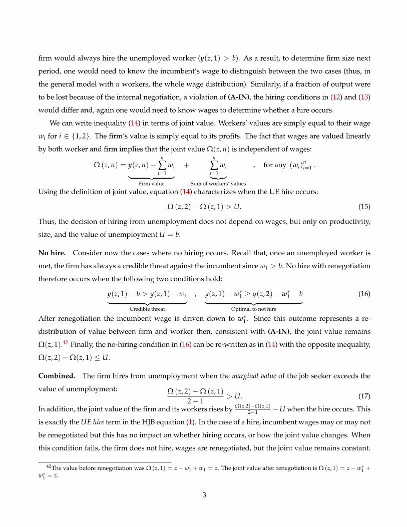
firm would always hire the unemployed worker (y(z, 1) > b). As a result, to determine firm size next

period, one would need to know the incumbent’s wage to distinguish between the two cases (thus, in

the general model with n workers, the whole wage distribution). Similarly, if a fraction of output were

to be lost because of the internal negotiation, a violation of (A-IN), the hiring conditions in (12) and (13)

would differ and, again one would need to know wages to determine whether a hire occurs.

We can write inequality (14) in terms of joint value. Workers’ values are simply equal to their wage

wi for i ∈ 1, 2. The firm’s value is simply equal to its profits. The fact that wages are valued linearly

by both worker and firm implies that the joint value Ω(z, n) is independent of wages:

Ω (z, n) = y(z, n)−n

∑i=1

wi︸︷︷︸Firm value

+n

∑i=1

wi︸︷︷︸Sum of workers’ values

, for any (wi)ni=1 .

Using the definition of joint value, equation (14) characterizes when the UE hire occurs:

Ω (z, 2)−Ω (z, 1) > U. (15)

Thus, the decision of hiring from unemployment does not depend on wages, but only on productivity,

size, and the value of unemployment U = b.

No hire. Consider now the cases where no hiring occurs. Recall that, once an unemployed worker is

met, the firm has always a credible threat against the incumbent since w1 > b. No hire with renegotiation

therefore occurs when the following two conditions hold:

y(z, 1)− b > y(z, 1)− w1︸︷︷︸Credible threat

, y(z, 1)− w∗1 ≥ y(z, 2)− w∗1 − b︸︷︷︸Optimal to not hire

(16)

After renegotiation the incumbent wage is driven down to w∗1 . Since this outcome represents a re-

distribution of value between firm and worker then, consistent with (A-IN), the joint value remains

Ω(z, 1).42 Finally, the no-hiring condition in (16) can be re-written as in (14) with the opposite inequality,

Ω(z, 2)−Ω(z, 1) ≤ U.

Combined. The firm hires from unemployment when the marginal value of the job seeker exceeds the

value of unemployment: Ω (z, 2)−Ω (z, 1)2− 1

> U. (17)

In addition, the joint value of the firm and its workers rises by Ω(z,2)−Ω(z,1)2−1 −U when the hire occurs. This

is exactly the UE hire term in the HJB equation (1). In the case of a hire, incumbent wages may or may not

be renegotiated but this has no impact on whether hiring occurs, or how the joint value changes. When

this condition fails, the firm does not hire, wages are renegotiated, but the joint value remains constant.

42The value before renegotiation was Ω (z, 1) = z− w1 + w1 = z. The joint value after renegotiation is Ω (z, 1) = z− w∗1 +w∗1 = z.

3

All decisions require knowledge of (z, n) only, but not of incumbents’ wages.

We now generalize the UE hire case analyzed in the main text to a firm with multiple incumbents.

A.2 UE hire when the internal renegotiation involves multiple workers

It is sufficient to consider the case of two incumbent workers, n = 2. Without loss of generality, assume

that the second worker is paid more than the first, w2 > w1. As in the approach taken earlier, suppose the

firm has posted a vacancy that has met an unemployed worker. We have three cases to consider which

illustrate how the firm may use a worker outside the firm to sequentially renegotiate wages of workers

inside the firm.

First, the firm hires without renegotiation if:

y(z, 3)− w1 − w2 − b > y(z, 2)− w1 − b︸︷︷︸No credible threat to w2

, y(z, 3)− w1 − w2 − b > y(z, 2)− w1 − w2︸︷︷︸Optimal to hire under (w1, w2)

.

Hiring with current wages is preferred to replacing the most expensive incumbent—there is no credible

threat—, and given no renegotiation, hiring is optimal. Since w2 > w1, no credible threat to worker 2

implies no credible threat to worker 1.

Second, the firm hires with renegotiation with worker 2 if:

y(z, 2)− w1 − b > y(z, 3)− w1 − w2 − b > y(z, 2)− w2 − b︸︷︷︸Credible threat for worker 2 only

, y(z, 3)− w1 − w∗2 − b > y(z, 2)− w1 − w∗2︸︷︷︸Optimal to hire under (w1, w∗2)

.

The threat is credible for worker 2, but is not for worker 1, and, conditional on renegotiating to (w1, w∗2),

hiring is optimal.

Third, the firm hires with renegotiation with both workers if:

y(z, 2)− w1 − b > y(z, 2)− w2 − b > y(z, 3)− w1 − w2 − b︸︷︷︸Credible threat for both workers

, y(z, 3)− w∗1 − w∗2 − b > y(z, 2)− w∗1 − w∗2︸︷︷︸Optimal to hire under (w∗1 , w∗2)

.

In all three cases, the optimal hiring condition can be written in terms of joint value as:Ω(z, 3)−Ω(z, 2)

3− 2> U. (18)

This last inequality does not depend on the order of the internal negotiation between firm and workers.

In conclusion, the distribution of wages among incumbents again determines the patterns of wage rene-

gotiation, but is immaterial for the sufficient condition for hiring. Hiring occurs whenever the marginal

value of adding a worker to the coalition exceeds the value of unemployment.

Assumption (A-LC-c) that was not present in the one worker example plays a role here. Sup-

pose that the renegotiated wage for worker 2 is pushed all the way down to b, making her indiffer-

ent between staying and quitting. Worker 1 could transfer a negligible amount to worker 2 in ex-

4

change of her quitting, which would raise the firm’s marginal product and, possibly, remove its own

threat. This is problematic for the representation because in this latter case the hiring condition becomes

y(z, 2)− w1 − b > y(z, 1)− w1, distinct from (18). Thus, to know whether a firm hires or not, one would

need to know the wage distribution inside the firm. (A-LC-c) is sufficient to rule out transfers among

workers and to prevent this scenario from happening.

Note that this transfer scheme between workers occurring during the internal negotiation changes

the joint value, and hence one can think of (A-LC-c) as being subsumed into (A-IN) already.

In what follows we return to the case where the firm has only one worker.

A.3 EE hire

Now suppose that the worker matched with the firm’s vacancy is currently employed at another firm

with productivity z′ and a single worker n′ = 1. The situation is not that different from UE hire, except

that the potential hire may have a better outside option in the form of the retention offer made to her

by her current employer under (A-EN). To see the similarity for now we fix this wage offer at w. The

same four cases described in section A.1 can arise, except with w playing the role of b.43 We can therefore

reason as before and jump to the result that hiring will occur if and only if the following counterpart to

(15) holds:Ω(z, 2)−Ω(z, 1) > w.

We now determine the poached worker’s outside option w. The poached firm’s willingness to pay is

a wage w that makes it indifferent between retaining and releasing the worker: y(z′, 1)− w = 0. Hence,

the contacted worker switches to the new employer as long as the poaching firm offers w ≥ w = y(z′, 1).

Bertrand competition between the two firms implies that the poaching firm offers w = y(z′, 1), which is

exactly the marginal value of the worker at the poached firm. As in the case of UE hire, whether EE hire

occurs can be summarized by joint values:

Ω (z, 2)−Ω (z, 1)2− 1

>Ω (z′, 1)−Ω (z′, 0)

1− 0. (19)

The EE hire decision is entirely characterized by knowledge of the pair (z, n) for the two firms.44 The

value gain to the firm and its workers is the difference between the left-hand side and right-hand side of

equation (19). This comparison of marginal values is precisely the EE hire term in the HJB equation (1).

Finally, this exercise explains the absence of a EE quit term in (1). The payment received by its

43Renegotiation will happen for different values of w1 in the no hire case. Indeed, to establish the presence of a crediblethreat w1 must be compared to w instead of b, but this has no allocative implications for the hiring decisions.

44The case when the firm meets a worker at a firm with (z′, 2, w1, w2) is similar. Suppose the firm meets worker 1. Thepoached firm has the additional option of cutting w2, but this is inconsequential for the argument because it only redistributesvalue within the poached-from firm.

5

poached worker is equal to the poached coalition’s willingness to pay, which is in turn exactly equal to

the worker’s marginal value to the coalition. The joint value of the poached coalition therefore does not

change as it loses its worker. EE quit events play an important role in the dynamics of employment at

the firm, but no role in the dynamics of Ω(z, n).

A.4 Vacancy posting

Up to this point we assumed that a meeting between a hiring firm and a job seeker had already occurred.

We now turn to the vacancy posting decision and explain why (A-VP) is crucial for tractability.

Recall that in the hiring scenarios just analyzed, two cases arise when the firm can credibly force a

wage cut: (i) when it hires and the incumbent wage is above the post-hire new marginal product; (ii)

when hiring is not profitable, but the firm can credibly ‘fire and swap’, i.e. as long as the reservation

wage of the external worker met through search is below the incumbent wage. The firm has therefore

incentives to spend resources on vacancy posting for the sole purpose of transfering value between

agents, a privately inefficient outcome. The amount spent would depend on the incumbent’s wage,

breaking the tractability of our representation. Private efficiency reinstates tractability.

We start with the firm’s preferred vacancy policy. Without loss of generality, suppose firms only meet

unemployed workers (hence, upon a meeting, the ‘fire and swap’ threat is always credible). The general-

ization to the case where the worker contacted can be either unemployed or employed is straightforward.

Let v be the number of vacancies posted, c(v) the associated cost, and qv the probability a single vacancy

meets a single worker. If no meeting occurs, then as per (A-MC), w1 does not change so the value of the

firm does not change. The firm maximizing the expected return from vacancy posting net of costs is:

maxv

−c(v) + qv[

max

y(z, 2)− w′1 − b︸︷︷︸Hire (cases 1&2)

, y(z, 1)− b︸︷︷︸No hire (case 3)

−(

y(z, 1)− w1

)],

Following a meeting, three cases may occur. In Case 1, the firm hires and there is no renegotiation,

w′1 = w1. This case arises when the wage of the incumbent worker is low enough. Then, adding a

second worker does not reduce the marginal product of labor down to the point where the firm has a

credible layoff threat. In Case 2, the firm hires but the wage of the incumbent is renegotiated down

to w′1 = w∗1 . In this case, diminishing marginal returns drive the marginal product of labor with two

workers below the incumbent’s initial wage. In Case 3, the firm is better off not hiring, but under the

threat of swapping out the incumbent, renegotiates w1 down to b. The firm’s preferred vacancy policy

v f then equates marginal cost to marginal expected return:

cv

(v f)= q

[max

y(z, 2)− w′1 − b , y(z, 1)− b

−(

y(z, 1)− w1

)]. (20)

6

The first-order condition (20) highlights that the firm’s preferred vacancy policy depends on the incum-

bent’s wage w1 because this wage determines the gains from forcing a renegotiation through vacancy

posting. This dependence is a source of intractability because, in the general model with n workers, (20)

would depend on the entire wage distribution inside the firm.

Our assumption (A-VP) ensures that firms do not post v f , but instead post the privately efficient

amount of vacancies which does not depend on worker wages. We now show how our micro-foundation

(A-VPI) implements (A-VP).

Case 1 – Hire without renegotiation. In this case the outcome is already privately efficient. The worker’s

value does not decrease (w′1 = w1), and by the fact that a hire occurs, the firm’s value must increase.

We can also write the expected return as qv [Ω(z, 2)−Ω(z, 1)−U]. Since the return is independent of

w1, then the efficient vacancy policy is independent of w1. The firm is choosing vacancies as if it were

maximizing the joint surplus without having to appeal to additional assumptions.

In cases 2 and 3, the outcome is privately inefficient because the firm may profit from vacancies that, if

met by a job seeker, deliver a credible threat to cut the incumbent’s wage to w′1 < w1.

Our assumption (A-VPI) allows the worker to correct for this over-posting by conceding a single pay

cut in exchange for an alternative level of vacancies.45 The firm will accept this wage cut and choose the

worker’s preferred vacancies if it delivers at least the value obtained under the firm’s preferred vacancies

v f . We show that the worker’s preferred package satisfying incentive compatibility restores efficiency in

vacancy posting.

Case 2 – Hire with renegotiation. In this case, the incumbent’s wage w1 is high enough that the firm

finds it profitable to raise the contact probability with an unemployed worker beyond what would be

efficient. Although the hiring outcome is efficient ex-post, too much resources are spent on vacancies

ex-ante. Let w∗1 be the renegotiated wage after a meeting. The worker chooses a package of vacancies

and a wage cut in all states (vw, x) that solves:

maxvw, x

qvw(

w∗1 − w1

)− x (21)

subject to

qvw[(

y(z, 2)− (w1 − x)− b)−(

y(z, 1)− w1

)]− c(vw)

≥ qv f[(

y(z, 2)− w∗1 − b)

−(

y(z, 1)− w1

)]− c(v f ) (IC)

45A pay cut regardless of the outcome of the search for a new worker maps exactly into a transfer from worker to firm,which is how we approach the proof. Promising state-contingent wage cuts that depend on who the firm meets or whether ameeting occurs is not possible given our assumption of what is verifiable and contractible. Even if these states were verifiable,the result would only be for the worker to offer a menu of wage-cuts across states. This would increase worker value but notchange allocations, hence for consistency with the rest of our assumptions, we assume a single wage cut.

7

The worker anticipates that after a meeting their wage will be renegotiated to w∗1 < w1. Given this

wage cut, the worker seeks to limit the probability of this event by cutting back on vacancies. Incentive

compatibility (IC) requires that as the worker cuts vacancies it also cuts its wage so that the firm accepts

the proposed policy vw over v f .

The Pareto problem (21) yields the result that vacancy posting is independent of w1. First, given the

linear objective function, (IC) holds with equality. Thus, we can substitute out x. Second, the zero-

sum game assumption (A-IN) implies that w∗1 is a renegotiated wage that only redistributes value and

hence drops out. Third, all terms that do not depend on (x, vw) are irrelevant to the worker’s decision.

Adopting the value notation, this leaves the following objective function:

maxvw

qvw[(

Ω(z, 2)−U)−Ω(z, 1)

]− c (vw) .

The decision can therefore be characterized by the privately efficient return, which is the change in joint

value net of the cost of the new hire, Ω(z, 2)−Ω(z, 1)−U.

Case 3 – No hire with renegotiation. In this case the ‘fire and swap’ threat is credible. The incumbent’s

wage w1 is high enough and the marginal product of an additional worker is below b. Replacing the

return to hiring by the wage cut for the incumbent worker, the previous logic delivers

maxvw

qvw[Ω(z, 1)−Ω(z, 1)

]− c (vw) =⇒ vw = 0

Absent the transfer from worker to firm, the firm would post positive vacancies v f even if the return

from hiring is negative, i.e. Ω(z, 2)−Ω(z, 1) < U to induce a wage cut, and v f would depend on w1.

Under (A-VPI), the worker takes a preemptive wage cut, and vacancies are zero, the efficient amount in

this case.

Combined. Combining all three cases, privately efficient vacancies solve

maxv

qv[

max

Ω(z, 2)−Ω(z, 1)2− 1

−U, 0]− c(v).

Note three properties of this solution. First, the firm always hires when it meets an unemployed

worker. Second, optimal vacancy posting equates the marginal gain in joint value to the marginal cost of

a vacancy, and it only depends on (z, n). Third, this condition is the flip-side of the separation frontier.

Expression (1) states that if Ωn(z, n) > U, then the firm will not separate with workers. The terms inside

the max expression say that if this is true, then the firm will post vacancies.46

We conclude that under (A-VPI), the joint value is sufficient to characterize the vacancy decision.

The distribution of wages in the firm is immaterial.

46It is possible to determine the optimal wage cut x that delivers the efficient policy, but throughout the paper we focus onallocations only.

8

Multiple incumbents. When the firm employs more than one worker, the efficient transfer scheme

can be implemented by randomly selecting a worker under threat to offer a package of wage-cuts and

vacancies. In exchange, the firm posts the efficient number of vacancies. Under such a scheme, the

initiating worker is strictly better off while the firm and the other workers are indifferent. We establish

this case in detail in Appendix II.

A.5 Layoffs, quits, exit, entry

Having described most of the terms in the HJB (1), we conclude with the boundary conditions for exit,

layoffs and the free entry condition.

Layoffs. Consider now a firm with n = 2 workers paid (w1, w2), and assume that w1 < y(z, 1) such

that worker 1 is never under threat of layoff. The firm has a credible threat to fire worker 2 if

y(z, 1)− w1 > y(z, 2)− w1 − w2.

Such a situation may occur if, for example, productivity has just declined. The firm has a credible threat

to negotiate down to a wage level w∗2 such that y(z, 1) − w1 = y(z, 2) − w1 − w∗2 and keep worker 2

employed. From the worker’s perspective, it is individually rational to accept any wage w∗2 above b.

Worker 2 is laid off if y(z, 1)−w1 > y(z, 2)−w1− b. In terms of joint value, this can be written in exactly

the form of the layoff frontier (2): Ω (z, 2)−Ω (z, 1)2− 1

< U.

The firm lays off workers until the marginal joint value of the worker is equal to the value of unemploy-

ment.47 As noted earlier, this is the complement to the condition for posting vacancies. The special case

with n = 1 of this scenario also arises in the one worker-one firm model with productivity shocks of

Postel-Vinay and Turon (2010).

Quits to unemployment. Since in this static model workers will accept a renegotiated wage down to

w∗i = b, they will only quit at the point where the firm has a credible threat to lower wages below b.

This is exactly the point at which the marginal value is equal to the value of unemployment. In this

sense layoffs as described above are indistinguishable from quits to unemployment, as in any model

with privately efficient separations. For ease of language all endogenous UE transitions are referred to as

layoffs, and we use quits to refer only to EE transitions.

47Note that, when both workers are under threat, the particular order in which values of workers are reduced is immaterialto the condition Ω (z, 2)−Ω (z, 1) < U. One could for example lower the wages of both workers proportionally, increasing thevalue of the firm, but a worker must be fired if y(z, 2)− w∗1 − b < y(z, 1)− w∗1 for any w∗1 ≥ b.

9

Finally, recall that in the dynamic model unemployed job seekers are promised a wage that imple-

ments a value U to them. If events occur in the firm that reduce the continuation value to that worker

below U (e.g., a negative productivity shock), the incumbent may have a credible threat to quit and

renegotiate her wage to restore its value at U, or above it, depending on the details of the internal ne-

gotiation. However, such renegotiation is, again, only a transfer of value within the firm. Separations

remain privately efficient even in the dynamic model.

Exit. Now consider the exit decision of a firm with one worker. The private value of exit to the firm is

the scrap value ϑ > 0. The firm therefore exits if and only if y(z, 1)− w∗1 < ϑ, where w∗1 is a possibly

renegotiated wage contingent on the firm remaining in operation. If the profit from operating at the

lowest possible renegotiated wage w∗1 = b is greater than ϑ, then the firm will continue to operate.

Hence, the firm exits if y(z, 1)− b < ϑ, and the renegotiated wage only affects the distribution of value.48

The exit condition can be written as Ω(z, 1)−U < ϑ, and in the general case of n workers is exactly the

boundary condition in (1): Ω (z, n)− nU < ϑ.

Entry. Upon entry the firm has n0 workers hired from unemployment. The private entry cost of the

firm is c0, so entry requires

y(z, n0)dΠ0(z)− n0b > c0. Using Ω(n, z) = y(z, n) and U = b, this requiresΩ (z, n0) dΠ0(z) > c0 + n0U.

A.6 From static to dynamic

This static example showcases how to obtain every component of (1) from our set of assumptions. Ap-

pendix II generalizes this proof to the dynamic case. Two insights assist us. First, the proof begins with a

discrete workforce. Here we are helped by continuous time, which removes complicated binomial prob-

abilities of one, two, three, etc. incumbent workers meeting a competitor’s vacancy. Second, we take the

continuous workforce limit of the discrete workforce HJB equation. This limit delivers the joint value

representation (1) in terms of the derivative of the joint value function rather than differences of values

which, when moving up or down by one worker, are symmetric due to continuous differentiability.

B Characterization of surplus function

Here we prove the comparative statics on the surplus function S(n, z) discussed in the main text.

48The firm has no credible threat to reduce w1 if y(z, 1) − w1 > ϑ. The firm can credibly threaten exit if ϑ ∈(y(z, 1)− w1), y(z, 1)− b), but in this case w1 can be reduced to a point where this threat is no longer credible.

10

B.1 Hamilton Jacobi Bellman Variational Inequality for Total Value

Before characterizing these conditions, we note that the joint value representation (1) and smooth-pasting

boundary conditions that define the exit and layoff boundaries (2) are derived from solving the following

Hamilton-Jacobi-Bellman-Variational-Inequality (see Pham, 2009), which we present here for complete-

ness. Its general formulation in terms of optimal switching between three regimes (operation, layoffs,

exit) on the entire positive quadrant, can be written as the following system:

max

− ρΩ (z, n) + max

v≥0−δn[Ωn(z, n)−U] + qvφ [Ωn(z, n)−U] (22)

+qv (1− φ)

max

[Ωn(z, n)−Ωn(z′, n′) , 0

]dHn

(z′, n′

)+ µ(z)Ωz(z, n) +

σ(z)2

2Ωzz(z, n) ;

ϑ + nU −Ω(z, n)︸︷︷︸Exit

; maxk∈[0,n]

Ω(z, k) + (n− k)U −Ω(z, n)︸︷︷︸Layoff

= 0 , ∀(z, n) ∈ R2

+

The HJBVI implies necessary “value-matching” and “smooth-pasting” boundary conditions: see Brekke

and Oksendal (1990), Peskir and Shiryaev (2006) and Stokey (2009).

Value matching conditions are standard, and simply state that the value function must be continu-

ous at the exit and separation boundaries. Smooth pasting conditions obtain only when coalitions are

actually crossing the exit or layoff boundaries. Intuitively, coalitions can then take an interior first-order

optimality condition when they choose the stopping boundary. Thus, smooth pasting obtains either

when there is volatility, or when the drift pushes coalitions outside of the continuation region.

Combining these observations, for exit, we have a value matching condition that holds for the entire

boundary n∗E(z), and a smooth pasting condition in the n direction that holds only where the drift is

negative and firms actually exit. We have a smooth pasting condition in the z direction that holds for

the entire boundary n∗E(z) because there is volatility in the z direction. We collect these conditions in

Conditions (iii) in Section 4.1.

B.2 S is increasing in n

The no-endogenous-separations condition Sn ≥ 0 implies that the surplus is increasing in n.

11

B.3 S is increasing in z

Re-write the problem in terms of x = log z. Denote with a slight abuse of notation y(x, n) = y(ex, n).

ρS(x, n) = maxv≥0

y(x, n)− nb− c(v)

+ [qφv− δn]Sn(x, n) + q(1− φ)vH(Sn(x, n))

+ µSx(x, n) +σ2

2Sxx(x, n)

where we integrated by parts, and denoted H(s) = s

0 Hn(r)dr. Denote ζ(x, n) = Sx(x, n). Differentiate

the Bellman equation w.r.t. x and use the envelope theorem to obtain

ρζ(x, n) = yx(x, n)

+[

qφ + q(1− φ)Hn(Sn(x, n))]v∗(x, n)− δn

ζn(x, n)

+ µζx(x, n) +σ2

2ζxx(x, n)

Now consider the stochastic process defined by

dxt = µdt + σdWt

dnt =[

q(1− φ)Hn(Sn(xt, nt)) + qφ]v∗(xt, nt)− δnt

dt (23)

This correponds to the true stochastic process for productivity, but a hypothetical process for employ-

ment, that in general differes from the realized one. We can now use the Feynman-Kac formula (Pham

2009) to go back to the sequential formulation:

ζ(x, n) = E

[ T

0e−ρtyx(xt, nt) + e−ρTζ(xT, nT)

∣∣∣ x0 = x, n0 = n, xt, nt follows (23)

]

and where T is the hitting time of either the separation of exit region. By assumption, yx > 0, so the

contribution of the first part is always positive. On the exit region, smooth-pasting requires that ζ = 0.

In the interior of the separation region, ζ = 0. Under our regularity assumption, we thus get ζ = 0 on

the layoff boundary. Thus,

ζ(x, n) = E

[ T

0e−ρtyx(xt, nt)dt

∣∣∣ x0 = x, n0 = n, xt, nt follows (23)

]> 0

which concludes the proof.

12

B.4 S is concave in n

Denote s(z, n) = Sn(z, n). Differentiate the Bellman equation w.r.t. n on the interior of the domain, use

the envelope theorem and integrate by parts to obtain:

(ρ + δ)s(z, n) = yn(z, n)− b

+[

qφ + q(1− φ)Hn(s(z, n))]v∗(z, n)− δn

sn(z, n)

+ µ(z)sz(z, n) +σ2(z)

2szz(z, n)

Recall that

(1 + γ)c[v∗(z, n)]γ = qφs(z, n) + q(1− φ)H(s(z, n)) (24)

In particular, differentiating w.r.t. n,

γ(1 + γ)c[v∗(z, n)]γ−1v∗n(z, n) =[qφ + q(1− φ)Hn(s(z, n))

]sn(z, n)

and so

γv∗n(z, n)v∗(z, n)

=φ + (1− φ)Hn(s(z, n))φ + (1− φ)H(s(z, n))

sn(z, n)s(z, n)

where H(s) = H(s)s ≤ 1. Now denote ζ(z, n) = sn(z, n) = Snn(z, n). Differentiate the recursion for s w.r.t.

n to obtain (ρ + 2δ− q(1− φ)H′n(s(z, n)v∗(z, n)sn(z, n)− q[φ + (1− φ)Hn(s(z, n))v∗n(z, n)

)ζ(z, n)

= ynn(z, n)

+[

λφ + λ(1− φ)Hn(s(z, n)]v∗(z, n)− δn

ζn(z, n)

+ µ(z)ζz(z, n) +σ2(z)

2ζzz(z, n)

Now define the “effective discount rate”

R(z, n, sn(z, n)) = ρ + 2δ− q(1− φ)H′n(s(z, n)v∗(z, n)sn(z, n)− q[φ + (1− φ)Hn(s(z, n))]v∗n(z, n)

= ρ + 2δ− qv∗(z, n)sn(z, n)(1− φ)H′n(s(z, n)) +

φ + (1− φ)Hn(s(z, n))γs(z, n)

φ + (1− φ)Hn(s(z, n))φ + (1− φ)H(s(z, n))

︸︷︷︸

≡P(z,n)>0

where the second equality uses the expression for v∗n derived above. Define the stochastic process

dzt = µ(zt)dt + σ(zt)dWt

dnt =[

q(1− φ)Hn(Sn(zt, nt)) + qφ]v∗(zt, nt)− δnt

dt (25)

13

As before, we can use the Feynman-Kac formula to obtain

ζ(z, n) = E

[ T

0e−

t0 R(zτ ,nτ ,ζ(zτ ,nτ))dτynn(zt, nt)dt + e−

T0 R(zτ ,nτ ,ζ(zτ ,nτ))dτTζ(zT, nT)

∣∣∣ z0 = z, n0 = n, zt, nt follows (25)

]

for T the first hitting time of the exit/separation region. The contribution of the first term is always

negative. Note that ζ enters in the effective discount rate. Inside the separation region and in the exit

regions, ζ = 0. We restrict attention to twice continuously differentiable functions, so ζ = 0 on the exit

and separation frontiers. Then

ζ(z, n) = E

[ T

0e−

t0 R(zτ ,nτ ,ζ(zτ ,nτ))dτynn(zt, nt)dt

∣∣∣ z0 = z, n0 = n, zt, nt follows (25)

]< 0


B.5 S is supermodular in (log z, n)

Denote again s(x, n) = Sn(x, n), where x = log z. Recall that

(ρ + δ)s(x, n) = yn(x, n)− b

+[

qφ + q(1− φ)Hn(s(x, n)]v∗(x, n)− δn

sn(x, n)

+ µsx(x, n) +σ2

2sxx(x, n)

and that

(1 + γ)c[v∗(x, n)]γ = qφs(x, n) + q(1− φ)H(s(x, n))

In particular, differentiating w.r.t. x,

γv∗x(x, n)v∗(x, n)

=φ + (1− φ)Hn(s(x, n))φ + (1− φ)H(s(x, n))

sx(x, n)s(x, n)

Now denote ζ(x, n) = sx(x, n) = Sxn(x, n). Differentiate the recursion for s(x, n) w.r.t. x to obtain(ρ + δ− q(1− φ)H′n(s(x, n)v∗(x, n)sx(x, n)− q[φ + (1− φ)Hn(s(x, n))v∗x(x, n)

)ζ(x, n)

= ynx(x, n)

+[

λφ + λ(1− φ)Hn(s(x, n)]v∗(x, n)− δn

ζn(x, n) + µζx(x, n) +

σ2

2ζxx(x, n)

14

As before, define the “effective discount rate”

R(x, n, sx(x, n)) = ρ + δ− q(1− φ)H′n(s(x, n)v∗(x, n)sx(x, n)− q[φ + (1− φ)Hn(s(x, n))]v∗x(x, n)

= ρ + δ− qv∗(x, n)sx(x, n)(1− φ)H′n(s(x, n)) +

φ + (1− φ)Hn(s(x, n))γs(x, n)

φ + (1− φ)Hn(s(x, n))φ + (1− φ)H(s(x, n))

︸︷︷︸

≡P(x,n)>0

where the second equality uses the expression for v∗n derived above. As before, define the stochastic

process

dxt = µdt + σdWt

dnt =[

q(1− φ)Hn(Sn(ext , nt)) + qφ]v∗(xt, nt)− δnt

dt (26)

As before, we can use the Feynman-Kac formula to obtain

ζ(x, n) = E

[ T

0e−

t0 R(xτ ,nτ ,ζ(xτ ,nτ))dτynx(xt, nt)dt + e−

T0 R(xτ ,nτ ,ζ(xτ ,nτ))dτTζ(xT, nT)

∣∣∣ x0 = z, n0 = n, xt, nt follows (26)

]

for T the first hitting time of the exit/separation region. The contribution of the first term is always

positive. Inside the separation region and in the exit regions, ζ = 0. We restrict attention to twice

continuously differentiable functions, so ζ = 0 on the exit and separation frontiers. Then

ζ(x, n) = E

[ T

0e−

t0 R(xτ ,nτ ,ζ(xτ ,nτ))dτynx(xt, nt)dt

∣∣∣ x0 = z, n0 = n, xt, nt follows (26)

]> 0


B.6 Net employment growth

Denote again s(z, n) = Sn(z, n). Net employment growth in the continuation region is

dnt

dt= q

[φ + (1− φ)Hn(s(z, n))

]v∗(z, n)− λE(1− Hv(s(z, n)))n− δn ≡ g(z, n)

Using the expression the optimal vacancy condition v∗(z, n) in (24):

g(z, n) =q1+1/γ

[(1 + γ)c]1/γ

(φ + (1− φ)Hn(s(z, n))

)(φs(z, n) + (1− φ)H(s(z, n))

)1/γ

−λE(1− Hv(s(z, n)))n− δn

15

From the previous comparative statics on S(z, n), it is straightforward to see that g(z, n) is increasing in

log z and decreasing in n.

C Alternative CRS limit

Consider the surplus equation (4). Assume α = 1, ϑ = 0 and vacancy costs homogeneous of degree one

in (v, n). Let ν = v/n. In this case, the joint surplus is linear in n, S(z, n) = S(z)n, where

(ρ + δ)S(z) = maxν≥0

y(z)− b + q(θ)ν

[φS(z) + (1− φ)

S(z)

0

(S(z)− S′

)dHn(S′)

]− c(ν) (27)

+ µ(z)Sz(z) +σ2(z)

2Szz(z)

where, once again, Hn(S′) = H(z) and the marginal surplus still depends only on exogenous productivity

z. The model continues to behaves like a one-worker-one-firm model for all firm decisions, up to rescaling

vacancies by size. This economy, however, produces different worker dynamics from the limiting one

described in Section 4.3.1 since gross hires now depend on firm size.

D Frictionless limits

D.1 Setup

Frictional problem. Start by recalling the Bellman equation for the joint surplus in the frictional case:

ρS(z, n) = maxv

y(z, n)− nb− c(v)− δSn(z, n) (28)

+ q(θ)v

φSn + (1− φ)

Sn

0Hn(s)ds

+ (LS) (z, n)

s.t. S(z, n) ≥ 0, Sn(z, n) ≥ 0

where Hn is the employment-weighted cumulative distribution function of marginal surpluses. L is

the differential operator that encodes the continuation value from productivity shocks, (LS) (z, n) =

µ(z)Sz(z, n) + σ(z)2

2 Szz(z, n). Recall that φ = uu+ξ(1−u) is the probability that a vacancy meets an unem-

ployed worker, and q is the vacancy meeting rate.

Inside the continuation region, the density function h(z, n) of the distribution of firms by productivity

and size is determined by the stationary KFE

0 = − ∂

∂n

(h(z, n)g(z, n)

)+ (L∗h) (z, n)

16

where L∗ is the formal adjoint of the operator L, and g(z, n) is the growth rate of employment

g(z, n) = q(θ)v∗(z, n)[φ + (1− φ)Hn(Sn(z, n))

]− ξλUn

[1− Hv(Sn(z, n)),

](29)

where λU is the meeting rate from unemployment, and ξ the relative search efficiency of the employed.

The mass of entrant firms m0 is determined by the free-entry condition

ce = E0[maxS(z, n0), 0] (30)

where n0 is initial employment which is a parameter, and E0 is the expectation operator under the pro-

ductivity distribution for entrants Π0(z). Note that the surplus is a function of m0 through the vacancy

meeting rate q(θ), since θ is increasing in m0.

For ease of exposition, and without loss of generality, we make three additional assumptions. First,

we consider isoelastic vacancy cost functions

c(v) =c

1 + γv1+γ,

and normalize c = 1, but the result does not depend on the particular functional form nor on the normal-

ization. Also, we specialize to a Cobb-Douglas matching function m(s, v) = Asβv1−β, where A is match

efficiency, a proxy for labor market frictions. Third, we set to zero exogenous separations to unemploy-

ment δ = 0, but endogenous separations when S(n, z) < 0 still occur, and we denote by ∆ the aggregate

endogenous separation rate.

To ease notation, we write B ≈ C for a first-order Taylor expansion. We also denote ||Sn|| =

ESS[S1/γ

n

]γ, where ESS denotes the expectation under the steady-state distribution of marginal sur-

pluses. This is also the Lebesgue (1/γ)-norm of Sn under the steady-state probability measure.

Finally, we note that in characterizing the limits we make use of the fact that both m0 and v must

remain finite: infinite entry and vacancy costs would violate the economy’s resource constraint.

Comparative statics. We describe behavior of the economy in the limit when match efficiency A→ ∞.

We do so for two different configurations of the economy:

1. No on-the-job-search: ξ = 0

2. On-the-job search: ξ > 0

17

D.2 No on-the-job search

Since ξ = 0, φ = 1. From (28), the FOC for vacancies gives

v∗(z, n) =(

qSn

)1/γ. (31)

Using this optimality condition in the value function of hiring firms:

ρS(z, n) = y(z, n)− nb +γ

1 + γ· q(θ)

11+γ S

11+γn + (LS) (z, n)

s.t. S(z, n) ≥ 0, Sn(z, n) ≥ 0

which now only depends on q(θ) as the sole aggregate. Hence, free-entry (30) uniquely pins down q(θ) to

the same number no matter what value A takes. Therefore, the value function always satisfies the same

Bellman equation, irrespective of A. Hence, throughout the state space, at any given (n, z), marginal

surpluses Sn(z, n) remain the same as A varies. Moreover, since the value S(z, n) is independent from A,

so are all the decisions by firms. As a result, the endogenous separation rate ∆ always remains the same

– and in particular, finite.

Aggregates in the limit We now study how aggregates v, u, θ evolve along this limiting path. Given

the matching function these determine all other equilibrium objects: q, λU , λE.

Integrating both sides of the FOC for vacancies under the firm distribution, and using the matching

function which implies that q = Aθ−β, aggregate vacancies are

v = m0q1γ ||Sn||

1γ = m0A

1γ θ−

βγ ||Sn||

1γ

Since q remains constant, and v and m0 are finite in the limit, then the first equality implies that ||Sn||

remains finite in the limit.

In the limit, the unemployment rate is u ≈ ∆λU . The matching function implies λU = Aθ1−β. Com-

bined, the unemployment rate is u ≈ ∆A−1θ−(1−β). Combining these expressions with the expression

for aggregate vacancies v, tightness satisifies

θ =v

u

≈ m0A1γ θ−

βγ ||Sn||

1γ

∆Aθ1−β

so that

θβ 1+γγ ≈

(m0

∆

)||Sn||

1γ A

1+γγ .

Since m0, ∆, and ||Sn|| are finite, θ diverges with A. Therefore, λU diverges as well. On the worker side,

18

since λU , diverges to infinity, u goes to zero. On the firm side, m0 remains finite, but changes such that q

remains constant and vacancies remain finite.

Invariant distribution of marginal surpluses We now turn to the invariant distribution h(z, n). After

substituting optimal vacancies into (29) evaluated at ξ = 1 − φ = 0, one obtains that the growth of

employment in the hiring region is:

g(z, n) = q(

qSn(z, n)) 1

γ.

Since Sn(z, n) remains constant throughout the state space, then employment growth in the hiring region

remains constant throughout the state space. The firm loses no workers to employment because there is

no on-the-job search. Since Sn(z, n) and U = b/ρ both stay unchanged, then the employment outflows to

unemployment are still unchanged. Since S(z, n) is unchanged, then the exit decision is also unchanged.

Hence, the law of motion of employment is independent of A and the steady-state distribution h(z, n)

is also independent from A. Therefore the values of firms S(z, n) are the same across the state space and

the relative mass of firms at each (z, n) is unchanged, despite higher but finite mass of entrants m0.

D.3 On-the-job search

We now turn to the case in which on-the-job search remains positive at some fixed value ξ > 0. We

follow the same logic as before, with some additional steps due to on-the-job search.

Consider (28) written in terms of the return on a vacancy R(Sn)

ρS(z, n) = maxv

y(z, n)− nb− c(v) + q(θ)vR(Sn) + (LS) (z, n)

s.t. S(z, n) ≥ ϑ, Sn(z, n) ≥ 0

where

R(Sn) = φSn + (1− φ)

Sn

0Hn(s)ds (32)

The growth of employment is

g(z, n) = qv[φ + (1− φ) Hn (Sn(z, n))

]− ξλUn

[1− Hv (Sn(z, n))

](33)

Aggregates in the limit We restrict attention to the economically meaningful case in which (1) output

and aggregate vacancies remains finite and strictly positive in the limit, and (2) the rate at which workers

separate into unemployment remains finite in the limit. These restrictions are equivalent to a guess and

verify strategy, in which we guess that (1-2) hold and then verify those conditions.

19

Consider first meeting rates. Because some measure n of employed jobseekers are always present

regardless of A, effective search effort s = u+ ξn remains finite and positive even if u goes to zero. By

(1), vacancies also remain finite. Combined, these imply that market tightness θ = v/s remains finite.

Since q = Aθ−β and λU = Aθ1−β, then both meeting rates diverge to infinity at the same rate as A.49

Consider unemployment and aggregate vacancies. (2) requires that the rate at which workers sep-

arate into unemployment is a positive constant ∆ in the limit. Since u ≈ ∆λU , and λU diverges, then

the unemployment rate converges to zero. Since the unemployment rate converges to zero, then φ also

converges to zero and thus s = ξ. Firm level and aggregate vacancies are given by

v = q1γ R (Sn)

1γ , v = m0q

1γ ||R (Sn) ||

1γ . (34)

(1) implies that both aggregate vacancies v and the mass of entering firms m0 remain finite. Since v is

finite and m0 is finite, while q diverges at the same rate as A, then γ > 0 requires ||R (Sn) || must go to

zero at the same rate as A goes to infinity.

Invariant distribution of marginal surpluses We now show that the distribution of marginal surpluses

degenerates to a single value on the support of the invariant distribution.

First, we use (34) to express firm level vacancies as a share of aggregate vacancies, where that share

is determined by the firms’ return on a vacancy relative to the average return:

v =1

m0

(R (Sn)

||R (Sn) ||

) 1γ

v =1

m0

(R (Sn)

||R (Sn) ||

) 1γ(

λUξ

q

)(35)

where the second equality uses q = A(v/ξ)−β, and λU = A(v/ξ)1−β, which jointly imply that v =

λUξ/q. Now consider the expression for growth of employment inside the continuation region (33),

under the limiting case of φ = 0:

g(z, n) ≈ qvHn (Sn(z, n))− ξλUn[1− Hv (Sn(z, n))

]Substituting in the expression for firm vacancies (35) and collecting λUξ terms:

g(z, n) ≈ λUξ

1m0

(R(Sn)

||R(Sn)||

) 1γ

Hn(Sn)− n[1− Hv(Sn)

].

Since λU diverges but growth must remain finite on the support of the invariant distribution, the term

49Strictly speaking, free-entry then ensures that θ is pinned down to a strictly positive value. This proof is more lengthy butdoes not require any additional assumptions and is available upon request.

20

in braces must be equal to zero in the limit:

1m0

(R(Sn)

||R(Sn)||

) 1γ

Hn(Sn) = n[1− Hv(Sn)

](36)

Using this relation we can show that the distribution of marginal surplus converges point-wise to a

degenerate limiting distribution H∞n , i.e. for every z there is a unique n∗(z).

We proceed by contradiction. Suppose that Hn converges to a limiting distribution H∞n that is non-

degenerate.50 Consider a firm at the top of the distribution, such that 1− Hv(Sn) = 0. The probability

that the firm loses a worker is zero, so the right-hand side is zero. However, by the supposition that Hn is

non-degenerate, then R(Sn) in (32) converges to a non-zero value, since the firm can increase its value by

poaching from workers below it on the ladder. Since there is some R(Sn) that is non-zero, then ||R(Sn)||

also converges to a non-zero value. Therefore the right hand side of (36) is zero, but the left hand side is

positive which violates the above equality, a contradiction. Hence, in the limit H∞n must be degenerate,

and marginal surpluses of firms converge to a common limit which we denote S∗n.

Since the limiting distribution H∞n is degenerate at every z, the invariant joint distribution of employ-

ment and productivity lines up along a strip z, n∗(z) implicitly defined by Sn(n∗(z), z) = S∗n. Since

Snn < 0 and Szn > 0, n∗(z) is strictly increasing.

Unique value for S∗n on the limiting strip We now show that the unique equilibrium value of the

marginal surplus, S∗n, is zero. The first step of the proof is to express the marginal surplus as the present

discounted value of flow marginal products yn − b. Second, we show that these marginal products

would be equal to −b should the marginal surplus S∗n be any strictly positive value. We then conclude

that S∗n = 0.

For the first step, we start by maximizing out vacancies in the HJB in (28) to obtain

ρS(z, n) = y(z, n)− bn +γ

1 + γ

(qφSn(z, n) + q(1− φ)

Sn(z,n)

0Hn(s)ds

) 1+γγ

+ (LS)(z, n). (37)

Differentiate (37) with respect to n to obtain a HJB for the marginal surplus,

ρSn(z, n) = yn(z, n)− b +

(qφSn(z, n) + q(1− φ)

Sn(z,n)

0Hn(s)ds

) 1γ (

qφ + q(1− φ)Hn(Sn(z, n)))

Snn(z, n)

+ (LSn)(z, n). (38)

50So the probability measure of Sn in the cross-section would converge in distribution to a non-degenerate limit.

21

where the size process associated with marginal surplus dynamics is:

g(z, n) =

(qφSn(z, n) + q(1− φ)

Sn(z,n)

0Hn(s)ds

) 1γ (

qφ + q(1− φ)Hn(Sn(z, n)))

. (39)

Note that g(z, n) ≥ 0, with equality if and only if Sn(z, n) = 0.

The HJB (38) therefore re-writes as

ρSn(z, n) = yn(z, n)− b + g(z, n)Snn(z, n) + (LSn)(z, n) (40)

Using the Feyman-Kac formula, we obtain a sequential representation of (40)

Sn(z, n) = E0

[ ∞

0e−ρt(yn(zt, nt)− b

)dt

∣∣∣∣∣z0 = z, n0 = n

](41)

where zt follows the actual productivity process, and nt follows (39).

We are now ready for the second step of the proof. Suppose for a contradiction that S∗n > 0. Then

g(z, n∗(z)) = +∞ because the first parenthesis in (39) is strictly positive (qφ → ∆θξ ∈ (0,+∞)), and the

second parenthesis in (39) is infinite since Hn(S∗n) = 1 and q → +∞. Similarly, for any n ≥ n∗(z) such

that Sn(z, n) > 0, g(z, n) = +∞. Together, these observations imply that nt = +∞ for any t > 0, starting

from n∗(z) at t = 0. Intuitively, if the marginal surplus from hiring were to remain always strictly

positive, given the infinite meeting rate firms would keep growing without bound, a contradiction.

Under our Inada condition, we obtain, yn(zt, nt)− b = −b < 0 for any t > 0. Using (41), we obtain

Sn(z, n∗(z)) < 0 a contradiction. Thus, it must be that S∗n = 0.

Optimal size Our goal is now to characterize the optimal size n∗(z). Our strategy is to leverage that

the marginal surplus is zero S∗n = 0. We connect the marginal surplus to the static net marginal product

of labor yn − b using the sequential representation (41). This expression relates the marginal surplus to

the present discounted value of all future net marginal products. To operationalize this idea, we split

the time integral in (41) in several components: a component that captures the immediate future, and a

continuation value. We define our candidate optimal size, n(z), to be such that yn(z, n(z)) = b. To show

that n∗(z) = n(z), we proceed by contradiction.

Suppose first that n∗(z) < n(z), and so yn(z, n∗(z))− b > 0. Let ε > 0, and rewrite (41) as

Sn(z, n∗(z)) = E0

[ ε


)dt

∣∣∣∣∣z0 = z, n0 = n∗(z)

]+ E0

[e−ρεSn(zε, nε)

∣∣∣∣∣z0 = z, n0 = n∗(z)

](42)

22

The first component is just the integral of the marginal product in a small time interval [0, ε]. Recall that

the marginal product is positive at t = 0 by assumption. Thus, by continuity, it must be that the marginal

product yn(zt, nt)− b is positive for all t ≤ ε when ε is small enough. Therefore the first component of

(42) is strictly positive. The second component is also always positive because Sn ≥ 0. Thus (42) implies

S∗n = Sn(z, n∗(z)) > 0, a contradiction with S∗n = 0. Therefore, we obtain that n∗(z) ≥ n(z).

Suppose next for a contradiction that n∗(z) > n(z), and so yn(z, n∗(z))− b < 0. Our strategy for this

inequality mirrors our previous one. We must however split the integral into three components rather

than two to deal with continuation values.

Set n0 = n∗(z), and let ε > 0 be small enough. We define the stopping time

T = inft ≥ ε : nt = n∗(zt).

Recall that g ≥ 0. Therefore, nt ≥ n∗(z) > n(z) for any t > 0. In addition, by definition of the stopping

time T, we also have that nt > n∗(zt) > n(zt) for all ε ≤ t ≤ T.

Then return to (41) evaluated at (z, n∗(z)). Write

Sn(z, n∗(z)) = E0

[ ε


)dt

∣∣∣∣∣z0 = z, n0 = n∗(z)

]

+ E0

[ T

εe−ρt(yn(zt, nt)− b

)dt

∣∣∣∣∣z0 = z, n0 = n∗(z)

]

+ E0

[e−ρTSn(zT, n∗(zT)

∣∣∣∣∣z0 = z, n0 = n∗(z)

]

Similarly to our previous argument, the first component is strictly negative when ε is small enough, by

continuity. The second component is strictly negative because, by definition of T, nt > n∗(zt) > n(zt)

for all ε ≤ t ≤ T. The third component is zero since Sn(zT, n∗(zT)) = S∗n = 0. Therefore, we obtain that

0 = S∗n < 0, a contradiction.

We conclude that n∗(z) = n(z) = arg maxn y(z, n)− bn.

Limiting value function Return to the surplus equation (37). Evaluating at (z, n∗(z)), the vacancy

return component is equal to zero because S∗n = 0. Therefore,

ρS(z, n∗(z)) = y(z, n∗(z))− n∗(z)b + µ(z)Sz(z, n∗(z)) +σ(z)2

2Szz(z, n∗(z))

s.t. S(z, n∗(z)) ≥ ϑ

23

To arrive at our representation in the main text, we must show that the partial derivatives, e.g.∂S∂z (z, n∗(z)), are equal to the total derivatives dS(z,n∗(z))

dz . To that end, note that, in the limit

dS(z, n∗(z))dz

=∂S∂z

(z, n∗(z)) +∂S∂n

(z, n∗(z))dn∗(z)

dz

=∂S∂z

(z, n∗(z)) + S∗ndn∗(z)

dz

Because S∗n = 0, we obtain

dS(z, n∗(z))dz

=∂S∂z

(z, n∗(z))

Therefore, in the limit, with a slight abuse of notation, the surplus can be described by the value function

evaluated on the strip, S(z) := S(z, n∗(z)) which evolves according to

ρS(z) = y(z, n∗(z))− n∗(z)b + µ(z)Sz(z) +σ(z)2

2Szz(z)

and an exit cut-off determined by S(z) = ϑ. This proves equation (10) in the main text.

Finally, the free-entry condition

S(z, n0)Π0(z)dz = 0 pins down the mass of firms m0 and thus

market tightness θ along the limit.

E Identification

To illustrate the identification of the model’s parameters more formally, we conduct two exercises. First,

we show how the minimum distance of the objective function changes as we move each parameter ψi

in steps in a wide range around ψ∗i , letting the other parameters ψψψ∗−i adjust to minimize the distance

criterion function. We argue that the model is identified if G(ψi, ψψψ∗−i) plotted as a function of ψi, traces a

steep "U" with a minimum at ψ∗i . Figure E.1 plots this exercise and gives us confidence that our parameter

vector is well identified.

Second, in the main text we discussed how each parameter is especially informed by a particular

moment, despite the model being jointly identified. To support this argument, Figure E.2 plots each of

the eight moments as a function of the corresponding parameter in Panel C of Table 1, keeping all other

parameters at their estimated values. All panels in the figure show significant variation in the moment

of interest as a function of its respective parameter.

24

Figure E.1: Minimum distance as function of each parameter

Notes For each parameter ψi ∈ µ, . . . , b, the black line plots the minimum distance function ψi 7→ G(ψi, ψ∗−i), where ψψψ∗−iadjusts to minimize the distance criterion. The red vertical line marks the estimated value ψ∗i listed in Table 1

Figure E.2: Each targeted moment against each parameter

Notes This figure plots the relationship between each parameter ψi ∈ µ, . . . , b and the moment aligned with the parameterin Table 1. For each panel, the x-axis plots alternative values of the parameter. The y-axis plots the change in the correspondingmoment in the steady state of the model obtained when all other parameters are as in Table 1.

25

Firm and Worker Dynamics in a Frictional Labor Market

Documents

Transcript of Firm and Worker Dynamics in a Frictional Labor Market