FIRAS (463)

7/25/2019 FIRAS (463)

http://slidepdf.com/reader/full/firas-463 1/30

a r X i v : n u c l - t h / 9 3 0 7 0 0 1 v 2

3 N o v 1 9 9 3

FTUAM-93/01

CRN/PT 93-39

nucl-th/9307001

October, 1993

A Full pf Shell Model Study of A = 48 Nuclei

E. Caurier, A. P. Zuker

Groupe de Physique Theorique

CRN IN2P3-CNRS/Universite Louis Pasteur BP20

F-67037 Strasbourg-Cedex, France

A. Poves and G. Martınez-Pinedo

Departamento de Fısica Teorica C-XI

Universidad Autonoma de Madrid

E-28049 Madrid, Spain.

Abstract

Exact diagonalizations with a minimally modified realistic force lead to detailed agree-

ment with measured level schemes and electromagnetic transitions in 48Ca, 48Sc, 48Ti, 48V,48Cr and 48Mn. Gamow-Teller strength functions are systematically calculated and repro-

duce the data to within the standard quenching factor. Their fine structure indicates that

fragmentation makes much strength unobservable. As a by-product, the calculations sug-

gest a microscopic description of the onset of rotational motion. The spectroscopic quality

of the results provides strong arguments in favour of the general validity of monopole cor-

rected realistic forces, which is discussed.

http://arxiv.org/abs/nucl-th/9307001

http://arxiv.org/abs/nucl-th/9307001

7/25/2019 FIRAS (463)


1 Introduction

Exact diagonalizations in a full major oscillator shell are the privileged tools for spectroscopic

studies up to A ≈ 60. The total number of states —2d with d = 12, 24 and 40 in the p, sd,

and pf shells respectively— increases so fast that three generations of computers and computer

codes have been necessary to move from n = 4 to n = 8 in the pf shell i.e. from four to eight

valence particles, which is our subject.

A peculiarity of the pf shell is that a minimally modified realistic interaction has been

waiting for some 15 years to be tested in exact calculations with sufficiently large number of

particles , and n = 8 happens to be the smallest for which success was practically guaranteed.

In the test, spectra and electromagnetic transitions will be given due place but the emphasis

will go to processes governed by spin operators: beta decays, ( p, n) and (n, p) reactions. They

are interesting —perhaps fascinating is a better word— on two counts. They demand a firm

understanding of not simply a few, but very many levels of given J and they raise the problemof quenching of the Gamow-Teller strength.

As by-products, the calculations provide clues on rotational motion and some helpful indi-

cations about possible truncations of the spaces. The paper is arranged as follows.

Section 2 contains the definition of the operators. Some preliminary comments on the

interaction are made.

In each of the following six sections, next to the name of the nucleus to which it is devoted,

the title contains a comment directing attention to a point of interest. The one for 48Ca is

somewhat anomalous.

In section 9, the evidence collected on GT strength is analyzed. Our calculations reproducethe data once the standard quenching factor, (0.77)2, is adopted. The fine structure of the

strength function indicates that fragmentation makes impossible the observation of many peaks.

Several experimental checks are suggested. Minor discrepancies with the data are attributed

to small uncertainties in the σ · σ and στ · στ contributions to the force.

In section 10 we examine the following question:

Why, in the sd shell, phenomenologically fitted matrix elements have been so far necessary to

yield results of a quality comparable with the ones we obtain here with a minimally modified

realistic interaction? The short answer is that monopole corrected realistic forces are valid in

general, but the fact is easier to detect in the pf shell.Section 11 contains a brief note on binding energies. In section 12 we conclude.

The rest of the introduction is devoted to a point of notation, a review of previous work

(perhaps not exhaustive enough, for which we apologize) and a word on the diagonalizations.

Notations. Throughout the paper f stands for f 7/2 (except of course when we speak of the

pf shell) and r, generically, for any or all of the other subshells ( p1/2 p3/2 f 5/2). Spaces of the

type

f n−n0rn0 + f n−n0−1rn0+1 +

· · ·+ f n−n0−trn0+t (1)

1

7/25/2019 FIRAS (463)


represent possible truncations: n0 is different from zero if more than 8 neutrons are present

and when t = n − n0 we have the full space ( pf )n for A = 40 + n.

Bibliographical note. The characteristic that makes the pf shell unique in the periodic table

is that at t = 0 we already obtain a very reasonable model space, as demonstrated in the f n

case (i.e. n0 = 0) by Ginocchio and French [1] and Mc Cullen, Bayman and Zamick [2] (MBZ inwhat follows). The n0 = 0 nuclei are technically more demanding but the t = 0 approximation

is again excellent (Horie and Ogawa [3]).

The first systematic study of the truncation hierarchy was undertaken by Pasquini and

Zuker [4, 5] who found that t = 1 has beneficial effects, t = 2 may be dangerous and even

nonsensical, while t = 3 restored sense in the only non trivial case tractable at the time ( 56Ni).

This seems to be generally a fair approximation, and the topic will be discussed as we proceed.

Much work on n0 = 0 nuclei with t = 1 and 2 spaces was done by the groups in Utrecht

(Glaudemans, Van Hees and Mooy [6, 7, 8] and Tokyo (Horie, Muto, Yokohama [9, 10, 11]).

For the Ca isotopes high t and even full space diagonalizations have been possible (Halbert,Wildenthal and Mc Grory [12, 13]).

Exact calculations for n ≤ 4 are due to Mc Grory [14], and some n = 5 nuclei were studied

by Cole [15] and by Richter, Van der Merwe, Julies and Brown in a paper in which two sets of

interaction matrix elements are constructed [16].

For n = 6, 7 and 8 the only exact results reported so far are those of the authors on the

magnetic properties of the Ti isotopes [17], and the double β decay calculations of 48Ca by

Ogawa and Horie [18], the authors [19] and Engel, Haxton and Vogel [20]. The MBZ model has

been reviewed in an appendix to Pasquini’s thesis [4] and by Kutschera, Brown and Ogawa [21].

Its success suggested the implementation of a perturbative treatment in the full pf shell by

Poves and Zuker [22, 23].

All the experimental results for which no explicit credit is given come from the recent com-

pilation of Burrows for A = 48 [24].

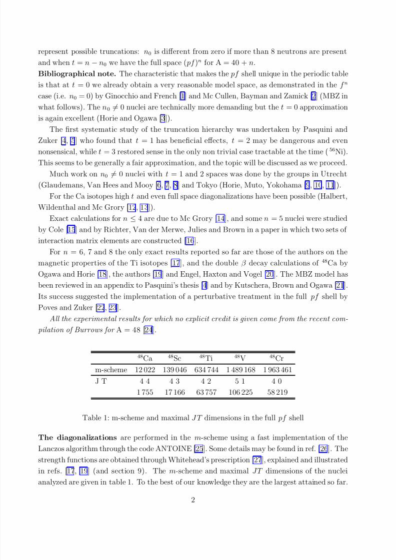
48Ca 48Sc 48Ti 48V 48Cr

m-scheme 12 022 139 046 634 744 1 489 168 1 963 461

J T 4 4 4 3 4 2 5 1 4 0

1 755 17 166 63 757 106 225 58 219

Table 1: m-scheme and maximal J T dimensions in the full pf shell

The diagonalizations are performed in the m-scheme using a fast implementation of the

Lanczos algorithm through the code ANTOINE [25]. Some details may be found in ref. [26]. The

strength functions are obtained through Whitehead’s prescription [27], explained and illustrated

in refs. [17, 19] (and section 9). The m-scheme and maximal JT dimensions of the nuclei

analyzed are given in table 1. To the best of our knowledge they are the largest attained so far.

2

7/25/2019 FIRAS (463)


2 The Interaction and other Operators

The most interesting result of refs. [4, 5] was that the spectroscopic catastrophes generated by

the Kuo-Brown interaction [28] in some nuclei, could be cured by the simple modification (KB’

in [4, 5]).

V T fr(KB1) = V T fr(KB) − (−)T 300 keV (2)

where V T fr are the centroids, defined for any two shells by

V T ij =

J (2J + 1)W JT ijijJ (2J + 1)

, (3)

where the sums run over Pauli allowed values if i = j , and W JT ijij are two body matrix elements.

For i, j ≡ r , no defects can be detected until much higher in the pf region. On the contrary,

the calculations are quite sensitive to changes in W JT

ffff but the only ones that are compulsoryaffect the centroids and it is the binding energies that are sensitive to them:

V 0ff (KB1) = V 0ff (KB)− 350 keV

V 1ff (KB1) = V 1ff (KB)− 110 keV . (4)

The interaction we use in the paper, KB3, was defined in ref. [23] as

W J 0ffff (KB3) = W J 0ffff (KB1) − 300 keV for J = 1, 3

W 21ffff (KB3) = W 21ffff (KB1) − 200 keV. (5)

while the other matrix elements are modified so as to keep the centroids (4).

It should be understood that the minimal interaction is KB1 in that the bad behaviour of

the centroids reflects the bad saturation properties of the realistic potentials: if we do not accept

corrections to the centroids we have no realistic interaction. Compared with the statements

in eqs. (2) and (4), eq. (5) is very small talk that could just as well be ignored. However, to

indulge in it is of some interest, as will become apparent in section 10.

In what follows, and unless specified otherwise, we use

• harmonic oscillator wave functions with b = 1.93fm

• bare electromagnetic factors in M 1 transitions; effective charges of 1.5 e for protons and

0.5 e for neutrons in the electric quadrupole transitions and moments.

• Gamow-Teller (GT) strength defined through

B(GT ) = κ2στ 2, στ = f ||k σktk

±||i√

2J i + 1 , (6)

3

7/25/2019 FIRAS (463)


where the matrix element is reduced with respect to the spin operator only (Racah con-

vention [29]) and κ is the axial to vector ratio for GT decays.

κ = (gA/gV )eff = 0.77(gA/gV )bare = 0.963(7). (7)

• for the Fermi decays we have

B(F ) = τ 2, τ = f ||k tk±||i√

2J i + 1 (8)

• half-lives, t, are found through

(f A + f ǫ)t = 6170± 4

(f V /f A)B(F ) + B(GT ) (9)

We follow ref. [30] in the calculation of the f A and f V integrals and ref. [31] for f ǫ. The

experimental energies are used.

3 48Ca ERRATUM

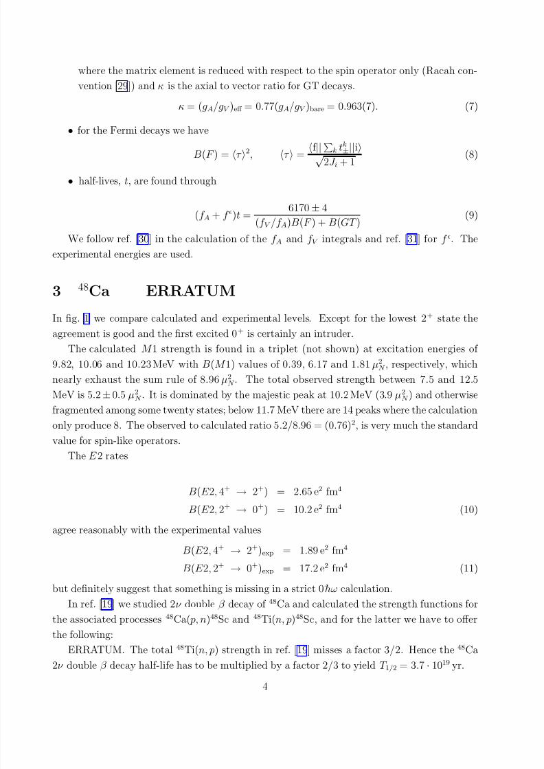
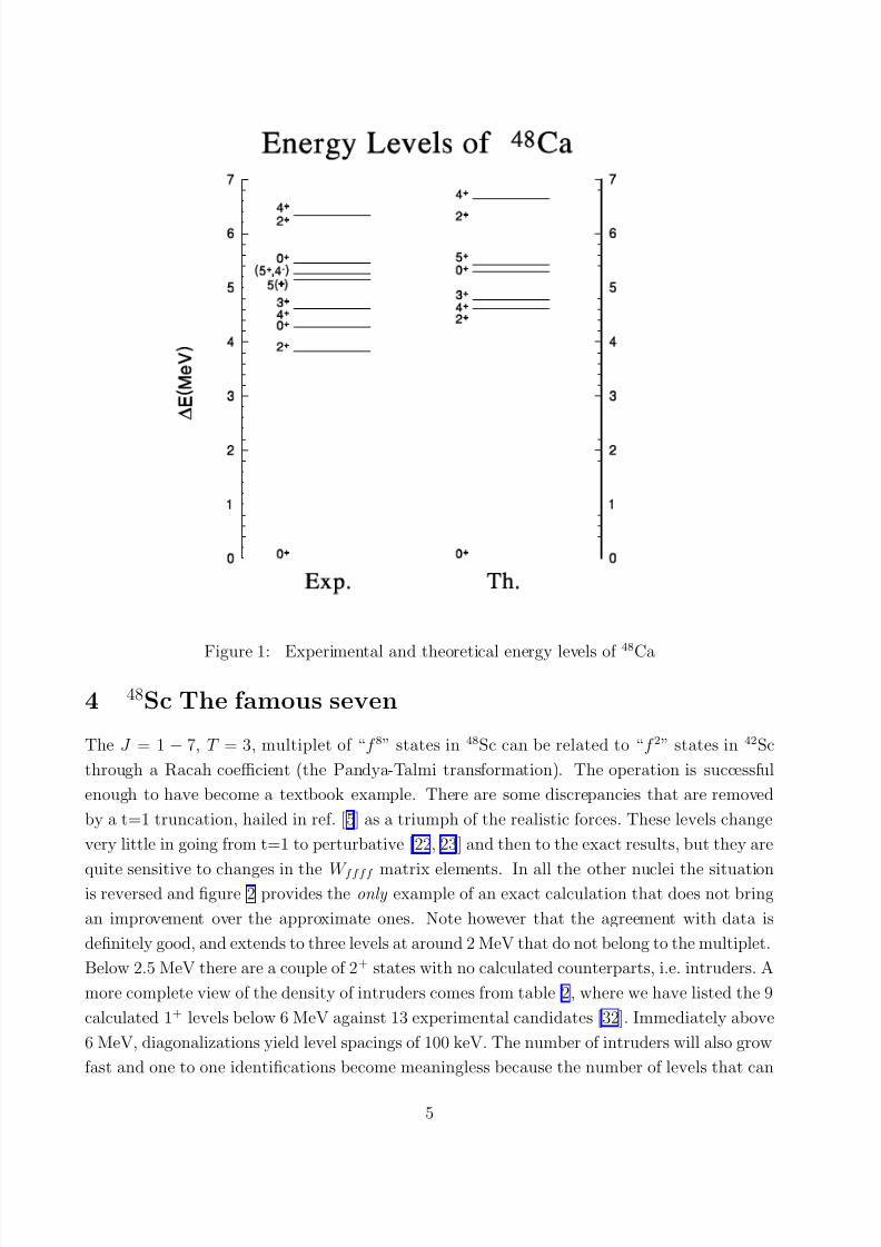
In fig. 1 we compare calculated and experimental levels. Except for the lowest 2+ state the

agreement is good and the first excited 0+ is certainly an intruder.

The calculated M 1 strength is found in a triplet (not shown) at excitation energies of

9.82, 10.06 and 10.23 MeV with B(M 1) values of 0.39, 6.17 and 1.81 µ2N , respectively, which

nearly exhaust the sum rule of 8.96 µ2N . The total observed strength between 7.5 and 12.5

MeV is 5.2

±0.5 µ2N . It is dominated by the majestic peak at 10.2 MeV (3.9 µ2

N ) and otherwise

fragmented among some twenty states; below 11.7 MeV there are 14 peaks where the calculation

only produce 8. The observed to calculated ratio 5.2/8.96 = (0.76)2, is very much the standard

value for spin-like operators.

The E 2 rates

B(E 2, 4+ → 2+) = 2.65 e2 fm4

B(E 2, 2+ → 0+) = 10.2 e2 fm4 (10)

agree reasonably with the experimental values

B(E 2, 4+ → 2+)exp = 1.89 e2 fm4

B(E 2, 2+ → 0+)exp = 17.2 e2 fm4 (11)

but definitely suggest that something is missing in a strict 0 hω calculation.

In ref. [19] we studied 2ν double β decay of 48Ca and calculated the strength functions for

the associated processes 48Ca( p, n)48Sc and 48Ti(n, p)48Sc, and for the latter we have to offer

the following:

ERRATUM. The total 48Ti(n, p) strength in ref. [19] misses a factor 3/2. Hence the 48Ca

2ν double β decay half-life has to be multiplied by a factor 2/3 to yield T 1/2 = 3.7·

1019 yr.

4

7/25/2019 FIRAS (463)


Figure 1: Experimental and theoretical energy levels of 48

Ca

4 48Sc The famous seven

The J = 1 − 7, T = 3, multiplet of “f 8” states in 48Sc can be related to “f 2” states in 42Sc

through a Racah coefficient (the Pandya-Talmi transformation). The operation is successful

enough to have become a textbook example. There are some discrepancies that are removed

by a t=1 truncation, hailed in ref. [5] as a triumph of the realistic forces. These levels change

very little in going from t=1 to perturbative [22, 23] and then to the exact results, but they are

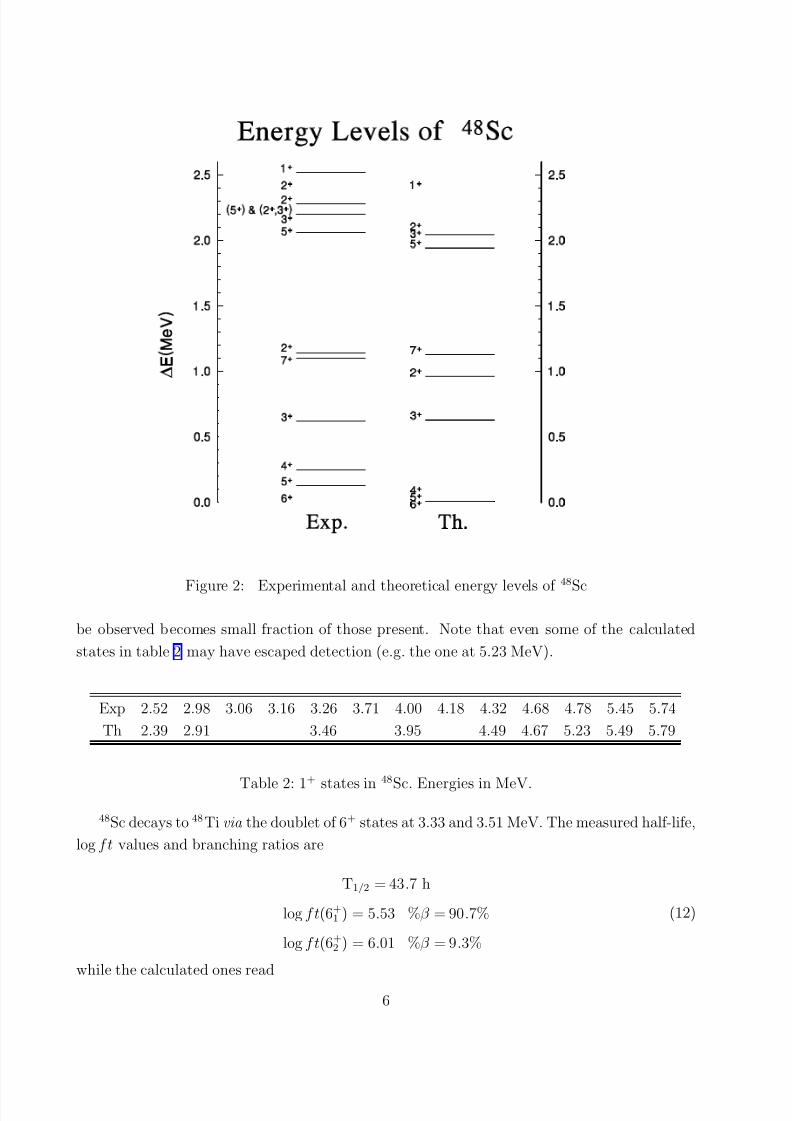
quite sensitive to changes in the W ffff matrix elements. In all the other nuclei the situationis reversed and figure 2 provides the only example of an exact calculation that does not bring

an improvement over the approximate ones. Note however that the agreement with data is

definitely good, and extends to three levels at around 2 MeV that do not belong to the multiplet.

Below 2.5 MeV there are a couple of 2+ states with no calculated counterparts, i.e. intruders. A

more complete view of the density of intruders comes from table 2, where we have listed the 9

calculated 1+ levels below 6 MeV against 13 experimental candidates [32]. Immediately above

6 MeV, diagonalizations yield level spacings of 100 keV. The number of intruders will also grow

fast and one to one identifications become meaningless because the number of levels that can

5

7/25/2019 FIRAS (463)


Figure 2: Experimental and theoretical energy levels of 48

Sc

be observed becomes small fraction of those present. Note that even some of the calculated

states in table 2 may have escaped detection (e.g. the one at 5.23 MeV).

Exp 2.52 2.98 3.06 3.16 3.26 3.71 4.00 4.18 4.32 4.68 4.78 5.45 5.74

Th 2.39 2.91 3.46 3.95 4.49 4.67 5.23 5.49 5.79

Table 2: 1+

states in 48

Sc. Energies in MeV.

48Sc decays to 48Ti via the doublet of 6+ states at 3.33 and 3.51 MeV. The measured half-life,

log f t values and branching ratios are

T1/2 = 43.7 h

log f t(6+1 ) = 5.53 %β = 90.7%

log f t(6+2 ) = 6.01 %β = 9.3%

(12)

while the calculated ones read

6

7/25/2019 FIRAS (463)


T1/2 = 29.14 h

log f t(6+1 ) = 5.34 %β = 96%

log f t(6+2 ) = 6.09 %β = 4%

(13)

We have here a first example of the extreme sensitivity of the half-lives to effects that are

bound to produce very minor changes in other properties that are satisfactorily described, such

as those of the 6+ doublet (see next section).

5 48Ti Intrinsic states

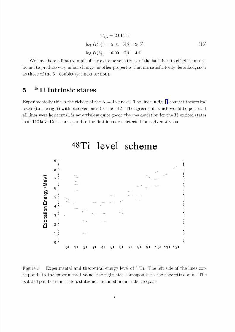
Experimentally this is the richest of the A = 48 nuclei. The lines in fig. 3 connect theoretical

levels (to the right) with observed ones (to the left). The agreement, which would be perfect if

all lines were horizontal, is nevertheless quite good: the rms deviation for the 33 excited statesis of 110 keV. Dots correspond to the first intruders detected for a given J value.

Figure 3: Experimental and theoretical energy level of 48Ti. The left side of the lines cor-

responds to the experimental value, the right side corresponds to the theoretical one. The

isolated points are intruders states not included in our valence space

7

7/25/2019 FIRAS (463)


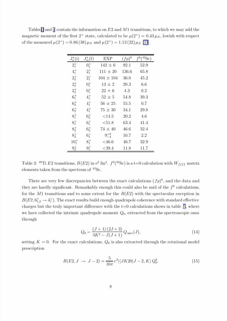
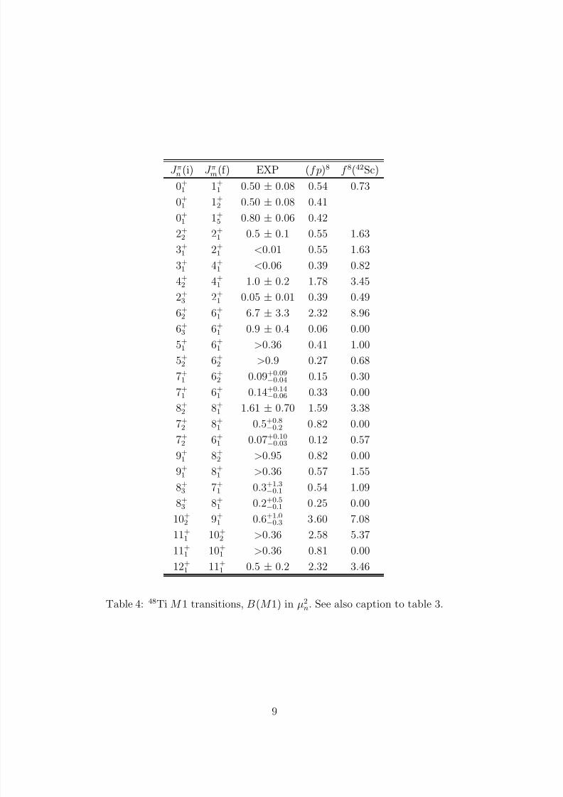
Tables 3 and 4 contain the information on E 2 and M 1 transitions, to which we may add the

magnetic moment of the first 2+ state, calculated to be µ(2+) = 0.43 µN , lowish with respect

of the measured µ(2+) = 0.86 (38) µN and µ(2+) = 1.12 (22) µN [33].

J πn (i) J πm(f) EXP (f p)8 f 8(42Sc)

2+1 0+

1 142 ± 6 92.1 52.9

4+1 2+

1 111 ± 20 136.6 65.8

2+2 2+

1 104 ± 104 36.0 45.2

2+2 0+

1 13 ± 2 20.3 6.6

2+3 0+

1 22 ± 6 4.3 0.2

6+1 4+

1 52 ± 5 54.8 39.3

6+2 4+

1 56 ± 25 55.5 0.7

6+

3 4+

1 75

± 30 34.1 29.8

8+1 6+

2 <14.5 20.2 4.6

8+1 6+

1 <51.8 63.4 41.4

8+2 6+

2 74 ± 40 46.6 32.4

8+2 6+

1 9+9−4 10.7 2.2

10+1 8+

1 <46.6 46.7 32.9

9+2 9+

1 <39.4 11.8 11.7

Table 3: 48Ti E 2 transitions, B(E 2) in e2 fm4. f 8(42Sc) is a t=0 calculation with W ffff matrix

elements taken from the spectrum of 42Sc.

There are very few discrepancies between the exact calculations (f p)8, and the data and

they are hardly significant. Remarkably enough this could also be said of the f 8 calculations,

for the M 1 transitions and to some extent for the B(E 2) with the spectacular exception in

B(E 2, 6+1,2 → 4+

1 ). The exact results build enough quadrupole coherence with standard effective

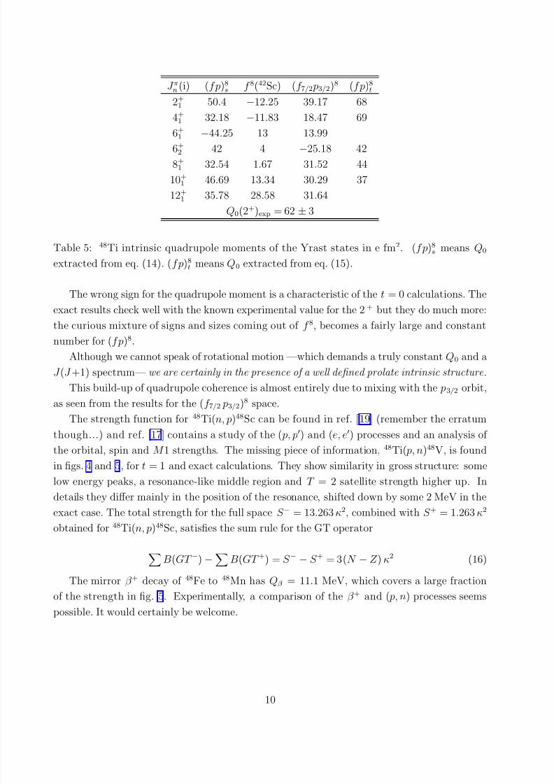
charges but the truly important difference with the t=0 calculations shows in table 5, where

we have collected the intrinsic quadrupole moment Q0, extracted from the spectroscopic ones

through

Q0 = (J + 1) (2J + 3)

3K 2 − J (J + 1) Qspec(J ), (14)

setting K = 0. For the exact calculations, Q0 is also extracted through the rotational model

prescription

B(E 2, J → J − 2) = 5

16π e2|JK 20|J − 2, K Q2

0. (15)

8

7/25/2019 FIRAS (463)


J πn (i) J πm(f) EXP (f p)8 f 8(42Sc)

0+1 1+

1 0.50 ± 0.08 0.54 0.73

0+1 1+

2 0.50 ± 0.08 0.41

0+1 1+

5 0.80 ± 0.06 0.42

2+2 2+

1 0.5 ± 0.1 0.55 1.63

3+1 2+

1 <0.01 0.55 1.63

3+1 4+

1 <0.06 0.39 0.82

4+2 4+1 1.0 ± 0.2 1.78 3.452+3 2+

1 0.05 ± 0.01 0.39 0.49

6+2 6+

1 6.7 ± 3.3 2.32 8.96

6+3 6+

1 0.9 ± 0.4 0.06 0.00

5+1 6+

1 >0.36 0.41 1.00

5+2 6+

2 >0.9 0.27 0.68

7+1 6+

2 0.09+0.09−0.04 0.15 0.30

7+1 6+

1 0.14+0.14−0.06 0.33 0.00

8+2 8+

1 1.61

± 0.70 1.59 3.38

7+2 8+

1 0.5+0.8−0.2 0.82 0.00

7+2 6+

1 0.07+0.10−0.03 0.12 0.57

9+1 8+

2 >0.95 0.82 0.00

9+1 8+

1 >0.36 0.57 1.55

8+3 7+

1 0.3+1.3−0.1 0.54 1.09

8+3 8+

1 0.2+0.5−0.1 0.25 0.00

10+2 9+

1 0.6+1.0−0.3 3.60 7.08

11+1 10+

2 >0.36 2.58 5.37

11+1 10+

1 >0.36 0.81 0.00

12+1 11+

1 0.5 ± 0.2 2.32 3.46

Table 4: 48Ti M 1 transitions, B(M 1) in µ2n. See also caption to table 3.

9

7/25/2019 FIRAS (463)


J πn (i) (f p)8s f 8(42Sc) (f 7/2 p3/2)8 (f p)8t2+1 50.4 −12.25 39.17 68

4+1 32.18 −11.83 18.47 69

6+

1 −44.25 13 13.996+2 42 4 −25.18 42

8+1 32.54 1.67 31.52 44

10+1 46.69 13.34 30.29 37

12+1 35.78 28.58 31.64

Q0(2+)exp = 62 ± 3

Table 5: 48Ti intrinsic quadrupole moments of the Yrast states in e fm2. (f p)8s means Q0

extracted from eq. (14). (f p)8t means Q0 extracted from eq. (15).

The wrong sign for the quadrupole moment is a characteristic of the t = 0 calculations. The

exact results check well with the known experimental value for the 2+ but they do much more:

the curious mixture of signs and sizes coming out of f 8, becomes a fairly large and constant

number for (f p)8.

Although we cannot speak of rotational motion —which demands a truly constant Q0 and a

J (J +1) spectrum— we are certainly in the presence of a well defined prolate intrinsic structure .

This build-up of quadrupole coherence is almost entirely due to mixing with the p3/2 orbit,

as seen from the results for the (f 7/2 p3/2)8 space.

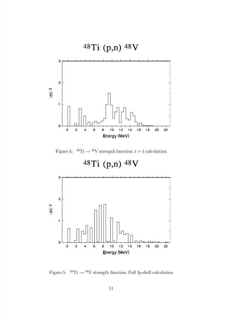
The strength function for 48Ti(n, p)48Sc can be found in ref. [19] (remember the erratum

though...) and ref. [17] contains a study of the ( p, p′) and (e, e′) processes and an analysis of

the orbital, spin and M 1 strengths. The missing piece of information, 48Ti( p, n)48V, is found

in figs. 4 and 5, for t = 1 and exact calculations. They show similarity in gross structure: some

low energy peaks, a resonance-like middle region and T = 2 satellite strength higher up. In

details they differ mainly in the position of the resonance, shifted down by some 2 MeV in the

exact case. The total strength for the full space S − = 13.263 κ2, combined with S + = 1.263 κ2

obtained for 48Ti(n, p)48Sc, satisfies the sum rule for the GT operator

B(GT −) −B(GT +) = S − − S + = 3(N − Z ) κ2 (16)

The mirror β + decay of 48Fe to 48Mn has Qβ = 11.1 MeV, which covers a large fraction

of the strength in fig. 5. Experimentally, a comparison of the β + and ( p, n) processes seems

possible. It would certainly be welcome.

10

7/25/2019 FIRAS (463)


Figure 4: 48Ti → 48V strength function. t = 1 calculation

Figure 5: 48Ti → 48V strength function. Full fp-shell calculation

11

7/25/2019 FIRAS (463)


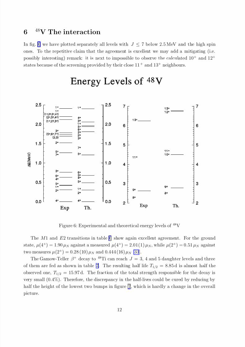
6 48V The interaction

In fig. 6 we have plotted separately all levels with J ≤ 7 below 2.5 MeV and the high spin

ones. To the repetitive claim that the agreement is excellent we may add a mitigating (i.e.

possibly interesting) remark: it is next to impossible to observe the calculated 10+ and 12+

states because of the screening provided by their close 11+ and 13+ neighbours.

Figure 6: Experimental and theoretical energy levels of 48V

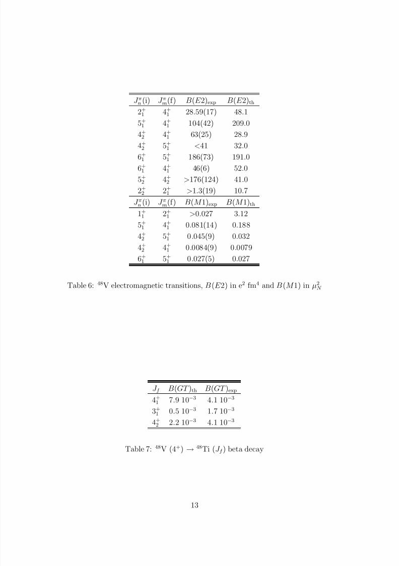
The M 1 and E 2 transitions in table 6 show again excellent agreement. For the ground

state, µ(4+) = 1.90 µN against a measured µ(4+) = 2.01(1) µN , while µ(2+) = 0.51 µN against

two measures µ(2+) = 0.28 (10) µN and 0.444 (16) µN [33].

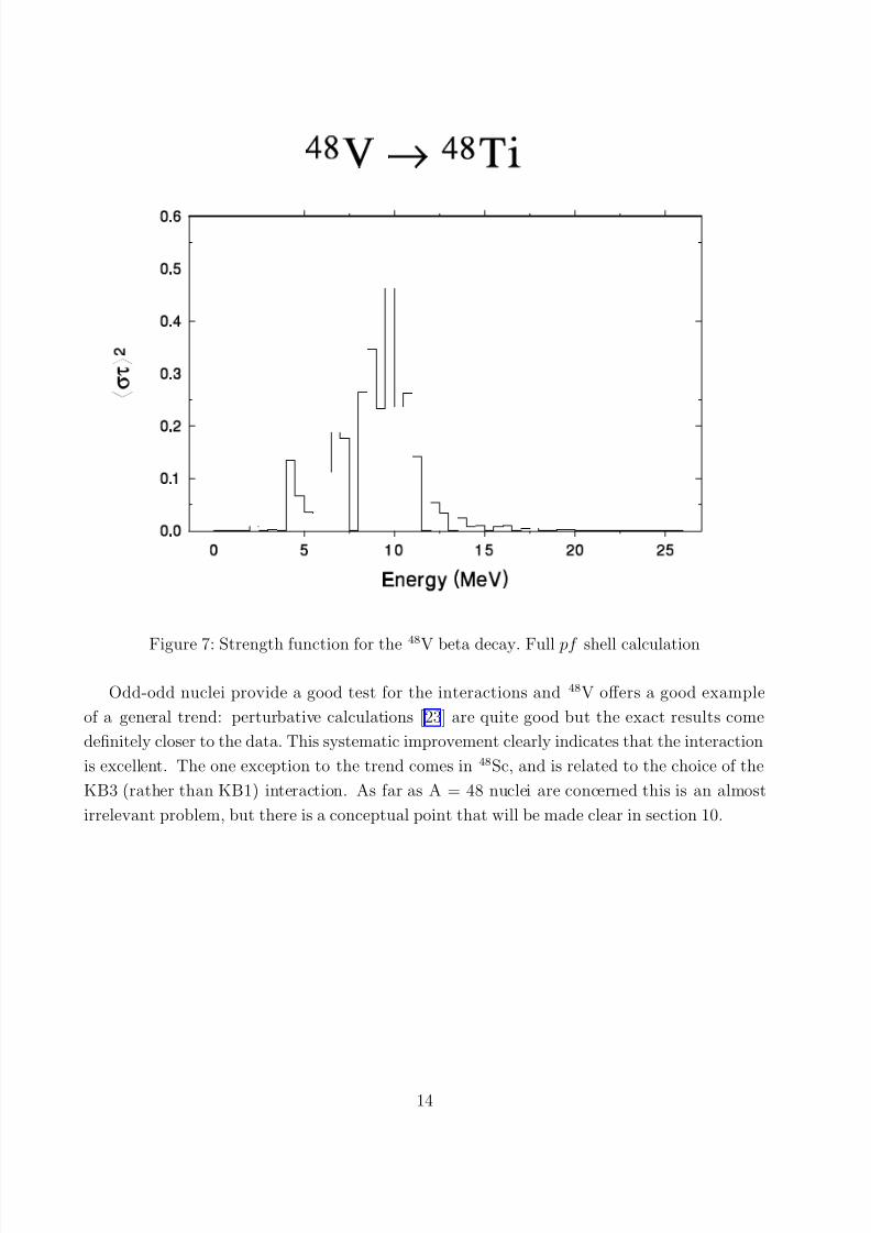
The Gamow-Teller β + decay to 48Ti can reach J = 3, 4 and 5 daughter levels and three

of them are fed as shown in table 7. The resulting half life T 1/2 = 8.85 d is almost half the

observed one, T 1/2 = 15.97 d. The fraction of the total strength responsible for the decay is

very small (0.4%). Therefore, the discrepancy in the half-lives could be cured by reducing by

half the height of the lowest two bumps in figure 7, which is hardly a change in the overall

picture.

12

7/25/2019 FIRAS (463)


J πn (i) J πm(f) B(E 2)exp B(E 2)th

2+1 4+

1 28.59(17) 48.1

5+1 4+

1 104(42) 209.0

4+2 4+

1 63(25) 28.9

4+2 5+

1 <41 32.0

6+1 5+

1 186(73) 191.0

6+1 4+

1 46(6) 52.0

5+2 4+

2 >176(124) 41.0

2+2 2+

1 >1.3(19) 10.7

J πn (i) J πm(f) B(M 1)exp B(M 1)th

1+1 2+

1 >0.027 3.12

5+1 4+

1 0.081(14) 0.188

4+2 5+

1 0.045(9) 0.032

4+2 4+

1 0.0084(9) 0.0079

6+1 5+

1 0.027(5) 0.027

Table 6: 48V electromagnetic transitions, B(E 2) in e2 fm4 and B(M 1) in µ2N

J f B(GT )th B(GT )exp

4+1 7.9 10−3 4.1 10−3

3+1 0.5 10−3 1.7 10−3

4+2 2.2 10−3 4.1 10−3

Table 7: 48V (4+) → 48Ti (J f ) beta decay

13

7/25/2019 FIRAS (463)


Figure 7: Strength function for the 48

V beta decay. Full pf shell calculation

Odd-odd nuclei provide a good test for the interactions and 48V offers a good example

of a general trend: perturbative calculations [23] are quite good but the exact results come

definitely closer to the data. This systematic improvement clearly indicates that the interaction

is excellent. The one exception to the trend comes in 48Sc, and is related to the choice of the

KB3 (rather than KB1) interaction. As far as A = 48 nuclei are concerned this is an almost

irrelevant problem, but there is a conceptual point that will be made clear in section 10.

14

7/25/2019 FIRAS (463)


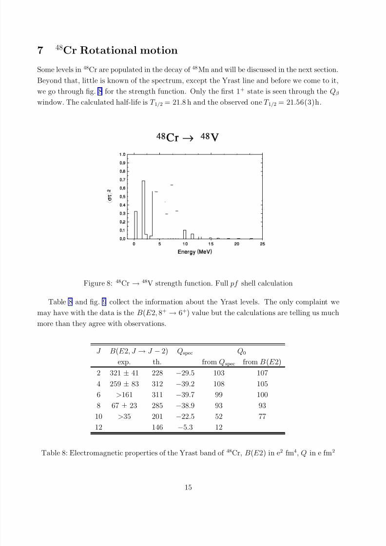
7 48Cr Rotational motion

Some levels in 48Cr are populated in the decay of 48Mn and will be discussed in the next section.

Beyond that, little is known of the spectrum, except the Yrast line and before we come to it,

we go through fig. 8 for the strength function. Only the first 1+ state is seen through the Qβ

window. The calculated half-life is T 1/2 = 21.8 h and the observed one T 1/2 = 21.56(3)h.

Figure 8:

48

Cr → 48

V strength function. Full pf shell calculation

Table 8 and fig. 9 collect the information about the Yrast levels. The only complaint we

may have with the data is the B(E 2, 8+ → 6+) value but the calculations are telling us much

more than they agree with observations.

J B(E 2, J → J − 2) Qspec Q0

exp. th. from Qspec from B(E 2)

2 321 ± 41 228 −29.5 103 107

4 259 ± 83 312 −39.2 108 1056 >161 311 −39.7 99 100

8 67 ± 23 285 −38.9 93 93

10 >35 201 −22.5 52 77

12 146 −5.3 12

Table 8: Electromagnetic properties of the Yrast band of 48Cr, B(E 2) in e2 fm4, Q in e fm2

15

7/25/2019 FIRAS (463)


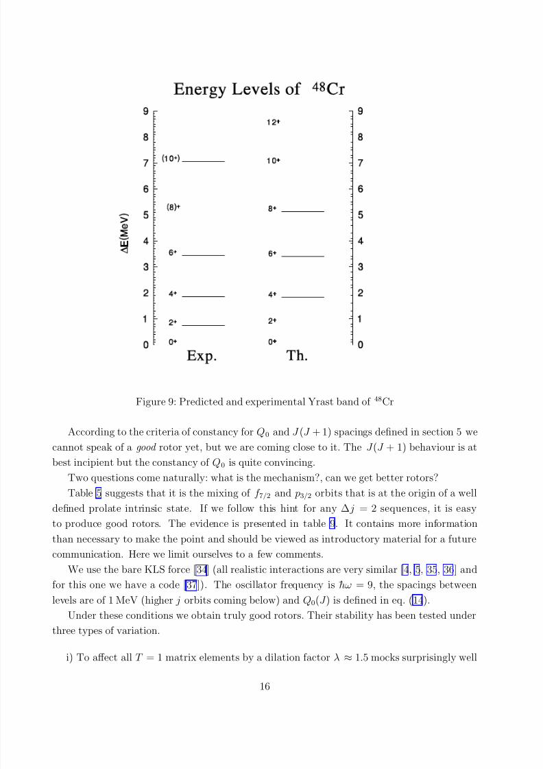
Figure 9: Predicted and experimental Yrast band of 48

Cr

According to the criteria of constancy for Q0 and J (J + 1) spacings defined in section 5 we

cannot speak of a good rotor yet, but we are coming close to it. The J (J + 1) behaviour is at

best incipient but the constancy of Q0 is quite convincing.

Two questions come naturally: what is the mechanism?, can we get better rotors?

Table 5 suggests that it is the mixing of f 7/2 and p3/2 orbits that is at the origin of a well

defined prolate intrinsic state. If we follow this hint for any ∆ j = 2 sequences, it is easy

to produce good rotors. The evidence is presented in table 9. It contains more information

than necessary to make the point and should be viewed as introductory material for a futurecommunication. Here we limit ourselves to a few comments.

We use the bare KLS force [34] (all realistic interactions are very similar [4, 5, 35, 36] and

for this one we have a code [37]). The oscillator frequency is hω = 9, the spacings between

levels are of 1 MeV (higher j orbits coming below) and Q0(J ) is defined in eq. (14).

Under these conditions we obtain truly good rotors. Their stability has been tested under

three types of variation.

i) To affect all T = 1 matrix elements by a dilation factor λ ≈ 1.5 mocks surprisingly well

16

7/25/2019 FIRAS (463)


core polarization effects in a major shell [35, 36]. Rotational behaviour persists and may

be even emphasized.

ii) For splittings between levels of 2 MeV the rotational features are eroded but E 4/E 2 > 3

in all cases.

iii) Pairing is the most efficient enemy of good rotors. To go from KLS (bare) to KB (renor-

malized), λ = 1.5) (from i)) is sufficient, except for W 01ffff which should be doubled. Then

E 4/E 2 ≈ 2.5, not far from what is seen in fig. 9.

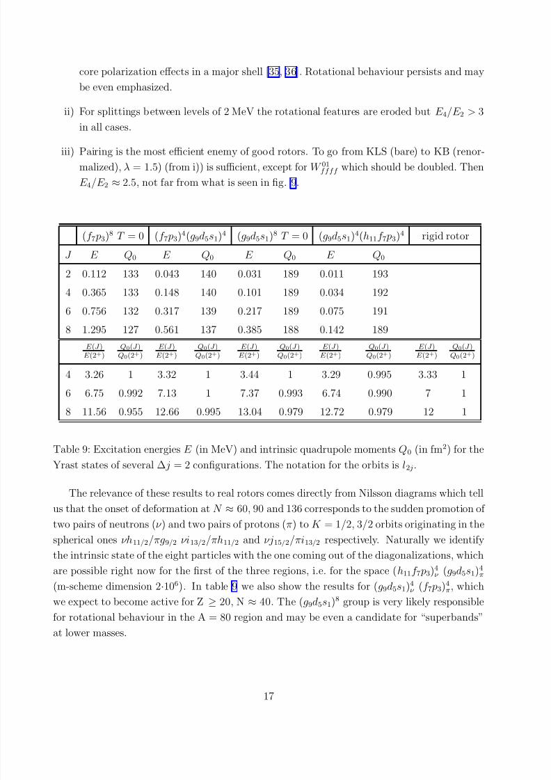
(f 7 p3)8 T = 0 (f 7 p3)4(g9d5s1)4 (g9d5s1)8 T = 0 (g9d5s1)4(h11f 7 p3)4 rigid rotor

J E Q0 E Q0 E Q0 E Q0

2 0.112 133 0.043 140 0.031 189 0.011 193

4 0.365 133 0.148 140 0.101 189 0.034 192

6 0.756 132 0.317 139 0.217 189 0.075 191

8 1.295 127 0.561 137 0.385 188 0.142 189

E (J )E (2+)

Q0(J )Q0(2+)

E (J )E (2+)

Q0(J )Q0(2+)

E (J )E (2+)

Q0(J )Q0(2+)

E (J )E (2+)

Q0(J )Q0(2+)

E (J )E (2+)

Q0(J )Q0(2+)

4 3.26 1 3.32 1 3.44 1 3.29 0.995 3.33 1

6 6.75 0.992 7.13 1 7.37 0.993 6.74 0.990 7 1

8 11.56 0.955 12.66 0.995 13.04 0.979 12.72 0.979 12 1

Table 9: Excitation energies E (in MeV) and intrinsic quadrupole moments Q0 (in fm2) for the

Yrast states of several ∆ j = 2 configurations. The notation for the orbits is l2 j.

The relevance of these results to real rotors comes directly from Nilsson diagrams which tell

us that the onset of deformation at N ≈ 60, 90 and 136 corresponds to the sudden promotion of

two pairs of neutrons (ν ) and two pairs of protons (π) to K = 1/2, 3/2 orbits originating in the

spherical ones νh11/2/πg9/2 νi13/2/πh11/2 and νj15/2/πi13/2 respectively. Naturally we identify

the intrinsic state of the eight particles with the one coming out of the diagonalizations, which

are possible right now for the first of the three regions, i.e. for the space (h11f 7 p3)4ν (g9d5s1)4π(m-scheme dimension 2·106). In table 9 we also show the results for (g9d5s1)4ν (f 7 p3)4π, which

we expect to become active for Z ≥ 20, N ≈ 40. The (g9d5s1)8 group is very likely responsible

for rotational behaviour in the A = 80 region and may be even a candidate for “superbands”

at lower masses.

17

7/25/2019 FIRAS (463)


8 48Mn Truncations and GT strength

Spectroscopically, 48Mn is identical to 48V (to within Coulomb effects). Its decay to 48Cr covers

a non negligible fraction of the strength function [38, 39]. Since this process, and similar ones

in the region, have been analyzed so far with t = 1 calculations, we are going to compare them

with t = 3 and exact ones. A digression may be of use.

In a decay, the parent is basically an f n state. Some daughters are also of f n type but most

are f n−1r. In a t = 1 calculation, both configurations are present but f n is allowed to mix with

f n−1r through W fffr matrix elements while f n−1r is not allowed to go to f n−2r2. At the t = 2

level, pairing (i.e. W ffrr matrix elements) comes in and pushes f n down through mixing with

f n−2r2, while f n−1r cannot benefit from a similar push from f n−3r3. It is only at the t = 3 level

that both f n and f n−1r states can be treated on equal footing. Now that t = 3 calculations

are possible up to A = 58, it is useful to check their validity.

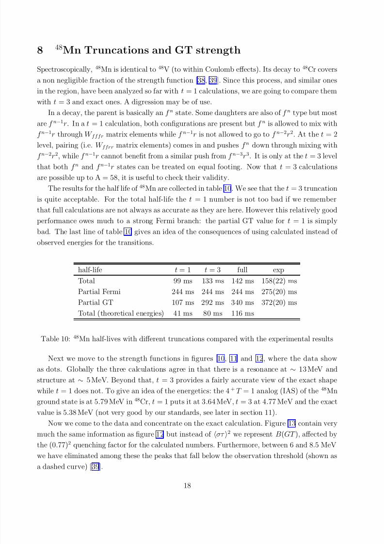
The results for the half life of 48

Mn are collected in table 10. We see that the t = 3 truncationis quite acceptable. For the total half-life the t = 1 number is not too bad if we remember

that full calculations are not always as accurate as they are here. However this relatively good

performance owes much to a strong Fermi branch: the partial GT value for t = 1 is simply

bad. The last line of table 10 gives an idea of the consequences of using calculated instead of

observed energies for the transitions.

half-life t = 1 t = 3 full exp

Total 99 ms 133 ms 142 ms 158(22) ms

Partial Fermi 244 ms 244 ms 244 ms 275(20) ms

Partial GT 107 ms 292 ms 340 ms 372(20) ms

Total (theoretical energies) 41 ms 80 ms 116 ms

Table 10: 48Mn half-lives with different truncations compared with the experimental results

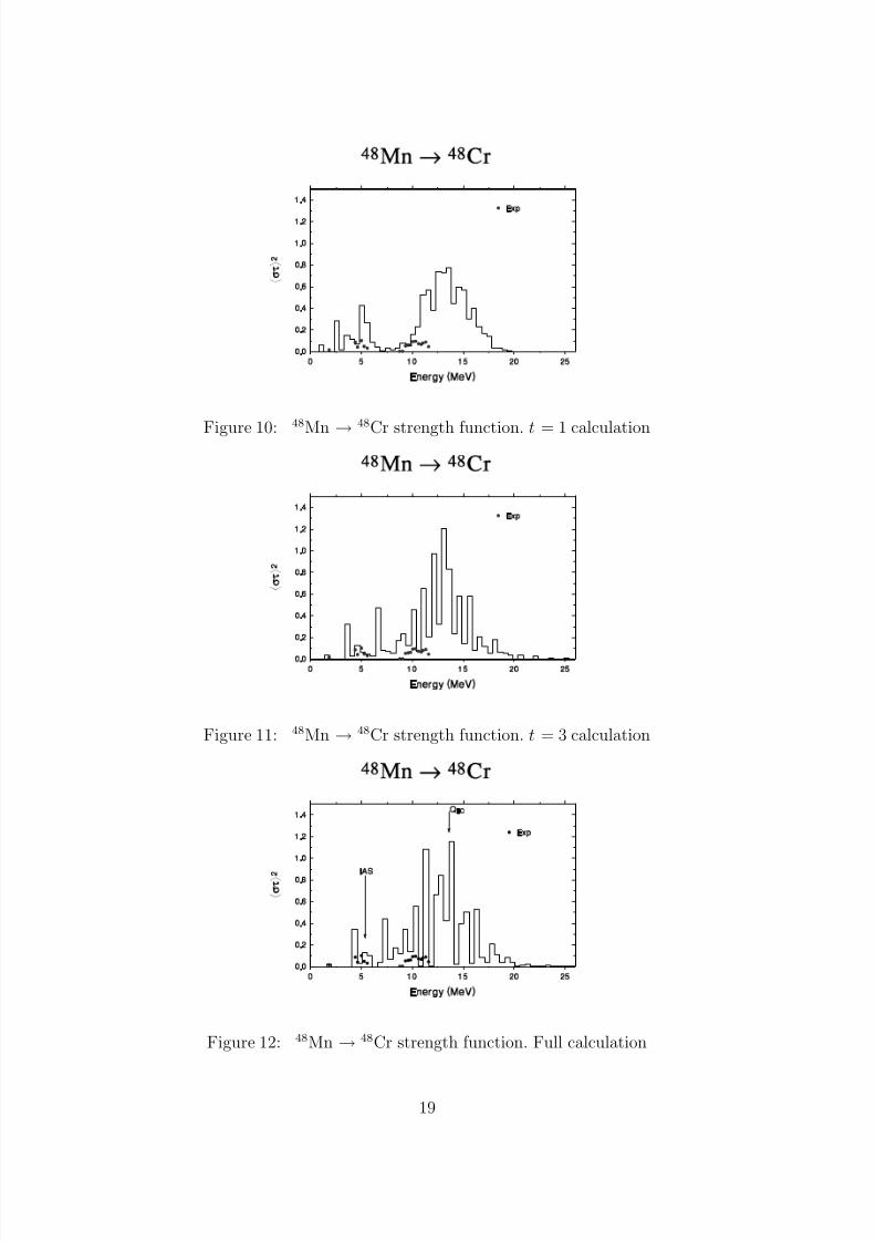
Next we move to the strength functions in figures 10, 11 and 12, where the data show

as dots. Globally the three calculations agree in that there is a resonance at ∼ 13 MeV and

structure at ∼ 5 MeV. Beyond that, t = 3 provides a fairly accurate view of the exact shapewhile t = 1 does not. To give an idea of the energetics: the 4+ T = 1 analog (IAS) of the 48Mn

ground state is at 5.79 MeV in 48Cr, t = 1 puts it at 3.64 MeV, t = 3 at 4.77 MeV and the exact

value is 5.38 MeV (not very good by our standards, see later in section 11).

Now we come to the data and concentrate on the exact calculation. Figure 13 contain very

much the same information as figure 12 but instead of στ 2 we represent B(GT ), affected by

the (0.77)2 quenching factor for the calculated numbers. Furthermore, between 6 and 8.5 MeV

we have eliminated among these the peaks that fall below the observation threshold (shown as

a dashed curve) [39].

18

7/25/2019 FIRAS (463)


Figure 10: 48

Mn → 48

Cr strength function. t = 1 calculation

Figure 11: 48Mn → 48Cr strength function. t = 3 calculation

Figure 12: 48Mn → 48Cr strength function. Full calculation

19

7/25/2019 FIRAS (463)


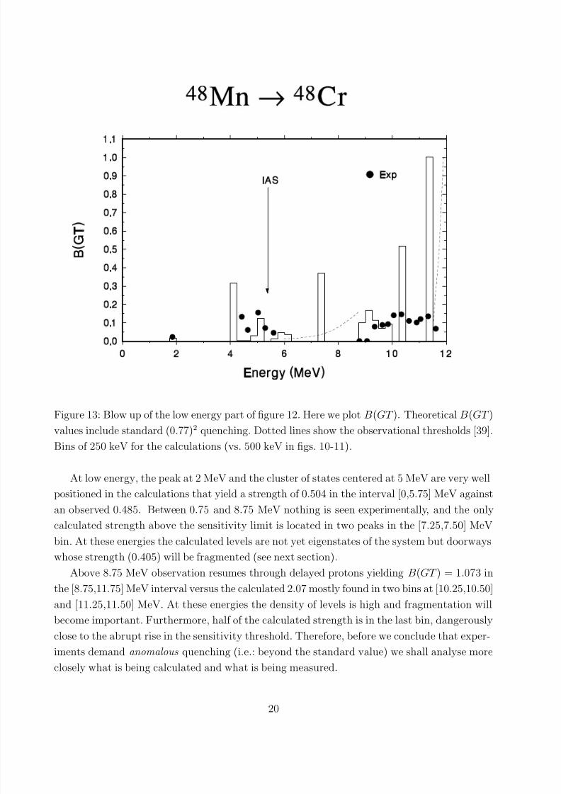
Figure 13: Blow up of the low energy part of figure 12. Here we plot B(GT ). Theoretical B(GT )values include standard (0.77)2 quenching. Dotted lines show the observational thresholds [39].

Bins of 250 keV for the calculations (vs. 500 keV in figs. 10-11).

At low energy, the peak at 2 MeV and the cluster of states centered at 5 MeV are very well

positioned in the calculations that yield a strength of 0.504 in the interval [0,5.75] MeV against

an observed 0.485. Between 0.75 and 8.75 MeV nothing is seen experimentally, and the only

calculated strength above the sensitivity limit is located in two peaks in the [7.25,7.50] MeV

bin. At these energies the calculated levels are not yet eigenstates of the system but doorways

whose strength (0.405) will be fragmented (see next section).Above 8.75 MeV observation resumes through delayed protons yielding B(GT ) = 1.073 in

the [8.75,11.75] MeV interval versus the calculated 2.07 mostly found in two bins at [10.25,10.50]

and [11.25,11.50] MeV. At these energies the density of levels is high and fragmentation will

become important. Furthermore, half of the calculated strength is in the last bin, dangerously

close to the abrupt rise in the sensitivity threshold. Therefore, before we conclude that exper-

iments demand anomalous quenching (i.e.: beyond the standard value) we shall analyse more

closely what is being calculated and what is being measured.

20

7/25/2019 FIRAS (463)


9 Quenching, shifting and diluting GT strength

From all we have said about GT transitions, a broad trend emerges: low lying levels are very

well positioned and within minor discrepancies have the observed GT strength once standard

quenching is applied. The examples of good energetics are particularly significant for the group

around 5 MeV in 48Cr and the 1+ levels in 48Ti (fig. 3) and 48Sc (table 2), that have experimental

counterparts within 100 keV more often than not. The discrepancies are related to the shortish

half-life of 48Sc and 48V, a slight lack of spin strength in the lowest states of 48Ti (ref. [17]) and

—perhaps— with the tail of the resonant structure in 48Cr discussed in the preceding section.

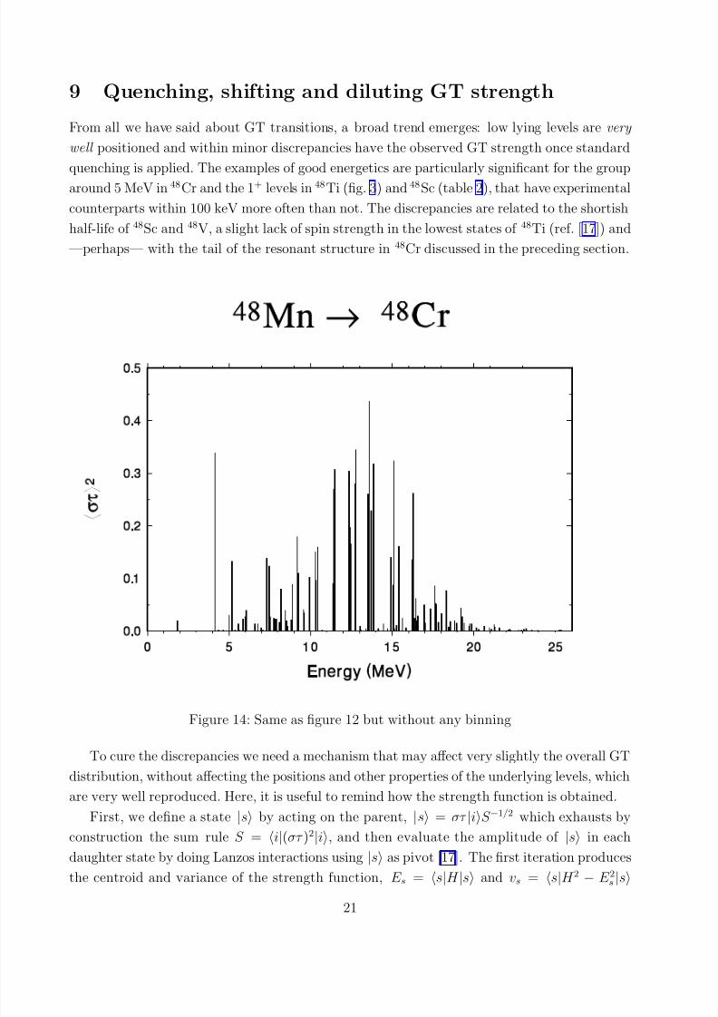
Figure 14: Same as figure 12 but without any binning

To cure the discrepancies we need a mechanism that may affect very slightly the overall GT

distribution, without affecting the positions and other properties of the underlying levels, which

are very well reproduced. Here, it is useful to remind how the strength function is obtained.

First, we define a state |s by acting on the parent, |s = στ |iS −1/2 which exhausts by

construction the sum rule S = i|(στ )2|i, and then evaluate the amplitude of |s in each

daughter state by doing Lanzos interactions using |s as pivot [17]. The first iteration produces

the centroid and variance of the strength function, E s =

s

|H

|s

and vs =

s

|H 2

−E 2s|s

21

7/25/2019 FIRAS (463)


respectively. As the number of iterations ν increases, the strength —originally concentrated at

E s — is fragmented into ν peaks. The lowest converge to exact eigenstates (with their exact

share of the total sum rule) at the rate of roughly one every 6-10 iterations. Figure 14 is the

high resolution version of fig. 12 and shows the situation after 60 iterations for each of the

JT values (J = 3, 4, 5; T = 0, 1, 2). It is only below approximately 6 MeV that we have acomplete picture of the spectrum. Above, many thousand states are waiting to come and erode

the strong peaks.

Let us examine first the global properties associated with S and E s and then turn to the

consequences of local fragmentation.

Quenching. Calculations always produce too much strength, that has to be reduced by a

quenching factor, which is the stronger (i.e. smaller) the most drastic the truncation [17].

For exact calculations in one major shell (0hω), S has to be reduced by (0.77)2, which is

very much the value demanded by the “violation” of the model independent sum rule (16).There is very little we can do within a 0hω calculation to change this state of affairs.

Shifting. Contrary to S , which depends on geometry (16) and on overall properties of H ,

E s may be significantly affected by small changes in the σ · σ and στ · στ contributions

to H . In ref. [36] it is shown that these spin-spin terms are very strong, especially the

second, and may differ from force to force by some 20% (the corresponding constants e1+0

and e1+1 in ref. [36] are related, but not trivially, to the Migdal parameters g and g′).

Therefore, the mechanism to cure the small discrepancies we have mentioned may well

come from modifications in these numbers, that would produce small overall shifts of the

distribution, and nothing else.

Now we return to the quenching problem. In view of discrepancies between ( p, n) and

β + data for 37Ca, the extraction of S from the former has been recently criticized [40, 41].

The problem was compounded by the fact that calculations with Wildenthal’s W interaction

suggested that standard quenching did not seem necessary. This illusion was dispelled by

Brown’s analysis [42], showing that the interaction was at fault. It is very interesting to note

that what is called 12.5p in [42] is none other that KB, while CW —which gives the best

results— is very basically a minimally modified KB that can be safely assimilated to KB1 or

KB3.

Diluting. Brown’s analysis contains another important hint: once normalized by the (0.77)2

factor, the CW calculations follow smoothly the data within the β window, but then

produce too much strength when compared with the ( p, n) reaction. The suggestion from

fig. 14 is that in regions where the density of levels becomes high, fragmentation may be-

come so strong that much strength will be so diluted as to be rendered unobservable. The

difference between the A = 37 and A = 48 spectra is that in the former the effect is almost

exclusively due to intruders, while in the latter the density of pf states is high enough

22

7/25/2019 FIRAS (463)


to produce substantial dilution by itself. Which brings us back to the problem of the

amount of strength calculated between 8.75 and 11.75 MeV in 48Cr, double the measured

value. Some shifting may be warranted to reduce the discrepancy, but fig. 14 suggest very

strongly that dilution be made responsible for it (i.e. for anomalous quenching)

From all this, it follows that simultaneous measurements of β + and ( p, n) strength are very

much welcome in pairs of conjugate nuclei where the β + release energy is large, the 0hω spectrum

is dense and high quality calculations are feasible. We propose the following candidates:

β + ( p, n)45Cr → 45V 45Sc → 45Ti46Cr → 46V 46Ti → 46V

47Mn → 47Cr 47Ti → 47V48Fe

→ 48Mn 48Ti

→ 48V.

To conclude: a theoretical understanding of standard quenching demands that we look

at the full wavefunction and not only at its 0hω components. Experimentally, what has to be

explained is the disappearance of strength, i.e. standard and anomalous quenching (as observed

in 48Cr). Dilution will no doubt play a role in both, but the latter may be observed already by

comparisons with 0hω calculations.

10 The validity of monopole modified realistic interac-

tionsTo answer with some care the question raised in the introduction we review briefly the work

related to monopole corrections.

The first attempt to transpose the results of refs. [4, 5] to the sd shell met with the problem

that the interaction had to evolve from 16O to 40Ca. A linear evolution was assumed, but it

was shown that the centroids followed more complicated laws demanding an excessive number

of parameters [43].

The solution came in ref. [35], by adopting a hierarchy of centroids and noting that the

realistic matrix elements depend on the harmonic oscillator frequency very much as

W JT rstu(ω) = ω

ω0W JT rstu(ω0), (17)

thus displacing the problem of evolution of H to one of evolution of ω. The classical estimate

hω = 40A−1/3 [44] relies on filling oscillator orbits and on adopting the r = r0A1/3 law for radii,

which nuclei in the p and sd shells do not follow. Therefore it was decided to treat ω as a

free parameter for each mass number and then check that the corresponding oscillator orbits

reproduce the observed radii. This turned out to work very well and to produce very good

spectroscopy in all regions where exact calculations could be done.

23

7/25/2019 FIRAS (463)


The method relies on the rigorous decomposition of the full Hamiltonian as H = Hm +

HM , where the monopole part Hm is responsible for saturation properties, while HM contains

all the other multipoles. Upon reduction to a model H,Hm is represented by H m, which

contains the binding energies of the closed shells, the single particle energies and the centroids.

Everything else goes to H M , which nevertheless depends on Hm through the orbits, in principleselfconsistently extracted from Hm [35, 36, 45]. The program of minimal modifications now

amounts to discard from the nucleon-nucleon potential the Hm part and accept all the rest,

unless some irrefutable arguments show up for modifying something else. On the contrary Hmis assumed to be purely phenomenological and the information necessary to construct it comes

mostly from masses and single particle energies [45].

The proof of the validity of the realistic HM through shell model calculations depends on

the quality of the monopole corrections. In regions of agitated radial behaviour we have to

go beyond the oscillator approximation. In particular, the sd shell radii can be reproduced

practically within error bars by Hartree-Fock calculations with Skyrme forces with orbitalfillings extracted from the shell model wave functions [46]. Obviously the d5/2, s1/2 and d3/2

orbits are poorly reproduced by a single ω, and obviously this makes a difference in the two

body matrix elements [34] (work is under progress on this problem).

Therefore, in the sd shell —to match or better the energy agreements obtained with Wilden-

thal’s famous W (or USD) interaction [47, 48]— we have to push a bit further the work of

ref. [35].

When we move to the pf shell, no such efforts are, or were, necessary. Because of f 7/2

dominance, it is much easier to determine the centroids: the V T rr values are no issue, the crucial

V T fr ones can be read (almost) directly from single particle properties on 49Ca and 57Ni, and

we are left with V T ff ; only two numbers. Once we have good enough approximations for the

centroids we can do shell model calculations to see how the rest of H (i.e. H M ) behaves. In

ref. [23] it was found that H M behaves quite well, but much better in the second half of the f n

region: A = 48 happens to be the border beyond which quite well becomes very well. Hence

the remark in the second paragraph of the introduction.

The trouble at the beginning of the region was attributed at the time to intruders, but

now we know that radial behaviour must be granted its share. It is here that KB3 comes in.

Although eq. 5 has only cosmetic effects, its origin is not cosmetic: it was meant to simulate

necessary corrective action not related to the presence of intruders . It reflects the fact that in the

neighborhood of 40Ca the interaction works better if the spectrum of 42Sc is better reproduced,

while at A = 48 and after, the KB interaction —not very good in 42Sc— needs no help, except

in the centroids, as we have shown.

Most probably this says something about radial behaviour at the beginning of the region.

It is poorly known except in the Ca isotopes, where it is highly non trivial [ 49]. The indications

are that when shell model calculations demand individual variations of matrix elements in

going from nucleus to nucleus the most likely culprits are the single particle orbits. And the

24

7/25/2019 FIRAS (463)


indications are that at A = 48 the need for such considerations disappears.

All this is to say that A = 48 happens to be a good place for a test of the interaction and

KB1 passes it with honours. It also amounts to say that it is not an accident but part of the

general statement that monopole corrected realistic interactions are the ones that should be

used in calculations.It is important to stress that monopole corrections are both necessary and sufficient.

Doing less amounts to run great risks as illustrated by the T = 2 states in A = 56. Using

KB leads to a very good looking spectrum in a t = 2 calculation of 56Fe [50], but ignores the

fact that the force would produce nonsense for T = 0. (For T = 2, KB1 or KB3 gives results

that are even better looking than those of KB, and somewhat different).

Doing more, under the form of extended fits of all matrix elements, has become unnecessary

and may be misleading as illustrated by the problems encountered by W, the most famous

of the fitted interactions (section 9, [42]). Still, a full explanation of its success in terms of

monopole behaviour remains a challenge.

11 Note on binding energies

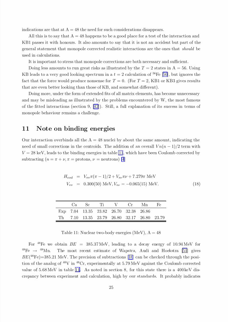
Our interaction overbinds all the A = 48 nuclei by about the same amount, indicating the

need of small corrections in the centroids. The addition of an overall V n(n − 1)/2 term with

V = 28 keV, leads to the binding energies in table 11, which have been Coulomb corrected by

subtracting (n = π + ν, π = protons, ν = neutrons) [4]

H coul = V πππ(π − 1)/2 + V πν πν + 7.279π MeV

V ππ = 0.300(50) MeV, V πν = −0.065(15) MeV. (18)

Ca Sc Ti V Cr Mn Fe

Exp 7.04 13.35 23.82 26.70 32.38 26.86

Th 7.10 13.35 23.79 26.80 32.17 26.80 23.79

Table 11: Nuclear two-body energies (MeV), A = 48

For 48Fe we obtain BE = 385.37 MeV, leading to a decay energy of 10.94 MeV for48Fe → 48Mn. The most recent estimate of Wapstra, Audi and Hoekstra [51] gives

BE (48Fe)=385.21 MeV. The precision of subtractions [16] can be checked through the posi-

tion of the analog of 48V in 48Cr, experimentally at 5.79 MeV against the Coulomb corrected

value of 5.68 MeV in table 11. As noted in section 8, for this state there is a 400 keV dis-

crepancy between experiment and calculation, high by our standards. It probably indicates

25

7/25/2019 FIRAS (463)


the need of some more sophistication in the readjustment of monopole terms than the 28 keV

we have suggested. Note that the theory-experiment differences in table 11 are typical of the

results throughout the paper.

12 Conclusions

Since much of the sections 9 and 10 was devoted to drawing conclusions about the two main

problems addressed, we shall only sum them up:

i) The detailed agreement with the data lends strong support to the claim that minimally

monopole modified realistic forces are the natural and correct choice in structure calcu-

lations.

ii) The description of Gamow-Teller strength is quite consistent with the data, to within

the standard quenching factor. The calculations strongly suggest that dilution due to

fragmentation makes much of the strength unobservable.

Two by-products emerge from the calculations. The first is mainly technical:

iii) Truncations at the t = 3 level are reasonable in the lower part of the pf shell. In general,

however, truncations are a dangerous tool and it would be preferable to replace them by

some other approximation method.

The second by-product is more interesting:

iv) The calculations provide a very clean microscopic view of the notion of intrinsic states

and of the conditions under which rotational motion sets in.

Acknowledgements

This work has been supported in part by the DGICYT (Spain) grant PB89-164 and by the

IN2P3 (France)-CICYT (Spain) agreements.

References

[1] J.N. Ginocchio and J.B. French, Phys. Lett. 7 (1963) 137.

J.N. Ginocchio, Phys. Rev. 144 (1966) 952.

[2] J.D. Mc Cullen, B.F. Bayman and L.Zamick, Phys. Rev. B4 (1964) 515.

[3] H. Horie and K. Ogawa, Nucl. Phys. A216 (1973) 407.

[4] E. Pasquini, Ph. D. Thesis CRN/PT 76-14, Strasburg 1976.

26

7/25/2019 FIRAS (463)


[5] E. Pasquini and A.P. Zuker, “Physics of Medium Light Nuclei”, Florence 1977, P. Blasi

and R. Ricci eds. (Editrice compositrice, Bologna 1978).

[6] A.G.M. van Hess and P.W.M. Glaudemans, Z. Phys. A303 (1981) 267.

[7] R.B.M. Mooy and P.W.M. Glaudemans, Z. Phys. A312 (1983) 59.

[8] R.B.M. Mooy and P.W.M. Glaudemans, Nucl. Phys. A438 (1985) 461.

[9] K. Muto and H. Horie, Phys. Lett. B138 (1984) 9.

[10] A. Yokohama and H. Horie, Phys. Rev. C31 (1985) 1012.

[11] K. Muto, Nucl. Phys. A451 (1986) 481.

[12] J.B. Mc Grory, B.H. Wildenthal and E.C. Halbert, Phys. Rev. C2 (1970) 186.

[13] J.B. Mc Grory and B.H. Wildenthal, Phys. Lett. B103 (1981) 173.

[14] J.B. Mc Grory, Phys. Rev. C8 (1973) 693.

[15] B.J. Cole, J. Phys. G11 (1985) 481.

[16] W.A. Richter, M.G. Van der Merwe, R.E. Julies and B.A. Brown, Nucl. Phys. A523 (1991)

325.

[17] E. Caurier, A. Poves and A.P. Zuker, Phys. Lett. B256 (1991) 301.

[18] K. Ogawa and H. Horie, “Nuclear weak processes an nuclear structure”, M. Morita et al.

eds. (World Scientific, Singapore 1990).


[20] J. Engel, W.C. Haxton and P. Vogel, Phys. Rev. C46 (1992) 2153.

[21] W. Kutschera, B.A. Brown and K. Ogawa, Riv. Nuovo Cimento Vol. 1 no 12 (1978).

[22] A. Poves, E. Pasquini and A.P. Zuker, Phys. Lett. B82 (1979) 319.

[23] A. Poves and A.P. Zuker, Phys. Rep. 70 (1981) 235.

[24] T.W. Burrows, Nuclear Data Sheets 68 (1993) 1.

[25] E. Caurier, Code ANTOINE (Strasburg, 1989).

[26] E. Caurier, A. Poves and A.P. Zuker, Proc. of the Workshop “Nuclear Structure of Light

Nuclei far from Stability. Experiment and Theory.” Obernai. G. Klotz ed. (CRN, Strasburg,

1989).

27

7/25/2019 FIRAS (463)


[27] R.R. Whitehead in “Moment methods in many fermion systems” B.J. Dalton et al. eds.

(Plenum, New York, 1980).

[28] T.T.S. Kuo and G.E. Brown, Nucl. Phys. A114 (1968) 241.

[29] A.R. Edmonds, “Angular Momentum in Quantum Mechanics” (Princeton, N.J. 1960).

[30] D.H. Wilkinson and B.E.F. Macefield, Nucl. Phys. A232 (1974) 58.

[31] W. Bambynek, H. Behrens, M.H. Chen, B. Graseman, M.L. Fitzpatrick, K.W.D. Leding-

ham, H. Genz, M. Mutterer and R.L. Intemann Rev. Mod. Phys. 49 (1977) 77.

[32] D.G. Fleming, O. Nathan, H.B. Jensen and O. Hansen, Phys. Rev. C5 (1972) 1365.

[33] P. Raghavan, Atomic Data and Nuclear Data Tables 42 (1989) 189.

[34] S. Kahana, H.C. Lee and C.K. Scott, Phys. Rev. 180 (1969) 956.

[35] A. Abzouzi, E. Caurier and A.P. Zuker, Phys. Rev. Lett. 66 (1991) 1134.

[36] M. Dufour and A.P. Zuker, preprint CRN 93-29, proposed to Physics Reports, (1993).

[37] H.C. Lee. private communication , (1969).

[38] T. Sekine, J. Cerny, R. Kirchner, O. Klepper, V.T. Koslowsky, A. Plochocki, E. Roeckl,

D. Schardt, B. Shenill and B.A. Brown, Nucl. Phys. A467 (1987) 93.

[39] J. Szerypo, D. Bazin, B.A. Brown, D. Guillemaud-Muller, H. Keller, R. Kirchner, O. Klep-per, D. Morrissey, E. Roeckl, D. Schardt, B. Sherrill, Nucl. Phys. A528 (1991) 203.

[40] E.G. Adelberger, A. Garcia, P.V. Magnus and D.P. Wells, Phys. Rev. Lett. 67 (1991) 3658.

[41] M.B. Aufderheide, S.D. Bloom, D.A. Resler and D.C. Goodman, Phys. Rev. C46 (1992)

2251.

[42] B.A. Brown, Phys. Rev. Lett. 69 (1992) 1034.

[43] A. Cortes and A.P. Zuker, Phys. Lett. B84 (1979) 25.

[44] A. Bohr and B. Mottelson, “Nuclear Structure” (Benjamin, NY 1969).

[45] A.P. Zuker, preprint CRN 92-16, to be published in Nucl. Phys.

[46] A. Abzouzi, J.M. Gomez, C. Prieto and A.P. Zuker, CRN Strasbourg Annual Report

(1990) p.15.

[47] B.H. Wildenthal, Prog. Part. Nucl. Phys. 11 (1984) 5.

[48] B.A. Brown and B.H. Wildenthal, Annual Rev. Nucl. and Part. Sci. 38 (1988) 292.

28

7/25/2019 FIRAS (463)



[50] H. Nakada, T. Otsuka and T. Sebe, Phys. Rev. Lett. 67 (1991) 1086.

[51] A.H. Wapstra, G. Audi and R. Hoekstra, Atomic Data and Nuclear Data Tables 39 (1988)

281.

FIRAS (463)

Documents

Transcript of FIRAS (463)