Finite Word Length Effects and Quantisation Noise

Professors A G Constantinides & L R Arnaut

Finite Word Length Effects Finite Word Length Effects and Quantisation Noiseand Quantisation Noise

1


Finite Word Length EffectsFinite Word Length Effects• Finite register lengths and A/D converters cause errors at different

levels:(i) input:

Input quantisation

(ii) system: Coefficient (= multiplier) quantisation

(iii) output: Operation (products) truncated or rounded due to finite machine word length

2


Input QuantisationInput Quantisation• Discretisation of time (sampling) vs. signal values

– For each sample: search nearest level & round off actual value to this level (S&H) ⇒ finite precision digitized value

– Most values cannot be represented exactly⇒ quantisation error e(k)

– Rounded value can be above or below actual value: random bounded fluctuation of quantisation error:⇒ conceived as quantisation noise

t

ei(t),

Q

eo(t)

3)(tnq

)()()( tntete qio +=

sampling

quan

tisat

ion


• Quantisation error e for quantisation step Q:

• Nearest-level rounding ⇒• Q = least significant bit (determines precision, resolution)• Quantisation is irreversible process (⇒ loss of information)

↔ sampling above Nyquist rate4

QuantisationQuantisation Error (Linear)Error (Linear)

Q

Output

Input

2)(

2QkeQ

≤≤−

)(kei

)(keo Linear mid-treadquantiser

ei(k) to stay within dynamic range R to avoid clipping ofeo(k) (overflow error)

R


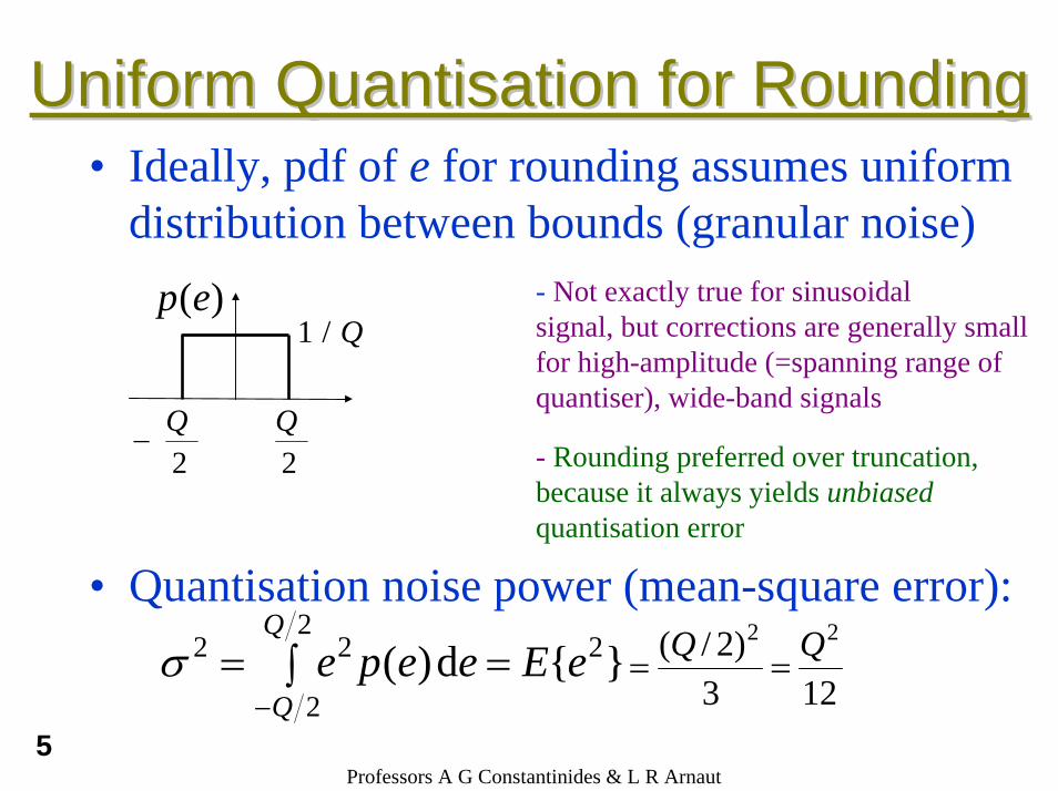
UniformUniform QuantisationQuantisation for Roundingfor Rounding• Ideally, pdf of e for rounding assumes uniform

distribution between bounds (granular noise)- Not exactly true for sinusoidal signal, but corrections are generally small for high-amplitude (=spanning range ofquantiser), wide-band signals

- Rounding preferred over truncation, because it always yields unbiasedquantisation error

• Quantisation noise power (mean-square error):

5

2Q−

2Q

Q/1

∫ ==−

2

2

222 }{d)(Q

QeEeepeσ

123)2/( 22 QQ==

)(ep


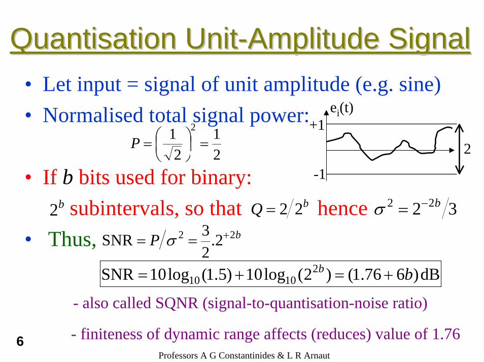
QuantisationQuantisation UnitUnit--Amplitude SignalAmplitude Signal• Let input = signal of unit amplitude (e.g. sine) • Normalised total signal power:

• If b bits used for binary: subintervals, so that hence

• Thus,

- also called SQNR (signal-to-quantisation-noise ratio)

- finiteness of dynamic range affects (reduces) value of 1.766

bQ 22= 32 22 b−=σbP 22 2.

23SNR +== σ

+1

-1

ei(t)

2

b2

21

21 2

=⎟⎠⎞

⎜⎝⎛=P

dB)676.1()2(log10)5.1(log10SNR 21010 bb +=+=


ApplicationsApplications

7

• DECT (speech)• One requires: SNR > 25 dB, i.e., 4 bits• In practice:

– extra 30 dB of dynamic range required – largest signal for nonsinusoidal signal corresponds to 0 dB, not -3 dB

• Thus, -30-25=-55 dB below maximum; requires minimum 9 bit-encoding

• HiFi (e.g., CD/DVD, in-flight data streaming): • Min. 12 bit-encoding (SNR = 78.3 dB); typ. 16-bit (96 dB) because of

imperfect A/D devices

• In practice: using companders (compressor+expander):• Pre-emphasis of input signal before quantisation• Takes advantage of nonuniform probability of analogue values• Result: nonuniformly quantised output signal (use small Q when signal is

small) ⇒ S-shaped (nonlinear) I/O characteristic• Noise reduction in audio: Dolby, dbx


CompandersCompanders• Comparison:

– Uniform quantization, 7 bits + 1 sign bit: SNR=44 dB– Nonuniform quantisation (nonlinear transformation):

• µ-255 characteristic (US, Japan) (UNIX sound, JAVA, etc.):– Exploits logarithmic characteristic of loudness (human sound perception)– Allows for digitization of speech using only 8 bits for SNR=77dB

• A-87.6 characteristic (Europe): international convention

11,)1ln(|)|1ln()sgn()( +<<−

++

= xxxxfµ

µ

⎪⎪⎩

⎪⎪⎨

⎧

≤≤++

≤≤+=

1||/1,)ln(1

||ln1)sgn(

/1||0,)ln(1

||)sgn()(

xAAAxx

AxA

xAxxf

8


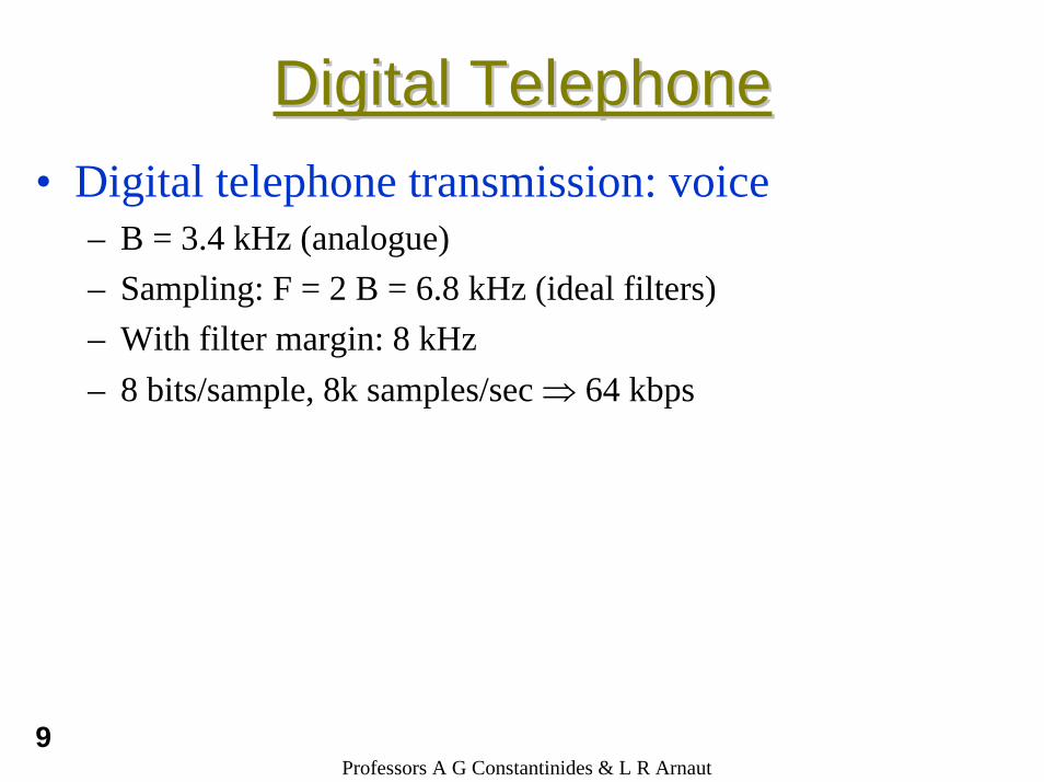
Digital TelephoneDigital Telephone• Digital telephone transmission: voice

– B = 3.4 kHz (analogue)– Sampling: F = 2 B = 6.8 kHz (ideal filters)– With filter margin: 8 kHz– 8 bits/sample, 8k samples/sec ⇒ 64 kbps

9


Multilevel CodingMultilevel Coding• Data transmission: Multilevel coding

– Instead of transmission of single bits: grouping bits, e.g., in pairs:

• lower symbol rate (i.e., smaller channel bandwidth) or higher bit rate, but decoding more difficult (larger quantisation error, or larger power needed)

• Illustrates the dilemma “noise vs. bandwidth (speed) vs. accuracy vs. power”

– Symbol rate (modulation rate) = 1 / duration of 1 pulse• Expressed in baud

– Bit rate = symbol rate × number of bits per symbol• Expressed in bps

– In multilevel coding: symbol rate ≠ bit rate

00

01

10

11

10

Professors A G Constantinides & L R Arnaut11

Coefficient Quantisation: Coefficient Quantisation: SecondSecond--Order SystemsOrder Systems

• Consider a simple example of finite precision of the coefficients a,b of a second order system with two complex conjugate poles :

where

• Quantisation error of coefficients affects location of poles andzeroes ⇒ imperfect frequency response

• Sensitivity of frequency response of filter to quantisation error is minimised if filter is implemented as cascade of 2nd-order filters (can be shown)

2111)( −− ++

=bzaz

zH

θρ je±

221cos211

−− +−=

zz ρθρ

2ρ=b,cos2 θρ−=a


Coefficient QuantisationCoefficient Quantisation

• For

instability (oscillation) can occur fori.e., when poles of H(z) are either

• (i) both on unit circle when complex, or• (ii) one real pole outside unit circle

• Instability under the "effective pole" model is considered as follows

)1(1)( 2

21

1−− ++

=zbzb

zH

12 ⎯→⎯<b

12


Effective Pole ModelEffective Pole Model• In the time domain, from :

• With , instability issue meansis indistinguishable from ,

where represents quantisation operation

)()()( zX

zYzH =

)2()1()()( 21 −−−−= nybnybnxny

12 →b[ ])2(2 −nybQ )2( −ny

[ ]⋅Q

13


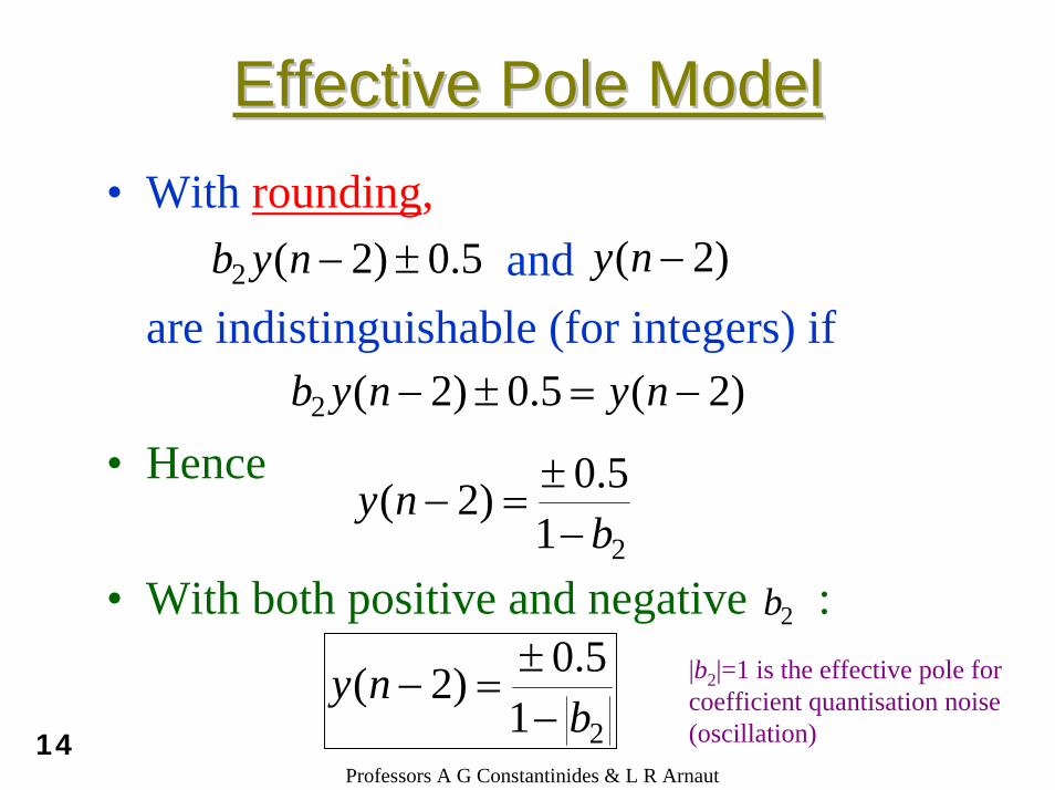
Effective Pole ModelEffective Pole Model• With rounding,

and are indistinguishable (for integers) if

• Hence

• With both positive and negative :

5.0)2(2 ±−nyb )2( −ny

)2(5.0)2(2 −=±− nynyb

215.0)2(

bny

−±=−

215.0)2(

bny

−±=−

2b

|b2|=1 is the effective pole for coefficient quantisation noise (oscillation)14


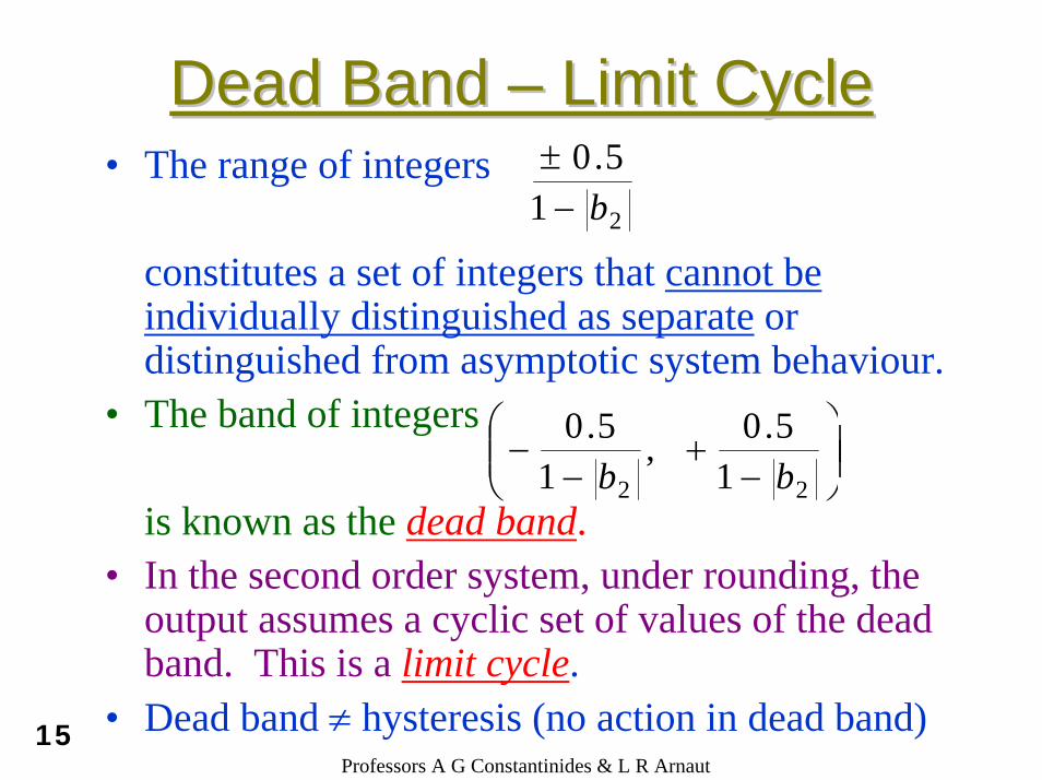
Dead Band Dead Band –– Limit CycleLimit Cycle• The range of integers

constitutes a set of integers that cannot be individually distinguished as separate or distinguished from asymptotic system behaviour.

• The band of integers

is known as the dead band.• In the second order system, under rounding, the

output assumes a cyclic set of values of the dead band. This is a limit cycle.

• Dead band ≠ hysteresis (no action in dead band)

215.0

b−±

⎟⎟⎠

⎞⎜⎜⎝

⎛−

+−

−22 1

5.0 ,1

5.0bb


Effective Pole: OscillationsEffective Pole: Oscillations• Consider the transfer function

• If poles are complex then discrete impulse (unit sample) response sequence is

with

)1(1)( 2

21

1−− ++

=zbzb

zG

2211 −− −−= kkkk ybybxy

kh

[ ]θθ

ρ )1(sin.sin

+= khk

k

,2b=ρ ⎟⎠⎞

⎜⎝⎛−= −

2

112cos b

bθ

16


Effective Pole: OscillationsEffective Pole: Oscillations

• If then the response is sinusoidal (oscillatory) with angular frequency

• Thus, product quantisation causes instability implying an “effective pole“ at .

12 =b

⎟⎠⎞⎜

⎝⎛−= −

2cos1 11 bT

ω

12 =b

17


• Consider infinite precision computations for

Limit Cycle of 2Limit Cycle of 2ndnd Order System: Order System: ExampleExample

21 9.0 −− −+= kkkk yyxy

0 ;00 ; 0

100

<=≠=

=

kykx

x

k

k

-10 -5 0 5 10-10

-8

-6

-4

-2

0

2

4

6

8

10

y k-1

yk

(k=1)(k=2)

(k=3)response converges to the origin without limit

18


Limit Cycle of 2Limit Cycle of 2ndnd Order System: Order System: ExampleExample

• Now the same operation with integer precision

-10 -5 0 5 10-10

-8

-6

-4

-2

0

2

4

6

8

10 -Reponse does not converge to the origin, but assumes cyclically a set of values with nondecreasing quantisation error: the Limit Cycle

-System can only be driven out of its limit cycle only if new & sufficiently large input is applied

-Truncation (as opposed to rounding) can eliminate most limit cycles. However, trun-cation can cause biased quantisation error


Output QuantisationOutput Quantisation• Linear modelling of product quantisation

modelled as

Now interested in output of multiplier

x(n) )(~ nx[ ]⋅Q

x(n)

q(n)

+ )()()(~ nqnxnx +=

20


Output QuantisationOutput Quantisation• Recall: for rounding operations, q(n) is

uniformly distributed between and , where Q is the quantisation step (i.e. in a word length of b bits with sign+magnitude representation mod 2, )

• A discrete-time system with quantisation at the output of each multiplier may be considered as a multi-input linear system

2Q

−2

Q

bQ −= 2

21


Output QuantisationOutput Quantisation

• Each qλ(n) contributes to output accuracy• Then

where is the impulse response of the system from th output of the multiplier to y(n).

h(n)

)()...()...( 21 nqnqnq p

{ })(nx { })(ny

∑ ⎥⎦⎤

⎢⎣⎡ ∑ −+∑ −=

=

∞

=

∞

=

p

rrrnhrqrnhrxny

1 00)().()().()(

λλλ

)(nhλλ

22


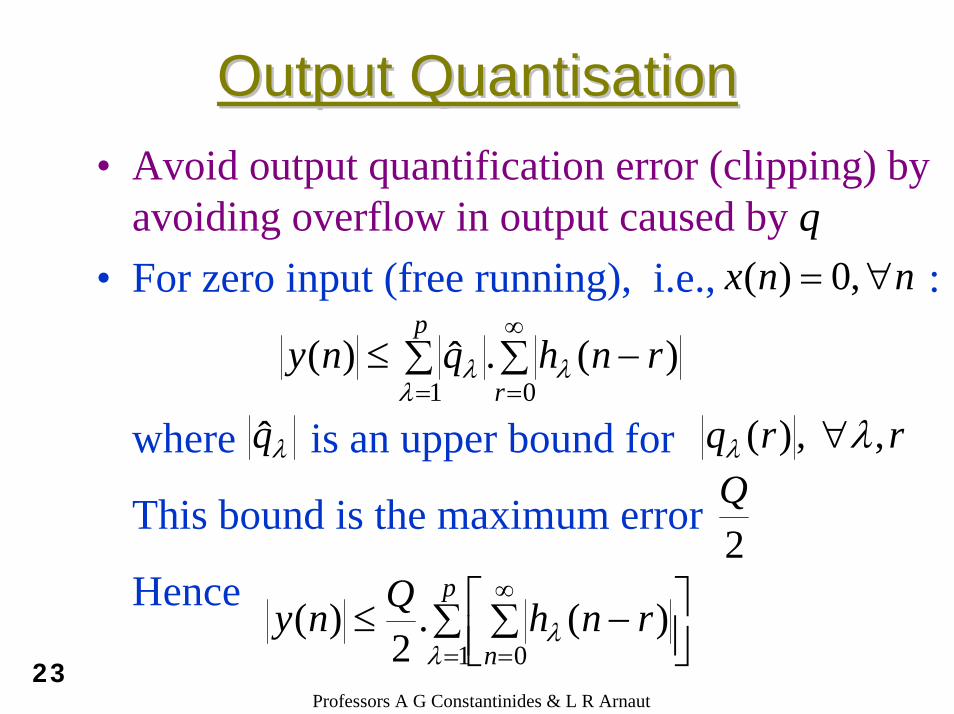
Output QuantisationOutput Quantisation• Avoid output quantification error (clipping) by

avoiding overflow in output caused by q• For zero input (free running), i.e., :

where is an upper bound for

This bound is the maximum error

Hence

nnx ∀= ,0)(

∑ ∑ −≤=

∞

=

p

rrnhqny

1 0)(.ˆ)(

λλλ

λq̂ rrq , ,)( λλ ∀

2Q

∑ ⎥⎦⎤

⎢⎣⎡ ∑ −≤

=

∞

=

p

nrnhQny

1 0)(.

2)(

λλ

23


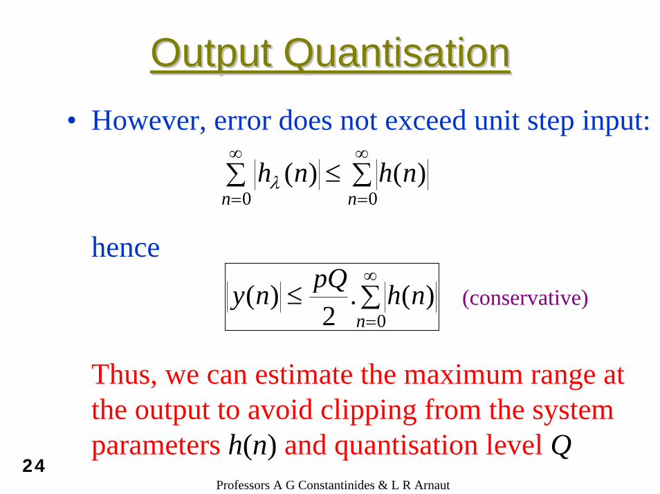
Output QuantisationOutput Quantisation• However, error does not exceed unit step input:

hence

Thus, we can estimate the maximum range at the output to avoid clipping from the system parameters h(n) and quantisation level Q

∑ ∑≤∞

=

∞

=0 0)()(

n nnhnhλ

∑≤∞

=0)(.

2)(

nnhpQny (conservative)

24

Finite Word Length Effects and Quantisation Noise

Documents

Transcript of Finite Word Length Effects and Quantisation Noise