Finite-Time Lyapunov Analysisand Optimal Control

Erkut Aykutlug∗, Kenneth D. Mease∗∗University of California, Mechanical and Aerospace Engineering, Irvine, CA, USA

Abstract— Hyper-sensitive optimal control problemspresent difficulty for general purpose solvers. A numericalimplementation of an approach analogous to the method ofmatched asymptotic expansions requires determining initialand final conditions on appropriate invariant manifolds tosufficient accuracy. Finite-time Lyapunov exponents andvectors are employed for this purpose. The approach is ex-plained and illustrated in the context of a simple transparentexample.

I. INTRODUCTION

Numerical methods for solving optimal control prob-lems (OCPs) can be divided into two main categories,direct and indirect. Indirect methods involve solving theassociated Hamiltonian boundary value problem (HBVP)for an extremal solution that satisfies the first-order neces-sary conditions. A survey of direct and indirect methods,noting their advantages and disadvantages, is given in [5].

An OCP is called hyper-sensitive if the final timeis large relative to some of the contraction and expan-sion rates of the associated Hamiltonian system [13],[14]. The solution to a hyper-sensitive problem can bequalitatively described in three segment as “take-off”,“cruise” and “landing” analogous to optimal flight of anaircraft between distant locations. The “cruise” segmentis primarily determined by the cost function and the statedynamics, whereas the “take-off” and “landing” segmentsare determined by the boundary conditions and the goal ofconnecting these to the “cruise” segment. As the final timeincreases so does the duration of the cruise segment whichshadows a slow reduced-order manifold. When the finaltime is large, the sensitivity of the final state to the un-known initial conditions makes the HBVP ill-conditioned.The ill-conditioning can be removed by approximatingthe solution with a composite one: a concatenation ofboundary-layer solutions (take-off/landing segments) witha solution segment on the slow manifold (cruise segment).The completely hyper-sensitive case is a degenerate casefor which the ’cruise segment’ is near-equilibrium motion,and rather than a slow manifold, there is an equilibriumpoint. The more general case in which the cruise segmentshadows a trajectory on the slow manifold is calledpartially hyper-sensitive.

Solution approximation for completely hyper-sensitiveoptimal control problems, based on the geometric struc-ture of the associated Hamiltonian dynamics, has beenaddressed in [2], [13]. The solution to the HBVP issuch that the solution in the initial boundary layer isapproximated by a trajectory on the stable manifold of

the equilibrium point, the solution in the final boundarylayer is approximated by a trajectory on the unstablemanifold of the equilibrium, and the boundary layersolutions are approximately matched at the equilibriumpoint. The focus of the present paper is on determiningthe unknown boundary conditions such that the solutionend points lie on the appropriate invariant manifolds tosufficient accuracy.

Rather than use information related to the equilibriumpoint which would not be available in the partially hyper-sensitive case, our approach uses a dichotomic basisfor the phase space tangent bundle to define conditionssatisfied by points on the stable and unstable manifoldsof an equilibrium point. Dichotomy transformations havebeen used to solve boundary-value problems for ordinarydifferential equations [3], and to solve fixed end-pointoptimal control problems [2], [17]. Chow used dichotomytransformations to solve nonlinear HBVPs with linearboundary-layer dynamics [7]. For nonlinear HBVPs, adichotomic basis has been approximated using eigen-values and eigenvectors [13] and finite-time Lyapunovexponents and vectors [16]. The latter information canprovide greater accuracy and is more generally applicable[11], [12]. Finite-time Lyapunov exponents, and in somecases vectors, have also been used to analyze fluids [8],[9], [15] and atmospheric circulation [6].

II. FINITE-TIME LYAPUNOV ANALYSIS

In previous work [11] and [12] finite-time Lyapunovanalysis (FTLA) was applied to autononmous nonlineardynamical systems to define and diagnose two-timescalebehavior and compute points on a slow manifold, ifone exists. The approach is to decompose the tangentbundle into subbundles on the basis of the characteristicexponential rates for the associated linear flow, and thento translate the tangent bundle structure into manifoldstructure in the base space. In FTLA, the characteristicexponential rates and associated directions are given,respectively, by finite-time Lyapunov exponents (FTLEs)and finite-time Lyapunov vectors (FTLVs). This approachhas been guided by the asymptotic theory of partiallyhyperbolic invariant sets [4]. The finite-time tangent bun-dle decomposition can be viewed as an approximationof the asymptotic Oseledec’s decomposition [4]. It hasbeen established in [12] that under certain conditionsthe finite-time decomposition approaches the (suitablydefined) asymptotic decomposition exponentially fast, the

0 5 10 15 201 17−1.5

−1

−0.5

0

0.5

1

Time

x(t)

Initial BoundaryLayer Solutions

Final BoundaryLayer Solutions

EquilibriumSolution

Wu

Ws

(0,0)

!1 !0.5 0 0.5 1!0.5

0

0.5

1

1.5

2

2.5

3

x

!

tf = 1

tf = 3

tf = 5

tf = 10

tf = 15

Student Version of MATLAB

1

Fig. 1. Optimal solutions from GESOP c© for different final times,tf = 1, 5, 10, 15 and 17, where x(0) = 1 and x(tf ) = −1 in thetime domain (left) and in the phase space (right).

rate being given by the size of the gaps in the spectrumof the FTLEs.

III. SOLUTION APPROXIMATION STRATEGY FOR ACOMPLETELY HYPER-SENSITIVE PROBLEM

We use a simple transparent example to present theapproximate solution strategy, and later to address someimplementation issues, for a completely hyper-sensitiveoptimal control problem. Consider Lam’s optimal controlproblem [10]: determine the control u∗ and correspondingstate trajectory x∗ that minimize the cost

J =12

∫ tf

0

u2dt (1)

subject to the dynamic constraint

x = sinx+ u (2)

for a given final time tf and boundary conditions x(0) =1 and x(tf ) = −1. The first-order necessary conditionslead to the following Hamiltonian boundary value prob-lem (HBVP)

x = sinx− λλ = −λ cosx

x(0) = 1, x(tf ) = −1(3)

for extremal solutions. Defining the Hamiltonian H =(1/2)u2 + λ(sinx + u) and the phase p = (x, λ)T , wecan write the state/costate dynamics in (3) in the formp = h(p), where h = (∂H/∂λ,−∂H/∂x)T , to show thatwe are dealing with a Hamiltonian system.

We have solved the OCP using the optimization pro-gram GESOP c© [1] for different final times; see Fig. 1.GESOP has several options, of these we used the directmultiple shooting method. The optimal trajectory andcontrol are determined. Using the necessary condition,u∗ = −λ, the solutions can be plotted in the (x, λ) phaseplane. We see that as the final time gets larger the solutiontrajectories shadow more and more closely branches ofthe stable, Ws, and unstable, Wu, invariant manifoldsof the equilibrium point, peq , at (0, 0), and the solutionspends more and more time near the equilibrium point.As tf gets beyond 17, obtaining a numerical solution withGESOP c© gets more and more difficult. In contrast, astf increases, the following approximate solution becomesmore and more accurate and no harder to obtain.

For sufficiently large final times, the optimal strategycan be viewed in phase space as getting on Ws(peq)

where x(0) = 1 and steering along it to the equilibriumpoint and then steering along Wu(peq) to reach the pointon it where x(tf ) = −1. Consistent with this viewpoint,the solution to a completely hyper-sensitive OCP, p∗(t),can be approximated by the composite function

p(t) =

ps(t) 0 ≤ t ≤ tibl

peq tibl < t ≤ tfbl

pu(t) tfbl ≤ t ≤ tf(4)

where ps(t) is the approximate initial boundary-layersolution for t ∈ [0, tibl] with the initial condition onthe stable manifold, i.e., ps(0) = (x0, λ0) ∈ Ws(peq);peq is the equilibrium solution which approximates theslow “cruise” segment; and pu(t) is the approximatefinal boundary-layer solution for t ∈ [tfbl, tf ] with thefinal condition on the unstable manifold, i.e., pu(tf ) =(xtf

, λtf) ∈ Wu(peq). The solutions in the boundary-

layers can be constructed by integrating, in forward andbackward time respectively, the Hamiltonian dynamicsfrom initial and final phase points on the correspondinginvariant manifolds that satisfy the boundary conditions.The composite approximate solution is obtained by con-catenating the boundary-layer solutions with the equilib-rium solution. The times, tibl and tfbl, defining the initialand final boundary-layer durations are selected such thatps and pu reach the equilibrium point up to a specifiedaccuracy in forward and backward time respectively.

The primary challenge in developing this approach isto determine the unknown boundary conditions such thatthe initial and final phase points are sufficiently closeto Ws(peq) and Wu(peq) respectively. The choice tobase our approach on finite-time Lyapunov exponentsand vectors (FTLE/Vs), rather than use other methodsparticularly suited to the structure near the equilibriumpoint, is driven by the goal of extending the approach tothe partially hyper-sensitive case.

IV. DIAGNOSING HYPER-SENSITIVITY

If numerical solution of an OCP using a softwarepackage such as GESOP c© proves difficult and reducingthe final time alleviates the difficulty, hyper-sensitivityshould be investigated. By observing how the solutionevolves as tf is varied, the relevant phase space region canbe identified. Computing the FTLE spectrum at selectedphase points in this region can quantify the exponentialrates. If the spectrum uniformly separates into fast stable,slow, and fast unstable subsets, and the ‘fast’ rates areindeed fast relative to the time interval of interest, thenhyper-sensitivity is confirmed. To describe the generalcase, let n be the dimension of the state dynamics; thenit follows that 2n is the dimension of the associatedHamiltonian system. The spectrum also reveals the equaldimensions, nfs and nfu, of the fast stable and fastunstable behavior, respectively. If nfs + nfu = 2n, thenthe OCP is completely hyper-sensitive for sufficientlylarge tf . If nfs + nfu < 2n, then the OCP is partiallyhyper-sensitive for sufficiently large tf .

An important issue is how to select T , the averagingtime. Lyapunov exponents are averages of the pointwiseexponential rates, i.e., the averages of the appropriatekinematic eigenvalues (KEs) [3], over a segment of atrajectory of the Hamiltonian system. Points of the tra-jectory segment can be indexed by elapsed time. As longas the trajectory evolves in a phase space region wherethe KEs are uniform, larger averaging time T allowsfurther progress in convergence of both the FTLEs andthe FTLVs and better information. However once thetrajectory enters a region of different KEs this ceases to betrue. In Lam’s problem, there is a qualitative differencebetween the local FTLEs and the asymptotic Lyapunovexponents. The two asymptotic Lyapunov exponents arezero at all points except points on the heteroclinic orbitsconnecting the equilibria. On the other hand, the FTLEscan indicate the hyperbolic nature of the dynamics in aneighborhood of a stable or unstable manifold associatedwith an equilibrium point. This is also the observation thatled to the maximum FTLE method that has been used toidentifying Lagrangian coherent structures in fluids [8],[9], [15].

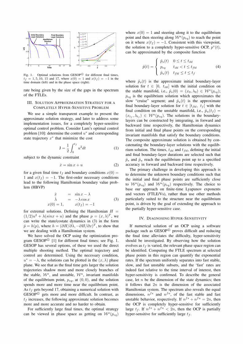
A systematic approach to selecting the averaging timeT such that the FTLEs indicate the local nature ofthe flow to sufficient accuracy, for a flow with non-uniform kinematic eigenvalues is as follows. Fig. 2 showstrajectories that shadow the invariant manifolds of theequilibria. The KE for the vector field h(p), given by

ρh(t) =12hT (p)((Dh(p))T +Dh(p))h(p) (5)

was computed along these trajectories. The red circlesmark points where the ρh is zero; it is positive on oneside of such a point and negative on the other. The positivesign indicates that neighboring points on the trajectory areseparating with time, and negative sign indicates that theyare getting closer to each other. Thus the red circles markthe boundaries separating regions of uniform (in sign)ρh. The time T should be selected to average as longas possible over a uniform region. Fig. 3 shows for a gridof λ(0) values, the trajectories that evolve in forward timefrom the corresponding initial phase points. The zero-crossing for ρh are indicated, as are the times T overwhich the FTLE/Vs can be computed to determine thestable subspace. Although some of the trajectories beginin a different uniform region, most of the time stated isspent in the uniform region where the attraction to theequilibrium point is sensed. Fig. 4 shows that with properselection of T , the maximum FTLE contours identify thestable and unstable manifolds of (0, 0).

V. APPROXIMATE SOLUTION CONSTRUCTION

To implement the solution approximation strategy, weneed to compute λ(0) such that the point p(0) =(x(0), λ(0))T is on the stable manifold Ws. The FTLAapproach is to determine the point p(0) such thath(p(0)) ∈ Es(p(0)), where Es(p(0)) is the stable sub-space approximation by the span of appropriate Lyapunov

−2 −1 0 1 20

0.5

1

1.5

2

2.5

3

x

λ

costate value Time spent in uniform region

λ = 3.0 T = 0.99λ = 2.9 T = 1.04λ = 2.8 T = 1.12λ = 2.7 T = 1.01λ = 2.6 T = 0.98λ = 2.5 T = 0.99λ = 2.4 T = 1.00λ = 2.3 T = 1.05λ = 2.2 T = 1.11λ = 2.1 T = 1.20λ = 2.0 T = 1.34λ = 1.9 T = 1.52λ = 1.8 T = 1.83λ = 1.7 T = 2.84λ = 1.6 T = 2.13λ = 1.5 T = 1.80λ = 1.4 T = 1.59λ = 1.3 T = 1.40λ = 1.2 T = 1.21λ = 1.1 T = 1.03λ = 1.0 T = 0.83

Student Version of MATLAB

Fig. 3. Trajectories starting at p(0) = (1, λ(0)) for a grid of λ(0)values. On each trajectory the zero ρh points are noted. The maximumaveraging time is noted for each value of λ(0).

!

!

"#$#%&

#

#

!% !'() ' '() %!%

!'()

'

'()

%

'(&

'(*

'(+

'(,

%

Fig. 4. Level contours of the FTLE field for the Hamiltonian systemin (3) on a grid of points M = {(x, λ) ∈ R2| x ∈ [−1, 1], λ ∈[−1, 1]}.

vectors. To accomplish this, we determine λ(0) such that〈h(p(0)), w〉 = 0 for all w ∈ Es(p(0))⊥.

Fig. 2 shows the ‘lines of ambiguity’ at x = −π/2 andx = π/2. At these values of x, the orthogonality conditionis satisfied for all values of λ and cannot be used toidentify the particular value of λ that would place p on theappropriate invariant manifold. For all other values of x inthis range, there are isolated solutions to the orthogonalitycondition corresponding to the desired manifolds.

An analogous procedure is followed to place the finalphase point on the unstable manifold.

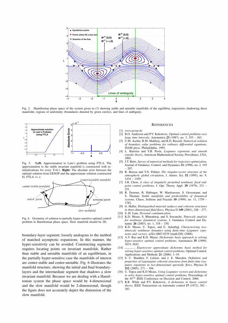
Applying this approach, the solution approximation toLam’s optimal control shown in Fig. 5 was obtained.

VI. PARTIALLY HYPER-SENSITIVE OPTIMALCONTROL PROBLEMS

The consideration of completely hyper-sensitive OCPsin this paper is just a stepping stone to the considerationof partially hyper-sensitive OCPs. Partially hypersensitiveoptimal control problems are associated with HBVPsthat have fast and slow behavior. Ill-conditioning is onlyassociated with certain directions. An accurate approx-imation to the solution of a partially hyper-sensitiveproblem can be constructed from three components: ashort duration initial boundary-layer segment, a longduration slow segment, and a short duration terminal

−4 −3 −2 −1 0 1 2 3 4−4

−3

−2

−1

0

1

2

3

4

5

x

!

Lines of ambiguity

W u (0,0)W s (−",0)

W s (0,0)W u (",0)

Equilibrium points

Points where KE cross zero

Direction of the flow

Fig. 2. Hamiltonian phase space of the system given in (3) showing stable and unstable manifolds of the equilibria, trajectories shadowing thesemanifolds, regions of uniformity (boundaries denoted by green circles), and lines of ambiguity.

−1 −0.5 0 0.5 10

0.2

0.4

0.6

0.8

1

1.2

1.4

1.6

1.8

x

λ

Approximate solutionto Lam’s Problem

using FTLA

−1 −0.5 0 0.5 10

1

2

3

4

5 x 10−3

x

Abso

lute

Err

or

Fig. 5. Left: Approximation to Lam’s problem using FTLA. Theapproximation to the stable invariant manifold is constructed with re-initializations for every T=0.1. Right: The absolute error between theoptimal solution from GESOP and the approximate solution constructedby FTLA vs x.

Fig. 6. Geometry of solution to partially hyper-sensitive optimal controlproblem in Hamiltonian phase space. Slow manifold should be 2D.

boundary-layer segment; loosely analogous to the methodof matched asymptotic expansions. In this manner, thehyper-sensitivity can be avoided. Constructing segmentsrequires locating points on invariant manifolds. Ratherthan stable and unstable manifolds of an equilibrium, inthe partially hyper-sensitive case the manifolds of interestare center-stable and center-unstable. Fig. 6 illustrates themanifold structure, showing the initial and final boundary-layers and the intermediate segment that shadows a slowinvariant manifold. Because we are dealing with a Hamil-tonian system the phase space would be 4-dimensionaland the slow manifold would be 2-dimensional, thoughthe figure does not accurately depict the dimension of theslow manifold.

REFERENCES

[1] www.gesop.de.[2] B.O. Anderson and P.V. Kokotovic, Optimal control problems over

large time intervals, Automatica 23 (1987), no. 3, 355 – 363.[3] U.M. Ascher, R.M. Mattheij, and R.D. Russell, Numerical solution

of boundary value problems for ordinary differential eqautions,SIAM press, Philadelphia, 1995.

[4] L. Barreira and Y.B. Pesin, Lyapunov exponents and smoothergodic theory, American Mathematical Society, Providence, USA,2002.

[5] J.T. Betts, Survey of numerical methods for trajectory optimization,Journal of Guidance, Control, and Dynamics 21 (1998), no. 2, 193– 207.

[6] R. Buizza and T.N. Palmer, The singular-vector structure of theatmospheric global circulation, J. Atmos. Sci. 52 (1995), no. 9,1434 – 1459.

[7] J.H. Chow, A class of singularly perturbed nonlinear, fixed end-point control problems, J. Opt. Theory Appl. 29 (1979), 231 –251.

[8] R. Doerner, B. Hubinger, W. Martienssen, S. Grossmann, andS. Thomae, Stable manifolds and predictability of dynamicalsystems, Chaos, Solitons and Fractals 10 (1999), no. 11, 1759 –1782.

[9] G. Haller, Distinguished material surfaces and coherent structuresin three-dimensional fluid flows, Physica D 149 (2001), 248 – 277.

[10] S.-H. Lam, Personal communication.[11] K.D. Mease, S. Bharadwaj, and S. Iravanchy, Timescale analysis

for nonlinear dynamical systems, J. Guidance Control and Dy-namic 26 (2003), no. 1, 318 – 330.

[12] K.D. Mease, U. Topcu, and E. Aykutlug, Characterizing two-timescale nonlinear dynamics using finite-time Lyapunov expo-nents and vectors, arXiv:0807.0239 [math.DS] (2008).

[13] A.V. Rao and K.D. Mease, Dichotomic basis approach to solvinghyper-sensitive optimal control problems, Automatica 35 (1999),3633–3642.

[14] , Eigenvector approximate dichotomy basis method forsolving hyper-sensitive optimal control problems, Optimal Control:Applications and Methods 21 (2000), 1–19.

[15] S. C. Shadden, F. Lekien, and J. E. Marsden, Definition andproperties of Lagrangian coherent structures from finite-time Lya-punov exponents in two-dimensional aperiodic flows, Physica D212 (2005), 271 – 304.

[16] U. Topcu and K.D Mease, Using Lyapunov vectors and dichotomyto solve hyper-sensitive optimal control problems, Proceedings ofthe 45th IEEE Conference on Decision and Control, 2006.

[17] R.R. Wilde and P.V. Kokotovic, A dichotomy in linear controltheory, IEEE Transactions on Automatic control 17 (1972), 382 –383.