Finite Sample Properties of Semiparametric Estimators of ...jmccrary/BDM2008_v11.pdf · assignment...
61
Finite Sample Properties of Semiparametric Estimators of Average Treatment Effects * Matias Busso University of Michigan John DiNardo University of Michigan and NBER Justin McCrary University of Californa, Berkeley and NBER October 8, 2008 Abstract We explore the finite sample properties of several semiparametric estimators of average treat- ment effects, including propensity score reweighting, matching, double robust, and control function estimators. When there is good overlap in the distribution of propensity scores for treatment and control units, reweighting estimators are preferred on bias grounds and attain the semiparametric efficiency bound even for samples of size 100. Pair matching exhibits sim- ilarly good performance in terms of bias, but has notably higher variance. Local linear and ridge matching are competitive with reweighting in terms of bias and variance, but only once n = 500. Nearest-neighbor, kernel, and blocking matching are not competitive. When overlap is close to failing, none of the estimators examined perform well and √ n -asymptotics may be a poor guide to finite sample performance. Trimming rules, commonly used in the face of problems with overlap, are effective only in settings with homogeneous treatment effects. JEL Classification: C14, C21, C52. Keywords: Treatment effects, propensity score, overlap, irregular identification, semipara- metric efficiency. Preliminary draft. Please do not distribute or cite without permission. Comments welcome. * For comments that improved the paper, we thank Alberto Abadie, Matias Cattaneo, Marie Davidian, Keisuke Hirano, Jack Porter and Guido Imbens. We would also like to thank Markus Fr¨ olich for providing us copies of the code used to generate the results in his paper.
Transcript of Finite Sample Properties of Semiparametric Estimators of ...jmccrary/BDM2008_v11.pdf · assignment...
Finite Sample Properties of Semiparametric
Estimators of Average Treatment Effects∗
Matias BussoUniversity of Michigan
John DiNardoUniversity of Michigan
and NBER
Justin McCraryUniversity of Californa, Berkeley
and NBER
October 8, 2008
Abstract
We explore the finite sample properties of several semiparametric estimators of average treat-ment effects, including propensity score reweighting, matching, double robust, and controlfunction estimators. When there is good overlap in the distribution of propensity scores fortreatment and control units, reweighting estimators are preferred on bias grounds and attainthe semiparametric efficiency bound even for samples of size 100. Pair matching exhibits sim-ilarly good performance in terms of bias, but has notably higher variance. Local linear andridge matching are competitive with reweighting in terms of bias and variance, but only oncen = 500. Nearest-neighbor, kernel, and blocking matching are not competitive. When overlapis close to failing, none of the estimators examined perform well and
√n -asymptotics may
be a poor guide to finite sample performance. Trimming rules, commonly used in the face ofproblems with overlap, are effective only in settings with homogeneous treatment effects.
JEL Classification: C14, C21, C52.
Keywords: Treatment effects, propensity score, overlap, irregular identification, semipara-metric efficiency.
Preliminary draft.Please do not distribute or cite without permission.
Comments welcome.
∗For comments that improved the paper, we thank Alberto Abadie, Matias Cattaneo, Marie Davidian, KeisukeHirano, Jack Porter and Guido Imbens. We would also like to thank Markus Frolich for providing us copies of thecode used to generate the results in his paper.

Contents
I Introduction 1
II Notation and Background 4A Estimands and Estimators . . . . . . . . . . . . . . . . . . . . . . . . . . . . . . . . 5B Weighted Least Squares as a Unifying Framework . . . . . . . . . . . . . . . . . . . 6C Mixed Methods . . . . . . . . . . . . . . . . . . . . . . . . . . . . . . . . . . . . . . 10D Tuning Parameter Selection . . . . . . . . . . . . . . . . . . . . . . . . . . . . . . . 12E Efficiency Bounds . . . . . . . . . . . . . . . . . . . . . . . . . . . . . . . . . . . . . 12
IIIData Generating Process 14
IV Results: Benchmark Case 16A Correct Parametric Specification of Treatment Assignment . . . . . . . . . . . . . . 17B Incorrect Specification of Treatment Assignment . . . . . . . . . . . . . . . . . . . . 19
V Problems with Propensity Scores Near Boundaries 20
VI Results: Boundary Problems 24A Simulation Results with Boundary Problems . . . . . . . . . . . . . . . . . . . . . . 25B Trimming . . . . . . . . . . . . . . . . . . . . . . . . . . . . . . . . . . . . . . . . . 26
VIIReconciliation with Previous Literature 27
VIIIConclusion 31
Appendix I: Derivation of IPW3 for TOT 33
Appendix II: Derivation of SEB for proposed DGPs 36
Bibliography 44

I Introduction
This paper explores the finite sample properties of semiparametric estimators of average treatment
effects. Such estimators are standard in the program evaluation literature and have become increas-
ingly popular in the applied microeconometric literature. These estimators rely on two assumptions.
The first assumption is that assignment to treatment is randomized conditional on a set of observed
covariates. The second assumption is more technical and asserts that no value of the observed co-
variates assures treatment assignment.1 Intuitively, these assumptions allow for treatment to covary
with observed characteristics, but require that there be some unexplained variation in treatment
assignment left over after conditioning and that the unexplained aspect of treatment resembles an
experiment.2
Estimation of program impacts under these assumptions could proceed using traditional para-
metric estimation methods such as maximum likelihood. However, an early result of Rosenbaum
and Rubin (1983) is that if treatment is randomized conditionally on the observed covariates, then it
is randomized conditional on the (scalar) propensity score, the conditional probability of treatment
given the observed covariates. Influenced by this result, the subsequent econometric and statistical
literatures have focused on semiparametric estimators that eschew parametric assumptions on the
relationship between the outcome and observed covariates. Empirical literatures, particularly in
economics, but also in medicine, sociology and other disciplines, feature an extraordinary number
of program impact estimates based on such semiparametric estimators.
Perhaps surprisingly in light of their ubiquity in empirical work, formal large sample results
for these estimators have only recently been derived in the literature. Heckman, Ichimura and
Todd (1997) report large sample properties of estimators based on kernel and local linear matching
on the true and an estimated propensity score. Hirano, Imbens and Ridder (2003) report large
sample properties of a reweighting estimator that uses a nonparametric estimate of the propensity
score. This is essentially the same reweighting estimator that was introduced to the economics
literature by DiNardo, Fortin and Lemieux (1996) and Dehejia and Wahba (1997), and it is related
to an estimator due to Horvitz and Thompson (1952). Importantly, Hirano et al. (2003) establish
that their version of a reweighting estimator achieves the semiparametric efficiency bound (SEB)
established by Hahn (1998) for this problem. Robins, Rotnitzky and Zhao (1994) and Robins
and Rotnitzky (1995) establish large sample properties and the efficiency of a regression-adjusted
reweighting estimator that uses the estimated propensity score. Finally, Abadie and Imbens (2006)
establish the large sample properties and near-efficiency of kth nearest-neighbor matching using the
1Selection on observed variables is defined in Section II, as is the second assumption, which is typically referred toas an overlap assumption. In Section III, we emphasize the correct interpretation of selection on observed variablesusing a specific parametric model.
2In other words, there exists an instrument which is unobserved by the researcher.
1

true propensity score.3
To date, no formal finite sample properties have been established for any of the estimators
discussed, and there is limited simulation evidence on their performance. It is generally desirable
to learn about the finite sample properties of estimators used in empirical research, since not all
data sets are big enough for asymptotic theory to be a useful guide to estimator properties. It is
particularly desirable to learn about the finite sample properties of semiparametric estimators of
average treatment effects, given the literature’s substantive focus on treatment effect heterogeneity.4
In the face of heterogeneity, treatment effects must effectively be estimated for various subsamples.5
For many economic data sets, these subsamples are modest in size, perhaps numbering in the
hundreds or even dozens, where asymptotic theory may be a particularly poor guide to finite sample
performance.
In this paper, we examine the relative performance of several leading semiparametric estimators
of average treatment effects in samples of size 100 and 500.6 We focus on the performance of propen-
sity score reweighting and matching estimators for estimating the average treatment effect (ATE)
and the average effect of treatment on the treated (TOT). We consider a range of matching strate-
gies, including nearest neighbor, kernel, local linear, and ridge matching, and blocking. We also
consider several varieties of reweighting estimators, the so-called double robust estimator (Robins
et al. 1994), and a specific version of Hahn’s (1998) general estimator, which we term a control
function estimator. We consider settings with good overlap in the distribution of propensity scores
for treatment and control units, as well as settings of poor overlap. In settings of poor overlap,
we investigate the performance of various trimming methods proposed and used in the literature.
Finally, we consider the implications for performance of misspecification of the propensity score,
both in terms of an incorrect parametric model for treatment as well as conditioning on the wrong
set of covariates.
A summary of our findings is as follows. First, reweighting is approximately unbiased and
3It deserves mention that Chen, Hong and Tarozzi (2008) study the large sample properties and efficiency of sieveestimators in this setting. We do not study the finite sample properties of these estimators due to space constraints.
4Understanding the sources of treatment effect heterogeneity is critical if the analyst hopes to extrapolate fromthe findings of a given study to broader forecasts of the likely impacts of policies not yet implemented. These issuesare a key focus of the program evaluation literature (see, for example, Heckman and Vytlacil 2005 and Heckman,Urzua and Vytlacil 2006).
5Importantly, the intrinsic dimensionality of treatment effect heterogeneity cannot be massaged by appealingto the dimension reduction of the propensity score. The Rosenbaum and Rubin (1983) result that a conditionallyrandomized treatment is randomized conditional on the scalar propensity score has been interpreted as justification formatching on the propensity score rather than on the full set of covariates. However, the Rosenbaum and Rubin resultdoes not imply that units with the same value of the propensity score have the same treatment effect. Examplesof empirical investigation of treatment effect heterogeneity along dimensions different from the propensity scoreinclude Card (1996), Katz, Kling and Liebman (2001), Haviland and Nagin (2005) and Kent and Hayward (2008),for example.
6This issue has been previously taken up by Lunceford and Davidian (2004), Frolich (2004), Zhao (2004), Zhao(2008), and Freedman and Berk (n.d.).
2

semiparametrically efficient, even for sample sizes of 100. Our assessment is that reweighting exhibits
the best overall finite sample performance of any of the estimators we consider. Second, pair
matching shares the good bias performance of reweighting, but has a variance that is roughly 30
percent greater than that of reweighting. Third, kth nearest-neighbor matching, with k chosen by
leave-one-out cross-validation, does reduce the excessive variance of pair matching, but at the cost
of substantially greater bias. Fourth, kernel, local linear, and ridge matching perform similarly to
k-th nearest neighbor matching in exhibiting little variance but much bias when n = 100. Once
n = 500, ridge and local linear matching are both competitive with reweighting on bias and variance
grounds.7 Fifth, both in terms of bias and variance, the popular blocking matching estimator
performs neither as badly as kth nearest-neighbor and kernel matching, nor as well as local linear
and ridge matching, and is generally dominated by reweighting. Sixth, the double robust estimator
is competitive with reweighting, but appears to be slightly more variable and slightly more biased.
Seventh, the control function estimator is approximately unbiased, even for samples of size 100, and
is approximately semiparametrically efficient once n = 500. Eighth, when there is misspecification
of the propensity score either due to parametric assumptions or the lack of availability of important
covariates, the relative performance of the estimators is approximately as described above. However,
in that context, if problems with bias are suspected and variance is less important, pair matching
is the preferred estimator.
The above conclusions hold when the propensity score model is correctly specified and when
there is good overlap in the distribution of propensity scores for treatment and control units. Our
investigations highlight the problems with semiparametric estimators of average treatment effects
when overlap is poor. Khan and Tamer (2007) emphasize this point from a theoretical perspective,
noting that when overlap is poor the semiparametric efficient bound derived by Hahn (1998) for
this problem can be infinite, leading to a failure of√n-consistency. Consistent with this conclusion,
our results indicate that when overlap is poor, none of the estimators studied work well. In cases
where overlap is poor, although technically sufficient to guarantee√n-consistency, we document
poor performance for n = 100, but adequate performance for n = 500. This suggests that larger
sample sizes may be needed for threshold cases.
A standard empirical approach to problems with overlap is to trim observations with extreme
values of the propensity score. We investigate four of the trimming strategies used in the literature.
Our simulations suggest that some of these procedures can be effective but only in situations in
which the treatment effect is similar for all the observations in the sample. Finally, we provide
evidence that as problems with overlap arise, the limiting distribution of semiparametric estimators
becomes nonstandard.
Our conclusions run contrary to those of the existing literature on the finite sample performance
7All three of these kernel-based estimators use leave-one-out cross-validation to select a bandwidth, and this modelselection issue may be an important aspect of performance for smaller sample sizes.
3
of reweighting and matching. Our simulations indicate that reweighting is a generally robust es-
timator whose performance in small samples is as effective as in large samples, where it has been
shown to be optimal in a certain sense. The matching methods we consider work poorly for samples
of size 100, although some of the methods become effective for samples of size 500. In contrast
to these findings, the existing finite sample literature is generally negative regarding reweighting
and tends to conclude that matching estimators are best. We review this literature. We show
that nearly all of the results from the existing finite sample literature are based on data generating
processes (DGPs) for which√n-consistent semiparametric estimators do not exist, or DGPs where
√n-consistency is close to failing. Our own investigations are unusual, in that we focus on DGPs
where semiparametric estimators are expected to perform well. We show that this difference in
DGPs accounts for our different conclusions.8
The remainder of the paper is organized as follows. Section II sets notation, defines estimators,
discusses estimands and efficiency bounds, and emphasizes the connections among the many esti-
mators we consider by casting them in the common framework of weighted regression. In particular,
this section provides a 3-step interpretation of matching that clarifies the conceptual similarities
and differences between the two approaches. In Section III, we describe our benchmark DGP. This
DGP is chosen so that semiparametric estimates of average treatment effects are√n-consistent.
Results for the benchmark DGP are presented in Section IV. In Section V, we take up the issue
of DGPs for which√n-consistency may be compromised. Results for such DGPs are presented in
V. Section VII compares our results to those of the existing finite sample literature. Section VIII
concludes.
II Notation and Background
Let Yi(1) denote the outcome for unit i that would obtain under treatment and Yi(0) the outcome
that would obtain under control. Treatment is denoted by the binary variable Ti. We observe
Yi = TiYi(1)+(1−Ti)Yi(0), but never the pair (Yi(0), Yi(1)). The data (Xi, Yi, Ti)ni=1 are taken to be
independent across i, but are potentially heteroscedastic. Let the propensity score, the conditional
probability of treatment, be denoted p(x) ≡ P (Ti = 1|Xi = x). Let the covariate-specific average
treatment effect by denoted τ(x) = E[Yi(1)− Yi(0)|Xi = x].
We focus on the relative performance of semiparametric estimators of population averages of
τ(x). Here, semiparametric means an estimator that models the relationship between the proba-
bility of receiving treatment and the covariates Xi, but remains agnostic regarding the relationship
between the counterfactual outcomes (Yi(0), Yi(1)) and the covariates.
8To be clear, we do not advocate the use of reweighting estimators—or any of the estimators studied here—insettings of failure and near failure of
√n-consistency of semiparametric estimators of average treatment effects. At
present, relatively little is known about appropriate estimation and testing procedures in these settings.
4

Semiparametric estimators of treatment effects are typically justified by an appeal to (1) selec-
tion on observed variables and (2) sufficient overlap. Selection on observed variables means that
treatment is randomized given Xi, or that (Yi(0), Yi(1), Zi)⊥⊥Ti|Xi, where Zi is any characteristic
of the individual that is not affected by treatment assignment (e.g. pre-program earnings).9This
assumption has traditionally been referred to as selection on observed variables in the economics
literature (e.g., Heckman and Robb 1985). In the statistics and more recent econometrics literature
this assumption is instead referred to as ignorability or unconfoundedness (e.g., Rosenbaum and
Rubin 1983, Imbens 2004).10
Selection on observed variables is not by itself sufficient to semiparametrically identify average
treatment effects. The DGPs we focus on in Section IV are consistent with both selection on
observed variables and a strict overlap assumption: ξ < p(x) < 1 − ξ for almost every x in the
support of Xi, for some ξ > 0. This assumption is stronger than the standard overlap assumption
that 0 < p(x) < 1 for almost every x in the support of Xi (e.g., Rosenbaum and Rubin 1983,
Heckman et al. 1997, Hahn 1998, Wooldridge 2002, Imbens 2004, Todd 2007), but is also common
in the literature (e.g., Robins et al. 1994, Abadie and Imbens 2006, 2008, Crump, Hotz, Imbens
and Mitnik 2007a,b). Both the standard overlap and the strict overlap assumptions are strong.
Khan and Tamer (2007) emphasize that something akin to the strict overlap assumption is needed
to deliver√n-consistency of semiparametric estimators in this context. We take up the issue of
DGPs that violate strict overlap, but satisfy standard overlap, in Sections V and VI, below.
A Estimands and Estimators
As noted, we focus on the performance of estimators for target parameters that are averages of
τ(x). The specific averages we consider are the average treatment effect α = E[τ(Xi)] and the
average treatment effect on the treated θ = E[τ(Xi)|T = 1]. We refer to these estimands as ATE
and TOT, respectively. Although we focus on the performance of estimators for these estimands,
we emphasize that ATE and TOT are not the only estimands of interest. However, the performance
of these estimators for ATE and TOT is likely to be similar to the performance of these estimators
when adapted to estimation of other averages of τ(x).
We consider fourteen estimators: nine matching estimators, three reweighting estimators (some-
times termed inverse propensity score weighting estimators, or IPW), one control function estimator,
and the so-called double robust estimator.11 Each of these estimators are two-step estimators re-
9Notice that some pre-program covariates may be affected by anticipation of treatment.10Lechner (2005) shows that some control variables may be influenced by the treatment. However, this endogeneity
does not matter for consistency of the treatment effect estimator, as long as the usual formulation of the conditionalindependence assumption holds.
11The breadth of coverage arises from an attempt to encompass many of the estimators used in the literature aswell as to be consistent with previous finite sample evidence on the topic. Nonetheless, there are of course otherpotentially effective estimators whose performance is not covered by the analysis here.
5

lying on a first-step estimate of the propensity score. The nine matching estimators include pair
matching, kth nearest neighbor matching, kernel matching, local linear matching, ridge regression
matching, and blocking. Aside from pair matching, each of these matching strategies employs a
cross-validation method for choosing a tuning parameter. Kernel, local linear, and ridge matching all
further require the choice of a kernel. Following Frolich (2004), we consider both the Epanechnikov
kernel and the Gaussian kernel.
The three reweighting estimators include a reweighting estimator in which the sum of the weights
is allowed to be stochastic (IPW1), a reweighting estimator in which the sum of the weights is forced
to be 1 (IPW2), and an asymptotically optimal combination of the former two estimators (IPW3)
that is due to Lunceford and Davidian (2004).
We also consider the so-called double robust estimator due to Robins and Rotnitzky (1995),
which has recently received a good deal of attention in the literature (e.g., Imbens 2004). This
procedure can be thought of as a regression-adjusted version of reweighting. The regression ad-
justments are more similar in spirit to an older approach to the problem of estimating treatment
effects. We complete our analysis by studying the performance of a control function estimator. This
estimator is essentially the same as the double robust estimator, but is unweighted. The version of
the control function estimator we implement models the regression function of the outcome given
the covariates and treatment status as a polynomial in the estimated propensity score, with addi-
tive and possibly interacted terms for treatment status. This procedure is described in Wooldridge
(2002) for the case of ATE, and is in the spirit of Oaxaca (1973) and Blinder (1973) decompositions
and Hahn’s (1998) general estimator.
While it is true that at least some versions of reweighting and matching are believed to be
semiparametrically efficient in large samples, and while both approaches are based on the same first-
step propensity score estimate, it is far from clear that the two approaches would perform similarly
in finite samples. First, most matching estimators rely on tuning parameters. It is possible that use
of tuning parameters could improve finite sample performance relative to reweighting. Second, the
approaches take advantage of very different properties of the propensity score. Matching requires of
the estimated propensity score only that it be a balancing score (Rosenbaum and Rubin 1983). In
contrast, reweighting requires that the propensity score be a conditional probability. For example,
matching on the square root of the propensity score should work just as well as matching on
propensity score; in contrast, reweighting with the square root of the propensity score should do
badly.
B Weighted Least Squares as a Unifying Framework
Both matching and reweighting estimators of average treatment effects can be understood as the
coefficient on the treatment indicator in a weighted regression, with weighting functions that differ
6
by estimator. This common structure clarifies that the essential difference between the estimators
is the weighting function implicitly used.
That reweighting estimators have this form is widely understood. A general notation for
reweighting estimators for the TOT and ATE is
θ =1
n1
n∑i=1
TiYi −1
n0
n∑j=1
(1− Tj)Yjw(j), (1)
α =1
n1
n∑i=1
TiYiw1(i)− 1
n0
n∑j=1
(1− Tj)Yjw0(j). (2)
The weights in equations (1) and (2) only add up to one for some versions of reweighting estimators.
When the TOT weights add up to one in the sense of 1n0
∑nj=1(1− Tj)w(j) = 1, the TOT estimate
can be obtained using standard statistical software from the coefficient on treatment in a regression
of the outcome on a constant and a treatment indicator using weights W = T + (1−T )w(·). When
the weights do not add up to one, the TOT estimate can be calculated directly using equation
(1). When the ATE weights add up to one in the sense that 1n0
∑nj=1(1 − Tj)w0(j) = 1 and
1n1
∑nj=1 Tjw1(j) = 1, the ATE estimate can be obtained from the same regression described, but
with weights W = Tw1(·) + (1−T )w0(·). The reweighting estimators we consider are characterized
below by enumerating the weighting functions used.
Weights Used for Reweighting EstimatorsEffect Treatment, t Estimator Weighting Function wt(j)
TOT 1 IPW1p(Xj)
1−p(Xj)
/p
1−p
TOT 1 IPW2p(Xj)
1−p(Xj)
/1n0
∑nk=1
(1−Tk)p(Xk)1−p(Xk)
TOT 1 IPW3p(Xj)
1−p(Xj)(1− Cj)
/1n0
∑nk=1
(1−Tk)p(Xk)1−p(Xk)
(1− Ck)ATE 0 IPW1 1−p
1−p(Xj)
ATE 1 IPW1 pp(Xj)
ATE 0 IPW2 11−p(Xj)
/1n0
∑nk=1
1−Tk
1−p(Xk)
ATE 1 IPW2 1p(Xj)
/1n1
∑nk=1
Tk
p(Xk)
ATE 0 IPW3 11−p(Xj)
(1− C0j )/
1n0
∑nk=1
1−Tk
1−p(Xk)(1− C0
k)
ATE 1 IPW3 1p(Xj)
(1− C1j )/
1n1
∑nk=1
Tk
p(Xk)(1− C1
k)
Note: p ≡ n1
n, Ai = 1−Ti
1−p(Xi), Bi = Ti
p(Xi), Ci =
“1− p(Xi)
pAi
”1n
Pnj=1
„1−
p(Xj)
pAj
«1n
Pnj=1
„1−
p(Xj)
pAj
«2 ,
C0i =
11−p(Xi)
1n
Pnj=1(Aj p(Xj)−Ti)
1n
Pnj=1(Aj p(Xj)−Ti)
2 and C1i =
1p(Xi)
1n
Pnj=1(Bj(1−p(Xj))−(1−Ti))
1n
Pnj=1(Bj(1−p(Xj))−(1−Ti))
2 , which are
IPW3 correction factors that are small when the propensity score model is well specified.
The functional form given by IPW1 can be found in many treatments in the literature (e.g.,
7
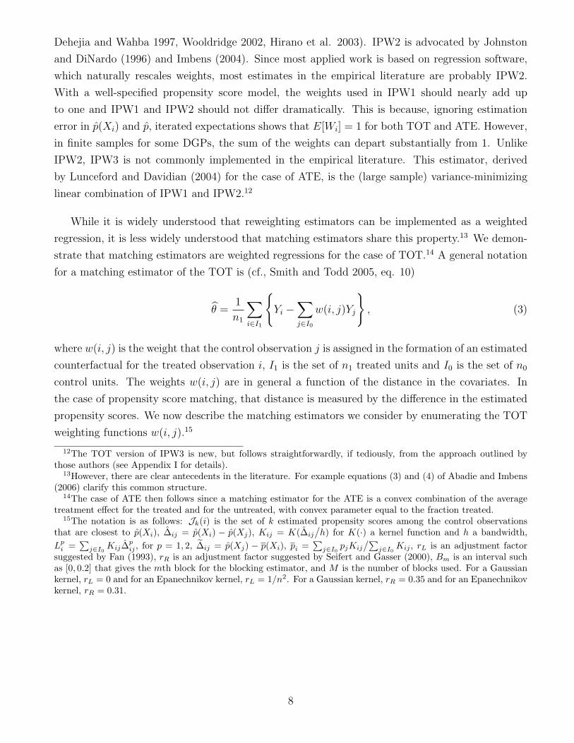
Dehejia and Wahba 1997, Wooldridge 2002, Hirano et al. 2003). IPW2 is advocated by Johnston
and DiNardo (1996) and Imbens (2004). Since most applied work is based on regression software,
which naturally rescales weights, most estimates in the empirical literature are probably IPW2.
With a well-specified propensity score model, the weights used in IPW1 should nearly add up
to one and IPW1 and IPW2 should not differ dramatically. This is because, ignoring estimation
error in p(Xi) and p, iterated expectations shows that E[Wi] = 1 for both TOT and ATE. However,
in finite samples for some DGPs, the sum of the weights can depart substantially from 1. Unlike
IPW2, IPW3 is not commonly implemented in the empirical literature. This estimator, derived
by Lunceford and Davidian (2004) for the case of ATE, is the (large sample) variance-minimizing
linear combination of IPW1 and IPW2.12
While it is widely understood that reweighting estimators can be implemented as a weighted
regression, it is less widely understood that matching estimators share this property.13 We demon-
strate that matching estimators are weighted regressions for the case of TOT.14 A general notation
for a matching estimator of the TOT is (cf., Smith and Todd 2005, eq. 10)
θ =1
n1
∑i∈I1
{Yi −
∑j∈I0
w(i, j)Yj
}, (3)
where w(i, j) is the weight that the control observation j is assigned in the formation of an estimated
counterfactual for the treated observation i, I1 is the set of n1 treated units and I0 is the set of n0
control units. The weights w(i, j) are in general a function of the distance in the covariates. In
the case of propensity score matching, that distance is measured by the difference in the estimated
propensity scores. We now describe the matching estimators we consider by enumerating the TOT
weighting functions w(i, j).15
12The TOT version of IPW3 is new, but follows straightforwardly, if tediously, from the approach outlined bythose authors (see Appendix I for details).
13However, there are clear antecedents in the literature. For example equations (3) and (4) of Abadie and Imbens(2006) clarify this common structure.
14The case of ATE then follows since a matching estimator for the ATE is a convex combination of the averagetreatment effect for the treated and for the untreated, with convex parameter equal to the fraction treated.
15The notation is as follows: Jk(i) is the set of k estimated propensity scores among the control observationsthat are closest to p(Xi), ∆ij = p(Xi) − p(Xj), Kij = K(∆ij
/h) for K(·) a kernel function and h a bandwidth,
Lpi =∑j∈I0 Kij∆
pij , for p = 1, 2, ∆ij = p(Xj) − p(Xi), pi =
∑j∈I0 pjKij
/∑j∈I0 Kij , rL is an adjustment factor
suggested by Fan (1993), rR is an adjustment factor suggested by Seifert and Gasser (2000), Bm is an interval suchas [0, 0.2] that gives the mth block for the blocking estimator, and M is the number of blocks used. For a Gaussiankernel, rL = 0 and for an Epanechnikov kernel, rL = 1/n2. For a Gaussian kernel, rR = 0.35 and for an Epanechnikovkernel, rR = 0.31.
8

Weights Used for Matching Estimators for TOTEstimator Weighting Function w(i, j)kth Nearest Neighbor 1
k1(p(Xj)∈Jk(i))
Kernel Kij
/∑j∈I0 Kij
Local Linear(KijL
2i −Kij∆ijL
1i
)/∑j∈I0
(KijL
2i −Kij∆ijL
1i + rL
)Ridge Kij
/∑j∈I0 Kij + ∆ij
/∑j∈I0
(Kij∆
2ij + rRh|∆ij|
)Blocking
∑Mm=1 1(p(Xi)∈Bm)1(p(Xj)∈Bm)
/∑Mm=1 1(p(Xj)∈Bm)
All of the matching estimators enumerated can be understood as the coefficient on the treatment
indicator in a weighted regression. To see this, rewrite
θ =1
n1
n∑i=1
Ti
{Yi −
n∑j=1
w(i, j)(1− Tj)Yj
}
=1
n1
n∑i=1
TiYi −n∑j=1
(1− Tj)Yj1
n1
n∑i=1
w(i, j)Ti
≡ 1
n1
n∑i=1
TiYi −1
n0
n∑j=1
(1− Tj)Yjw(j), (4)
where w(j) = n0
n1
∑ni=1 w(i, j)Ti is proportional to the average weight that a control observation is
given, on average across all treatment observations.16 Viewing matching estimators as weighted
least squares is useful as a means of understanding the relationships among the various estimators
used in the literature. For example, the weight used by kernel matching can be written as
w(j) =n0
n1
n∑i=1
Tiw(i, j) =
∑ni=1 TiKij
/∑ni=1 Kij∑n
j=1(1− Tj)Kij
/∑ni=1Kij
/p
1− p.
Ignoring estimation error in the propensity score,∑n
i=1 TiKij
/∑ni=1Kij is a kernel regression
estimate of P (Ti = 1|p(Xi) = p(Xj)), which is equivalent to p(Xj).17 If the kernel in ques-
tion is symmetric, then∑n
i=1(1− Ti)Kij
/∑ni=1Kij is similarly a kernel regression estimate of
P (Ti = 0|p(Xi) = p(Xj)), which is equivalent to 1 − p(Xj). Thus, for kernel matching with a
16The matching estimators proposed in the literature require no normalization on the weights involved in the secondsum in equation (4). This follows because the matching estimators that have been proposed define the weightingfunctions w(i, j) in such a way that
∑j∈I0 w(i, j)Yj is a legitimate average of the controls, in that sense that for
every treated unit i,∑j∈I0 w(i, j) =
∑nj=1 w(i, j)(1− Tj) = 1. This has the important implication that the weights
in the second sum of equation (4) automatically add up to one:
1n0
n∑j=1
(1− Tj)w(j) =1n0
n∑j=1
{(1− Tj)
[n0
n1
n∑i=1
w(i, j)Ti
]}=
1n1
n∑i=1
Ti∑j∈I0
w(i, j)
=1n1
n∑i=1
Ti = 1.
17Generally, if X and Y are random variables such that m(X) = E[Y |X] exists, then E[Y |m(X)] = m(X) byiterated expectations.
9

symmetric kernel, we have
w(j) ≈ p(Xj)
1− p(Xj)
/p
1− p,
which is the same as the target parameter of the TOT weight used by reweighting.
This result provides a 3-step interpretation to symmetric kernel matching for the TOT:
1. Estimate the propensity score, p(Xi)
2. For each observation j in the control group, compute p(Xj) =∑n
i=1 TiKij
/∑ni=1Kij. In
words, this is the fraction treated among those with propensity scores near p(Xj). Undersmoothness assumptions on p(Xi), this will be approximately p(Xj).
3. Form the weight w(j) =(p(Xj)
/(1− p(Xj)
)/ (p/
(1− p))
and run a weighted regression of
Yi on a constant and Ti with weight Wi = Ti + (1− Ti)w(i).
Reweighting differs from this procedure in that, in step 2, it directly sets p(Xj) = p(Xj). The
simulation suggests that this shortcut is effective at improving small sample performance.
C Mixed Methods
We also consider the performance of an estimator known as “double robust” that is neither reweight-
ing nor matching but is a hybrid procedure combining reweighting with more traditional regression
techniques. This procedure is discussed by Robins and Rotnitzky (1995) in the related context of
imputation for missing data. Imbens (2004) provides a good introductory treatment.
To describe the intuition behind this estimator, we first return to a characterization of reweight-
ing. The essential idea behind reweighting is that in large samples, reweighting ensures orthogonal-
ity between the treatment indicator and any possible function of the covariates. That is, for any
bounded continuous function g(·),
E [g(Xi)|Ti = 1] = E
[g(Xi)
p(Xi)
1− p(Xi)
/ p
1− p
∣∣∣Ti = 0
],
E
[g(Xi)
p
p(Xi)
∣∣∣Ti = 1
]= E
[g(Xi)
1− p1− p(Xi)
∣∣∣Ti = 0
]= E [g(Xi)] . (5)
This implies that the joint distribution of Xi is equal in weighted subsamples defined by Ti = 1
and Ti = 0, using either TOT or ATE weights.18 This in turn implies that in the reweighted
sample, treatment is unconditionally randomized, and estimation can proceed by computing the
(reweighted) difference in means, as described in subsection B, above. A standard procedure in esti-
mating the effect of an unconditionally randomized treatment is to include covariates in a regression
18Given the standard overlap assumption, this result follows from iterated expectations. A proof for the case ofTOT is given in McCrary (2007, fn. 35).
10

of the outcome on a constant and a treatment indicator. It is often argued that this procedure im-
proves the precision of estimated treatment effects. By analogy with this procedure, a reweighting
estimator may enjoy improved precision if the weighted regression of the outcome on a constant
and a treatment indicator is augmented by covariates.
The estimator just described is the double robust estimator. Reweighting computes average
treatment effects by running a weighted regression of the outcome on a constant and a treatment
indicator. Double robust estimation computes average treatment effects by running a weighted
regression of the outcome on a constant, a treatment indicator, and some function of the covariates
such as the propensity score.
The gain in precision associated with moving from a reweighting estimator to a double robust
estimator is likely modest with economic data.19 However, a potentially important advantage is
that the estimator is more likely to be consistent, in a particular sense. Suppose that the model
for the treatment equation is misspecified, but that the model for the outcome equation is correctly
specified. Then the double robust estimator would retain consistency, despite the misspecification
of the treatment equation model.20 We implement the double robust estimator by including the
estimated propensity score linearly into the regression model, for both ATE and TOT.21
The double robust estimator is related to another popular estimator that we call a control
function estimator. For the case of ATE, the control function estimator is the slope coefficient on
a treatment indicator in a regression of the outcome on a constant, the treatment indicator, and
functions of the covariates Xi. For the case of TOT, we obtain the control function estimator by
running a regression of the outcome on a constant and a cubic in the propensity score, separately by
treatment status.22 For each model, we form predicted values, and compute the average difference
in predictions, among the treated observations. This procedure is in the spirit of the older Oaxaca
(1973) and Blinder (1973) procedure and is related to the general estimator proposed by Hahn
(1998).
19Suppose the goal is to obtain a percent reduction of q in the standard error on the estimated treatment effect.Approximate the standard error of the treatment effect by the spherical variance matrix least squares formula. Thenreducing the standard error of the estimated treatment effect by q percent requires reducing the regression root meansquared error by q percent, since the “matrix part” of the standard error is affected only negligibly by the inclusionof covariates, due to the orthogonality noted in equation (5). This requires reducing the regression mean squarederror (MSE) by roughly 2q percent when q is small. A 2q percent reduction in the regression MSE requires thatthe F -statistic on the exclusion of the added covariates be a very large 2qn/K, where n is the overall sample sizeand K is the number of added covariates. Consider one of the strongest correlations observed in economic data,that between log-earnings and education. In a typical U.S. Census file with 100,000 observations, the t-ratio onthe education coefficient in a log-earnings regression is about 100 (cf., Card 1999). The formula quoted suggeststhat including education as a covariate with an outcome of log earnings would improve the standard error on ahypothetical treatment indicator by only 5 percent.
20In the case described, the double robust estimator would be consistent, but inefficient relative to a regression-based estimator with no weights, by the Gauss-Markov Theorem.
21We include the p(Xi) rather than Xi because the outcome equation in our DGPs is a function of p(Xi).22In simulations not shown, we computed the MSE for the control function estimator in which the propensity score
entered in a polynomial of order 1,...,5. The cubic polynomial had the lowest MSE on average across contexts.
11

D Tuning Parameter Selection
The more complicated matching estimators require choosing tuning parameters. Kernel-based
matching estimators require selection of a bandwidth, nearest-neighbor matching requires choosing
the number of neighbors, and blocking requires choosing the blocks.
In order to select both the bandwidth h to be used in the kernel-based matching estimators
and the number of neighbors to be utilized in nearest neighbor matching, we implement a simple
leave-one-out cross-validation procedure that chooses h as
h∗ = arg minh∈H
∑i∈I0
[Yi − m−i (p (Xi))]2 ,
where m−i (p (Xi)) is the predicted outcome for observation i, computed with observation i removed
from the sample, and m (·) is the non-parametric regression function implied by each matching pro-
cedure. For kernel, local linear and ridge matching the bandwidth search grid H is 0.01× |κ| 1.2g−1
for g = 1, 2, ..., 29,∞. For nearest-neighbor matching the grid H is {1, 2, ..., 20, 21, 25, 29, ..., 53,∞}for a sample size smaller than 500 and {1, 2, 5, 8, .., 23, 28, 33, ..., 48, 60, 80, 100,∞} for 500 or more
observations.23
For the blocking estimator, we first stratify the sample into M blocks defined by intervals of the
estimated propensity score. We continue to refine the blocks until within each block we cannot reject
the null that the expected propensity score among the treated is equal to the expected propensity
score among the controls (Rosenbaum and Rubin 1983, Dehejia and Wahba 1999). In order to
perform this test we used a simple t-test with a 99 percent confidence level. Once the sample is
stratified, we can compute the average difference between the outcome of treated and control units
that belong to each block, τm. Finally, the blocking estimator computes the weighted average of τm
across M blocks, where the weights are the proportion of observations in each block, either overall
(ATE) or among the treated only (TOT).
E Efficiency Bounds
In analyzing the performance of the estimators we study, it useful to have an idea of a lower bound
on the variance of the various estimators for a given model. Estimators which attain a variance
lower bound are best, in a specific sense.
We consider two variants of efficiency bounds. The first of these is the Cramer-Rao lower bound,
which can be calculated given a fully parametric model. The semiparametric models motivating
the estimators under study in this paper do not provide sufficient detail on the putative DGP to
23For more details on this procedure see Stone (1974) and Black and Smith (2004) for an application.
12

allow calculation of the Cramer-Rao bound. Nonetheless, since we assign the DGP in this study,
we can calculate the Cramer-Rao bound using this knowledge. This forms a useful benchmark.
For example, we will see that in some models, the variance of a semiparametric estimator is only
slightly greater than the Cramer-Rao bound. These are then models in which there is little cost to
discarding a fully parametric model in favor of a semiparametric model.
The second efficiency bound we calculate is the semiparametric efficiency bound. These bounds
can be viewed as the smallest variance that can be obtained without imposing parametric assump-
tions on the outcome equation. Alternatively, the SEB can be viewed as the least upper bound
of the Cramer-Rao bounds, among the set of DGPs consistent with the parametric assumptions
placed on the treatment equation. An introductory discussion of the SEB concept is given in Newey
(1990). Hahn (1998, Theorems 1, 2) shows that under selection on observed variables and standard
overlap, the SEB is given by
SEBATEk/u = E
[σ2
1(Xi)
p(Xi)+
σ20(Xi)
1− p(Xi)+ (τ(Xi)− α)2
], (6)
SEBTOTu = E
[σ2
1(Xi)p(Xi)
p2+σ2
0(Xi)p(Xi)2
p2 (1− p(Xi))+p(Xi)
p2(τ(Xi)− θ)2
], (7)
SEBTOTk = E
[σ2
1(Xi)p(Xi)
p2+σ2
0(Xi)p(Xi)2
p2 (1− p(Xi))+p(Xi)
2
p2(τ(Xi)− θ)2
], (8)
where the subindex l = k, u indicates whether the propensity score is known or unknown and σ2t (Xi)
is the conditional variance of Yi(t) given Xi.
Reweighting using a nonparametric estimate of the propensity score achieves the bounds in
equations (6) and (7), as shown by Hirano et al. (2003) for both the ATE and TOT case. Nearest
neighbor matching on covariates using a Euclidean norm also achieves these bounds when the
number of matches is large. Abadie and Imbens (2006, Theorem 5) demonstrate this for the case of
ATE and the case of TOT follows from the machinery they develop.24 However, nearest neighbor
matching is inconsistent when there is more than one continuous covariate to be matched.
Efficiency results for other matching estimators are not yet available in the literature. In Ap-
pendix II we provide a derivation of the SEB for the models used in our simulations. In Appendix
Table A6 we show the SEB and the CRLB for all of the data generating processes used in this
paper. We turn now to a description of these models.
24Using their equation (13) and the results of the unpublished proof of their Theorem 5, it is straightforward toderive the large sample variance of the kth nearest-neighbor matching estimator for the TOT as
SEBTOTu +12kE
[σ2
0(Xi)p
(1
1− p(Xi)− (1− p(Xi))
)]−−−−→k →∞ SEBTOTu (9)
13

III Data Generating Process
The DGPs we consider are all special cases of the latent index model
T ∗i = η + κXi − ui, (10)
Ti = 1 (T ∗i > 0) , (11)
Yi = βTi + γm(p(Xi)) + δTim(p(Xi)) + εi, (12)
where ui and εi are independent of Xi and of each other, m(·) is a curve to be discussed, and
p(Xi) is the propensity score implied by the model, or the probability of treatment given Xi. The
covariate Xi is taken to be distributed standard normal. Our focus is on cross-sectional settings, so
εi is independent across i, but potentially heteroscedastic. This is achieved by generating ei as an
independent and identically distributed standard normal sequence and then generating
εi = ψ (eip(Xi) + eiTi) + (1− ψ)ei. (13)
We consider several different distributional assumptions for the treatment assignment equation
residual, ui. As we discuss in more detail in Sections V and VI below, the choice of distribution
for ui can be relevant to both the finite and large sample performance of average treatment effect
estimators. Let the distribution function for ui be denoted generally by F (·). Then the propensity
score is given by
p(Xi) ≡ P (T ∗i > 0) = F (η + κXi). (14)
The model given in equations (10) through (12) nests a basic latent index regression model, in
which treatment effects vary with Xi but are homogeneous, residuals are homoscedastic, and the
conditional expectation of the outcome under control is white noise. The model is flexible, how-
ever, and can also accommodate heterogeneous treatment effects, heteroscedasticity, and nonlinear
response functions.
Heterogeneity of treatment effects is controlled by the parameter δ in equation (12). When
δ = 0, the covariate-specific treatment effects are constant: τ(x) = β for all x. Thus under this
restriction the average treatment effect (ATE) and the average effect of treatment on the treated
(TOT) both equal β in the population and in the sample.25 When δ 6= 0, the covariate-specific
treatment effect, given by τ(x) = β + δm(p(x)), depends on the covariate and ATE and TOT may
differ.26 Heteroscedasticity is controlled by the parameter ψ in equation (13). When ψ = 0, we
obtain homoscedasticity. When ψ 6= 0, the residual variance depends on treatment as well as on
the propensity score. The function m(·) and the parameter γ manipulate the non-linearity of the
25For a discussion of the distinction between sample and population estimands, see Imbens (2004), for example.26For a discussion of other estimands of interest, see Heckman and Vytlacil (2005), for example.
14

outcome equation that is common to both treated and non-treated observations.27
We assess the relative performance of the estimators described in Section II in a total of twenty-
four different contexts. These different contexts are characterized by four different settings, three
different designs, and two different regression functions. We now describe these contexts in greater
detail.
The four settings we consider correspond to four different combinations of the parameters in
equation (12): β, γ, δ, and ψ. In each of these four settings, we set β = 1 and γ = 1. However,
we vary the values of the parameters δ and ψ, leading to four combinations of homogeneous and
heterogeneous treatment effects and homoscedastic and heteroscedastic error terms. The specific
configurations of parameters used in these four settings are summarized below:
Setting β γ δ ψ Description
I 1 1 0 0 homogeneous treatment, homoscedastic
II 1 1 1 0 heterogeneous treatment, homoscedastic
III 1 1 0 2 homogeneous treatment, heteroscedastic
IV 1 1 1 2 heterogeneous treatment, heteroscedastic
The two regression functions we consider, m(·), correspond to the functional forms used by
Frolich (2004). The first curve considered is a simple linear function. The second curve is non-
linear and rises from around 0.7 at q = 0 to 0.8 near q = 0.4, where the curve attains its peak,
before declining to 0.2 at q = 1. The precise equations used for these two regression functions are
summarized below:
Curve Formula Description
1 m1(q) = 0.15 + 0.7q Linear
2 m2(q) = 0.2 +√
1− q − 0.6(0.9− q)2 Nonlinear
Finally, the three designs we consider correspond to different combinations of the parameters in
equation (10): η and κ. These parameters control degrees of overlap between the densities of the
propensity score of treated and control observations as well as different ratios of control to treated
units. The specific configurations of parameter values for η and κ are different in Sections IV and
VI and are enumerated in those sections.
27Note that we only consider DGPs in which γ 6= 0. When γ = 0, all estimators of the TOT for which the weightingfunction w(j) adds up to 1 can analytically be shown to be finite sample unbiased. When γ 6= 0, no easy analyticalfinite sample results are available, and simulation evidence is much more relevant.
15

IV Results: Benchmark Case
We begin by focusing on the case of Xi distributed standard normal and ui distributed standard
Cauchy.28 As we discuss in more detail below, an initial focus on this DGP allows us to sidestep some
important technical issues that arise with poor overlap in propensity score distributions between
treatment and control units. We defer discussion of these complications until Sections V and VI.
The specific configurations of the parameters η and κ used in these three designs are summarized
below:
Design η κ Treated-to-Control Ratio
A 0 0.8 1:1
B 0.8 1 2:1
C -0.8 1 1:2
An important feature of these DGPs is the behavior of the conditional density functions of the
propensity score, p(Xi), conditional on treatment. Figure 1A displays the conditional density of the
propensity score given treatment status. This figure features prominently in our discussion, and we
henceforth refer to such a figure as an overlap plot.
The figures point to several important features of our benchmark DGPs. First, for all three
designs considered, the strict overlap assumption is satisfied. As noted by Khan and Tamer (2007),
this is a sufficient assumption for√n-consistency of semiparametric treatment effects estimators.
Second, the ratio of the treatment density height to that for control gives the treatment-to-control
sample size ratio. From this we infer that it is more challenging to estimate the TOT in design C
than in designs A or B. Third, design A is symmetric and estimation of the ATE is no more difficult
than estimation of the TOT.
We turn next to an analysis of the results of the simulation. In Section IV.A we assume that the
propensity score model is correctly specified, and estimation proceeds using a maximum likelihood
Cauchy binary choice model that includes Xi as the sole covariate. In Section IV.B we study the
impact of misspecification of the propensity score model on performance.
In both sections IV.A and IV.B, and throughout the paper, we report separate estimates of
the bias and the variance of the estimators. In addition, for each estimator we test the hypothesis
that the bias is equal to zero, and we test the hypothesis that the variance is equal to the SEB.
These choices reflect our view that it is difficult to bound the bias a researcher would face, across
the possible DGPs the researcher might confront, unless the estimator is unbiased or nearly so.
28In principle, we could have let ui follow a normal distribution with parameters selected in a manner that theyallow for good overlap. In such a case, because in the normal case the parameters that manipulate overlap alsochange the ratio of treated to control observations in the designs, we would not be able to explore designs as theones we can study when ui is distributed Cauchy.
16

Bounding the bias is desirable under an objective of minimizing the worst case scenario performance
of the estimator, across possible DGPs.
A Correct Parametric Specification of Treatment Assignment
Table 1 examines the performance of our 14 estimators in the Normal-Cauchy model for n = 100
and n = 500. For ease of exposition, we do not show estimates of the bias and variance for all
twenty-four contexts.29 Instead, we summarize these estimates by presenting the simulated root
mean square bias (RMSB) and average variance, both overall across the twenty-four contexts and
separately for the settings described in Section III.30 There are 14 columns, one for each estimator
under consideration.
Estimates of the RMSB are presented in the first and second panels of Table 1 for n = 100 and
n = 500, respectively. As an aid to summarizing the results, we additionally perform F-tests of
the null hypothesis that the bias is zero jointly across the twenty-four contexts and jointly across
the designs and curves in any given setting.31 The value of the F-statistic for the joint test across
twenty-four contexts is reported below the setting-specific RMSB estimates, and p-values for these
F-tests are reported in brackets.32 The values of the F-statistics for the setting-specific tests are
suppressed in the interest of space. For these tests, we place an asterisk next to the RMSB when
the hypothesis is rejected at the 1% significance level.
Average variances are presented in the third and fourth panels of Table 1 for n = 100 and
n = 500, respectively. We provide a reference point for these variances using the SEB.33 Below the
average variances we report the percentage difference between the estimated variance and the SEB
on average across all twenty-four contexts. We also perform a F-test of the equality of the variance
estimates and the SEB, jointly across all twenty-four contexts and separately for each setting.34 The
29As described above, a context here means a bundle of setting, design, and curve. We consider four settings, threedesigns and two curves.
30In the main text, we focus on TOT and report summary tables. A series of appendix tables present summarytables for ATE. Detailed tables for both TOT and ATE, as well as Stata data sets containing all of the replicationresults, are available at http://www.econ.berkeley.edu/∼jmccrary.
31Practically, these tests are implemented as Wald tests using a feasible generalized least squares model for the240,000 replications less their (context-specific) target parameters. To keep the power of these tests constant acrosssample sizes, we keep nR constant at one million, where R is the number of replications. This implies 10,000replications for n = 100 and 2,000 replications for n = 500. This also spares significant computational expense.
32Logical equivalence of null hypotheses implies that these F-tests can be viewed as (i) testing that all twenty-fourbiases are zero, (ii) testing that all four setting-specific RMSB are zero, or (iii) testing that the overall RMSB is zero.
33Table A6 presents the SEB for each of the twenty-four contexts in question and contrasts this semiparametricbound with the parametric Cramer-Rao bound. Details of these computations are provided in Appendix II. Becausethe overlap is generally good in the Normal-Cauchy model, the SEB is only 8% higher than the Cramer-Rao boundon average across contexts and never more than 28% higher. Note that the variances reported in Table 1 for n = 100are to be compared to 10×SEB (10×SEB = 1000× (SEB/100)) and for n = 500 are to be compared to 2×SEB.
34Practically, these tests are implemented as Wald tests using a generalized least squares model for the twenty-four estimated variances less their (context-specific) SEB. The variance of the variance can be approximated quite
17

F-statistic for the joint test across all twenty-four contexts is presented below the average percent
discrepancy between the variances and the SEBs. For the setting-specific test, we suppress the value
of the statistic in the interest of space. For these tests, we place an asterisk next to the average
variance when the hypothesis is rejected at the 1% significance level.
We turn now to a discussion of the results, beginning with the evidence on bias for n = 100.
The results suggest several important conclusions. First, the pair matching, reweighting, double
robust, and control function estimators are all approximately unbiased. Of these, IPW1 and IPW2
are probably the least biased, performing even better than pair matching. Double robust seems
to acquire slightly greater bias in settings with treatment effect heterogeneity, whereas the other
unbiased estimators acquire slightly less. The F-statistics reject the null of zero bias at the 5% level
of significance for all estimators except IPW1, IPW2, and control function. Second, all matching
estimators that rely upon tuning parameters are noticeably biased. We suspect that this is due to
the difficulty of accurate estimation of nonparametric tuning parameters.35 Of these estimators,
ridge matching performs best, particularly when the Epanechnikov kernel is used.
For n = 500, pair matching, reweighting, double robust and control function remain approxi-
mately unbiased. In terms of bias, these estimators perform remarkably similarly for this sample
size. For the more complicated matching estimators, we see reduced bias in all cases as expected,
and local linear and ridge matching become competitive with reweighting with the larger sample
size. Although we can still reject the null of no bias, blocking becomes much less biased. The bias
of nearest-neighbor and kernel matching remains high in all settings.
When analyzing the performance within settings (see appendix tables) we observe similar pat-
terns of relative performance. First, reweighting, double robust, and control function estimators
are all unbiased regardless of the shape of the overlap plots and regardless of the ratio of treated to
control observations. Second, treatment effect heterogeneity, homoscedasticity, and nonlinearity of
the regression response function all affect relative performance negligibly.
We next discuss the variance results, presented in the bottom half of Table 1. These results reveal
several important findings. First, pair matching presents the largest variance of all the estimators
under consideration in all four settings, for both n = 100 and n = 500. Second, for n = 100, IPW2,
IPW3 and double robust have the lowest variance among unbiased estimators. Once n = 500, the
SEB is essentially attained by all of the unbiased estimators except for pair matching. Compared to
the SEB, IPW3 has on average a variance for n = 100 that is 3.5% in excess, IPW2 a variance that is
accurately under an auxiliary assumption that the estimates of the TOT are distributed normally. In that case, thevariance of the variance is approximately 2V 2/(R− 1), where V is the sample variance itself and R is the number ofreplications. See Wishart (1928) and Muirhead (2005, Chapter 3).
35Loader (1999) reports that the rates of convergence of cross validation is Op(n−1/10) which could explain the badperformance of these estimators in small samples. See also, Galdo, Smith and Black (2007) for further discussion onalternative cross-validation methods.
18

4% in excess, and double robust a variance that is 6.4% in excess. Once n = 500, these percentages
decline to 1%, 1.2%, and 1.4%, respectively.36 Third, among the biased estimators, those with
highest bias (nearest-neighbor and kernel matching) are the ones that present the lowest variance.
On average the variance of these estimators is below the SEB. This suggests that if these estimators
are asymptotically efficient, then they have a variance which approaches the SEB from below. This
conjecture is particularly plausible since local linear and ridge matching, the least biased among
the matching estimators, exhibit variance similar to that of the reweighting estimators.
In sum, our analysis indicates that when good overlap is present and misspecification is not
a concern, there is little reason to use an estimator other than IPW2 or perhaps IPW3. These
estimators are trivial to program, typically requiring 3 lines of computer code, appear to be subject
to minimal bias, and are minimal variance among approximately unbiased estimators.
B Incorrect Specification of Treatment Assignment
We investigate two different types of misspecification of the propensity score. First, we assume that
p (Xi) = F (η + κXi) when in fact the true DGP is p (Xi) = F (η+κX1i+X2i +X3i) whereXji follows
a standard normal distribution and F (·) is a Cauchy distribution. We call this a misspecification
in terms of covariates, Xi. This kind of misspecification occurs when the researcher fails to include
all confounding variables in the propensity score model. Second, we proceed with estimation as if
p (Xi) = F (η + κXi) when in fact the true DGP is p (Xi) = F (η + κXi). In particular, we keep
F (·) as the distribution function for the standard Cauchy, but estimate the propensity score with
a probit—that is, we assume that p(Xi) = Φ(η + κXi). We call this a misspecification in terms of
the treatment equation residual, ui.
Results of these investigations are displayed in Table 2. The structure of this table is similar to
that of Table 1. Table 2 presents the RMSB and average variance for the 14 estimators in a sample
size of 100 under the two types of misspecifications. Covariate misspecification is treated in panels
1 and 3, and distributional misspecification is treated in panels 2 and 4.
The first panel shows that covariate misspecification leads every estimator to become biased in
every setting. This is expected and emphasizes the central role of the assumption of selection on
observed variables. Unless the unexplained variation in treatment status resembles experimental
variation, treatment effects estimators cannot be expected to produce meaningful estimates. These
estimators may continue to play a role as descriptive tools, however. The third panel shows that
36Although IPW1 does notably worse in terms of variance than IPW2, its performance is not as bad as has beenreported in other studies. For instance, Frolich (2004) reports that in a homoscedastic and homogeneous settingIPW1 has an MSE that is between 150% and 1518% higher than that of pair-matching. The good performance ofIPW1 documented in Table 1 is due to the fact that, in the Normal-Cauchy model, there is a vanishingly smallprobability of having an observation with a propensity score close to 1. It is propensity scores near 1 that generateextreme weights, and it is extreme weights that lead to large variance of weighted means.
19
the average variances are always below the SEB, typically by 20% to 30%. Thus, the exclusion
of relevant covariates from the propensity score model may lead to precise estimates of the wrong
parameter.
We turn next to the results on distributional misspecification, where the DGP continues to have
a Cauchy residual on the treatment assignment equation, but the researcher uses a probit model
for treatment. The second panel presents results for the bias in this case. In this situation, only
pair matching and control function remain unbiased. Double robust is approximately unbiased
only in settings of homogeneous treatment effects. The reweighting estimators become biased but
are always less biased than the matching estimators. The fourth panel shows that none of the
estimators achieve the SEB. Unfortunately, the most robust estimators to misspecification of the
propensity score, that is pair matching and control function, are the ones with the largest variance.
Ridge matching and IPW3 are closest to the SEB, differing only by 4% to 6%.
V Problems with Propensity Scores Near Boundaries
The model given in equations (10) to (12) assumes selection on observed variables. As has been
noted by many authors, selection on observed variables is a strong assumption. It is plausible in
settings where treatment is randomized conditional on the function of the Xi given in (12). However,
it may not be plausible otherwise.37 We feel that practitioners appreciate the importance of this
assumption.
However, perhaps less widely appreciated than the importance of the selection on observed vari-
ables assumption is the importance of overlap assumptions. As emphasized by Khan and Tamer
(2007), the model outlined in equations (10) to (12)—while quite general and encompassing all
of the existing simulation evidence on performance of estimators for ATE and TOT under uncon-
foundedness of treatment—does not necessarily admit a√n-consistent semiparametric estimator
for ATE or TOT. In particular, the standard overlap assumption that 0 < p(Xi) < 1 is not sufficient
to guarantee√n-consistency, whereas the strict overlap assumption that ξ < p(Xi) < 1−ξ for some
ξ > 0 is. However, the strict overlap assumption can be violated by the model in equations (10) to
(12). For example, Khan and Tamer (2007) note that√n-consistency is violated in the special case
of Xi and ui both distributed standard normal, with η = 0 and κ = 1. The following proposition
sharpens this important result.
Proposition. Under the model specified in equations (10) to (12), with Xi and ui distributed stan-
dard normal, boundedness of the conditional variance of ei given Xi, and boundedness of the function
37We have emphasized the strength of this assumption by writing the selection on observed variables assumptiondifferently than is typical in the literature (see Section II; cf., Imbens (2004)).
20
m(·),√n-consistent semiparametric estimators for ATE and TOT are available when −1 < κ < 1.
For |κ| ≥ 1, no√n-consistent semiparametric estimator can exist.
The proof of this result is tedious but elementary and uses bounds on the distribution function of
the standard normal distribution to bound the integral directly. We do not include it here, because
it is redundant with the integral bounds used to derive the SEB when it is finite. These are given
in Appendix II.38
Intuitively, when κ grows is magnitude an increasing mass of observations have propensity scores
near 0 and 1, leading to fewer and fewer comparable observations. This leads to an effective sample
size that is smaller than n, and the discrepancy between the effective sample size and n grows
smoothly with κ. This is important, because it implies potentially poor finite sample properties
of semiparametric estimators, in contexts where κ is near 1. This is confirmed by the simulation
results presented in Section VI, below.
Assuming both Xi and ui are distributed continuous, the extent to which the propensity score
fluctuates near 0 and 1 is given by the functional form of the density of the propensity score
fp(Xi)(q) =1
|κ|g((F−1(q)− η
) /κ)/
f(F−1(q)), (15)
where F (·) and f(·) are the distribution and density functions, respectively, for ui, and g(·) is the
density function for Xi.39 For q near one (zero), F−1(q) is of extremely large magnitude and positive
(negative) sign. Thus, the functional form given makes it clear that when η and κ take on modest
values, the density of p(Xi) is expected to be zero at one (zero) when the positive (negative) tail
of f(·), the density for the residual, is fatter than that of g(·), the density for the covariate. When
the tails of the density for the residual are too thin relative to those of the covariate, the density of
p(Xi) near zero can take on positive values, in which case the SEB is guaranteed to be infinite and√n-consistency is lost.
This is a useful insight, because the behavior of the propensity score density near the boundary
can be inferred from data. In fact, many economists already analyze density estimates for the
38Formally, the results of the Proposition follow because semiparametric estimators with√n-consistency are only
available in situations in which the SEB is finite. The functional form of these bounds, given in Section II.E, involvesterms akin to the expectation of the inverse of p(Xi) (for ATE) and the expectation of the inverse of 1− p(Xi) (forboth ATE and TOT). For κ = 1, the density of the propensity scores is uniform on [0, 1], and for larger values ofκ, the density of the propensity scores becomes an upward-facing parabola. The fact that the density has positiveheight at 0 and 1 implies immediately that the expectations of the inverse of p(Xi) and of 1−p(Xi) are infinite. Theonly difficult aspect of the proof of the Proposition is to show that these expectations are in fact finite whenever theheight of the density at 0 and 1 is zero.
39The equation in the display also holds when Xi is a vector. In that case, the density of a linear combination of thevector Xi plays the role of the scalar Xi considered here. Suppose the linear combination has distribution functionG(·) and density function g(·). Then the density for the propensity score is as is given in the display, with κ = 1. Noteas well that the density of the propensity score among the treated and control is given by fp(Xi)|Ti=1(q) = q
pfp(Xi)(q)and fp(Xi)|Ti=0(q) = 1−q
p fp(Xi)(q), respectively.
21
estimated propensity score, separately by treatment status (see, for example, Figure 1 of Black
and Smith (2004)). As discussed above, we refer to this graphical display as an overlap plot. The
unconditional density function is simply a weighted average of the two densities presented in an
overlap plot. Thus, the behavior of the unconditional density near the boundaries can be informally
assessed using a graphical analysis that is already standard in the empirical literature.40 When the
overlap plot shows no mass near the corners, semiparametric estimators enjoy√n-consistency.
When the overlap plot shows strictly positive height of the density functions at 0 (for ATE) or 1
(for ATE or TOT), no√n-consistent semiparametric estimator exists. In the intermediate case,
where the overlap plot shows some mass near the corners, but where the height of the density at 0
or 1 is nonetheless zero,√n-consistent estimators may or may not be available.41
To appreciate the problems with applying standard asymptotics to the semiparametric esti-
mators studied here in situations with propensity scores near the boundaries, we turn now to a
sequence of DGPs indexed by κ and inspired by the Proposition. Let the DGP be given by equa-
tions (10) to (12), with Xi, ei, and ui each distributed mutually independent and standard normal,
with γ = δ = ψ = η = 0, with κ ranging from 0.25 to 1.75. This DGP has homogeneous treatment
effects, homoscedastic residuals of variance 1, and probability of treatment equal to 0.5.
For this DGP, γ = 0 and IWP2 for TOT is finite sample unbiased, but inefficient. The efficient
estimator is the coefficient on treatment in a regression of the outcome on a constant and the
treatment indicator. It is thus easy to show that the Cramer-Rao bound is 4, regardless of the value
of κ. When the SEB is close to the Cramer-Rao bound, there is little cost to using a semiparametric
estimator. When there is quite good overlap, such as κ = 0.25, the SEB is in fact scarcely larger
than 4 and there is little cost associated with avoiding parametric assumptions on the outcome
equation. However, as problems with overlap worsen, the discrepancy between the SEB and the
Cramer-Rao bound diverges. The cost of avoiding parametric assumptions on the outcome equation
thus becomes prohibitive as κ increases in magnitude.
To convey a sense of the way in which an infinite SEB would manifest itself in an actual data
set, Figure 2 shows the evolution of the overlap plot as κ increases. When κ = 1, the conditional
densities are straight lines akin to a supply-demand graph from an undergraduate textbook. For
κ < 1, the values of the conditional densities at the corners are zero. For κ > 1, the values of the
conditional densities at the corners are positive and grow in height as κ increases.
Applying standard asymptotics to this sequence of DGPs suggests that, for κ < 1, IPW2 and
40Because the behavior of the density at the boundaries is the object of primary interest, it is best to avoid standardkernel density routines in favor of histograms or local linear density estimation (see McCrary (2008) for references).
41As the proposition above clarifies,√n-consistency is available, despite mass near the corners, when the covariate
and treatment equation residuals are distributed standard normal. It is not yet known whether√n-consistency is
always attainable when there is mass near the corners, but zero height to the density function of p(Xi) in the corners.
22
pair matching estimates of the TOT have normalized large sample variances of
nVIPW2 =1
p+
1
pE
[p(Xi)
2
p(1− p(Xi))
]> 4, (16)
nVPM = nVIPW2 +1
2
(1 +
1
pE
[p(Xi)
1− p(Xi)
])> 4 +
3
2. (17)
The variance expressions are close to 4 and 4+3/2 for moderate values of κ but are much larger
for large values of κ.42 Indeed, the Proposition implies that both nVIPW2 and nVPM diverge as κ
approaches 1.43
We next examine the accuracy of these large sample predictions by estimating the variance of
IPW2 and pair matching for each value of κ.44 Figure 3 presents the estimated standard deviation of
these estimators as a function of κ and show that the quality of the large sample predictions depends
powerfully on the value of κ.45 For example, for κ below 0.7, the large sample predicted variances
are generally accurate, particularly for IPW2. However, for κ = 0.9, the large sample predicted
variances are markedly above the empirical variances for both estimators and the discrepancy grows
rapidly as κ approaches 1, with the large sample variances diverging despite modest empirical
variances. Roughly speaking, viewed as a function of κ, the standard deviations of IPW2 and
pair matching are both linear to the right of κ = 0.7, with different slopes. The pattern of the
variances is consistent with what would be expected if the variance of pair matching and IPW2
were proportional to the inverse of nc1+c2κ, with possibly different coefficients c1 and c2 for the two
estimators. Under this functional form restriction on the variances, it is possible to estimate c1
and c2 using regression. Define Ygκ as ln(V100
/V500)
/ln(5) for g = 1 and as ln(V500
/V1000)
/ln(2) for
g = 2, where Vn is the estimated variance for sample size n. Then note that under the functional
form restriction on the variances, Ygκ ≈ c1 +c2κ. Thus, a simple method for estimating c1 and c2 is a
regression of Ygκ on a constant and κ.46 For both IPW2 and pair matching, we have 26 observations
on Ygκ, 13 for g = 1 and 13 for g = 2. For IPW2, the regression described has an R-squared of 0.93
and constant and slope coefficients (standard errors) of 1.19 (0.02) and -0.39 (0.02), respectively.
For pair matching, the R-squared is 0.94 and the constant and slope coefficients (standard errors)
are 1.15 (0.02) and -0.33 (0.02), respectively. We report these results not because we believe that
the scaling on the variance is of the form nc1+c2κ, but to emphasize our sense that the correct scaling
is a smooth function of κ.47
42The inequalities follow from Jensen’s inequality and from the fact that p = 0.5 for these DGPs.43The percent increase of nVPM over nVIPW2 is between 37.5 percent (when κ = 0) and 25 percent (when κ
approaches 1) and declines monotonically in the magnitude of κ.44We use 2,000 replications.45Interestingly, large sample predictions appear much more accurate for IPW2 than for pair matching.46Weights improve power since the outcome is more variable for g = 2 than for g = 1. In particular, the
delta method and Wishart approximations suggest that the standard deviation of the outcome is approximately√4/2000
/ln(5) for g = 1 and
√4/2000
/ln(2) for g = 2.
47However, it is interesting to note that these regressions can be viewed as minimum chi-square estimates (Ruud
23

These results create a strong impression that the asymptotic sequences used in the large sample
literature may be accurate in settings of good overlap, but are likely inaccurate in settings of poor
overlap. The performance of these two estimators does not seem to degrade discontinuously when
κ exceeds one, but rather seems to degrade smoothly as κ approaches one.
Failure to satisfy the strict overlap assumption can also lead to bias in semiparametric estimators.
The sign and magnitude of the bias will be difficult to infer in empirical work. Consider again the
model in equations (10) to (12), with η = 0, β = 1, γ = 0, and m(q) = q. In this DGP, when δ = 0,
IPW2 for ATE is finite sample unbiased regardless of the value of κ. When δ = 1, the treatment
effect is positively correlated with the propensity score and IPW2 for ATE may be biased. Similarly,
when δ = −1, the treatment effect is negatively correlated with the propensity score and IPW2 for
ATE may be biased.
Figure 4 shows the bias of IPW2 for ATE as a function of κ for δ = 0, δ = 1, and δ = −1. The
figure confirms that when δ = 0, large values of κ do not compromise the unbiasedness of IPW2.
However, when δ 6= 0, large values of κ lead to bias. Importantly, when overlap is good, IPW2 is
unbiased regardless of the value of δ.
VI Results: Boundary Problems
In order to focus attention on how the estimators perform when the strict overlap condition is
close to being violated, we turn now to an analysis of a DGP that is a minor modification of that
described in Section IV, above. Instead of generating ui as independent draws from the standard
Cauchy distribution, we generate ui as independent draws from the standard normal distribution.
We manipulate the parameters η and κ in the treatment equation (10) to mimic three designs from
the influential study of Frolich (2004). These parameters are summarized below:
Design η κ Treated-to-Control Ratio
A 0 0.95 1:1
B 0.3 -0.8 3:2
C -0.3 0.8 2:3
Figure 1B shows the overlap plot implied by these designs. Each of these designs is consistent
with standard overlap, but none are consistent with strict overlap. This figure shows that having
many control observations per treated observations does not imply the validity of the strict overlap
condition. For example, design A is closer to violating the strict overlap assumption than design C
is, even though the ratio of treated to control observation is higher in the former than in the latter.
2000). This approach allows for a statistical test of the functional form restriction that the variances are proportionalto the inverse of nc1+c2κ. The test takes the form of the minimized quadratic form, or in this case the (weighted)sum of squared residuals. The test statistic is distributed chi-square with 24 degrees of freedom. For IPW2, this teststatistic is 28.4 and for pair matching it is 20.5 (95 percent critical value 36.4).
24

A Simulation Results with Boundary Problems
In Table 3 we explore estimator performance in DGPs that are close to violating the strict overlap
condition. The structure of the table is identical to that of Table 1, but the DGPs correspond to
the Normal-Normal model, rather than the Normal-Cauchy model.
The results in the table support several conclusions. First, when n = 100, nearly all estimators
are biased in all settings. The exceptions are the control function and double robust estimators
in homogeneous treatment effect settings. These two estimators impose parametric assumptions
on the outcome equation. This allows for extrapolation from the region of common support to
the region over which there are treated observations but no controls. Second, although reweighting
estimators are biased with n = 100, they become unbiased when n = 500. This raises the possibility
that, for a good finite sample performance, a larger sample size is required for DGPs with poor
overlap that is nonetheless technically sufficient to guarantee√n-consistency. Third, aside from
pair matching, the magnitude of the bias of matching estimators is between two and five times that
of the reweighting estimators, and they remain biased even for n = 500. Pair matching is biased
for n = 100 and nearly unbiased for n = 500.48 The third and fourth panel show that the variance
of all estimators is much higher than in the case in which we satisfy the strict overlap assumption,
even though none of the designs imply an infinite SEB. For all estimators we reject the null that
the variance equals the SEB in every setting. Contrary to the case of strict overlap analyzed in the
preceding section, this holds true for both n = 100 and n = 500. The variance of all the estimators
is on average below the SEB.
In sum, in settings of poor overlap, semiparametric estimators of average treatment effects do
not perform well for n = 100. Once n = 500, the pair matching, reweighting, double robust, and
control function estimators show acceptable bias, but only IPW1 has bias small enough that we
fail to reject the null of zero bias. The variance of semiparametric estimators is hard to assess
in settings of poor overlap, since neither the SEB nor other large sample approximations form
acceptable benchmarks. However, considering both bias and variance and performance for n = 100
and n = 500, the best estimators in settings with poor overlap appear to be IPW2, IPW3, and
double robust.
48The sign of the bias of the TOT depends on the shape of the outcome equation. An outcome equation thatis increasing (decreasing) in the propensity score like curve 1 (curve 2) implies that the bias will be more positive(negative) the closer we are to violating the strict overlap condition because we have too many treated observationsand too few controls at the right end of the distribution of the propensity score (see appendix). The bias is notrelated to the overall ratio of treated per controls units in the sample. The bias of all the estimators tends to be ofthe same order of magnitude in the three designs.
25

B Trimming
In many empirical applications, researchers encounter a subset of observations whose propensity
scores do not have common support. Such a finding is expected when the strict overlap condition is
violated, although it can also occur in finite samples when strict overlap is satisfied in the population.
Confronted by lack of common support, many researchers resort to trimming rules. These sample
selection rules involve dropping individuals from the treatment group who have no counterparts in
the control group with similar propensity scores (for TOT).49 Trimming aims at ensuring validity of
the common support assumption in the subset of observations that are not trimmed. See Heckman,
Ichimura and Todd (1998a), Smith and Todd (2005), and Crump, Hotz, Imbens and Mitnik (2007a)
for discussion. There are several trimming methods that have been proposed in the literature. Little
is known about their effect on the performance of semiparametric estimators.
As noted by Heckman et al. (1998a), reweighting and matching at best correct for bias for
the subsample of individuals whose propensity scores have common support. For this reason,
trimming is only expected to work in situations of treatment effect homogeneity, simply because
the treatment effect can be estimated anywhere on the support of the propensity score. Dropping
observations will make the estimator more inefficient but the bias is expected to decrease because
we will be estimating the counterfactual mean only in regions in which both treated and control
units are available. However, if the treatment effect is heterogeneous, and more importantly, if the
heterogeneity occurs precisely in the part of the support for which we do not have both treated
and control observations, then trimming will not be a solution.50 In those type of situations the
researcher might need to redefine the estimand (see Crump et al. 2006) paying a cost in terms of
having a result with less external validity or resort to fully parametric models—which will typically
only be effective if the full parametric model is correctly specified.
We analyze the effectiveness of the four trimming rules reviewed in Crump et al. (2006):
1. Let DATEi = 1(a < p(Xi) < b) and DTOT
i = 1(p(Xi) < b) setting b to be the kth largestpropensity score in the control group and a to be the kth smallest propensity score in thetreatment group. Then we compute the estimators on the subsample for which DTOT
i = 1 (orDATEi = 1). This rule was proposed by Dehejia and Wahba (1999).
2. Heckman et al. (1996, 1998) and Heckman, Ichimura, Smith and Todd (1998) propose dis-carding observations for which the conditional density of the propensity score is below somethreshold. Let D0i (c) = 1(fp(Xi)|Ti=0 < c) and D1i (c) = 1(fp(Xi)|Ti=1 < c ) where c is a tuning
parameter, and fp(Xi)|Ti=1 and fp(Xi)|Ti=0 are kernel density estimates (with Silverman’s ruleas a bandwidth selector). Then, following Smith and Todd (2005), fix a quantile q = 0.02
49Trimming in the case of estimation of the ATE is similar, but individuals from both the treatment and thecontrol group are deleted.
50An alternative to trimming is to compute bounds for the treatment effects. This possibility was advocated byLechner (2001) in the context of matching estimators of treatment effects.
26

and consider the J observations with positive densities fp(Xi)|Ti=1 and fp(Xi)|Ti=0. Rank all
the values of fp(Xi)|Ti=1 and fp(Xi)|Ti=0 and drop units with a density less than or equal to cq,
where cq is the largest real number such that 12J
∑Ji=1 [D0i (cq) +D1i (cq)] ≤ q for the ATE.
For the TOT we can proceed in a similar fashion but only using fp(Xi)|Ti=1.
3. Ho, Imai, King and Stuart (2007) define the common support region as the convex hull of thepropensity scores used by pair matching.
4. Finally, Crump et al. (2007a) propose discarding all units with an estimated propensity scoreoutside the interval [0.1, 0.9] for the ATE and [0, 0.9] for the TOT.
In Table 4 we study whether, in a DGP that is close to violating the strict overlap assumption,
trimming succeeds in reducing the bias. As expected, the double robust and control function esti-
mators stay unbiased in homogeneous settings, but trimming increases the bias of those estimators
in heterogeneous settings. Trimming rules 1 and 4 seem to lead to unbiasedness of reweighting and
pair matching in settings with a homogeneous treatment effect. These rules also reduce the bias of
all the matching estimators. Trimming rule 3 only works with pair matching and to a lesser extent
with ridge matching. Trimming rule 2 does not seem to work with n = 100. This may not be
surprising since this rule requires estimating the conditional density of the propensity score with
very few observations.
In Table 5 we present the effect of trimming on the variance of the estimators. Rules 1 and 4
reduce the variance of IPW estimators and of local linear and ridge matching. Surprisingly, the
variance of the other matching estimators seem to be basically unaffected by any of the trimming
rules.
VII Reconciliation with Previous Literature
Previous literature has analyzed the finite sample properties of semiparametric estimators of treat-
ment effects in situations with homogeneous treatment effects and homoscedastic outcome error
terms. Frolich (2004) compares the finite sample performance of several matching estimators based
on the propensity score and the IPW1 estimator, in simulation settings that highlight the inter-
actions between the non-linearities of the outcome equation and different degrees of overlapping
density mass between treated and control observations. Zhao (2004) contrasts the performance of
propensity score matching and covariate matching methods using a simulation study that varies
the degree of selection on observed variables and the correlation between covariates, the outcome
and the treatment indicator. Lunceford and Davidian (2004) compare reweighting, double robust
and blocking estimators via a simulation analysis that assesses the effect of different degrees of
correlation between regressors in the outcome and treatment equation, emphasizing situations in
27

which there is misspecification of various types. Finally, Freedman and Berk (n.d.) study the costs
and benefits of using a semiparametric estimator such as double robust rather than fully parametric
estimators. Some of our conclusions are at odds with findings in this previous literature.
Frolich (2004) is the most similar to the present work in terms of the estimators considered and
the simulation studies performed. The study reaches the conclusion that ridge matching is often the
estimator with smallest MSE. As we showed in sections IV and VI, ridge matching does relatively
well, especially among the matching estimators, in terms of variance but was only unbiased in
a situation with good overlap and for a moderate sample size of 500 observations. A surprising
conclusion of Frolich is that reweighting estimators perform very poorly, usually presenting a larger
MSE than pair matching. Even more surprising is that the relative MSE of reweighting does not
decline with the sample size in Frolich’s DGPs.
Several differences between Frolich and this study account for the discrepancies in the conclu-
sions. First, Frolich only considers the performance of IPW1. As noted above, in many DGPs IPW1
is substantially more variable than IPW2 and IPW3. Second, Frolich computes all estimators using
the true propensity score instead of the estimated propensity score. As noted by Hirano et al.
(2003), reweighting performs better when the estimated propensity score is used. Third, Frolich’s
study evaluates estimators by how well they perform in estimation of a non–standard estimand:
the counterfactual mean outcome for the control group, as opposed to the TOT or the ATE, which
would be more conventional estimands of interest.51 However, the most important difference be-
tween our study and Frolich is that Frolich’s DGPs violate the strict overlap condition and are quite
close to exhibiting an infinite SEB. As we have shown, in such a setting nearly all semiparametric
estimators acquire difficulties with bias, and MSE may not be the best metric for performance.
In particular, our own simulation evidence suggests that in situations with poor overlap, the most
biased estimators are also the least variable. For example, in the Normal-Normal model for both
n = 100 and n = 500 and for all four settings, kth nearest-neighbor matching exhibits both the
worst bias and the best variance of any estimator (Table 3).
Figure 5 presents overlap plots for the finite sample papers reviewed above. The figure is to
be compared to Figure 2, which shows the evolution of the conditional densities of the propensity
score as we increase κ in our Normal-Normal model. The design of Frolich displayed in Figure 5
is quite similar to that of the Normal-Normal model when η = 0 and κ = 0.9. As noted above,
although the SEB is technically speaking finite, this is a situation in which strict overlap is violated
and asymptotic approximations may be poor. This is confirmed by our own simulation results. For
the Normal-Normal model, IPW1 and pair matching exhibit similar bias, but IPW1 has notably
higher variance. In a MSE metric, pair matching is superior to IPW1 for these DGPs, for both
n = 100 and n = 500.
51This tends to amplify MSE differences, since MSE(θ) = MSE(E[Yi(0)|Ti = 1]) + V (Y 1).
28

Failure of strict overlap is also characteristic of the DGPs studied by Zhao. Figure 5 displays the
conditional densities of the propensity score for the first of the DGPs he uses in his simulation study.
Inspection of the figure indicates an extraordinarily serious failure of strict overlap. In this DGP,
it is further true that the SEB is infinite: Zhao’s DGP is the same as our Normal-Normal model
(discussed in Section VI) with κ = 2.8. That the SEB is infinite thus follows from the Proposition
of Section V.
We turn next to the analyses of Lunceford and Davidian (2004) and Freedman and Berk (n.d.).
Lunceford and Davidian focus on the performance of reweighting and double robust estimators
for ATE. One of their principal conclusions is that a double robust estimator performs well in a
broader class of DGPs than IPW estimators. Freedman and Berk also consider a variant of the
double robust estimator, but focus on the comparison with parametric OLS models, which are of
course best in the sense of being minimum variance among unbiased estimators. Perhaps influenced
by this hopeful benchmark, Freedman and Berk express reservations about the utility of reweighting
estimators of average treatment effects.
Figure 5 displays a representative overlap plot for the DGPs used by Lunceford and Davidian
and Freedman and Berk. The figure reveals that the DGPs studied by Lunceford and Davidian
and Freedman and Berk are similar to those of Frolich and Zhao in that they violate strict overlap.
Indeed, the displayed DGP of Freedman and Berk is further associated with an infinite SEB. We
disagree with Freedman and Berk’s characterization of this DGP as “favorable to weighting”. In
DGPs of the type studied by Freedman and Berk, none of the semiparametric estimators studied
here will be effective. We find uncontroversial the overarching point of Freedman and Berk that
(correctly specified) parametric models outperform semiparametric estimators.
One further aspect deserves mention in understanding the findings here and in Lunceford and
Davidian (2004) and Freedman and Berk (n.d.). To fix ideas, consider DGPs where the outcome
equation is linear in the propensity score. In this case, the critique of weighting in Freedman and
Berk (n.d.) corresponds closely to what Deaton (1997) has referred to as “the econometric critique
of weighting.” Deaton is interested in OLS estimation of a parametric relationship between the
outcome and a set of covariates, where there are departures from pure random sampling, such as
cluster sampling. Specifically he considers the case where Yi = Xiβ + εi under the usual ideal
conditions that deliver consistency of OLS. In the case of stratified or cluster sampling, simple
OLS regression continues to have desirable properties. Weighted OLS regression, where the weights
reflect, say, the probability of being included in the sample continue to yield consistent estimates
of β, but are merely less efficient than the unweighted estimator, a conclusion consistent with the
conclusion in Freedman and Berk (n.d.) that “weighting is likely to increase random error in the
estimates.”
Now consider the case where there is some limited heterogeneity in β. In particular, suppose
29

that Yis = Xisβs + εis, where the effect of the covariate on the outcome is no longer fixed but differs
by stratum, s. OLS will no longer be consistent for the stratum weighted average of βs regardless
of whether or not weights are used in the regression.52Given his context, Deaton suggests that the
weighted regression might be used in a formal or informal specification test – the weighted and
unweighted regression estimates should be “close” under the null that β is the same for each strata.
These points can be seen most clearly in the following simple example. Let εi, νi, and ui be
standard normal. Define Xi = κ× ui and consider the following DGP, for a sample size N = 100,
which is a simplified version of the one we have studied above (equations (10) to (12)):
T ?i = Xi + νi; Ti = 1 (T ?i > 0) ; Yi = Ti +Xi + εi.
As before different values of 0 < κ < 1 correspond to cases of strict overlap. In this context,
three estimators considered by Lunceford and Davidian (2004) and Freedman and Berk (n.d.) are
OLS (of the correctly) specified model, double robust, and IPW2 where: (i) OLS is just the simple
unweighted regression of the outcome on T and X; (ii) double robust is a weighted regression of the
outcome on T and X where 1/p and 1/(1−p) are the weights for treated and untreated observations,
respectively and p is the predicted probability of treatment from a simple probit of T on X;53(iii)
and IPW2 is identical to double robust except that it requires a different weighted regression, using
the same outcome variable and weights but dropping the covariate.
When strict overlap is satisfied and the treatment effect is homogenous, all three estimators
are consistent for ATE and in each case the variance of the estimator depends on the value of
κ. Figure 6 displays the standard deviation of the three estimators for various values of κ that
resulted from a simulation of the above DGP with 20,000 replications. Consistent with the findings
of Lunceford and Davidian (2004) and Freedman and Berk (n.d.), the double robust estimator
outperforms IPW2 and correctly specified OLS outperforms both. We take away a couple of key
points from this demonstration:
1. The extent of the superior performance of double robust relative to IPW depends crucially
on κ. Higher values of κ are associated with worse performance of all estimators, with the
degradation in IPW2 being the most severe.
2. Consistent with the analysis in Freedman and Berk (n.d.) and Lunceford and Davidian (2004),
however, it is also the case that weighting regressions merely “adds noise” to the estimate when
the parametric model is correctly specified.
52A consistent estimator of the strata weighted coefficient can be obtained by performing separate regressions foreach stratum and then appropriately weighting the estimated coefficients.
53Previously we implemented the double robust estimator by including the propensity score instead of the covariateX. We do it this way here for ease of exposition.
30
3. It is important to stress that these results refer only to the variance of the estimator and only
when strict overlap is satisfied. All three estimators are consistent. For values of κ > 1 the
IPW2 estimator is not properly identified. When κ = 2 for example, the mean value of the
IPW estimates in 20,000 simulations was fully 100% large than its true value.
VIII Conclusion
In this paper, we assess the finite sample properties of semiparametric estimators of treatment
effects using simulated cross-sectional data sets of size 100 and 500. The estimators we consider
are semiparametric in the sense that only the treatment assignment process is parametrically mod-
eled. This perspective on estimation encompasses several popular approaches including reweighting,
double robust, control function, and matching, but rules out maximum likelihood estimation and
estimators based on parametric assumptions on the relationship between the outcome of interest
and predicting variables. The semiparametric estimators we consider are popular in the empirical
literature.
The simulation evidence suggests that when there is good overlap in the distribution of propen-
sity scores for treatment and control units, reweighting estimators are preferred on bias grounds
and attain the semiparametric efficiency bound, even for samples of size 100. The double robust
estimator can be thought of as regression adjusted reweighting and performs slightly worse than
reweighting when there is good overlap, but slightly better when there is poor overlap. Control
function estimators perform well only for samples of size 500. Matching estimators perform worse
than reweighting if preferences over bias and variance are lexicographic and if good performance for
n = 100 is required. If there is enough data, then local linear or ridge matching may be competitive
with reweighting. The difficulty of the more complicated matching estimators is potentially related
to the difficulty of accurate finite sample selection of tuning parameters.54
When overlap in the distribution of propensity scores for treatment and control units is close
to failing, the semiparametric estimators studied here do not perform well. This difficulty can be
inferred from the available large sample results in the literature (Hirano et al. 2003, Abadie and
Imbens 2006, Khan and Tamer 2007). We also show that the standard asymptotic arguments used
in the large sample literature provide poor approximations to finite sample performance in cases of
near failure of overlap. However, our qualitative conclusion is the same as that reached by Khan
54If preferences over bias and variance are not lexicographic, then some of the biased matching estimators may bepreferred to reweighting. We caution, however, that the data generating processes we consider may not representthose facing the economist in empirical applications. In empirical applications, the bias could be of lesser, or greater,magnitude than suggested here, in which case the economist’s preference ranking over estimators could be differentthan that suggested by a literal interpretation of the simulation evidence. Our own preferences over bias and variancelean towards lexicographic because we have a taste for estimators that minimize the maximum risk over possibledata generating processes.
31

and Tamer (2007), who note that the semiparametric estimators considered here are on a sound
footing only when there is strict overlap in the distribution of propensity scores (see Section II).
In empirical applications, economists confronting problems with overlap often resort to trimming
schemes, in which some of the data are discarded after estimation of the propensity score. We
simulate the performance of the estimators studied in conjunction with four trimming rules discussed
in the literature. None of these procedures yield good performance unless there is homogeneity in
treatment effects along the dimension of the propensity score.
What is then to be done in empirical work in which problems with overlap are suspected? First,
to assess the quality of overlap, we recommend a careful examination of the overlap plot, possi-
bly focused on histograms and possibly involving smoothing using local linear density estimation.
Second, if overlap indeed appears to be a problem, we recommend analysis of subsamples based
on covariates to determine if there are subsamples with good overlap. For example, in some set-
tings, it could occur that problems with overlap stem from one particular subpopulation that is
not of particular interest. Analyzing subsamples based on covariates is likely to work better than
analyzing subsamples based on quantiles of an estimated propensity score. Third, if there is no
obvious subpopulation displaying good overlap, we recommend that the economist consider para-
metric assumptions on the outcome equation. Semiparametric estimators work well in this context
when there is good overlap. When overlap is poor, however, these estimators are highly variable,
biased, and subject to nonstandard asymptotics. In settings with poor overlap, the motivation for
semiparametric estimation is poor and the most effective methods are likely parametric approaches
such as those commonly employed in the older Oaxaca (1973) and Blinder (1973) (1973) literature.
32

Appendix I. IPW3 for TOT
Lunceford and Davidian (2004) derive the IPW3 estimator for the case of ATE. Here we show the
derivation of an IPW3 estimator for the TOT. For simplicity of notation in the displays, define
π = p and pi = p(Xi).
θIPW1 =1
n
n∑i=1
TiπYi −
1
n
n∑i=1
pi(1− Ti)1− pi
1
πYi ≡ Y (1)− ν0,ipw1,
θIPW2 =n∑i=1
TiπYi −
(n∑i=1
pi(1− Ti)1− pi
1
π
)−1 n∑i=1
pi(1− Ti)1− pi
1
πYi ≡ Y (1)− ν0,ipw2.
We can combine these two estimators by optimally weighting ν0,ipw1 and ν0,ipw2 as follows:
Step 1: Nest ν0,IPW1 and ν0,IPW2 in one moment condition and solve for ν0(η0)
Step 2: Find η∗0 that minimizes the large sample variance of ν0(η0)
Step 3: Find ν0IPW3 = θ(η∗0).
Step 1: First Moment Condition
The moment condition that yields ν0,IPW2 as a solution is
n∑i=1
1
π
pi(1− Ti) (Yi − ν0)
1− pi= 0.
In order to nest ν0,IPW1, introduce a fake parameter η0
n∑i=1
1
π
pi(1− Ti) (Yi − ν0)
1− pi− η0Bi = 0,
and then find Bi such that when η0 = ν0 the solution of the moment condition is ν0,ipw1. That is
n∑i=1
1
π
pi(1− Ti)Yi1− pi︸ ︷︷ ︸
n ν0,ipw1
−n∑i=1
[1
π
pi(1− Ti)1− pi
ν0 + ν0Bi
]= 0.
So we want
n∑i=1
[1
π
pi(1− Ti)1− pi
ν0 + ν0Bi
]= n ν0
33

or
1
π
pi(1− Ti)1− pi
+Bi = 1 ⇒ Bi = 1− 1
π
pi(1− Ti)1− pi
.
Thus,n∑i=1
1
π
pi(1− Ti) (Yi − ν0)
1− pi− η0
(1− 1
π
pi(1− Ti)1− pi
)= 0 (18)
solves for ν0,IPW1 when η0 = ν0 and it solves for ν0,IPW2 when η0 = 0. The solution to (18) is:
ν0 (η0) =
[n∑i=1
1
π
pi(1− Ti)1− pi
]−1 n∑i=1
[1
π
pi(1− Ti)Yi1− pi
− η0
(1− 1
π
pi(1− Ti)1− pi
)]. (19)
Step 2: Find η∗0 that minimizes the variance of (19)
Subtract ν0 from both sides to get:
ν0 − ν0 =
[n∑i=1
1
π
pi(1− Ti)1− pi
]−1 n∑i=1
[1
π
pi(1− Ti)Yi1− pi
− η0
(1− 1
π
pi(1− Ti)1− pi
)]
−
[n∑i=1
1
π
pi(1− Ti)1− pi
]−1 [ n∑i=1
1
π
pi(1− Ti)1− pi
]︸ ︷︷ ︸
1
ν0
=
[1
n
n∑i=1
1
π
pi(1− Ti)1− pi
]−11
n
n∑i=1
[1
π
pi(1− Ti) (Yi − ν0)
1− pi− η0
(1− 1
π
pi(1− Ti)1− pi
)].
Thus,
√n (ν0 − ν0) =
[1
n
n∑i=1
Ci
]−1√n
1
n
n∑i=1
{Ai − η0Bi}
where,
Ai =1
π
pi(1− Ti) (Yi − ν0)
1− pi; Bi = 1− 1
π
pi(1− Ti)1− pi
; Ci =1
π
pi(1− Ti)1− pi
and E [Bi] = 0; E [Ci] = 1
Using a LLN and continuity of probability limits,[
1n
∑ni=1 Ci
]−1 p→ 1 and since E [Ai − η0Bi] = 0
using a CLT√n 1n
∑ni=1 {Ai − η0Bi}
d→ N (0, V [Ai − η0Bi]) . Consequently,
√n (µ0 − µ0)
d→ N (0, V [Ai − η0Bi]) .
Minimizing the variance with respect to η0is the same as finding the least squares estimator of
34

η0 in a regression of Ai on Bi. That is,
η∗0 = Cov [Ai, Bi] (V [Bi])−1 ,
where since E [Bi] = 0,
V [Bi] = E
[(1− 1
π
pi(1− Ti)1− pi
)2],
Cov [Ai, Bi] = E
[(1
π
pi(1− Ti) (Yi − ν0)
1− pi
)(1− 1
π
pi(1− Ti)1− pi
)].
Thus,
η0 =
(E
[(1− 1
π
pi(1− Ti)1− pi
)2])−1
E
[(1
π
pi(1− Ti) (Yi − ν0)
1− pi
)(1− 1
π
pi(1− Ti)1− pi
)],
which can be rewritten as
E
[(1
π
pi(1− Ti) (Yi − ν0)
1− pi
)(1− 1
π
pi(1− Ti)1− pi
)+ η∗0
[(1− 1
π
pi(1− Ti)1− pi
)2]]
= 0.
This suggests a second moment condition
n∑i=1
(1
π
pi(1− Ti) (Yi − ν0)
1− pi
)(1− 1
π
pi(1− Ti)1− pi
)+ η0
[(1− 1
π
pi(1− Ti)1− pi
)2]
= 0. (20)
Step 3. Solve system (18) and (20)
Using (20)
η0 =
[n∑i=1
(1− 1
π
pi(1− Ti)1− pi
)2]−1 [ n∑
i=1
(1π
pi(1− Ti) (Yi − ν0)1− pi
)(1− 1
π
pi(1− Ti)1− pi
)].
35
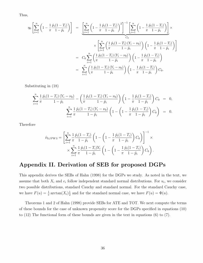
Thus,
η0
[n∑i=1
(1− 1
π
pi(1− Ti)1− pi
)]=
[n∑i=1
(1− 1
π
pi(1− Ti)1− pi
)2]−1 [ n∑
i=1
(1− 1
π
pi(1− Ti)1− pi
)]︸ ︷︷ ︸×
C0
×
[n∑i=1
(1π
pi(1− Ti) (Yi − ν0)1− pi
)(1− 1
π
pi(1− Ti)1− pi
)]
= C0
n∑i=1
(1π
pi(1− Ti) (Yi − ν0)1− pi
)(1− 1
π
pi(1− Ti)1− pi
)
=n∑i=1
(1π
pi(1− Ti) (Yi − ν0)1− pi
)(1− 1
π
pi(1− Ti)1− pi
)C0.
Substituting in (18)
n∑i=1
1
π
pi(1− Ti) (Yi − ν0)
1− pi−(
1
π
pi(1− Ti) (Yi − ν0)
1− pi
)(1− 1
π
pi(1− Ti)1− pi
)C0 = 0,
n∑i=1
1
π
pi(1− Ti) (Yi − ν0)
1− pi
(1−
(1− 1
π
pi(1− Ti)1− pi
)C0
)= 0.
Therefore
ν0,IPW3 =
[n∑i=1
1
π
pi(1− Ti)1− pi
(1−
(1− 1
π
pi(1− Ti)1− pi
)C0
)]−1
×
×n∑i=1
1
π
pi(1− Ti)Yi1− pi
(1−
(1− 1
π
pi(1− Ti)1− pi
)C0
).
Appendix II. Derivation of SEB for proposed DGPs
This appendix derives the SEBs of Hahn (1998) for the DGPs we study. As noted in the text, we
assume that both Xi and ei follow independent standard normal distributions. For ui, we consider
two possible distributions, standard Cauchy and standard normal. For the standard Cauchy case,
we have F (u) = 1π
arctan(Xi)12
and for the standard normal case, we have F (u) = Φ(u).
Theorems 1 and 2 of Hahn (1998) provide SEBs for ATE and TOT. We next compute the terms
of these bounds for the case of unknown propensity score for the DGPs specified in equations (10)
to (12) The functional form of these bounds are given in the text in equations (6) to (7).
36

Let σ2 denote the variance of ei. Then we have
Y 1i = β + (γ + δ)m(p(Xi)) + (1 + ψp(Xi)) ei,
E[Y 1i
∣∣Xi
]= β + (γ + δ)m(p(Xi)),
σ21(Xi) = E
[(Y 1i − E
[Y 1i |Xi
])2 ∣∣Xi
]= (1 + ψp(Xi))
2 σ2,
Y 0i = γm(p(Xi)) + (1− ψ(1− p(Xi)))ei,
E[Y 0i
∣∣Xi
]= γm(p(Xi)),
σ20(Xi) = E
[(Y 0i − E
[Y 0i |Xi
])2 ∣∣Xi
]= (1− ψ(1− p(Xi)))
2 σ2,
τ (Xi) = β + δm (p (Xi)) .
In order to compute the SEBs we need to find the expectation of the following functions:
1. Expressions involving the variance of the treated (first term of the SEB):
σ21(Xi)
p(Xi)=
(1 + ψp(Xi))2 σ2
p(Xi)= σ2
(1
p(Xi)+ 2ψ + ψ2p (Xi)
),
σ21(Xi)p(Xi) = (1 + ψp(Xi))
2 σ2p (Xi) = σ2(ψ2p (Xi)
3 + 2ψp(Xi)2 + p (Xi)
).
2. Expressions involving the variance of the controls (second term of the SEB)
σ20(Xi)
1− p(Xi)= σ2 (1− ψ(1− p(Xi)))
2
1− p(Xi)
= σ2
(1
1− p(Xi)+ ψ2(1− p(Xi))− 2ψ
),
σ20(Xi)p(Xi)
2
1− p(Xi)= σ2 (1− ψ(1− p(Xi)))
2 p(Xi)2
1− p(Xi)
= σ2
(p(Xi)
2
1− p(Xi)+ ψ2(1− p(Xi))p(Xi)
2 − 2ψp(Xi)2
).
3. Thus the first 2 terms of the ATE and the TOT are
σ21(Xi)
p(Xi)+
σ20(Xi)
1− p(Xi)= σ2
(1
p (Xi)+
1
1− p (Xi)+ ψ2
),
σ21(Xi)p(Xi) +
σ20(Xi)p(Xi)
2
(1− p(Xi))= σ2
(p (Xi) +
p (Xi)2
1− p (Xi)+ ψ2p (Xi) .
2
)
37

4. Expressions capturing the heterogeneity of the treatment (third term of the SEB)
(τ(Xi)− α)2 = (β − α)2 + δ2 [m (p (Xi))]2 +
+2 (β − α) δm (p (Xi)) ,
p(Xi)(τ(Xi)− θ)2 = (β − θ)2 p (Xi) + δ2 [m (p (Xi))]2 p (Xi) +
+2 (β − θ) δm (p (Xi)) p (Xi) ,
p(Xi)2(τ(Xi)− θ)2 = (β − θ)2 p (Xi)
2 + δ2 [m (p (Xi))]2 p (Xi)
2 +
+2 (β − θ) δm (p (Xi)) p (Xi)2 .
Therefore computation of the SEB involves computation of the integrals
1. For k = −1, 1, 2
A1 (k) = E[p (Xi)
k]
=
∫ ∞−∞
[Fu (η + κXi)]k fX (x) dx.
2. For k = 0, 2
A2 (k) = E
[p (Xi)
k
1− p (Xi)
]=
∫ ∞−∞
[Fu (η + κXi)]k
1− Fu (η + κXi)fX (x) dx.
3. For h = 1, 2 ; k = 0, 1, 2 ; j = 1, 2
A3 (h, k) = E[mj (p (Xi))
h p (Xi)k]
=
∫ ∞−∞
[mj (Fu (η + κXi))
h]h
[Fu (η + κXi)]k fX (x) dx.
Aside from A1(−1) and A2(0), these integrals are readily computed using mathematical software or
simulation. In the case where ui is distributed standard normal and κ is close to 1, the 2 integrals
listed are highly difficult to compute with any accuracy. For this case, we use an approach suggested
to us by Matias Cattaneo. Consider A1(−1) and A2 (0) in the case with ui distributed standard
normal. We have, for c = 1/|κ| > 1,
E
[1
p(Xi)
]=
∫ ∞−∞
φ(x)
Φ(η + κx)dx = c
∫ 0
−∞
φ(c(t− η))
Φ(t)dt+ c
∫ ∞0
φ(c(t− η))
Φ(t)dt
= c
∫ ∞0
φ(c(t+ η))
1− Φ(t)dt+ c
∫ ∞0
φ(c(t− η))
Φ(t)dt (21)
E
[1
1− p(Xi)
]=
∫ ∞−∞
φ(x)
1− Φ(η + κx)dx = c
∫ ∞0
φ(c(t− η))
1− Φ(t)dt+ c
∫ 0
−∞
φ(c(t− η))
1− Φ(t)dt
= c
∫ ∞0
φ(c(t− η))
1− Φ(t)dt+ c
∫ ∞0
φ(c(t+ η))
Φ(t)dt. (22)
The second integral in (21) and (22) is easy to simulate accurately because the numerator has
rapidly declining tails and the denominator is always between 0.5 and 1. The first integral in both
38
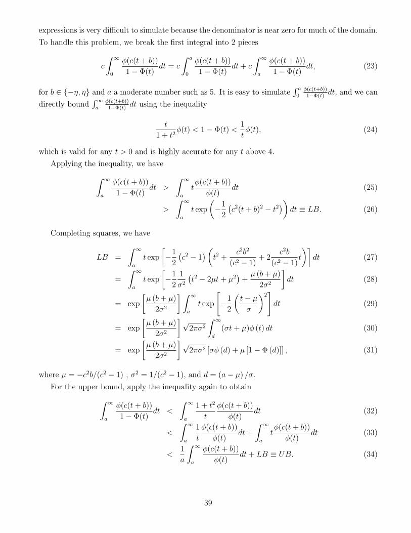
expressions is very difficult to simulate because the denominator is near zero for much of the domain.
To handle this problem, we break the first integral into 2 pieces
c
∫ ∞0
φ(c(t+ b))
1− Φ(t)dt = c
∫ a
0
φ(c(t+ b))
1− Φ(t)dt+ c
∫ ∞a
φ(c(t+ b))
1− Φ(t)dt, (23)
for b ∈ {−η, η} and a a moderate number such as 5. It is easy to simulate∫ a
0φ(c(t+b))1−Φ(t)
dt, and we can
directly bound∫∞a
φ(c(t+b))1−Φ(t)
dt using the inequality
t
1 + t2φ(t) < 1− Φ(t) <
1
tφ(t), (24)
which is valid for any t > 0 and is highly accurate for any t above 4.
Applying the inequality, we have∫ ∞a
φ(c(t+ b))
1− Φ(t)dt >
∫ ∞a
tφ(c(t+ b))
φ(t)dt (25)
>
∫ ∞a
t exp
(−1
2
(c2(t+ b)2 − t2
))dt ≡ LB. (26)
Completing squares, we have
LB =
∫ ∞a
t exp
[−1
2
(c2 − 1
)(t2 +
c2b2
(c2 − 1)+ 2
c2b
(c2 − 1)t
)]dt (27)
=
∫ ∞a
t exp
[−1
2
1
σ2
(t2 − 2µt+ µ2
)+µ (b+ µ)
2σ2
]dt (28)
= exp
[µ (b+ µ)
2σ2
] ∫ ∞a
t exp
[−1
2
(t− µσ
)2]dt (29)
= exp
[µ (b+ µ)
2σ2
]√2πσ2
∫ ∞d
(σt+ µ)φ (t) dt (30)
= exp
[µ (b+ µ)
2σ2
]√2πσ2 [σφ (d) + µ [1− Φ (d)]] , (31)
where µ = −c2b/(c2 − 1) , σ2 = 1/(c2 − 1), and d = (a− µ) /σ.
For the upper bound, apply the inequality again to obtain∫ ∞a
φ(c(t+ b))
1− Φ(t)dt <
∫ ∞a
1 + t2
t
φ(c(t+ b))
φ(t)dt (32)
<
∫ ∞a
1
t
φ(c(t+ b))
φ(t)dt+
∫ ∞a
tφ(c(t+ b))
φ(t)dt (33)
<1
a
∫ ∞a
φ(c(t+ b))
φ(t)dt+ LB ≡ UB. (34)
39

It is easy to show that∫ ∞a
φ(c(t+ b))
φ(t)dt =
∫ ∞a
φ(c(t+ b))
φ(t)dt =
∫ ∞a
exp
(−1
2
(c2(t+ b)2 − t2
))dt (35)
= exp
[µ (b+ µ)
2σ2
]√2πσ2
∫ ∞a
exp
[−1
2
(t− µσ
)2]dt (36)
= exp
[µ (b+ µ)
2σ2
]√2πσ2 (1− Φ (d)) . (37)
In summary, we have
LB <
∫ ∞a
φ (c(t+ b))
1− Φ(t)dt < UB (38)
where,
LB = exp
[µ (b+ µ)
2σ2
]√2πσ2 [σφ (d) + µ [1− Φ (d)]] , (39)
UB = LB + exp
[µ (b+ µ)
2σ2
] √2πσ2
a(1− Φ (d)) , (40)
and
µ =−c2b
(c2 − 1); σ2 =
1
(c2 − 1); d =
a− µσ
; c =1
κ; b ∈ {−η, η} . (41)
For example, for η = −0.3, κ = 0.8 and a = 7 the lower bound for this integral is 0.0000515 and
the upper bound is 0.0000526. For η = 0, κ = 0.95 and a = 7 the lower bound is 0.656062 and the
upper bound is 0.667721.
Appendix Figure 1 graphs the upper and lower bounds on the integral above, for η = 0, a = 7,
and κ ranging from 0.9 to 0.999. This graph makes two points. First, the bounds are extremely
accurate globally in κ. Second, the integral in question is an amazingly convex function of κ. Highly
similar patterns hold for other values of η.
40

References
Abadie, Alberto and Guido W. Imbens, “Large Sample Properties of Matching Estimators for
Average Treatment Effects,” Econometrica, January 2006, 74 (1), 235–267.
and , “On the Failure of the Bootstrap for Matching Estimators,” Econometrica, forth-
coming 2008.
Black, Dan A. and Jeffrey A. Smith, “How Robust is the Evidence on the Effects of College Quality?
Evidence From Matching,” Journal of Econometrics, July-August 2004, 121 (1-2), 99–124.
Blinder, Alan S., “Wage Discrimination: Reduced Form and Structural Estimates,” Journal of
Human Resources, Fall 1973, 8, 436–455.
Card, David, “The Effect of Unions on the Structure of Wages: A Longitudinal Analysis,” Econo-
metrica, 1996, 64, 957–979.
Card, David E., “The Causal Effect of Education on Earnings,” in Orley Ashenfelter and David E.
Card, eds., The Handbook of Labor Economics, Vol. 3A, Amsterdam: Elsevier, 1999.
Chen, Xiaohong, Han Hong, and Alessandro Tarozzi, “Semiparametric Efficiency in GMM Models
with Auxiliary Data,” Annals of Statistics, forthcoming 2008.
Crump, Richard K., V. Joseph Hotz, Guido W. Imbens, and Oscar A. Mitnik, “Dealing with Limited
Overlap in Estimation of Average Treatment Effects,” Unpublished manuscript, UCLA 2007.
, , , and , “Nonparametric Tests for Treatment Effect Heterogeneity,” Review
of Economics and Statistics, forthcoming 2007.
Deaton, Angus, The Analysis of Household Surveys : A Microeconomic Approach to Development
Policy, Washington, D.C.: World Bank, 1997.
Dehejia, Rajeev H. and Sadek Wahba, “Causal Effects in Non-Experimental Studies: Re-Evaluating
the Evaluation of Training Programs,” in “Econometric Methods for Program Evaluation,”
Cambridge: Rajeev H. Dehejia, Ph.D. Dissertation, Harvard University, 1997, chapter 1.
and , “Causal Effects in Nonexperimental Studies: Reevaluating the Evaluation of
Training Programs,” Journal of the American Statistical Association, December 1999, 94 (448),
1053–1062.
DiNardo, John E., Nicole M. Fortin, and Thomas Lemieux, “Labor Market Institutions and the
Distribution of Wages, 1973-1992: A Semiparametric Approach,” Econometrica, September
1996, 64 (5), 1001–1044.
41

Fan, Jianqing, “Local Linear Regression Smoothers and Their Minimax Efficiencies,” Annals of
Statistics, March 1993, 21 (1), 196–216.
Freedman, David A. and Richard A. Berk, “Weighting Regressions by Propensity Scores,” Evalu-
ation Review, 2008, 32 (4), 392–409.
Frolich, Markus, “Finite-Sample Properties of Propensity-Score Matching and Weighting Estima-
tors,” Review of Economics and Statistics, February 2004, 86 (1), 77–90.
Galdo, Jose, Jeffrey A. Smith, and Dan Black, “Bandwidth Selection and the Estimation of Treat-
ment Effects with Unbalanced Data,” Unpublished manuscript, University of Michigan 2007.
Hahn, Jinyong, “On the Role of the Propensity Score in Efficient Semiparametric Estimation of
Average Treatment Effects,” Econometrica, March 1998, 66 (2), 315–331.
Haviland, Amelia M. and Daniel S. Nagin, “Causal Inferences with Group Based Trajectory Mod-
els,” Psychometrika, September 2005, 70 (3), 1–22.
Heckman, James J. and Edward Vytlacil, “Structural Equations, Treatment Effects, and Econo-
metric Policy Evaluation,” Econometrica, 2005, 73 (3), 669–738.
and R. Robb, “Alternative Methods for Evaluating the Impact of Interventions,” in James J.
Heckman and R. Singer, eds., Longitudinal Analysis of Labor Market Data, Cambridge Uni-
versity Press Cambridge 1985.
, Hidehiko Ichimura, and Petra Todd, “Matching as an Econometric Evaluation Estimator:
Evidence from Evaluating a Job Training Programme,” Review of Economic Studies, October
1997, 64 (4), 605–654.
, , and , “Matching as an Econometric Evaluation Estimator,” Review of Economic
Studies, April 1998, 65 (2), 261–294.
, , Jeffrey Smith, and Petra Todd, “Characterizing Selection Bias Using Experimental
Data,” Econometrica, September 1998, 66 (5), 1017–1098.
, Sergio Urzua, and Edward Vytlacil, “Understanding Instrumental Variables in Models with
Essential Heterogeneity,” Review of Economics and Statistics, August 2006, 88 (3), 389–432.
Hirano, Keisuke, Guido W. Imbens, and Geert Ridder, “Efficient Estimation of Average Treatment
Effects Using the Estimated Propensity Score,” Econometrica, July 2003, 71 (4), 1161–1189.
Ho, Daniel, Kosuke Imai, Gary King, and Elizabeth Stuart, “Matching as Nonparametric Prepro-
cessing for Reducing Model Dependence in Parametric Causal Inference,” Political Analysis,
August 2007, 15, 199–236.
42

Horvitz, D. and D. Thompson, “A Generalization of Sampling Without Replacement from a Finite
Population,” Journal of the American Statistical Association, 1952, 47, 663–685.
Imbens, Guido W., “Nonparametric Estimation of Average Treatment Effects Under Exogeneity:
A Review,” Review of Economics and Statistics, February 2004, 86 (1), 4–29.
Johnston, Jack and John E. DiNardo, Econometric Methods, McGraw-Hill, 1996.
Katz, Lawrence F., Jeffrey R. Kling, and Jeffrey B. Liebman, “Moving to Opportunity in Boston:
Early Results of a Randomized Mobility Experiment,” Quarterly Journal of Economics, May
2001, 116 (2), 607–654.
Kent, David and Rodney Hayward, “Subgroup analyses in clinical trials.,” New England Journal
of Medicine, Mar 2008, 358 (11), 1199.
Khan, Shakeeb and Elie Tamer, “Irregular Identification, Support Conditions, and Inverse Weight
Estimation,” Unpublished manuscript, Northwestern University 2007.
Lechner, Michael, “A Note on the Common Support Problem in Applied Evaluation Studies,”
Discussion Paper N2001-01, Universitat St. Gallen 2001.
, “A Note on Endogenous Control Variables in Evaluation Studies,” Discussion Paper N2005-
16, Universitat St. Gallen 2005.
Loader, Clive R., “Bandwidth Selection: Classical or Plug-In?,” The Annals of Statistics, Apr
1999, 27 (2), 415–438.
Lunceford, Jared K. and Marie Davidian, “Stratification and Weighting via the Propensity Score
in Estimation of Causal Treatment Effects: A Comparative Study,” Statistics in Medicine, 15
October 2004, 23 (19), 2937–2960.
McCrary, Justin, “The Effect of Court-Ordered Hiring Quotas on the Composition and Quality of
Police,” American Economic Review, March 2007, 97 (4), 318–353.
, “Manipulation of the Running Variable in the Regression Discontinuity Design: A Density
Test,” Journal of Econometrics, February 2008, 142 (2).
Muirhead, Robb J., Aspects of Multivariate Statistical Theory, Hoboken: John Wiley and Sons,
2005.
Newey, Whitney, “Semiparametric Efficiency Bounds,” Journal of Applied Econometrics, April-
June 1990, 5 (2), 99–135.
Oaxaca, Ronald, “Male–Female Wage Differentials in Urban Labor Markets,” International Eco-
nomic Review, 1973, 14, 693–709.
43

Robins, James M. and Andrea Rotnitzky, “Semiparametric Efficiency in Multivariate Regression
Models With Missing Data,” Journal of the American Statistical Association, March 1995, 90
(429), 122–129.
, , and Lue Ping Zhao, “Estimation of Regression Coefficients When Some Regressors
Are Not Always Observed,” Journal of the American Statistical Association, September 1994,
89 (427), 846–866.
Rosenbaum, Paul R. and Donald B. Rubin, “The Central Role of the Propensity Score in Obser-
vational Studies for Causal Effects,” Biometrika, April 1983, 70 (1), 41–55.
Ruud, Paul A., An Introduction to Classical Econometric Theory, New York: Oxford University
Press, 2000.
Seifert, Burkhardt and Theo Gasser, “Data Adaptive Ridging in Local Polynomial Regression,”
Journal of Computational and Graphical Statistics, June 2000, 9 (2), 338–360.
Smith, Jeffrey A. and Petra Todd, “Does Matching Overcome Lalonde’s Critique of Nonexperi-
mental Estimators?,” Journal of Econometrics, September 2005, 125 (1–2), 305–353.
Stone, Mervyn, “Cross-Validatory Choice and Assessment of Statistical Predictions,” Journal of
the Royal Statistical Society, Series B, 1974, 36 (2), 111–147.
Todd, Petra, “Matching Estimators,” in P. Newman, M. Milgate, and J. Eatwell, eds., The New
Palgrave—A Dictionary of Economics, Vol. forthcoming, New York: Macmillan, 2007.
Wishart, John, “The Generalised Product Moment Distribution in Samples from a Normal Multi-
variate Population,” Biometrika, July 1928, 20A (1/2), 32–52.
Wooldridge, Jeffrey M., Econometric Analysis of Cross Section and Panel Data, Cambridge: MIT
Press, 2002.
Zhao, Zong, “Using Matching to Estimate Treatment Effects: Data Requirements, Matching Met-
rics, and Monte Carlo Evidence,” Review of Economics and Statistics, February 2004, 86 (1),
91–107.
, “Sensitivity of Propensity Score Method to the Specifications,” Economics Letters, 2008, 98,
309–319.
44

Figure 1.A: Overlap Plots, by design (Normal-Cauchy model)
0.2 0.4 0.6 0.8 1.0
0.5
1.0
1.5
2.0
Conditional pdfs of pHXL: h=0 ; k=0.8
0.2 0.4 0.6 0.8 1.0
1
2
3
4
Conditional pdfs of pHXL: h=0.8 ; k=1
0.2 0.4 0.6 0.8 1.0
1
2
3
4
Conditional pdfs of pHXL: h=-0.8 ; k=1
f p|D=0 f p|D=1
Figure 1.B: Overlap Plots, by design (Normal-Normal model)
0.2 0.4 0.6 0.8 1.0
0.5
1.0
1.5
Conditional pdfs of pHXL: h=0 ; k=0.95
0.2 0.4 0.6 0.8 1.0
0.5
1.0
1.5
2.0Conditional pdfs of pHXL: h=0.3 ; k=-0.8
0.2 0.4 0.6 0.8 1.0
0.5
1.0
1.5
2.0Conditional pdfs of pHXL: h=-0.3 ; k=0.8
f p|D=0 f p|D=1
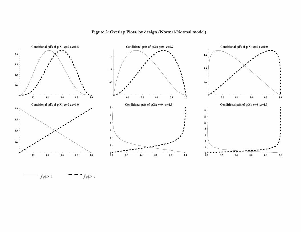
Figure 2: Overlap Plots, by design (Normal-Normal model)
0.2 0.4 0.6 0.8 1.0
0.5
1.0
1.5
2.0
Conditional pdfs of pHXL: h=0 ; k=0.5
0.2 0.4 0.6 0.8 1.0
0.5
1.0
1.5
Conditional pdfs of pHXL: h=0 ; k=0.7
0.2 0.4 0.6 0.8 1.0
0.5
1.0
1.5
Conditional pdfs of pHXL: h=0 ; k=0.9
0.2 0.4 0.6 0.8 1.0
0.5
1.0
1.5
2.0Conditional pdfs of pHXL: h=0 ; k=1.0
0.0 0.2 0.4 0.6 0.8 1.00
1
2
3
4
5
6Conditional pdfs of pHXL: h=0 ; k=1.3
0.0 0.2 0.4 0.6 0.8 1.00
2
4
6
8
10
12
14
Conditional pdfs of pHXL: h=0 ; k=1.5
f p|D=0 f p|D=1

47

48

Sample Size SettingPair
matchBlocking k-NN
Kernel match (Epa)
Kernel match
(Gauss)
LLR match (Epa)
LLR match
(Gauss)
Ridge match (Epa)
Ridge match
(Gauss)IPW1 IPW2 IPW3
Double robust
Control function
A. Simulated Root 100 I. Homog.-Homosk. 5.2 25.1* 42.5* 35.5* 39.5* 39.0* 39.5* 9.2* 12.8* 3.2 4.0 4.9* 2.5 3.0 Mean Squared Bias II. Heterog.-Homosk. 2.8 44.4* 41.9* 34.9* 39.2* 38.4* 39.3* 7.8* 12.0* 1.4 2.4 3.1 5.0* 2.0 (x 1000) III. Homog.-Heterosk. 5.0 26.9* 35.3* 26.8* 28.6* 11.2* 13.0* 8.5* 10.7* 3.5 4.1 4.8 4.1 3.8
IV. Heterog.-Heterosk. 3.3 42.6* 34.0* 25.0* 26.9* 10.9* 13.2* 6.1* 8.3* 2.2 2.1 2.5 6.5* 2.3
All 4.2 35.8* 38.6* 30.9* 34.0* 28.5* 29.4* 8.0* 11.1* 2.7 3.3 4.0* 4.8* 2.9F-stat (no bias) 37.7 3505.5 5276.1 3309.3 4163.6 2144.7 2384.1 183.4 379.0 19.3 30.9 46.0 58.5 18.8[p-value] [0.037] [0.000] [0.000] [0.000] [0.000] [0.000] [0.000] [0.000] [0.000] [0.734] [0.155] [0.004] [0.000] [0.760]
500 I. Homog.-Homosk. 2.4 7.6* 36.0* 30.2* 33.4* 2.9 2.9 3.1 4.9* 2.3 2.3 2.2 1.9 1.7II. Heterog.-Homosk. 2.2 7.7* 32.9* 27.8* 31.1* 2.1 1.8 1.7 2.9 1.9 1.9 1.8 2.6 2.0III. Homog.-Heterosk. 2.4 6.8* 23.2* 16.2* 17.9* 2.4 2.4 2.6 3.2 2.3 2.3 2.2 2.3 2.4IV. Heterog.-Heterosk. 2.3 9.8* 25.0* 17.5* 19.4* 2.4 2.7 3.2 4.3 2.2 2.2 2.4 1.6 2.2
All 2.3 8.0* 29.8* 23.7* 26.4* 2.5 2.5 2.7 3.9* 2.2 2.2 2.2 2.2 2.1F-stat (no bias) 12.1 182.4 3094.5 2043.2 2548.8 17.6 18.1 20.6 45.8 13.7 13.9 13.5 14.0 11.9[p-value] [0.979] [0.000] [0.000] [0.000] [0.000] [0.824] [0.800] [0.662] [0.005] [0.953] [0.949] [0.958] [0.946] [0.981]
B. Simulated 100 I. Homog.-Homosk. 103.3* 68.9* 53.5* 56.2* 54.5* 82.4* 78.5* 67.4* 64.0* 72.2* 65.8* 65.5* 65.8* 89.3* Average Variance II. Heterog.-Homosk. 106.2* 74.9* 54.9* 57.6* 55.7* 84.1* 80.0* 68.9* 65.4* 73.0* 66.9* 66.8* 67.2* 91.4* (x 1000) III. Homog.-Heterosk. 119.0* 110.1* 108.0 109.0 108.8 113.7* 113.0* 111.7 111.1 118.4* 112.6* 112.0* 117.6* 115.9*
IV. Heterog.-Heterosk. 118.1* 113.7* 107.0* 107.8* 107.6* 112.9* 112.1 110.5 110.0 117.6* 111.7 110.9 117.0* 115.5*
Average (V-SEB)/SEB 0.376 0.083 -0.078 -0.052 -0.067 0.180 0.145 0.050 0.020 0.116 0.040 0.035 0.064 0.247F-stat (V = SEB) 418.6 45.4 73.0 30.1 54.5 158.5 116.4 17.5 4.0 60.1 9.7 8.3 19.5 243.7[p-value] [0.000] [0.000] [0.000] [0.000] [0.000] [0.000] [0.000] [0.000] [0.000] [0.000] [0.000] [0.000] [0.000] [0.000]
500 I. Homog.-Homosk. 21.1* 12.8 11.2* 11.2* 11.1* 13.5* 12.9 13.0 12.6 13.3* 12.6 12.6 12.6 12.9II. Heterog.-Homosk. 21.5* 13.3* 11.6* 11.4* 11.3* 13.6* 13.2* 13.2* 12.8 13.7* 12.9 12.9 13.0 13.3*III. Homog.-Heterosk. 24.1* 21.8 21.2 21.5 21.5 22.2 22.0 22.0 21.8 22.6 21.9 21.8 21.9 21.9IV. Heterog.-Heterosk. 24.1* 22.3 21.5 21.8 21.8 22.5 22.3 22.3 22.2 23.0 22.3 22.2 22.4 22.3
Average (V-SEB)/SEB 0.398 0.021 -0.060 -0.055 -0.062 0.048 0.025 0.027 0.009 0.059 0.012 0.010 0.014 0.025F-stat (V = SEB) 88.8 1.6 11.3 9.5 12.3 3.3 1.4 1.5 0.7 3.9 0.8 0.7 0.9 1.6[p-value] [0.000] [0.032] [0.000] [0.000] [0.000] [0.000] [0.097] [0.064] [0.817] [0.000] [0.793] [0.817] [0.584] [0.032]
Table 1: Bias and Variance of the Estimated Treatment Effect on the Treated (TOT)Normal-Cauchy Model
NOTES: Replications: 10,000 for N=100 and 2000 for N=500. Estimators: See sections II.B and II.C. The numbers of neighbors in k-NN and the bandwidth of kernel-based matching were selected using leave-one-out cross validation (see section II.D). Models: Normal-Cauchy uses a treatment equation with a Cauchy distributed error term. Normal-Normal has an error term which is standard Normal. (see section III andsection IV). Settings: Simulations were done for 24 different contexts which combine two outcome curves, three treatment designs, and four settings (homogeneous treatment - homoskedastic outcome error,homogenous-heteroskedastic, etc.) See section III and section IV.
Statistics (RMSB, AV and SEB): We summarize results by showing simulated root mean square bias (RMSB) and the average variance (AV) for each setting. For a given setting, RMSB=sqrt{(1/6)(b1+...+b6)} andthe AV=(1/6)(v1+…+v6) where bi (i=1,…,6) is the square of the bias and vi (i=1,…,6) is the variance of one of the six combinations of the two curves and the three designs. “All” is the RMSB across all 24contexts. Average (V-SEB)/SEB is the average percentage difference between the variance and the semiparametric efficiency bound (SEB). See section II.E and Appendix II. Stars, tests and p-values: We presenttwo F-tests and their p-values: (i) H0:bias=0, (ii) H0: V=SEB (see section IV for details). One star means that we reject the null at the 1%.

Misspec. Type
SettingPair
matchBlocking k-NN
Kernel match (Epa)
Kernel match
(Gauss)
LLR match (Epa)
LLR match
(Gauss)
Ridge match (Epa)
Ridge match
(Gauss)IPW1 IPW2 IPW3
Double robust
Control function
A. Simulated Root Xs I. Homog.-Homosk. 127.2* 123.2* 142.4* 141.1* 142.6* 155.4* 153.3* 128.7* 130.4* 125.4* 125.6* 125.9* 125.2* 124.9* Mean Squared Bias II. Heterog.-Homosk. 126.4* 120.9* 143.1* 141.6* 143.1* 156.3* 154.0* 128.8* 130.5* 125.3* 125.7* 126.2* 123.7* 125.1* (x 1000) III. Homog.-Heterosk. 125.5* 122.7* 140.8* 139.3* 140.6* 131.4* 132.3* 127.7* 129.4* 124.6* 124.9* 125.2* 124.5* 124.2*
IV. Heterog.-Heterosk. 126.1* 120.1* 142.2* 140.7* 142.1* 131.8* 132.8* 128.4* 130.4* 125.5* 125.9* 126.2* 123.2* 124.9*
All 126.3* 121.7* 142.1* 140.7* 142.1* 144.2* 143.5* 128.4* 130.2* 125.2* 125.5* 125.9* 124.1* 124.8*F-stat (no bias) 36397.5 46067.5 69490.6 67500.6 70217.2 56723.0 58158.0 51241.9 54298.3 49436.3 50884.0 51261.2 48656.0 43699.7[p-value] [0.000] [0.000] [0.000] [0.000] [0.000] [0.000] [0.000] [0.000] [0.000] [0.000] [0.000] [0.000] [0.000] [0.000]
Dist of u. I. Homog.-Homosk. 5.4 27.3* 42.6* 37.0* 40.7* 39.5* 41.1* 9.5* 12.9* 22.6* 7.6* 6.5* 2.4 2.1II. Heterog.-Homosk. 3.0 47.3* 42.3* 36.3* 40.1* 39.1* 40.3* 8.4* 12.1* 19.5* 4.7* 3.9 7.3* 4.0III. Homog.-Heterosk. 5.4 28.7* 36.1* 29.4* 31.8* 12.8* 15.5* 9.3* 11.5* 21.8* 7.9* 7.1* 4.0 3.8IV. Heterog.-Heterosk. 3.6 46.1* 34.7* 27.9* 30.3* 12.7* 15.8* 7.1* 9.2* 21.0* 7.9* 6.1* 8.6* 3.1
All 4.5 38.5* 39.1* 32.9* 36.0* 29.2* 30.8* 8.6* 11.5* 21.3* 7.2* 6.0* 6.1* 3.3F-stat (no bias) 42.4 4067.8 5378.4 3728.1 4597.8 2209.3 2587.9 212.0 402.1 744.2 130.1 98.5 99.0 23.8[p-value] [0.012] [0.000] [0.000] [0.000] [0.000] [0.000] [0.000] [0.000] [0.000] [0.000] [0.000] [0.000] [0.000] [0.474]
B. Simulated Xs I. Homog.-Homosk. 87.4* 55.0* 48.3* 48.8* 47.7* 67.2* 64.3* 55.8* 53.6* 54.9* 53.0* 52.9* 53.8* 64.9* Average Variance II. Heterog.-Homosk. 88.0* 59.0* 49.9* 50.2* 49.1* 68.8* 65.6* 57.0* 54.8* 56.0* 54.3* 54.2* 55.0* 66.3* (x 1000) III. Homog.-Heterosk. 132.7* 121.7* 121.4* 121.5* 121.3* 125.5* 124.8* 123.2* 122.5* 124.4* 122.6* 122.5* 128.3* 126.3*
IV. Heterog.-Heterosk. 132.5* 124.6* 121.8* 121.9* 121.7* 125.6* 125.2* 123.5* 123.0* 124.4* 122.9* 122.8* 128.7* 126.6*
Average (V-SEB)/SEB -0.066 -0.266 -0.314 -0.311 -0.318 -0.197 -0.216 -0.268 -0.282 -0.270 -0.285 -0.286 -0.261 -0.208F-stat (V = SEB) 36.0 1079.7 2031.3 1955.7 2150.8 460.2 580.3 1095.5 1323.2 1186.4 1387.9 1401.2 1258.8 512.1[p-value] [0.000] [0.000] [0.000] [0.000] [0.000] [0.000] [0.000] [0.000] [0.000] [0.000] [0.000] [0.000] [0.000] [0.000]
Dist of u. I. Homog.-Homosk. 103.1* 68.6* 53.1* 55.4* 53.9* 82.9* 78.9* 67.2* 63.8* 93.3* 72.2* 67.3* 68.5* 93.0*II. Heterog.-Homosk. 105.9* 74.9* 54.5* 56.7* 55.1* 84.1* 80.0* 68.5* 65.3* 93.8* 73.3* 68.9* 70.1* 96.5*III. Homog.-Heterosk. 118.7* 110.2* 107.5* 108.8 108.7 114.1* 113.9* 111.7* 111.2 138.9* 118.7* 114.8* 121.4* 118.7*IV. Heterog.-Heterosk. 117.8* 114.4* 106.4* 107.7* 107.4* 113.4* 113.0* 110.6 110.1 145.4* 118.5* 114.0* 121.4* 117.6*
Average (V-SEB)/SEB 0.373 0.084 -0.084 -0.060 -0.073 0.184 0.150 0.047 0.019 0.383 0.118 0.063 0.105 0.293F-stat (V = SEB) 415.7 46.4 77.1 40.0 62.1 162.5 119.1 16.1 3.5 418.4 80.3 27.9 61.0 296.0[p-value] [0.000] [0.000] [0.000] [0.000] [0.000] [0.000] [0.000] [0.000] [0.000] [0.000] [0.000] [0.000] [0.000] [0.000]
Table 2: Bias and Variance of the Estimated Treatment Effect on the Treated (TOT) under MisspecificationMisspecification of the Propensity Score in the Normal-Cauchy Model (sample size 100)
NOTES: Replications: 10,000 for N=100 and 2000 for N=500. Estimators: See sections II.B and II.C. The numbers of neighbors in k-NN and the bandwidth of kernel-based matching were selected using leave-one-out cross validation (see section II.D). Models: Normal-Cauchy uses a treatment equation with a Cauchy distributed error term. Normal-Normal has an error term which is standard Normal. (see section III andsection IV). Settings: Simulations were done for 24 different contexts which combine two outcome curves, three treatment designs, and four settings (homogeneous treatment - homoskedastic outcome error,homogenous-heteroskedastic, etc.) See section III and section IV.
Statistics (RMSB, AV and SEB): We summarize results by showing simulated root mean square bias (RMSB) and the average variance (AV) for each setting. For a given setting, RMSB=sqrt{(1/6)(b1+...+b6)} andthe AV=(1/6)(v1+…+v6) where bi (i=1,…,6) is the square of the bias and vi (i=1,…,6) is the variance of one of the six combinations of the two curves and the three designs. “All” is the RMSB across all 24contexts. Average (V-SEB)/SEB is the average percentage difference between the variance and the semiparametric efficiency bound (SEB). See section II.E and Appendix II. Stars, tests and p-values: We presenttwo F-tests and their p-values: (i) H0:bias=0, (ii) H0: V=SEB (see section IV for details). One star means that we reject the null at the 1%.

N SettingPair
matchBlocking k-NN
Kernel match (Epa)
Kernel match
(Gauss)
LLR match (Epa)
LLR match
(Gauss)
Ridge match (Epa)
Ridge match
(Gauss)IPW1 IPW2 IPW3
Double robust
Control function
A. Simulated Root 100 I. Homog.-Homosk. 19.3* 45.1* 88.8* 70.5* 76.7* 54.2* 55.4* 26.9* 32.1* 15.8* 16.7* 16.8* 3.3 7.8* Mean Squared Bias II. Heterog.-Homosk. 16.5* 66.3* 87.4* 68.6* 75.1* 53.3* 55.0* 25.4* 30.4* 12.8* 14.8* 15.4* 16.9* 7.6* (x 1000) III. Homog.-Heterosk. 14.4* 43.4* 76.1* 55.4* 58.7* 21.6* 25.4* 24.4* 27.5* 15.2* 13.8* 13.9* 3.7 6.6
IV. Heterog.-Heterosk. 14.6* 67.4* 74.8* 54.2* 57.9* 21.1* 24.3* 23.0* 26.7* 15.0* 12.4* 12.9* 19.5* 5.7
All 16.3* 56.7* 82.0* 62.6* 67.7* 40.9* 42.8* 24.9* 29.3* 14.7* 14.5* 14.8* 13.2* 7.0*F-stat (no bias) 428.2 6163.6 21354.4 11216.0 13439.8 3071.5 3564.4 1385.7 1989.8 267.3 422.9 466.7 335.6 69.9[p-value] [0.000] [0.000] [0.000] [0.000] [0.000] [0.000] [0.000] [0.000] [0.000] [0.000] [0.000] [0.000] [0.000] [0.000]
500 I. Homog.-Homosk. 7.8* 17.1* 72.1* 52.8* 58.4* 12.0* 14.2* 14.1* 17.4* 3.1 6.3 7.7* 4.0 6.4*II. Heterog.-Homosk. 5.9 16.4* 68.7* 50.1* 55.4* 9.8* 12.1* 11.5* 15.4* 4.7 4.1 4.5 8.5* 3.5III. Homog.-Heterosk. 4.1 15.0* 60.3* 36.9* 40.5* 7.3* 8.4* 11.0* 13.1* 4.4 3.8 5.4 2.7 3.5IV. Heterog.-Heterosk. 7.3 17.4* 60.7* 37.2* 40.7* 9.6* 9.9* 12.2* 14.1* 4.6 6.7 7.5* 6.4 5.0
All 6.4* 16.5* 65.7* 44.9* 49.4* 9.8* 11.4* 12.3* 15.1* 4.3 5.4* 6.4* 5.8* 4.7F-stat (no bias) 52.8 487.7 12564.8 5392.8 6719.7 167.8 251.3 285.5 461.6 23.6 43.6 71.8 68.1 42.0[p-value] [0.001] [0.000] [0.000] [0.000] [0.000] [0.000] [0.000] [0.000] [0.000] [0.482] [0.009] [0.000] [0.000] [0.013]
B. Simulated 100 I. Homog.-Homosk. 139.6* 104.8* 58.0* 66.5* 64.9* 117.1* 108.8* 88.7* 84.6* 166.8* 98.1* 93.1* 92.7* 166.2* Average Variance II. Heterog.-Homosk. 143.6* 122.1* 59.2* 68.5* 66.7* 119.0* 111.4* 91.4* 87.1* 162.3* 101.5* 96.0* 96.5* 169.4* (x 1000) III. Homog.-Heterosk. 152.0* 141.2* 120.1* 127.9* 128.1* 140.8* 139.3* 133.4* 133.0* 207.5* 149.1* 142.2* 152.8* 162.2*
IV. Heterog.-Heterosk. 151.7* 156.0* 120.0* 127.1* 126.8* 139.6* 138.6* 132.7* 132.1* 195.2* 149.0* 142.2* 153.6* 161.6*
Average (V-SEB)/SEB -0.280 -0.375 -0.570 -0.533 -0.537 -0.369 -0.392 -0.459 -0.472 -0.165 -0.404 -0.432 -0.410 -0.190F-stat (V = SEB) 6454.1 8872.2 46732.8 31680.5 33472.8 9986.0 11525.1 17199.1 18762.0 2701.3 11956.3 13919.1 12969.7 4169.5[p-value] [0.000] [0.000] [0.000] [0.000] [0.000] [0.000] [0.000] [0.000] [0.000] [0.000] [0.000] [0.000] [0.000] [0.000]
500 I. Homog.-Homosk. 33.7* 21.4* 13.2* 15.0* 14.6* 22.1* 20.2* 19.8* 18.7* 39.8* 24.5* 21.0* 21.4* 21.9*II. Heterog.-Homosk. 33.9* 22.8* 13.2* 14.9* 14.5* 22.0* 20.1* 19.7* 18.7* 36.3* 24.2* 20.8* 21.4* 21.6*III. Homog.-Heterosk. 35.7* 29.8* 24.2* 26.9* 26.8* 30.6* 29.8* 28.7* 28.4* 44.3* 34.4* 30.6* 31.7* 29.7*IV. Heterog.-Heterosk. 36.4* 30.8* 24.5* 27.1* 26.9* 30.9* 29.7* 28.9* 28.6* 86.9* 34.2* 30.7* 31.7* 29.7*
Average (V-SEB)/SEB -0.162 -0.379 -0.547 -0.503 -0.510 -0.375 -0.409 -0.423 -0.439 -0.011 -0.322 -0.393 -0.380 -0.387F-stat (V = SEB) 627.6 1754.0 7311.1 4590.5 4981.7 1688.7 2165.0 2390.6 2688.4 244.4 1087.3 1904.1 1704.4 1877.6[p-value] [0.000] [0.000] [0.000] [0.000] [0.000] [0.000] [0.000] [0.000] [0.000] [0.000] [0.000] [0.000] [0.000] [0.000]
NOTES: Replications: 10,000 for N=100 and 2000 for N=500. Estimators: See sections II.B and II.C. The numbers of neighbors in k-NN and the bandwidth of kernel-based matching were selected using leave-one-out cross validation (see section II.D). Models: Normal-Cauchy uses a treatment equation with a Cauchy distributed error term. Normal-Normal has an error term which is standard Normal. (see section III andsection IV). Settings: Simulations were done for 24 different contexts which combine two outcome curves, three treatment designs, and four settings (homogeneous treatment - homoskedastic outcome error,homogenous-heteroskedastic, etc.) See section III and section IV.
Statistics (RMSB, AV and SEB): We summarize results by showing simulated root mean square bias (RMSB) and the average variance (AV) for each setting. For a given setting, RMSB=sqrt{(1/6)(b1+...+b6)} andthe AV=(1/6)(v1+…+v6) where bi (i=1,…,6) is the square of the bias and vi (i=1,…,6) is the variance of one of the six combinations of the two curves and the three designs. “All” is the RMSB across all 24contexts. Average (V-SEB)/SEB is the average percentage difference between the variance and the semiparametric efficiency bound (SEB). See section II.E and Appendix II. Stars, tests and p-values: We presenttwo F-tests and their p-values: (i) H0:bias=0, (ii) H0: V=SEB (see section IV for details). One star means that we reject the null at the 1%.
Table 3: Bias and Variance of the Estimated Treatment Effect on the Treated (TOT)Normal-Normal Model
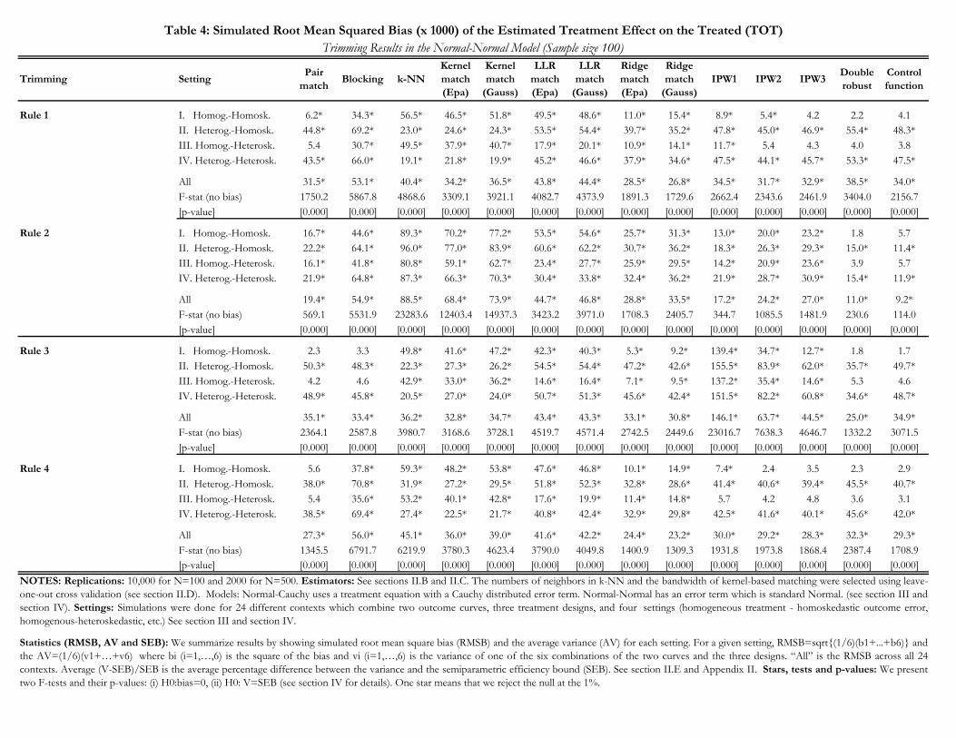
Trimming SettingPair
matchBlocking k-NN
Kernel match (Epa)
Kernel match
(Gauss)
LLR match (Epa)
LLR match
(Gauss)
Ridge match (Epa)
Ridge match
(Gauss)IPW1 IPW2 IPW3
Double robust
Control function
Rule 1 I. Homog.-Homosk. 6.2* 34.3* 56.5* 46.5* 51.8* 49.5* 48.6* 11.0* 15.4* 8.9* 5.4* 4.2 2.2 4.1II. Heterog.-Homosk. 44.8* 69.2* 23.0* 24.6* 24.3* 53.5* 54.4* 39.7* 35.2* 47.8* 45.0* 46.9* 55.4* 48.3*III. Homog.-Heterosk. 5.4 30.7* 49.5* 37.9* 40.7* 17.9* 20.1* 10.9* 14.1* 11.7* 5.4 4.3 4.0 3.8IV. Heterog.-Heterosk. 43.5* 66.0* 19.1* 21.8* 19.9* 45.2* 46.6* 37.9* 34.6* 47.5* 44.1* 45.7* 53.3* 47.5*
All 31.5* 53.1* 40.4* 34.2* 36.5* 43.8* 44.4* 28.5* 26.8* 34.5* 31.7* 32.9* 38.5* 34.0*F-stat (no bias) 1750.2 5867.8 4868.6 3309.1 3921.1 4082.7 4373.9 1891.3 1729.6 2662.4 2343.6 2461.9 3404.0 2156.7[p-value] [0.000] [0.000] [0.000] [0.000] [0.000] [0.000] [0.000] [0.000] [0.000] [0.000] [0.000] [0.000] [0.000] [0.000]
Rule 2 I. Homog.-Homosk. 16.7* 44.6* 89.3* 70.2* 77.2* 53.5* 54.6* 25.7* 31.3* 13.0* 20.0* 23.2* 1.8 5.7II. Heterog.-Homosk. 22.2* 64.1* 96.0* 77.0* 83.9* 60.6* 62.2* 30.7* 36.2* 18.3* 26.3* 29.3* 15.0* 11.4*III. Homog.-Heterosk. 16.1* 41.8* 80.8* 59.1* 62.7* 23.4* 27.7* 25.9* 29.5* 14.2* 20.9* 23.6* 3.9 5.7IV. Heterog.-Heterosk. 21.9* 64.8* 87.3* 66.3* 70.3* 30.4* 33.8* 32.4* 36.2* 21.9* 28.7* 30.9* 15.4* 11.9*
All 19.4* 54.9* 88.5* 68.4* 73.9* 44.7* 46.8* 28.8* 33.5* 17.2* 24.2* 27.0* 11.0* 9.2*F-stat (no bias) 569.1 5531.9 23283.6 12403.4 14937.3 3423.2 3971.0 1708.3 2405.7 344.7 1085.5 1481.9 230.6 114.0[p-value] [0.000] [0.000] [0.000] [0.000] [0.000] [0.000] [0.000] [0.000] [0.000] [0.000] [0.000] [0.000] [0.000] [0.000]
Rule 3 I. Homog.-Homosk. 2.3 3.3 49.8* 41.6* 47.2* 42.3* 40.3* 5.3* 9.2* 139.4* 34.7* 12.7* 1.8 1.7II. Heterog.-Homosk. 50.3* 48.3* 22.3* 27.3* 26.2* 54.5* 54.4* 47.2* 42.6* 155.5* 83.9* 62.0* 35.7* 49.7*III. Homog.-Heterosk. 4.2 4.6 42.9* 33.0* 36.2* 14.6* 16.4* 7.1* 9.5* 137.2* 35.4* 14.6* 5.3 4.6IV. Heterog.-Heterosk. 48.9* 45.8* 20.5* 27.0* 24.0* 50.7* 51.3* 45.6* 42.4* 151.5* 82.2* 60.8* 34.6* 48.7*
All 35.1* 33.4* 36.2* 32.8* 34.7* 43.4* 43.3* 33.1* 30.8* 146.1* 63.7* 44.5* 25.0* 34.9*F-stat (no bias) 2364.1 2587.8 3980.7 3168.6 3728.1 4519.7 4571.4 2742.5 2449.6 23016.7 7638.3 4646.7 1332.2 3071.5[p-value] [0.000] [0.000] [0.000] [0.000] [0.000] [0.000] [0.000] [0.000] [0.000] [0.000] [0.000] [0.000] [0.000] [0.000]
Rule 4 I. Homog.-Homosk. 5.6 37.8* 59.3* 48.2* 53.8* 47.6* 46.8* 10.1* 14.9* 7.4* 2.4 3.5 2.3 2.9II. Heterog.-Homosk. 38.0* 70.8* 31.9* 27.2* 29.5* 51.8* 52.3* 32.8* 28.6* 41.4* 40.6* 39.4* 45.5* 40.7*III. Homog.-Heterosk. 5.4 35.6* 53.2* 40.1* 42.8* 17.6* 19.9* 11.4* 14.8* 5.7 4.2 4.8 3.6 3.1IV. Heterog.-Heterosk. 38.5* 69.4* 27.4* 22.5* 21.7* 40.8* 42.4* 32.9* 29.8* 42.5* 41.6* 40.1* 45.6* 42.0*
All 27.3* 56.0* 45.1* 36.0* 39.0* 41.6* 42.2* 24.4* 23.2* 30.0* 29.2* 28.3* 32.3* 29.3*F-stat (no bias) 1345.5 6791.7 6219.9 3780.3 4623.4 3790.0 4049.8 1400.9 1309.3 1931.8 1973.8 1868.4 2387.4 1708.9[p-value] [0.000] [0.000] [0.000] [0.000] [0.000] [0.000] [0.000] [0.000] [0.000] [0.000] [0.000] [0.000] [0.000] [0.000]
NOTES: Replications: 10,000 for N=100 and 2000 for N=500. Estimators: See sections II.B and II.C. The numbers of neighbors in k-NN and the bandwidth of kernel-based matching were selected using leave-one-out cross validation (see section II.D). Models: Normal-Cauchy uses a treatment equation with a Cauchy distributed error term. Normal-Normal has an error term which is standard Normal. (see section III andsection IV). Settings: Simulations were done for 24 different contexts which combine two outcome curves, three treatment designs, and four settings (homogeneous treatment - homoskedastic outcome error,homogenous-heteroskedastic, etc.) See section III and section IV.
Statistics (RMSB, AV and SEB): We summarize results by showing simulated root mean square bias (RMSB) and the average variance (AV) for each setting. For a given setting, RMSB=sqrt{(1/6)(b1+...+b6)} andthe AV=(1/6)(v1+…+v6) where bi (i=1,…,6) is the square of the bias and vi (i=1,…,6) is the variance of one of the six combinations of the two curves and the three designs. “All” is the RMSB across all 24contexts. Average (V-SEB)/SEB is the average percentage difference between the variance and the semiparametric efficiency bound (SEB). See section II.E and Appendix II. Stars, tests and p-values: We presenttwo F-tests and their p-values: (i) H0:bias=0, (ii) H0: V=SEB (see section IV for details). One star means that we reject the null at the 1%.
Table 4: Simulated Root Mean Squared Bias (x 1000) of the Estimated Treatment Effect on the Treated (TOT)Trimming Results in the Normal-Normal Model (Sample size 100)

Trimming SettingPair
matchBlocking k-NN
Kernel match (Epa)
Kernel match
(Gauss)
LLR match (Epa)
LLR match
(Gauss)
Ridge match (Epa)
Ridge match
(Gauss)IPW1 IPW2 IPW3
Double robust
Control function
Rule 1 I. Homog.-Homosk. 125.7* 86.7* 61.1* 66.2* 63.5* 102.7* 97.6* 81.6* 77.4* 85.2* 79.0* 81.8* 79.5* 111.3*II. Heterog.-Homosk. 128.0* 99.6* 62.8* 67.7* 65.4* 105.2* 100.0* 83.9* 79.4* 87.3* 81.6* 84.2* 81.2* 114.0*III. Homog.-Heterosk. 141.9* 134.1* 127.2* 130.0* 130.1* 136.6* 136.1* 132.7* 132.3* 141.5* 134.9* 136.1* 143.1* 141.7*IV. Heterog.-Heterosk. 141.9* 144.5* 128.5* 130.9* 130.9* 137.0* 136.8* 133.6* 133.0* 142.9* 136.5* 137.2* 145.1* 141.6*
Average (V-SEB)/SEB -0.331 -0.441 -0.545 -0.526 -0.533 -0.411 -0.426 -0.476 -0.490 -0.451 -0.480 -0.471 -0.462 -0.380F-stat (V = SEB) 9263.8 15514.0 40067.8 32825.1 35463.8 13319.6 14776.0 20859.7 23178.4 17567.5 21230.5 19582.3 20380.1 10186.5[p-value] [0.000] [0.000] [0.000] [0.000] [0.000] [0.000] [0.000] [0.000] [0.000] [0.000] [0.000] [0.000] [0.000] [0.000]
Rule 2 I. Homog.-Homosk. 149.0* 111.0* 60.6* 70.3* 68.1* 124.0* 114.7* 94.1* 89.3* 170.7* 99.4* 91.0* 96.1* 176.1*II. Heterog.-Homosk. 150.5* 128.4* 61.6* 71.6* 69.5* 124.7* 116.7* 96.0* 91.4* 172.2* 102.5* 93.3* 99.8* 176.5*III. Homog.-Heterosk. 157.6* 147.0* 124.5* 132.1* 132.4* 145.7* 144.0* 138.1* 137.6* 214.2* 153.8* 143.8* 159.7* 167.3*IV. Heterog.-Heterosk. 157.0* 162.7* 124.7* 132.0* 132.1* 145.3* 144.5* 137.9* 137.6* 213.7* 152.9* 143.8* 159.8* 167.6*
Average (V-SEB)/SEB -0.249 -0.348 -0.554 -0.515 -0.520 -0.344 -0.369 -0.437 -0.451 -0.123 -0.394 -0.437 -0.391 -0.162F-stat (V = SEB) 5497.7 7484.9 42164.2 27865.0 29746.0 8474.7 9822.4 14735.8 16190.7 2447.2 11114.9 14281.3 11368.1 3468.4[p-value] [0.000] [0.000] [0.000] [0.000] [0.000] [0.000] [0.000] [0.000] [0.000] [0.000] [0.000] [0.000] [0.000] [0.000]
Rule 3 I. Homog.-Homosk. 111.0* 79.3* 59.3* 62.1* 59.2* 88.6* 85.7* 72.8* 68.7* 202.0* 102.6* 77.9* 82.2* 71.9*II. Heterog.-Homosk. 112.8* 82.6* 60.9* 63.8* 61.2* 90.7* 88.1* 75.0* 70.9* 202.1* 105.2* 79.6* 84.7* 73.6*III. Homog.-Heterosk. 139.7* 135.6* 127.5* 130.0* 129.7* 135.6* 134.9* 133.0* 132.2* 226.8* 158.4* 140.1* 164.8* 132.4*IV. Heterog.-Heterosk. 139.3* 137.6* 128.3* 130.3* 130.1* 135.7* 135.3* 133.2* 132.6* 226.7* 157.7* 140.4* 165.0* 132.7*
Average (V-SEB)/SEB -0.374 -0.476 -0.550 -0.538 -0.546 -0.452 -0.461 -0.501 -0.514 -0.021 -0.377 -0.475 -0.415 -0.506F-stat (V = SEB) 11858.0 20730.0 42775.8 37569.1 41420.8 18083.0 19281.0 26259.2 29626.0 1414.1 10112.0 21478.8 16769.2 26786.4[p-value] [0.000] [0.000] [0.000] [0.000] [0.000] [0.000] [0.000] [0.000] [0.000] [0.000] [0.000] [0.000] [0.000] [0.000]
Rule 4 I. Homog.-Homosk. 121.3* 84.2* 59.2* 64.0* 61.4* 100.0* 95.1* 79.5* 75.1* 86.9* 78.8* 78.0* 78.4* 103.0*II. Heterog.-Homosk. 122.5* 96.6* 59.9* 64.9* 62.5* 101.8* 97.0* 81.1* 76.7* 88.4* 80.6* 79.8* 80.4* 105.3*III. Homog.-Heterosk. 140.4* 131.1* 125.5* 128.4* 128.3* 135.4* 134.7* 131.5* 130.9* 141.8* 135.1* 133.8* 142.7* 139.0*IV. Heterog.-Heterosk. 139.6* 142.1* 125.7* 128.3* 128.2* 135.4* 134.9* 131.4* 130.9* 142.1* 135.3* 134.1* 143.4* 138.8*
Average (V-SEB)/SEB -0.347 -0.454 -0.557 -0.538 -0.545 -0.420 -0.435 -0.486 -0.500 -0.447 -0.481 -0.486 -0.466 -0.398F-stat (V = SEB) 10121.3 16728.4 43560.5 35892.8 38878.5 14475.8 15970.7 22559.7 25166.4 17014.9 21910.2 22396.7 21177.8 13108.1[p-value] [0.000] [0.000] [0.000] [0.000] [0.000] [0.000] [0.000] [0.000] [0.000] [0.000] [0.000] [0.000] [0.000] [0.000]
NOTES: Replications: 10,000 for N=100 and 2000 for N=500. Estimators: See sections II.B and II.C. The numbers of neighbors in k-NN and the bandwidth of kernel-based matching were selected using leave-one-out cross validation (see section II.D). Models: Normal-Cauchy uses a treatment equation with a Cauchy distributed error term. Normal-Normal has an error term which is standard Normal. (see section III andsection IV). Settings: Simulations were done for 24 different contexts which combine two outcome curves, three treatment designs, and four settings (homogeneous treatment - homoskedastic outcome error,homogenous-heteroskedastic, etc.) See section III and section IV.
Statistics (RMSB, AV and SEB): We summarize results by showing simulated root mean square bias (RMSB) and the average variance (AV) for each setting. For a given setting, RMSB=sqrt{(1/6)(b1+...+b6)} andthe AV=(1/6)(v1+…+v6) where bi (i=1,…,6) is the square of the bias and vi (i=1,…,6) is the variance of one of the six combinations of the two curves and the three designs. “All” is the RMSB across all 24contexts. Average (V-SEB)/SEB is the average percentage difference between the variance and the semiparametric efficiency bound (SEB). See section II.E and Appendix II. Stars, tests and p-values: We presenttwo F-tests and their p-values: (i) H0:bias=0, (ii) H0: V=SEB (see section IV for details). One star means that we reject the null at the 1%.
Table 5: Simulated Average Variance (x 1000) of the Estimated Treatment Effect on the Treated (TOT)Trimming Results in the Normal-Normal Model (Sample size 100)
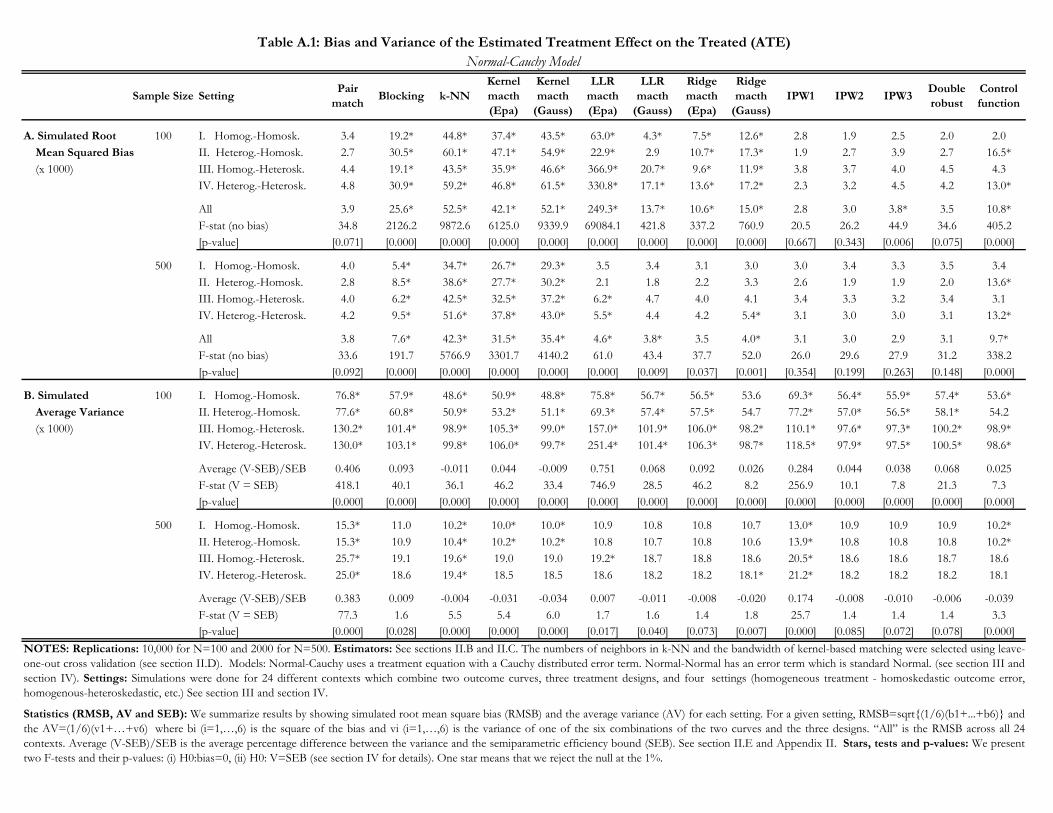
Sample Size SettingPair
matchBlocking k-NN
Kernel macth (Epa)
Kernel macth
(Gauss)
LLR macth (Epa)
LLR macth
(Gauss)
Ridge macth (Epa)
Ridge macth
(Gauss)IPW1 IPW2 IPW3
Double robust
Control function
A. Simulated Root 100 I. Homog.-Homosk. 3.4 19.2* 44.8* 37.4* 43.5* 63.0* 4.3* 7.5* 12.6* 2.8 1.9 2.5 2.0 2.0 Mean Squared Bias II. Heterog.-Homosk. 2.7 30.5* 60.1* 47.1* 54.9* 22.9* 2.9 10.7* 17.3* 1.9 2.7 3.9 2.7 16.5* (x 1000) III. Homog.-Heterosk. 4.4 19.1* 43.5* 35.9* 46.6* 366.9* 20.7* 9.6* 11.9* 3.8 3.7 4.0 4.5 4.3
IV. Heterog.-Heterosk. 4.8 30.9* 59.2* 46.8* 61.5* 330.8* 17.1* 13.6* 17.2* 2.3 3.2 4.5 4.2 13.0*
All 3.9 25.6* 52.5* 42.1* 52.1* 249.3* 13.7* 10.6* 15.0* 2.8 3.0 3.8* 3.5 10.8*F-stat (no bias) 34.8 2126.2 9872.6 6125.0 9339.9 69084.1 421.8 337.2 760.9 20.5 26.2 44.9 34.6 405.2[p-value] [0.071] [0.000] [0.000] [0.000] [0.000] [0.000] [0.000] [0.000] [0.000] [0.667] [0.343] [0.006] [0.075] [0.000]
500 I. Homog.-Homosk. 4.0 5.4* 34.7* 26.7* 29.3* 3.5 3.4 3.1 3.0 3.0 3.4 3.3 3.5 3.4II. Heterog.-Homosk. 2.8 8.5* 38.6* 27.7* 30.2* 2.1 1.8 2.2 3.3 2.6 1.9 1.9 2.0 13.6*III. Homog.-Heterosk. 4.0 6.2* 42.5* 32.5* 37.2* 6.2* 4.7 4.0 4.1 3.4 3.3 3.2 3.4 3.1IV. Heterog.-Heterosk. 4.2 9.5* 51.6* 37.8* 43.0* 5.5* 4.4 4.2 5.4* 3.1 3.0 3.0 3.1 13.2*
All 3.8 7.6* 42.3* 31.5* 35.4* 4.6* 3.8* 3.5 4.0* 3.1 3.0 2.9 3.1 9.7*F-stat (no bias) 33.6 191.7 5766.9 3301.7 4140.2 61.0 43.4 37.7 52.0 26.0 29.6 27.9 31.2 338.2[p-value] [0.092] [0.000] [0.000] [0.000] [0.000] [0.000] [0.009] [0.037] [0.001] [0.354] [0.199] [0.263] [0.148] [0.000]
B. Simulated 100 I. Homog.-Homosk. 76.8* 57.9* 48.6* 50.9* 48.8* 75.8* 56.7* 56.5* 53.6 69.3* 56.4* 55.9* 57.4* 53.6* Average Variance II. Heterog.-Homosk. 77.6* 60.8* 50.9* 53.2* 51.1* 69.3* 57.4* 57.5* 54.7 77.2* 57.0* 56.5* 58.1* 54.2 (x 1000) III. Homog.-Heterosk. 130.2* 101.4* 98.9* 105.3* 99.0* 157.0* 101.9* 106.0* 98.2* 110.1* 97.6* 97.3* 100.2* 98.9*
IV. Heterog.-Heterosk. 130.0* 103.1* 99.8* 106.0* 99.7* 251.4* 101.4* 106.3* 98.7* 118.5* 97.9* 97.5* 100.5* 98.6*
Average (V-SEB)/SEB 0.406 0.093 -0.011 0.044 -0.009 0.751 0.068 0.092 0.026 0.284 0.044 0.038 0.068 0.025F-stat (V = SEB) 418.1 40.1 36.1 46.2 33.4 746.9 28.5 46.2 8.2 256.9 10.1 7.8 21.3 7.3[p-value] [0.000] [0.000] [0.000] [0.000] [0.000] [0.000] [0.000] [0.000] [0.000] [0.000] [0.000] [0.000] [0.000] [0.000]
500 I. Homog.-Homosk. 15.3* 11.0 10.2* 10.0* 10.0* 10.9 10.8 10.8 10.7 13.0* 10.9 10.9 10.9 10.2*II. Heterog.-Homosk. 15.3* 10.9 10.4* 10.2* 10.2* 10.8 10.7 10.8 10.6 13.9* 10.8 10.8 10.8 10.2*III. Homog.-Heterosk. 25.7* 19.1 19.6* 19.0 19.0 19.2* 18.7 18.8 18.6 20.5* 18.6 18.6 18.7 18.6IV. Heterog.-Heterosk. 25.0* 18.6 19.4* 18.5 18.5 18.6 18.2 18.2 18.1* 21.2* 18.2 18.2 18.2 18.1
Average (V-SEB)/SEB 0.383 0.009 -0.004 -0.031 -0.034 0.007 -0.011 -0.008 -0.020 0.174 -0.008 -0.010 -0.006 -0.039F-stat (V = SEB) 77.3 1.6 5.5 5.4 6.0 1.7 1.6 1.4 1.8 25.7 1.4 1.4 1.4 3.3[p-value] [0.000] [0.028] [0.000] [0.000] [0.000] [0.017] [0.040] [0.073] [0.007] [0.000] [0.085] [0.072] [0.078] [0.000]
Table A.1: Bias and Variance of the Estimated Treatment Effect on the Treated (ATE)Normal-Cauchy Model
NOTES: Replications: 10,000 for N=100 and 2000 for N=500. Estimators: See sections II.B and II.C. The numbers of neighbors in k-NN and the bandwidth of kernel-based matching were selected using leave-one-out cross validation (see section II.D). Models: Normal-Cauchy uses a treatment equation with a Cauchy distributed error term. Normal-Normal has an error term which is standard Normal. (see section III andsection IV). Settings: Simulations were done for 24 different contexts which combine two outcome curves, three treatment designs, and four settings (homogeneous treatment - homoskedastic outcome error,homogenous-heteroskedastic, etc.) See section III and section IV.
Statistics (RMSB, AV and SEB): We summarize results by showing simulated root mean square bias (RMSB) and the average variance (AV) for each setting. For a given setting, RMSB=sqrt{(1/6)(b1+...+b6)} andthe AV=(1/6)(v1+…+v6) where bi (i=1,…,6) is the square of the bias and vi (i=1,…,6) is the variance of one of the six combinations of the two curves and the three designs. “All” is the RMSB across all 24contexts. Average (V-SEB)/SEB is the average percentage difference between the variance and the semiparametric efficiency bound (SEB). See section II.E and Appendix II. Stars, tests and p-values: We presenttwo F-tests and their p-values: (i) H0:bias=0, (ii) H0: V=SEB (see section IV for details). One star means that we reject the null at the 1%.

Misspec. TypeSettingPair
matchBlocking k-NN
Kernel macth (Epa)
Kernel macth
(Gauss)
LLR macth (Epa)
LLR macth
(Gauss)
Ridge macth (Epa)
Ridge macth
(Gauss)IPW1 IPW2 IPW3
Double robust
Control function
A. Simulated Root Xs I. Homog.-Homosk. 122.9* 120.0* 143.6* 141.8* 144.1* 111.5* 120.8* 126.0* 128.9* 121.6* 122.8* 123.2* 122.4* 124.5* Mean Squared Bias II. Heterog.-Homosk. 185.1* 182.1* 215.1* 211.3* 215.2* 180.0* 183.1* 189.6* 193.5* 183.0* 185.0* 185.5* 183.6* 186.6* (x 1000) III. Homog.-Heterosk. 123.6* 121.5* 142.9* 140.7* 145.1* 265.7* 117.2* 127.6* 129.4* 121.8* 123.5* 123.8* 123.2* 125.1*
IV. Heterog.-Heterosk. 184.2* 181.5* 211.8* 208.6* 214.5* 220.5* 177.7* 190.1* 192.1* 181.9* 184.0* 184.6* 183.3* 186.3*
All 157.0* 154.3* 181.8* 178.9* 183.1* 202.5* 152.8* 161.4* 164.1* 155.1* 156.8* 157.3* 156.1* 158.6*F-stat (no bias) 61775 78783 117000 112000 120000 78669 78860 85739 92318 76675 84121 84760 81267 85422[p-value] [0.000] [0.000] [0.000] [0.000] [0.000] [0.000] [0.000] [0.000] [0.000] [0.000] [0.000] [0.000] [0.000] [0.000]
Dist of u. I. Homog.-Homosk. 3.6 19.3* 45.3* 38.2* 44.3* 67.9* 5.3* 7.3* 12.6* 36.1* 2.5 2.3 2.1 1.9II. Heterog.-Homosk. 3.0 31.2* 61.2* 48.6* 56.2* 27.5* 4.5* 11.6* 17.3* 46.0* 4.4 4.6* 2.1 16.9*III. Homog.-Heterosk. 4.5 19.3* 43.7* 38.4* 48.1* 355.2* 25.7* 11.3* 12.3* 34.9* 6.1* 5.2 4.3 4.2IV. Heterog.-Heterosk. 5.1 31.6* 60.1* 50.5* 63.7* 321.2* 21.9* 16.7* 17.9* 47.0* 6.1* 6.8* 5.5 13.4*
All 4.1 26.1* 53.2* 44.3* 53.6* 242.2* 17.3* 12.2* 15.2* 41.4* 5.0* 5.0* 3.8 11.0*F-stat (no bias) 38.5 2187.6 10191.9 6682.6 9863.5 67751.5 653.5 426.4 777.2 2475.9 63.1 68.4 36.5 422.9[p-value] [0.031] [0.000] [0.000] [0.000] [0.000] [0.000] [0.000] [0.000] [0.000] [0.000] [0.000] [0.000] [0.049] [0.000]
B. Simulated Xs I. Homog.-Homosk. 66.5 49.6* 45.5* 45.7* 44.8* 57.4* 49.4* 49.2* 47.8* 52.9* 48.5* 48.4* 49.6* 48.1* Average Variance II. Heterog.-Homosk. 67.8 51.9* 47.0* 47.3* 46.3* 54.0* 50.8* 50.4* 48.9* 56.5* 49.4* 49.3* 50.6* 49.2* (x 1000) III. Homog.-Heterosk. 163.7* 123.9* 123.5* 128.8* 122.0* 184.3* 127.5* 130.8* 123.5* 125.8* 121.6* 121.5* 125.0* 125.5*
IV. Heterog.-Heterosk. 165.7* 126.5* 124.0* 129.5* 122.2* 269.5* 127.5* 131.6* 124.1* 129.4* 122.2* 122.1* 125.6* 125.8*
Average (V-SEB)/SEB 0.258 -0.046 -0.085 -0.059 -0.098 0.461 -0.040 -0.025 -0.070 -0.006 -0.074 -0.076 -0.050 -0.059F-stat (V = SEB) 299.5 352.3 602.7 614.4 647.6 804.9 391.2 422.2 462.3 228.9 418.0 423.2 372.3 445.4[p-value] [0.000] [0.000] [0.000] [0.000] [0.000] [0.000] [0.000] [0.000] [0.000] [0.000] [0.000] [0.000] [0.000] [0.000]
Dist of u. I. Homog.-Homosk. 76.8* 58.4* 48.4* 50.5* 48.6* 75.4* 57.1* 56.4* 53.8 93.0* 63.5* 58.7* 60.4* 53.4*II. Heterog.-Homosk. 77.4* 61.4* 50.5* 52.8* 50.9* 69.7* 57.9* 57.4* 54.8 111.2* 64.5* 59.3* 61.3* 54.1III. Homog.-Heterosk. 130.2* 102.0* 99.0* 105.2* 98.9* 153.7* 103.7* 106.1* 98.5* 153.4* 107.2* 101.0* 104.3* 98.8*IV. Heterog.-Heterosk. 130.0* 103.8* 99.7* 106.3* 99.8* 243.8* 102.7* 106.7* 98.9* 164.0* 107.7* 101.4* 104.8* 98.7*
Average (V-SEB)/SEB 0.405 0.102 -0.013 0.041 -0.011 0.722 0.081 0.093 0.028 0.767 0.161 0.083 0.118 0.024F-stat (V = SEB) 416.2 47.1 38.6 49.6 35.7 732.2 38.5 47.3 8.8 858.5 104.4 32.6 59.0 7.4[p-value] [0.000] [0.000] [0.000] [0.000] [0.000] [0.000] [0.000] [0.000] [0.000] [0.000] [0.000] [0.000] [0.000] [0.000]
Table A.2: Bias and Variance of the Estimated Treatment Effect on the Treated (ATE) under MisspecificationMisspecification of the Propensity Score in the Normal-Cauchy Model (sample size 100)
NOTES: Replications: 10,000 for N=100 and 2000 for N=500. Estimators: See sections II.B and II.C. The numbers of neighbors in k-NN and the bandwidth of kernel-based matching were selected using leave-one-out cross validation (see section II.D). Models: Normal-Cauchy uses a treatment equation with a Cauchy distributed error term. Normal-Normal has an error term which is standard Normal. (see section III andsection IV). Settings: Simulations were done for 24 different contexts which combine two outcome curves, three treatment designs, and four settings (homogeneous treatment - homoskedastic outcome error,homogenous-heteroskedastic, etc.) See section III and section IV.
Statistics (RMSB, AV and SEB): We summarize results by showing simulated root mean square bias (RMSB) and the average variance (AV) for each setting. For a given setting, RMSB=sqrt{(1/6)(b1+...+b6)} andthe AV=(1/6)(v1+…+v6) where bi (i=1,…,6) is the square of the bias and vi (i=1,…,6) is the variance of one of the six combinations of the two curves and the three designs. “All” is the RMSB across all 24contexts. Average (V-SEB)/SEB is the average percentage difference between the variance and the semiparametric efficiency bound (SEB). See section II.E and Appendix II. Stars, tests and p-values: We presenttwo F-tests and their p-values: (i) H0:bias=0, (ii) H0: V=SEB (see section IV for details). One star means that we reject the null at the 1%.
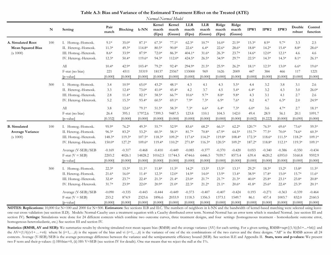
N SettingPair
matchBlocking k-NN
Kernel macth (Epa)
Kernel macth
(Gauss)
LLR macth (Epa)
LLR macth
(Gauss)
Ridge macth (Epa)
Ridge macth
(Gauss)IPW1 IPW2 IPW3
Double robust
Control function
A. Simulated Root 100 I. Homog.-Homosk. 9.1* 35.0* 87.1* 67.3* 77.1* 62.3* 10.7* 16.0* 21.9* 15.3* 8.9* 9.7* 3.3 2.5 Mean Squared Bias II. Heterog.-Homosk. 11.3* 49.3* 114.8* 80.5* 90.8* 22.6* 6.4* 22.6* 28.6* 18.8* 14.2* 15.4* 8.8* 28.6* (x 1000) III. Homog.-Heterosk. 8.6* 33.9* 87.9* 72.0* 86.3* 404.1* 31.6* 26.3* 23.7* 14.6* 12.0* 12.1* 4.6 4.6
IV. Heterog.-Heterosk. 12.3* 50.4* 119.6* 94.3* 112.0* 424.5* 26.5* 34.9* 29.7* 22.5* 14.3* 14.3* 8.1* 26.1*
All 10.4* 42.9* 103.4* 79.2* 92.4* 294.9* 21.5* 25.9* 26.2* 18.1* 12.5* 13.0* 6.6* 19.6*F-stat (no bias) 221 4511 35319 18137 25567 133000 969 1626 2009 447 384 466 117 1221[p-value] [0.000] [0.000] [0.000] [0.000] [0.000] [0.000] [0.000] [0.000] [0.000] [0.000] [0.000] [0.000] [0.000] [0.000]
500 I. Homog.-Homosk. 3.4 10.9* 65.0* 43.2* 48.1* 4.3 4.1 4.3 5.5* 4.4 3.2 3.8 3.1 2.6II. Heterog.-Homosk. 3.3 12.4* 73.0* 41.0* 45.4* 4.2 3.7 4.5 5.4* 6.4* 3.2 4.3 3.0 26.0*III. Homog.-Heterosk. 2.8 11.4* 82.1* 58.5* 66.7* 10.6* 9.7* 8.8* 9.8* 4.3 3.1 4.1 2.7 2.6IV. Heterog.-Heterosk. 5.2 15.3* 93.4* 60.5* 69.1* 7.9* 7.3* 6.9* 7.6* 8.2 4.7 6.3* 2.0 24.9*
All 3.8 12.6* 79.1* 51.5* 58.3* 7.3* 6.6* 6.4* 7.3* 6.0* 3.6 4.7* 2.7 18.1*F-stat (no bias) 26.4 395.1 17972.6 7399.3 9487.5 123.8 110.1 104.3 142.0 49.4 28.9 56.1 20.1 1091.7[p-value] [0.332] [0.000] [0.000] [0.000] [0.000] [0.000] [0.000] [0.000] [0.000] [0.002] [0.222] [0.000] [0.690] [0.000]
B. Simulated 100 I. Homog.-Homosk. 95.9* 76.2* 49.3* 55.7* 52.9* 83.6* 68.2* 66.1* 62.2* 120.7* 76.5* 69.6* 73.6* 59.5* Average Variance II. Heterog.-Homosk. 96.3* 83.2* 53.2* 60.3* 58.1* 81.7* 70.8* 67.9* 64.5* 151.7* 77.5* 70.0* 74.6* 60.3* (x 1000) III. Homog.-Heterosk. 148.3* 119.3* 107.5* 118.3* 109.2* 117.6* 114.2* 119.8* 108.4* 172.3* 118.6* 111.5* 118.2* 109.1*
IV. Heterog.-Heterosk. 150.0* 127.2* 109.6* 119.4* 110.2* 271.8* 116.3* 120.5* 109.2* 187.2* 118.8* 112.1* 119.3* 109.1*
Average (V-SEB)/SEB -0.169 -0.317 -0.468 -0.410 -0.449 -0.085 -0.377 -0.370 -0.420 0.053 -0.340 -0.386 -0.350 -0.434F-stat (V = SEB) 2203.2 4026.1 14828.2 10162.5 11744.5 4744.6 6446.5 7039.7 8573.4 639.4 4620.2 6593.0 5160.8 9592.9[p-value] [0.000] [0.000] [0.000] [0.000] [0.000] [0.000] [0.000] [0.000] [0.000] [0.000] [0.000] [0.000] [0.000] [0.000]
500 I. Homog.-Homosk. 22.3* 15.3* 11.1* 11.8* 11.5* 14.2* 13.5* 13.5* 13.1* 29.2* 18.3* 15.2* 15.8* 11.5*II. Heterog.-Homosk. 21.6* 16.0* 11.4* 12.3* 12.0* 14.9* 14.0* 13.9* 13.4* 38.9* 17.8* 15.0* 15.7* 11.6*III. Homog.-Heterosk. 32.4* 23.7* 22.4* 21.3* 21.4* 23.0* 21.7* 21.7* 21.3* 40.0* 25.8* 23.1* 23.8* 20.8*IV. Heterog.-Heterosk. 31.7* 23.9* 22.0* 20.9* 21.0* 22.3* 21.2* 21.1* 20.6* 41.8* 25.6* 22.4* 23.3* 20.1*
Average (V-SEB)/SEB -0.090 -0.335 -0.443 -0.444 -0.449 -0.373 -0.407 -0.407 -0.424 0.193 -0.271 -0.363 -0.339 -0.464F-stat (V = SEB) 253.2 874.9 2323.6 1896.6 2033.9 1118.3 1356.5 1373.1 1549.7 86.1 457.4 1003.7 832.0 2160.5[p-value] [0.000] [0.000] [0.000] [0.000] [0.000] [0.000] [0.000] [0.000] [0.000] [0.000] [0.000] [0.000] [0.000] [0.000]
Statistics (RMSB, AV and SEB): We summarize results by showing simulated root mean square bias (RMSB) and the average variance (AV) for each setting. For a given setting, RMSB=sqrt{(1/6)(b1+...+b6)} andthe AV=(1/6)(v1+…+v6) where bi (i=1,…,6) is the square of the bias and vi (i=1,…,6) is the variance of one of the six combinations of the two curves and the three designs. “All” is the RMSB across all 24contexts. Average (V-SEB)/SEB is the average percentage difference between the variance and the semiparametric efficiency bound (SEB). See section II.E and Appendix II. Stars, tests and p-values: We presenttwo F-tests and their p-values: (i) H0:bias=0, (ii) H0: V=SEB (see section IV for details). One star means that we reject the null at the 1%.
NOTES: Replications: 10,000 for N=100 and 2000 for N=500. Estimators: See sections II.B and II.C. The numbers of neighbors in k-NN and the bandwidth of kernel-based matching were selected using leave-one-out cross validation (see section II.D). Models: Normal-Cauchy uses a treatment equation with a Cauchy distributed error term. Normal-Normal has an error term which is standard Normal. (see section III andsection IV). Settings: Simulations were done for 24 different contexts which combine two outcome curves, three treatment designs, and four settings (homogeneous treatment - homoskedastic outcome error,homogenous-heteroskedastic, etc.) See section III and section IV.
Table A.3: Bias and Variance of the Estimated Treatment Effect on the Treated (ATE)Normal-Normal Model

Trimming SettingPair
matchBlocking k-NN
Kernel macth (Epa)
Kernel macth
(Gauss)
LLR macth (Epa)
LLR macth
(Gauss)
Ridge macth (Epa)
Ridge macth
(Gauss)IPW1 IPW2 IPW3
Double robust
Control function
Rule 1 I. Homog.-Homosk. 5.7* 28.1* 51.7* 43.5* 49.7* 75.3* 6.1* 12.7* 16.5* 71.2* 4.4 3.8 3.3 2.9II. Heterog.-Homosk. 23.5* 30.6* 64.1* 49.4* 56.1* 37.0* 19.8* 24.2* 25.2* 111.1* 24.5* 22.2* 27.2* 35.5*III. Homog.-Heterosk. 3.8 29.3* 47.9* 39.0* 49.2* 374.2* 22.6* 13.7* 13.8* 69.8* 8.5* 5.7 5.0 4.8IV. Heterog.-Heterosk. 18.4* 32.6* 62.4* 49.0* 61.8* 379.8* 13.4* 22.1* 20.1* 109.4* 19.4* 16.6* 21.9* 30.2*
All 15.3* 30.2* 57.0* 45.4* 54.5* 269.9* 16.7* 18.9* 19.4* 92.6* 16.3* 14.3* 17.7* 23.5*F-stat (no bias) 508.0 2230.7 9461.0 5589.7 8332.2 97336.0 686.3 922.0 1100.6 12451.3 711.3 575.3 863.1 1594.7[p-value] [0.000] [0.000] [0.000] [0.000] [0.000] [0.000] [0.000] [0.000] [0.000] [0.000] [0.000] [0.000] [0.000] [0.000]
Rule 2 I. Homog.-Homosk. 18.9* 112.5* 97.6* 78.2* 86.6* 61.0* 15.7* 23.9* 29.3* 85.8* 55.9* 41.8* 2.9 2.6II. Heterog.-Homosk. 21.6* 173.4* 126.3* 92.5* 101.2* 26.1* 12.4* 29.2* 35.2* 134.7* 78.8* 57.2* 20.9* 31.4*III. Homog.-Heterosk. 15.2* 113.7* 95.8* 80.7* 93.9* 399.0* 37.4* 32.4* 28.5* 85.5* 52.9* 38.8* 4.3 4.3IV. Heterog.-Heterosk. 24.6* 175.8* 132.3* 108.4* 124.7* 416.0* 35.1* 45.0* 39.2* 136.5* 80.2* 58.6* 17.9* 26.3*
All 20.4* 147.1* 114.2* 90.8* 102.6* 290.1* 27.5* 33.5* 33.3* 113.4* 68.1* 49.9* 14.0* 20.6*F-stat (no bias) 689.5 47809.4 41096.3 22584.5 29204.9 124000 1469.6 2550.6 2945.1 32887.1 14341.6 7340.5 517.5 1253.8[p-value] [0.000] [0.000] [0.000] [0.000] [0.000] [0.000] [0.000] [0.000] [0.000] [0.000] [0.000] [0.000] [0.000] [0.000]
Rule 3 I. Homog.-Homosk. 5.2* 23.4* 47.1* 39.9* 45.5* 85.6* 6.7* 11.8* 15.4* 17.8* 5.9* 2.7 3.7 3.2II. Heterog.-Homosk. 24.5* 23.0* 59.4* 46.9* 53.3* 46.4* 20.4* 26.1* 26.8* 46.1* 29.2* 26.0* 25.1* 34.0*III. Homog.-Heterosk. 4.9 25.4* 44.1* 36.0* 46.0* 382.4* 25.5* 12.6* 12.8* 16.3* 11.1* 7.1* 6.2* 5.5IV. Heterog.-Heterosk. 18.0* 25.6* 57.2* 44.9* 56.9* 397.4* 16.1* 21.6* 20.0* 40.5* 23.6* 19.9* 18.6* 27.5*
All 15.6* 24.4* 52.3* 42.1* 50.7* 280.0* 18.5* 19.0* 19.5* 33.0* 19.8* 16.8* 16.0* 22.1*F-stat (no bias) 514.0 1395.2 7450.2 4479.7 6758.0 105000 765.5 896.2 1061.9 1810.1 995.5 755.6 680.0 1341.8[p-value] [0.000] [0.000] [0.000] [0.000] [0.000] [0.000] [0.000] [0.000] [0.000] [0.000] [0.000] [0.000] [0.000] [0.000]
Rule 4 I. Homog.-Homosk. 5.1* 36.3* 57.3* 47.7* 54.4* 62.2* 6.3* 12.8* 16.4* 4.0 2.5 3.8 2.6 2.6II. Heterog.-Homosk. 25.2* 43.3* 72.4* 56.4* 64.1* 24.4* 21.7* 27.1* 28.6* 29.6* 25.4* 24.9* 26.7* 34.8*III. Homog.-Heterosk. 3.5 37.7* 53.8* 43.7* 55.3* 381.7* 22.7* 15.3* 13.7* 6.0 4.7 4.0 5.1 4.8IV. Heterog.-Heterosk. 20.0* 46.0* 71.8* 55.7* 71.3* 388.9* 15.6* 26.4* 23.4* 24.6* 20.1* 19.5* 21.5* 29.7*
All 16.4* 41.0* 64.4* 51.2* 61.7* 274.5* 17.8* 21.4* 21.4* 19.6* 16.4* 16.1* 17.4* 23.0*F-stat (no bias) 613.6 4394.9 12593.3 7379.7 11116.8 115000 835.3 1207.1 1394.1 891.8 802.5 781.6 877.8 1599.7[p-value] [0.000] [0.000] [0.000] [0.000] [0.000] [0.000] [0.000] [0.000] [0.000] [0.000] [0.000] [0.000] [0.000] [0.000]
NOTES: Replications: 10,000 for N=100 and 2000 for N=500. Estimators: See sections II.B and II.C. The numbers of neighbors in k-NN and the bandwidth of kernel-based matching were selected using leave-one-out cross validation (see section II.D). Models: Normal-Cauchy uses a treatment equation with a Cauchy distributed error term. Normal-Normal has an error term which is standard Normal. (see section III andsection IV). Settings: Simulations were done for 24 different contexts which combine two outcome curves, three treatment designs, and four settings (homogeneous treatment - homoskedastic outcome error,homogenous-heteroskedastic, etc.) See section III and section IV.Statistics (RMSB, AV and SEB): We summarize results by showing simulated root mean square bias (RMSB) and the average variance (AV) for each setting. For a given setting, RMSB=sqrt{(1/6)(b1+...+b6)} andthe AV=(1/6)(v1+…+v6) where bi (i=1,…,6) is the square of the bias and vi (i=1,…,6) is the variance of one of the six combinations of the two curves and the three designs. “All” is the RMSB across all 24contexts. Average (V-SEB)/SEB is the average percentage difference between the variance and the semiparametric efficiency bound (SEB). See section II.E and Appendix II. Stars, tests and p-values: We presenttwo F-tests and their p-values: (i) H0:bias=0, (ii) H0: V=SEB (see section IV for details). One star means that we reject the null at the 1%.
Table A.4: Simulated Root Mean Squared Bias (x 1000) of the Estimated Treatment Effect on the Treated (ATE)Trimming Results in the Normal-Normal Model (Sample size 100)
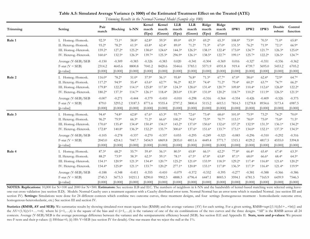
Trimming SettingPair
matchBlocking k-NN
Kernel macth (Epa)
Kernel macth
(Gauss)
LLR macth (Epa)
LLR macth
(Gauss)
Ridge macth (Epa)
Ridge macth
(Gauss)IPW1 IPW2 IPW3
Double robust
Control function
Rule 1 I. Homog.-Homosk. 92.3* 73.1* 58.8* 62.8* 59.5* 89.0* 69.3* 69.2* 65.3* 108.8* 73.9* 70.5* 71.0* 65.8*II. Heterog.-Homosk. 93.2* 78.2* 61.5* 65.8* 62.4* 89.0* 71.2* 71.3* 67.0* 131.5* 76.2* 71.9* 72.1* 66.9*III. Homog.-Heterosk. 159.2* 127.2* 125.2* 138.6* 124.6* 144.3* 126.5* 138.1* 122.4* 173.0* 124.7* 121.7* 126.3* 125.0*IV. Heterog.-Heterosk. 160.6* 132.5* 126.3* 139.7* 125.3* 296.9* 126.1* 138.5* 122.7* 199.1* 125.7* 122.2* 126.5* 124.7*
Average (V-SEB)/SEB -0.150 -0.309 -0.383 -0.326 -0.383 0.020 -0.341 -0.304 -0.369 0.016 -0.327 -0.351 -0.336 -0.362F-stat (V = SEB) 2314.2 4645.6 8800.8 7041.2 8420.6 3544.6 5783.1 5571.9 6931.8 919.4 4739.7 5695.0 5453.2 6705.2[p-value] [0.000] [0.000] [0.000] [0.000] [0.000] [0.000] [0.000] [0.000] [0.000] [0.000] [0.000] [0.000] [0.000] [0.000]
Rule 2 I. Homog.-Homosk. 116.0* 78.2* 51.0* 57.9* 56.1* 95.8* 76.8* 71.3* 67.7* 67.0* 58.6* 62.4* 72.9* 64.7*II. Heterog.-Homosk. 117.2* 94.9* 55.4* 63.6* 62.7* 96.2* 82.3* 74.4* 71.2* 79.4* 60.2* 63.7* 74.7* 66.2*III. Homog.-Heterosk. 179.8* 122.2* 114.1* 125.8* 117.8* 124.3* 128.6* 131.4* 120.7* 109.8* 110.4* 112.6* 126.8* 122.2*IV. Heterog.-Heterosk. 180.2* 137.3* 114.7* 126.1* 118.4* 283.0* 131.8* 131.0* 120.2* 118.7* 110.2* 111.9* 126.5* 121.5*
Average (V-SEB)/SEB -0.007 -0.271 -0.444 -0.379 -0.410 -0.010 -0.298 -0.316 -0.364 -0.354 -0.426 -0.409 -0.326 -0.375F-stat (V = SEB) 879.0 3293.2 13187.5 8771.6 9335.4 2797.2 3800.4 5115.2 6013.1 7814.3 11278.8 8934.6 5173.4 6987.5[p-value] [0.000] [0.000] [0.000] [0.000] [0.000] [0.000] [0.000] [0.000] [0.000] [0.000] [0.000] [0.000] [0.000] [0.000]
Rule 3 I. Homog.-Homosk. 94.4* 74.8* 62.8* 67.6* 63.3* 93.7* 72.6* 73.4* 68.6* 101.0* 75.9* 73.2* 74.2* 70.0*II. Heterog.-Homosk. 96.2* 79.9* 66.3* 71.2* 66.6* 100.2* 74.6* 75.9* 70.7* 115.1* 78.0* 75.0* 75.8* 71.5*III. Homog.-Heterosk. 170.6* 135.4* 134.4* 150.4* 134.1* 143.2* 137.0* 150.6* 132.6* 157.2* 132.9* 131.3* 136.1* 134.2*IV. Heterog.-Heterosk. 172.8* 140.8* 136.3* 152.2* 135.7* 300.6* 137.6* 151.6* 133.7* 173.1* 134.0* 132.1* 137.3* 134.5*
Average (V-SEB)/SEB -0.105 -0.278 -0.337 -0.270 -0.337 0.055 -0.295 -0.249 -0.323 -0.083 -0.296 -0.310 -0.292 -0.316F-stat (V = SEB) 2043.0 4214.1 7047.7 5454.9 6869.8 2835.0 4811.6 4449.4 5771.7 1315.1 4129.2 4817.5 4555.0 5394.8[p-value] [0.000] [0.000] [0.000] [0.000] [0.000] [0.000] [0.000] [0.000] [0.000] [0.000] [0.000] [0.000] [0.000] [0.000]
Rule 4 I. Homog.-Homosk. 87.3* 68.2* 55.7* 59.4* 56.1* 80.5* 65.8* 66.1* 62.2* 77.8* 66.4* 65.4* 67.4* 63.3*II. Heterog.-Homosk. 88.2* 73.9* 58.3* 62.3* 59.1* 78.1* 67.5* 67.8* 63.8* 87.1* 68.0* 66.6* 68.4* 64.5*III. Homog.-Heterosk. 154.1* 120.9* 121.3* 134.4* 120.7* 125.2* 121.0* 133.9* 118.5* 129.2* 117.4* 116.8* 121.6* 120.2*IV. Heterog.-Heterosk. 154.4* 125.8* 121.1* 133.7* 120.2* 277.1* 120.8* 133.1* 117.8* 136.3* 117.3* 116.4* 121.4* 119.9*
Average (V-SEB)/SEB -0.188 -0.348 -0.411 -0.355 -0.410 -0.079 -0.372 -0.332 -0.395 -0.277 -0.381 -0.388 -0.366 -0.386F-stat (V = SEB) 2745.3 5673.3 10211.1 8290.0 9902.3 4888.3 6796.4 6447.1 8003.3 3594.1 6781.5 7165.9 6439.9 7546.3[p-value] [0.000] [0.000] [0.000] [0.000] [0.000] [0.000] [0.000] [0.000] [0.000] [0.000] [0.000] [0.000] [0.000] [0.000]
Statistics (RMSB, AV and SEB): We summarize results by showing simulated root mean square bias (RMSB) and the average variance (AV) for each setting. For a given setting, RMSB=sqrt{(1/6)(b1+...+b6)} andthe AV=(1/6)(v1+…+v6) where bi (i=1,…,6) is the square of the bias and vi (i=1,…,6) is the variance of one of the six combinations of the two curves and the three designs. “All” is the RMSB across all 24contexts. Average (V-SEB)/SEB is the average percentage difference between the variance and the semiparametric efficiency bound (SEB). See section II.E and Appendix II. Stars, tests and p-values: We presenttwo F-tests and their p-values: (i) H0:bias=0, (ii) H0: V=SEB (see section IV for details). One star means that we reject the null at the 1%.
NOTES: Replications: 10,000 for N=100 and 2000 for N=500. Estimators: See sections II.B and II.C. The numbers of neighbors in k-NN and the bandwidth of kernel-based matching were selected using leave-one-out cross validation (see section II.D). Models: Normal-Cauchy uses a treatment equation with a Cauchy distributed error term. Normal-Normal has an error term which is standard Normal. (see section III andsection IV). Settings: Simulations were done for 24 different contexts which combine two outcome curves, three treatment designs, and four settings (homogeneous treatment - homoskedastic outcome error,homogenous-heteroskedastic, etc.) See section III and section IV.
Trimming Results in the Normal-Normal Model (Sample size 100)Table A.5: Simulated Average Variance (x 1000) of the Estimated Treatment Effect on the Treated (ATE)

Setting Design Curve CRLB SEB CRLB SEB CRLB SEB CRLB SEB CRLB SEB CRLB SEB
I A 1 4.70 4.79 5.32 5.58 4.49 6.37 4.65 8.73 5.81 24.07 7.56 44.14A 2 4.51 4.79 5.39 5.58 4.28 6.37 4.51 8.73 5.61 24.07 9.60 44.14B 1 5.47 5.70 6.29 6.80 4.54 6.98 4.68 9.45 5.71 9.85 7.44 17.63B 2 5.56 5.70 6.75 6.80 4.27 6.98 4.43 9.45 6.34 9.85 9.82 17.63C 1 5.37 5.70 6.05 6.39 4.41 6.98 4.57 9.34 5.60 9.85 6.78 10.02C 2 4.80 5.70 5.24 6.39 4.19 6.98 4.37 9.34 4.79 9.85 6.21 10.02
II A 1 4.66 4.81 5.39 5.61 4.58 6.40 4.77 8.79 6.00 24.11 7.93 44.20A 2 4.55 4.80 5.44 5.59 4.24 6.38 4.50 8.76 5.68 24.09 9.65 44.19B 1 5.50 5.71 6.34 6.82 4.47 7.01 4.71 9.48 5.69 9.88 7.24 17.66B 2 5.55 5.70 6.74 6.81 4.44 6.99 4.68 9.47 6.37 9.87 9.82 17.66C 1 5.46 5.71 6.14 6.45 4.39 7.01 4.64 9.44 5.77 9.88 6.88 10.08C 2 4.64 5.70 4.99 6.40 4.35 6.99 4.60 9.38 4.57 9.86 5.87 10.05
III A 1 8.48 8.79 9.49 10.14 8.85 10.37 11.81 13.91 9.42 28.07 11.08 49.40A 2 8.70 8.79 9.75 10.14 8.30 10.37 10.41 13.91 10.26 28.07 13.30 49.40B 1 8.79 9.70 9.75 11.13 8.75 10.98 11.67 14.17 8.72 13.85 10.19 22.32B 2 9.22 9.70 10.30 11.13 8.31 10.98 10.37 14.17 9.87 13.85 12.12 22.32C 1 9.50 9.70 11.02 11.62 8.57 10.98 11.48 15.27 9.91 13.85 11.60 15.49C 2 9.17 9.70 10.02 11.62 8.23 10.98 10.33 15.27 9.62 13.85 11.34 15.49
IV A 1 8.42 8.81 9.44 10.17 8.90 10.40 12.01 13.96 9.46 28.11 11.37 49.46A 2 8.51 8.80 9.43 10.15 8.42 10.38 10.67 13.94 10.07 28.09 12.93 49.45B 1 8.77 9.71 9.72 11.14 8.90 11.01 12.07 14.20 8.90 13.88 10.39 22.36B 2 9.50 9.70 10.56 11.14 8.49 10.99 10.77 14.19 10.01 13.87 12.33 22.36C 1 9.51 9.71 11.22 11.67 8.82 11.01 11.88 15.37 9.88 13.88 11.72 15.55C 2 9.32 9.70 10.26 11.62 8.25 10.99 10.43 15.31 9.87 13.86 11.68 15.52
NOTES: See section II.E and Appendix II for details on the computation of the SEB. The CRLB was computed assuming full knowledge of the parametric model.
Table A.6. Cramer-Rao and Semiparametric Efficiency Bounds
ATE TOT
Cauchy
ATE TOT
Cauchy Misspecified Normal
ATE TOT
59