Finite range scattering wave function method for ...

Finite range scattering wave function method for scattering and resonance lifetimes

Hyo Weon Jang and John C. Light Department of Chemistry and The James Franck Institute, The University of Chicago, Chicago, Illinois 6063 7

(Received 25 January 1993; accepted 2 April 1993)

A generic expression for the scattering wave function in terms of the full discrete spectral Green’s function on a finite range is used to obtain the “finite range scattering wave function (FRSW)” which is accurate over a finite range of the scattering coordinate. We show that the representation of the FRSW in a finite basis set can be used to compute the scattering matrix and related quantities when the interaction potential is also restricted to this range. Comparisons of numerical results for several model problems with those of other methods and with analytical results indicate that the FRSW method is very accurate when converged and requires comparable or less computation than other methods. The main difference between the present method and other variational scattering methods is that the real Green’s function is used and that the scattering wave function itself is calculated nonvariationally. Thus the FRSW can be used to solve quantum mechanical problems involving scattering wave functions over a finite range such as scattering theory, resonance studies, and photodissociation. Results of two implementations are presented. Both require only one representation of the real Green’s function in a finite basis. One requires energy dependent matrix elements, while the other does not.

I. INTRODUCTION

Some years ago, several quantum scattering numerical methods were developed involving the full Green’s operator directly or indirectly.1V2 Although the details of the formulations differ, they are all variational methods using L2 bases. They are obtained by extremizing a particular functional of the trial wave function such as the S matrix. Also there are other methods which involve the Lippmann-Schwinger equation and treat it variationally or nonvariationally.3 Numerical applications of these methods to model problems and to three-dimensional reactive scattering problems have shown their efficiency, accuracy, and stability.‘-3

In this paper, we present another method which can be applied, in principle, to any quantum mechanical problem formulated in terms of scattering wave functions such as scattering theory, resonance studies, and photodissociation. In contrast to other methods which explicitly evaluate the wave functions over all space, we focus on evaluation of the wave functions in a finite range, but one which is sufficiently large to determine the asymptotic behaviors, i.e., the S matrix. While the scattering wave function cannot be expanded properly by a finite number of square integrable functions on an infinite range, it is possible to do so for a finite range. This may be fruitful if the interaction potential also acts only over the finite range. A generic expression for the exact scattering wave function on a finite range is developed in terms of the exact real L2 Green’s function on this range and one additional function, which may be an exact eigenfunction of the asymptotic Hamiltonian, or, in fact, an energy-independent arbitrary function. The resulting expression is named “finite range scattering wave function (FRSW).” The accurate scattering wave function may then be represented by a finite basis in this finite range.

This generic expression has been less utilized than the analogous Lippmann-Schwinger equation4 probably because of the expected difficulty in representing the full Green’s operator by a finite basis set. We show, however, that a finite basis set can be used to represent the FRSW, replacing the complete basis set for practical purposes, and the resulting approximation of the FRSW is shown to be useful for scattering calculations in regard to accuracy, efficiency, and simplicity. This method is used to calculate the S matrix and the energy derivative of S matrix in this paper, which are the essence of the cross section calculations and resonance lifetime studies.5

In the FRSW method, the calculated S matrix satisfies only SS*=S*S=I (it is not unitary or symmetric automatically, although it becomes so numerically as the basis size and the range are increased). However, this method is easily adapted to calculate the K matrix (reactance matrix)3’4 which, when symmetrized, yields a unitary and symmetric S matrix. Other characteristics of the FRSW method are that ( 1) it is a direct, but nonvariational approach to the scattering wave function; (2) no arbitrary cut-off functions or optical potentials are used; (3) real quantities only are used until the final evaluation of the S matrix; (4) only a single diagonalization of the real Green’s function is used over a wide range of energy; (5) either local surface or global volume projections onto energy dependent asymptotic wave functions may be used with comparable accuracy; and (6) energy derivatives of the S matrix can be determined which permits evaluation of resonance time delays or lifetimes.

The nonunitarity of the calculated S matrix indicates that the range is not extended to the asymptotic region and/or that the size of the basis set is not large enough to accommodate the dynamics for the chosen range. There- fore the extent of nonunitarity is useful as a barometer

J. Chem. Phys. 99 (2), 15 July 1993 0021-9606/93/99(2)/l 057/l 3/$6.00 @ 1993 American Institute of Physics 1057 Downloaded 16 Aug 2003 to 128.135.132.83. Redistribution subject to AIP license or copyright, see http://ojps.aip.org/jcpo/jcpcr.jsp

1058 H. W. Jang and J. C. Light: Finite range scattering wave function method

checking the adequacy of the calculated S matrix. At the same time, a more physically acceptable S matrix can be obtained either through a symmetric orthogonalization6 of the calculated S matrix to a symmetric and unitary form or by calculating the K matrix, symmetrizing, and then calculating the S matrix.

asymptotic Hamiltonian Ho. We later will show that an energy independent auxiliary function F can be used instead, with substantial increase in efficiency and little, if any, loss in accuracy. The derivation for @ is first. Let \I’ be the desired solution to the Schrbdinger equation of the full Hamiltonian H for a given initial state j,

The characteristics of the FRSW make it a suitable tool to solve quantum mechanical problems such as photodissociation in addition to scattering theory and resonance studies, mainly because the FRSW is a direct evaluation of the scattering wave functions, not an operator or a matrix element. Only one real matrix diagonalization is required to study resonance states in the present method, while a series of matrix diagonalizations (real or complex) must be done in the alternative approaches such as the stabilization method, complex rotation/scaling method, and the optical potential method.7-9 We present two ways of defming the FRSW. In one, the integrals appearing in the defining equation of the FRSW are energy dependent, while in the other, they are energy independent. The latter makes the FRSW method much more efficient for multiple energy calculations as are required, e.g., for highly accurate resonance state studies.

(E-H)Yj=O, (2.la)

and ~j be a certain linear combination of all independent regular solutions #i for the asymptotic Hamiltonian H,, with normalization to be determined later

(E-Ho)@i=O, ~j= C Cij(E)$i(E) i

(2.lb)

(for convenience, we drop the initial state label j below except where needed). We note that @ does not satisfy specified scattering boundary conditions for translation and therefore the real solutions may be used. Then, sub- traction of

The derivations of the FRSW and the theoretical as- pects of its application to scattering theory and resonance studies are given in Sec. II, which is followed by numerical applications to simple model problems of scattering and resonances in Sec. III. Finally, Sec. IV contains the con- clusions of this paper.

(E-H)@= (H,,-H)@= - V@

from Eq. (2. la) gives

(2.lc)

(E-H)(Y-@)=VQ, (2.ld)

II. THEORY

In this section, we present the basic theory of the finite range scattering wave function and the specifics of its implementation. In the first section below, we derive the basic equations for two types of auxiliary functions Cp, which is a real regular solution of an asymptotic Hamiltonian at energy E; and F, which is an energy independent regular function at the origin, is linearly independent of the L2 basis, and has a boundary condition different from that of the L2 basis at the end of the range. We then give the expressions if a discrete variable representation of the L2 basis is used. In Sec. II C, we give the expressions for the S matrix in terms of the FRSW evaluated at two points near the boundary of the L2 basis and discuss the measures of unitarity and the use of a symmetrized K matrix to evaluate the S matrix. In addition, we define the lifetime matrix Q used for resonances. Finally, in Sec. II D, we show how the range may be partitioned so that two or more smaller L2 bases may be used, and the FRSW constructed by forc- ing continuity on an overlapping region.

where V is the interaction potential equal to H-H,. After operating with (E-H) - ’ on Eq. (2. Id), one gets a generic expression of the scattering wave function

Y-@=(E-H)-‘VQ+CY, (2.le)

where C is an arbitrary constant and we indicate explicitly that the normalization must be determined. Remembering that @ has arbitrary normalization to be determined, we may write the exact solution as

Y=(E-H)-‘V@+@, (2.lf)

A. Derivation of FRSW

In this section, we present expressions for the scattering wave function defined on a finite range of the scattering coordinate using the full Green’s operator4 (E--H) - ‘. We assume that there are internal degrees of freedom in addition to the translational scattering coordinate.

We first give the derivation using an auxiliary function @ made up of regular eigenfunctions at energy E of an

i.e., the desired \I, can be expressed by Eq. (2.lf), where @ is a certain linear combination of all independent regular solutions pi for Ho with the expansion coefficients (normalization) to be determined. On the face of it, Eq. (2.lf) looks implausible since we have not imposed scattering boundary conditions. However, @ in Eq. (2. If), in contrast to the Lippmann-Schwinger equation, is a linear combination of pi determined for each initial state j by choosing the set of complex constants Cij( E) in Eq. (2. lb) which yield the correct flux normalized Yj(E). We now consider the evaluation of Eq. (2. lf) on a finite coordinate range which extends into the region in which V-+0, but not r-+c4.

A complete real orthonormal basis set { 1 m)} is defined on a finite range (r, ,rz), satisfying some boundary condition at r2, and the same boundary condition at the origin (rl) as Y and a. We assume that 1 m)‘s are eigen-

J. Chem. Phys., Vol. 99, No. 2, 15 July 1993

Downloaded 16 Aug 2003 to 128.135.132.83. Redistribution subject to AIP license or copyright, see http://ojps.aip.org/jcpo/jcpcr.jsp

functions of H. The completeness relation composed of { Im)} applied to Eq. (2.lf) gives the finite range scattering wave function (FRSW)

Y= 5 Im)(mI(E-H)-lVI<P)+@ m

= z Im)(E-E~)-l(ml VI@)+@. (2. w

Equation (2.lg) represents the set of exact solutions Y,(E) on the finite range.

The appropriate expansion coefficients for & in @ and the basis boundary conditions must now be found to determine the desired Y. Since Y is required to be regular at the origin and bounded over the whole space in a scattering problem, the basis set should be chosen to be regular and $i to be the bounded and regular solutions for Ho in Eq. (2.lg). At this stage, the remaining arbitrariness in the right hand side of Eq. (2. lg) can be eliminated by evaluating it in the “near asymptotic region” around r2. This depends on the outer boundary condition on the basis and on the expansion coefficients for oi in <p. This freedom to choose the expansion coefficients is necessary for Y to have the proper functional form in the asymptotic region of r<r2. Since the boundary condition of Y at r2 is not known a priori, it is determined by choosing the expansion coefficients for 4i such that Y has the correct asymptotic functional form near r,. This is possible as long as pi and Y are linearly independent of the basis, e.g., both do not satisfy zero boundary condition of the basis at r2 (see Sec. III).

An extremely important simplification is also possible using a different auxiliary function. We can choose a simple energy independent set of regular functions &, which are not eigenfunctions of H,, instead of & for Eqs. (2.la)- (2. lg) with minimal modifications of the formulas. In particular, substituting the negative of the left-hand side of Eq. (2.1~) rather than the right-hand side in Eq. (2.lf), we have another expression for Y,

Y=(E-H)-‘[(H-E)F]+F. (2.2)

Now F must be a linear combination of &, each of which is an internal state basis function times a regular energy independent translational function [fi( r) or a single f(r)]. This translational function(s) must be linearly independent of the L2 translational basis used for the representation of (E-H) - ’ and satisfy different boundary conditions at the outer boundary. As long as F in our implementation does not lie entirely in the space spanned by our representations of (E-H) -‘, then Eq. (2.2) is a valid expression. Results of both approaches will be presented later.

It is clear from the assumptions made thus far that the FRSW is not determined at the energies of the singularities of the Green’s function E=E,,,. The singularity of the Green’s function turns out not to be a problem, since the S matrix determined from Y remains finite at E= E,,, to com- puter accuracy. The auxiliary function Q (or F) must, however, be linearly independent (different boundary conditions) of the basis used to represent (E-H)-‘. For a

fixed range, this may be a problem with the energy dependent method as 4 ,(E) may go to zero at r,, for example. It is, however, easily removed by changing r2 or avoiding the troublesome E. Certainly there are no such troublesome energies in the “energy-independent-integral” scheme [Eq. (2.2)]. Finally, in the implementations below, r2 should lie in the asymptotic ( VrO) region for accurate results.

B. A finite basis for the FRSW utilizing the DVR

To obtain a practical tool for solving quantum mechanical problems, we develop an approximate expression for the FRSW in this section, replacing the complete basis set with a finite basis set, in particular, a discrete variable representation (DVR) basis set.” Unless otherwise specified, the translational basis spans a finite range and satisfies zero boundary conditions at both ends. For simplicity, we present the energy-dependent scheme first.

A projection operator is defined P= 8: I m) (m I composed of N real orthonormal basis functions { I m)}. We assume that the matrix representation of the full Hamil- tonian operator is diagonal in this basis with eigenvalues E rnr

(mIHIn)=E,,,&,,,, jm)= ?c[I,), m = l,...,N, i

(2.3) where I ri) is the DVR basis and c are expansion coefficients. Operating with P on both sides of Eq. (2. If) gives

? Im>(mlY)= i jm>(ml [(E-H)-‘V@++l. m

(2.4) The subsequent projection of both sides of Eq. (2.4) on a weighted DVR basis [(l/ &) I rj), where Wj are the Gaussian quadrature weights] gives

+* (rjl@)

=i l m

xq(mI (E--HI-‘VI@)

+* (rjl*), (2.5)

where the following exact relations of the orthonormal and DVR bases” are used:

(riIrj)=6ijt i qc=Sji* m

(2.6)

The derivations thus far are exact; however, several approximations are now required in order to go further. The first one is to approximate the weighted DVR basis projection with a delta function integration,” i.e., in the standard DVR fashion, we set

H. W. Jang and J. C. Light: Finite range scattering wave function method 1059




& (rjI’J’)=‘J’(rjJ, & (rjI*)=Q(rjl, (2.7)

which are exact for a complete basis set. The second is to approximate the true eigenfunction by the finite basis eigenfunction throughout the basis range, i.e., set

Hlm)=E,,,lm), (2.8)

which is exact for a complete basis set for the specified boundary conditions. The final form of the finite-basis FRSW is obtained after invoking the above approximations as

Y(rj)= ~ ’ m JE;; (rjlm)(E--Em)-‘(ml j’l@)+@(rj)

=$k ~(E-E,)-‘(ml VlQ>+Wrj), (2.9)

which is one of the main equations in this paper. The above two approximations are implied in one approximation, namely, replacing the identity operator by 2: I m) (m I on a finite range. To take full advantage of DVR, the integrals in Eq. (2.9) are further approximated by Gaussian quadratures”

(2.10)

which could be evaluated exactly if desired. Since Eq. (2.9) is an approximation to the amplitude of the true wave function at rj, ~~(l/&)(rjIm)W - Em) - ’ (m I rk) ( l/ &) should be a good approximation to the true Green’s function G(rj,rk;E) and the weighted DVR basis should be sufficiently complete that Y (rj) and @ ( rj) are approximated well by Eq. (2.7).

A similar evaluation of Eq. (2.2) leads to an expression, entirely in terms of energy-independent integrals

Y(rj>= C 1 & (rjlm)(E--E,)-‘((mlHIF)

-E(m IF) 1 +F(rj), (2.11)

where F should be regular and independent of the basis {I m)} with different boundary conditions, but otherwise arbitrary. In addition, the operation HI F) must be carried out analytically before the result is expressed in the finite range DVR. The integrals in Eq. (2.11) can be evaluated conveniently in the DVR in a similar manner as Eq. (2.10). We note that Eq. (2.11) reduces to Eq. (2.9) when the auxiliary function F is the eigenfunction of the asymptotic Hamiltonian. Since all the integrals in Eq. (2.11) are energy independent, it reduces the cost of calculating scattering quantities for many scattering energies as compared to Eq. (2.9). It is also readily noticed that only the com- ponent of F orthogonal to the basis functions contributes in Eq. (2.11) ; in other words, if F is linearly dependent on the basis, Eq. (2.11) is identically zero and nothing but a trivial wave function results.

There is an interesting relation between Eq. (2.11) and the log-derivative Kohn variational wave function [Eq. (8) of Ref. 2(a)] for the potential and the inelastic scattering where an orthogonal basis is used. These two wave functions are exactly identical to each other provided that the “interior” Lobatto shape functions (vanishing at the boundaries) are used as the basis and that the “outer boundary” Lobatto shape function (vanishing at the origin, unit at the outer boundary) is used for F in Eq. (2.11).

In Sec. III B, one numerical (2.11) to a lifetime calculation is Eq. (2.9).

result of applying Eq. compared with that of

C. S-matrix and lifetime-matrix calculations

The calculation of the S matrix of scattering theory and the lifetime matrix’ for resonance state studies are important applications of the FRSW method. In this section, we detail the procedures required to evaluate the S matrix and its energy derivative from the expressions for the FRSW given in Eq. (2.9) or Eq. (2.11). The multi- channel equations for inelastic radial scattering with an interaction potential acting over a finite range of the scattering coordinate is assumed for the derivation here, although the extension to reactive scattering should be straightforward. For total angular momentum J, the total model Hamiltonian is [using wave function factorization and volume element dr(O<r< cc, ) for the scattering coordinate]

H=h(r) +h(s) + V(r,s), 1 ~3’ J(J+l)

hW=-mg+- 2m? ’ (2.12)

where m is the reduced mass of the system, h(s) is the internal Hamiltonian, and V(r,s) is the interaction potential which causes inelastic transitions, with r being the scattering coordinate and with units such that fi= 1.

The bridge between the S matrix and the scattering wave function Y is the known asymptotic form of the scattering wave function in the region near r, in the L2 basis range. This is given by a linear combination of flux- normalized eigenfunctions of the asymptotic Hamiltonian h(r) +W),

N.O. (kjr)h~)(kjr)+j(S)- Xl sij +, ckir)

I

Xh$“(k/)#i(S), r--r co, (2.13)

where Yj is the stationary scattering wave function for the incoming channel j. In Eq. (2.13), the wave vectors kj [which must be real so that (kjr)h$lv2)( kjr) are bounded asymptotically] are determined to satisfy energy conserva- tion E= [@/2m] +ej, where Ej is the internal energy of the normalized internal state dj(s)[h(s)~j(s) =Ej~j(S)]. The h$‘92)(kjr) are the outgoing and incoming spherical- Hankel functions of the third kind” which are the eigenfunctions of the free particle radial Hamiltonian h(r) . The




summation limit N.O. indicates the number of open channels and S, is the S-matrix element for jth incoming and ith outgoing channels.

totic region, the FRSW is reduced to its asymptotic form (2.13) at DVR points ra( < r2) in the asymptotic region.

Assuming that the basis range extends to the asymp- With Eq. (2.9),

(rnlm)W---E,,J-‘(ml VI (kir)j,(kir)~i(S))+(kir~)jJ(kir~)~i(S) Cij 1

(kjr,)h$2’(kjrn)$j(s) - ‘5 S.. ’ i=l v 7, (kir~)h:“(kir,)~i(s), I

(2.14)

where Cij is the jth vector of the “normalization constants” of Q [@ is a linear combination of the asymptotic Hamiltonian eigenfunctions j,( ktT)#i(s) (spherical-Bessel function of the first kind” times internal eigenfunction) with the Cij’s chosen to yield the functional form of Eq. (2.13) asymptotically]. Projecting Eq. (2.14) on the internal states results in simultaneous equations for Cij and Sij ,

N.O.

W;i= $, i (r,&(s) I ml (E-E,)-’

X (m 1 VI (k/)j.Akl~>$i(s>) + (kirn>jJ(kir,)S,,

(2.1Sa)

v;i* = -& (krrn)h$2’(krr,,M,,

or simply, in matrix form (with v’s diagonal)

W”C= q* - rfs. (2.15b)

The S matrix S and the coefficient matrix C are obtained by solving the two sets of simultaneous linear equations obtained by evaluation of Eq. (2.15b) at two DVR points rl and r2 in the asymptotic region (which would be two adjacent DVR points, not the limits of the L2 basis). Solv- ing these, we have

~=(wl-‘rll-~2-‘r72)-1(w1-‘~l_w2-~~2)*,

c= (rl+7L772-’ w2)-l(rll-‘111*--r12-$,2*) ,

or simply,

(2.16)

where we note the W matrices are real. We note that Eq. (2.16) may be solved for a single column of the (s) matrix

if desired. Entirely parallel expressions with Eqs. (2.14)- (2.16)) involving only energy independent integrals, can be written based on Eq. (2.11) The only change, in fact, is to replace the quantities (kir)jJ(kjr) in the expression for W [Eq. (2. Isa>] by the energy independent translational function f(r) and V by H-E.

Solving for many scattering energies, in the scheme based on Eq. (2.9), requires evaluating only the (NxN.0.) energy dependent integrals (m ( VI (k/)j,( kir)$i(s) ) for each energy after the first, since the eigenvectors and eigenvalues of the total Hamil- tonian are not energy dependent (furthermore, the only energy dependent parts of the integrals are one dimensional). This feature is convenient when locating the possible resonance states. On the other hand, the scheme based on Eq. (2.11) requires evaluations of the 4xNx N.O. energy independent integrals (rd$i(s) I m), (mIHlf(r)Ms)), and (m I f (r)#i(s)) only once since f(r) is the energy independent function of the translational coordinate of Sec. II A.

It is apparent from Eq. (2.16) that the calculated S matrix satisfies the relation

SS=PS=I. (2.17)

Either unitarity or symmetry is required in addition to Eq. (2.17) for the S matrix to be physically acceptable. Even though S in Eq. (2.16) is not automatically symmetric, it becomes so as the basis range extends to the asymptotic region and the basis set becomes complete on the finite range. Then, with Eq. (2.17), the calculated S matrix is unitary and symmetric numerically. This nonunitarity feature can be used to determine the accuracy of the results. A quantity can be defined which is a measure of how non- unitary the S matrix is. It indicates the quality of the calculated S matrix. We use a “unitarity error” A, defined as

“= (N.O.) ij l 1 c lss+-I(ij,

where Au=0 for the exact unitary S matrix, so the bigger the A,, the poorer the S matrix in a certain sense (but keep in mind that AU=0 is a necessary condition, but not a sufficient condition for the exact S matrix).

One of the inconveniences in dealing with the nonsym- metric S matrix is that the transition probability from ith

J. Chem. Phys., Vol. 99, No. 2, 15 July 1993 Downloaded 16 Aug 2003 to 128.135.132.83. Redistribution subject to AIP license or copyright, see http://ojps.aip.org/jcpo/jcpcr.jsp


to jth internal state Pji is different from Pij, which should, by microscopic reversibility, be identical, but with the in- accuracy of such an S matrix understood, it can be transformed to a symmetric and unitary S matrix through a symmetric orthogonalization.6 This process is unnecessary if the calculation is converged and numerically symmetric and unitary S matrices are produced from solving Eq. (2.16). In summary, the S matrix determined by Eq. (2.16) has its own “measure” of accuracy, but can be transformed conveniently to a physically acceptable S matrix to obtain approximate transition probabilities satisfying microscopic reversibility.

As an alternative, we can also use the standing wave boundary conditions3P4 rather than the scattering boundary conditions of Eq. (2.13), i.e., write the known asymptotic form as

ogous to Eq. (2.16), or it can also be calculated by taking the energy derivative of the expression of S in the first line of Eq. (2.16). It is necessary to solve Eqs. (2.16) and (2.21) for many scattering energies to locate the possible resonance states. If a basis set which is suitable for bound states is used, then some eigenvalues of the Hamiltonian may be very close to any resonance energies which exist (since the resonance scattering wave functions almost satisfy the bound state boundary conditions, they can be represented well by the basis set). Thus, these eigenvalues can serve as the starting points for scanning the scattering energy to find resonance states.

D. Wave function continuation

Since it is computationally expensive to diagonalize the Hamiltonian over a very large range, we consider partition- ing the problem and solving in more than one smaller range. Once Eq. (2.9) [or Eq. (2.1 I)] is admitted as the scattering wave function defined in a range I (O,r, ), then another portion of the wave function defined in a slightly overlapped adjacent range II ( r2,r3) ( r2 < rl ) can be determined through a similar equation to Eq. (2.9) [or Eq. (2.1 l)]. However, all solutions for the asymptotic Hamil- tonian (or energy independent auxiliary functions, irregular as well as regular at r2) are permitted in the range II. Then we match amplitudes of the wave functions in both ranges at two or more (with a least squares fit) DVR points r,, in the overlap region. The “wave function matrices” of Eq. (2.15a) of both ranges are given by

yj-& (kjr)i/(kjr)cbj(S) N.O.

- i&l Kij &, (kr)yAkr)W), r--* co, (2.19a) I

where vJ( kir) is the spherical-Bessel function of the second kind.” Then following the parallel procedures of Eqs. (2.14)-(2.16), we can solve for the numerical K matrix which is real. The symmetrized part of the K matrix gives the unitary and symmetric S matrix

S=(iK+I)(iK--I)-‘, (2.19b)

where K is the symmetrized K matrix. The antisymme- trized part would give a measure of the accuracy of the S matrix of Eq. (2.19b) similar to A, of Eq. (2.18).

Let us move on to the lifetime matrix5(b) Q which we define as

which is also equal [by Eq. (2.17)] to

Q=i (-ifigS*) (2.20)

(we define Q with a factor off in order to be consistent with the lifetime definition in terms of the elastic scattering phase shift Tsrfi[dS/dE] (Sec. III B)}. The Q(E) matrix is Hermitian and its eigenvalues are the eigenlifetimes of metastable states when E is a resonance energy (i.e., the energy at which one of the eigenlifetimes is maximum). The energy derivative of the S matrix dS/dE is obtained by differentiating Eq. (2.15b) with respect to E and solving the resulting simultaneous linear equations in matrix form where

where Wf and wf; are those in Eq. (2.15a) for ranges I and II, respectively, Urt is the same as WrI except that the irregular solution yJ( k,r)4i(s) (spherical-Bessel function of the second kind” times internal eigenfunction, or irregular energy independent auxiliary function) is used instead of the regular solution, and A,, A,, , and B,, are unknown coefficient matrices. By equating Eq. (2.22a) with Eq. (2.22b) at two or more (with a least squares fit) common DVR points, simultaneous linear equations are obtained. In matrix form, we have

dW” dC dq”* df dS -c+w-&=~---@-?f~, dE (2.21)

where the energy derivatives of the various matrices are 10 0 .J WI= / 7 if 1) (square matrix),

easily determined since their energy dependence is given explicitly [Eq. (2.15a)l. In practice, Eq. (2.16) is solved first for S and C, then after they are substituted in Eq. (2.21)) dS/dE and dC/dE are calculated in a manner anal-

Y,“= qA,, (2.22a)

%I= 6’141+ GPII, (2.22b)

(rectangular matrix), I is the unit matrix,

J. Chem. Phys., Vol. 99, No. 2, 1.5 July 1993



w;l, u,l, Mu = W~I Uir (rectangular or square matrix), -l 1 . . . . . .

(2.23a)

which is used to express Au and B,, in terms of A,. For a least squares fit, the matrices are rectangular, and we use the generalized inverse

-t - -I - - = Wf,,Mu I- ‘MM,, W&4,.

If only two points are matched, we have simply

(2.23~)

Thus the coefficient matrices AI1 and B,, for range II are expressed in terms of the coefficient matrix AI for range I. Similarly, the matching equations for additional sectors are given by

A mtl

( )

Am

B m+l =(%n+*“m+*)-‘(M~+~Gm) B

i 1 m (2.23d)

for the least squares fit, where m is the sector index. This process may be repeated until the asymptotic region is reached, where Eq. (2.16) is used to determine the S matrix.

It is interesting to note that the Wf, and UF1 matrices become diagonal rather than full matrices when the interaction potential becomes diagonal in a range. In this case, the overall continuation scheme becomes equivalent to the elastic distorted wave method. If the finite-basis FRSW is sufficiently accurate, then the results of the two-point matching scheme should be the same as those from the least squares fit scheme. This is hard to achieve in practice. It is found that the final S matrix depends somewhat on the choice of basis functions and the basis set boundary condition. Thus for a given basis density, we do not achieve the same accuracy from the continuation scheme as from a larger one sector calculation at present. If it is sufficiently accurate, however, the benefit of the continuation scheme is enormous since an extensive basis set spanning the large range is not necessary, but rather a sequence of small basis sets over successive small ranges. Some comparisons are shown in Sec. III.

III. TESTS FOR MODEL SCATTERING SYSTEMS

In this section, we apply the FRSW approach to several test problems in order to evaluate both the accuracy and the efficiency. We examine carefully the possible problems at energies near the eigenvalues of the Hamiltonian in the L2 basis and the problems occurring if the auxiliary function becomes linearly dependent on the L2 basis or is zero at the outer boundary. The model problems considered are the one-dimensional Eckart barrier to simulate reactive scattering; the radial potential corresponding to rotational predissociation resonances of a van der Waals molecule; the two-dimensional model of Secrest and

Johnson for vibrational excitation; and finally a similar two-dimensional model of Feshbach resonances in vibrational excitation. Comparisons with earlier studies and convergence studies show that the FRSW method yields highly accurate results both for phase shifts and inelastic scattering as well as resonance energies and lifetimes, with the primary computational effort in diagonalization of the Hamiltonian in the L2 basis.

In these model calculations, the only successful basis sets for the scattering coordinate (among harmonic oscillator eigenfunctions, Sturmian functions, sinusoidal functions, and Lobatto shape functions2’a’) are the DVRs based on sine functions and Lobatto shape functions. Thus we use mostly the second kind of Chebyshev polynomials (sine functions, although cosine functions are also used for the problem in Sec. III A and for the second range in the wave function continuation scheme). These are, of course, the proper asymptotic translational functions for our problems. In addition, for a part of Fig. 6, “interior” Lobatto shape functions2(a) are used as basis. Except for Fig. 6, all calculations are done using the “energy dependent- integral” FRSW scheme [Eq. (2.9)].

One implication of using sine functions (or any functions with vanishing boundary conditions) as the basis is that the FRSW fails and represents only trivial scattering wave function solutions (zero wave function) at certain discrete scattering energies for a given basis range in the “energy dependent-integral” FRSW scheme. At the outer boundary 0, Eq. (2.9) for W( 0) reduces to

Y(O)=@(O) (3.1)

because the sine functions of the basis vanish at 0. When- ever @ becomes zero at 0, \v reduces to the trivial solution for the entire basis range unless \I’ happens to be zero at 0 (highly unlikely). This occurs because the normalization constant for @ should also be able to be determined from Eq. (3.1) which is undefined for a nontrivial V, in this case. This is also true when Y ( 0) = 0 and Cp ( 0) #O, but it cor- responds to nothing but E= E,,, , which is highly unlikely to occur in practice. This phenomenon, consequently, causes an error of the solutions at these specific scattering energies. However, this troublesome energy, corresponding to the point where @ becomes zero at the outer boundary, is known analytically before attempting to solve Eq. (2.16) for S and C. Thus the neighborhood of that energy could be skipped and covered later after changing the basis range. This problem energy occurs because of the linear dependence of Q, on the basis at that energy and not because of the apparent singularity of the Green’s function. Once understood, this problem can be avoided. Further- more, in the energy independent-integral FRSW scheme, there are no such problematic energies since F is nonvan- ishing at 0.

A. Eckart barrier

As the first test of the FRSW method, the reflection and transmission coefficients are calculated for a one-




0.0003, I I I I I I I /I

0.0002

!G

1

E\ 0.0001

9’ * . . ..v

.J’ . ...,

I I.... , .\ ~.,___,,.__,_,,,_,__,_,,.,............. -‘~~>5;~~~5i~~’ I

‘A’ -

'8' 'C'

:_'

‘II’

-0.0003 ' I I I I I 1 t 1.6 1.8 2 2.2 2.4 2.6 2.8 3

(basis range) /2 (Angstrom)

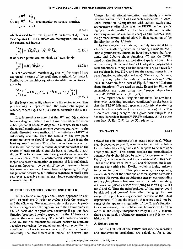
FIG. 1. Absolute errors in reflection (R=0.323 930 657) and transmission (T=0.676 069 343) coefficients for the Eckart barrier as a function of basis range. E=6.0 cm-‘, m=4.3 g/mol, D=lO.O cm-‘, cx=3.0 A-‘, and 20 DVR sine functions basis. Present method-(curve A) AR; (curve B) AT Miller’s method [Ref. l(b), using a smooth cut-off function]-(curve C) AR; (curve D) AT.

dimensional potential barrier, in particular, the Eckart barrier, and are compared with the exact analytical results. The Hamiltonian is given by

H=HlJ+ v,

H=Zd2 0 2mZ’ (3.2)

D v= cosh’(ax) ’

where the potential V is symmetric about the origin and v-*0 as X--rfco. Both of the two linearly independent solutions for Ho must be used in Eq. (2.9) since no boundary conditions are imposed except the asymptotic ones

I I 1 I I I I

0.0006 +, ....

. . 0.0004 - "...._

: ii

0.0002

a,

," 0

,o P -0.0002 m

-0.0004

-0.0006 t , , , , , , , 1

1.6 1.8 2 2.2 2.4 2.6 2.8 3 (basis range)/2 (Angstrom)

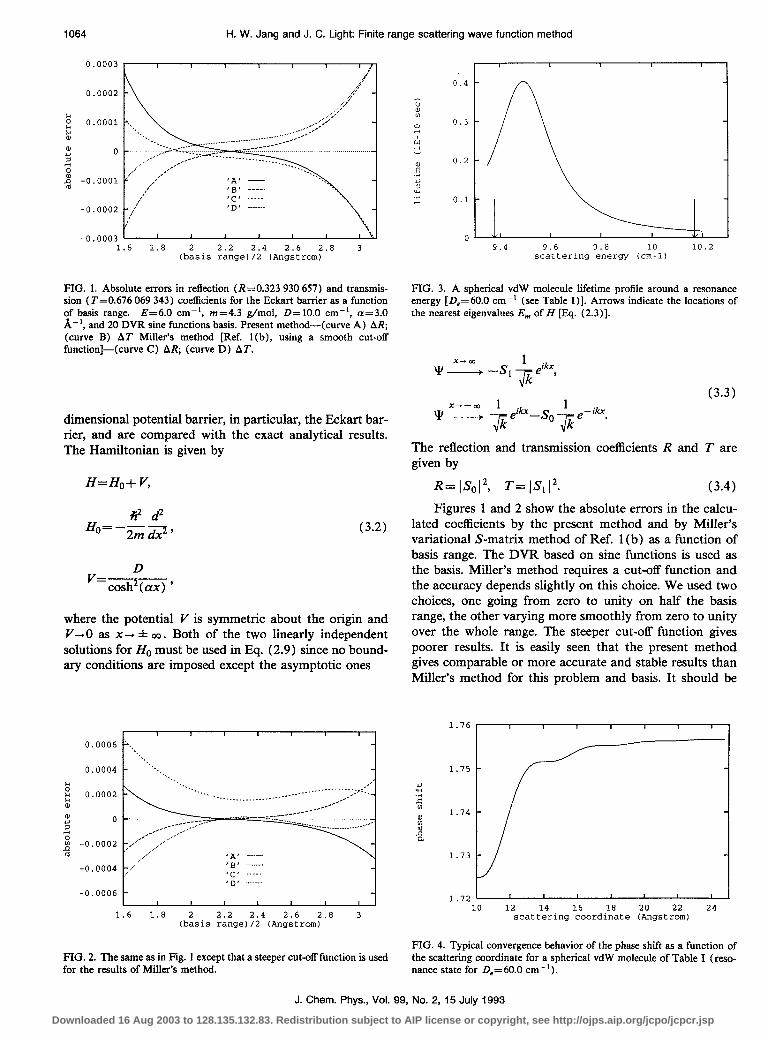
PIG. 2. The same as in Fig. 1 except that a steeper cut-off function is used for the results of Miller’s method.

*I’ ’ ’ ’ II 0.4 -

;; :

4: 0.3 -

IL "

: 0.2 -

.r(

ii .i i 0.1 -

n "' I I I 0 9.4 9.6 9.8 10 10.2

scattering energy (cm-l)

FIG. 3. A spherical vdW molecule lifetime profile around a resonance energy [D,=60.0 cm-’ (see Table I)]. Arrows indicate the locations of the nearest eigenvalues Em of H [Fq. (2.3)].

x-m Y-----+-s~ * ikx

3’ ’

x---m 1 ikx Y- qe -So$ewih.

(3.3)

The reflection and transmission coefficients R and T are given by

R= ISo12, T= IS112. (3.4) Figures 1 and 2 show the absolute errors in the calcu-

lated coefficients by the present method and by Miller’s variational S-matrix method of Ref. 1 (b) as a function of basis range. The DVR based on sine functions is used as the basis. Miller’s method requires a cut-off function and the accuracy depends slightly on this choice. We used two choices, one going from zero to unity on half the basis range, the other varying more smoothly from zero to unity over the whole range. The steeper cut-off function gives poorer results. It is easily seen that the present method gives comparable or more accurate and stable results than Miller’s method for this problem and basis. It should be

1 1.76 1 I I I I I 1

1.75 -

1.72 / I I , I I 1 10 12 14 16 18 20 22 24

scattering coordinate (Angstrom)

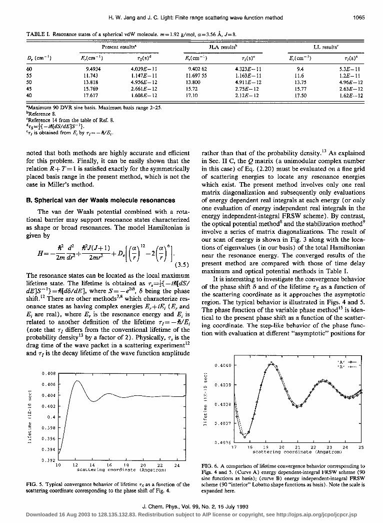
FIG. 4. Typical convergence behavior of the phase shift as a function of the scattering coordinate for a spherical vdW molecule of Table I (resonance state for D,=60.0 cm-‘).




TABLE I. Resonance states of a spherical vdW molecule. m= 1.92 g/mol, a= 3.56 A, J= 8.

Present results” JLA resultsb LL resultsC

De (cm-‘) E,(cm-‘) TsWd E,(cm-‘) T,bY E,(cm-‘) T,bY

60 9.4934 4.039E- 11 55 11.743 l.l47E-11 50 13.818 4.956E- 12 45 15.769 2.6613- 12 40 17.617 1.608E- 12

‘Maximum 90 DVR sine basis. Maximum basis range 2-25. bReference 8. ‘Reference 14 from the table of Ref. 8. drs=;{ -M[dS/dE]S- ‘}. ‘rI is obtained from E, by rl= -Pi/E,.

9.402 62 4.323E- 11 9.4 5.3E- 11 11.697 55 l.l63E--11 11.6 1.2E- 11 13.800 4.91 IE- 12 13.75 4.96E- 12 15.72 2.75E- 12 15.77 2.63E- 12 17.10 2.12E- 12 17.50 1.62E- 12

noted that both methods are highly accurate and efficient for this problem. Finally, it can be easily shown that the relation R + T= 1 is satisfied exactly for the symmetrically placed basis range in the present method, which is not the case in Miller’s method.

B. Spherical van der Waals molecule resonances

The van der Waals potential combined with a rotational barrier may support resonance states characterized as shape or broad resonances. The model Hamiltonian is given by

ri2 d2 #J(J+ 1) H=-2mz+2m12 +D.[ (;)12-2(;)6].

(3.5) The resonance states can be located as the local maximum lifetime state. The lifetime is obtained as ~~=f{ - ifi[dS/ dE]S- ‘} =+i[d&/dE], where S= -e2is, 6 being the phase shift.12 There are other methods7’8 which characterize resonance states as having complex energies E,+ iEi (E, and Ei are real), where E, is the resonance energy and Ei is related to another definition of the lifetime rl= -fi/Ei (note that rI differs from the conventional lifetime of the probability densityI by a factor of 2). Physically, 7s is the drag time of the wave packet in a scattering experiment12 and rI is the decay lifetime of the wave function amplitude

0.408 I I I I I t I

E” ,.. 0.398 z w 0.396 . . t I

rather than that of the probability density.13 As explained in Sec. II C, the Q matrix (a unimodular complex number in this case) of Eq. (2.20) must be evaluated on a fine grid of scattering energies to locate any resonance energies which exist. The present method involves only one real matrix diagonalization and subsequently only evaluations of energy dependent real integrals at each energy (or only one evaluation of energy independent real integrals in the energy independent-integral FRSW scheme). By contrast, the optical potential method’ and the stabilization method’ involve a series of matrix diagonalizations. The result of our scan of energy is shown in Fig. 3 along with the locations of eigenvalues (in our basis) of the total Hamiltonian near the resonance energy. The converged results of the present method are compared with those of time delay maximum and optical potential methods in Table I.

It is interesting to investigate the convergence behavior of the phase shift S and of the lifetime ~~ as a function of the scattering coordinate as it approaches the asymptotic region. The typical behavior is illustrated in Figs. 4 and 5. The phase function of the variable phase method15 is identical to the present phase shift as a function of the scattering coordinate. The step-like behavior of the phase function with evaluation at different “asymptotic” positions for

0.4036 ' I 1 a I I I , I 17 18 19 20 21 22 23 24 25


0.392 ' I I I I I 0 I 10 12 14 16 18 20 22 24


FIG. 5. Typical convergence behavior of lifetime rS as a function of the scattering coordinate corresponding to the phase shift of Fig. 4.

FIG. 6. A comparison of lifetime convergence behavior corresponding to Figs. 4 and 5. (Curve A) energy dependent-integral FRSW scheme (90 sine functions as basis); (curve B) energy independent-integral FRSW scheme (90 “interior” Lobatto shape functions as basis). Note the scale is expanded here.



TABLE II. Inelastic transition probability. E=6.0, m=0.667, (x=0.315, and Ye=24.0.

(A) Basis size”

Basis range

Present results MJH resultsb

5/22 5/24 5/26 Numerical 5/24’ integration

1-33 1-33 l-33 . . . . .

PO1 0.300 28E- 1 0.300 50E- 1 0.300 68E- 1 0.300 58E- 1 0.300 17E- 1 PI2 0.147 49E-2 0.147 25E-2 0.146 95E-2 0.147 23E-2 0.147 22E-2 PO2 0.112 83E-4 0.112 75E-4 0.112 59E-4 0.112 73E-4 0.114 95E-4 AU 2.76E- 5 1.9OE-5 2.33E-5 . . . . . .

(Wd Basis size 5/4O 6/45 7/70 2~7/36~ 2 x 7/37’ Basis range O-55 - l-56 - 3-63 - 3-68 - 3-66

PO1 0.301 291E- 1 0.301 308E- 1 0.301 308E- 1 0.301 309E- 1 0.301 309E- 1 PI2 0.146 783E-2 0.146 753E-2 0.146 756E- 2 0.146 7498-2 0.146 770E-2 PO2 0.112 8348-4 0.112 823E-4 0.112 825E-4 0.112 821E-4 0.112 836E-4 AU l.l6E-7 4.17E-8 5.04E- 10 2.26E- 7 1.2OE-7

aThe number of DVR harmonic oscillator eigenfunctions for internal vibration/number of DVR sine functions for translation. bReference 1 (a). ‘Variational S matrix using distorted waves. dPresent results. Note that the “7/70;-3-63” results are probably the most accurate presented for this problem, being converged apparently to five significant figures with relatively modest computational cost.

Two-sector wave function continuation. The whole range is divided into two equal size sectors as explained in Sec. II D. The 7/36 basis for each sector; two-point fit.

‘Two-sector wave function continuation. The whole range is divided into two equal size sectors. The 7/37 basis for each sector; four-point least squares fit.

low E is related to Levinson’s theorem for the number of bound states.15 Thus the less prominent step-like behavior at positive scattering energy of Fig. 4 could be a reminis- cence of it. The oscillating behavior of the lifetime in Fig. 5 as a function of the scattering coordinate is a direct con- sequence of the step-like behavior of the phase shift.

The energy independent-integral FRSW scheme [Eq. (2.11)] along with Gauss-Lobatto quadrature&‘) is used to calculate the resonance lifetime with the “interior” Lo- batto shape functions as basis, i.e., the basis is [ui(r);i = l,Nj excluding the “outer boundary” function uc( r), and the result is compared with the corresponding result of energy dependent-integral FRSW scheme (with sine functions as the basis) in Fig. 6 on a greatly expanded scale. The resonance lifetimes agree to five significant figures and the numerical results of the energy independent-integral scheme do not depend on the choice of the “arbitrary F” as long as it is a slowly varying smooth function, nonzero at the outer boundary.

C. Inelastic scattering and Feshbach resonances

In this section, a model Hamiltonian for one- dimensional inelastic scattering is considered. We solve for the transition probabilities between internal vibrational states and also for a model with Feshbach resonance states. For inelastic scattering, we use a standard model of vibrational excitations.16 The Hamiltonian is given by

H=&+ V(r,s), I+-;;+ 2 (-Z+q (36) V( r,s) = V&-a+s),

where V(r,s) -0 as r--s-+ CO. @ in Rq. (2.9) is given by a linear combination of

(3.7)

These Qj are eigenfunctions of He with the usual restric- tion on kj (Sec. II C) and r. is chosen such that Y(ro,s) is sufficiently large that Y essentially vanishes for r<ro. The transition probabilities are calculated for several sets of parameters and are listed in Tables II-IV with other published results for comparison. Since our S matrix is not initially symmetric (consequently pii may not be equal to pji) and unitary, we transform the S matrix following the scheme explained in Sec. II C and present the symmetric- orthogonalized results. It is interesting to note that the numerical integration results of Ref. 1 (a) are very close to the present results corresponding to a local minimum of the “unitarity error” AU for the basis coordinate range l-33 shown in Table II(A). Results of the wave function continuation scheme are also shown as the last two col- umns of Tables II-IV. Agreement with the exact results to four significant figures (of about six) is obtained in these trials. In each table, the last column represents a four-point least squares fit of the sector wave functions, while the next-to-last column gives the results of the minimum two- point fits. The least squares fits require only two extra points of overlap of the two regions and thus are computationally about equivalent. They appear to be somewhat more accurate from the limited tests. The regional parti- tioning is much more efficient computationally than the full domain diagonalization ( - a factor of 3 or more), and the results of these calculations, at least, are quite accurate



H. W. Jang and J. C. Light: Finite range scattering wave function method

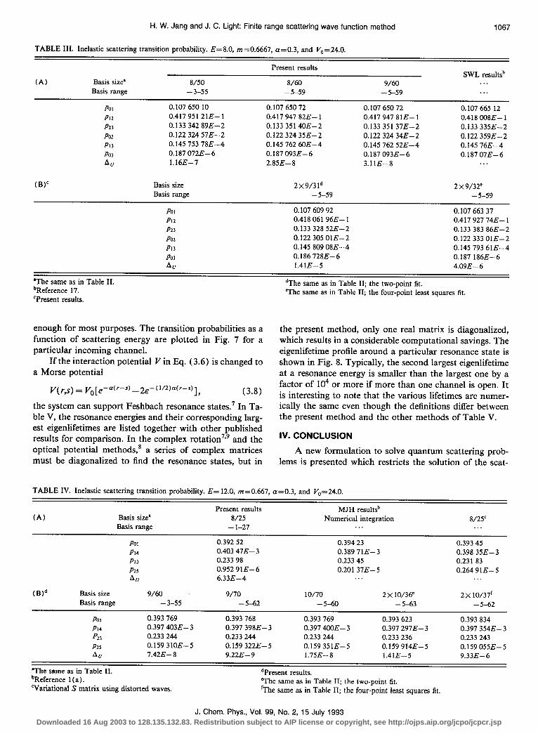
TABLE III. Inelastic scattering transition probability. E=8.0, m=0.6667, a=0.3, and V,=24.0.

1067

(A) Basis size’ Basis range

8/50 - 3-55

Present results

8/60 - 5-59

9/60 - 5-59

SWL resultsb . . . . .

Pot 0.107 650 10 0.107 650 72 0.107 650 72 0.107 665 12 PI2 0.417 951 21E- 1 0.417 947 82E- 1 0.417 947 81E- 1 0.418 008E- 1 P23 0.133 342 89E-2 0.133 3514OE-2 0.133 351 37E-2 0.133 335E-2 PO2 0.122 324 57E-2 0.122 324 35E-2 0.122 324 34E-2 0.122 359E-2 PI3 0.145 753 78E-4 0.145 762 6OE-4 0.145 762 52E-4 0.145 76E-4 PO3 0.187 072E- 6 0.187 093E-6 0.187 093E-6 O.l8707E-6 Art l.l6E-7 2.858-8 3.11E-8 . . .

(BY Basis size Basis range

PO1 PlZ P23

PO2

PI3

PO3

AU

2x9/31d 2 x 9/32= - 5-59 - 5-59

0.107 609 92 0.107 663 37 0.418 061 96E- 1 0.417 927 74E- 1 0.133 328 52E-2 0.133 383 868-2 0.122 305 OlE-2 0.122 333 OlE-2 0.145 809 08E-4 0.145 793 61E-4 0.186 728E-6 0.187 186E-6 1.41E-5 4.09E- 6

*The same as in Table II. ‘Reference 17. ‘Present results.

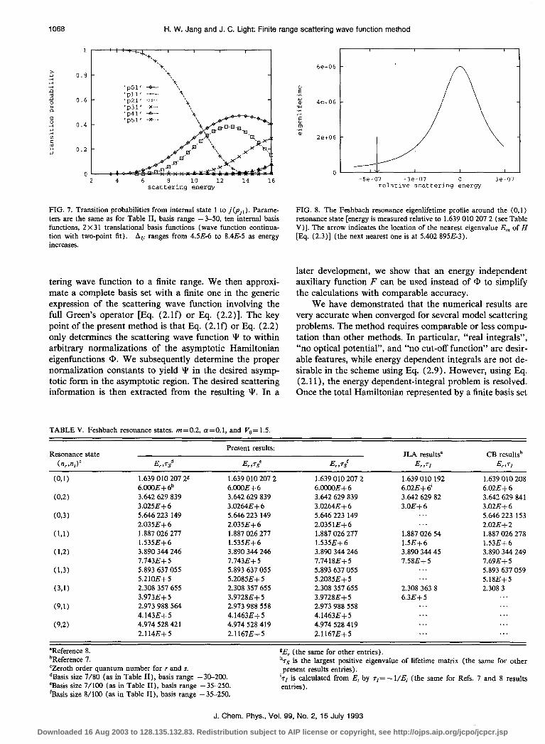
enough for most purposes. The transition probabilities as a function of scattering energy are plotted in Fig. 7 for a particular incoming channel.

If the interaction potential I’in ECq. (3.6) is changed to a Morse potential

v(r,s)= yo[e-a(r-s)_2e-(‘“)“(‘-S)], (3.8) the system can support Feshbach resonance states.’ In Ta- ble V, the resonance energies and their corresponding largest eigenlifetimes are listed together with other published results for comparison. In the complex rotation7’9 and the optical potential methods,* a series of complex matrices must be diagonalized to find the resonance states, but in

dThe same as in Table II; the two-point fit. @The same as in Table II; the four-point least squares lit.

the present method, only one real matrix is diagonalized, which results in a considerable computational savings. The eigenlifetime profile around a particular resonance state is shown in Fig. 8. Typically, the second largest eigenlifetime at a resonance energy is smaller than the largest one by a factor of lo4 or more if more than one channel is open. It is interesting to note that the various lifetimes are numerically the same even though the definitions differ between the present method and the other methods of Table V.

IV. CONCLUSION

A new formulation to solve quantum scattering problems is presented which restricts the solution of the scat-

TABLE IV. Inelastic scattering transition probability. E= 12.0, m=0.667, a=0.3, and Vo=24.0.

(A) Basis size’ Basis range

Present results 8/25

- l-27

MJH resultsb Numerical integration

. . . 8/25’

. . .

(Wd

Pot 0.392 52 0.394 23 0.393 45 PI4 0.403 47E-3 0.389 71E-3 0.398 35E-3 P23 0.233 98 0.233 45 0.231 83 Pl3 0.952 91E-6 0.201 37E-5 0.264 91E-5 AU 6.33E-4 . . . . . .

Basis size 9/60 9/70 IO/70 2x 10/36’ 2x 10/37’ Basis range -3-55 - 5-62 - 5-60 - 5-63 - 5-62

PO1 0.393 769 0.393 768 0.393 769 0.393 623 0.393 834 PI4 0.397 4038-3 0.397 398E-3 0.397 4CQE- 3 0.397 297E- 3 0.397 354E- 3 p23 0.233 244 0.233 244 0.233 244 0.233 236 0.233 243 P25 0.159 31OE-5 0.159 322E-5 0.159 351E-5 0.159 914E-5 0.159 055E-5 AU 7.42E- 8 9.22E- 9 1.75E-8 1.41E-5 9.33E--6

‘The same as in Table II. dPresent results. bReference 1 (a). ‘Variational S matrix using distorted waves.

The same as in Table II; the two-point fit. ‘The same as in Table II; the four-point least squares fit.



h .t: 3 .rl L, B E a c 2 .z z 2 4.l

1

0.8

0.6 4ec06

0.4

0.2

n

2e+06

0 2 4 6 8 10 12 14 16 -6e-07 -3e-07 0 3e-07

scattering energy relative scattering energy

FIG. 7. Transition probabilities from internal state 1 to j(p,,). Parame- ters are the same as for Table II, basis range -3-50, ten internal basis functions, 2 x 3 1 translational basis functions (wave function continuation with two-point fit). AU ranges from 4.5E-6 to 8.4E-5 as energy increases.

tering wave function to a finite range. We then approximate a complete basis set with a finite one in the generic expression of the scattering wave function involving the full Green’s operator [IQ. (2.lf) or Eq. (2.2)]. The key point of the present method is that Eq. (2.lf) or Eq. (2.2) only determines the scattering wave function Y to within arbitrary normalizations of the asymptotic Hamiltonian eigenfunctions a. We subsequently determine the proper normalization constants to yield Y in the desired asymptotic form in the asymptotic region. The desired scattering information is then extracted from the resulting Y. In a

TABLE V. Feshbach resonance states. m=0.2, a=O.l, and V,,= 1.5.

FIG. 8. The Feshbach resonance eigenlifetime profile around the (0,l) resonance state [energy is measured relative to 1.639 010 207 2 (see Table V)]. The arrow indicates the location of the nearest eigenvalue E,,, of H [Eq. (2.3)] (the next nearest one is at 5.402 895&3).

later development, we show that an energy independent auxiliary function F can be used instead of Cp to simplify the calculations with comparable accuracy.

We have demonstrated that the numerical results are very accurate when converged for several model scattering problems. The method requires comparable or less computation than other methods. In particular, “real integrals”, “no optical potential”, and “no cut-off function” are desir- able features, while energy dependent integrals are not de- sirable in the scheme using Eq. (2.9). However, using Eq. (2.11)) the energy dependent-integral problem is resolved. Once the total Hamiltonian represented by a finite basis set

Resonance state (n,,n,Y E,,Ts”

Present results:

E, ,TS’ E,,Ts’ JLA results” CB resultsb

E,,TI E,,TI

(091) 1.639 010 207 2s 1.639 010 207 2 1.639 010 207 2 1.639 010 192 1.639 010 208 6.OCOE+ 6’ 6.OOOE+ 6 6.mE+6 6.02E+ 6’ 6.02E+6

(02) 3.642 629 839 3.642 629 839 3.642 629 839 3.642 629 82 3.642 629 841 3.025E-k6 3.0264E+6 3.0264E+6 3.OE+6 3.02E+6

(0,3) 5.646 223 149 5.646 223 149 5.646 223 149 . . . 5.646 223 153 2.0356+6 2.035E+6 2.035lE+6 . . . 2.02E-k2

(Ll) 1.887 026 277 1.887 026 277 1.887 026 277 1.887 026 54 1.887 026 278 1.535E+6 1.535E+6 1.535E+6 1.5E+6 1.53E+6

(12) 3.890 344 246 3.890 344 246 3.890 344 246 3.890 344 45 3.890 344 249 7.743E+ 5 7.743E-k 5 7.74188+5 7.58E+5 7.696+5

(1,3) 5.893 637 055 5.893 637 055 5.893 637 055 . . . 5.893 637 059 5.210E+5 5.2085E+5 5.20856-f5 . . . 5.18E+5

(3,l) 2.308 357 655 2.308 357 655 2.308 357 655 2.308 363 8 2.308 3 3.9736-k 5 3.9728E-f 5 3.9728E+ 5 6.3E+5 . . .

(9,l) 2.973 988 564 2.973 988 558 2.973 988 558 . . . . . . 4.143E+5 4.1463E+ 5 4.1463E-k 5 . . . . . .

(9,2) 4.974 528 421 4.974 528 419 4.974 528 419 . . . . . . 2.114E+5 2.1167E+5 2.1167E+5 . . . . . .

“Reference 8. bReference 7. ‘Zeroth order quantum number for r and s. dBasis size 7/80 (as in Table II), basis range -30-200. ‘Basis size 7/100 (as in Table II), basis range - 35-250. ‘Basis size B/100 (as in Table II), basis range -35-250.

gEr (the same for other entries). hrs is the largest positive eigenvalue of lifetime matrix (the same for other present results entries).

ids is calculated from Ei by T,= - 1/Ei (the same for Refs. 7 and 8 results entries).



is diagonalized, the major part of work in the energy dependent-integral scheme consists of evaluating “Nopen X N&is)’ energy dependent real integrals at each scattering energy. This may be done conveniently by Gaussian quadratures. There then remain several smaller “Nopen by lvopen” matrix multiplications and inversions to get the final S-matrix scattering information. In the energy independent-integral scheme, the overlap integrals of F over the discrete eigenfunctions need to be evaluated only once instead of once at each energy. While an arbitrariness in the choice of F is introduced [Eq. (2.1 l)] formally, this is not a problem. Numerical calculations indicate that the results do not depend on the particular choice of F as long as it is a slowly varying smooth function (such as “extremely large period” sine functions or linear functions), nonzero at the outer boundary.

We also note that the computation times are modest for the FRSW approach, particularly in the energy independent-integral scheme. All calculations in this paper were carried out on workstations. Typically, computation times were roughly two times as long as required for the real L2 diagonalization in order to evaluate the S matrices or lifetimes at many ( 10-100) energies. The maximum L2 basis used was 800 for the highly accurate Feshbach resonance calculations of Table V which yielded resonance energies to at least nine significant figures.

A problem due to the zero boundary condition of the sine basis functions may cause trouble at energies at which @ is also zero at the boundary in the energy dependent- integral FRSW scheme. However, these problem energies are predictable analytically. This problem can also be resolved by simply using the energy independent-integral FRSW scheme with a properly chosen F.

The present method produces directly the scattering wave functions on a finite range satisfying the desired boundary conditions at any scattering energy. This makes it promising for other quantum mechanical problems involving scattering wave functions such as photodissociation. The time independent approach, such as close- coupling calculation, in photodissociation involves numerical solutions of the Schrddinger equation for each energy to find the scattering wave function. This could be found relatively easily in the present finite-basis FRSW scheme.

Finally, it should be pointed out that the S matrix and the coefficient matrix C can also be solved from the simultaneous equations obtained from the wave function and its coordinate derivative at one DVR point. Surprisingly, this approach shows poorer convergence behavior than that of Eq. (2.16). The approximation to dY/dr should be, following the spirit of Eq. (2.5),

y’(rj)= z --& (rjlm) ( m[ f (E-H)lYIa)

+@‘(rj), (4.1)

but the working approximation is


Y’(rj) = 2 m

& (rjIm)‘(~--&J-*(ml VI@>

+@‘(rj), (4.2)

which is obtained by differentiating Eq. (2.9) with respect to the scattering coordinate. The possibility that Eq. (4.2) is not an adequate approximation to Eq. (4.1) is the prob- able reason for the poor convergence.

ACKNOWLEDGMENTS

We appreciate useful discussions with Daniel Neu- hauser and David Brown. We especially thank David Brown for the help with Miller’s method for Eckart barrier problem. We acknowledge the support of the National Sci- ence Foundation grant NSF-CHE8806514 for this re- search.

’ (a) W. H. Miller and B. M. D. D. Jansen op de Harr, J. Chem. Phys. 86, 6213 (1987); (b) J. Z. H. Zhang, S.-I. Chu, and W. H. Miller, ibid. 88, 6233 (1988); (c) J. 2. H. Zhang and W. H. Miller, Chem. Phys. Lett. 140, 329 (1987); J. Chem. Phys. 88, 4549 (1989); Chem. Phys. Lett. 153,465 (1988); J. Chem. Phys. 91, 1528 (1989); J. Z. H. Zhang, ibid. 94, 6047 (1991).

‘(a) D. E. Manolopoulos and R. E. Wyatt, Chem. Phys. Lett. 152, 23 (1988); (b) 159, 123 (1988); D. E. Manolopoulos, M. D’Mello, and R. E. Wyatt, J. Chem. Phys. 91,6096 (1989); 93,403 (1990); M. D’Mello, D. E. Manolopoulos, and R. E. Wyatt, Chem. Phys. Lett. 168, 113 (1990).

3G. Staszewska and D. G. Truhlar, J. Chem. Phys. 86, 2793 (1987); J. Z. H. Zhang, D. J. Kouri, K. Haug, D. W. Schwenke, Y. Shima, and D. G. Truhlar, ibid. 88, 2492 (1988); K. Haug, D. W. Schwenke, D. G. Truhlar, Y. Zhang, J. Z. H. Zhang, and D. J. Kouri, ibid. 87, 1892 (1987); D. W. Schwenke, K. Haug, D. G. Truhlar, Y. Sun, J. Z. H. Zhang, and D. J. Kouri, J. Phys. Chem. 91, 6080 (1987); D. W. Schwenke, K. Haua. D. G. Truhlar. Y. Sun. J. Z. H. Zhane. and D. J. Kouri, J. Phys. Chem. 92, 3202 (1988); M.‘Zhao, M. Mladenovic, D. G. Truhlar, D. W. Schwenke, 0. Sharafeddin, Y. Sun, and D. J. Kouri, J. Chem. Phys. 91, 5302 (1989).

4R. G. Newton, Scattering Theory of Waves and Particles, 2nd ed. (Springer, New York, 1982).

5(a) Z. Darakjian, E. F. Hayes, G. A. Parker, E. A. Butcher, and J. D. Kress, J. Chem. Phys. 95, 2516 (1991); (b) F. T. Smith, Phys. Rev. 118, 349 (1960).

‘A. Szabo and N. S. Ostlund, Modern Quantum Chemistry (Macmillan, New York, 1982).

‘K. M. Christoffel and J. M. Bowman, J. Chem. Phys. 78, 3952 (1983). 8G. Jolicard, C. Leforestier, and E. J. Austin, J. Chem. Phys. 88, 1026

(1988). 9V. A. Mandelshtam, T. R. Ravuri, and H. S. Taylor, Phys. Rev. Lett.

70, 1932 (1993): B. R. Junker, Adv. At. Mol. Phvs. 18.207 ( 1982): C. W. McCurdy and T. N. Rescigno, Phys. Rev. A il, 1499 (1980); B: R. Johnson and W. P. Reinhardt, ibid. 29, 2933 (1984); N. Moiseyev, Mol. Phys. 47, 585 (1982).

‘OS E Choi and J. C. Light, J. Chem. Phys. 92, 2129 (1990); J. V. Lill, . . G. A. Parker, and J. C. Light, Chem. Phys. Lett. 89,483 (1982); J. C. Light, R. M. Whitnell, T. J. Park, and S. E. Choi, in NATO ASZ Series C, edited by A. Lagana (Kluwer, Dordrecht, 1989), Vol. 277, pp. 187- 214.

“Handbook of Mathmatical Functions, edited by M. Abramowitz and A. Stegun (Dover, New York, 1972).

“5. R. Taylor, Scattering Theory (Wiley, New York, 1972). 13L D Landau and E. M. Lifshitz, Quantum Mechanics (Non-Relativistic . .

Theory), 3rd ed. (Pergamon, Oxford, 1977). 14R. J. Le Roy and W.-K. Liu, J. Chem. Phys. 69, 3622 (1978). “F. Calogero, Variable Phase Approach to Potential Scattering (Aca-

demic, New York, 1967). 16D &crest and B. R. Johnson, J. Chem. Phys. 45,4556 (1966). 17E’ B. Stechel, R. B. Walker, and J. C. Light, J. Chem. Phys. 69, 3518

(i978).


Finite range scattering wave function method for ...

Documents

Transcript of Finite range scattering wave function method for ...