FINITE ELEMENT SIMULATION OF CRACK PROPAGATION...
104
Transcript of FINITE ELEMENT SIMULATION OF CRACK PROPAGATION...

FINITE ELEMENT SIMULATION OF CRACK PROPAGATION FOR STEELFIBER REINFORCED CONCRETE
A THESIS SUBMITTED TOTHE GRADUATE SCHOOL OF CIVIL ENGINEERING
OFMIDDLE EAST TECHNICAL UNIVERSITY
BY
KAAN OZENC
IN PARTIAL FULFILLMENT OF THE REQUIREMENTSFOR
THE DEGREE OF MASTER OF SCIENCEIN
CIVIL ENGINEERING
JULY 2009
Approval of the thesis:
FINITE ELEMENT SIMULATION OF CRACK PROPAGATION FOR STEEL
FIBER REINFORCED CONCRETE
submitted byKAAN OZENC in partial fulfillment of the requirements for the degreeof Master of Science in Civil Engineering Department, Middle East TechnicalUniversity by,
Prof. Dr. CananOzgenDean, Graduate School ofNatural and Applied Sciences
GuneyOzcebeHead of Department,Civil Engineering
Assoc. Prof. Dr.Ismail Ozgur YamanSupervisor,Civil Engineering Department, METU
Assoc. Prof. Dr. Serkan DagCo-supervisor,Mechanical Engineering Department, METU
Examining Committee Members:
Prof. Dr. Mustafa TokyayCivil Engineering, METU
Assoc. Prof. Dr.Ismail Ozgur YamanCivil Engineering, METU
Assoc. Prof. Dr. Serkan DagMechanical Engineering, METU
Assoc. Prof. Dr. Barıs BiniciCivil Engineering, METU
Asst.Prof.Dr. Sinan Turhan ErdoganCivil Engineering, METU
Date:

I hereby declare that all information in this document has been obtained andpresented in accordance with academic rules and ethical conduct. I also declarethat, as required by these rules and conduct, I have fully cited and referenced allmaterial and results that are not original to this work.
Name, Last Name: KAANOZENC
Signature :
iii
ABSTRACT
FINITE ELEMENT SIMULATION OF CRACK PROPAGATION FOR STEELFIBER REINFORCED CONCRETE
Ozenc, Kaan
M.S., Department of Civil Engineering
Supervisor : Assoc. Prof. Dr.Ismail Ozgur Yaman
Co-Supervisor : Assoc. Prof. Dr. Serkan Dag
July 2009, 90 pages
Steel fibers or fibers in general are utilized in concrete to control the tensile cracking
and to increase its toughness. In literature, the effects of fiber geometry, mechanical
properties, and volume on the properties of fiber reinforcedconcrete have often been
experimentally investigated by numerous studies. Those experiments have shown that
useful improvements in the mechanical behavior of brittle concrete are achieved by
incorporating steel fibers. This study proposes a simulation platform to determine
the influence of fibers on crack propagation and fracture behavior of fiber reinforced
concrete. For this purpose, a finite element (FE) simulationtool is developed for the
fracture process of fiber reinforced concrete beam specimens subjected to flexural
bending test.
Within this context, the objective of this study is twofold.The first one is to investi-
gate the effects of finite element mesh size and element type on stress intensity factor
(SIF) calculation through finite element analysis. The second objective is to develop
a simulation of the fracture process of fiber reinforced concrete beam specimens.
iv

The properties of the materials, obtained from literature,and the numerical simulation
procedure, will be explained. The effect of fibers on SIF is included by unidirectional
elements with nonlinear generalized force-deflection capability. Distributions and
orientation of fibers and possibility of anchorage failure are also added to simulation.
As a result of this study it was observed that with the adoptedsimulation tool, the
load-deflection relation obtained by experimental studiesis predicted reasonably.
Keywords: Concrete, steel fiber, finite element, fracture mechanics, crack propaga-
tion
v
OZ
SONLU ELEMANLAR YONTEMIYLE CELIK L IFLI BETONDA CATLAKILERLEME SIMULASYONU
Ozenc, Kaan
Yuksek Lisans,Insaat Muhendisligi Bolumu
Tez Yoneticisi : Doc. Dr.Ismail Ozgur Yaman
Ortak Tez Yoneticisi : Doc. Dr. Serkan Dag
Temmuz 2009, 90 sayfa
Celik veya diger cesit lifler, betonun cekme catlaklarını kontrol etmek ve betonun
toklugunu artırmak icin kullanılır. Celik liflerin geometrilerinin, miktarlarının ve
mekanikozelliklerinin celik lifli betonuzerindeki etkisi sayısız calısmayla incelenmistir.
Bu calısmalar fiberlerin betonda kullanılmasının betonunmekanikozelliklerine olumlu
etki ettiklerini gostermistir. Bu calısma fiberlerin catlak ilerleyisine etkisini ve celik
lifli betonun kırılma davranısını tanımlayan bir simulasyon platformuonermektedir.
Bu amacla, egilme testi altındaki celik lifli betonun kırılma ilerleyisi icin sonlu ele-
manlar simulasyonu gelistirilmistir.
Bu baglamda, bu calısmanın amacı iki kategoriye ayrılmıstır. Birincisi, sonlu eleman-
lar yonteminde kullanılanorgu (mesh) buyuklugunun ve sonlu elemanozelliklerinin
kırılma toklugu carpanıuzerindeki etkisinin incelenmesidir.Ikinci amac ise celik lifli
beton kirislerin kırılma ilerleyisi icin bir simulasyon gelistirilmesidir.
Malzemeozellikleri dahaonceki deneysel calısmalardan elde edilen yayınlardan alınmıstır.
Liflerin kırılma toklugu carpanıuzerindeki etkisi tek yonlu dogrusal olmayan eleman-
vi
lar kullanılarak ve yuk-deplasman (yer degistirme) kapasiteleri goz onune alınarak
simulasyona dahil edilmistir. Ayrıca liflerin dagılım ve sıyrılma olasılıkları da istatis-
tiksel olarak simulasyona dahil edilmistir.
Bu calısmanın sonucunda uyarlanmıs simulasyon aracı kullanılarak elde edilen ver-
ilerin yuk-deplasman iliskisi acısından deneysel calısmalardan elde edilen verilerle
kabul edilebilirolcude uyustugu gozlenmistir.
Anahtar Kelimeler: Beton, celik lif, sonlu elemanlar, kırılma mekanigi, catlak ilerleyisi
vii
ACKNOWLEDGMENTS
This thesis was conducted under the supervision of Assoc. Prof. Dr. Ismail Ozgur
Yaman and Assoc. Prof. Dr. Serkan Dag. I would like to express my sincere ap-
preciation for the support, encouragement, guidance and insight they have provided
throughout the thesis.
viii
ix
TABLE OF CONTENTS
PLAGIARISM ............................................................................................................ iii
ABSTRACT ................................................................................................................ iv
ÖZ ............................................................................................................................... vi
ACKNOWLEDGMENTS ........................................................................................ viii
TABLE OF CONTENTS ............................................................................................ ix
LIST OF FIGURES .................................................................................................... xi
LIST OF TABLES .................................................................................................... xiii
CHAPTERS
1 INTRODUCTION ................................................................................................ 1
1.1 History of Fracture Mechanics ..................................................................... 1
1.2 Objectives ..................................................................................................... 2
1.3 Scope............................................................................................................. 3
2 LITERATURE REVIEW AND BACKGROUND .............................................. 5
2.1 Introduction to Fracture Mechanics .............................................................. 5
2.2 General Principles of Linear Elastic Fracture Mechanics (LEFM)
Approach ........................................................................................................ 7
2.2.1 Stress Analysis Approach ..................................................................... 7
2.2.2 Energy Analysis Approach ................................................................. 15
2.2.3 Relationship between Stress Intensity Factor & Energy Release
Rate ..................................................................................................... 18
2.3 General Principles of Nonlinear Elastic Fracture Mechanics (NLEFM)
Approach ...................................................................................................... 19
2.4 Fracture Mechanics of Concrete ................................................................. 24
2.4.1 Fictitious Crack Approach .................................................................. 24
2.4.2 Effective-Elastic Crack Approach ...................................................... 28
2.5 Finite Element Analysis of Fracture Mechanics Properties ....................... 34
2.5.1 Finite Element Modeling of Singularities ........................................... 34
x
2.5.2 Calculation of Stress Intensity Factor Using Finite Element
Method ................................................................................................ 38
2.5.3 The Main Feature and Hypothesis of Finite Element Analysis of
Fracture in Concrete ........................................................................... 41
3 INTRINSIC PARAMETERS OF FINITE ELEMENT ANALYSIS OF
FRACTURE .......................................................................................................... 47
3.1 The Issue of Stability of Crack Propagation ............................................... 47
3.2 Finite Element Size and Types of Elements ............................................... 50
4 CRACK PROPAGATION SIMULATION FOR STEEL FIBER REINFORCED
CONCRETE .......................................................................................................... 57
4.1 Material Properties and Finite Element Types. .......................................... 57
4.2 Fiber Orientation Factor ............................................................................. 62
4.3 Possibility of Pull Out ................................................................................. 64
4.4 Finite Element Analysis .............................................................................. 65
5 SUMMARY AND CONCLUSIONS ................................................................. 72
5.1 Summary ..................................................................................................... 72
5.2 Conclusions ................................................................................................ 72
5.3 Recommendations for Future Studies ......................................................... 73
REFERENCE ........................................................................................................ 75
APPENDIX A ....................................................................................................... 79
xi
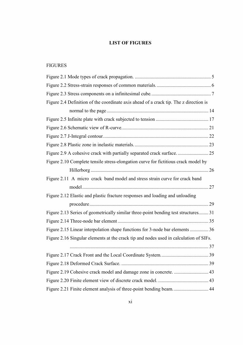
LIST OF FIGURES
FIGURES
Figure 2.1 Mode types of crack propagation. .............................................................. 5
Figure 2.2 Stress-strain responses of common materials. ............................................ 6
Figure 2.3 Stress components on a infinitesimal cube. ................................................ 7
Figure 2.4 Definition of the coordinate axis ahead of a crack tip. The z direction is
normal to the page ................................................................................... 14
Figure 2.5 Infinite plate with crack subjected to tension ........................................... 17
Figure 2.6 Schematic view of R-curve. ...................................................................... 21
Figure 2.7 J-Integral contour. ..................................................................................... 22
Figure 2.8 Plastic zone in inelastic materials. ............................................................ 23
Figure 2.9 A cohesive crack with partially separated crack surface. ......................... 25
Figure 2.10 Complete tensile stress-elongation curve for fictitious crack model by
Hillerborg ................................................................................................ 26
Figure 2.11 A micro crack band model and stress strain curve for crack band
model ....................................................................................................... 27
Figure 2.12 Elastic and plastic fracture responses and loading and unloading
procedure ................................................................................................. 29
Figure 2.13 Series of geometrically similar three-point bending test structures. ....... 31
Figure 2.14 Three-node bar element .......................................................................... 35
Figure 2.15 Linear interpolation shape functions for 3-node bar elements ............... 36
Figure 2.16 Singular elements at the crack tip and nodes used in calculation of SIFs.
................................................................................................................. 37
Figure 2.17 Crack Front and the Local Coordinate System. ...................................... 39
Figure 2.18 Deformed Crack Surface. ....................................................................... 39
Figure 2.19 Cohesive crack model and damage zone in concrete. ............................ 43
Figure 2.20 Finite element view of discrete crack model. ......................................... 43
Figure 2.21 Finite element analysis of three-point bending beam. ............................ 44

xii
Figure 2.22 General review of stress distribution in fictitious crack model .............. 45
Figure 2.23 Triaxial stresses in the FPZ and its nonlocal behavior in reinforced
concrete. .................................................................................................. 46
Figure 3.1 Mesh refinements with 20, 40, and 80 elements at fracture face ............. 48
Figure 3.2. Dimensionless load versus midpoint deflection curves for beams
analyzed by Carpinteri ............................................................................ 49
Figure 3.3 4-node “plane42” elements of ANSYS. ................................................... 51
Figure 3.4 High order 8-node “plane82” elements of ANSYS .................................. 51
Figure 3.5 Mesh resolutions of three-point bending specimen. ................................. 51
Figure 3.6 Relationship between SIF and thickness. ................................................. 53
Figure 3.7 Three-point bending test procedure. ......................................................... 53
Figure 4.1 Experimental three-point bending test beam ............................................ 58
Figure 4.2 Gopalaratnam and Shah’s strain softening model .................................... 58
Figure 4.3 Pull out experiment of steel fibers ............................................................ 60
Figure 4.4 Slip-Load curve for crimped-shape steel fiber ......................................... 61
Figure 4.5 Behavior and inputs for COMBIN39 type of element.............................. 61
Figure 4.6 Orientation factor with various cross-sectional dimensions. ................... 63
Figure 4.7 Different conditions with four boundaries ................................................ 63
Figure 4.8 Probability of pull out failure ................................................................... 65
Figure 4.9 Flow chart for fracture process testing of steel fiber reinforced concrete. 66
Figure 4.10 Crack Propagation Steps. ........................................................................ 67
Figure 4.11 Load–deflection curves for fiber reinforced concrete beams Vf = 1.0.... 69
Figure 4.12 Load–deflection curves for fiber reinforced concrete beams Vf = 1.5.... 69
Figure 4.13 Load–deflection curve for fiber reinforced concretes and plain
concrete ................................................................................................... 70
Figure 4.14 Load–deflection curve for various fiber contents. .................................. 71
Figure A.1 Mesh resolution according to 10 elements at fracture surface................. 79
Figure A.2 Mesh resolution according to 20 elements at fracture surface................. 81
Figure A.3 Mesh resolution according to 40 elements at fracture surface................. 83
Figure A.4 Mesh resolution according to 13 elements at fracture surface................. 85
Figure A.5 Mesh resolution according to 23 elements at fracture surface................. 87
Figure A.6 Mesh resolution according to 43 elements at fracture surface................. 89
xiii
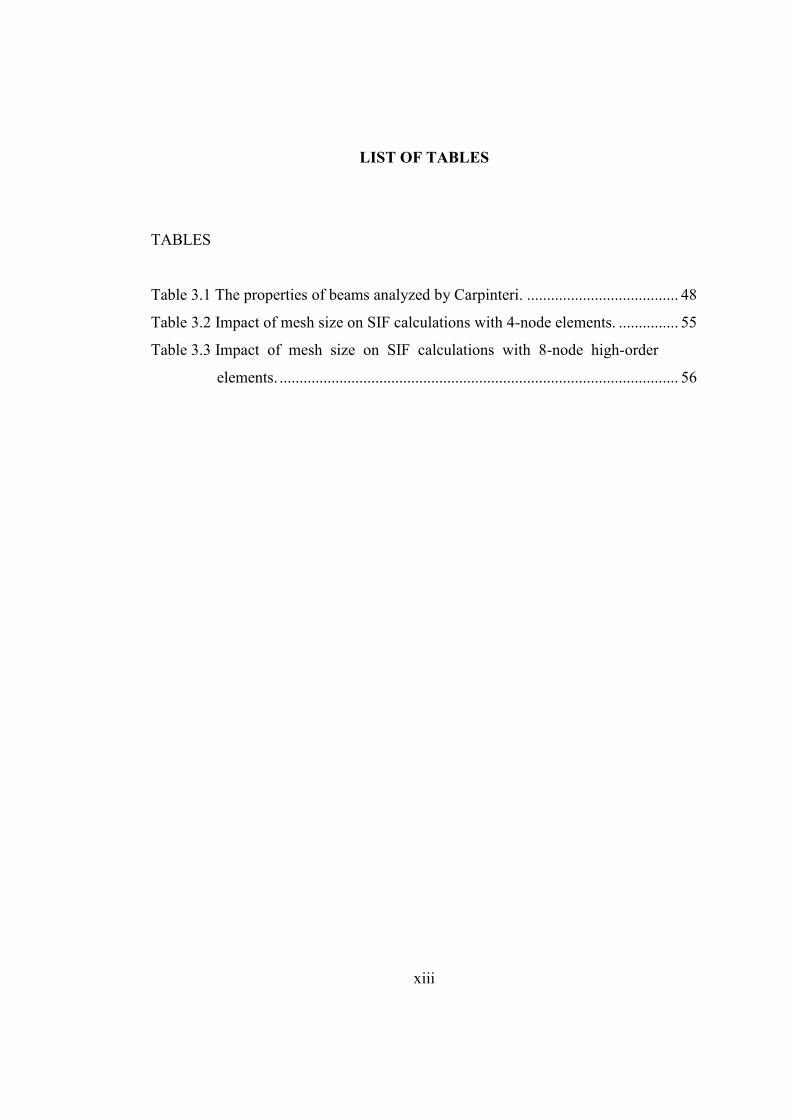
LIST OF TABLES
TABLES
Table 3.1 The properties of beams analyzed by Carpinteri. ...................................... 48
Table 3.2 Impact of mesh size on SIF calculations with 4-node elements. ............... 55
Table 3.3 Impact of mesh size on SIF calculations with 8-node high-order
elements. .................................................................................................... 56
1
CHAPTER 1
INTRODUCTION
1
1.1 History of Fracture Mechanics
The field of fracture mechanics has focused on the estimation and prevention of
fracture as a scientific discipline since the middle of the 20th
century. In 1921,
Griffith attempted to explain the large difference between the theoretical and
measured tensile strength of glass. He attributed the large discrepancies to high
stresses in the neighborhood of micro cracks and developed a theory of brittle failure
based on fracture mechanics.
The study of fracture mechanics of concrete originated in 1961 with Kaplan (Kaplan,
1961). A very different fracture mechanics theory is needed for concrete compared to
that of homogeneous structural materials and Kesler et al. concluded in 1972 that
classical linear elastic fracture mechanics was inapplicable to concrete (Kesler et al.,
1972). At least two fracture parameters are needed. In 1976, development of the
crack band model was recognized by Bažant in which the fracture properties are
characterized by the simple slope of the post peak strain softening tied to a certain
characteristic width of the crack band front (Bažant, 1976).
A major improvement was made by Hillerborg et al. who introduced the fictitious
crack model to concrete, in which the initial slope of the softening area under the
stress–separation curve, together with the tensile strength, implies two fracture
parameters of the material (Hillerborg et al., 1976). Two parameters were
subsequently used in Jenq and Shah’s “two-parameter model” (Jenq and Shah, 1985).
Similarly, Karihaloo and Nallathambi used two parameters in their “effective crack
model” (Karihaloo and Nallathambi, 1989).
2
The most important attribute of fracture mechanics of concrete is the size effect.
Although it was widely believed until the mid-1980s that all the size effects were of
statistical origin, and should therefore be relegated to statisticians, in 1969 Leicester
suggested that the size effect may originate from fracture mechanics of concrete.
Failures caused by fracture were numerically simulated with the crack band model
and were described in 1984 by Bažant by a simple size effect formula (Bažant,
1984).
Parallel analysis showed that the fracture model based on the size effect law by
Bažant and the Jenq–Shah’s “two parameter model” results in about the same size
effect and, therefore, are approximately equivalent. Likewise, Karihaloo and
Nallathambi’s model was shown to be approximately equivalent to “two parameter
model”, and thus to the size effect model.
Steel fibers or fibers in general are utilized in concrete to increase its toughness and
load-carrying capacity after cracking. In literature, the effects of fiber geometry,
mechanical properties, and volume on the properties of fiber reinforced concrete
have often been experimentally investigated. The mechanical response of fiber
reinforced concrete is thoroughly influenced by fiber-matrix interface, which is
usually evaluated by a pullout test of fibers. This study proposes a simulation
platform to determine the influence of fibers on crack propagation and fracture
behavior of fiber reinforced concrete.
1.2 Objectives
The goal of this thesis is to develop a finite element simulation tool for the fracture
process of fiber reinforced concrete beam specimens subjected to flexural bending
test. Within this context, the object of this study is twofold. The first one is to
investigate the effects of finite element mesh size and element type on stress intensity
factor (SIF) calculation through finite element analysis. After determining the effects
of mesh size and element type, the second objective is the simulation of the fracture

3
process of fiber reinforced concrete beam specimens. The concrete is modeled as a
homogenous linearly elastic material. The pull out behavior of the fibers is modeled
as link elements with nonlinear properties obtained from literature. During the FE
analysis, critical SIF is used as a crack propagation criterion.
1.3 Scope
Experiments have showed that useful improvements in the mechanical behavior of
brittle concrete are achieved by incorporating steel fibers. Numerous approaches
have been developed to simulate experimental tests via numerical models. This study
will investigate a simulation platform to determine the influence of fibers on crack
propagation and fracture behavior of concrete. For this purpose, fracture behavior
process will be simulated with the finite element method (FEM).
This thesis consists of five chapters. Chapter 2, Literature Review and Background,
provides the brief foundations of the present study. Within this context the
procedures of the two analyses, namely the approach of stress and energy analyses,
of linear elastic fracture mechanics (LEFM) are described. After LEFM, general
principles of nonlinear elastic fracture mechanics (NLEFM) are taken into
consideration. Later, the concepts related to fracture mechanics of concrete are
covered. Finally, in the last section of this chapter, subjects related to finite element
applications of fracture mechanics are briefly explained.
In Chapter 3, the efficiency of meshing and element type is thoroughly investigated
by comparing finite element solutions and hand book calculations of stress intensity
factor.
In Chapter 4, Analytical Study of Crack Propagation of Steel Fiber Reinforced
Concrete, the probability work for steel fibers’ orientation and pull out properties are
identified. The foundations of steel fiber models for the FE simulations are also built

4
in this chapter. Finally, the analysis of a fiber reinforced concrete beam is performed
and the obtained results are compared to experimental tests.
In the final chapter, the findings of the research whose goals have been mentioned in
the initial chapter are stated and comments on prospective studies are presented.
5
CHAPTER 2
LITERATURE REVIEW AND BACKGROUND
2
2.1 Introduction to Fracture Mechanics
As mentioned in the previous chapter, going back to the mid 20th century, George R.
Irwin and his co-workers developed a new fracture theory. Irwin’s generalization of
the Griffith argument for an energy-related fracture criterion provided a more
comprehensive theory of fracture. With this generalized theory, Irwin described the
terms G (energy absorbed by unit crack progress) and K (stress intensity factor)
which are used in fracture mechanics to predict the stress intensity near the tip of a
crack caused by a remote load or residual stresses more accurately. The underlying
idea is that when the stress state in a crack tip becomes critical, a small crack grows
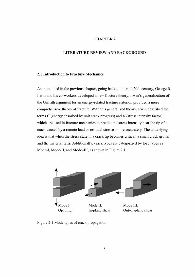
and the material fails. Additionally, crack types are categorized by load types as
Mode-I, Mode-II, and Mode–III, as shown in Figure 2.1
Figure 2.1 Mode types of crack propagation.
6
Mode-I is an opening mode where the crack surfaces move apart because of a tensile
load. Mode-II is a sliding mode where crack surfaces slide over one another in a
direction perpendicular to the edge of crack. Mode-III is a tearing mode where the
crack surfaces move relative to one another and parallel to the edge of crack
(Sanforld, 2002). Since a Mode-I type of crack is the most common type in
engineering applications, in this study, only Mode-I is investigated.
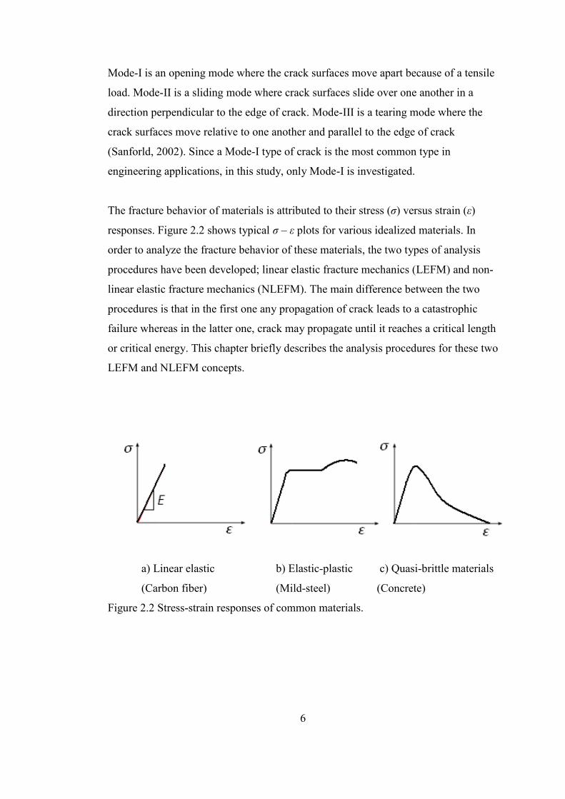
The fracture behavior of materials is attributed to their stress (ζ) versus strain (ε)
responses. Figure 2.2 shows typical ζ – ε plots for various idealized materials. In
order to analyze the fracture behavior of these materials, the two types of analysis
procedures have been developed; linear elastic fracture mechanics (LEFM) and non-
linear elastic fracture mechanics (NLEFM). The main difference between the two
procedures is that in the first one any propagation of crack leads to a catastrophic
failure whereas in the latter one, crack may propagate until it reaches a critical length
or critical energy. This chapter briefly describes the analysis procedures for these two
LEFM and NLEFM concepts.
a) Linear elastic b) Elastic-plastic c) Quasi-brittle materials
(Carbon fiber) (Mild-steel) (Concrete)
Figure 2.2 Stress-strain responses of common materials.
7
2.2 General Principles of Linear Elastic Fracture Mechanics (LEFM) Approach
2.2.1 Stress Analysis Approach
In order to introduce the linear elastic fracture mechanics concept, there arises a need
for the introduction of the concept of general linear stress and strain relationship.
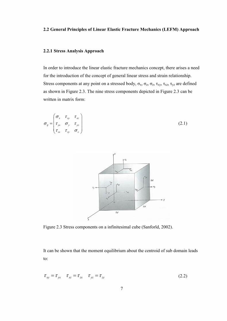
Stress components at any point on a stressed body, σx, σz, σz, τxy, τxz, τyz are defined
as shown in Figure 2.3. The nine stress components depicted in Figure 2.3 can be
written in matrix form:
x xy xz
ij yx y yz
zx zy z
(2.1)
Figure 2.3 Stress components on a infinitesimal cube (Sanforld, 2002).
It can be shown that the moment equilibrium about the centroid of sub domain leads
to:
xy yx xz zx yz zy (2.2)
8
For the same body, the strain components are related to the displacement components
of the body as:
x
y
z
u
x
v
y
w
z
(2.3)
xy
xz
yz
v u
x y
w u
x z
w v
y z
(2.4)
where u, v, w are the displacements in the coordinate directions x, y, z respectively.
The strain components can also be assembled in matrix form as presented in
Equation 2.5:
2 2
2 2
2 2
xy xzx
xy yz
ij y
yzxzz
(2.5)
When the generalized Hooke’s law is employed to model linear elastic and isotropic
materials, in the three-dimensional Cartesian coordinate system, the relationship
between stress and strain has the form:
9
1
1
1
x x y z
y y x z
z z x y
E
E
E
(2.6)
1
1
1
xy xy
xz xz
yz yz
S
S
S
(2.7)
Where E is the Young’s modulus, υ is Poisson’s ratio, and S is the shear modulus.
Fracture mechanics mostly deals with two-dimensional problems, in which the
stresses and body forces are independent of one of the coordinates, here taken as z.
Two-dimensional problems are of two classes. The first is plane stress problems in
which the stresses in the z direction are zero as seen in Equation 2.8.
0zz zx zy (2.8)
The second is plane strain problems where thickness is large. In this case, the strains
towards z direction are small enough that they can be assumed to be zero.
0zz zx zy (2.9)
For the infinitesimal body which is under the plane stress or strain condition, the
equilibrium condition is expressed as follows:
0xF (2.10)
0xyxx
x xx xy xx xyF dx dydz dy dxdz dydz dxdzx y
10
0xyxx dxdydz dydxdz
x y
(2.11)
0xyxx
x y
(2.12)
Similarly, for force components towards y direction, a similar expression can be
deducted:
0 0xy yy
Fyx y
(2.13)
when the two-dimensional case is taken in to consideration. Shear strain in the x-y
plane are expressed in terms of the displacements u and v, respectively:
xy
u v
y x
(2.14)
As the three strain components cannot be independent, an extra relation must exist
between them. This relation is the compatibility equation of strain, and is obtained by
eliminating u and v through differentiation of Equations 2.3 and 2.14.
2 2 2
2 2
xy u v
y x y x x y
(2.15)
2 22
2 2
xy yyxx
y x y x
(2.16)
Since;2
xy
xy
;
2 22
2 22
xy yyxx
y x y x
(2.17)
11
For plane elasticity problems, the stress field ahead of a crack tip problem must
satisfy all equilibrium requirements. As a particular technique is used in differential
equations, the aim is to construct a general function that satisfies the partial
differential equations. The same technique is used in the solution of the stress field
ahead of the crack problems, except for the general function which is called Airy's
Stress Function. According to Airy's stress function, equations can be described as:
2
2xxy
(2.18a)
2
2yyx
(2.18b)
2
xyx y
(2.18c)
where Φ qualifies as an Airy stress function, it must fulfill the biharmonic equation.
Because strain components can be written as the functions of stresses, Equation 2.17
can be formed by the combination of stress function in Equation 2.18 as follows:
4 4 44
4 2 2 42 0 0or
y y x x
(2.19)
Two different complex variable methods have been used into the formulation of the
two-dimensional elasticity problems: the first approach was introduced by Goursat-
Kolosov and then it was modified by Muskhelishvili. Despite the fact that this
approach has been widely used to solve singular problems, it is mathematically very
demanding. However, another complex-variable method which is used only for
straight crack problems, offers mathematical simplicity. This approach was
introduced in 1939 by Westergaard. Originally, this method could be applied only to
infinite body problems under remote stress condition (Shah et al., 1995). The method
was modified in 1966 by Sih and again in 1972 by Eftis and Liebowitz (Eftis, 1972).
To accommodate unequal remote biaxial loads, the method still had restricted
applications. Fortunately, the Goursat-Kolosov representation of the Airy stress-
12
function for planar crack problems was connected with Westergaard notation. The
new method is now suitable for all infinite and finite body problems with arbitrary
boundary conditions.
The principle behind this is that all analytic functions are potential Airy stress
functions. A function is analytic and Airy stresses function only if it satisfies the
following condition:
Re ImIm
Z ZZ
y x
(2.20a)
Im ReRe
Z ZZ
y x
(2.20b)
The equations are also known as Cauchy-Riemann relations. The prime superscript
symbolizes differentiation with respect to the complex variable z. According to these
relationships, the real and imaginary parts of Airy stress-functions can be separated
independently. Consider an Airy stress function of the form:
( ) Re ( ) Im ( ) Im ( )z Z z y Z z Y z (2.21)
where;
(2.22)
The Airy stress function from equation 2.21 can be used to solve the Cartesian stress
components which are obtained from an Airy stress function through the second
derivatives in respect to the real variables x, and y (Equation 2.19) via Cauchy-
Riemann relations.
dZZ
dz
dZZ
dz
dYY
dz
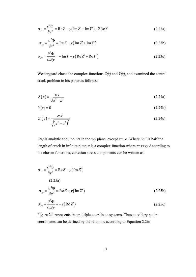
13
2
2Re Im Im 2Rexx Z y Z Y Y
y
(2.23a)
2
2Re Im Imyy Z y Z Y
x
(2.23b)
2
Im Re Rexy Y y Z Yx y
(2.23c)
Westergaard chose the complex functions Z(z) and Y(z), and examined the central
crack problem in his paper as follows:
2 2
zZ z
z a
(2.24a)
( ) 0Y z (2.24b)
2
32 2
aZ z
z a
(2.24c)
Z(z) is analytic at all points in the x-y plane, except z=±a. Where “a” is half the
length of crack in infinite plate, z is a complex function where z=x+iy According to
the chosen functions, cartesian stress components can be written as:
2
2Re Imxx Z y Z
y
(2.25a)
2
2Re Imyy Z y Z
x
(2.25b)
2
Rexy y Zx y
(2.25c)
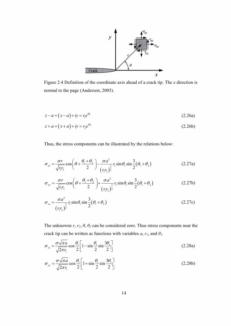
Figure 2.4 represents the multiple coordinate systems. Thus, auxiliary polar
coordinates can be defined by the relations according to Equation 2.26:
14
Figure 2.4 Definition of the coordinate axis ahead of a crack tip. The z direction is
normal to the page (Anderson, 2005).
1
1
iz a x a iy re
(2.26a)
2
2
iz a x a iy r e
(2.26b)
Thus, the stress components can be illustrated by the relations below:
2
1 21 1 1 23
1 2 21 2
3cos sin sin
2 2xx
r ar
r r r r
(2.27a)
2
1 21 1 1 23
1 2 21 2
3cos sin sin
2 2yy
r ar
r r r r
(2.27b)
2
1 1 1 23
21 2
3sin sin
2xx
ar
r r
(2.27c)
The unknowns r, r2, θ, θ2 can be considered zero. Thus stress components near the
crack tip can be written as functions with variables a, r1, and θ1.
1 1 1
1
3cos 1 sin sin
2 2 22xx
a
r
(2.28a)
1 1 1
1
3cos 1 sin sin
2 2 22yy
a
r
(2.28b)
15
1 1 1
1
3cos sin cos
2 2 22xy
a
r
(2.28c)
Since there is a stress singular zone around the crack tip in which state of stress is
adequately represented by a single parameter, K (the stress intensity factor SIF),
gives the strength of the singular field for small values of r1. Thus, when this stress
state becomes critical, a small crack grows and the material fails. This critical value
is called fracture toughness in some sources since it is a criterion for material
strength. The Mode-I SIF, KI, can be expressed as follows:
0
lim 2 ,0I yyr
K r x
(2.29)
Applying this definition to the ζyy stress for the central-crack problems from
Equation 2.28b, it can be found that;
IK a (2.30)
This is the SIF for mode-I type of loading for infinite sheet with a central-crack.
However, this formulation can be modified for various geometries by an additional
geometry function. It measures the strength of the singular field at the crack tip.
2.2.2 Energy Analysis Approach
As briefly described in the history of Fracture Mechanics, Griffith introduced the
energy approach for crack propagation in glass in 1915. It was later generalized by
Irwin who collected all available data to crack extension into a single term Gc, called
the strain energy release rate. Although the term rate generally refers to a derivative
with respect to time, here it does not. The term Gc is the rate of change in potential
energy with crack area. According to crack propagation in size, sufficient potential
16
energy must be available to overcome the surface energy of the material. The Griffith
Energy Theory for an increase in the crack area da, can be expressed as:
0STdWdE d
da da da
(2.31)
In Equation 2.31, ET describes the total energy, Π is the potential energy supplied by
internal strain energy and external force, and WS presents work required for creating
a new surface. There, the derivative of potential energy with respect to incremental
area of crack equals to the derivative of potential energy with respect to incremental
area of crack according to the theorem of minimum potential energy;
sdWd
da da
(2.32)
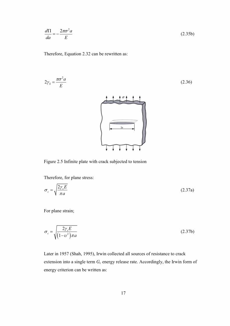
To show that WS is the change in the elastic surface energy due to formation of the
crack surface, consider an infinite plate of unit thickness that contains a crack length
2a subjected to uniform tensile stress, ζ, as shown in Figure 2.5. WS can be expressed
as follows:
4S SW a
(2.33)
where S is the surface energy of material. According to Inglis (Shah, 1995) , the
change in the strain, Π, can be written as;
2 2a
E
(2.34)
Thus;
4sS
dW
da
(2.35a)
17
22d a
da E
(2.35b)
Therefore, Equation 2.32 can be rewritten as:
2
2 S
a
E
(2.36)
Figure 2.5 Infinite plate with crack subjected to tension
Therefore, for plane stress:
2 sc
E
a
(2.37a)
For plane strain;
22
1
sc
E
a
(2.37b)
Later in 1957 (Shah, 1995), Irwin collected all sources of resistance to crack
extension into a single term Gc energy release rate. Accordingly, the Irwin form of
energy criterion can be written as:
18
For plane stress;
cc
EG
a
(2.38a)
For plane strain;
21
cc
EG
a
(2.38b)
where Gc is the strain energy release rate. The energy analysis approach proposes a
more convenient way for solving engineering problems.
2.2.3 Relationship between Stress Intensity Factor & Energy Release Rate
Since both the stress intensity factor and the strain energy release rate are criteria
which present a bulk material property, a relationship between K and G must exist.
Fortunately, these two material properties were developed as the extension of the
Griffith condition and applied only to the same geometry used, in an infinite sheet
under remote tension with a crack 2a long, as shown in Figure 2.5. Therefore, from
the theory developed in the previous chapter, at the instant of instability, the
following is obtained:
cK a (2.39)
Comparing Equations 2.37a and 2.38 for the same failure events in LEFM case
reveals that;
For plane stress;
19
2
c cK EG (2.40a)
For plane strain;
2
21
cc
EGK
(2.40b)
Although this generalization seems valid for an infinite sheet under remote tension,
this relationship between G and K for any geometry or crack configuration is
admissible for LEFM.
2.3 General Principles of Nonlinear Elastic Fracture Mechanics (NLEFM)
Approach
As introduced previously, energy principles can be used to describe critical energy
for crack propagation for nonlinear elastic, elastic-plastic and quasi-brittle material
properties. In the linear case, when the energy reaches a critical value, catastrophic
failure occurs. However, in nonlinear materials, a crack may steadily propagate up to
a critical length. NLEFM concept can be evaluated by using three main approaches
as follows;
Fracture Resistance Curve (R-Curve)
J-integral method
Crack Tip Opening Displacement
Fracture Resistance Curve can be used to characterize energy release rate to create a
unit crack area in the domain. Generally, it is a function of structural geometry and
material fracture properties. LEFM allows the stress to approach infinity at crack tip.
Since infinite stress cannot develop in real materials, a certain range of inelastic zone
must exist at the crack tip. This inelastic zone around a crack tip is termed fracture
20
process zone (FPZ). If the fracture process zone is small enough to ignore, function
may be regarded to depend only on the material geometry. Briefly, a structure with
an initial crack a0 and unit thickness should be considered. U is the total strain
energy produced by a load P. In this case, the energy release rate is a function of the
crack length a and the applied load P. It can be formulated as follows:
q
P
UG
a
(2.41)
Here Gq is a strain energy release rate in the nonlinear case. The crack propagation at
the crack tip requires consuming energy W. Therefore, the fracture resistance R can
be expressed as a function of crack extension as well as energy release rate. The
second-order derivative of potential energy can be considered to obtain sufficient
condition to identify the stability of crack propagation as follows;
qR Ga
(2.42)
2
2
qGR
a a a
(2.43)
Taking all these into account, several important observations can be made about
unstable fracture. The critical SIF is no longer a material property. As such, the
critical SIF depends on the geometry and the fracture process zone. Figure 2.6 shows
three different loads P1, P2 and P3 where P3>P2>P1. Although the curves
corresponding to P1 and P2 reach the critical point of the resistance curve, the crack
propagates even though the load decreases. Therefore, the relationship between R-
curve and the strain energy release rate can be archived as;
For stable crack growth 0qGR
a a
For stationary crack growth 0qGR
a a
For unstable crack growth 0qGR
a a
21
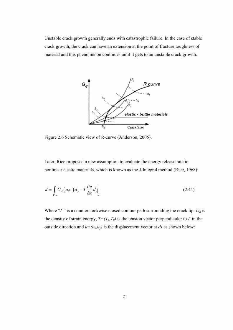
Unstable crack growth generally ends with catastrophic failure. In the case of stable
crack growth, the crack can have an extension at the point of fracture toughness of
material and this phenomenon continues until it gets to an unstable crack growth.
Figure 2.6 Schematic view of R-curve (Anderson, 2005).
Later, Rice proposed a new assumption to evaluate the energy release rate in
nonlinear elastic materials, which is known as the J-Integral method (Rice, 1968):
,d y s
uJ U a d T d
x
(2.44)
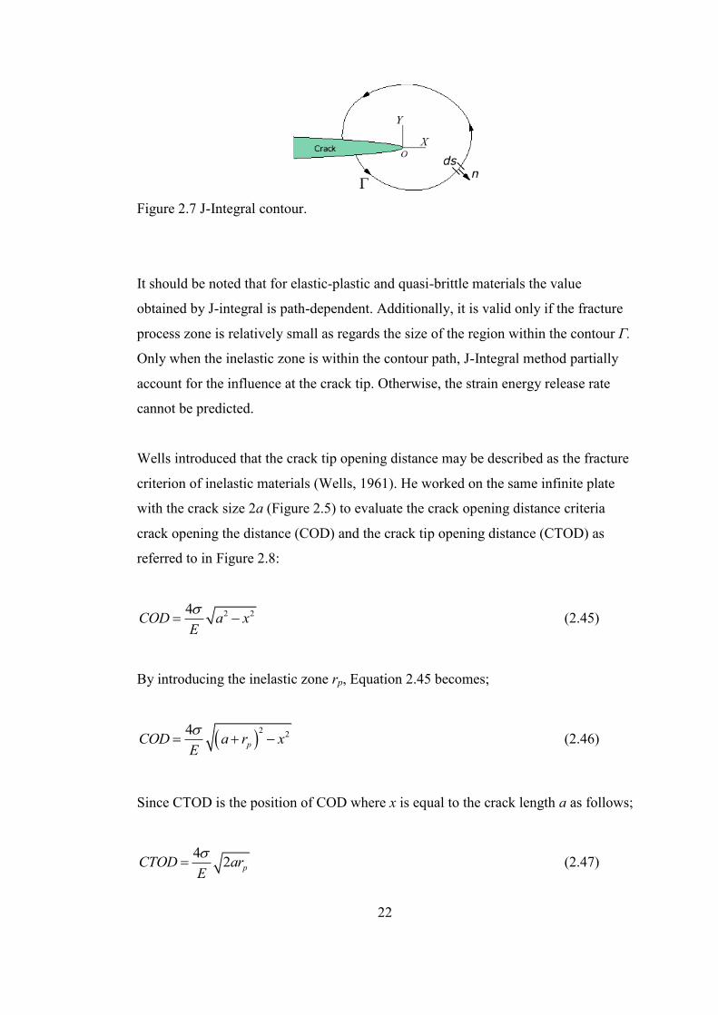
Where “Γ” is a counterclockwise closed contour path surrounding the crack tip. Ud is
the density of strain energy, T=(Tx,Ty) is the tension vector perpendicular to Γ in the
outside direction and u=(ux,uy) is the displacement vector at ds as shown below:
22
Figure 2.7 J-Integral contour.
It should be noted that for elastic-plastic and quasi-brittle materials the value
obtained by J-integral is path-dependent. Additionally, it is valid only if the fracture
process zone is relatively small as regards the size of the region within the contour Γ.
Only when the inelastic zone is within the contour path, J-Integral method partially
account for the influence at the crack tip. Otherwise, the strain energy release rate
cannot be predicted.
Wells introduced that the crack tip opening distance may be described as the fracture
criterion of inelastic materials (Wells, 1961). He worked on the same infinite plate
with the crack size 2a (Figure 2.5) to evaluate the crack opening distance criteria
crack opening the distance (COD) and the crack tip opening distance (CTOD) as
referred to in Figure 2.8:
2 24COD a x
E
(2.45)
By introducing the inelastic zone rp, Equation 2.45 becomes;
2
24pCOD a r x
E
(2.46)
Since CTOD is the position of COD where x is equal to the crack length a as follows;
42 pCTOD ar
E
(2.47)
23
According to Irwin (Irwin, 1960), the fracture process zone can be calculated by
using the yield strength
22
Ip
ys
Kr
(2.48)
By combining of equations 2.48 and 2.46, CTOD can be written as:
24 2 I
ys
KCTOD
E (2.49)
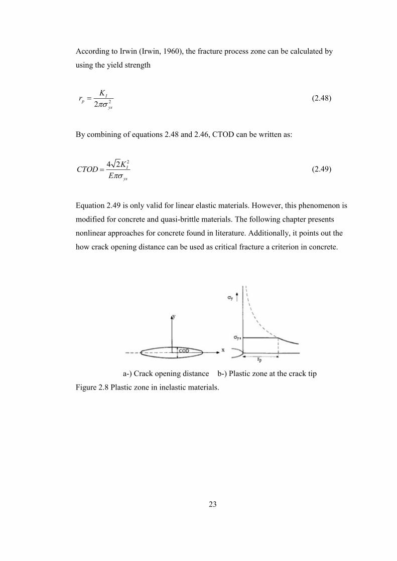
Equation 2.49 is only valid for linear elastic materials. However, this phenomenon is
modified for concrete and quasi-brittle materials. The following chapter presents
nonlinear approaches for concrete found in literature. Additionally, it points out the
how crack opening distance can be used as critical fracture a criterion in concrete.
a-) Crack opening distance b-) Plastic zone at the crack tip
Figure 2.8 Plastic zone in inelastic materials.
24
2.4 Fracture Mechanics of Concrete
2.4.1 Fictitious Crack Approach
Fracture behavior of concrete is mainly influenced by the fracture process zone as
that zone is quite large in comparison to crack size. In Figure 2.9, a crack model for
concrete is presented where an initial crack with length a0 and associated fracture
process zone Δa are described. In that figure, the concrete is assumed to have quasi-
brittle behavior. The cohesive pressure ζ(w) is a monotonic decreasing function of
crack separation displacement w. This model does not include the micro cracks ahead
of the crack tip. For the concrete fracture model, the energy release rate is prejudiced
by two different portions (Bažant, 2002),
1. The energy release rate consumed by creating two surfaces, GIc.
2. The energy rate to overcome the cohesive pressure, ζ(w), in separating the
surfaces Gζ.
Thus the energy release rate for a Mode-I quasi-brittle crack, Gq can be expressed as;
q IcG G G (2.50)
The value of GIc can be calculated by using LEFM and it is called critical energy
release rate. Since Gq is equal to the work done by cohesive pressure with unit
thickness, the expression may be evaluated as follows;
0 0 0 0 0
1 1( ) ( ) ( )
twa w a w
G w dxdw dx w dw w dwa a
(2.51)
where wt represents crack separation displacement at the initial crack tip. wc is the
critical crack separation. If crack separation is large enough, wt can be higher than wc.
25
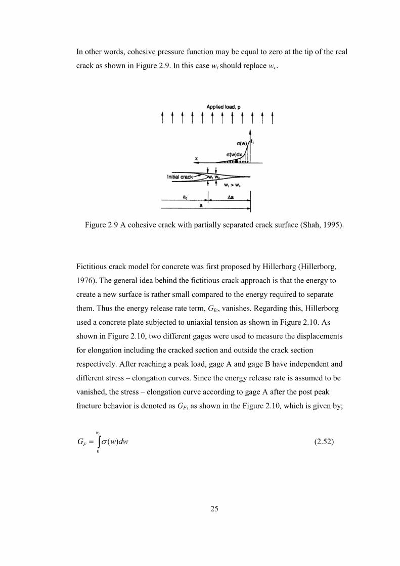
In other words, cohesive pressure function may be equal to zero at the tip of the real
crack as shown in Figure 2.9. In this case wt should replace wc.
Figure 2.9 A cohesive crack with partially separated crack surface (Shah, 1995).
Fictitious crack model for concrete was first proposed by Hillerborg (Hillerborg,
1976). The general idea behind the fictitious crack approach is that the energy to
create a new surface is rather small compared to the energy required to separate
them. Thus the energy release rate term, GIc, vanishes. Regarding this, Hillerborg
used a concrete plate subjected to uniaxial tension as shown in Figure 2.10. As
shown in Figure 2.10, two different gages were used to measure the displacements
for elongation including the cracked section and outside the crack section
respectively. After reaching a peak load, gage A and gage B have independent and
different stress – elongation curves. Since the energy release rate is assumed to be
vanished, the stress – elongation curve according to gage A after the post peak
fracture behavior is denoted as GF, as shown in the Figure 2.10, which is given by;
0
( )cw
FG w dw (2.52)
26
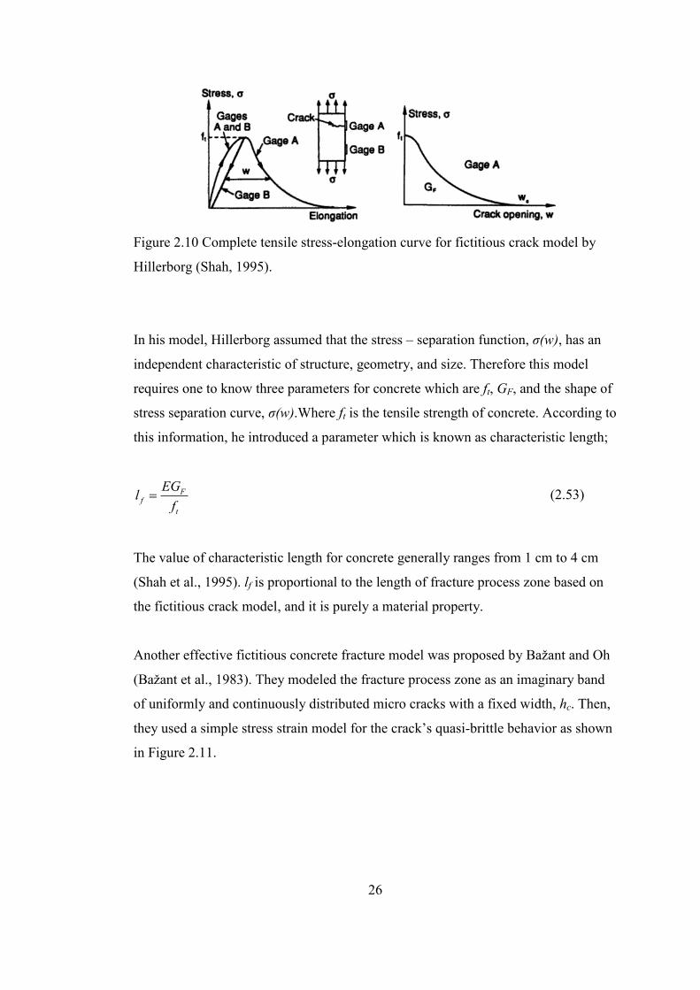
Figure 2.10 Complete tensile stress-elongation curve for fictitious crack model by
Hillerborg (Shah, 1995).
In his model, Hillerborg assumed that the stress – separation function, ζ(w), has an
independent characteristic of structure, geometry, and size. Therefore this model
requires one to know three parameters for concrete which are ft, GF, and the shape of
stress separation curve, ζ(w).Where ft is the tensile strength of concrete. According to
this information, he introduced a parameter which is known as characteristic length;
Ff
t
EGl
f (2.53)
The value of characteristic length for concrete generally ranges from 1 cm to 4 cm
(Shah et al., 1995). lf is proportional to the length of fracture process zone based on
the fictitious crack model, and it is purely a material property.
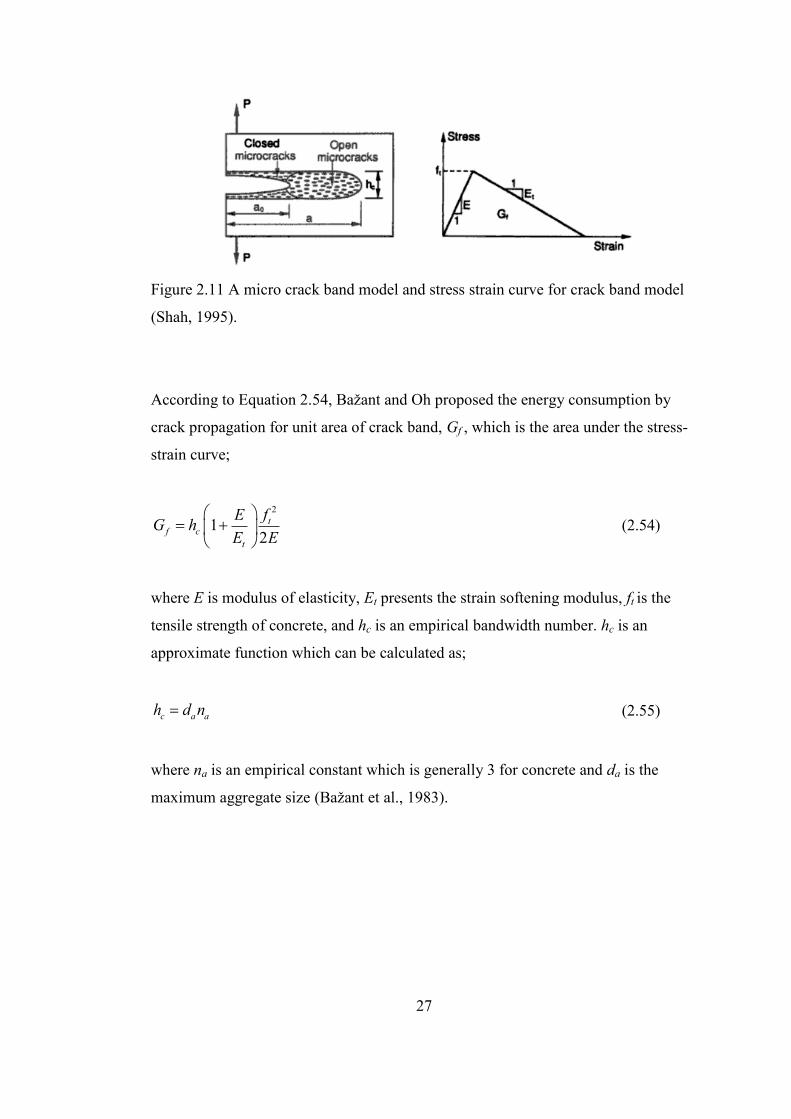
Another effective fictitious concrete fracture model was proposed by Bažant and Oh
(Bažant et al., 1983). They modeled the fracture process zone as an imaginary band
of uniformly and continuously distributed micro cracks with a fixed width, hc. Then,
they used a simple stress strain model for the crack’s quasi-brittle behavior as shown
in Figure 2.11.
27
Figure 2.11 A micro crack band model and stress strain curve for crack band model
(Shah, 1995).
According to Equation 2.54, Bažant and Oh proposed the energy consumption by
crack propagation for unit area of crack band, Gf , which is the area under the stress-
strain curve;
2
12
tf c
t
fEG h
E E
(2.54)
where E is modulus of elasticity, Et presents the strain softening modulus, ft is the
tensile strength of concrete, and hc is an empirical bandwidth number. hc is an
approximate function which can be calculated as;
c a ah d n (2.55)
where na is an empirical constant which is generally 3 for concrete and da is the
maximum aggregate size (Bažant et al., 1983).
28
2.4.2 Effective-Elastic Crack Approach
Contrary to fictitious crack models, in effective - elastic crack models, concrete
fracture criterion is modeled by an assumption that the stress - separation function,
ζ(w), is neglected. Therefore, fracture process zone effect must be included in the
calculation. Hence, this model is governed by LEFM behavior. As a result, the
energy release rate for Mode-I type loading may be calculated as;
q IcG G (2.56)
where Gq is a function of structural size and applied load as well as crack length and
orientation. Since the crack length will increase by increment of the loading for the
case of stable crack propagation, an additional equation should be provided to
calculate the effective crack length. Unfortunately, since this effective crack length
depends on geometry and size, it may not be used as an independent and unique
fracture criterion. Thus, another fracture quantity should be introduced. Therefore,
the general approach of effective-elastic crack approach uses more than one criterion.
Jenq and Shah’s approach which is known as the “Two parameter fracture model”
can be introduced as one of the most popular concrete effective elastic fracture
models (Jenq and Shah, 1985). In their two-parameter fracture model, in order to
separate the elastic and plastic responses of a given specimen, Jenq and Shah loaded
the specimen up to a maximum stress and then they unloaded and reloaded it as
shown in Figure 2.12.
29
Figure 2.12 Elastic and plastic fracture responses and loading and unloading
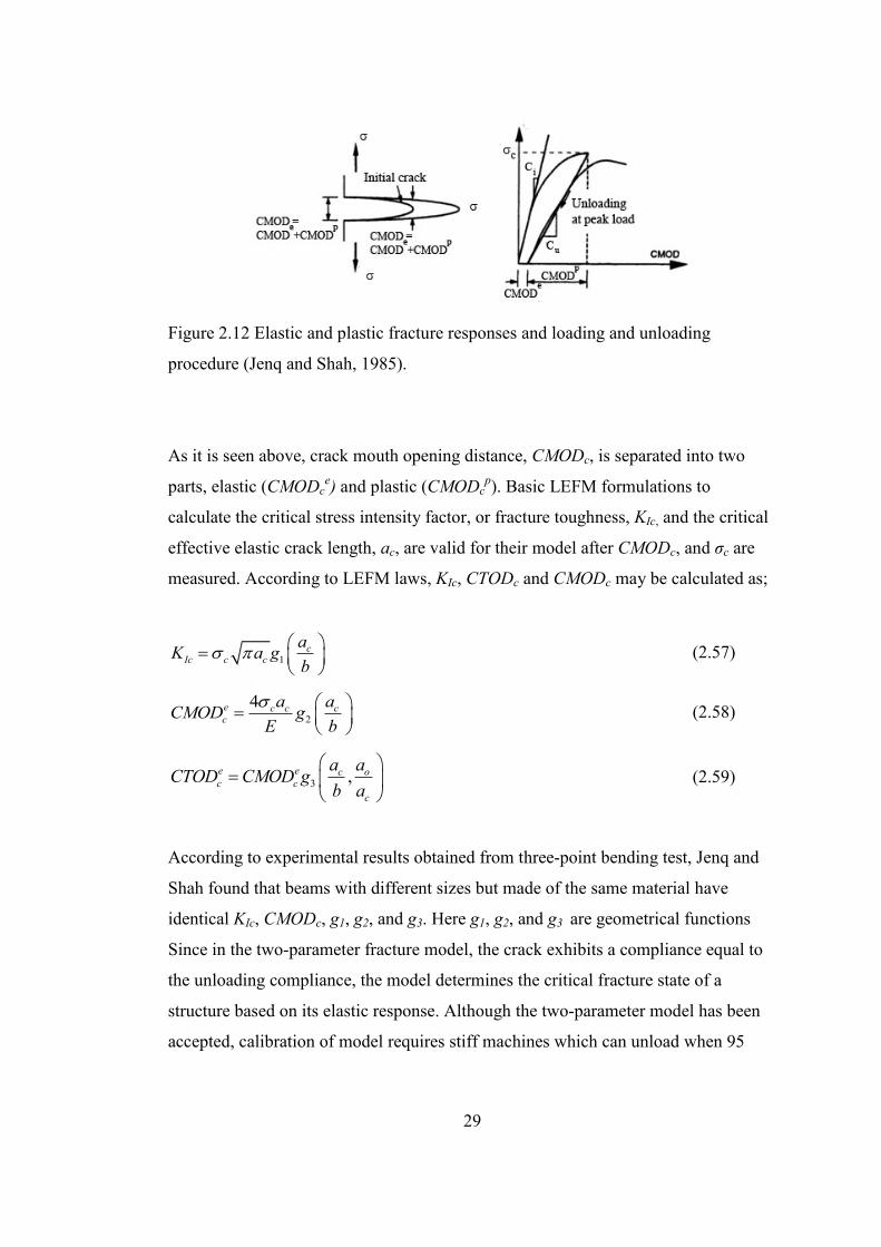
procedure (Jenq and Shah, 1985).
As it is seen above, crack mouth opening distance, CMODc, is separated into two
parts, elastic (CMODce) and plastic (CMODc
p). Basic LEFM formulations to
calculate the critical stress intensity factor, or fracture toughness, KIc, and the critical
effective elastic crack length, ac, are valid for their model after CMODc, and ζc are
measured. According to LEFM laws, KIc, CTODc and CMODc may be calculated as;
1c
Ic c c
aK a g
b
(2.57)
2
4e c c cc
a aCMOD g
E b
(2.58)
3 ,e e c oc c
c
a aCTOD CMOD g
b a
(2.59)
According to experimental results obtained from three-point bending test, Jenq and
Shah found that beams with different sizes but made of the same material have
identical KIc, CMODc, g1, g2, and g3. Here g1, g2, and g3 are geometrical functions
Since in the two-parameter fracture model, the crack exhibits a compliance equal to
the unloading compliance, the model determines the critical fracture state of a
structure based on its elastic response. Although the two-parameter model has been
accepted, calibration of model requires stiff machines which can unload when 95
30
percent of ultimate load is reached followed by reloading. They also introduced a
parameter which is known as a material length, Q, expressed as follows;
2
c
Ic
E CMODQ
K
(2.60)
Higher values of Q mean a more ductile material. According to their experimental
observations, they proposed that KIc, CTOD, and E can be calculated by using the
compressive strength of concrete, fc as follows;
0.75
0.06Ic cK f (2.61)
0.13
0.00602c cCTOD f (2.62)
4785 cE f (2.63)
where KIc is in MPa m and CTODc is millimeters, and E and fc are in MPa .
Another reason to use the two parameter model to the predict fracture process of
concrete is that all materials in nature have flaws, and when concrete is loaded, these
flaws may propagate and directly be linked with the crack tip. Although in ductile
materials, a single parameter can be used to predict fracture toughness, brittle
materials, especially concrete, require more than one parameter because of the size of
the wake process zone. Therefore, CTODc is used together with KIc to determine the
critical crack propagation for quasi-brittle materials.
In 1990, Bažant and Kazemi introduced a simulation of fracture of quasi-brittle
materials by a modified version of Bažant and Ohs’ crack band model by means of
effective-elastic crack approach (Bažant and Kazemi, 1990). They used a series of
three-point bending test specimens with the constant ratio of initial crack length (ao)
to the dimension of depth (D). For these geometrically similar structures with ao,
they found that the nominal stress failure may be described as follows:
31
n cc
c P
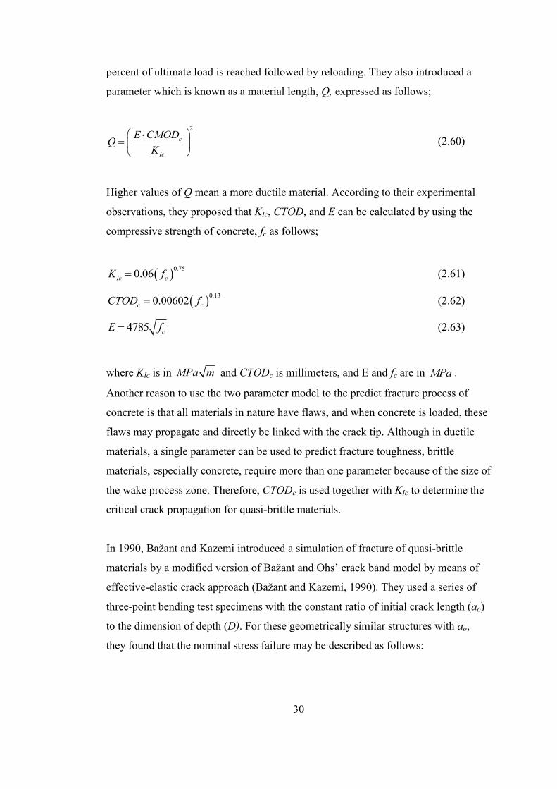
tD (2.64)
where Pc is the peak load, t is the thickness of specimen, D represents the depth, and
S is the span for a three-point bending test specimen as shown in Figure 2.13;
Figure 2.13 Series of geometrically similar three-point bending test structures.
cn is a constant which can be calculated in linear case as follows ;
1.5n
Sc
D (2.65)
Bažant and Kazemi used the expression above for LEFM formulations. According to
their model, the critical energy release rate for a certain size of concrete structure can
be written as:
2 2 22
1 2
Ic c c c c cIc
K a a P aG g g
E E D Et D D
(2.66)
32
where again ac = ao + Δa is the critical crack length and cagD
is a geometric
function which is given by;
22
1c n c ca c a a
g gD D D
(2.67)
Bažant, in his previous studies, worked on the failure stress of the geometrically
similar structures. He, then, demonstrated that up to 1
20o
D
D nominal stresses can
be expressed as follows:
1
tNc
o
Bf
D
D
(2.68)
where B is a constant based on the effective elastic crack approach and Do is another
constant which is called characteristic size. Bažant and Kazemi proposed using a
critical energy release rate and critical crack extension for an infinitely large
structure in order to eliminate the length of the crack extension. Therefore, two
different parameters are defined in their article;
2 2 2
2 2lim lim Nc c t o o
f IcD D
n n
D a B f D aG G g g
Ec D Ec D
(2.69)
As discussed previously, another parameter is necessary to obtain a fracture
mechanism of concrete. The authors introduced the second parameter as critical
crack extension, cf, for an infinite large specimen. In order to obtain the critical crack
extension, they expanded the geometric function fa
gD
into a Taylor series only up
to first order terms as follows;
33
limf cD
c a
(2.70)
f f fo o o o oa a ca a a a a
g g g g gD D D D D D D D
(2.71)
where;
f o fa a c (2.72)
As a result, the critical crack extension for large specimen can be expressed as;
o
f o
o
agD
c Da
gD
(2.73)
In 1991, Planas and Elices compared the fictitious crack model, the size effect
model, and the two parameter fracture model. For that purpose, a series of similar
three-point bending beam structures were tested. The values of Gf, GIcs were obtained
from the size effect model and the two-parameter model for comparisons. As a result
of those experiments, they obtained Gf=0.52 GF and GIcs=0.48 GF as D approaches
infinity. Therefore Gf and GIcs are comparable. It is also noted that GIc
s or Gf is the
rate of strain energy required to extend a crack. On the other hand, GF is the energy
per unit area to completely to separate a fracturing material. Therefore, the value of
GF is approximately twice as great as the values of Gf and GIcs. It is also reported that
the peak load prediction for an infinitely large structure by the size effect model and
the two parameter fracture model are 28.1 and 30.8 % lower than the one predicted
by the fictitious crack model (Planas and Elices, 1992).
34
2.5 Finite Element Analysis of Fracture Mechanics Properties
2.5.1 Finite Element Modeling of Singularities
In finite element modeling of cracks and stress singular parts of structure, it is
necessary to have not only very refined mesh but also special elements at the crack
tip. Three main approaches are developed to improve the accuracy of FEM and to
obtain more realistic solutions:
i. Enriched finite elements
ii. Singular finite elements
iii. Hp-finite elements
In general, in finite element analysis, finer meshes usually yield solutions that are
closer to the exact solution. However, it is not always the case for the fracture
mechanics analysis. As mentioned in the previous sections, there is an inverse square
root singularity at the crack tip. Singular finite elements are the most popular
solutions to solve this kind of singularities. For one layered domain, Barsom in 1976
demonstrated that mathematical exact solution of square root singularity can be
obtained by replacing the mid-side nodes to the quarter point position. The concept
of the quarter-point singular element was generalized by Staab in 1983. Therefore,
by varying the placement of the mid-side node, it is possible to model any
singularity.
In order to understand the concept of quarter point singular elements, the formulation
of shape function of isoparametric singular finite elements can be explained for one-
dimensional elements as shown in Figure 2.14. The equation is given as follows:
35
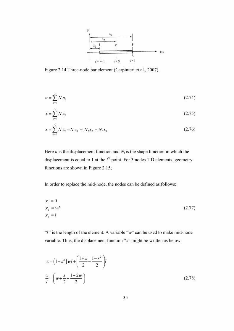
Figure 2.14 Three-node bar element (Carpinteri et al., 2007).
3
1
i i
i
u N u
(2.74)
3
1
i i
i
x N x
(2.75)
3
1 1 2 2 3 3
1
i i
i
x N x N x N x N x
(2.76)
Here u is the displacement function and Ni is the shape function in which the
displacement is equal to 1 at the ith
point. For 3 nodes 1-D elements, geometry
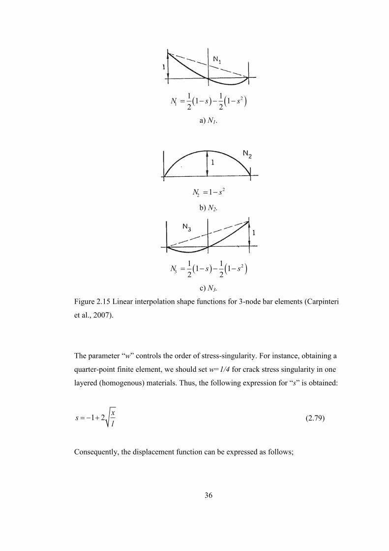
functions are shown in Figure 2.15;
In order to replace the mid-node, the nodes can be defined as follows;
1
2
3
0x
wlx
lx
(2.77)
“l” is the length of the element. A variable “w” can be used to make mid-node
variable. Thus, the displacement function “x” might be written as below;
2
2 1 11
2 2
s sx s wl l
1 2
2 2
x s ww
l
(2.78)
36
21
1 11 1
2 2N s s
a) N1.
2
21N s
b) N2.
23
1 11 1
2 2N s s
c) N3.
Figure 2.15 Linear interpolation shape functions for 3-node bar elements (Carpinteri
et al., 2007).
The parameter “w” controls the order of stress-singularity. For instance, obtaining a
quarter-point finite element, we should set w=1/4 for crack stress singularity in one
layered (homogenous) materials. Thus, the following expression for “s” is obtained:
1 2x
sl
(2.79)
Consequently, the displacement function can be expressed as follows;
37
3
1 2 3
1
1 3 2 4 4 2i i
i
x x x x x xu N u u u u
l l l l l l
(2.80)
As a result, the stress components along x-coordinate tend to go to infinity as x goes
to 0, with a power of singularity equal to negative square root;
0 0 0
1lim lim limxx x x
u
x x
(2.81)
0 0 0 0
1lim lim lim limx xx x x x
uE E
x x
(2.82)
Since stress goes to infinity at the crack tip, FEM model and the exact mathematical
model of domain can have a better match. Therefore, the calculation of stress
singularity at the crack tip is able to have more realistic results according to mesh
size and stress singular elements at the crack tip. In the FE computer package
ANSYS©
, there is a special meshing tool which defines a concentration key point
about which area mesh will be skewed. During skewing, a user can specify the
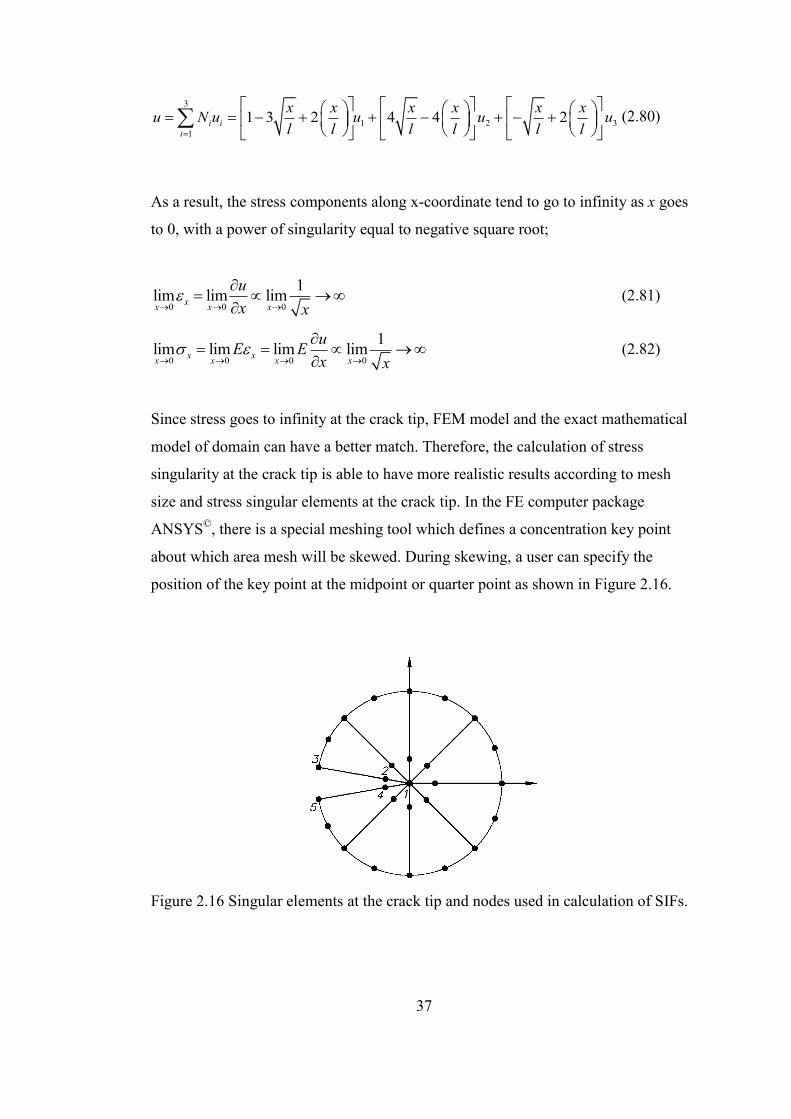
position of the key point at the midpoint or quarter point as shown in Figure 2.16.
Figure 2.16 Singular elements at the crack tip and nodes used in calculation of SIFs.

38
It is recommended that for the best accuracy, length of each singular element at the
crack tip should be less than eight times of crack length, and angle at the crack tip
should be between 30o and 40
o (Cook et al., 2001)
2.5.2 Calculation of Stress Intensity Factor Using Finite Element Method
In the previous sections, it is mentioned that SIF is calculated to obtain the stress
singularity value at the crack tip for different modes of crack. As aforementioned, in
this study the problem of a crack in a concrete under LEFM condition is presented.
In FEM, there are three main methods presented in the literature to estimate SIF as
follows (ACI, 2009);
Displacement Correlation Technique (DCT)
Stress Correlation Technique (SCT)
Energy release rate methods
J-Integral Method
Potential energy derivative approaches
In this study, to obtain force “P” versus mid span displacement “δ” curve of a beam
in bending crack propagation analysis is performed by DCT. Moreover, to see effect
of meshing and elements types, DCT results are compared with handbook
calculations.
The displacement correlation technique has been a widely used technique to evaluate
the stress intensity factor since FEM and computer applications became an important
part of analyses. Kim and Paulino evaluated Mode-I and mixed-mode two-
dimensional problems (Kim and Paulino, 2002). In this thesis, displacement
correlation technique is utilized by application of linear elastic fracture mechanics for
concrete. In brief, a three-dimensional crack front under Mode-I loading as shown in
Figure 2.19 is considered (ACI, 2009).
39
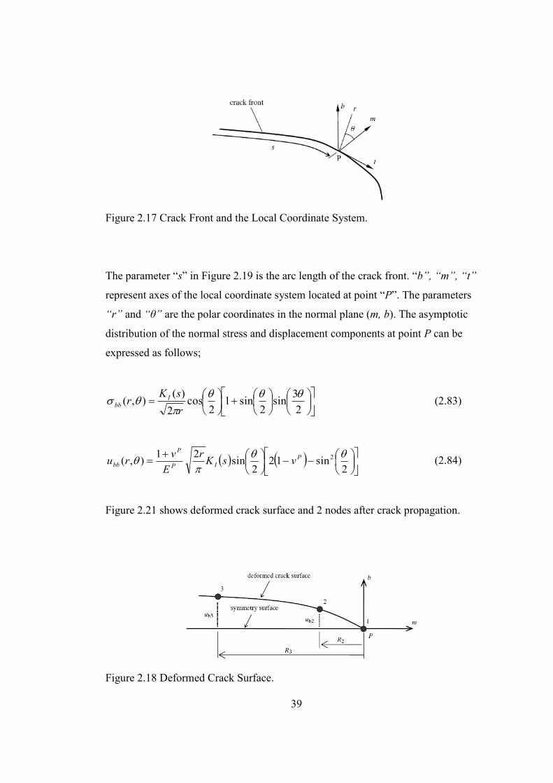
Figure 2.17 Crack Front and the Local Coordinate System.
The parameter “s” in Figure 2.19 is the arc length of the crack front. “b”, “m”, “t”
represent axes of the local coordinate system located at point “P”. The parameters
“r” and “θ” are the polar coordinates in the normal plane (m, b). The asymptotic
distribution of the normal stress and displacement components at point P can be
expressed as follows;
2
3sin
2sin1
2cos
2
)(),(
r
sKr I
bb (2.83)
2sin12
2sin
21),( 2
P
IP
P
bb vsKr
E
vru (2.84)
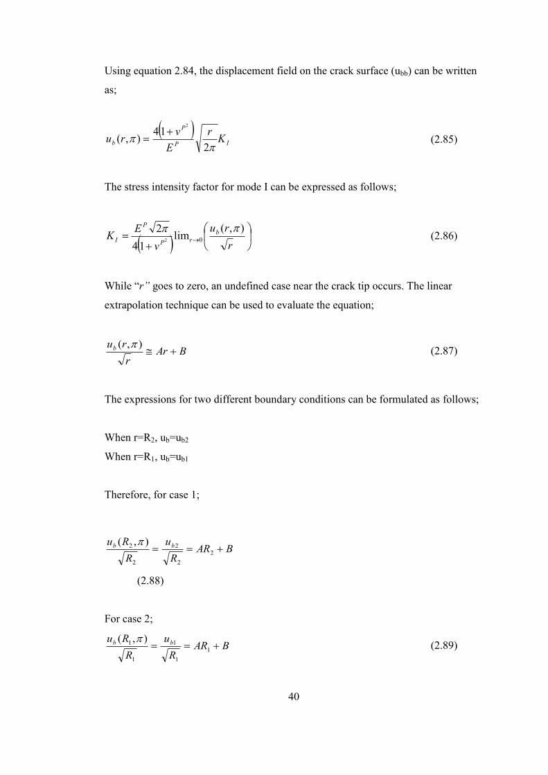
Figure 2.21 shows deformed crack surface and 2 nodes after crack propagation.
Figure 2.18 Deformed Crack Surface.
40
Using equation 2.84, the displacement field on the crack surface (ubb) can be written
as;
IP
P
b Kr
E
vru
2
14),(
2
(2.85)
The stress intensity factor for mode I can be expressed as follows;
r
ru
v
EK b
rP
P
I
),(lim
14
202
(2.86)
While “r” goes to zero, an undefined case near the crack tip occurs. The linear
extrapolation technique can be used to evaluate the equation;
BArr
rub ),(
(2.87)
The expressions for two different boundary conditions can be formulated as follows;
When r=R2, ub=ub2
When r=R1, ub=ub1
Therefore, for case 1;
BARR
u
R
Ru bb 2
2
2
2
2 ),(
(2.88)
For case 2;
BARR
u
R
Ru bb 1
1
1
1
1 ),( (2.89)
41
Using Equations 2.88 and 2.89, new equations can be evaluated as unknowns “A”,
and “B”;
2332
2332
RRRR
uRuRA
bb
(2.90)
2332
2
2/3
23
2/3
3
RRRR
uRuRB bb
(2.91)
If “r” value is very small, “A” value vanishes at the crack tip. Therefore, the
expression r
rub ),( will be equal to “B” as “r” equals to zero.
B
v
EK
P
P
I 2
14
2
(2.92)
Using equations 2.91 and 2.92, the stress intensity factor KI can now be expressed as
below.
2332
2
2/3
23
2/3
3
2
14
2
RRRR
uRuR
v
EK bb
P
P
I
(2.93)
As presented above, after the finite element calculation, by using displacements and
distances at crack tip of the two nodes on the crack surface, it is easy to find SIF.
2.5.3 The Main Feature and Hypothesis of Finite Element Analysis of Fracture
in Concrete
It became apparent that concrete structures usually do not behave in a way consistent
with the assumption of classical continuum mechanics (Bažant, 1976). Fortunately,
in the work done so far, it has been mentioned that two approaches may be used to
estimate concrete fracture behavior by FEM.
42
The first approach is known as the smeared crack model. The smeared crack
approach was first introduced by Rashid. This approach is based on the concept of
replacing a crack by a continuous medium with altered properties (Rashid, 1968).
The earliest approach is to change the element stiffness to zero, once the stress is
calculated to exceed the tensile strength capacity of the material. Over the years,
numerical applications of smeared crack model have been challenged by the strain
localization problem.
The second approach, discrete crack model is an elder, however still widely used
finite element model to evaluate crack propagation and fracture damage of structure
for concrete and quasi-brittle materials. There are three problems to be solved:
determining the location and initiation direction of the initial crack, determining how
the crack extends, and determining the direction of crack extension. The first issue
can be solved on the basis of maximum tensile stress. Crack extension may be
determined for LEFM problems by considering the SIF associated with stress state at
the crack tip. When SIF exceeds the fracture toughness, the crack propagates.
Alternatively, energy release rate can be used. After this process, the crack length
should be increased, then remeshing will be performed to incorporate the new crack
direction and the same process must be executed up to structure failure occurs or the
model cannot take any more load. Remeshing is the main disadvantage of the
discrete crack model.
Nowadays, the cohesive crack model is widely used for the analysis of propagating
cracks in concrete and other quasi brittle materials. In Figure 2.19, a schematic
description of crack propagation for concrete is presented. Two different zones can
be distinguished in this figure. The left is the stress free zone, where crack faces are
completely stress-free. The faces are completely disconnected. The Second zone on
the right is the damage zone also called the fracture process zone. As it can be seen
in Figure 2.19, there are micro cracks and flaws in this zone. This case is totally
different from LEFM. However, as explained earlier, there are some ways to convert
the LEFM approach into the cohesive approach.

43
Figure 2.19 Cohesive crack model and damage zone in concrete (Carpinteri et al.,
2007).
From 1984 to 1989 Carpinteri tried to figure out how Hillerborg’s fictitious model
can be used for finite element analysis. He proposed that nonlinear behavior of
concrete at the damage zone can be subjected to the nodes after increasing crack
length as shown in the figure below;
Figure 2.20 Finite element view of discrete crack model (Carpinteri et al., 2007).
In finite element calculation, formulation of cohesive traction forces can be
calculated as follows;

44
Figure 2.21 Finite element analysis of three-point bending beam (Carpinteri et al.,
2007).
If the damage zone is absent;
w K F C P (2.94)
where, w is the vector of the crack opening distance, [K] is the matrix of the
coefficients of influence when subjected to force of a unit. {F} is vector of the nodal
cohesive traction force; {C} is vector of the coefficients of influence when domain is
subjected to the force P.
If the damage zone is present between nodes j and n, cohesive forces can be
calculated as follows;
0 1,....., ( 1)
,.....,
0
i
t
i
F for i j
F F w for i j n
w for i n
(2.95)
Consequently, cohesive traction force in the quasi-brittle material is integrated into
the model as shown in the fictitious crack model. In this case, concrete fracture
criteria may be crack tip stresses. When it is equal to ultimate tensile stress of the
material, crack propagation occurs. Discrete crack model laws are valid for this
model, therefore, the crack length increases until the failure of model is observed.
45
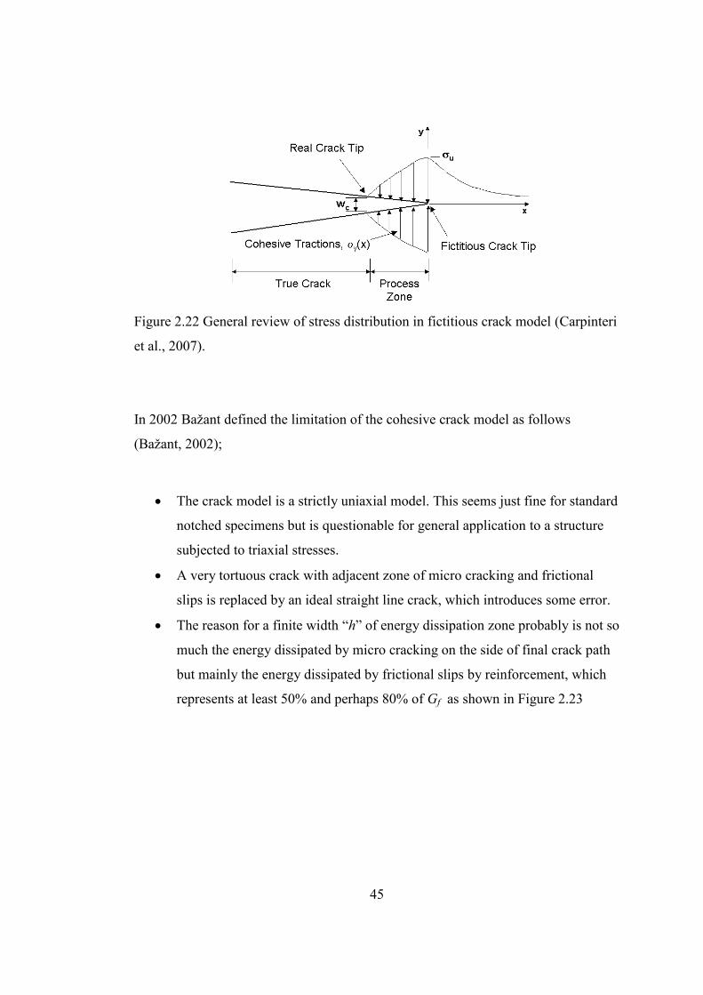
Figure 2.22 General review of stress distribution in fictitious crack model (Carpinteri
et al., 2007).
In 2002 Bažant defined the limitation of the cohesive crack model as follows
(Bažant, 2002);
The crack model is a strictly uniaxial model. This seems just fine for standard
notched specimens but is questionable for general application to a structure
subjected to triaxial stresses.
A very tortuous crack with adjacent zone of micro cracking and frictional
slips is replaced by an ideal straight line crack, which introduces some error.
The reason for a finite width “h” of energy dissipation zone probably is not so
much the energy dissipated by micro cracking on the side of final crack path
but mainly the energy dissipated by frictional slips by reinforcement, which
represents at least 50% and perhaps 80% of Gf as shown in Figure 2.23
46
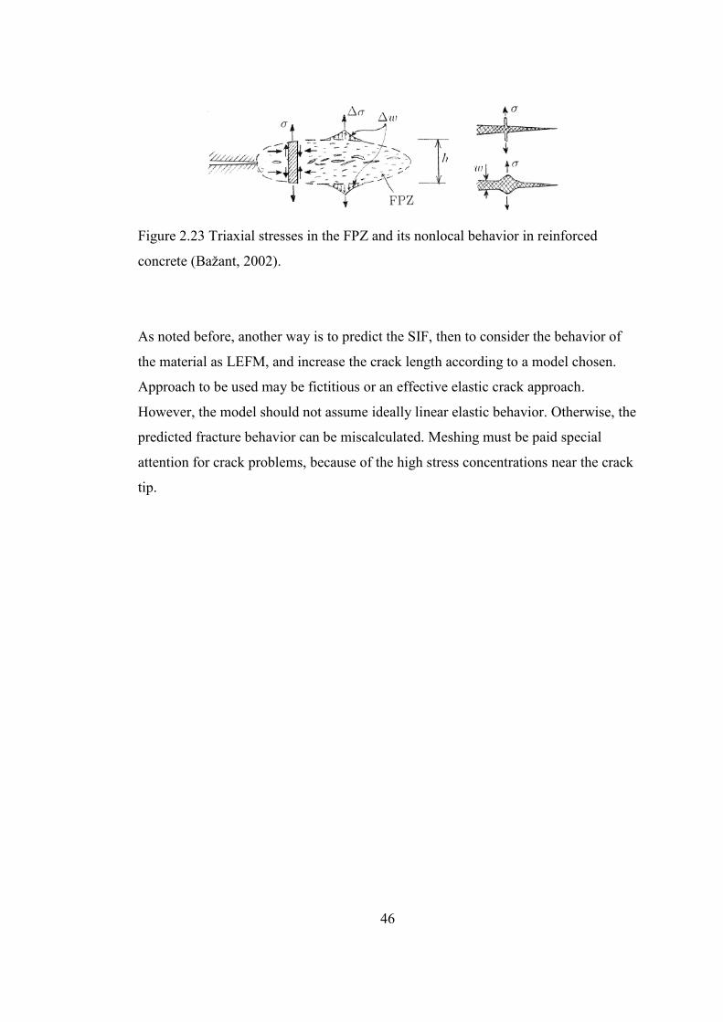
Figure 2.23 Triaxial stresses in the FPZ and its nonlocal behavior in reinforced
concrete (Bažant, 2002).
As noted before, another way is to predict the SIF, then to consider the behavior of
the material as LEFM, and increase the crack length according to a model chosen.
Approach to be used may be fictitious or an effective elastic crack approach.
However, the model should not assume ideally linear elastic behavior. Otherwise, the
predicted fracture behavior can be miscalculated. Meshing must be paid special
attention for crack problems, because of the high stress concentrations near the crack
tip.
47
CHAPTER 3
INTRINSIC PARAMETERS OF FINITE ELEMENT ANALYSIS OF
FRACTURE
3
In this chapter, the first objective of the thesis is investigated. For this purpose,
earlier studies for finite element size in the finite element solutions of fracture of
concrete are mentioned. Then the three-point bending test specimen in ASTM
standards is compared with solution by FEM with various mesh sizes and element
types. Thus, the accuracy of the finite element solutions is presented.
3.1 The Issue of Stability of Crack Propagation
The role of finite element size in the concrete fracture analysis was first presented by
Carpinteri (Carpinteri et al., 2007). According to the work carried out by him and his
coworkers, the mesh refinement was taken into consideration with respect to
brittleness number. The brittleness number is related to not only material but also the
geometry and size of structure. The greater value of the brittleness number, the more
is the brittle characterized of the structure. In this study, brittleness number (or
Carpinteri number) is described as follows:
f
u
GSE
h (3.1)
With this purpose, they used the cohesive crack model with 3 different mesh
refinements which have 20, 40 and 80 elements at the fracture face, respectively, as
shown in Figure 3.1. Providing the relationship between mesh refinement and
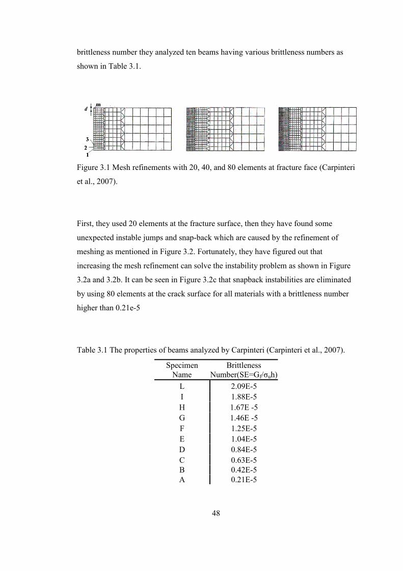
48
brittleness number they analyzed ten beams having various brittleness numbers as
shown in Table 3.1.
Figure 3.1 Mesh refinements with 20, 40, and 80 elements at fracture face (Carpinteri
et al., 2007).
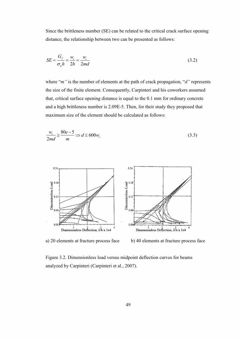
First, they used 20 elements at the fracture surface, then they have found some
unexpected instable jumps and snap-back which are caused by the refinement of
meshing as mentioned in Figure 3.2. Fortunately, they have figured out that
increasing the mesh refinement can solve the instability problem as shown in Figure
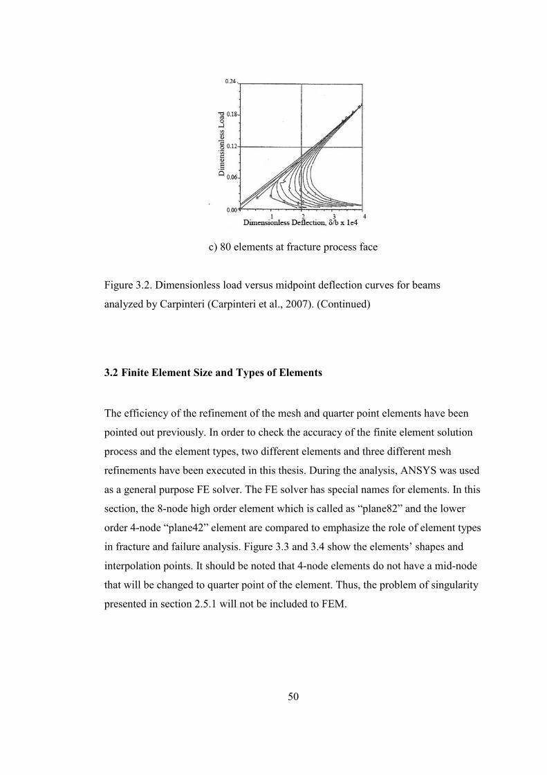
3.2a and 3.2b. It can be seen in Figure 3.2c that snapback instabilities are eliminated
by using 80 elements at the crack surface for all materials with a brittleness number
higher than 0.21e-5
Table 3.1 The properties of beams analyzed by Carpinteri (Carpinteri et al., 2007).
Specimen
Name
Brittleness
Number(SE=Gf/σuh)
L 2.09E-5
I 1.88E-5
H 1.67E -5
G 1.46E -5
F 1.25E-5
E 1.04E-5
D 0.84E-5
C 0.63E-5
B 0.42E-5
A 0.21E-5
49
Since the brittleness number (SE) can be related to the critical crack surface opening
distance, the relationship between two can be presented as follows:
2 2
f c c
u
G w wSE
h h md (3.2)
where “m” is the number of elements at the path of crack propagation, “d” represents
the size of the finite element. Consequently, Carpinteri and his coworkers assumed
that, critical surface opening distance is equal to the 0.1 mm for ordinary concrete
and a high brittleness number is 2.09E-5. Then, for their study they proposed that
maximum size of the element should be calculated as follows:
80 5600
2
cc
w ed w
md m
(3.3)
a) 20 elements at fracture process face b) 40 elements at fracture process face
Figure 3.2. Dimensionless load versus midpoint deflection curves for beams
analyzed by Carpinteri (Carpinteri et al., 2007).
50
c) 80 elements at fracture process face
Figure 3.2. Dimensionless load versus midpoint deflection curves for beams
analyzed by Carpinteri (Carpinteri et al., 2007). (Continued)
3.2 Finite Element Size and Types of Elements
The efficiency of the refinement of the mesh and quarter point elements have been
pointed out previously. In order to check the accuracy of the finite element solution
process and the element types, two different elements and three different mesh
refinements have been executed in this thesis. During the analysis, ANSYS was used
as a general purpose FE solver. The FE solver has special names for elements. In this
section, the 8-node high order element which is called as “plane82” and the lower
order 4-node “plane42” element are compared to emphasize the role of element types
in fracture and failure analysis. Figure 3.3 and 3.4 show the elements’ shapes and
interpolation points. It should be noted that 4-node elements do not have a mid-node
that will be changed to quarter point of the element. Thus, the problem of singularity
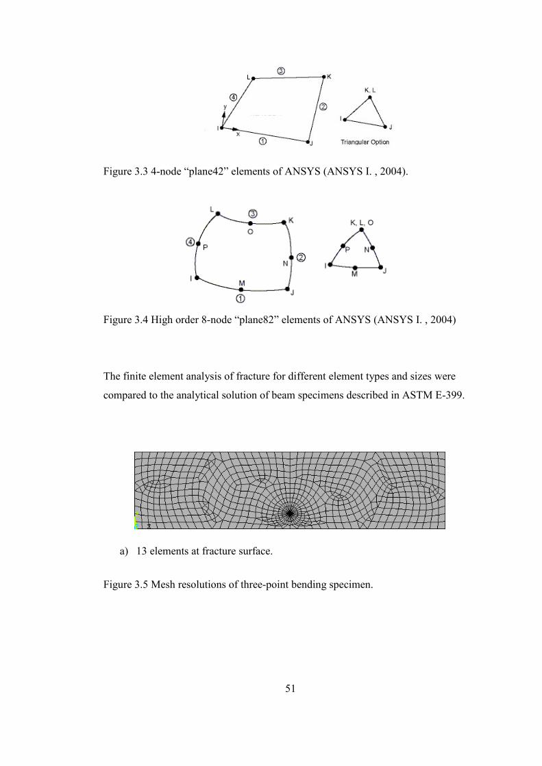
presented in section 2.5.1 will not be included to FEM.
51
Figure 3.3 4-node “plane42” elements of ANSYS (ANSYS I. , 2004).
Figure 3.4 High order 8-node “plane82” elements of ANSYS (ANSYS I. , 2004)
The finite element analysis of fracture for different element types and sizes were
compared to the analytical solution of beam specimens described in ASTM E-399.
a) 13 elements at fracture surface.
Figure 3.5 Mesh resolutions of three-point bending specimen.
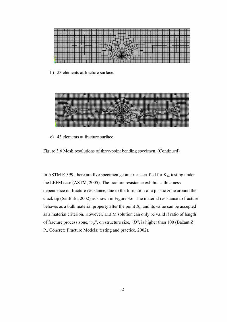
52
b) 23 elements at fracture surface.
c) 43 elements at fracture surface.
Figure 3.6 Mesh resolutions of three-point bending specimen. (Continued)
In ASTM E-399, there are five specimen geometries certified for KIC testing under
the LEFM case (ASTM, 2005). The fracture resistance exhibits a thickness
dependence on fracture resistance, due to the formation of a plastic zone around the
crack tip (Sanforld, 2002) as shown in Figure 3.6. The material resistance to fracture
behaves as a bulk material property after the point Bc, and its value can be accepted
as a material criterion. However, LEFM solution can only be valid if ratio of length
of fracture process zone, “rp”, on structure size, ”D”, is higher than 100 (Bažant Z.
P., Concrete Fracture Models: testing and practice, 2002).
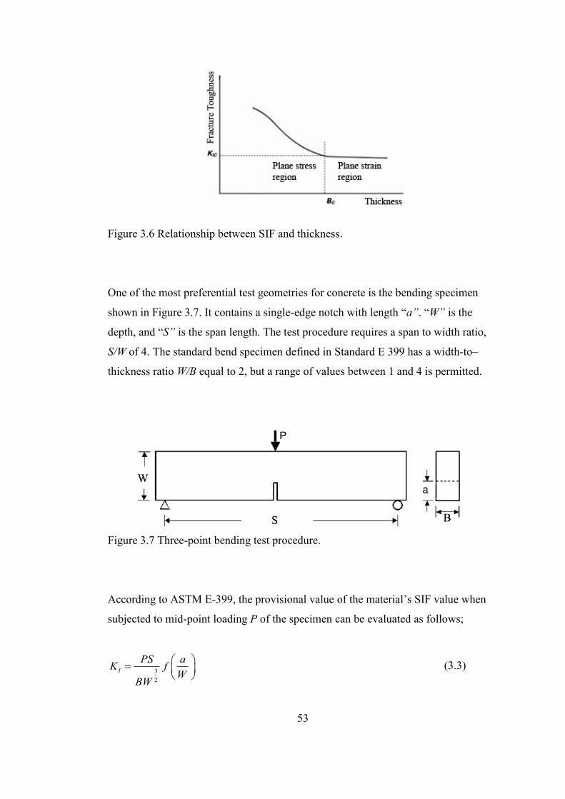
53
Figure 3.6 Relationship between SIF and thickness.
One of the most preferential test geometries for concrete is the bending specimen
shown in Figure 3.7. It contains a single-edge notch with length “a”. “W” is the
depth, and “S” is the span length. The test procedure requires a span to width ratio,
S/W of 4. The standard bend specimen defined in Standard E 399 has a width-to–
thickness ratio W/B equal to 2, but a range of values between 1 and 4 is permitted.
Figure 3.7 Three-point bending test procedure.
According to ASTM E-399, the provisional value of the material’s SIF value when
subjected to mid-point loading P of the specimen can be evaluated as follows;
3
2
I
PS aK f
WBW
(3.3)
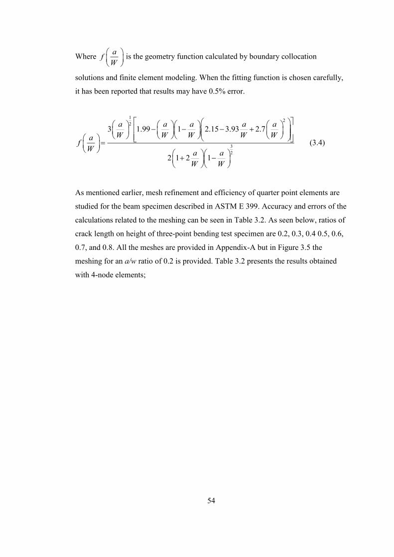
54
Where a
fW
is the geometry function calculated by boundary collocation
solutions and finite element modeling. When the fitting function is chosen carefully,
it has been reported that results may have 0.5% error.
12
2
3
2
3 1.99 1 2.15 3.93 2.7
2 1 2 1
a a a a a
W W W W WafW
a a
W W
(3.4)
As mentioned earlier, mesh refinement and efficiency of quarter point elements are
studied for the beam specimen described in ASTM E 399. Accuracy and errors of the
calculations related to the meshing can be seen in Table 3.2. As seen below, ratios of
crack length on height of three-point bending test specimen are 0.2, 0.3, 0.4 0.5, 0.6,
0.7, and 0.8. All the meshes are provided in Appendix-A but in Figure 3.5 the
meshing for an a/w ratio of 0.2 is provided. Table 3.2 presents the results obtained
with 4-node elements;
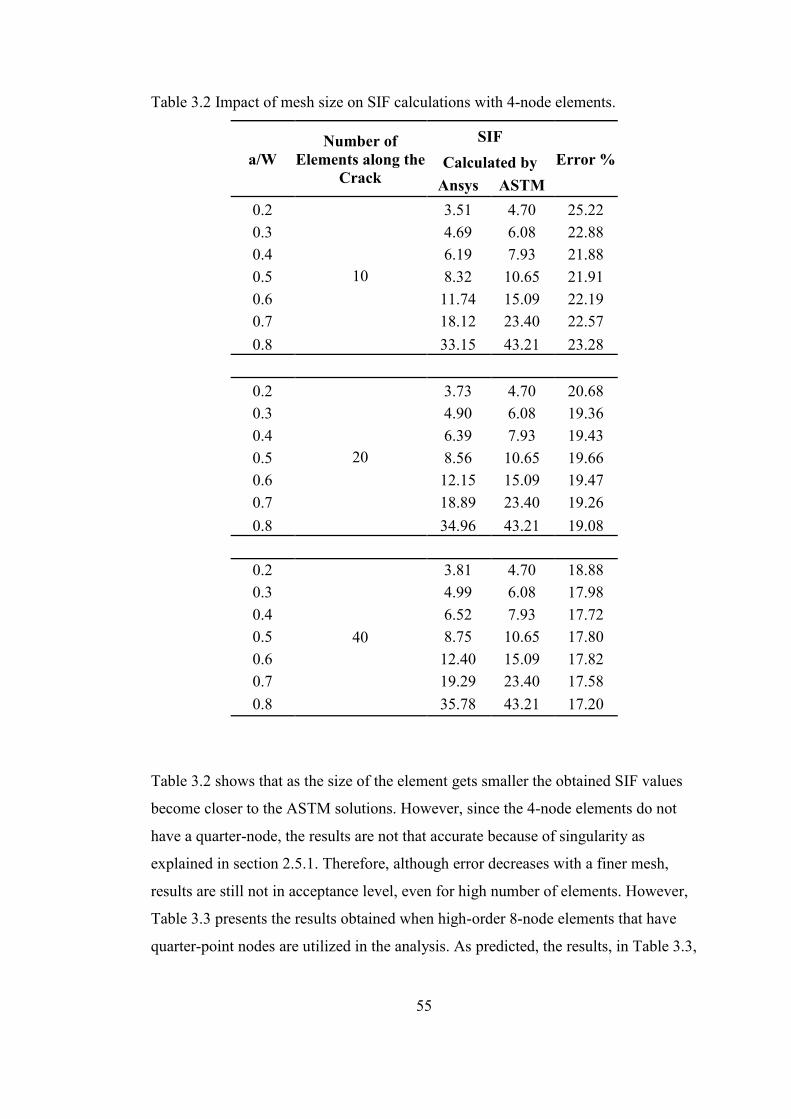
55
Table 3.2 Impact of mesh size on SIF calculations with 4-node elements.
a/W
Number of
Elements along the
Crack
SIF
Error % Calculated by
Ansys ASTM
0.2
10
3.51 4.70 25.22
0.3 4.69 6.08 22.88
0.4 6.19 7.93 21.88
0.5 8.32 10.65 21.91
0.6 11.74 15.09 22.19
0.7 18.12 23.40 22.57
0.8 33.15 43.21 23.28
0.2
20
3.73 4.70 20.68
0.3 4.90 6.08 19.36
0.4 6.39 7.93 19.43
0.5 8.56 10.65 19.66
0.6 12.15 15.09 19.47
0.7 18.89 23.40 19.26
0.8 34.96 43.21 19.08
0.2
40
3.81 4.70 18.88
0.3 4.99 6.08 17.98
0.4 6.52 7.93 17.72
0.5 8.75 10.65 17.80
0.6 12.40 15.09 17.82
0.7 19.29 23.40 17.58
0.8 35.78 43.21 17.20
Table 3.2 shows that as the size of the element gets smaller the obtained SIF values
become closer to the ASTM solutions. However, since the 4-node elements do not
have a quarter-node, the results are not that accurate because of singularity as
explained in section 2.5.1. Therefore, although error decreases with a finer mesh,
results are still not in acceptance level, even for high number of elements. However,
Table 3.3 presents the results obtained when high-order 8-node elements that have
quarter-point nodes are utilized in the analysis. As predicted, the results, in Table 3.3,
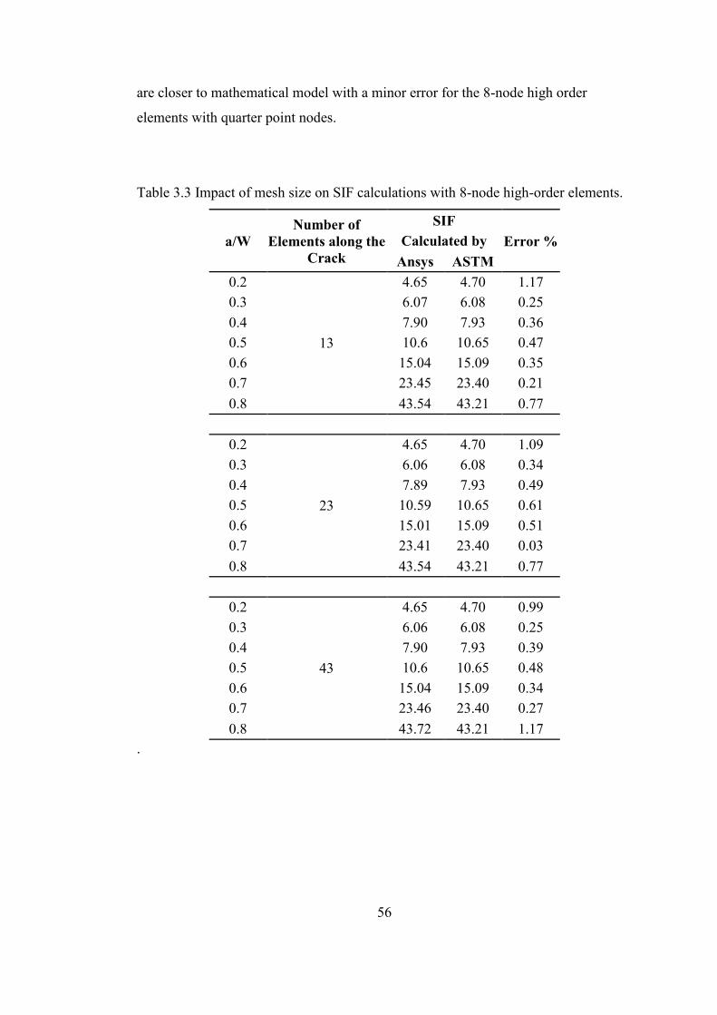
56
are closer to mathematical model with a minor error for the 8-node high order
elements with quarter point nodes.
Table 3.3 Impact of mesh size on SIF calculations with 8-node high-order elements.
a/W
Number of
Elements along the
Crack
SIF
Error % Calculated by
Ansys ASTM
0.2
13
4.65 4.70 1.17
0.3 6.07 6.08 0.25
0.4 7.90 7.93 0.36
0.5 10.6 10.65 0.47
0.6 15.04 15.09 0.35
0.7 23.45 23.40 0.21
0.8 43.54 43.21 0.77
0.2
23
4.65 4.70 1.09
0.3 6.06 6.08 0.34
0.4 7.89 7.93 0.49
0.5 10.59 10.65 0.61
0.6 15.01 15.09 0.51
0.7 23.41 23.40 0.03
0.8 43.54 43.21 0.77
0.2
43
4.65 4.70 0.99
0.3 6.06 6.08 0.25
0.4 7.90 7.93 0.39
0.5 10.6 10.65 0.48
0.6 15.04 15.09 0.34
0.7 23.46 23.40 0.27
0.8 43.72 43.21 1.17
.
57
CHAPTER 4
CRACK PROPAGATION SIMULATION FOR STEEL FIBER
REINFORCED CONCRETE
4
Steel fibers or fibers in general are utilized in concrete to control the tensile cracking
and to increase its toughness. The effects of fiber geometry, fiber properties, fiber
volume on the properties of fiber reinforced concrete are often experimentally
studied (Banthia, 1994), (Oh, 2007). In this part of the thesis numerical simulation of
a FRC beam under bending will be performed. The properties of the materials that
are obtained from literature and the numerical simulation procedure will be explained
in the proceeding sections.
4.1 Material Properties and Finite Element Types.
According to the experimental part of the work carried out by Oh in 2007, the
compressive strength of plain concrete was 36 MPa and the flexural tensile strength
was 4.8 MPa. The dimensions of the beam were 100 x 100 x 400 mm and the span
length was 300 mm as shown in Figure 4.1. The load was applied in four-point
loading condition in displacement control manner and the load versus mid-point
deflection were determined. Specimens with fiber contents of 1% and 1.5% of the
total concrete volume, respectively, were tested.
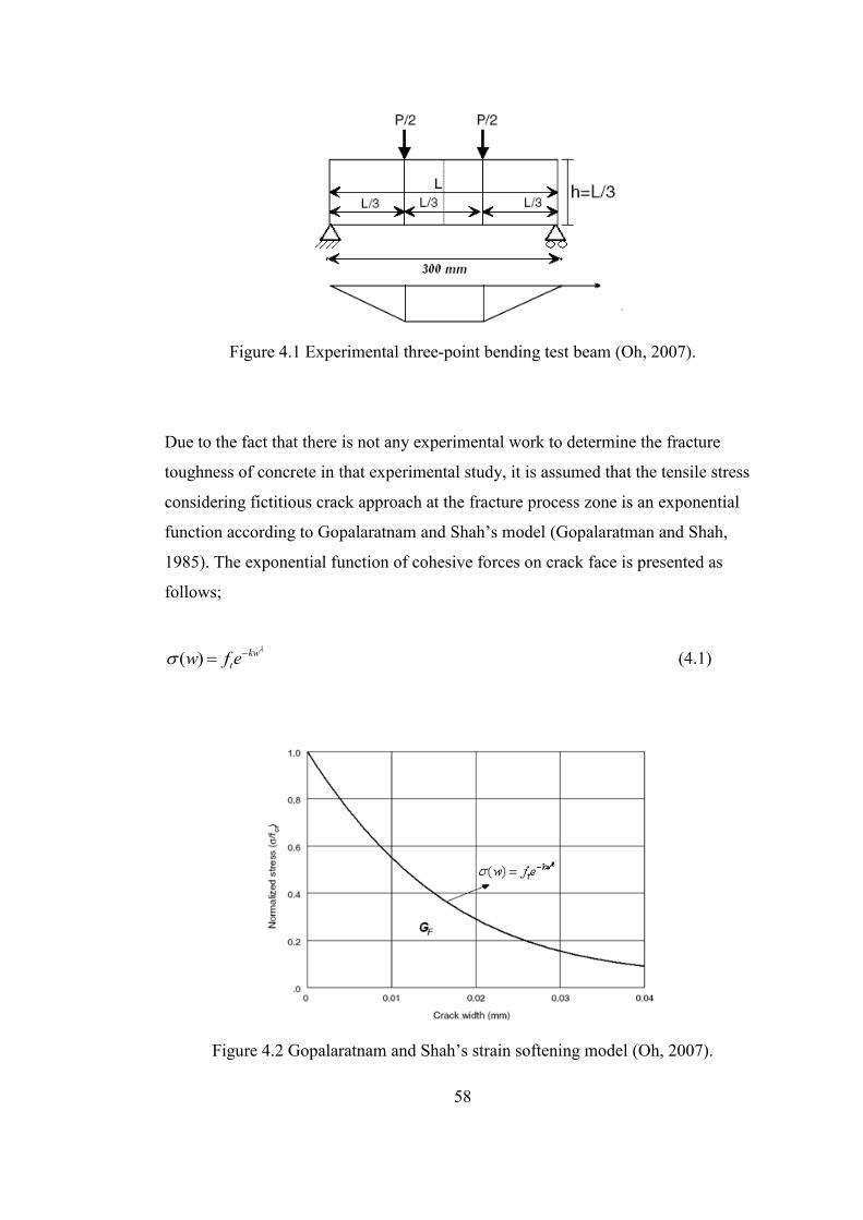
58
Figure 4.1 Experimental three-point bending test beam (Oh, 2007).
Due to the fact that there is not any experimental work to determine the fracture
toughness of concrete in that experimental study, it is assumed that the tensile stress
considering fictitious crack approach at the fracture process zone is an exponential
function according to Gopalaratnam and Shah’s model (Gopalaratman and Shah,
1985). The exponential function of cohesive forces on crack face is presented as
follows;
( ) kw
tw f e
(4.1)
Figure 4.2 Gopalaratnam and Shah’s strain softening model (Oh, 2007).
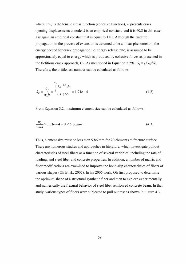
59
where ζ(w) is the tensile stress function (cohesive function), w presents crack
opening displacements at node, k is an empirical constant and it is 60.8 in this case,
λ is again an empirical constant that is equal to 1.01. Although the fracture
propagation in the process of extension is assumed to be a linear phenomenon, the
energy needed for crack propagation i.e. energy release rate, is assumed to be
approximately equal to energy which is produced by cohesive forces as presented in
the fictitious crack approach, GF. As mentioned in Equation 2.29a, GF= (KIC)2/E.
Therefore, the brittleness number can be calculated as follows:
0 1.71 44.8 100
cw
kw
t
f
E
u
f e dwG
S eh
(4.2)
From Equation 3.2, maximum element size can be calculated as follows;
1.71 4 5.862
cw e d mmmd
(4.3)
Thus, element size must be less than 5.86 mm for 20 elements at fracture surface.
There are numerous studies and approaches in literature, which investigate pullout
characteristics of steel fibers as a function of several variables, including the rate of
loading, and steel fiber and concrete properties. In addition, a number of matrix and
fiber modifications are examined to improve the bond-slip characteristics of fibers of
various shapes (Oh B. H., 2007). In his 2006 work, Oh first proposed to determine
the optimum shape of a structural synthetic fiber and then to explore experimentally
and numerically the flexural behavior of steel fiber reinforced concrete beam. In that
study, various types of fibers were subjected to pull out test as shown in Figure 4.3.
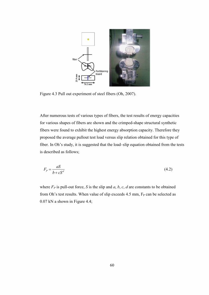
60
Figure 4.3 Pull out experiment of steel fibers (Oh, 2007).
After numerous tests of various types of fibers, the test results of energy capacities
for various shapes of fibers are shown and the crimped-shape structural synthetic
fibers were found to exhibit the highest energy absorption capacity. Therefore they
proposed the average pullout test load versus slip relation obtained for this type of
fiber. In Oh’s study, it is suggested that the load–slip equation obtained from the tests
is described as follows;
P d
aSF
b cS
(4.2)
where FP is pull-out force, S is the slip and a, b, c, d are constants to be obtained
from Oh’s test results. When value of slip exceeds 4.5 mm, FP can be selected as
0.07 kN a shown in Figure 4.4;
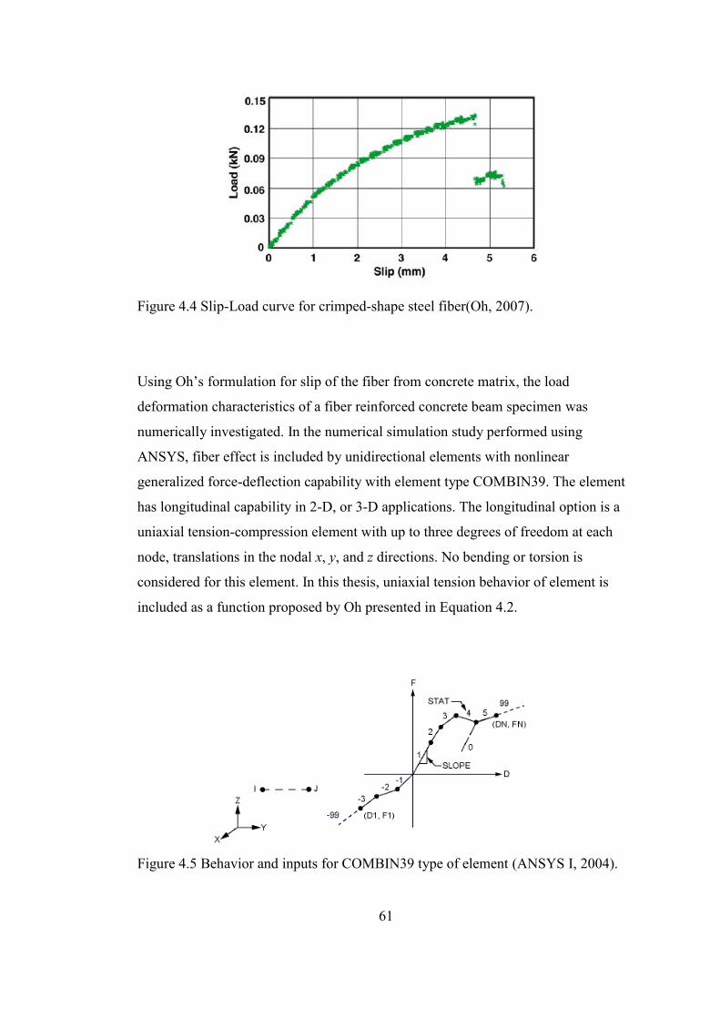
61
Figure 4.4 Slip-Load curve for crimped-shape steel fiber(Oh, 2007).
Using Oh’s formulation for slip of the fiber from concrete matrix, the load
deformation characteristics of a fiber reinforced concrete beam specimen was
numerically investigated. In the numerical simulation study performed using
ANSYS, fiber effect is included by unidirectional elements with nonlinear
generalized force-deflection capability with element type COMBIN39. The element
has longitudinal capability in 2-D, or 3-D applications. The longitudinal option is a
uniaxial tension-compression element with up to three degrees of freedom at each
node, translations in the nodal x, y, and z directions. No bending or torsion is
considered for this element. In this thesis, uniaxial tension behavior of element is
included as a function proposed by Oh presented in Equation 4.2.
Figure 4.5 Behavior and inputs for COMBIN39 type of element (ANSYS I, 2004).

62
Since nonlinear elements have been selected to use in solution, nonlinearity may be
included by using iterative series of linear solution. In ANSYS, the Newton-Rapson
Method or Arc-Length method are used for the solution of nonlinear problems.
Newton-Rapson method is selected to solve the nonlinearity problem.
4.2 Fiber Orientation Factor
P. Soroushian and Cha-Don Lee introduced a formulation for the number of fibers
per unit cross-sectional area for various volume fractions of fibers (Soroushian and
Cha-Don Lee, 1990). They proposed the number of fibers per unit area, N1, as
follows.
1
f
f
VN
A (4.3)
where Af presents the cross-sectional area of steel fibers, Vf is the volume fraction of
steel fibers in the concrete, α is the orientation factor. In an infinitely large volume of
concrete, fibers are expected to be randomly oriented with the same probabilities but
in different directions in space. However, when parallel boundaries exist, the fibers
located near boundaries are in a situation somewhere between three-dimensional and
two-dimensional random orientations. The orientation factor α may be considered as
the effective factor that an arbitrarily-oriented fiber is perpendicular to the crack
plane. Therefore, in 1990, Soroushian and Lee presented a formulation to easily
select an orientation factor for cases with four boundaries as presented in Figure 4.6.
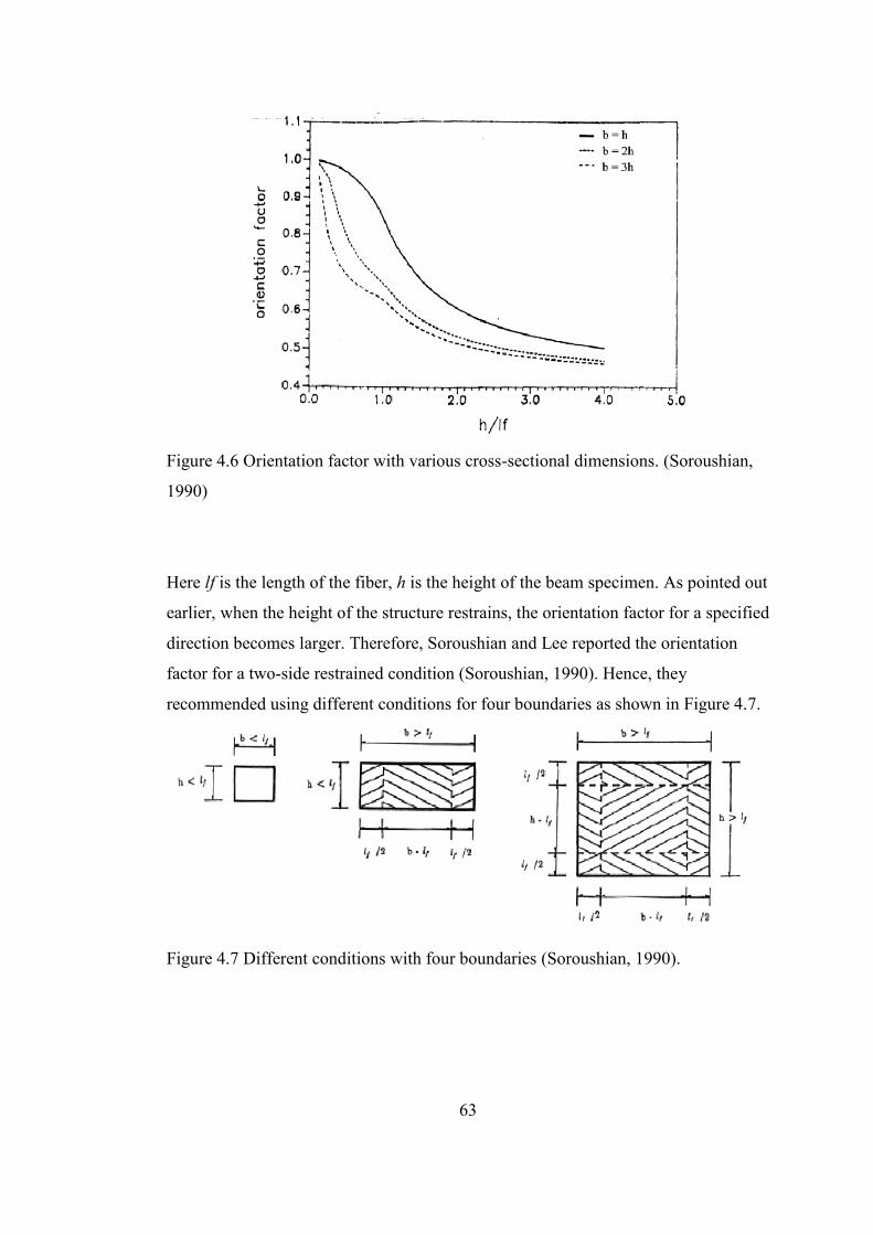
63
Figure 4.6 Orientation factor with various cross-sectional dimensions. (Soroushian,
1990)
Here lf is the length of the fiber, h is the height of the beam specimen. As pointed out
earlier, when the height of the structure restrains, the orientation factor for a specified
direction becomes larger. Therefore, Soroushian and Lee reported the orientation
factor for a two-side restrained condition (Soroushian, 1990). Hence, they
recommended using different conditions for four boundaries as shown in Figure 4.7.
Figure 4.7 Different conditions with four boundaries (Soroushian, 1990).
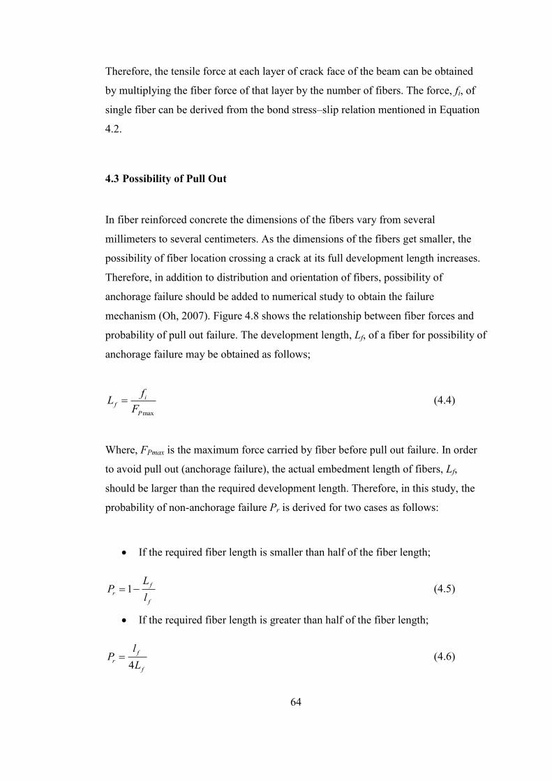
64
Therefore, the tensile force at each layer of crack face of the beam can be obtained
by multiplying the fiber force of that layer by the number of fibers. The force, fi, of
single fiber can be derived from the bond stress–slip relation mentioned in Equation
4.2.
4.3 Possibility of Pull Out
In fiber reinforced concrete the dimensions of the fibers vary from several
millimeters to several centimeters. As the dimensions of the fibers get smaller, the
possibility of fiber location crossing a crack at its full development length increases.
Therefore, in addition to distribution and orientation of fibers, possibility of
anchorage failure should be added to numerical study to obtain the failure
mechanism (Oh, 2007). Figure 4.8 shows the relationship between fiber forces and
probability of pull out failure. The development length, Lf, of a fiber for possibility of
anchorage failure may be obtained as follows;
max
if
P
fL
F (4.4)
Where, FPmax is the maximum force carried by fiber before pull out failure. In order
to avoid pull out (anchorage failure), the actual embedment length of fibers, Lf,
should be larger than the required development length. Therefore, in this study, the
probability of non-anchorage failure Pr is derived for two cases as follows:
If the required fiber length is smaller than half of the fiber length;
1f
r
f
LP
l (4.5)
If the required fiber length is greater than half of the fiber length;
4
f
r
f
lP
L (4.6)
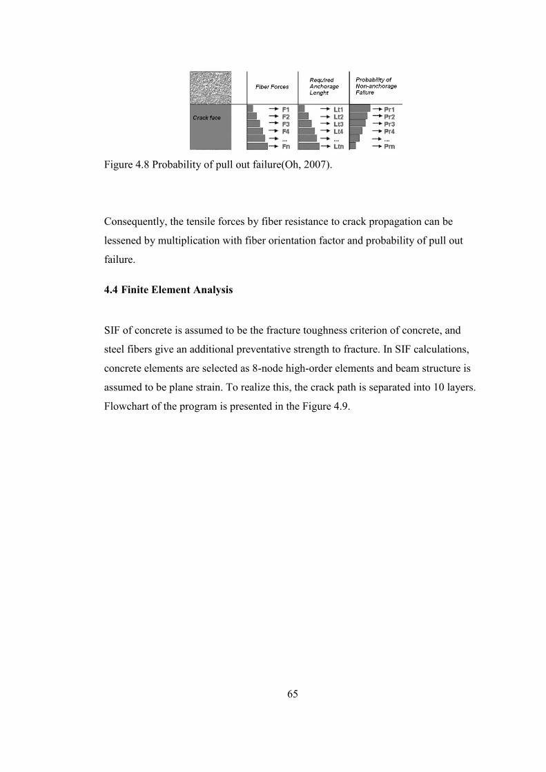
65
Figure 4.8 Probability of pull out failure(Oh, 2007).
Consequently, the tensile forces by fiber resistance to crack propagation can be
lessened by multiplication with fiber orientation factor and probability of pull out
failure.
4.4 Finite Element Analysis
SIF of concrete is assumed to be the fracture toughness criterion of concrete, and
steel fibers give an additional preventative strength to fracture. In SIF calculations,
concrete elements are selected as 8-node high-order elements and beam structure is
assumed to be plane strain. To realize this, the crack path is separated into 10 layers.
Flowchart of the program is presented in the Figure 4.9.
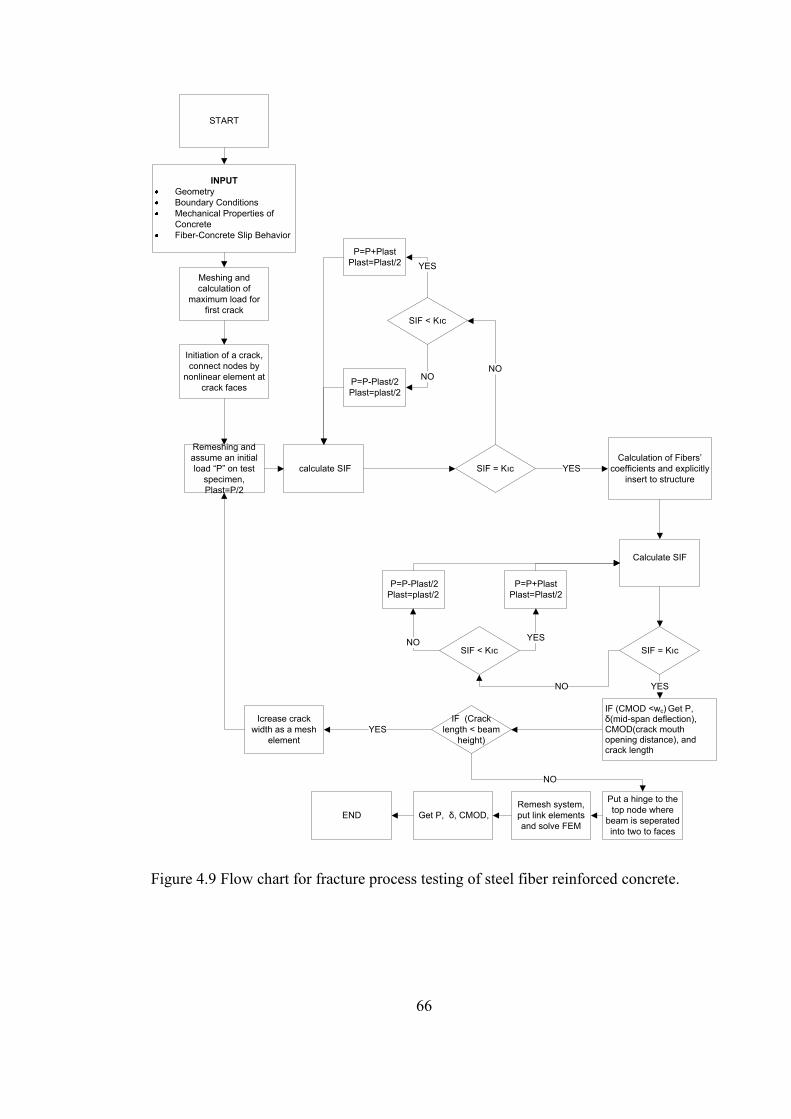
66
START
INPUT
Geometry
Boundary Conditions
Mechanical Properties of
Concrete
Fiber-Concrete Slip Behavior
Meshing and
calculation of
maximum load for
first crack
Initiation of a crack,
connect nodes by
nonlinear element at
crack faces
SIF = Kıc
Calculation of Fibers’
coefficients and explicitly
insert to structure
calculate SIF
Calculate SIF
SIF = Kıc
NO
IF (CMOD <wc) Get P, δ(mid-span deflection), CMOD(crack mouth opening distance), and crack length
YES
Put a hinge to the
top node where
beam is seperated
into two to faces
Remesh system,
put link elements
and solve FEM
P=P-Plast/2
Plast=plast/2
P=P+Plast
Plast=Plast/2
YES
NO
Remeshing and
assume an initial
load “P” on test
specimen,
Plast=P/2
P=P-Plast/2
Plast=plast/2
P=P+Plast
Plast=Plast/2
Icrease crack
width as a mesh
element
IF (Crack
length < beam
height)
YES
NO
Get P, δ, CMOD, END
SIF < Kıc
YES
NO
SIF < Kıc NO
YES
Figure 4.9 Flow chart for fracture process testing of steel fiber reinforced concrete.
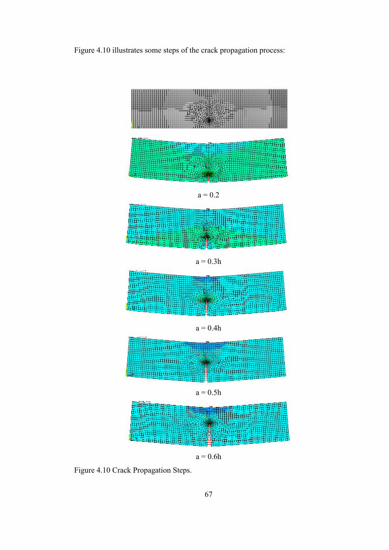
67
Figure 4.10 illustrates some steps of the crack propagation process:
a = 0.2
a = 0.3h
a = 0.4h
a = 0.5h
a = 0.6h
Figure 4.10 Crack Propagation Steps.
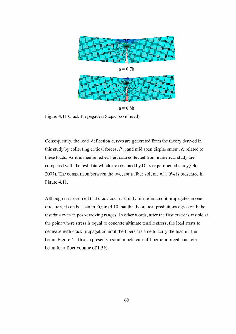
68
a = 0.7h
a = 0.8h
Figure 4.11 Crack Propagation Steps. (continued)
Consequently, the load–deflection curves are generated from the theory derived in
this study by collecting critical forces, Pcr, and mid span displacement, δ, related to
these loads. As it is mentioned earlier, data collected from numerical study are
compared with the test data which are obtained by Oh’s experimental study(Oh,
2007). The comparison between the two, for a fiber volume of 1.0% is presented in
Figure 4.11.
Although it is assumed that crack occurs at only one point and it propagates in one
direction, it can be seen in Figure 4.10 that the theoretical predictions agree with the
test data even in post-cracking ranges. In other words, after the first crack is visible at
the point where stress is equal to concrete ultimate tensile stress, the load starts to
decrease with crack propagation until the fibers are able to carry the load on the
beam. Figure 4.11b also presents a similar behavior of fiber reinforced concrete
beam for a fiber volume of 1.5%.
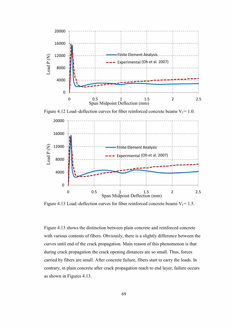
69
Figure 4.12 Load–deflection curves for fiber reinforced concrete beams Vf = 1.0.
Figure 4.13 Load–deflection curves for fiber reinforced concrete beams Vf = 1.5.
Figure 4.13 shows the distinction between plain concrete and reinforced concrete
with various contents of fibers. Obviously, there is a slightly difference between the
curves until end of the crack propagation. Main reason of this phenomenon is that
during crack propagation the crack opening distances are so small. Thus, forces
carried by fibers are small. After concrete failure, fibers start to carry the loads. In
contrary, in plain concrete after crack propagation reach to end layer, failure occurs
as shown in Figures 4.13.
0
4000
8000
12000
16000
20000
0 0.5 1 1.5 2 2.5
Finite Element Analysis
Experimental
Span Midpoint Deflection (mm)
Load
P (
N)
(Oh et al. 2007)
0
4000
8000
12000
16000
20000
0 0.5 1 1.5 2 2.5
Finite Element Analysis
Experimental
Span Midpoint Deflection (mm)
Load
P (
N)
(Oh et al. 2007)
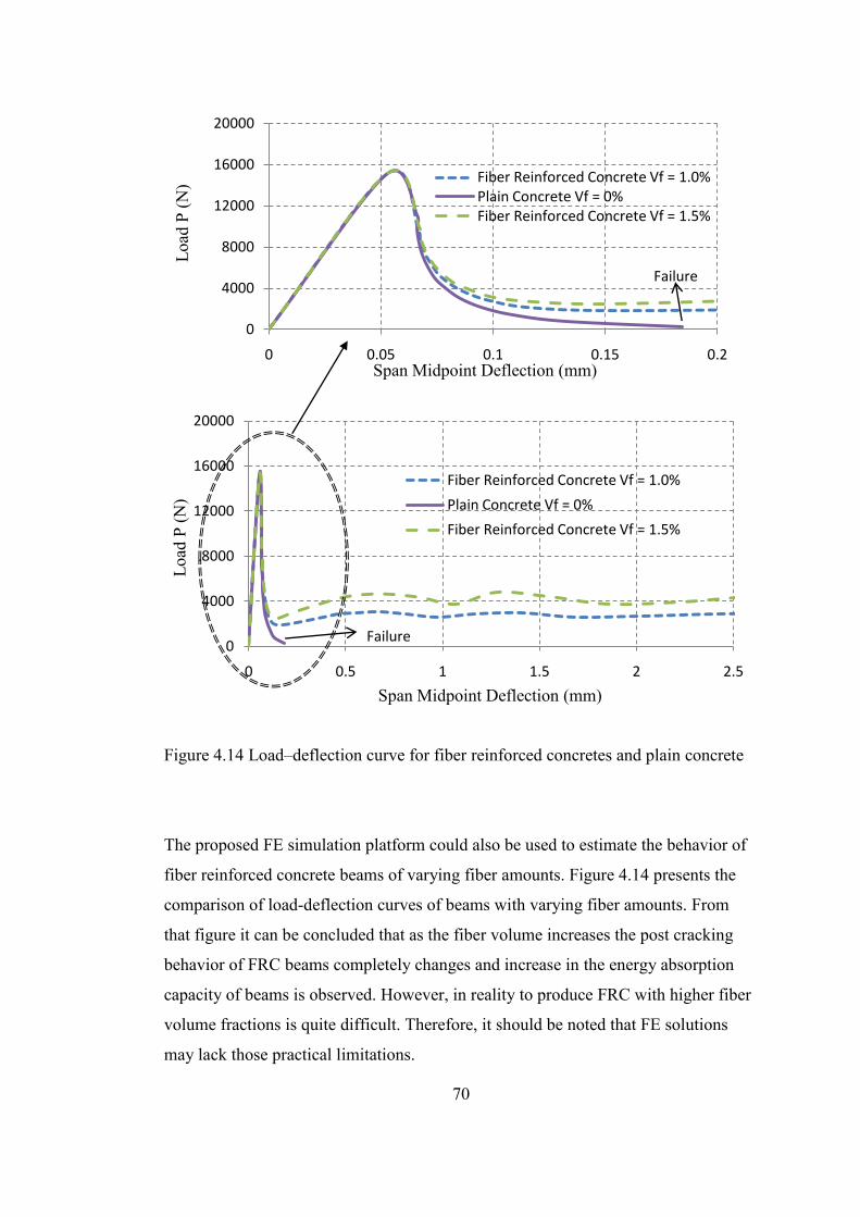
70
Figure 4.14 Load–deflection curve for fiber reinforced concretes and plain concrete
The proposed FE simulation platform could also be used to estimate the behavior of
fiber reinforced concrete beams of varying fiber amounts. Figure 4.14 presents the
comparison of load-deflection curves of beams with varying fiber amounts. From
that figure it can be concluded that as the fiber volume increases the post cracking
behavior of FRC beams completely changes and increase in the energy absorption
capacity of beams is observed. However, in reality to produce FRC with higher fiber
volume fractions is quite difficult. Therefore, it should be noted that FE solutions
may lack those practical limitations.
0
4000
8000
12000
16000
20000
0 0.05 0.1 0.15 0.2
Fiber Reinforced Concrete Vf = 1.0%Plain Concrete Vf = 0%Fiber Reinforced Concrete Vf = 1.5%
Span Midpoint Deflection (mm)
Load
P (
N)
Failure
0
4000
8000
12000
16000
20000
0 0.5 1 1.5 2 2.5
Fiber Reinforced Concrete Vf = 1.0%
Plain Concrete Vf = 0%
Fiber Reinforced Concrete Vf = 1.5%
Span Midpoint Deflection (mm)
Load
P (
N)
Failure
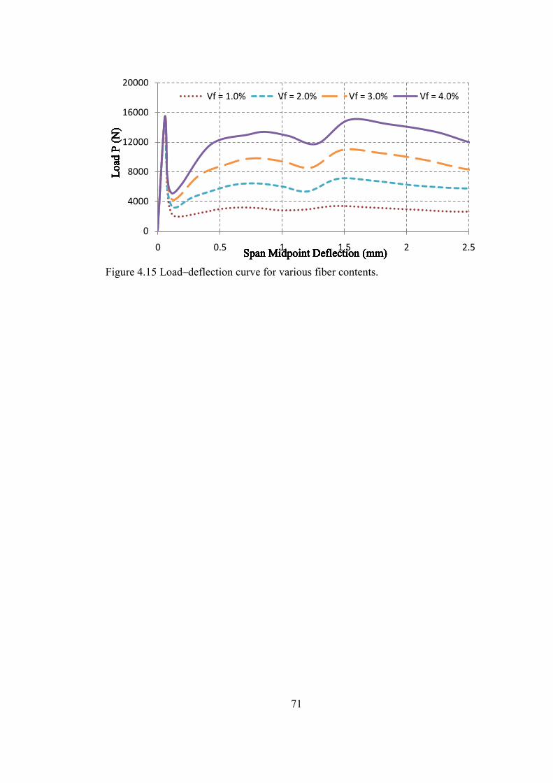
71
Figure 4.15 Load–deflection curve for various fiber contents.
0
4000
8000
12000
16000
20000
0 0.5 1 1.5 2 2.5
Vf = 1.0% Vf = 2.0% Vf = 3.0% Vf = 4.0%
Span Midpoint Deflection (mm)
Load
P (
N)
Span Midpoint Deflection (mm)
Load
P (
N)
Span Midpoint Deflection (mm)
Load
P (
N)
Span Midpoint Deflection (mm)
Load
P (
N)
Span Midpoint Deflection (mm)
Load
P (
N)
Span Midpoint Deflection (mm)
Load
P (
N)
Span Midpoint Deflection (mm)
Load
P (
N)
Span Midpoint Deflection (mm)
Load
P (
N)

72
CHAPTER 5
SUMMARY AND CONCLUSIONS
5
5.1 Summary
The purpose of the present study was to develop a finite element simulation tool for
the fracture process of fiber reinforced concrete beam specimens subjected to
flexural bending test. Therefore, the efficiency of mesh refinement has been
presented in early chapters. Then, the slip-load mechanism of the fibers and their
probabilities to resist tensile force are referenced. Unfortunately, since an
experimental study is not presented in this thesis, Oh’s experimental work is selected
for the comparative part of the study (Oh B. H., 1992). Finally, two FE models and
experimental work were used to verify the effect of steel fibers on fracture process
and post process.
5.2 Conclusions
The following conclusions can be drawn from the results of this study:
1. As in all finite element calculations, mesh size and element type are the most
important part of calculation. In FE model of fracture of concrete, if SIF or
energy release rate is used as criterion on fracture, special elements must be
used. Otherwise miscalculation and unexpected errors may come up.
Therefore, 4-node elements should not be selected in this case. Additionally,
mesh size and brittleness number should be considered for accurate results.
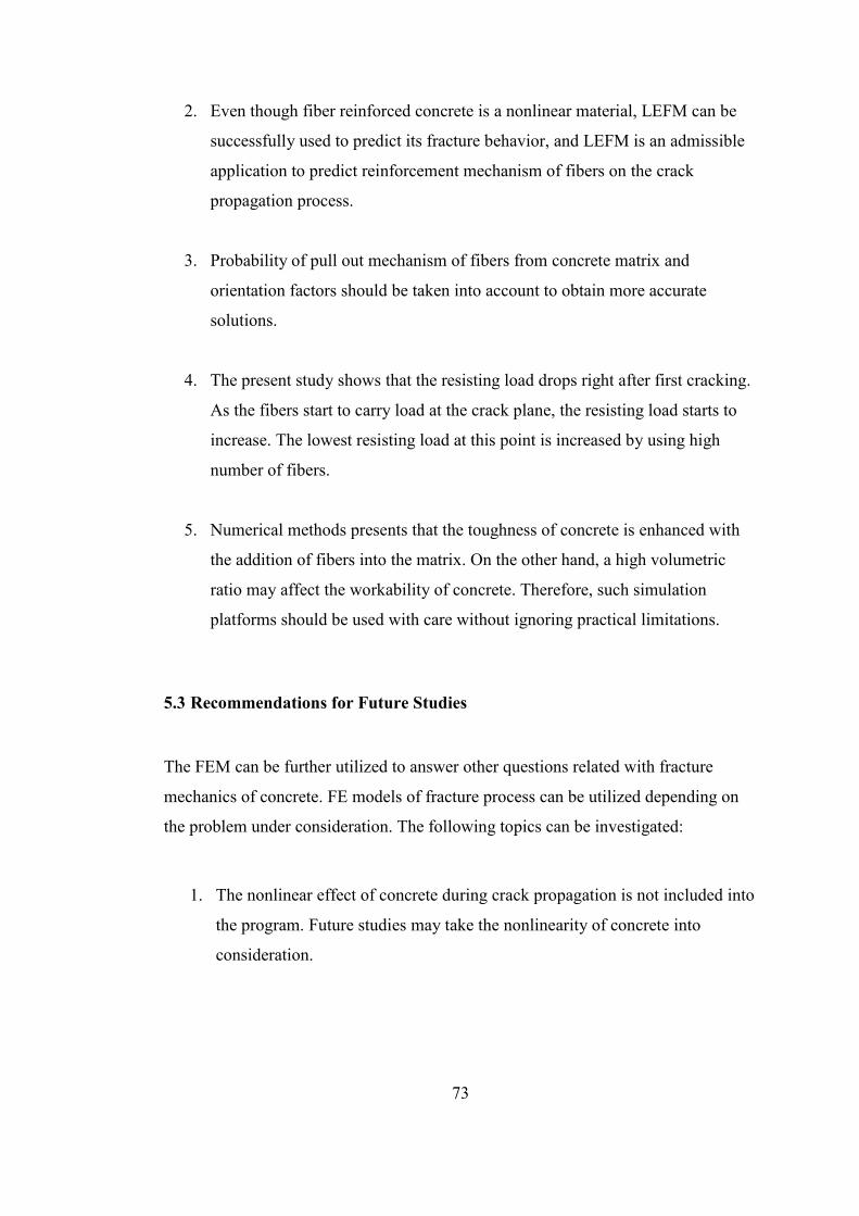
73
2. Even though fiber reinforced concrete is a nonlinear material, LEFM can be
successfully used to predict its fracture behavior, and LEFM is an admissible
application to predict reinforcement mechanism of fibers on the crack
propagation process.
3. Probability of pull out mechanism of fibers from concrete matrix and
orientation factors should be taken into account to obtain more accurate
solutions.
4. The present study shows that the resisting load drops right after first cracking.
As the fibers start to carry load at the crack plane, the resisting load starts to
increase. The lowest resisting load at this point is increased by using high
number of fibers.
5. Numerical methods presents that the toughness of concrete is enhanced with
the addition of fibers into the matrix. On the other hand, a high volumetric
ratio may affect the workability of concrete. Therefore, such simulation
platforms should be used with care without ignoring practical limitations.
5.3 Recommendations for Future Studies
The FEM can be further utilized to answer other questions related with fracture
mechanics of concrete. FE models of fracture process can be utilized depending on
the problem under consideration. The following topics can be investigated:
1. The nonlinear effect of concrete during crack propagation is not included into
the program. Future studies may take the nonlinearity of concrete into
consideration.
74
2. In new generation finite element programs, there is special element which is
called “Cohesive Zone Material”. These kinds of elements provide fracture
debonding more easily. With this kind of modeling, fibers’ pull out
mechanism of fibers in concrete may be directly introduced.
75
REFERENCES
6
ACI. (2009). Finite Element Analysis of Fracture in Concrete Structures. ACI The
2009 Manual of Concrete Practice , Part 5. 446.3R-97.
Anderson, T. L. (2005). Fracture mechanics: fundamentals and applications. CRC
Press.
ANSYS, I. a. (2007, january). Programer's Manual for Ansys.
ANSYS, I. (2004). Documentation for ANSYS. Southpointe.
Araújo, T. B. (2000). Numerical estimation of fracture parameters in elastic and
elastic-plastic analysis. European Congress on Computational Methods in Applied
Sciences and Engineering , ECCOMAS, Barcelona.
ASTM. (2005). Standard Method of Test for Plane-Strain Fracture Toughness of
Metallic Material. Mannual, American Society for Testing and Materials.
Banthia, N. T. (1994). Concrete reinforced with deformed steel fibers, part I: bond-
slip mechanisms. ACI Materials Journal , 435-446.
Bažant, Z. P. (2002). Concrete Fracture Models: testing and practice. Engineering
Fracture Mechanics , 165-205.
Bažant, Z. P. (1983). Crack Band Theory for Fracture Model for Concrete. Materials
and Structures, RIMEL, Vol. 6 , 155-177.
Bažant, Z. P. (1990). Determination of Fracture Energy, Process Zone Lenght and
Brittleness Number from Size Effect, With application to rock and concrete.
Ineternational Journal of Fracture, Vol. 44 , 111-131.
Bažant, Z. P. (1976). Instability, Ductility and Size Effect in Strain-Softening
Concrete. J. Engineering Mechanics , 331-334.
76
Bažant, Z. P. (1984). Size Effect in Blunt Fracture:Concrete, Rock, Metal. Journal of
Engineering Mechanics, ASCE, Vol.110, No. 4 , 518-535.
Bažant, Z. P.-G. (2002). Statistical prediction of fracture parameters of concrete and
implications for choice of testing standard. Cement and Concrete Research , 529-
556.
Carpinteri, A. P. (1992). Applications of Fracture Mechanics to Reinforced Concrete.
Elsevier Applied Science, London , XIV + 616.
Carpinteri, A. P. (1999). Minimum Reinforcement in Concrete Science. Oxford ,
VUI + 203.
Carpinteri, A. P. (2007, 11 14). Innovative Learning and Training on Fracture.
Retrieved from http://www.iltof.org/
Carpinteri, A. (1984). Stability of fracturing process in R.C. beams. Journal of I
Structural Engineering (ASCE), Vol. 110 .
Eftis, J. A. (1972). On the Modified Westergaard Equations for Certain Plane Crack
Problems. Int J. Fracture Mechanics , 383-392.
Gopalaratman, V. S. (1985). Softening Response of Plain Concrete in Direct
Tension. ACI Journal , 82, 310-323.
Hillerborg, A. M. (1976). Analysis of crack formation and crack growth in concrete
by means of fracture mechanics and finite Elements. Cement and Concrete Research,
Vol 6, No 6 , 773-782.
Irwin, G. R. (1960). Plastic zone nera a Crack and Fracture Toughness. in
Proceeding of the Seventh Sagamore Ordnance MAterials Conference, Syracuse
University , IV-60.
Jenq, Y. S. (1985). A Two Parameter Fracture Model for Concrete. Journal of
Engineering Mechanics, Vol.111, No. 4 , 1227-1241.
77
Jenq, Y. S. (1985). Two parameter fracture model for concrete. J. Eng. Mech. , 1227-
1241.
Kaplan, M. F. (1961). Crack propagation and the fracture of concrete. ACI journal ,
591-610.
Karihaloo, B. N. (1989). An improved effective crack model for the determination of
fracture toughness of cocnrete. Cem. Concr. Res. , 603-610.
Kesler, C. N. (1972). Fracture mechanics-its applicability to concret, Proceedings of
the International Conference on the Mechanical Behaviour of Materials. Society of
Materials Science , 113-124.
Kim J.H., P. G. (2002). Mixed-mode Fracture of Orthotropic Functionally Graded
Materials Using Finite Elements and the Modified Crack Closure Method.
Engineering Fracture Mechanics , Vol. 69 1557-1586.
Oh, B. H. (1992). Flexural analysis of reinforced concrete beams containing steel
fibers. ASCE J Structral Engineering , 118(10):2691–8.
Oh, B. H. (2007). Fracture behavior of concrete members reinforced. Engineering
Fracture Mechanics , 243–257.
Planas, J. E. (1992). Fracture Criteria for Concrete: Mathematical Approximations
and Experimental Validation. 35, 87-94.
Rashid, Y. R. (1968). Ultimate Strength Analysis of Presetressed Concrete Pressure
Vessels . Nuclear Engineeering and Design , 379-386.
Rice, J. R. (1968). A Path Independent and the approximate analysis of strain
concentration by notches and cracks. Journal of Applies Mechanics , 379-286.
Robert D. Cook, D. S. (2001). Concept and Applications of Finite Element Analysis.
Madison: Wiley.
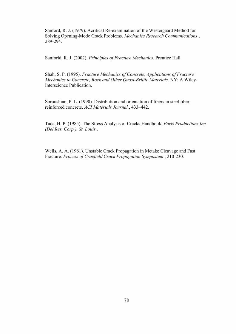
78
Sanford, R. J. (1979). Acritical Re-examination of the Westergaard Method for
Solving Opening-Mode Crack Problems. Mechanics Research Communications ,
289-294.
Sanforld, R. J. (2002). Principles of Fracture Mechanics. Prentice Hall.
Shah, S. P. (1995). Fracture Mechanics of Concrete, Applications of Fracture
Mechanics to Concrete, Rock and Other Quasi-Brittle Materials. NY: A Wiley-
Interscience Publication.
Soroushian, P. L. (1990). Distribution and orientation of fibers in steel fiber
reinforced concrete. ACI Materials Journal , 433–442.
Tada, H. P. (1985). The Stress Analysis of Cracks Handbook. Paris Productions Inc
(Del Res. Corp.), St. Louis .
Wells, A. A. (1961). Unstable Crack Propagation in Metals: Cleavage and Fast
Fracture. Process of Cracfield Crack Propagation Symposium , 210-230.

79
8 APPENDIX A
MESH RESOLUTIONS
a) a/W=0.2
b) a/W=0.3
c) a/W=0.4
Figure A.8.1 Mesh resolution according to 10 elements at fracture surface.
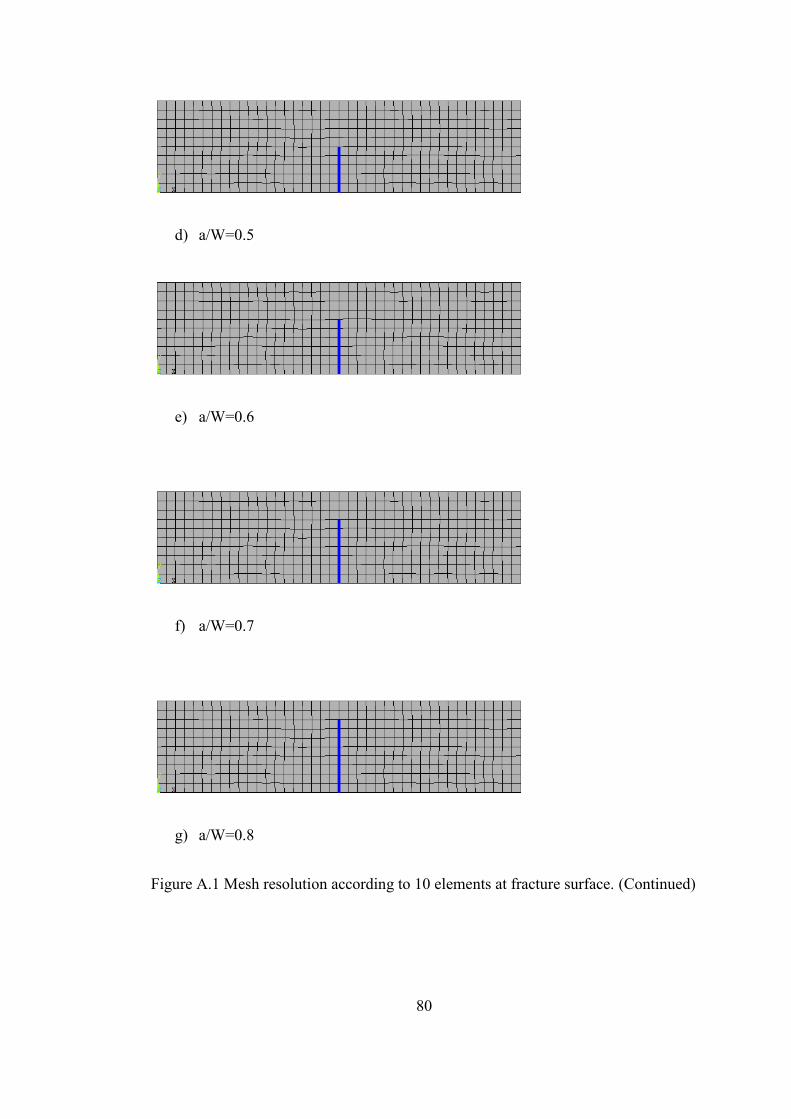
80
d) a/W=0.5
e) a/W=0.6
f) a/W=0.7
g) a/W=0.8
Figure A.1 Mesh resolution according to 10 elements at fracture surface. (Continued)
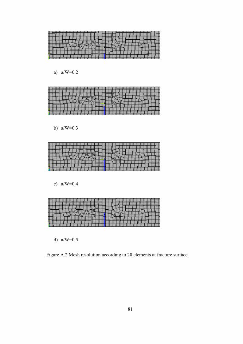
81
a) a/W=0.2
b) a/W=0.3
c) a/W=0.4
d) a/W=0.5
Figure A.2 Mesh resolution according to 20 elements at fracture surface.
82
e) a/W=0.6
f) a/W=0.7
g) a/W=0.8
Figure A.2 Mesh resolution according to 20 elements at fracture surface. (Continued)
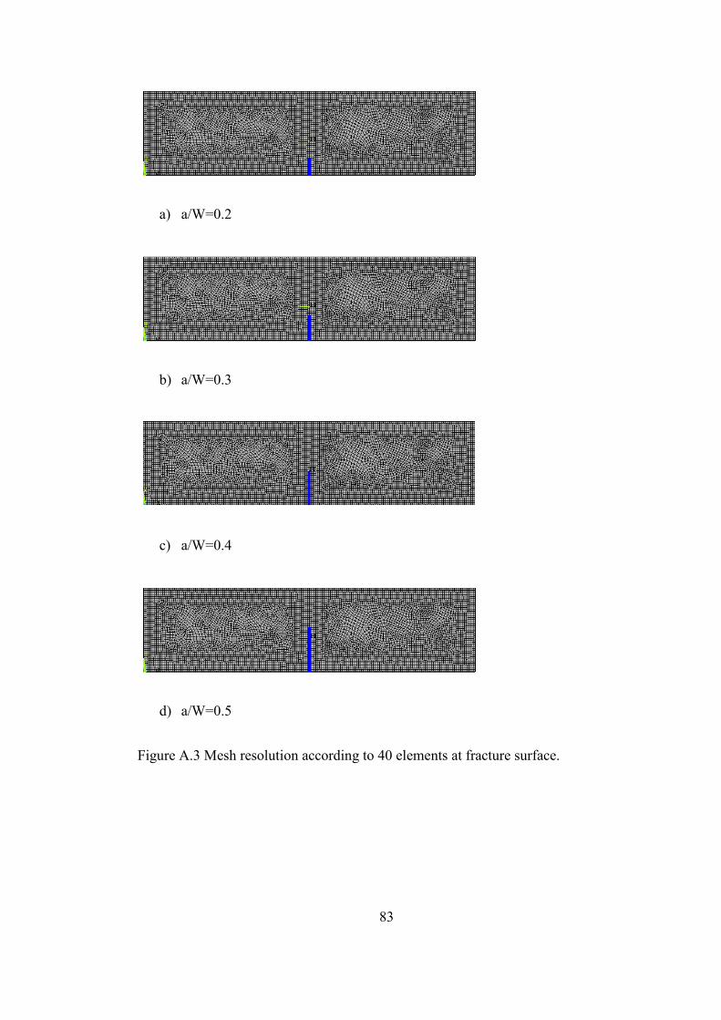
83
a) a/W=0.2
b) a/W=0.3
c) a/W=0.4
d) a/W=0.5
Figure A.3 Mesh resolution according to 40 elements at fracture surface.

84
e) a/W=0.6
f) a/W=0.7
g) a/W=0.8
Figure A.3 Mesh resolution according to 40 elements at fracture surface. (Continued)

85
a) a/W=0.2
b) a/W=0.3
c) a/W=0.4
d) a/W=0.5
Figure A.4 Mesh resolution according to 13 elements at fracture surface.
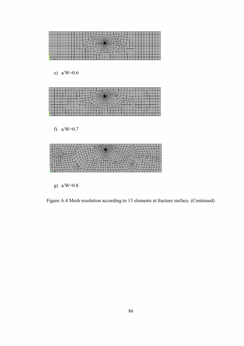
86
e) a/W=0.6
f) a/W=0.7
g) a/W=0.8
Figure A.4 Mesh resolution according to 13 elements at fracture surface. (Continued)
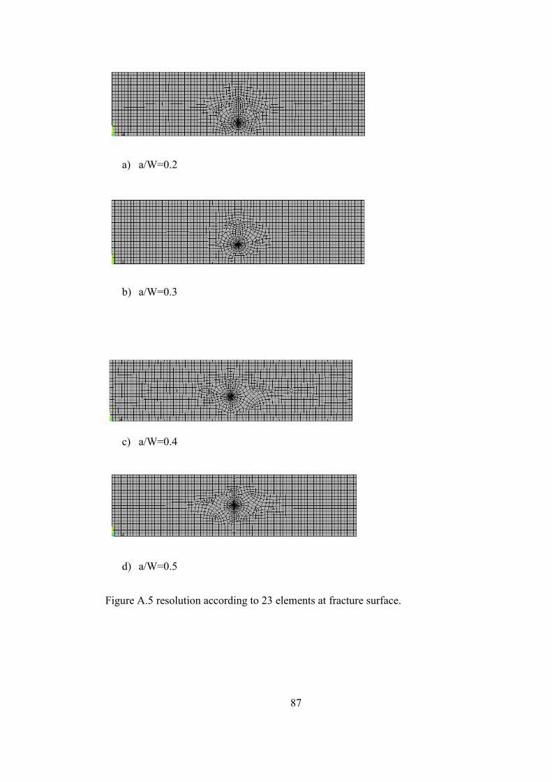
87
a) a/W=0.2
b) a/W=0.3
c) a/W=0.4
d) a/W=0.5
Figure A.5 resolution according to 23 elements at fracture surface.
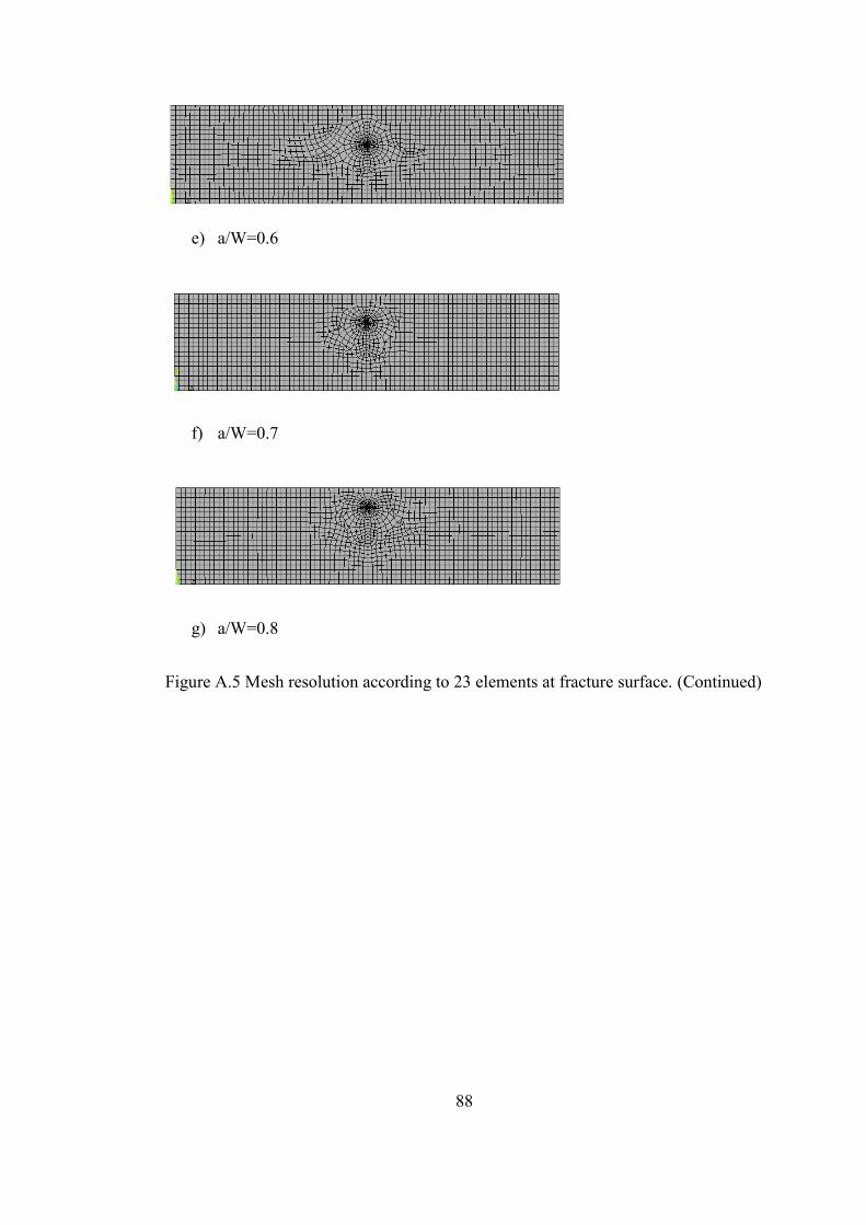
88
e) a/W=0.6
f) a/W=0.7
g) a/W=0.8
Figure A.5 Mesh resolution according to 23 elements at fracture surface. (Continued)
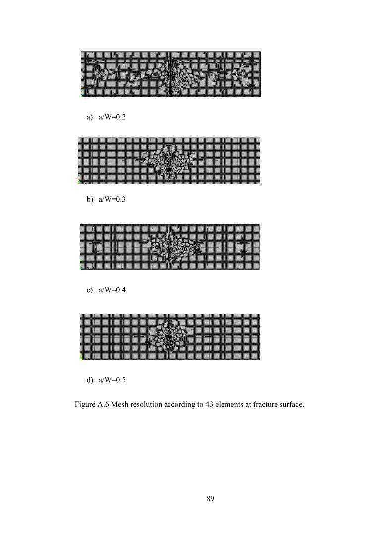
89
a) a/W=0.2
b) a/W=0.3
c) a/W=0.4
d) a/W=0.5
Figure A.6 Mesh resolution according to 43 elements at fracture surface.
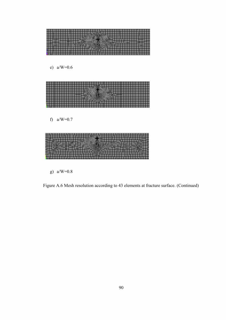
90
e) a/W=0.6
f) a/W=0.7
g) a/W=0.8
Figure A.6 Mesh resolution according to 43 elements at fracture surface. (Continued)