FINITE ELEMENT MODELLING OF THERMO … words: thermo-elastoplasticity, water saturated porous...

Journal of Theoretical and Applied Mechanics, Sofia, 2008, vol. 38, Nos 1–2, pp. 7–24

FINITE ELEMENT MODELLING OF

THERMO-ELASTO-PLASTIC WATER SATURATED

POROUS MATERIALS*

Lorenzo Sanavia

Dipartimento di Costruzioni e Trasporti, Universita degli Studi di Padova,

Via Marzolo 9, 35-131 Padova, Italy,

e-mail:[email protected]

Bertrand Francois

Soil Mechanics Laboratory, Ecole Polytechnique Federale Lausanne, EPFL,

1015 Lausanne, Switzerland,


Roberto Bortolotto, Loris Luison

Dipartimento di Costruzioni e Trasporti, Universita degli Studi di Padova,

Via Marzolo 9, 35-131 Padova, Italy,

e-mails:[email protected], [email protected]

Lyesse Laloui

Soil Mechanics Laboratory, Ecole Polytechnique Federale Lausanne, EPFL,

1015 Lausanne, Switzerland,


Dedicated to Professor Bernhard A. Schrefler on the occasion of his 65th

birthday

[Received 10 July 2007. Accepted 25 February 2008]

Abstract.The purpose of this paper is to present a new finite elementformulation for the hydro-thermo-mechanical analysis of elasto-plasticmultiphase materials based on Porous Media Mechanics.

To this end, the ACMEG-T thermo-plastic constitutive model for sat-urated soils has been implemented in the finite element code COMES-GEO.

Validation of the implemented model is made by selected comparison

*The authors would like to thank the University of Padua (UNIPD 60A09-5407/06), theFoundation “Cassa di Risparmio di Padova e Rovigo” and the Swiss State Secretariat forEducation and Research SER (Grant OFES C04.0021) for their financial support.

8 L. Sanavia, B. Francois, R. Bortolotto, L. Luison, L. Laloui

between model simulation and experimental results for different combina-tions of thermo-hydro-mechanical loading paths. A case of non-isothermalelasto-plastic consolidation is also shown.Key words: thermo-elastoplasticity, water saturated porous materials,finite element method, isotropic compression test, triaxial test, consolida-tion.

1. Introduction

In recent years, increasing interest in thermo-hydro-mechanical analysisof geomaterials is observed, because of a wide spectrum of their engineeringapplications. Typical examples belong to Environmental Geomechanics, wheresome challenging problems are of interest, as for example the case of the nuclearwaste isolation and of geothermal structures.

A step in the development of a suitable physical, mathematical andnumerical model for the simulation of geo-environmental engineering problemsis presented here. To this end, the general ACMEG-T thermo-elastoplasticconstitutive model for saturated soils [1], [2] has been implemented in thefinite element code COMES-GEO for the analysis of non-isothermal elasto-plastic porous materials [3].

In this paper we summarize the mathematical formulation for non-isothermal elasto-plastic water saturated porous materials in Section 2. Thematerial is considered as made of a solid phase and open pores, which are filledwith one fluid, and is modelled as a deforming porous continuum where heatconduction and convection and water advection are taken into account [4], [5].The elasto-plastic behaviour of the solid skeleton is assumed homogeneous andisotropic; the effective stress state is limited by two temperature dependentyield surfaces, with non associated plastic flow, as presented in Section 3.The macroscopic balance equations are discretized in space and time withinthe finite element method for coupled problems, e.g. [4]. In particular, aGalerkin procedure is used for the discretisation in space, and the GeneralisedTrapezoidal Method for the time integration (see Section 5). Small strains andquasi-static loading conditions are assumed.

Validation of the implemented model by selected comparison betweenmodel simulation and experimental results for different combinations of thermo-hydro-mechanical loading paths is presented in Section 6. A case of non-isothermal elastic and elasto-plastic consolidation is described.

A review of non-isothermal thermo-hydro-mechanical models and ofthermo-elasto-plastic constitutive formulations for soils is beyond the scope ofthis paper; the interested reader can find it in [3], [4] and [1], [2], respectively.

Finite Element Modelling of Thermo-Elasto-Plastic Water. . . 9

2. Macroscopic balance equations

A full mathematical model necessary to simulate Thermo-Hydro-Me-chanical (THM) transient behaviour of fully and partially saturated porousmedia was developed in [4], [5] and [6] using averaging theories following [7] (seealso [8]). The model for water saturated porous materials is briefly summarizedin the present section for sake of completeness.

The porous medium is treated as two-phase system composed of thesolid skeleton (s) with open voids filled with water (w).

At the macroscopic level the porous material is modelled by a substitutecontinuum of volume B with boundary ∂B that simultaneously fills the entiredomain, instead of the real fluid and the solid which fill only a part of it. Inthis substitute continuum each constituent π has a reduced density which isobtained through the volume fraction ηπ(x, t) = dvπ(x, t)/dv(x, t), where x isthe vector of the spatial coordinates and t is the current time (π = s, w). Heatconduction, heat convection and water flow due to pressure gradient inside thepores are taken into account. The solid is deformable and non-polar, and thefluid, solid and thermal fields are coupled. Local thermal equilibrium betweensolid matrix and liquid phase is assumed. The state of the medium is describedby pore water pressure pw, absolute temperature T and displacements of thesolid matrix u. Pore pressure is defined as compression positive for water,while stress is defined as tension positive for the solid phase.

Before presenting the balance equations used in the present case, it isuseful to mention that the full mathematical model and its implementationin the COMES-GEO finite element code consider the soil as a non-isothermalthree-phase media in which not only water but also a gas phase may fill thevoid space. In this complete formulation, which is not addressed here, the gasphase is modelled as an ideal gas mixture composed of dry air and water vapour.Phase changes of water (evaporation-condensation, adsorption-desorption) andlatent heat transfer are considered [4], [5], [6], [8]. A recent development whichconsiders the air dissolved in the liquid phase and its desorption at lower waterpressure is presented in [9].

The balance equations of the implemented model are now summarized.These equations are obtained assuming the porous medium to be constitutedof incompressible solid and water constituent; the process is considered asquasi-static and developed in the geometrically linear framework.

The linear momentum balance equation of the mixture in terms ofeffective Cauchy’s stress σ ′(x, t) assumes the form,

(1) div(

σ′ − pw 1)

+ ρg = 0,


where ρ = [1 − n] ρs + nρw is the density of the mixture, n(x,t) the porosity,g is the gravity acceleration vector and 1 the second order identity tensor.

The mass conservation equation for the water is,

(2) ρw div vs − div

(

ρw k

µw[grad (pw) − ρwg]

)

− ρwβsw

∂T

∂t= 0,

where vs is the solid velocity, k(x, t) is the intrinsic permeability tensor andµw(x, t) the water viscosity. βsw(x, t) = [1 − n]βs + nβw is the cubic thermalexpansion coefficient of the medium, βs and βw being the solid and water cubicthermal expansion coefficient, respectively. In equation (2), the water flux hasbeen described using the Darcy law.

The energy balance equation of the mixture has the following form,(3)

(ρCp)eff∂T

∂t−

(

ρwCwp

k

µw[grad (pw) − ρwg]

)

· grad T − div (χeff grad T ) = 0,

where (ρCp)eff = (1 − n) ρsCsp + nρwCw

p is the effective thermal capacity ofporous medium, Cs

p and Cwp the specific heat of solid and water, respectively,

and χeff the effective thermal conductivity of the porous medium. This bal-ance equation takes into account the heat transfer through conduction andconvection (see [4], [5]) and neglects the terms related to the mechanical workinduced by density variations due to temperature changes of the phases andinduced by volume fraction changes.

3. Constitutive equations

The thermo-elastoplastic behaviour of the solid skeleton is described bythe general ACMEG-T thermo-plastic constitutive model for water saturatedsoils developed in [1], [2], [10] within the rate-independent elasto-plasticitytheory for geometrically linear problems.

The most relevant experimental results for the constitutive descriptionof the soil behaviour will be summarized in the following, before the descriptionof the constitutive model (see e.g. [2] for a comprehensive description).

When studying thermo-mechanical behaviour of soil, some specific ex-perimental observations must be considered in the constitutive development. Inparticular, irreversible processes induced by temperature changes may inducethermo-plastic processes in soils. These irreversible effects strongly depend onthe stress level measured in terms of OverConsolidation Ratio (OCR). UnderNormally Consolidated conditions (NC), soils contracts when it is heated and


a significant part of this deformation is irreversible upon cooling. The behav-iour over the whole cycle indicates the irreversibility of strain due to thermalloading, which is representative of thermal hardening. On the contrary, thehighly overconsolidated states produce mainly reversible dilation when heated.Between these states, an intermediate one (low OCR) first produces dilation,then a tendency toward contraction on heating paths.

In addition, several results from the literature show a decrease in thepreconsolidation pressure with increasing temperature. Finally, under undrai-ned conditions, when soil is heated, the higher thermal expansion of water thanthat of the solid skeleton induces pore water pressure increase. Indeed, a tem-perature increase tends to enhance the pore space of the material proportion-ally to the thermal expansion coefficient of the solid skeleton. Nevertheless, thiseffect is more than counterbalanced by the thermal dilation of water. Moreover,when the soil tends to collapse during heating (due to thermo-plastic behav-iour of NC soils), the undrained conditions make the decrease of pore spaceimpossible, which provokes an additional increase in pore water pressure.

The ACMEG-T model considers a non-linear thermo-elasticity coupledwith a multi-dissipative thermo-plasticity in order to reproduce all the thermo-mechanical features of behaviour exposed above.

The elastic part of the deformation is expressed as following:

(4) dεe = D−1dσ′ + βTdT,

D is the mechanical elastic tensor defined by the non-linear bulk and shearmodulus, K and G, respectively,

(5) K = Kref

(

p′

p′ref

)ne

, G = Gref

(

p′

p′ref

)ne

,

p′ is the effective mean stress, ne the non-linear elasticity exponent, p′ref thereference pressure, Kref and Gref the bulk and shear modulus at the referencepressure, respectively. βT is the thermal expansion tensor. Considering anisotropic thermal dilatation, one can express the thermal expansion tensor as

βT =1

3βs 1 with βs being the volumetric thermal expansion coefficient of the

solid skeleton.

The material plasticity is induced by two coupled mechanisms: anisotropic and a deviatoric mechanism. The yield functions of the two me-chanical thermo-plastic mechanisms, fiso and fdev, representing the isotropic


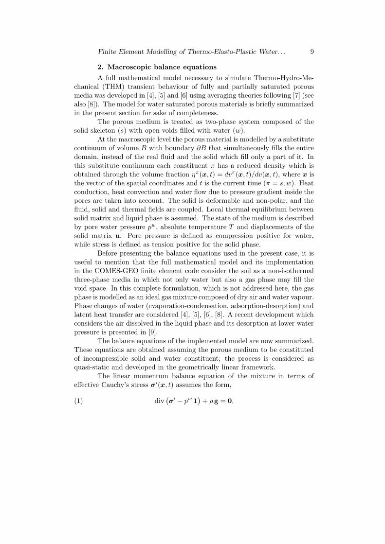
and deviatoric yield limits, respectively, restricting the effective stress stateσ′(x, t), take the following expressions (Fig. 1):

(6) fiso = p′ − p′criso, fdev = q − Mp′(

1 − b lndp′

p′c

)

rdev = 0,

where q is the deviatoric stress. Each of the yield limits evolves through thegeneration of plastic strains. During loading, the volumetric plastic straingoverns the evolution of p′c and riso, while deviatoric plastic strains control theevolution of rdev.

Fig. 1. Yield limits for the ACMEG-T thermo-mechanical elasto-plastic framework.q: shear stress, p′: mean effective stress, T : temperature, p′

c: critical pressure

The preconsolidation pressure, p′c, depends on the volumetric plasticstrain εp

v and temperature [1]:

(7) p′c = p′c0T0exp

{

βεPv

}

{1 − γT log [T/T0]} ,

where p′c0T0is the initial value of the preconsolidation pressure at the reference

temperature, T0, while β and γT are material parameters.riso and rdev correspond to the degree of plastification (mobilised hard-

ening) of the isotropic and deviatoric yield limits, respectively. This enables aprogressive evolution of the isotropic yield limit during loading and a partialcomeback of this limit during unloading. The evolution of riso during loadingis linked to the volumetric plastic strain induced by the isotropic mechanismεp,isov :

(8) riso = reiso +

εp,isov

c + εp,isov

,


where c and reiso are material parameters. In the same way, the evolution of

rdev during loading is linked to the deviatoric plastic strain εpd:

(9) rdev = redev +

εpd

a + εpd

,

where a and redev are material parameters. For more completeness about the

equations of this progressive mobilised hardening, the readers may refer to [11],or more recently, to [10].

The deviatoric yield limit described by equation (6) counts three addi-tional material parameters. b and d govern the shape of the yield limit and Mis the slope of critical state line, which may depend on temperature,

(10) M = M0 − g (T − T0) , M0 =6 sinφ′

0

3 − sinφ′

0

,

where φ′

0 is the friction angle at critical state at the reference temperature T0

and g defines the linear evolution of M with temperature T .The flow rule of the isotropic mechanism is associated, while the devi-

atoric one is not and assumes the following forms:

(11) dεp,iso = λpiso

∂giso

∂σ′=

λpiso

31,

(12) dεp,dev = λpdev

∂gdev

∂σ′= λp

dev

1

Mp′

[

∂q

∂σ′+ α

(

M −q

p′

)

1

31

]

.

The plastic multipliers, λpiso and λp

dev, are determined using Prager’s

consistency equation for multi-dissipative plasticity [12], [13], [14]. α is a ma-terial parameter.

4. Initial and boundary conditions

For the model closure the initial and boundary conditions are needed.The initial conditions specify the full fields of state variables at time t = t0

in the whole domain and on its boundary as: pw = pw0 , T = T0, u = u0 on

B ∪ ∂B.The Boundary Conditions (BCs) can be of Dirichlet’s type on ∂Bπ for

t ≥ t0:

(13) pw = pw on ∂Bw, T = T on ∂BT , u = u on ∂Bu


or of Neumann’ BCs type on ∂Bqπ for t ≥ t0:

ρw k

µw[− grad(pw) + ρwg] · n = qw on ∂Bq

w,

χeff grad(T ) · n = αc(T − T∞) + qT on ∂BqT ,(14)

σ · n = t on ∂Bqt ,

where n(x, t) is the unit normal vector, qw(x, t) and qT (x, t) are the imposedwater and heat fluxes, respectively, and t(x, t) is the imposed traction vectorrelated to the total Cauchy stress tensor σ(x, t). αc(x, t) is the convective heattransfer coefficient and T∞(x, t) is the temperature in the far field.

5. Finite element formulation

The finite element model is derived by applying the Galerkin procedurefor the spatial integration and the Generalised Trapezoidal Method for the timeintegration of the weak form of the balance equations of Section 2 (e.g. [4]).In particular, after spatial discretisation within the isoparametric formulation,the following non-symmetric, non-linear and coupled system of equation isobtained,

(15)

Cww Cwt Cwu

Ctw Ctt Ctu

0 0 0

∂

∂t

pw

T

u

+

Kww Kwt 0

Ktw Ktt 0

Kuw Kut Kuu

pw

T

u

=

fwftfu

,

where the solid displacements u(x, t), the pore water pressure pw(x, t) andthe temperature T (x, t) are expressed in the whole domain by global shapefunction matrices Nu(x), Nw(x), NT (x) and the nodal value vectors u(t),pw(t), T(t).

In a more concise form the previous system is written as G(X) =

C∂X

∂t+ KX− F = 0, where X =

[

pw, T, u]T

is the solution vector.

Finite differences in time are used for the solution of the initial valueproblem over a finite time step ∆t = tn+1 − tn. Following the GeneralisedTrapezoidal Method, equations (15) are rewritten at time tn+1 using the rela-tionships

(16)∂X

∂t

∣

∣

∣

∣

n+θ

=Xn+1 −Xn

∆t, Xn+θ = [1−θ]Xn +θXn+1, with θ ∈ [0, 1].

Linearized analysis of accuracy and stability suggest the use of θ ≥ 0.5.In the example section, implicit one-step time integration has been performed(θ = 1).


After time integration the non-linear system of equations is linearized,thus obtaining the equations system that can be solved numerically (in compactform)

(17)∂G

∂X

∣

∣

∣

∣

Xi

n+1

∆Xi+1n+1

∼= −G(Xin+1)

with the symbol (•)i+1n+1 to indicate the current iteration (i + 1) in the current

time step (n+1) and where ∂G/∂X is the Jacobian matrix. Details concerningthe matrices and the residuum vector of the linearized equations system canbe found in [3].

Owing to the strong coupling between the mechanical, thermal andthe pore fluid fields, a monolithic solution of (17) is preferred using a Newtonscheme. Finally, the solution vector X is then updated by the incrementalrelationship Xi+1

n+1 = Xin+1 + ∆Xi+1

n+1.

6. Numerical results

In this section, the validation of the implementation of ACMEG-Tthermo-plastic constitutive model for saturated soils is presented and discussedby comparison between experimental and finite element results at element leveland by solving a reference case of non-isothermal consolidation taken from theliterature [15].

6.1. Validation at the element level

The first set of examples deals with the simulation of isothermal isotro-pic and triaxial compression tests. The case of isotropic compression is repre-sented by a mechanical compression test on silty sand under saturated condi-tions [16]. This test is simulated with an axisymmetric finite element analysisunder isotropic load: σ′

r = σ′

z = σ′

θ = p′, τrz = τzθ = τθr = 0. The initialeffective stress is characterized by a mean compressive pressure p′ = −10 kPaand a deviatoric stress q = 0 kPa. This compression test consists of a [−100;−10; −200; −10; −550 kPa] loading-unloading cycle. The material parametersused in the computation are listed in Table 1.

The analysis was performed discretizing the geometry successively withone and one hundred linear element(s) and with one 8-node element. Thecomparison between the experimental and the finite element results shows agood agreement, independently of the spatial discretisation (Fig. 2). This firstvery simple example of numerical simulation under isotropic compression pathshows the capability of the ACMEG-T model to reproduce the progressive


plasticity of materials. The transition between purely elastic behaviour andthe total mobilisation of plasticity is smooth as experimentally observed.

Fig. 2. Isothermal isotropic compres-sion test: Comparison between the ex-perimental and the finite element re-

sults

Fig. 3. Isothermal triaxial compres-sion test: Comparison between Modi-fied Cam-Clay simulation and the finite

element results

The second example simulates triaxial compression test on normallyconsolidated sample submitted to an initial mean pressure p′ of −800 kPa,without deviatoric component and by imposing a vertical displacement of theupper surface. This example uses a fictive material for which the materialparameters have been arbitrary chosen to correspond to well-known ModifiedCam-Clay model. Indeed, ACMEG-T model can be seen has an extensionof the Modified Cam-Clay model. The material parameters used in the com-putation are listed in Table 1. Figure 3 shows that, by selecting adequateparameters, the ACMEG-T response gives identical results than the ModifiedCam-Clay simulated with a commercial code.

These two first examples tend, first, to validate the implementationof the isothermal part of ACMEG-T model in the COMES-GEO code and,secondly, to prove the capability of the constitutive model to reproduce theresponse of soils submitted to classical mechanical paths.

As a second part of the validation process, the next simulations showthe efficiency of the model implemented in COMES-GEO to reproduce soil be-haviours under non-isothermal conditions. To this end, two sets of experimentsare simulated numerically. The first one consists of heating-cooling cycles onsoils having different degree of consolidation (OCR = 1; 2; 6), as performed by[17]. The material parameters are listed in Table 1. The initial mean pressure

Fin

iteE

lemen

tM

odellin

gofT

herm

o-E

lasto

-Pla

sticW

ater...

17

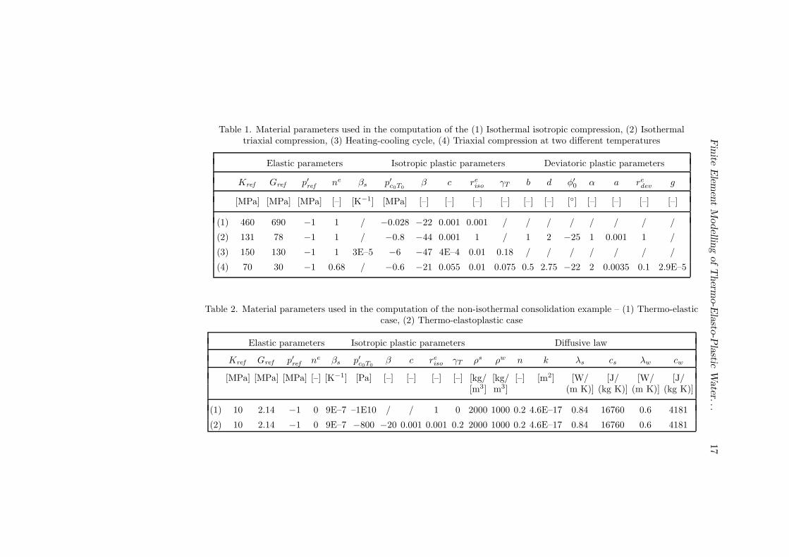
Table 1. Material parameters used in the computation of the (1) Isothermal isotropic compression, (2) Isothermaltriaxial compression, (3) Heating-cooling cycle, (4) Triaxial compression at two different temperatures

Elastic parameters Isotropic plastic parameters Deviatoric plastic parameters

Kref Gref p′ref ne βs p′c0T0

β c re

iso γT b d φ′

0α a re

dev g

[MPa] [MPa] [MPa] [–] [K−1] [MPa] [–] [–] [–] [–] [–] [–] [◦] [–] [–] [–] [–]

(1) 460 690 −1 1 / −0.028 −22 0.001 0.001 / / / / / / / /

(2) 131 78 −1 1 / −0.8 −44 0.001 1 / 1 2 −25 1 0.001 1 /

(3) 150 130 −1 1 3E–5 −6 −47 4E–4 0.01 0.18 / / / / / / /

(4) 70 30 −1 0.68 / −0.6 −21 0.055 0.01 0.075 0.5 2.75 −22 2 0.0035 0.1 2.9E–5

Table 2. Material parameters used in the computation of the non-isothermal consolidation example – (1) Thermo-elasticcase, (2) Thermo-elastoplastic case

Elastic parameters Isotropic plastic parameters Diffusive law

Kref Gref p′ref ne βs p′c0T0

β c re

iso γT ρs ρw n k λs cs λw cw

[MPa] [MPa] [MPa] [–] [K−1] [Pa] [–] [–] [–] [–] [kg/ [kg/ [–] [m2] [W/ [J/ [W/ [J/[m3] m3] (m K)] (kg K)] (m K)] (kg K)]

(1) 10 2.14 −1 0 9E–7 –1E10 / / 1 0 2000 1000 0.2 4.6E–17 0.84 16760 0.6 4181

(2) 10 2.14 −1 0 9E–7 −800 −20 0.001 0.001 0.2 2000 1000 0.2 4.6E–17 0.84 16760 0.6 4181


is of -6.0 MPa, -3.0 MPa and −1.0 MPa for OCR = 1; 2; 6, respectively.The comparison between the experimental and the finite element results

shows a very good agreement, as it can be seen in Fig. 4. This specific responseof soil depending on the stress state is very representative of thermo-plasticeffects, as already mentioned in Section 3.

Fig. 4. Heating-cooling at differentOCR: Comparison between the exper-imental [17] and the finite element re-

sults

Fig. 5. Simulation of triaxial sheartests under different confining pressures(p′

c= −600 kPa). Circle (square)

points: Experimental results at T =22 ◦C (T = 90 ◦C) [18]. Thin (thick)lines: numerical simulations at T =

22 ◦C (T = 90 ◦C)

The second set of experiments consists of triaxial tests on kaolin clayat two different temperatures (22 ◦C and 90 ◦C) and under different OCR [18].The cases of OCR = 1, 1.5 and 3 have been simulated at both temperatures.The comparison between the experimental and finite element results are de-picted in Fig. 5 and reveal a good capability of the ACMEG-T model im-plemented in the COMES-GEO code to describe the thermal effects on thedeviatoric response of soil, as observed experimentally. In particular, equation(6) coupled with equations (7) and (10) clearly shows that temperature inducesa change in the deviatoric yield limit, through the modification of preconsol-idation pressure and friction angle, and so modifies the stress-strain responseof soil when temperature changes.

6.2. Boundary value problem

The following example aims to validate the finite element formulation


solving an initial boundary value problem. It deals with the simulation of anon-isothermal fully saturated consolidation problem, for which the numericalsolution of the linear thermo-mechanical problem is known [15].

A column of 7 m height and 2 m width is subjected to an externalsurface compressive load of 1.0 kPa and to a surface temperature jump of 50K above the initial ambient temperature of 293.15 K. The material is initiallywater saturated. The upper surface is drained (pw = 0 Pa); the lateral andthe bottom surfaces are insulated. Horizontal displacements are constrainedalong the vertical boundaries and vertical displacements are constrained at thebottom surface. The column is discretized by nine eight-node isoparametricelements (Fig. 6). Furthermore, 3 × 3 Gauss integration points are used. Thematerial parameters used in the computation are listed in Table 2. Gravityforces are taken into account. Plane strain conditions are assumed.

Fig. 6. Spatial discretisation and boundary conditions for the non-isothermalconsolidation example

The case studied in [15], which assumed constant Young modulus (E =6.0 MPa) and Poisson ratio (ν = 0.4) and constant cubic thermal expansioncoefficient, is used as validation example. To this aim, the results of [15] aspublished in [4] and labelled “Aboustit et al.” in the Figs 7 and 8, are used tocompare the solution obtained with the finite element formulation proposed inthis paper and labelled “ACMEG-T”. The time histories for the water pres-sure (Fig. 7(a)), the temperature (Fig. 7(b)) and the vertical displacement(Fig. 7(c)) of several nodes of the mesh show the coincidence of the two solu-tions. The linear behaviour of the thermo-mechanical problem adopting the


Fig. 7. Simulation of non-isothermal fully saturated consolidation problem usinglinear thermo-elasticity and comparison with results of [4]. Evolution of pore water

pressure (a), temperature (b) and vertical displacement (c)


Fig. 8. Simulation of non-isothermal fully saturated consolidation problem usingthermo-elastoplasticity and comparison with results of [4]. Evolution of pore water

pressure (a), temperature (b) and vertical displacement (c)


ACMEG-T model is obtained by using the mechanical moduli independent ofthe stress state (ne = 0).

As shown all along the present paper, soils are often subject to irre-versible processes induced by thermal effect. In this context, the last simulationextends the problem of Fig. 6 towards thermo-elastoplastic analysis. The ma-terial parameters are listed in Table 2, where it can be observed that the linearelasticity is kept for comparison with the previous simulation; thermo-plasticityis introduced by reducing the preconsolidation pressure to get a mechanical andthermal hardening when loaded to 1 kPa and introducing the decrease of theisotropic yield surface with temperature.

The comparison between the elastic and the elasto-plastic solutionshows that the inclusion of the plasticity effects delays the dissipation of porewater pressure in time (Fig. 8(a)), because of the reduced thermo-plasticstiffness of the solid skeleton with respect to the elastic one. Moreover, thepredicted water pressures at the same time station are therefore higher thanthose from the elastic analysis.

Temperature evolution is almost not modified with respect to the pre-vious simulation, as it can be observed in Fig. 8(b). Indeed, because parame-ters of thermal conduction and convection are almost independent of porositychanges, at least for this range of volumetric strain, equation (3) remains al-most unaffected by mechanical change. On the contrary, the time history forthe vertical displacements appears to be strongly affected by thermo-plasticbehaviour of the solid skeleton. In particular, an increase of two order ofmagnitude for the vertical displacements is observed (Fig. 8(c)), that makesnegligible the thermal component that can be observed in Fig. 7(c).

7. Conclusions

A coupled finite element formulation for thermo-elastoplastic water sat-urated geomaterials based on Porous Media Mechanics was presented. To thisend, the ACMEG-T thermo-plastic constitutive model for saturated soils hasbeen implemented in the finite element code COMES-GEO for the analysis ofnon-isothermal elastoplastic multiphase solid porous materials.

Validation of the implemented model was made by selected comparisonbetween model simulation and experimental results for different combinationsof thermo-hydro-mechanical loading paths. A case of non-isothermal elastic orelasto-plastic consolidation was solved.

The model has been obtained as a result of a research in progress onthe thermo-hydro-mechanical modelling of multiphase geomaterials undergoing


inelastic strains. The validation case addressed in this paper remains verysimple but clearly points out that with a sufficiently general thermo-hydro-mechanical model, the main THM couplings occurring in fine soils may bereproduced in a relevant manner. In particular, thermo-elastoplastic effectscoupled with transient water and heat flow can be numerically analysed. Thatconstitutes a powerful tool to address many geoenvironmental problems.

REFEREN CES

[1] Laloui, L., C. Cekerevac. Thermo-Plasticity of Clays: An Isotropic YieldMechanism. Computers and Geotechnics, 30 (2003), 649–660.

[2] Laloui, L., C. Cekerevac, B. Francois. Constitutive Modelling of theThermo-Plastic Behaviour of Soils. Revue Europeenne de Genie Civil, 9 (2005),No. 5–6, 635–650.

[3] Sanavia, L., F. Pesavento, B. A. Schrefler. Finite Element Analysis ofNon-isothermal Multiphase Geomaterials with Application to Strain Localiza-tion Simulation. Computational Mechanics, 37 (2006), No. 4, 331–348.

[4] Lewis, R. W., B. A. Schrefler. The Finite Element Method in the Static andDynamic Deformation and Consolidation of Porous Media, J. Wiley, Chichester,1998.

[5] Gawin, D., B. A. Schrefler. Thermo-Hydro-Mechanical Analysis of PartiallySaturated Porous Materials. Engineering Computations, 13 (1996), No. 7, 113–143.

[6] Schrefler, B. A. Mechanics and Thermodynamics of Saturated-UnsaturatedPorous Materials and Quantitative Solutions. Applied Mechanics Review, 55

(2002), No. 4, 351–388.

[7] Hassanizadeh, M., W. G. Gray. General Conservation Equations for Multi-Phase System: 1. Averaging Technique. Adv. Water Res., 2 (1979), 131–144.

[8] Schrefler, B. A., L. Sanavia. Coupling Equations for Water Saturated andPartially Saturated Geomaterials. Revue Francaise de Genie Civil, 6 (2002),975–990.

[9] Gawin, D., L. Sanavia. Modelling of Cavitation and Rapid Water Desatura-tion of Porous Media Considering Effects of Dissolved Air. Transport in Porous

Media (Accepted).

[10] Laloui, L., B. Francois. ACMEG-T: A Comprehensive Soil Thermo-Plasticity Model. (Submitted).

[11] Hujeux, J. C. Une loi de comportement pour le chargement cyclique des sols,In: Genie Parasismique. Les editions de l’E.N.P.C, Paris, 1985, 287–302.

[12] Prager, W. Non-Isothermal Plastic Deformation. Koninkklijk-Nederland

Akademie Van Wetenschappen Te Amsterdam – Proceedings of the Section of

Sciences – B, 61 (1958), 176–182.


[13] Rizzi, E., G. Maier, K. Willam. On Failure Indicators in Multi-DissipativeMaterials. International Journal of Solids and Structures, 33 (1996), No. 20–22,3187–3214.

[14] Simo, J. C., T. J. R. Hughes. Computational Inelasticity, Springer, NewYork, 1998.

[15] Aboustit, B. L., S. H. Advani, J. K Lee. Variational Principles and Fi-nite Element Simulations for Thermo-Elastic Consolidation. Int. J. Num. Anal.

Meth. Geomech., 9 (1985), 49–69.

[16] Jamin, F. Contribution a l’etude du transport de matiere et de la rheologiedans les sols non satures a differentes temperatures, PhD Thesis, UniversiteMontpellier 2, 2003.

[17] Baldi, G., T. Hueckel, A. Peano, R. Pellegrini. Developments in Mod-elling of Thermo-Hydro-Geomechanical Behaviour of Boom Clay and Clay-Based Buffer Materials, Report: 13365/2 EN, Commission of the EuropeanCommunities, 1991.

[18] Cekerevac,C., L. Laloui. Experimental Study of the Thermal Effects onthe Mechanical Behaviour of a Clay. International Journal of Numerical and

Analytical Methods in Geomechanics, 28 (2004), 209–228.

FINITE ELEMENT MODELLING OF THERMO … words: thermo-elastoplasticity, water saturated porous...

Documents

Transcript of FINITE ELEMENT MODELLING OF THERMO … words: thermo-elastoplasticity, water saturated porous...