Finite Element Methods for the Simulation of ... · PDF fileWeierstrass Institute for Applied...
204
Weierstrass Institute for Applied Analysis and Stochastics Finite Element Methods for the Simulation of Incompressible Flows Volker John Mohrenstrasse 39 · 10117 Berlin · Germany · Tel. +49 30 20372 0 · www.wias-berlin.de · Course at Universidad Autonoma de Madrid, 27.02. – 02.03.2012
-
Upload
nguyendien -
Category
Documents
-
view
220 -
download
1
Transcript of Finite Element Methods for the Simulation of ... · PDF fileWeierstrass Institute for Applied...

Weierstrass Institute forApplied Analysis and Stochastics
Finite Element Methods for the Simulation ofIncompressible Flows
Volker John
Mohrenstrasse 39 · 10117 Berlin · Germany · Tel. +49 30 20372 0 · www.wias-berlin.de · Course at Universidad Autonoma de Madrid, 27.02. – 02.03.2012
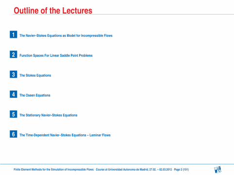
Outline of the Lectures
1 The Navier–Stokes Equations as Model for Incompressible Flows
2 Function Spaces For Linear Saddle Point Problems
3 The Stokes Equations
4 The Oseen Equations
5 The Stationary Navier–Stokes Equations
6 The Time-Dependent Navier–Stokes Equations – Laminar Flows
Finite Element Methods for the Simulation of Incompressible Flows · Course at Universidad Autonoma de Madrid, 27.02. – 02.03.2012 · Page 2 (151)

1 A Model for Incompressible Flows
• conservation laws conservation of linear momentum conservation of mass
• flow variables ρ(t,x) : density [kg/m3]
v(t,x) : velocity [m/s] P(t,x) : pressure [N/m2]
assumed to be sufficiently smooth in• Ω⊂ R3
• [0,T ]
Finite Element Methods for the Simulation of Incompressible Flows · Course at Universidad Autonoma de Madrid, 27.02. – 02.03.2012 · Page 3 (151)
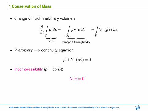
1 Conservation of Mass
• change of fluid in arbitrary volume V
− ∂
∂ t
∫V
ρ dx
︸ ︷︷ ︸mass
=∫
∂V
ρv ·n ds
︸ ︷︷ ︸transport through bdry
=∫V
∇ · (ρv) dx
• V arbitrary =⇒ continuity equation
ρt +∇ · (ρv) = 0
• incompressibility (ρ = const)
∇ ·v = 0
Finite Element Methods for the Simulation of Incompressible Flows · Course at Universidad Autonoma de Madrid, 27.02. – 02.03.2012 · Page 4 (151)
1 Newton’s Second Law of Motion
• Newton’s second law of motion
net force = mass × acceleration
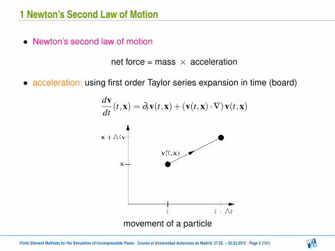
• acceleration: using first order Taylor series expansion in time (board)
dvdt
(t,x) = ∂tv(t,x)+(v(t,x) ·∇)v(t,x)
movement of a particle
Finite Element Methods for the Simulation of Incompressible Flows · Course at Universidad Autonoma de Madrid, 27.02. – 02.03.2012 · Page 5 (151)
1 Newton’s Second Law of Motion
• Newton’s second law of motion
net force = mass × acceleration
• acceleration: using first order Taylor series expansion in time (board)
dvdt
(t,x) = ∂tv(t,x)+(v(t,x) ·∇)v(t,x)
movement of a particle
Finite Element Methods for the Simulation of Incompressible Flows · Course at Universidad Autonoma de Madrid, 27.02. – 02.03.2012 · Page 5 (151)

1 Newton’s Second Law of Motion
• acting forces on an arbitrary volume V :sum of external (body) forces gravity
and internal (molecular) forces pressure viscous drag that a ’fluid element’ exerts on the ’adjacent element’ contact forces: act only on surface of ’fluid element’∫
VF(t,x) dx+
∫∂V
t(t,s) ds
t [N/m2] – Cauchy stress vector
• principle of Cauchy: internal contact forces depend (geometrically) onlyon the orientation of the surface
t = t(n)
n – unit normal vector of the surface pointing outwards of V
Finite Element Methods for the Simulation of Incompressible Flows · Course at Universidad Autonoma de Madrid, 27.02. – 02.03.2012 · Page 6 (151)

1 Newton’s Second Law of Motion
• acting forces on an arbitrary volume V :sum of external (body) forces gravity
and internal (molecular) forces pressure viscous drag that a ’fluid element’ exerts on the ’adjacent element’ contact forces: act only on surface of ’fluid element’∫
VF(t,x) dx+
∫∂V
t(t,s) ds
t [N/m2] – Cauchy stress vector• principle of Cauchy: internal contact forces depend (geometrically) only
on the orientation of the surface
t = t(n)
n – unit normal vector of the surface pointing outwards of V
Finite Element Methods for the Simulation of Incompressible Flows · Course at Universidad Autonoma de Madrid, 27.02. – 02.03.2012 · Page 6 (151)
1 Newton’s Second Law of Motion
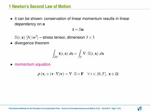
• it can be shown: conservation of linear momentum results in lineardependency on n
t = Sn
S(t,x) [N/m2] – stress tensor, dimension 3×3• divergence theorem ∫
∂Vt(t,s) ds =
∫V
∇ ·S(t,x) dx
• momentum equation
ρ (vt +(v ·∇)v) = ∇ ·S+F ∀ t ∈ (0,T ], x ∈Ω
Finite Element Methods for the Simulation of Incompressible Flows · Course at Universidad Autonoma de Madrid, 27.02. – 02.03.2012 · Page 7 (151)
1 Newton’s Second Law of Motion
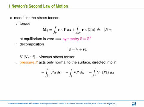
• model for the stress tensor torque
M0 =∫
Vr×F dx+
∫∂V
r× (Sn) ds [N m]
at equilibrium is zero =⇒ symmetry S= ST
decompositionS= V+PI
V [N/m2] – viscous stress tensor pressure P acts only normal to the surface, directed into V
−∫
∂VPn ds =−
∫V
∇P dx =−∫
V∇ · (PI) dx
Finite Element Methods for the Simulation of Incompressible Flows · Course at Universidad Autonoma de Madrid, 27.02. – 02.03.2012 · Page 8 (151)
1 Newton’s Second Law of Motion
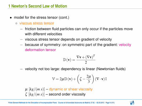
• model for the stress tensor (cont.) viscous stress tensor− friction between fluid particles can only occur if the particles move
with different velocities− viscous stress tensor depends on gradient of velocity− because of symmetry: on symmetric part of the gradient: velocity
deformation tensor
D(v) =∇v+(∇v)T
2
− velocity not too large: dependency is linear (Newtonian fluids)
V= 2µD(v)+(
ζ − 2µ
3
)(∇ ·v)I
µ [kg/(m s)] – dynamic or shear viscosityζ [kg/(m s)] – second order viscosity
Finite Element Methods for the Simulation of Incompressible Flows · Course at Universidad Autonoma de Madrid, 27.02. – 02.03.2012 · Page 9 (151)
1 Navier–Stokes Equations
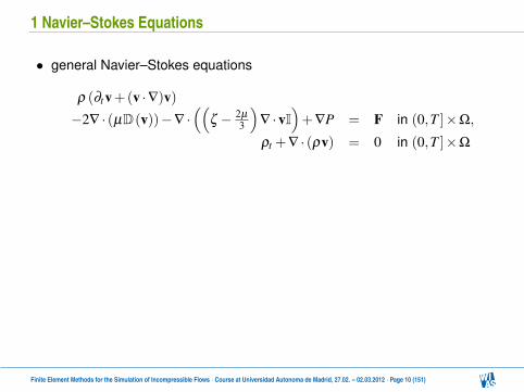
• general Navier–Stokes equations
ρ (∂tv+(v ·∇)v)−2∇ · (µD(v))−∇ ·
((ζ − 2µ
3
)∇ ·vI
)+∇P = F in (0,T ]×Ω,
ρt +∇ · (ρv) = 0 in (0,T ]×Ω
• incompressible flows: incompressible Navier–Stokes equations
∂tv−2ν∇ ·D(v)+(v ·∇)v+∇Pρ0
=Fρ0
in (0,T ]×Ω,
∇ ·v = 0 in (0,T ]×Ω
Finite Element Methods for the Simulation of Incompressible Flows · Course at Universidad Autonoma de Madrid, 27.02. – 02.03.2012 · Page 10 (151)

1 Navier–Stokes Equations
• general Navier–Stokes equations
ρ (∂tv+(v ·∇)v)−2∇ · (µD(v))−∇ ·
((ζ − 2µ
3
)∇ ·vI
)+∇P = F in (0,T ]×Ω,
ρt +∇ · (ρv) = 0 in (0,T ]×Ω
• incompressible flows: incompressible Navier–Stokes equations
∂tv−2ν∇ ·D(v)+(v ·∇)v+∇Pρ0
=Fρ0
in (0,T ]×Ω,
∇ ·v = 0 in (0,T ]×Ω
Finite Element Methods for the Simulation of Incompressible Flows · Course at Universidad Autonoma de Madrid, 27.02. – 02.03.2012 · Page 10 (151)
1 Navier–Stokes Equations
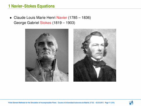
• Claude Louis Marie Henri Navier (1785 – 1836)George Gabriel Stokes (1819 – 1903)
Finite Element Methods for the Simulation of Incompressible Flows · Course at Universidad Autonoma de Madrid, 27.02. – 02.03.2012 · Page 11 (151)
1 Dimensionless Incompressible Navier–Stokes Equations
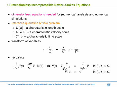
• dimensionless equations needed for (numerical) analysis and numericalsimulations
• reference quantities of flow problem L [m] – a characteristic length scale U [m/s] – a characteristic velocity scale T ∗ [s] – a characteristic time scale
• transform of variables
x =x′
L, u =
vU, t =
t ′
T ∗
• rescaling
LUT ∗
∂tu−2ν
UL∇ ·D(u)+(u ·∇)u+∇
Pρ0U2 =
Lρ0U2 F in (0,T ]×Ω,
∇ ·u = 0 in (0,T ]×Ω,
Finite Element Methods for the Simulation of Incompressible Flows · Course at Universidad Autonoma de Madrid, 27.02. – 02.03.2012 · Page 12 (151)
1 Dimensionless Incompressible Navier–Stokes Equations
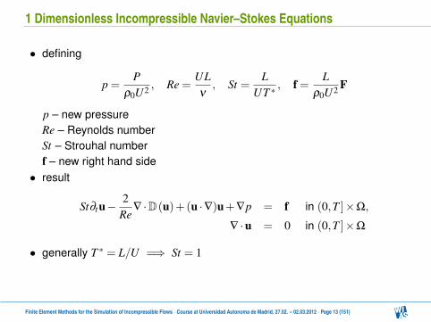
• defining
p =P
ρ0U2 , Re =ULν
, St =L
UT ∗, f =
Lρ0U2 F
p – new pressureRe – Reynolds numberSt – Strouhal numberf – new right hand side
• result
St∂tu−2
Re∇ ·D(u)+(u ·∇)u+∇p = f in (0,T ]×Ω,
∇ ·u = 0 in (0,T ]×Ω
• generally T ∗ = L/U =⇒ St = 1
Finite Element Methods for the Simulation of Incompressible Flows · Course at Universidad Autonoma de Madrid, 27.02. – 02.03.2012 · Page 13 (151)
1 Dimensionless Incompressible Navier–Stokes Equations
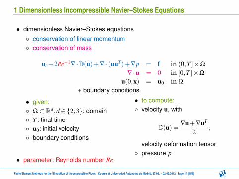
• dimensionless Navier–Stokes equations conservation of linear momentum conservation of mass
ut −2Re−1∇ ·D(u)+∇ · (uuT )+∇p = f in (0,T ]×Ω
∇ ·u = 0 in [0,T ]×Ω
u(0,x) = u0 in Ω
+ boundary conditions
• given: Ω⊂ Rd ,d ∈ 2,3: domain T : final time u0: initial velocity boundary conditions
• to compute: velocity u, with
D(u) =∇u+∇uT
2,
velocity deformation tensor pressure p
• parameter: Reynolds number Re
Finite Element Methods for the Simulation of Incompressible Flows · Course at Universidad Autonoma de Madrid, 27.02. – 02.03.2012 · Page 14 (151)

1 The Reynolds Number
• Reynolds number
Re =LUν
=convective forces
viscous forces
Osborne Reynolds (1842 – 1912)• rough classification of flows: Re small: steady-state flow field (if data do not depend on time) Re larger: laminar time-dependent flow field Re very large: turbulent flows
Finite Element Methods for the Simulation of Incompressible Flows · Course at Universidad Autonoma de Madrid, 27.02. – 02.03.2012 · Page 15 (151)

1 Dimensionless Incompressible Navier–Stokes Equations
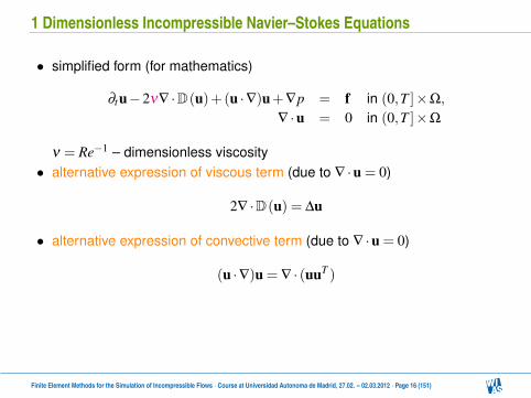
• simplified form (for mathematics)
∂tu−2ν∇ ·D(u)+(u ·∇)u+∇p = f in (0,T ]×Ω,
∇ ·u = 0 in (0,T ]×Ω
ν = Re−1 – dimensionless viscosity
• alternative expression of viscous term (due to ∇ ·u = 0)
2∇ ·D(u) = ∆u
• alternative expression of convective term (due to ∇ ·u = 0)
(u ·∇)u = ∇ · (uuT )
Finite Element Methods for the Simulation of Incompressible Flows · Course at Universidad Autonoma de Madrid, 27.02. – 02.03.2012 · Page 16 (151)
1 Dimensionless Incompressible Navier–Stokes Equations
• simplified form (for mathematics)
∂tu−2ν∇ ·D(u)+(u ·∇)u+∇p = f in (0,T ]×Ω,
∇ ·u = 0 in (0,T ]×Ω
ν = Re−1 – dimensionless viscosity• alternative expression of viscous term (due to ∇ ·u = 0)
2∇ ·D(u) = ∆u
• alternative expression of convective term (due to ∇ ·u = 0)
(u ·∇)u = ∇ · (uuT )
Finite Element Methods for the Simulation of Incompressible Flows · Course at Universidad Autonoma de Madrid, 27.02. – 02.03.2012 · Page 16 (151)

1 Incompressible Navier–Stokes Equations
• special cases steady-state Navier–Stokes equations: stationary flow fields
−ν∆u+(u ·∇)u+∇p = f in Ω
∇ ·u = 0 in Ω
Oseen equations: convection field known (only for analysis)
−ν∆u+(u0 ·∇)u+∇p+ cu = f in Ω
∇ ·u = 0 in Ω
Stokes equations: no convection
−∆u+∇p = f in Ω
∇ ·u = 0 in Ω
Finite Element Methods for the Simulation of Incompressible Flows · Course at Universidad Autonoma de Madrid, 27.02. – 02.03.2012 · Page 17 (151)

1 Incompressible Navier–Stokes Equations
• boundary conditions Dirichlet boundary conditions (inflows)
u(t,x) = g(t,x) in (0,T ]×Γdiri ⊂ Γ
g(t,x) = 0 – no slip boundary condition (walls)
u(t,x) = 0 ⇐⇒ u(t,x) ·n = 0, u(t,x) · t1 = 0, u(t,x) · t2 = 0
no penetration, no slip
free slip boundary condition (e.g. symmetry planes)
u ·n = g in (0,T ]×Γslip ⊂ Γ,
nTStk = 0 in (0,T ]×Γslip, 1≤ k ≤ d−1
Finite Element Methods for the Simulation of Incompressible Flows · Course at Universidad Autonoma de Madrid, 27.02. – 02.03.2012 · Page 18 (151)

1 Incompressible Navier–Stokes Equations
• boundary conditions Dirichlet boundary conditions (inflows)
u(t,x) = g(t,x) in (0,T ]×Γdiri ⊂ Γ
g(t,x) = 0 – no slip boundary condition (walls)
u(t,x) = 0 ⇐⇒ u(t,x) ·n = 0, u(t,x) · t1 = 0, u(t,x) · t2 = 0
no penetration, no slip free slip boundary condition (e.g. symmetry planes)
u ·n = g in (0,T ]×Γslip ⊂ Γ,
nTStk = 0 in (0,T ]×Γslip, 1≤ k ≤ d−1
Finite Element Methods for the Simulation of Incompressible Flows · Course at Universidad Autonoma de Madrid, 27.02. – 02.03.2012 · Page 18 (151)
1 Incompressible Navier–Stokes Equations
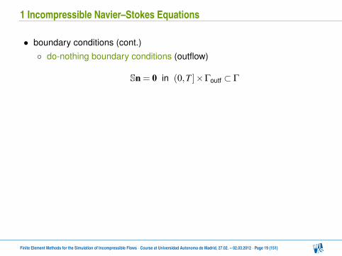
• boundary conditions (cont.) do-nothing boundary conditions (outflow)
Sn = 0 in (0,T ]×Γoutf ⊂ Γ
periodic boundary conditions (only for analysis, Ω = (0, l)d)
u(t,x+ lei) = u(t,x) ∀ (t,x) ∈ (0,T ]×Γ
Finite Element Methods for the Simulation of Incompressible Flows · Course at Universidad Autonoma de Madrid, 27.02. – 02.03.2012 · Page 19 (151)
1 Incompressible Navier–Stokes Equations
• difficulties for mathematical analysis and numerical simulations coupling of velocity and pressure nonlinearity of the convective term the convective term dominates the viscous term, i.e. ν is small
Finite Element Methods for the Simulation of Incompressible Flows · Course at Universidad Autonoma de Madrid, 27.02. – 02.03.2012 · Page 20 (151)
2 Linear Saddle Point Problems
• motivation iterative solution of Navier–Stokes equations leads to linear system of
equations linear system have special form: saddle point problem sufficient and necessary condition on unique solvability needed can be derived in abstract form, see [1]
[1] Girault, Raviart: Finite Element Methods for Navier-Stokes Equations 1986
Finite Element Methods for the Simulation of Incompressible Flows · Course at Universidad Autonoma de Madrid, 27.02. – 02.03.2012 · Page 21 (151)
2 Linear Saddle Point Problems
• spaces: V,Q – real Hilbert spaces• bilinear forms:
a(·, ·) : V ×V → R, b(·, ·) : V ×Q→ R
• linear problem: Find (u, p) ∈V ×Q such that for given ( f ,r) ∈V ′×Q′
a(u,v)+b(v, p) = 〈 f ,v〉V ′,V ∀ v ∈V,b(u,q) = 〈r,q〉Q′,Q ∀ q ∈ Q
• conditions on the spaces and bilinear forms necessary
Finite Element Methods for the Simulation of Incompressible Flows · Course at Universidad Autonoma de Madrid, 27.02. – 02.03.2012 · Page 22 (151)
2 Linear Saddle Point Problems
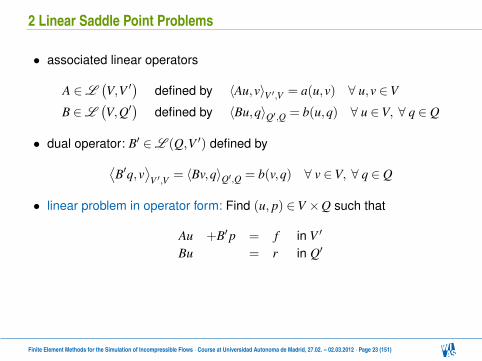
• associated linear operators
A ∈L(V,V ′
)defined by 〈Au,v〉V ′,V = a(u,v) ∀ u,v ∈V
B ∈L(V,Q′
)defined by 〈Bu,q〉Q′,Q = b(u,q) ∀ u ∈V, ∀ q ∈ Q
• dual operator: B′ ∈L (Q,V ′) defined by⟨B′q,v
⟩V ′,V = 〈Bv,q〉Q′,Q = b(v,q) ∀ v ∈V, ∀ q ∈ Q
• linear problem in operator form: Find (u, p) ∈V ×Q such that
Au +B′p = f in V ′
Bu = r in Q′
Finite Element Methods for the Simulation of Incompressible Flows · Course at Universidad Autonoma de Madrid, 27.02. – 02.03.2012 · Page 23 (151)
2 The Inf-Sup Condition – Bilinear Form b(·, ·)
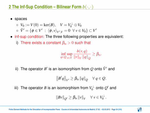
• spaces V0 :=V (0) = ker(B), V =V⊥0 ⊕V0
V ′ = φ ∈V ′ : 〈φ ,v〉V ′,V = 0 ∀ v ∈V0 ⊂V ′
• inf-sup condition: The three following properties are equivalent:i) There exists a constant βis > 0 such that
infq∈Q
supv∈V
b(v,q)‖v‖V ‖q‖Q
≥ βis.
ii) The operator B′ is an isomorphism from Q onto V ′ and∥∥B′q∥∥
V ′ ≥ βis ‖q‖Q ∀ q ∈ Q.
iii) The operator B is an isomorphism from V⊥0 onto Q′ and
‖Bv‖Q′ ≥ βis ‖v‖V ∀ v ∈V⊥0 .
Finite Element Methods for the Simulation of Incompressible Flows · Course at Universidad Autonoma de Madrid, 27.02. – 02.03.2012 · Page 24 (151)

2 The Inf-Sup Condition – Bilinear Form b(·, ·)
• independently derived in [1,2]: Babuška–Brezzi condition• sometimes: Ladyzhenskaya–Babuška–Brezzi condition, LBB condition• it follows:
V (r) = v ∈V : Bv = r
is not empty for all r ∈ Q′
[1] Babuška: Numer. Math. 20, 179–192, 1973
[2] Brezzi: Rev. Française Automat. Informat. Recherche Opérationnelle Sér. Rouge 8, 129–151, 1974
Finite Element Methods for the Simulation of Incompressible Flows · Course at Universidad Autonoma de Madrid, 27.02. – 02.03.2012 · Page 25 (151)

2 Unique Solution of Linear Saddle Point Problem
• sufficient and necessary conditions for unique solution of saddle pointproblem can be formulated with projection operator, see literature
• sufficient conditions a(·, ·) is V0-elliptic, i.e., there is a constant α > 0 such that
a(v,v)≥ α ‖v‖2V ∀ v ∈V0
b(·, ·) satisfies inf-sup condition
Finite Element Methods for the Simulation of Incompressible Flows · Course at Universidad Autonoma de Madrid, 27.02. – 02.03.2012 · Page 26 (151)
2 Continuous Incompressible Flow Problems
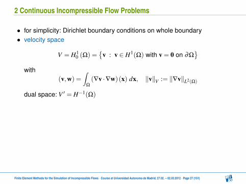
• for simplicity: Dirichlet boundary conditions on whole boundary• velocity space
V = H10 (Ω) =
v : v ∈ H1(Ω) with v = 0 on ∂Ω
with
(v,w) =∫
Ω
(∇v ·∇w)(x) dx, ‖v‖V := ‖∇v‖L2(Ω)
dual space: V ′ = H−1(Ω)
• pressure space
Q = L20 (Ω) =
q : q ∈ L2(Ω) with
∫Ω
q(x) dx = 0
with(q,r) =
∫Ω
(qr)(x) dx, ‖q‖Q = ‖q‖L2(Ω)
• dual space: Q′ = Q
Finite Element Methods for the Simulation of Incompressible Flows · Course at Universidad Autonoma de Madrid, 27.02. – 02.03.2012 · Page 27 (151)

2 Continuous Incompressible Flow Problems
• bilinear form for coupling velocity and pressure
b(v,q) =−∫
Ω
q∇ ·v dx =−(∇ ·v,q) v ∈V, q ∈ Q
• divergence operator
div : V → range(div), v 7→ ∇ ·v
• it can be shown: range(div) = Q′
• associated linear operator: negative divergence operator
B ∈L (V,Q′), B =−div
Finite Element Methods for the Simulation of Incompressible Flows · Course at Universidad Autonoma de Madrid, 27.02. – 02.03.2012 · Page 28 (151)
2 Continuous Incompressible Flow Problems
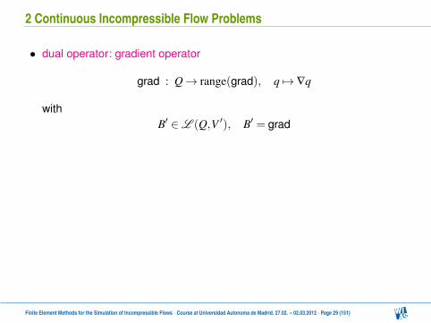
• dual operator: gradient operator
grad : Q→ range(grad), q 7→ ∇q
withB′ ∈L (Q,V ′), B′ = grad
• kernel of B: space of weakly divergence-free functions
V0 =Vdiv = v ∈V : (∇ ·v,q) = 0 ∀ q ∈ Q
Finite Element Methods for the Simulation of Incompressible Flows · Course at Universidad Autonoma de Madrid, 27.02. – 02.03.2012 · Page 29 (151)
2 Continuous Incompressible Flow Problems
• dual operator: gradient operator
grad : Q→ range(grad), q 7→ ∇q
withB′ ∈L (Q,V ′), B′ = grad
• kernel of B: space of weakly divergence-free functions
V0 =Vdiv = v ∈V : (∇ ·v,q) = 0 ∀ q ∈ Q
Finite Element Methods for the Simulation of Incompressible Flows · Course at Universidad Autonoma de Madrid, 27.02. – 02.03.2012 · Page 29 (151)

2 Continuous Incompressible Flow Problems
• estimating divergence by gradient
‖∇ ·v‖L2(Ω) ≤√
d ‖∇v‖L2(Ω) ∀ v ∈ H1(Ω)
proof: board estimate is sharp
• boundedness and continuity of b(·, ·)
|b(v,q)| ≤√
d ‖v‖V ‖q‖Q
proof: board
Finite Element Methods for the Simulation of Incompressible Flows · Course at Universidad Autonoma de Madrid, 27.02. – 02.03.2012 · Page 30 (151)
2 Continuous Incompressible Flow Problems
• one can show: div is an isomorphism from V⊥div onto Q• corollary: each pressure is the divergence of a velocity field:
for each q ∈ Q there is a unique v ∈V⊥div ⊂V such that
∇ ·v = q and ‖q‖Q ≤√
d ‖v‖V , ‖v‖V ≤C‖q‖Q
with C independent of v and q proof: board
• V and Q fulfill the inf-sup condition, i.e. there is a βis > 0 such that
infq∈Q
supv∈V
(∇ ·v,q)‖v‖V
≥ βis
proof: board
Finite Element Methods for the Simulation of Incompressible Flows · Course at Universidad Autonoma de Madrid, 27.02. – 02.03.2012 · Page 31 (151)
2 Finite Element Spaces
• finite element spaces V h – finite element velocity space Qh – finite element pressure space V h/Qh – pair
• conforming finite element spaces: V h ⊂V and Qh ⊂ Q
• bilinear form bh : V h×Qh→ R
bh(
vh,qh)
:=− ∑K∈T h
(∇ ·vh,qh
)K
T h – triangulation of Ω
K ∈T h – mesh cells norm in V h ∥∥∥vh
∥∥∥V h
= ∑K∈T h
(∇vh,∇vh
)K
Finite Element Methods for the Simulation of Incompressible Flows · Course at Universidad Autonoma de Madrid, 27.02. – 02.03.2012 · Page 32 (151)
2 Finite Element Spaces
• finite element spaces V h – finite element velocity space Qh – finite element pressure space V h/Qh – pair
• conforming finite element spaces: V h ⊂V and Qh ⊂ Q• bilinear form bh : V h×Qh→ R
bh(
vh,qh)
:=− ∑K∈T h
(∇ ·vh,qh
)K
T h – triangulation of Ω
K ∈T h – mesh cells norm in V h ∥∥∥vh
∥∥∥V h
= ∑K∈T h
(∇vh,∇vh
)K
Finite Element Methods for the Simulation of Incompressible Flows · Course at Universidad Autonoma de Madrid, 27.02. – 02.03.2012 · Page 32 (151)
2 Finite Element Spaces
• space of discretely divergence-free functions
V hdiv =
vh ∈V h : bh
(vh,qh
)= 0 ∀ qh ∈ Qh
• generally V h
div 6⊂Vdiv
finite element velocities not weakly or pointwise divergence-free conservation of mass violated
• discrete inf-sup condition
infqh∈Qh
supvh∈V h
bh(vh,qh
)‖vh‖V h ‖qh‖L2(Ω)
≥ βhis > 0
not inherited from inf-sup condition fulfilled by V and Q discussion: board
Finite Element Methods for the Simulation of Incompressible Flows · Course at Universidad Autonoma de Madrid, 27.02. – 02.03.2012 · Page 33 (151)
2 Finite Element Spaces
• Interpolation estimate for V hdiv. Let v ∈Vdiv and let the discrete inf-sup
condition hold. Then
infvh∈V h
div
∥∥∥∇
(v−vh
)∥∥∥L2(Ω)
≤
(1+
√d
β his
)inf
wh∈V h
∥∥∥∇
(v−wh
)∥∥∥L2(Ω)
proof: board
Finite Element Methods for the Simulation of Incompressible Flows · Course at Universidad Autonoma de Madrid, 27.02. – 02.03.2012 · Page 34 (151)
2 Finite Elements
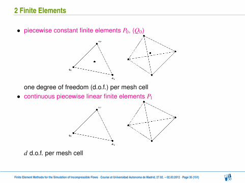
• piecewise constant finite elements P0, (Q0)
one degree of freedom (d.o.f.) per mesh cell• continuous piecewise linear finite elements P1
d d.o.f. per mesh cell
Finite Element Methods for the Simulation of Incompressible Flows · Course at Universidad Autonoma de Madrid, 27.02. – 02.03.2012 · Page 35 (151)

2 Finite Elements
• continuous piecewise quadratic finite elements P2
(d +1)(d +2)/2 d.o.f. per mesh cell• continuous piecewise bilinear finite elements Q1
2d d.o.f. per mesh cell• and so on for continuous finite elements of higher order
Finite Element Methods for the Simulation of Incompressible Flows · Course at Universidad Autonoma de Madrid, 27.02. – 02.03.2012 · Page 36 (151)
2 Finite Elements
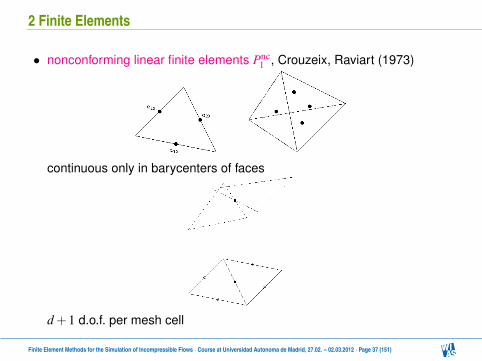
• nonconforming linear finite elements Pnc1 , Crouzeix, Raviart (1973)
continuous only in barycenters of faces
d +1 d.o.f. per mesh cell
Finite Element Methods for the Simulation of Incompressible Flows · Course at Universidad Autonoma de Madrid, 27.02. – 02.03.2012 · Page 37 (151)

2 Finite Elements
• rotated bilinear finite element Qrot1 , Rannacher, Turek (1992)
continuous only in barycenters of faces 2d d.o.f. per mesh cell
• discontinuous linear finite element Pdisc1
defined by integral nodal functionalse.g. ϕh ∈ Pdisc
1 if ϕh is linear on a mesh cell K (2d) and∫K
ϕh(x) dx = 0,
∫K
xϕh(x) dx = 1,
∫K
yϕh(x) dx = 0
d +1 d.o.f. per mesh cell
Finite Element Methods for the Simulation of Incompressible Flows · Course at Universidad Autonoma de Madrid, 27.02. – 02.03.2012 · Page 38 (151)

2 Finite Element Spaces
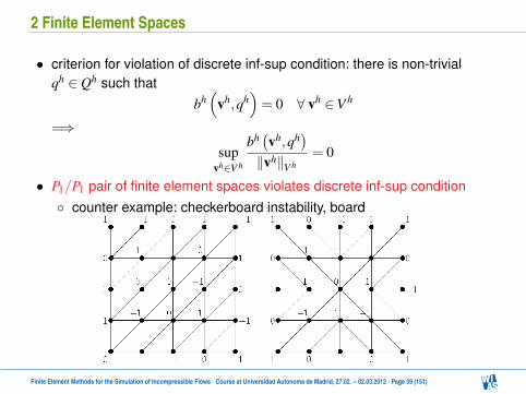
• criterion for violation of discrete inf-sup condition: there is non-trivialqh ∈ Qh such that
bh(
vh,qh)= 0 ∀ vh ∈V h
=⇒
supvh∈V h
bh(vh,qh
)‖vh‖V h
= 0
• P1/P1 pair of finite element spaces violates discrete inf-sup condition counter example: checkerboard instability, board
Finite Element Methods for the Simulation of Incompressible Flows · Course at Universidad Autonoma de Madrid, 27.02. – 02.03.2012 · Page 39 (151)
2 Finite Element Spaces
• other pairs which violated discrete inf-sup condition P1/P0
Q1/Q0
Pk/Pk, k ≥ 1 Qk/Qk, k ≥ 1 Pk/Pdisc
k−1 , k ≥ 2, on a special macro cell• summary: many easy to implement pairs violate discrete inf-sup condition different finite element spaces for velocity and pressure necessary
Finite Element Methods for the Simulation of Incompressible Flows · Course at Universidad Autonoma de Madrid, 27.02. – 02.03.2012 · Page 40 (151)
2 Finite Element Spaces
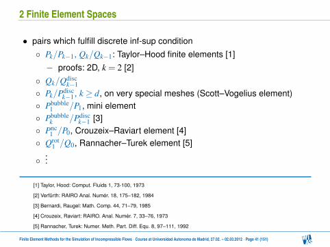
• pairs which fulfill discrete inf-sup condition Pk/Pk−1, Qk/Qk−1: Taylor–Hood finite elements [1]− proofs: 2D, k = 2 [2]
Qk/Qdisck−1
Pk/Pdisck−1 , k ≥ d, on very special meshes (Scott–Vogelius element)
Pbubble1 /P1, mini element
Pbubblek /Pdisc
k−1 [3] Pnc
1 /P0, Crouzeix–Raviart element [4] Qrot
1 /Q0, Rannacher–Turek element [5]
...
[1] Taylor, Hood: Comput. Fluids 1, 73-100, 1973
[2] Verfürth: RAIRO Anal. Numér. 18, 175–182, 1984
[3] Bernardi, Raugel: Math. Comp. 44, 71–79, 1985
[4] Crouzeix, Raviart: RAIRO. Anal. Numér. 7, 33–76, 1973
[5] Rannacher, Turek: Numer. Meth. Part. Diff. Equ. 8, 97–111, 1992
Finite Element Methods for the Simulation of Incompressible Flows · Course at Universidad Autonoma de Madrid, 27.02. – 02.03.2012 · Page 41 (151)
2 Finite Element Spaces
• techniques for proving the discrete inf-sup condition construction of Fortin operator [1] using projection to piecewise constant pressure [2] macroelement technique [3] survey in [4]
[1] Fortin: RAIRO Anal. Numér. 11, 341–354, 1977
[2] Brezzi, Bathe: Comput. Methods Appl. Mech. Engrg. 82, 27–57, 1990
[3] Stenberg: Math. Comput. 32, 9–23, 1984
[4] Boffi, Brezzi, Fortin: Lecture Notes in Mathematics 1939, Springer, 45–100, 2008
Finite Element Methods for the Simulation of Incompressible Flows · Course at Universidad Autonoma de Madrid, 27.02. – 02.03.2012 · Page 42 (151)
3 The Stokes Equations
• continuous equation
−∆u+∇p = f in Ω,
∇ ·u = 0 in Ω(1)
for simplicity: homogeneous Dirichlet boundary conditions• difficulty: coupling of velocity and pressure• properties linear form
−ν∆u+∇p = f in Ω,
∇ ·u = 0 in Ω
becomes (1) by rescaling with new pressure, right hand side
Finite Element Methods for the Simulation of Incompressible Flows · Course at Universidad Autonoma de Madrid, 27.02. – 02.03.2012 · Page 43 (151)
3 The Stokes Equations
• weak form: Find (u, p) ∈ H10 (Ω)×L2
0(Ω) such that
(∇u,∇v)− (∇ ·v, p) = 〈f,v〉H−1(Ω),H10 (Ω) ∀ v ∈ H1
0 (Ω),
−(∇ ·u,q) = 0 ∀ q ∈ L20(Ω)
• casting into abstract framework spaces
V = H10 (Ω), ‖·‖V = |·|H1(Ω) , Q = L2
0(Ω), ‖·‖Q = ‖·‖L2(Ω)
bilinear forms
a(u,v) = (∇u,∇v), b(v,q) =−(∇ ·v,q)
• equivalent formulation: Find (u, p) ∈V ×Q such that
a(u,v)+b(v, p)−b(u,q) = 〈f,v〉V ′,V ∀ (v,q) ∈V ×Q
Finite Element Methods for the Simulation of Incompressible Flows · Course at Universidad Autonoma de Madrid, 27.02. – 02.03.2012 · Page 44 (151)
3 The Stokes Equations
• Vdiv – space of weakly divergence-free functions• associated problem: Find u ∈Vdiv such that
(∇u,∇v) = 〈f,v〉V ′,V ∀ v ∈Vdiv
• existence and uniqueness of solution a(·, ·) is Vdiv-elliptic
a(v,v) = |v|2H1(Ω) ∀ v ∈V ⊃Vdiv
b(·, ·) satisfies inf-sup condition• stability of solution
‖∇u‖L2(Ω) ≤ ‖f‖H−1(Ω) , ‖p‖L2(Ω) ≤2
βis‖f‖H−1(Ω)
proof and discussion: board
Finite Element Methods for the Simulation of Incompressible Flows · Course at Universidad Autonoma de Madrid, 27.02. – 02.03.2012 · Page 45 (151)

3 The Stokes Equations
• Vdiv – space of weakly divergence-free functions• associated problem: Find u ∈Vdiv such that
(∇u,∇v) = 〈f,v〉V ′,V ∀ v ∈Vdiv
• existence and uniqueness of solution a(·, ·) is Vdiv-elliptic
a(v,v) = |v|2H1(Ω) ∀ v ∈V ⊃Vdiv
b(·, ·) satisfies inf-sup condition
• stability of solution
‖∇u‖L2(Ω) ≤ ‖f‖H−1(Ω) , ‖p‖L2(Ω) ≤2
βis‖f‖H−1(Ω)
proof and discussion: board
Finite Element Methods for the Simulation of Incompressible Flows · Course at Universidad Autonoma de Madrid, 27.02. – 02.03.2012 · Page 45 (151)
3 The Stokes Equations
• Vdiv – space of weakly divergence-free functions• associated problem: Find u ∈Vdiv such that
(∇u,∇v) = 〈f,v〉V ′,V ∀ v ∈Vdiv
• existence and uniqueness of solution a(·, ·) is Vdiv-elliptic
a(v,v) = |v|2H1(Ω) ∀ v ∈V ⊃Vdiv
b(·, ·) satisfies inf-sup condition• stability of solution
‖∇u‖L2(Ω) ≤ ‖f‖H−1(Ω) , ‖p‖L2(Ω) ≤2
βis‖f‖H−1(Ω)
proof and discussion: board
Finite Element Methods for the Simulation of Incompressible Flows · Course at Universidad Autonoma de Madrid, 27.02. – 02.03.2012 · Page 45 (151)
3 Finite Element Methods for the Stokes Equations
• finite element problem: Find (uh, ph) ∈V h×Qh such that
ah(uh,vh
)+bh
(vh, ph
)=
(f,vh
)∀ vh ∈V h,
bh(uh,qh
)= 0 ∀ qh ∈ Qh
with
ah(
vh,wh)= ∑
K∈T h
(∇vh,∇wh
)K, bh
(vh,qh
)=− ∑
K∈T h
(∇ ·vh,qh
)K
• only conforming inf-sup stable finite element spaces V h ⊂V and Qh ⊂ Q
infqh∈Qh
supvh∈V h
bh(vh,qh
)‖vh‖V h ‖qh‖L2(Ω)
≥ βhis > 0
Finite Element Methods for the Simulation of Incompressible Flows · Course at Universidad Autonoma de Madrid, 27.02. – 02.03.2012 · Page 46 (151)

3 Finite Element Methods for the Stokes Equations
• existence and uniqueness of a solution same proof as for continuous problem
• stability ∥∥∥∇uh∥∥∥
L2(Ω)≤ ‖f‖H−1(Ω) ,
∥∥∥ph∥∥∥
L2(Ω)≤ 2
β his‖f‖H−1(Ω)
same proof as for continuous problem• goal of finite element error analysis: estimate error by interpolation errors interpolation errors depend only on finite element spaces, not on
problem estimates for interpolation error are known
• reduction to a problem on the space of discretely divergence-freefunctions
a(
uh,vh)=(
∇uh,∇vh)=(
f,vh)∀ vh ∈V h
div
Finite Element Methods for the Simulation of Incompressible Flows · Course at Universidad Autonoma de Madrid, 27.02. – 02.03.2012 · Page 47 (151)

3 Finite Element Methods for the Stokes Equations
• existence and uniqueness of a solution same proof as for continuous problem
• stability ∥∥∥∇uh∥∥∥
L2(Ω)≤ ‖f‖H−1(Ω) ,
∥∥∥ph∥∥∥
L2(Ω)≤ 2
β his‖f‖H−1(Ω)
same proof as for continuous problem
• goal of finite element error analysis: estimate error by interpolation errors interpolation errors depend only on finite element spaces, not on
problem estimates for interpolation error are known
• reduction to a problem on the space of discretely divergence-freefunctions
a(
uh,vh)=(
∇uh,∇vh)=(
f,vh)∀ vh ∈V h
div
Finite Element Methods for the Simulation of Incompressible Flows · Course at Universidad Autonoma de Madrid, 27.02. – 02.03.2012 · Page 47 (151)
3 Finite Element Methods for the Stokes Equations
• existence and uniqueness of a solution same proof as for continuous problem
• stability ∥∥∥∇uh∥∥∥
L2(Ω)≤ ‖f‖H−1(Ω) ,
∥∥∥ph∥∥∥
L2(Ω)≤ 2
β his‖f‖H−1(Ω)
same proof as for continuous problem• goal of finite element error analysis: estimate error by interpolation errors interpolation errors depend only on finite element spaces, not on
problem estimates for interpolation error are known
• reduction to a problem on the space of discretely divergence-freefunctions
a(
uh,vh)=(
∇uh,∇vh)=(
f,vh)∀ vh ∈V h
div
Finite Element Methods for the Simulation of Incompressible Flows · Course at Universidad Autonoma de Madrid, 27.02. – 02.03.2012 · Page 47 (151)

3 Finite Element Methods for the Stokes Equations
• existence and uniqueness of a solution same proof as for continuous problem
• stability ∥∥∥∇uh∥∥∥
L2(Ω)≤ ‖f‖H−1(Ω) ,
∥∥∥ph∥∥∥
L2(Ω)≤ 2
β his‖f‖H−1(Ω)
same proof as for continuous problem• goal of finite element error analysis: estimate error by interpolation errors interpolation errors depend only on finite element spaces, not on
problem estimates for interpolation error are known
• reduction to a problem on the space of discretely divergence-freefunctions
a(
uh,vh)=(
∇uh,∇vh)=(
f,vh)∀ vh ∈V h
div
Finite Element Methods for the Simulation of Incompressible Flows · Course at Universidad Autonoma de Madrid, 27.02. – 02.03.2012 · Page 47 (151)
3 Finite Element Methods for the Stokes Equations
• finite element error estimate for the L2(Ω) norm of the gradient of thevelocity Ω⊂ Rd , bounded, polyhedral, Lipschitz-continuous boundary
∥∥∥∇(u−uh)∥∥∥
L2(Ω)≤ 2
(1+
√d
β his
)inf
vh∈V h
∥∥∥∇(u−vh)∥∥∥
L2(Ω)
+√
d infqh∈Qh
∥∥∥p−qh∥∥∥
L2(Ω)
proof: board
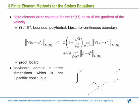
• polyhedral domain in threedimensions which is notLipschitz-continuous
Finite Element Methods for the Simulation of Incompressible Flows · Course at Universidad Autonoma de Madrid, 27.02. – 02.03.2012 · Page 48 (151)
3 Finite Element Methods for the Stokes Equations
• finite element error estimate for the L2(Ω) norm of the gradient of thevelocity Ω⊂ Rd , bounded, polyhedral, Lipschitz-continuous boundary
∥∥∥∇(u−uh)∥∥∥
L2(Ω)≤ 2
(1+
√d
β his
)inf
vh∈V h
∥∥∥∇(u−vh)∥∥∥
L2(Ω)
+√
d infqh∈Qh
∥∥∥p−qh∥∥∥
L2(Ω)
proof: board• polyhedral domain in three
dimensions which is notLipschitz-continuous
Finite Element Methods for the Simulation of Incompressible Flows · Course at Universidad Autonoma de Madrid, 27.02. – 02.03.2012 · Page 48 (151)
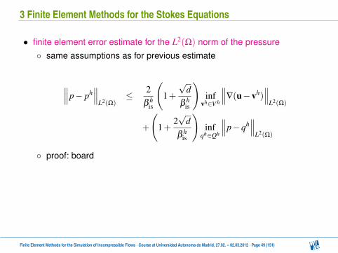
3 Finite Element Methods for the Stokes Equations
• finite element error estimate for the L2(Ω) norm of the pressure same assumptions as for previous estimate
∥∥∥p− ph∥∥∥
L2(Ω)≤ 2
β his
(1+
√d
β his
)inf
vh∈V h
∥∥∥∇(u−vh)∥∥∥
L2(Ω)
+
(1+
2√
dβ h
is
)inf
qh∈Qh
∥∥∥p−qh∥∥∥
L2(Ω)
proof: board
Finite Element Methods for the Simulation of Incompressible Flows · Course at Universidad Autonoma de Madrid, 27.02. – 02.03.2012 · Page 49 (151)

3 Finite Element Methods for the Stokes Equations
• error of the velocity in the L2(Ω) norm by Poincaré inequality not optimal∥∥∥u−uh
∥∥∥L2(Ω)
≤C∥∥∥∇(u−uh)
∥∥∥L2(Ω)
• regular dual Stokes problem: For given f ∈ L2(Ω), find (φ f,ξf) ∈V ×Qsuch that
−∆φ f +∇ξf = f in Ω,
∇ ·φ f = 0 in Ω
regular if mapping (φ f,ξf
)7→ −∆φ f +∇ξf
is an isomorphism from(H2(Ω)∩V
)×(H1(Ω)∩Q
)onto L2(Ω)
Γ of class C2
bounded, convex polygons in two dimensions
Finite Element Methods for the Simulation of Incompressible Flows · Course at Universidad Autonoma de Madrid, 27.02. – 02.03.2012 · Page 50 (151)

3 Finite Element Methods for the Stokes Equations
• finite element error estimate for the L2(Ω) norm of the velocity same assumptions as for previous estimates dual Stokes problem regular with solution (φ f,ξf)∥∥∥u−uh
∥∥∥L2(Ω)
≤√
d(∥∥∥∇
(u−uh
)∥∥∥L2(Ω)
+ infqh∈Qh
∥∥∥p−qh∥∥∥
L2(Ω)
)× sup
f∈L2(Ω)
1∥∥f∥∥
L2(Ω)
[(1+
√d
β his
)inf
φh∈V h
∥∥∥∇
(φ f−φ
h)∥∥∥
L2(Ω)
+ infrh∈Qh
∥∥∥ξf− rh∥∥∥
L2(Ω)
] proof: board (if time admits)
Finite Element Methods for the Simulation of Incompressible Flows · Course at Universidad Autonoma de Madrid, 27.02. – 02.03.2012 · Page 51 (151)
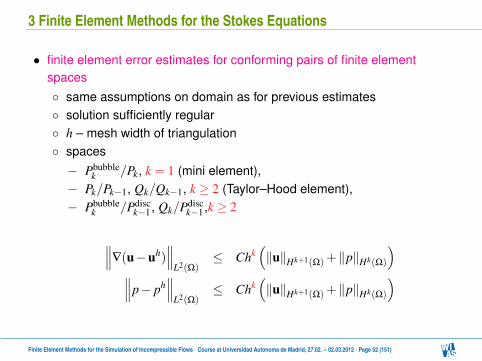
3 Finite Element Methods for the Stokes Equations
• finite element error estimates for conforming pairs of finite elementspaces same assumptions on domain as for previous estimates solution sufficiently regular h – mesh width of triangulation spaces− Pbubble
k /Pk, k = 1 (mini element),− Pk/Pk−1, Qk/Qk−1, k ≥ 2 (Taylor–Hood element),− Pbubble
k /Pdisck−1 , Qk/Pdisc
k−1 ,k ≥ 2
∥∥∥∇(u−uh)∥∥∥
L2(Ω)≤ Chk
(‖u‖Hk+1(Ω)+‖p‖Hk(Ω)
)∥∥∥p− ph
∥∥∥L2(Ω)
≤ Chk(‖u‖Hk+1(Ω)+‖p‖Hk(Ω)
)
Finite Element Methods for the Simulation of Incompressible Flows · Course at Universidad Autonoma de Madrid, 27.02. – 02.03.2012 · Page 52 (151)
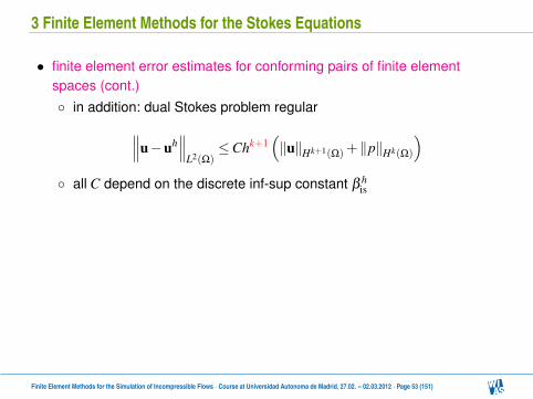
3 Finite Element Methods for the Stokes Equations
• finite element error estimates for conforming pairs of finite elementspaces (cont.) in addition: dual Stokes problem regular∥∥∥u−uh
∥∥∥L2(Ω)
≤Chk+1(‖u‖Hk+1(Ω)+‖p‖Hk(Ω)
) all C depend on the discrete inf-sup constant β h
is
Finite Element Methods for the Simulation of Incompressible Flows · Course at Universidad Autonoma de Madrid, 27.02. – 02.03.2012 · Page 53 (151)
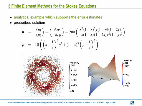
3 Finite Element Methods for the Stokes Equations
• analytical example which supports the error estimates• prescribed solution
u =
(u1
u2
)=
(∂yψ
−∂xψ
)= 200
(x2(1− x)2y(1− y)(1−2y)−x(1− x)(1−2x)y2(1− y)2
)p = 10
((x− 1
2
)3
y2 +(1− x)3(
y− 12
)3)
Finite Element Methods for the Simulation of Incompressible Flows · Course at Universidad Autonoma de Madrid, 27.02. – 02.03.2012 · Page 54 (151)

3 Finite Element Methods for the Stokes Equations
• initial grids (level 0)
• red refinement
Finite Element Methods for the Simulation of Incompressible Flows · Course at Universidad Autonoma de Madrid, 27.02. – 02.03.2012 · Page 55 (151)
3 Finite Element Methods for the Stokes Equations
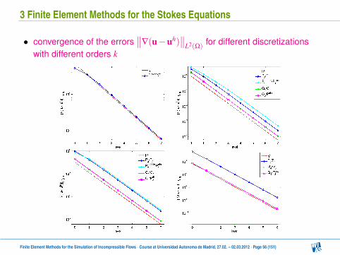
• convergence of the errors∥∥∇(u−uh)
∥∥L2(Ω)
for different discretizationswith different orders k
Finite Element Methods for the Simulation of Incompressible Flows · Course at Universidad Autonoma de Madrid, 27.02. – 02.03.2012 · Page 56 (151)

3 Finite Element Methods for the Stokes Equations
• convergence of the errors∥∥p− ph
∥∥L2(Ω)
for different discretizations withdifferent orders k
Finite Element Methods for the Simulation of Incompressible Flows · Course at Universidad Autonoma de Madrid, 27.02. – 02.03.2012 · Page 57 (151)
3 Finite Element Methods for the Stokes Equations
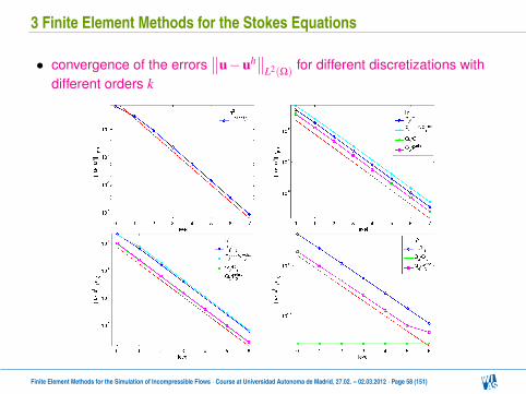
• convergence of the errors∥∥u−uh
∥∥L2(Ω)
for different discretizations withdifferent orders k
Finite Element Methods for the Simulation of Incompressible Flows · Course at Universidad Autonoma de Madrid, 27.02. – 02.03.2012 · Page 58 (151)
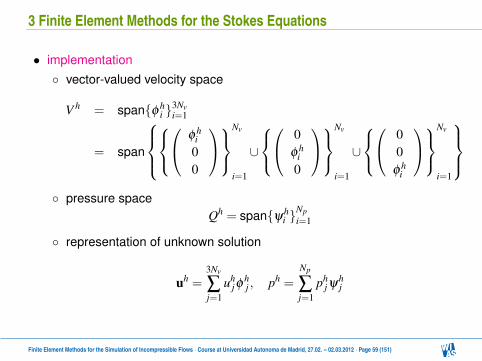
3 Finite Element Methods for the Stokes Equations
• implementation vector-valued velocity space
V h = spanφ hi
3Nvi=1
= span
φ h
i00
Nv
i=1
∪
0
φ hi0
Nv
i=1
∪
0
0φ h
i
Nv
i=1
pressure space
Qh = spanψhi
Npi=1
representation of unknown solution
uh =3Nv
∑j=1
uhjφ
hj , ph =
Np
∑j=1
phjψ
hj
Finite Element Methods for the Simulation of Incompressible Flows · Course at Universidad Autonoma de Madrid, 27.02. – 02.03.2012 · Page 59 (151)
3 Finite Element Methods for the Stokes Equations
• pressure finite element space standard basis functions not in L2
0(Ω)
it can be shown under mild assumptions that standard basis functionscan be used as ansatz and test functions
computed pressure with standard basis functions has to be projectedinto L2
0(Ω) at the end
Finite Element Methods for the Simulation of Incompressible Flows · Course at Universidad Autonoma de Madrid, 27.02. – 02.03.2012 · Page 60 (151)
3 Finite Element Methods for the Stokes Equations
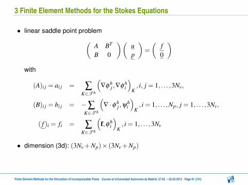
• linear saddle point problem(A BT
B 0
)(up
)=
(f0
)with
(A)i j = ai j = ∑K∈T h
(∇φ
hj ,∇φ
hi
)K, i, j = 1, . . . ,3Nv,
(B)i j = bi j = −∑K∈T h
(∇ ·φ h
j ,ψhi
)K, i = 1, . . . ,Np, j = 1, . . . ,3Nv,
( f )i = fi = ∑K∈T h
(f,φ h
i
)K, i = 1, . . . ,3Nv
• dimension (3d): (3Nv +Np)× (3Nv +Np)
Finite Element Methods for the Simulation of Incompressible Flows · Course at Universidad Autonoma de Madrid, 27.02. – 02.03.2012 · Page 61 (151)

3 Finite Element Methods for the Stokes Equations
• matrix A symmetric positive definite block-diagonal matrix
A =
A11 0 00 A11 00 0 A11
•(D(uh),D(vh))
instead of(∇uh,∇vh
) equivalent only if uh weakly divergence-free generally not given for finite element velocities not longer block-diagonal matrix
A =
A11 A12 A13
AT12 A22 A23
AT13 AT
23 A33
Finite Element Methods for the Simulation of Incompressible Flows · Course at Universidad Autonoma de Madrid, 27.02. – 02.03.2012 · Page 62 (151)

4 The Oseen Equations
• continuous equation
−ν∆u+(b ·∇)u+ cu+∇p = f in Ω,
∇ ·u = 0 in Ω
for simplicity: homogeneous Dirichlet boundary conditions
• difficulties: coupling of velocity and
pressure dominating convection
• properties linear
Carl Wilhelm Oseen (1879 – 1944)
Finite Element Methods for the Simulation of Incompressible Flows · Course at Universidad Autonoma de Madrid, 27.02. – 02.03.2012 · Page 63 (151)

4 The Oseen Equations
• coefficients ν > 0 b ∈W 1,∞(Ω), ∇ ·b = 0 c ∈ L∞(Ω), c(x)≥ c0 ≥ 0
• scaling of momentum equation: one of these possibilities ‖b‖L∞(Ω) = O (1) if ν ≤ ‖b‖L∞(Ω)
ν = O (1) if ‖b‖L∞(Ω) ≤ ν
• interesting cases ν of moderate size, c = 0
in numerical solution of steady-state Navier–Stokes equations ν of arbitrary size, c = O
((∆t)−1
)in numerical solution of time-dependent Navier–Stokes equations
Finite Element Methods for the Simulation of Incompressible Flows · Course at Universidad Autonoma de Madrid, 27.02. – 02.03.2012 · Page 64 (151)

4 The Oseen Equations
• weak form
ν(∇u,∇v)+((b ·∇)u+ cu,v)− (∇ ·v, p) = 〈f,v〉V ′,V ∀ v ∈V,−(∇ ·u,q) = 0 ∀ q ∈ Q
• bilinear forms
a : V ×V → R, a(u,v) = ν(∇u,∇v)+((b ·∇)u+ cu,v),b : V ×Q→ R, b(v,q) = −(∇ ·v,q)
• existence and uniqueness of solution proof: board essential condition
((b ·∇)v,v) = 0 ∀ v ∈V
can be proved is b is weakly divergence-free and has zero trace on Γ
Finite Element Methods for the Simulation of Incompressible Flows · Course at Universidad Autonoma de Madrid, 27.02. – 02.03.2012 · Page 65 (151)

4 The Oseen Equations
• stability of solution dependency of bounds on coefficients is important depending on regularity of data, different estimates possible− most general
ν
2‖∇u‖2
L2(Ω)+∥∥∥c1/2u
∥∥∥2
L2(Ω)≤ 1
2ν‖f‖2
H−1(Ω)
− f ∈ L2(Ω) and c0 > 0
ν ‖∇u‖2L2(Ω)+
12
∥∥∥c1/2u∥∥∥2
L2(Ω)≤ 1
2c0‖f‖2
L2(Ω)
proof: board
estimates for pressure with inf-sup condition discussion: board
Finite Element Methods for the Simulation of Incompressible Flows · Course at Universidad Autonoma de Madrid, 27.02. – 02.03.2012 · Page 66 (151)

4 The Oseen Equations
• stability of solution dependency of bounds on coefficients is important depending on regularity of data, different estimates possible− most general
ν
2‖∇u‖2
L2(Ω)+∥∥∥c1/2u
∥∥∥2
L2(Ω)≤ 1
2ν‖f‖2
H−1(Ω)
− f ∈ L2(Ω) and c0 > 0
ν ‖∇u‖2L2(Ω)+
12
∥∥∥c1/2u∥∥∥2
L2(Ω)≤ 1
2c0‖f‖2
L2(Ω)
proof: board estimates for pressure with inf-sup condition discussion: board
Finite Element Methods for the Simulation of Incompressible Flows · Course at Universidad Autonoma de Madrid, 27.02. – 02.03.2012 · Page 66 (151)
4 The Oseen Equations – Galerkin FEM
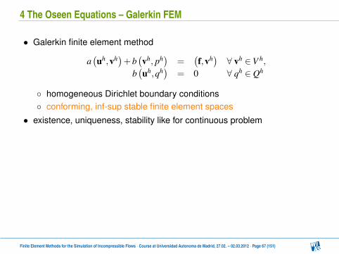
• Galerkin finite element method
a(uh,vh
)+b(vh, ph
)=
(f,vh
)∀ vh ∈V h,
b(uh,qh
)= 0 ∀ qh ∈ Qh
homogeneous Dirichlet boundary conditions conforming, inf-sup stable finite element spaces
• existence, uniqueness, stability like for continuous problem
Finite Element Methods for the Simulation of Incompressible Flows · Course at Universidad Autonoma de Madrid, 27.02. – 02.03.2012 · Page 67 (151)
4 The Oseen Equations – Galerkin FEM
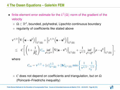
• finite element error estimate for the L2(Ω) norm of the gradient of thevelocity Ω⊂ Rd , bounded, polyhedral, Lipschitz-continuous boundary regularity of coefficients like stated above
ν1/2∥∥∥∇
(u−uh
)∥∥∥L2(Ω)
+∥∥∥c1/2
(u−uh
)∥∥∥L2(Ω)
≤ C
[(1+
1β h
is
)Cos inf
vh∈V h
∥∥∥∇(u−vh)∥∥∥
L2(Ω)+
1ν1/2 inf
qh∈Qh
∥∥∥p−qh∥∥∥
L2(Ω)
],
where
Cos = ν1/2 +‖c‖1/2
L∞(Ω)+‖b‖L∞(Ω) min
1
ν1/2 ,1
c1/20
C does not depend on coefficients and triangulation, but on Ω
(Poincaré–Friedrichs inequality)
Finite Element Methods for the Simulation of Incompressible Flows · Course at Universidad Autonoma de Madrid, 27.02. – 02.03.2012 · Page 68 (151)
4 The Oseen Equations – Galerkin FEM
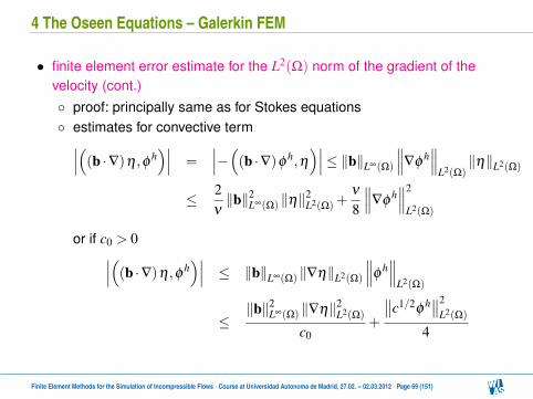
• finite element error estimate for the L2(Ω) norm of the gradient of thevelocity (cont.) proof: principally same as for Stokes equations estimates for convective term∣∣∣((b ·∇)η ,φ h
)∣∣∣ =∣∣∣−((b ·∇)φ
h,η)∣∣∣≤ ‖b‖L∞(Ω)
∥∥∥∇φh∥∥∥
L2(Ω)‖η‖L2(Ω)
≤ 2ν‖b‖2
L∞(Ω) ‖η‖2L2(Ω)+
ν
8
∥∥∥∇φh∥∥∥2
L2(Ω)
or if c0 > 0∣∣∣((b ·∇)η ,φ h)∣∣∣ ≤ ‖b‖L∞(Ω) ‖∇η‖L2(Ω)
∥∥∥φh∥∥∥
L2(Ω)
≤‖b‖2
L∞(Ω) ‖∇η‖2L2(Ω)
c0+
∥∥c1/2φh∥∥2
L2(Ω)
4
Finite Element Methods for the Simulation of Incompressible Flows · Course at Universidad Autonoma de Madrid, 27.02. – 02.03.2012 · Page 69 (151)
4 The Oseen Equations – Galerkin FEM
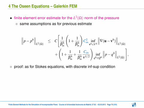
• finite element error estimate for the L2(Ω) norm of the pressure same assumptions as for previous estimate
∥∥∥p− ph∥∥∥
L2(Ω)≤ C
[1
β his
(1+
1β h
is
)C2
os infvh∈V h
∥∥∥∇(u−vh)∥∥∥
L2(Ω)
+
(1+
1β h
is+
1β h
is
Cos
ν1/2
)inf
qh∈Qh
∥∥∥p−qh∥∥∥
L2(Ω)
],
proof: as for Stokes equations, with discrete inf-sup condition
Finite Element Methods for the Simulation of Incompressible Flows · Course at Universidad Autonoma de Madrid, 27.02. – 02.03.2012 · Page 70 (151)
4 The Oseen Equations – Galerkin FEM
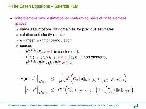
• finite element error estimates for conforming pairs of finite elementspaces same assumptions on domain as for previous estimates solution sufficiently regular h – mesh width of triangulation spaces− Pbubble
k /Pk, k = 1 (mini element),− Pk/Pk−1, Qk/Qk−1, k ≥ 2 (Taylor–Hood element),− Pbubble
k /Pdisck−1 , Qk/Pdisc
k−1 ,k ≥ 2
∥∥∥∇(u−uh)∥∥∥
L2(Ω)≤ C
ν1/2 hk(
Cos ‖u‖Hk+1(Ω)+1
ν1/2 ‖p‖Hk(Ω)
),∥∥∥p− ph
∥∥∥L2(Ω)
≤ Chk(
C2os ‖u‖Hk+1(Ω)+
(1+
Cos
ν1/2
)‖p‖Hk(Ω)
)
Finite Element Methods for the Simulation of Incompressible Flows · Course at Universidad Autonoma de Madrid, 27.02. – 02.03.2012 · Page 71 (151)

4 The Oseen Equations – Galerkin FEM
• Cos for ‖b‖L∞(Ω) = 1
discussion: board• error bounds not uniform for small ν or small time steps
Finite Element Methods for the Simulation of Incompressible Flows · Course at Universidad Autonoma de Madrid, 27.02. – 02.03.2012 · Page 72 (151)
4 The Oseen Equations – Galerkin FEM
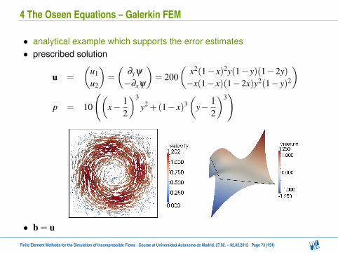
• analytical example which supports the error estimates• prescribed solution
u =
(u1
u2
)=
(∂yψ
−∂xψ
)= 200
(x2(1− x)2y(1− y)(1−2y)−x(1− x)(1−2x)y2(1− y)2
)p = 10
((x− 1
2
)3
y2 +(1− x)3(
y− 12
)3)
• b = u
Finite Element Methods for the Simulation of Incompressible Flows · Course at Universidad Autonoma de Madrid, 27.02. – 02.03.2012 · Page 73 (151)
4 The Oseen Equations – Galerkin FEM
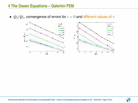
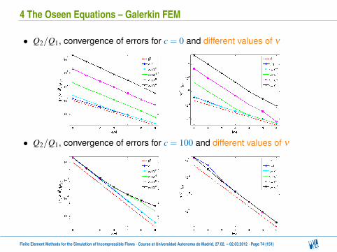
• Q2/Q1, convergence of errors for c = 0 and different values of ν
• Q2/Q1, convergence of errors for c = 100 and different values of ν
Finite Element Methods for the Simulation of Incompressible Flows · Course at Universidad Autonoma de Madrid, 27.02. – 02.03.2012 · Page 74 (151)
4 The Oseen Equations – Galerkin FEM
• Q2/Q1, convergence of errors for c = 0 and different values of ν
• Q2/Q1, convergence of errors for c = 100 and different values of ν
Finite Element Methods for the Simulation of Incompressible Flows · Course at Universidad Autonoma de Madrid, 27.02. – 02.03.2012 · Page 74 (151)

4 The Oseen Equations – Galerkin FEM
• Q2/Q1, convergence of errors for ν = 10−4 and different values of c
• summary Galerkin discretization in some cases unstable
Finite Element Methods for the Simulation of Incompressible Flows · Course at Universidad Autonoma de Madrid, 27.02. – 02.03.2012 · Page 75 (151)

4 The Oseen Equations – Residual-Based Stabilizations
• principal idea• given: linear partial differential equation in strong form
Astrustr = f , f ∈ L2(Ω)
• Galerkin discretization
ah(
uh,vh)=(
f ,vh)∀ vh ∈V h
• needed: modification of strong operator Ahstr : V h→ L2(Ω)
• residualrh(
uh)= Ah
struh− f ∈ L2(Ω)
• generally rh(uh)6= 0
Finite Element Methods for the Simulation of Incompressible Flows · Course at Universidad Autonoma de Madrid, 27.02. – 02.03.2012 · Page 76 (151)
4 The Oseen Equations – Residual-Based Stabilizations
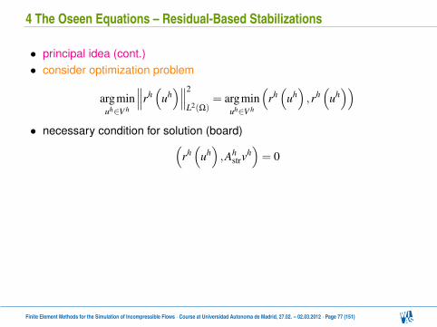
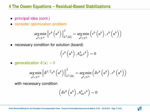
• principal idea (cont.)• consider optimization problem
argminuh∈V h
∥∥∥rh(
uh)∥∥∥2
L2(Ω)= argmin
uh∈V h
(rh(
uh),rh(
uh))
• necessary condition for solution (board)(rh(
uh),Ah
strvh)= 0
• generalization δ (x)> 0
argminuh∈V h
∥∥∥δ1/2rh
(uh)∥∥∥2
L2(Ω)= argmin
uh∈V h
(δ rh(
uh),rh(
uh))
with necessary condition (δ rh(
uh),Ah
strvh)= 0
Finite Element Methods for the Simulation of Incompressible Flows · Course at Universidad Autonoma de Madrid, 27.02. – 02.03.2012 · Page 77 (151)
4 The Oseen Equations – Residual-Based Stabilizations
• principal idea (cont.)• consider optimization problem
argminuh∈V h
∥∥∥rh(
uh)∥∥∥2
L2(Ω)= argmin
uh∈V h
(rh(
uh),rh(
uh))
• necessary condition for solution (board)(rh(
uh),Ah
strvh)= 0
• generalization δ (x)> 0
argminuh∈V h
∥∥∥δ1/2rh
(uh)∥∥∥2
L2(Ω)= argmin
uh∈V h
(δ rh(
uh),rh(
uh))
with necessary condition (δ rh(
uh),Ah
strvh)= 0
Finite Element Methods for the Simulation of Incompressible Flows · Course at Universidad Autonoma de Madrid, 27.02. – 02.03.2012 · Page 77 (151)

4 The Oseen Equations – Residual-Based Stabilizations
• principal idea (cont.)• minimizing residual alone: not good
solid line – function withlayer
dashed line – optimalpiecewise linear approxi-mation
• consider combination
ah(
uh,vh)+(
δ rh(
uh),Ah
strvh)=(
f ,vh)∀ vh ∈V h
optimal choice of weighting function δ (x) by numerical analysis
• example: Oseen equations, board
Finite Element Methods for the Simulation of Incompressible Flows · Course at Universidad Autonoma de Madrid, 27.02. – 02.03.2012 · Page 78 (151)

4 The Oseen Equations – Residual-Based Stabilizations
• principal idea (cont.)• minimizing residual alone: not good
solid line – function withlayer
dashed line – optimalpiecewise linear approxi-mation
• consider combination
ah(
uh,vh)+(
δ rh(
uh),Ah
strvh)=(
f ,vh)∀ vh ∈V h
optimal choice of weighting function δ (x) by numerical analysis• example: Oseen equations, board
Finite Element Methods for the Simulation of Incompressible Flows · Course at Universidad Autonoma de Madrid, 27.02. – 02.03.2012 · Page 78 (151)

4 The Oseen Equations – Residual-Based Stabilizations
• SUPG/PSPG/grad-div stabilization• find
(uh, ph
)∈V h×Qh such that
Aspg
((uh, ph
),(
vh,qh))
= Lspg
((vh,qh
))∀(
vh,qh)∈V h×Qh,
with Aspg :(V × Q
)×(V × Q
)→ R
Aspg ((u, p) ,(v,q))= ν (∇u,∇v)+((b ·∇)u+ cu,v)− (∇ ·v, p)+(∇ ·u,q)
+ ∑K∈T h
µK (∇ ·u,∇ ·v)K + ∑E∈E h
δE ([|p|]E , [|q|]E)E
+ ∑K∈T h
(−ν∆u+(b ·∇)u+ cu+∇p,δ v
K (b ·∇)v+δpK∇q
)K
and Lspg :(V × Q
)→ R
Lspg ((v,q)) = (f,v)+ ∑K∈T h
(f,δ v
K (b ·∇)v+δpK∇q
)K
Finite Element Methods for the Simulation of Incompressible Flows · Course at Universidad Autonoma de Madrid, 27.02. – 02.03.2012 · Page 79 (151)
4 The Oseen Equations – Residual-Based Stabilizations
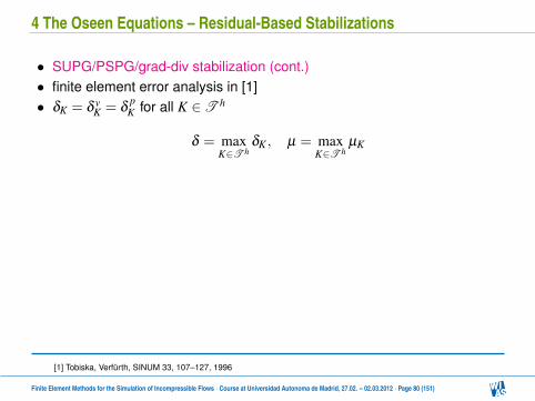
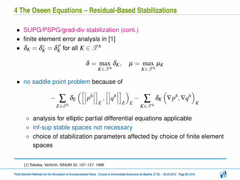
• SUPG/PSPG/grad-div stabilization (cont.)• finite element error analysis in [1]• δK = δ v
K = δpK for all K ∈T h
δ = maxK∈T h
δK , µ = maxK∈T h
µK
• no saddle point problem because of
− ∑E∈E h
δE
([∣∣∣ph∣∣∣]
E,[∣∣∣qh
∣∣∣]E
)E− ∑
K∈T h
δK
(∇ph,∇qh
)K
analysis for elliptic partial differential equations applicable inf-sup stable spaces not necessary choice of stabilization parameters affected by choice of finite element
spaces
[1] Tobiska, Verfürth, SINUM 33, 107–127, 1996
Finite Element Methods for the Simulation of Incompressible Flows · Course at Universidad Autonoma de Madrid, 27.02. – 02.03.2012 · Page 80 (151)
4 The Oseen Equations – Residual-Based Stabilizations
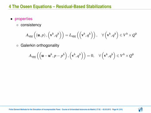
• properties consistency
Aspg
((u, p) ,
(vh,qh
))= Lspg
((vh,qh
)), ∀
(vh,qh
)∈V h×Qh
Galerkin orthogonality
Aspg
((u−uh, p− ph
),(
vh,qh))
= 0, ∀(
vh,qh)∈V h×Qh
Finite Element Methods for the Simulation of Incompressible Flows · Course at Universidad Autonoma de Madrid, 27.02. – 02.03.2012 · Page 81 (151)
4 The Oseen Equations – Residual-Based Stabilizations
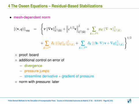
• mesh-dependent norm
‖(v,q)‖spg =
ν ‖∇v‖2
L2(Ω)+∥∥∥c1/2v
∥∥∥2
L2(Ω)+ ∑
K∈T h
µK ‖∇ ·v‖2L2(K)
+ ∑E∈E h
δE ‖[|q|]E‖2L2(E)+ ∑
K∈T h
δK ‖(b ·∇)v+∇q‖2L2(K)
1/2
proof: board additional control on error of− divergence− pressure jumps− streamline derivative + gradient of pressure
norm with pressure: later
Finite Element Methods for the Simulation of Incompressible Flows · Course at Universidad Autonoma de Madrid, 27.02. – 02.03.2012 · Page 82 (151)
4 The Oseen Equations – Residual-Based Stabilizations
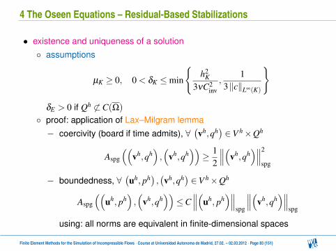
• existence and uniqueness of a solution assumptions
µK ≥ 0, 0 < δK ≤min
h2
K
3νC2inv
,1
3‖c‖L∞(K)
δE > 0 if Qh 6⊂C(Ω)
proof: application of Lax–Milgram lemma− coercivity (board if time admits), ∀
(vh,qh
)∈V h×Qh
Aspg
((vh,qh
),(
vh,qh))≥ 1
2
∥∥∥(vh,qh)∥∥∥2
spg
− boundedness, ∀(uh, ph
),(vh,qh
)∈V h×Qh
Aspg
((uh, ph
),(
vh,qh))≤C
∥∥∥(uh, ph)∥∥∥
spg
∥∥∥(vh,qh)∥∥∥
spg
using: all norms are equivalent in finite-dimensional spaces
Finite Element Methods for the Simulation of Incompressible Flows · Course at Universidad Autonoma de Madrid, 27.02. – 02.03.2012 · Page 83 (151)

4 The Oseen Equations – Residual-Based Stabilizations
• stability
∥∥∥(uh, ph)∥∥∥2
spg≤ 12
5min
‖f‖2
H−1(Ω)
ν,‖f‖2
L2(Ω)
c0
+4 ∑
K∈T h
δK ‖f‖2L2(K)
proof: as usual estimate in stronger norm than for Galerkin finite element method estimate for pressure with inf-sup condition possible
Finite Element Methods for the Simulation of Incompressible Flows · Course at Universidad Autonoma de Madrid, 27.02. – 02.03.2012 · Page 84 (151)

4 The Oseen Equations – Residual-Based Stabilizations
• norm for finite element error estimates
‖(v,q)‖spg,p =(‖(v,q)‖spg +w−2
pres ‖q‖2L2(Ω)
)1/2
withwpres = max
1,ν−1/2,‖c‖1/2
L∞(Ω)
for the interesting cases of small ν and large c: small contribution of thepressure
• first step: inf-sup conditions for Aspg
inf(vh,qh)∈V h×Qh
‖(uh,ph)‖spg,p=1
sup(wh,rh)∈V h×Qh
‖(vh,qh)‖spg,p=1
Aspg
((vh,qh
),(
wh,rh))≥ βspg
some conditions on stabilization parameters, e.g., δ0h2K ≤ δK
proof very technical βspg = O (δ0)
Finite Element Methods for the Simulation of Incompressible Flows · Course at Universidad Autonoma de Madrid, 27.02. – 02.03.2012 · Page 85 (151)
4 The Oseen Equations – Residual-Based Stabilizations
• finite element error estimate∥∥∥(u−uh, p− ph)∥∥∥
spg+ν
1/2∥∥∥p− ph
∥∥∥L2Ω
≤ C
[hk
(ν
1/2 +νδ 1/2
h+
hδ 1/2 +δ
1/2 +µδ 1/2
h+‖c‖1/2
L∞(Ω)h+δ ‖c‖L∞(Ω) h
)‖u‖Hk+1(Ω)
+hl+1
(ν
1/2 +δ 1/2
h+
1ν1/2
(max
1,
µ
ν
)−1/2)‖p‖H l+1(Ω)
]
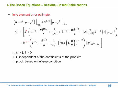
k ≥ 1, l ≥ 0 C independent of the coefficients of the problem proof: based on inf-sup condition
Finite Element Methods for the Simulation of Incompressible Flows · Course at Universidad Autonoma de Madrid, 27.02. – 02.03.2012 · Page 86 (151)

4 The Oseen Equations – Residual-Based Stabilizations
• optimal asymptotics for stabilization parameters, ν < h (board) inf-sup stable discretizations with k = l +1
δ = O(h2) , µ = O (1) =⇒ order of error reduction: k
equal-order discretizations with k = l ≥ 1
O (δ ) = O (µ) = O (h) =⇒ order of error reduction: k+12
• optimal asymptotics for stabilization parameters, ν ≥ h inf-sup stable discretizations with k = l +1
δ = O(h2) , µ = O (1) =⇒ order of convergence: k
equal-order discretizations with k = l ≥ 1
δ = O(h2) , µ arbitrary =⇒ order of convergence: k
Finite Element Methods for the Simulation of Incompressible Flows · Course at Universidad Autonoma de Madrid, 27.02. – 02.03.2012 · Page 87 (151)
4 The Oseen Equations – Residual-Based Stabilizations
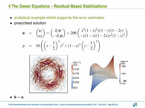
• analytical example which supports the error estimates• prescribed solution
u =
(u1
u2
)=
(∂yψ
−∂xψ
)= 200
(x2(1− x)2y(1− y)(1−2y)−x(1− x)(1−2x)y2(1− y)2
)p = 10
((x− 1
2
)3
y2 +(1− x)3(
y− 12
)3)
• b = u
Finite Element Methods for the Simulation of Incompressible Flows · Course at Universidad Autonoma de Madrid, 27.02. – 02.03.2012 · Page 88 (151)
4 The Oseen Equations – Residual-Based Stabilizations
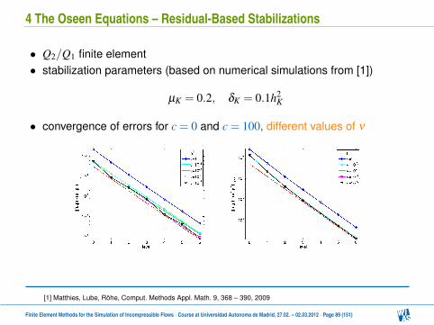
• Q2/Q1 finite element• stabilization parameters (based on numerical simulations from [1])
µK = 0.2, δK = 0.1h2K
• convergence of errors for c = 0 and c = 100, different values of ν
[1] Matthies, Lube, Röhe, Comput. Methods Appl. Math. 9, 368 – 390, 2009
Finite Element Methods for the Simulation of Incompressible Flows · Course at Universidad Autonoma de Madrid, 27.02. – 02.03.2012 · Page 89 (151)
4 The Oseen Equations – Residual-Based Stabilizations
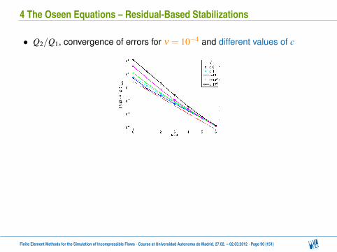
• Q2/Q1, convergence of errors for ν = 10−4 and different values of c
Finite Element Methods for the Simulation of Incompressible Flows · Course at Universidad Autonoma de Madrid, 27.02. – 02.03.2012 · Page 90 (151)
4 The Oseen Equations – Residual-Based Stabilizations
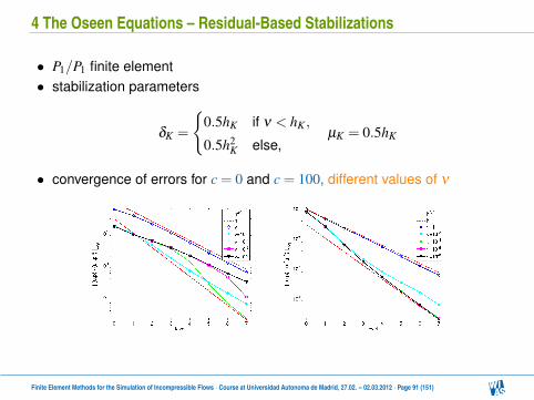
• P1/P1 finite element• stabilization parameters
δK =
0.5hK if ν < hK ,
0.5h2K else,
µK = 0.5hK
• convergence of errors for c = 0 and c = 100, different values of ν
Finite Element Methods for the Simulation of Incompressible Flows · Course at Universidad Autonoma de Madrid, 27.02. – 02.03.2012 · Page 91 (151)
4 The Oseen Equations – Residual-Based Stabilizations
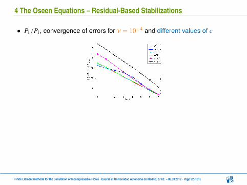
• P1/P1, convergence of errors for ν = 10−4 and different values of c
Finite Element Methods for the Simulation of Incompressible Flows · Course at Universidad Autonoma de Madrid, 27.02. – 02.03.2012 · Page 92 (151)

4 The Oseen Equations – Residual-Based Stabilizations
• implementation: same approach as for Stokes equations• grad-div term leads to matrix blockA11 A12 A13
AT12 A22 A23
AT13 AT
23 A33
instead of
A11 0 00 A11 00 0 A11
• PSPG term introduces pressure-pressure couplings• SUPG term influences velocity-velocity coupling and the pressure
(ansatz) - velocity (test) coupling• final system (
A DB C
)(up
)=
(ffp
)much more matrix blocks to store than for Galerkin FEM
Finite Element Methods for the Simulation of Incompressible Flows · Course at Universidad Autonoma de Madrid, 27.02. – 02.03.2012 · Page 93 (151)

4 The Oseen Equations – Residual-Based Stabilizations
• Summary and remarks errors
∥∥(u, p)− (uh, ph)∥∥
spg independent of ν
versions without pressure couplings available− only for inf-sup stable pairs of finite elements− easier to implement than SUPG/PSPG/grad-div stabilization
numerical analysis in [1,2,3]
[1] Tobiska, Verfürth, SINUM 33, 107–127, 1996
[2] Lube, Rapin, M3AS 16, 949–966, 2006
[3] Matthies, Lube, Röhe, Comput. Methods Appl. Math. 9, 368–390, 2009
Finite Element Methods for the Simulation of Incompressible Flows · Course at Universidad Autonoma de Madrid, 27.02. – 02.03.2012 · Page 94 (151)
5 The Stationary Navier–Stokes Equations
• continuous equation
−ν∆u+(u ·∇)u+∇p = f in Ω,
∇ ·u = 0 in Ω
for simplicity: homogeneous Dirichlet boundary conditions• difficulties: coupling of velocity and pressure dominating convection nonlinear
Finite Element Methods for the Simulation of Incompressible Flows · Course at Universidad Autonoma de Madrid, 27.02. – 02.03.2012 · Page 95 (151)
5 The Stationary Navier–Stokes Equations
• different forms of the convective term
(u ·∇)u : convective form,
∇ ·(uuT ) : divergence form,
(∇×u)×u : rotational form
convective form and divergence form equivalent if ∇ ·u = 0 (board, iftime permits)
convective form and rotational form
(∇×u)×u+12
∇(uT u
)= (u ·∇)u
definition of new pressure (Bernoulli pressure) in rotational form
pBern = p+12
uT u
Finite Element Methods for the Simulation of Incompressible Flows · Course at Universidad Autonoma de Madrid, 27.02. – 02.03.2012 · Page 96 (151)
5 The Stationary Navier–Stokes Equations
• variational form of the steady-state Navier–Stokes equations: Find(u, p) ∈V ×Q such that
(ν∇u,∇v)+((u ·∇)u,v)− (∇ ·v, p) = (f,v)−(∇ ·u,q) = 0
for all (v,q) ∈V ×Q• equivalent: Find (u, p) ∈V ×Q such that
(ν∇u,∇v)+((u ·∇)u,v)− (∇ ·v, p)+(∇ ·u,q) = (f,v)
for all (v,q) ∈V ×Q
Finite Element Methods for the Simulation of Incompressible Flows · Course at Universidad Autonoma de Madrid, 27.02. – 02.03.2012 · Page 97 (151)
5 The Stationary Navier–Stokes Equations
• properties of convective term linear in each component (trilinear) u,v,w ∈ H1(Ω), product rule
((u ·∇)v,w) =(∇ ·(vuT ) ,w)− ((∇ ·u)v,w)
u,v,w ∈ H1(Ω), product rule
((u ·∇)v,w) = (u,∇(v ·w))− ((u ·∇)w,v)
Finite Element Methods for the Simulation of Incompressible Flows · Course at Universidad Autonoma de Madrid, 27.02. – 02.03.2012 · Page 98 (151)
5 The Stationary Navier–Stokes Equations
• convective terms in the variational formulation convective form
nconv(u,v,w) = ((u ·∇)v,w)
divergence form
ndiv(u,v,w) = nconv(u,v,w)+((∇ ·u)v,w)
rotational formnrot(u,v,w) = ((∇×u)×v,w)
with momentum equation
(ν∇u,∇v)+nrot(u,u,v)− (∇ ·v, pBern) = (f,v) ∀ v ∈V,
skew-symmetric form (for u weakly divergence-free, u ·n = 0 on Γ,board)
nskew(u,v,w) =12(nconv(u,v,w)−nconv(u,w,v))
Finite Element Methods for the Simulation of Incompressible Flows · Course at Universidad Autonoma de Madrid, 27.02. – 02.03.2012 · Page 99 (151)
5 The Stationary Navier–Stokes Equations
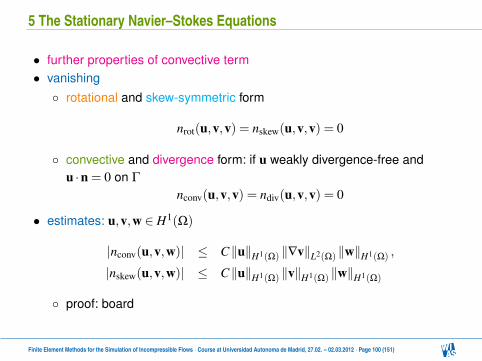
• further properties of convective term• vanishing rotational and skew-symmetric form
nrot(u,v,v) = nskew(u,v,v) = 0
convective and divergence form: if u weakly divergence-free andu ·n = 0 on Γ
nconv(u,v,v) = ndiv(u,v,v) = 0
• estimates: u,v,w ∈ H1(Ω)
|nconv(u,v,w)| ≤ C‖u‖H1(Ω) ‖∇v‖L2(Ω) ‖w‖H1(Ω) ,
|nskew(u,v,w)| ≤ C‖u‖H1(Ω) ‖v‖H1(Ω) ‖w‖H1(Ω)
proof: board
Finite Element Methods for the Simulation of Incompressible Flows · Course at Universidad Autonoma de Madrid, 27.02. – 02.03.2012 · Page 100 (151)
5 The Stationary Navier–Stokes Equations
• further properties of convective term• vanishing rotational and skew-symmetric form
nrot(u,v,v) = nskew(u,v,v) = 0
convective and divergence form: if u weakly divergence-free andu ·n = 0 on Γ
nconv(u,v,v) = ndiv(u,v,v) = 0
• estimates: u,v,w ∈ H1(Ω)
|nconv(u,v,w)| ≤ C‖u‖H1(Ω) ‖∇v‖L2(Ω) ‖w‖H1(Ω) ,
|nskew(u,v,w)| ≤ C‖u‖H1(Ω) ‖v‖H1(Ω) ‖w‖H1(Ω)
proof: board
Finite Element Methods for the Simulation of Incompressible Flows · Course at Universidad Autonoma de Madrid, 27.02. – 02.03.2012 · Page 100 (151)
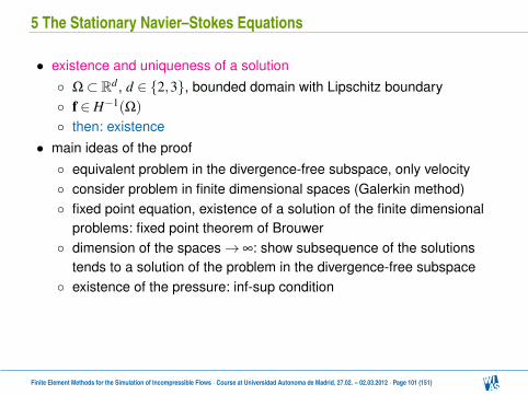
5 The Stationary Navier–Stokes Equations
• existence and uniqueness of a solution Ω⊂ Rd , d ∈ 2,3, bounded domain with Lipschitz boundary f ∈ H−1(Ω)
then: existence• main ideas of the proof equivalent problem in the divergence-free subspace, only velocity consider problem in finite dimensional spaces (Galerkin method) fixed point equation, existence of a solution of the finite dimensional
problems: fixed point theorem of Brouwer dimension of the spaces→ ∞: show subsequence of the solutions
tends to a solution of the problem in the divergence-free subspace existence of the pressure: inf-sup condition
Finite Element Methods for the Simulation of Incompressible Flows · Course at Universidad Autonoma de Madrid, 27.02. – 02.03.2012 · Page 101 (151)
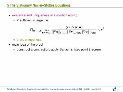
5 The Stationary Navier–Stokes Equations
• existence and uniqueness of a solution (cont.) ν sufficiently large, i.e.
‖f‖H−1(Ω) supu,v,w∈V
((u ·∇)v,w)
‖∇u‖L2(Ω) ‖∇v‖L2(Ω) ‖∇w‖L2(Ω)
< ν2
then: uniqueness• main idea of the proof construct a contraction, apply Banach’s fixed point theorem
• numerical simulations case of unique solution is of interest steady-state solutions unstable in non-unique case, solve
time-dependent solution
Finite Element Methods for the Simulation of Incompressible Flows · Course at Universidad Autonoma de Madrid, 27.02. – 02.03.2012 · Page 102 (151)

5 The Stationary Navier–Stokes Equations
• stability
‖∇u‖L2(Ω) ≤1ν‖f‖H−1(Ω) ,
‖p‖L2(Ω) ≤1
βis
(2‖f‖H−1(Ω)+
Cν2 ‖f‖
2H−1(Ω)
) proof: as usual, using
n(u,u,u) = 0
Finite Element Methods for the Simulation of Incompressible Flows · Course at Universidad Autonoma de Madrid, 27.02. – 02.03.2012 · Page 103 (151)

5 The Stationary Navier–Stokes Equations – Galerkin FEM
• Galerkin finite element method
ν(∇uh,∇vh
)+n(uh,uh,vh
)−(∇ ·vh, ph
)=
(f,vh
)∀ vh ∈V h,
−(∇ ·uh,qh
)= 0 ∀ qh ∈ Qh,
• inf-sup stable pair of finite element spaces
• finite element error analysis for nskew(·, ·, ·)
nskew
(uh,vh,vh
)=
12
(nconv
(uh,vh,vh
)−nconv
(uh,vh,vh
))= 0
note that in general uh 6∈Vdiv =⇒
nconv
(uh,vh,vh
)6= 0, ndiv
(uh,vh,vh
)6= 0
• same as for continuous problem: existence, uniqueness stability
Finite Element Methods for the Simulation of Incompressible Flows · Course at Universidad Autonoma de Madrid, 27.02. – 02.03.2012 · Page 104 (151)
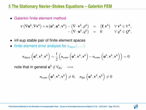
5 The Stationary Navier–Stokes Equations – Galerkin FEM
• Galerkin finite element method
ν(∇uh,∇vh
)+n(uh,uh,vh
)−(∇ ·vh, ph
)=
(f,vh
)∀ vh ∈V h,
−(∇ ·uh,qh
)= 0 ∀ qh ∈ Qh,
• inf-sup stable pair of finite element spaces• finite element error analysis for nskew(·, ·, ·)
nskew
(uh,vh,vh
)=
12
(nconv
(uh,vh,vh
)−nconv
(uh,vh,vh
))= 0
note that in general uh 6∈Vdiv =⇒
nconv
(uh,vh,vh
)6= 0, ndiv
(uh,vh,vh
)6= 0
• same as for continuous problem: existence, uniqueness stability
Finite Element Methods for the Simulation of Incompressible Flows · Course at Universidad Autonoma de Madrid, 27.02. – 02.03.2012 · Page 104 (151)

5 The Stationary Navier–Stokes Equations – Galerkin FEM
• Finite element error estimate for the L2(Ω) norm of the gradient of thevelocity Ω⊂ Rd bounded domain with polyhedral boundary ν−2 ‖f‖H−1(Ω) be sufficiently small such that unique solution
inf-sup stable finite element spaces V h×Qh∥∥∥∇(u−uh)∥∥∥
L2(Ω)
≤ C
((1+
1ν2 ‖f‖H−1(Ω)
)(1+
1β h
is
)inf
vh∈V h
∥∥∥∇
(u−vh
)∥∥∥L2(Ω)
+1ν
infqh∈Qh
∥∥∥p−qh∥∥∥
L2(Ω)
) proof: main ideas and treatment of nonlinear term: board
Finite Element Methods for the Simulation of Incompressible Flows · Course at Universidad Autonoma de Madrid, 27.02. – 02.03.2012 · Page 105 (151)

5 The Stationary Navier–Stokes Equations – Galerkin FEM
• Finite element error estimate for the L2(Ω) norm of the pressure∥∥∥p− ph∥∥∥
L2(Ω)
≤ Cν
β his
((1+
1ν2 ‖f‖H−1(Ω)
)2(
1+1
β his
)inf
vh∈V h
∥∥∥∇
(u−vh
)∥∥∥L2(Ω)
+Cν
β his
(1+
1ν2 ‖f‖H−1(Ω)
)inf
qh∈Qh
∥∥∥p−qh∥∥∥
L2(Ω)
)
• analytical results can be supported numerically by analytical testexamples
Finite Element Methods for the Simulation of Incompressible Flows · Course at Universidad Autonoma de Madrid, 27.02. – 02.03.2012 · Page 106 (151)
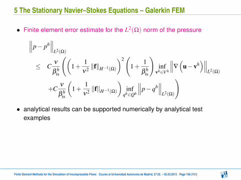

5 The Stationary Navier–Stokes Equations – Galerkin FEM
• Example: steady-state flow around a cylinder at Re = 20 domain
velocity
pressure
Finite Element Methods for the Simulation of Incompressible Flows · Course at Universidad Autonoma de Madrid, 27.02. – 02.03.2012 · Page 107 (151)

5 The Stationary Navier–Stokes Equations – Galerkin FEM
• Example: steady-state flow around a cylinder at Re = 20 at the cylinder
Finite Element Methods for the Simulation of Incompressible Flows · Course at Universidad Autonoma de Madrid, 27.02. – 02.03.2012 · Page 108 (151)
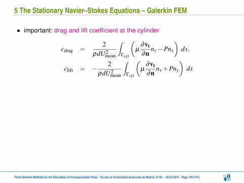
5 The Stationary Navier–Stokes Equations – Galerkin FEM
• important: drag and lift coefficient at the cylinder
cdrag =2
ρdU2mean
∫Γcyl
(µ
∂vt
∂nny−Pnx
)ds,
clift = − 2ρdU2
mean
∫Γcyl
(µ
∂vt
∂nnx +Pny
)ds
• reformulation with volume integrals possible, long but elementaryderivation, e.g.
cdrag =−2U2
dU2mean
((ν∇u,∇wd)+n(u,u,wd)− (∇ ·wd , p)− (f,wd)
)for any function wd ∈ H1(Ω) with wd = 0 on Γ\Γcyl and wd |Γcyl = (1,0)T
Finite Element Methods for the Simulation of Incompressible Flows · Course at Universidad Autonoma de Madrid, 27.02. – 02.03.2012 · Page 109 (151)
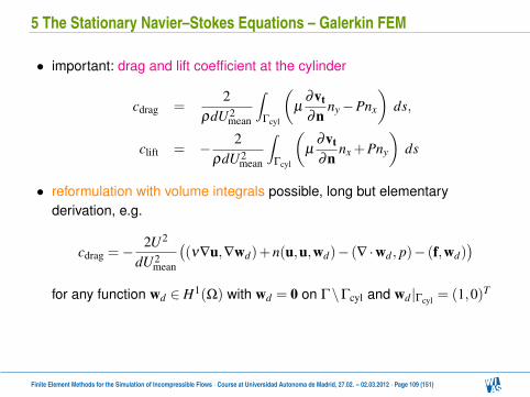

5 The Stationary Navier–Stokes Equations – Galerkin FEM
• reference values [1] : compiled from simulations of different groups
cdrag,ref ∈ [5.57,5.59], clift,ref ∈ [0.104,0.110]
[2] : do-nothing conditions at outlet
cdrag,ref = 5.57953523384, clift,ref = 0.010618948146
[3] : Dirichlet conditions at outlet
cdrag,ref = 5.57953523384, clift,ref = 0.010618937712
[1] Schäfer, Turek, Notes on Numerical Fluid Mechanics 52, 547–566, 1996
[2] Nabh, PhD thesis, Heidelberg, 1998
[3] J., Matthies, IJNMF 37, 885–903, 2001
Finite Element Methods for the Simulation of Incompressible Flows · Course at Universidad Autonoma de Madrid, 27.02. – 02.03.2012 · Page 110 (151)
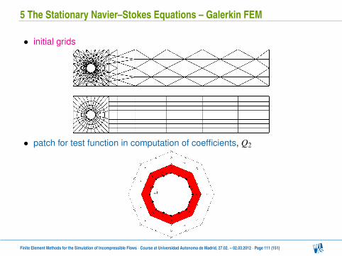
5 The Stationary Navier–Stokes Equations – Galerkin FEM
• initial grids
• patch for test function in computation of coefficients, Q2
Finite Element Methods for the Simulation of Incompressible Flows · Course at Universidad Autonoma de Madrid, 27.02. – 02.03.2012 · Page 111 (151)

5 The Stationary Navier–Stokes Equations – Galerkin FEM
• convective form of convective term• do-nothing boundary conditions• convergence of drag coefficient
Finite Element Methods for the Simulation of Incompressible Flows · Course at Universidad Autonoma de Madrid, 27.02. – 02.03.2012 · Page 112 (151)

5 The Stationary Navier–Stokes Equations – Galerkin FEM
• convergence of lift coefficient
Finite Element Methods for the Simulation of Incompressible Flows · Course at Universidad Autonoma de Madrid, 27.02. – 02.03.2012 · Page 113 (151)

5 The Stationary Navier–Stokes Equations – Galerkin FEM
• preliminary results: different forms of the convective term, P2/P1
• rotational form reconstructed pressure has boundary layers, inaccurate results
Finite Element Methods for the Simulation of Incompressible Flows · Course at Universidad Autonoma de Madrid, 27.02. – 02.03.2012 · Page 114 (151)

5 The Stationary Navier–Stokes Equations – Galerkin FEM
• schemes for solving the nonlinearity• fixed point iteration(
u(m+1)
p(m+1)
)=
(u(m)
p(m)
)−ϑN−1
lin
(((f,v)−N
(u(m);u(m), p(m)
)0
))
with
N(w;u, p) =(
a(u,v)+n(w,u,v)+b(v, p)b(u,q)
)Nlin – linear operatorϑ ∈ (0,1] – damping factor
Finite Element Methods for the Simulation of Incompressible Flows · Course at Universidad Autonoma de Madrid, 27.02. – 02.03.2012 · Page 115 (151)
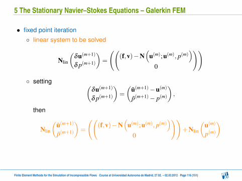
5 The Stationary Navier–Stokes Equations – Galerkin FEM
• fixed point iteration linear system to be solved
Nlin
(δu(m+1)
δ p(m+1)
)=
(((f,v)−N
(u(m);u(m), p(m)
)0
))
setting (δu(m+1)
δ p(m+1)
)=
(u(m+1)−u(m)
p(m+1)− p(m)
),
then
Nlin
(u(m+1)
p(m+1)
)=
(((f,v)−N
(u(m);u(m), p(m)
)0
))+Nlin
(u(m)
p(m)
)
Finite Element Methods for the Simulation of Incompressible Flows · Course at Universidad Autonoma de Madrid, 27.02. – 02.03.2012 · Page 116 (151)
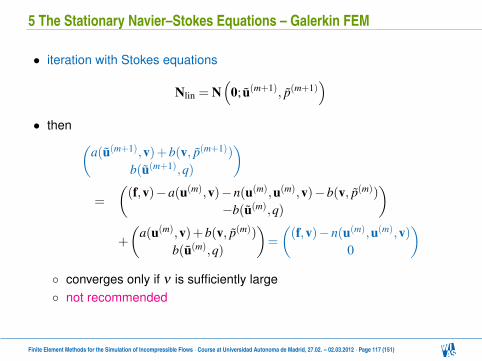
5 The Stationary Navier–Stokes Equations – Galerkin FEM
• iteration with Stokes equations
Nlin = N(
0; u(m+1), p(m+1))
• then (a(u(m+1),v)+b(v, p(m+1))
b(u(m+1),q)
)=
((f,v)−a(u(m),v)−n(u(m),u(m),v)−b(v, p(m))
−b(u(m),q)
)+
(a(u(m),v)+b(v, p(m))
b(u(m),q)
)=
((f,v)−n(u(m),u(m),v)
0
) converges only if ν is sufficiently large not recommended
Finite Element Methods for the Simulation of Incompressible Flows · Course at Universidad Autonoma de Madrid, 27.02. – 02.03.2012 · Page 117 (151)
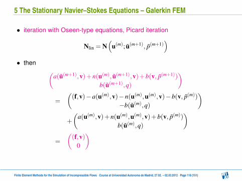
5 The Stationary Navier–Stokes Equations – Galerkin FEM
• iteration with Oseen-type equations, Picard iteration
Nlin = N(
u(m); u(m+1), p(m+1))
• then (a(u(m+1),v)+n(u(m), u(m+1),v)+b(v, p(m+1))
b(u(m+1),q)
)=
((f,v)−a(u(m),v)−n(u(m),u(m),v)−b(v, p(m))
−b(u(m),q)
)+
(a(u(m),v)+n(u(m),u(m),v)+b(v, p(m))
b(u(m),q)
)=
((f,v)
0
)
Finite Element Methods for the Simulation of Incompressible Flows · Course at Universidad Autonoma de Madrid, 27.02. – 02.03.2012 · Page 118 (151)
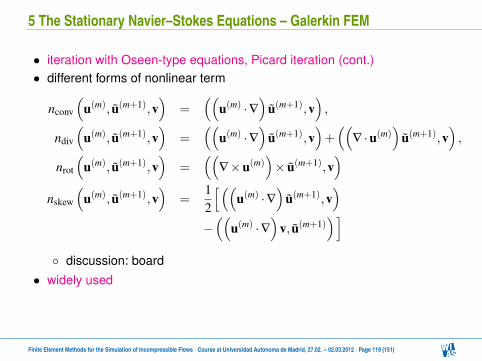
5 The Stationary Navier–Stokes Equations – Galerkin FEM
• iteration with Oseen-type equations, Picard iteration (cont.)• different forms of nonlinear term
nconv
(u(m), u(m+1),v
)=
((u(m) ·∇
)u(m+1),v
),
ndiv
(u(m), u(m+1),v
)=
((u(m) ·∇
)u(m+1),v
)+((
∇ ·u(m))
u(m+1),v),
nrot
(u(m), u(m+1),v
)=
((∇×u(m)
)× u(m+1),v
)nskew
(u(m), u(m+1),v
)=
12
[((u(m) ·∇
)u(m+1),v
)−((
u(m) ·∇)
v, u(m+1))]
discussion: board• widely used
Finite Element Methods for the Simulation of Incompressible Flows · Course at Universidad Autonoma de Madrid, 27.02. – 02.03.2012 · Page 119 (151)

5 The Stationary Navier–Stokes Equations – Galerkin FEM
• Newton’s method• linear operator is derivative of the nonlinear operator at the current
position
Nlin = DN(
u(m)
p(m)
) with Gâteaux derivative at (u, p)T
DN(
up
)= lim
ε→0
N(u+ εφ ;u+ εφ , p+ εψ)−N(u;u, p)ε
= N(φ ;u, p)+N(u;φ , p)+N(u,u,ψ)
inserting and collecting terms (board)(a(u(m+1),v)+n(u(m), u(m+1),v)+n(u(m+1),u(m),v)+b(v, p(m+1))
b(u(m+1),q)
)=
((f,v)+n(u(m),u(m),v)
0
)Finite Element Methods for the Simulation of Incompressible Flows · Course at Universidad Autonoma de Madrid, 27.02. – 02.03.2012 · Page 120 (151)
5 The Stationary Navier–Stokes Equations – Galerkin FEM
• Newton’s method (cont.) order of convergence of Newton’s method expected to be better than
of the Picard iteration if− the solution (u, p) is sufficiently smooth− the linear systems are solved sufficiently accurately
properties of term n(u(m+1),u(m),v) not clear sometimes used in practice
Finite Element Methods for the Simulation of Incompressible Flows · Course at Universidad Autonoma de Madrid, 27.02. – 02.03.2012 · Page 121 (151)

5 The Stationary Navier–Stokes Equations – Galerkin FEM
• implementation same principal approach as for Stokes and Oseen equations inf-sup stable finite elements lead to linear saddle point problems in
fixed point iteration (A BT
B 0
)(up
)=
(f0
)
convective form of convective term− Picard iteration
A =
A11 0 00 A11 00 0 A11
− Newton iteration
A =
A11 A12 A13
A21 A22 A23
A31 A32 A33
Finite Element Methods for the Simulation of Incompressible Flows · Course at Universidad Autonoma de Madrid, 27.02. – 02.03.2012 · Page 122 (151)
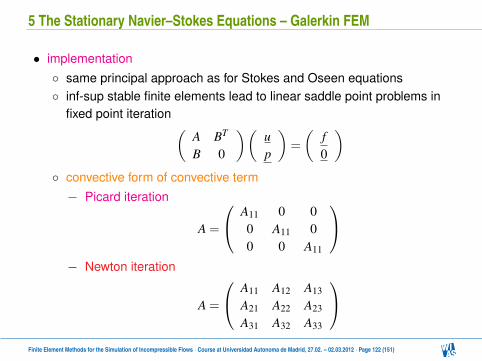
5 The Stationary Navier–Stokes Equations – Galerkin FEM
• implementation same principal approach as for Stokes and Oseen equations inf-sup stable finite elements lead to linear saddle point problems in
fixed point iteration (A BT
B 0
)(up
)=
(f0
) convective form of convective term− Picard iteration
A =
A11 0 00 A11 00 0 A11
− Newton iteration
A =
A11 A12 A13
A21 A22 A23
A31 A32 A33
Finite Element Methods for the Simulation of Incompressible Flows · Course at Universidad Autonoma de Madrid, 27.02. – 02.03.2012 · Page 122 (151)
5 The Stationary Navier–Stokes Equations – Galerkin FEM
• residual-based (and other) stabilizations possible better: solve time-dependent problem
Finite Element Methods for the Simulation of Incompressible Flows · Course at Universidad Autonoma de Madrid, 27.02. – 02.03.2012 · Page 123 (151)
6 The Time-Dependent NSE – Laminar Flows
• continuous equation
∂tu−ν∆u+(u ·∇)u+∇p = f in (0,T ]×Ω,
∇ ·u = 0 in [0,T ]×Ω,
u(0, ·) = u0 in Ω,
withu = 0 in [0,T ]×Γ
Finite Element Methods for the Simulation of Incompressible Flows · Course at Universidad Autonoma de Madrid, 27.02. – 02.03.2012 · Page 124 (151)
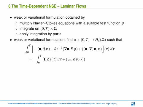
6 The Time-Dependent NSE – Laminar Flows
• weak or variational formulation obtained by multiply Navier–Stokes equations with a suitable test function ϕ
integrate on (0,T )×Ω
apply integration by parts• weak or variational formulation: find u : (0,T ]→ H1
0 (Ω) such that∫ T
0
[− (u,∂tϕ)+Re−1 (∇u,∇ϕ)+((u ·∇)u,ϕ)
](τ) dτ
=∫ T
0(f,ϕ)(τ) dτ +(u0,ϕ (0, ·))
• properties no time derivative with respect to u no second order space derivative with respect to u the pressure vanished because∫
Ω
∇p ·ϕ dx = (∇p,ϕ) =∫
Γ
p(s)ϕ(s)︸︷︷︸=0
·n(s) ds− (p,∇ ·ϕ︸︷︷︸=0
) = 0
Finite Element Methods for the Simulation of Incompressible Flows · Course at Universidad Autonoma de Madrid, 27.02. – 02.03.2012 · Page 125 (151)

6 The Time-Dependent NSE – Laminar Flows
• mathematical analysis 2d: existence and uniqueness of weak solution, Leary (1933), Hopf
(1951) 3d: existence of weak solution, Leary (1933), Hopf (1951)
• Jean Leray (1906 – 1998) Eberhard Hopf (1902 – 1983)
Uniqueness of weak solution of 3d Navier–Stokes equations is openproblem !
Finite Element Methods for the Simulation of Incompressible Flows · Course at Universidad Autonoma de Madrid, 27.02. – 02.03.2012 · Page 126 (151)
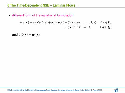
6 The Time-Dependent NSE – Laminar Flows
• different form of the variational formulation
(∂tu,v)+ν (∇u,∇v)+n(u,u,v)− (∇ ·v, p) = (f,v) ∀ v ∈V,−(∇ ·u,q) = 0 ∀ q ∈ Q,
and u(0,x) = u0(x)
• stability of velocity (board)
‖u(T )‖2L2(Ω)+ν ‖∇u‖2
L2(0,T ;L2(Ω)) ≤ ‖u(0)‖2L2(Ω)+
1ν‖f‖2
L2(0,T ;H−1(Ω))
Finite Element Methods for the Simulation of Incompressible Flows · Course at Universidad Autonoma de Madrid, 27.02. – 02.03.2012 · Page 127 (151)

6 The Time-Dependent NSE – Laminar Flows
• different form of the variational formulation
(∂tu,v)+ν (∇u,∇v)+n(u,u,v)− (∇ ·v, p) = (f,v) ∀ v ∈V,−(∇ ·u,q) = 0 ∀ q ∈ Q,
and u(0,x) = u0(x)• stability of velocity (board)
‖u(T )‖2L2(Ω)+ν ‖∇u‖2
L2(0,T ;L2(Ω)) ≤ ‖u(0)‖2L2(Ω)+
1ν‖f‖2
L2(0,T ;H−1(Ω))
Finite Element Methods for the Simulation of Incompressible Flows · Course at Universidad Autonoma de Madrid, 27.02. – 02.03.2012 · Page 127 (151)
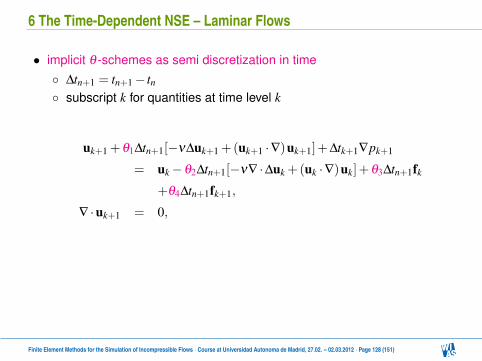
6 The Time-Dependent NSE – Laminar Flows
• implicit θ -schemes as semi discretization in time ∆tn+1 = tn+1− tn subscript k for quantities at time level k
uk+1 +θ1∆tn+1[−ν∆uk+1 +(uk+1 ·∇)uk+1]+∆tk+1∇pk+1
= uk−θ2∆tn+1[−ν∇ ·∆uk +(uk ·∇)uk]+θ3∆tn+1fk
+θ4∆tn+1fk+1,
∇ ·uk+1 = 0,
• one-step θ -schemes: n = kθ1 θ2 θ3 θ4 tk tk+1 ∆tk+1 order
forward Euler scheme 0 1 1 0 tn tn+1 ∆tn+1backward Euler scheme (BWE) 1 0 0 1 tn tn+1 ∆tn+1 1Crank–Nicolson scheme (CN) 0.5 0.5 0.5 0.5 tn tn+1 ∆tn+1 2
Finite Element Methods for the Simulation of Incompressible Flows · Course at Universidad Autonoma de Madrid, 27.02. – 02.03.2012 · Page 128 (151)
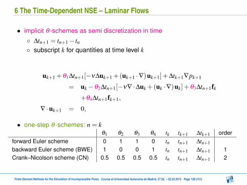
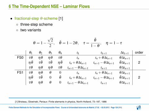
6 The Time-Dependent NSE – Laminar Flows
• fractional-step θ -scheme [1] three-step scheme two variants
θ = 1−√
22
, θ = 1−2θ , τ =θ
1−θ, η = 1− τ
θ1 θ2 θ3 θ4 tk tk+1 ∆tk+1 orderFS0 τθ ηθ ηθ τθ tn tn +θ∆tn+1 θ∆tn+1
ηθ τθ τθ ηθ tn +θ∆tn+1 tn+1−θ∆tn+1 θ∆tn+1 2τθ ηθ ηθ τθ tn+1−θ∆tn+1 tn+1 θ∆tn+1
FS1 τθ ηθ θ 0 tn tn +θ∆tn+1 θ∆tn+1ηθ τθ 0 θ tn +θ∆tn+1 tn+1−θ∆tn+1 θ∆tn+1 2τθ ηθ θ 0 tn+1−θ∆tn+1 tn+1 θ∆tn+1
[1] Bristeau, Glowinski, Periaux: Finite elements in physics, North-Holland, 73–187, 1986
Finite Element Methods for the Simulation of Incompressible Flows · Course at Universidad Autonoma de Madrid, 27.02. – 02.03.2012 · Page 129 (151)

6 The Time-Dependent NSE – Laminar Flows
• popular approaches: BWE, CN• stability BWE, FS0, FS1: strongly A-stable CN: A-stable
• FS1 less expensive than FS0 if computation of right hand side costly
• number of papers with finite element error estimates available proofs become long same techniques as for steady-state problems + Gronwall’s lemma
Finite Element Methods for the Simulation of Incompressible Flows · Course at Universidad Autonoma de Madrid, 27.02. – 02.03.2012 · Page 130 (151)

6 The Time-Dependent NSE – Laminar Flows
• popular approaches: BWE, CN• stability BWE, FS0, FS1: strongly A-stable CN: A-stable
• FS1 less expensive than FS0 if computation of right hand side costly• number of papers with finite element error estimates available proofs become long same techniques as for steady-state problems + Gronwall’s lemma
Finite Element Methods for the Simulation of Incompressible Flows · Course at Universidad Autonoma de Madrid, 27.02. – 02.03.2012 · Page 130 (151)
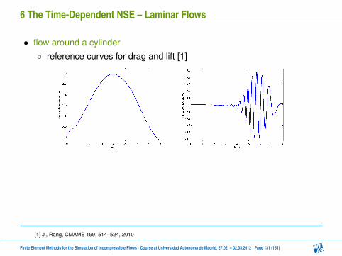
6 The Time-Dependent NSE – Laminar Flows
• flow around a cylinder reference curves for drag and lift [1]
[1] J., Rang, CMAME 199, 514–524, 2010
Finite Element Methods for the Simulation of Incompressible Flows · Course at Universidad Autonoma de Madrid, 27.02. – 02.03.2012 · Page 131 (151)

6 The Time-Dependent NSE – Laminar Flows
• refinement in space with Q2/Pdisc1
P2/P1 Q2/Pdisc1
level velocity pressure all velocity pressure all3 25 408 3248 28 656 27 232 9984 37 2164 100 480 12 704 113 184 107 712 39 936 147 6485 399 616 50 240 449 856 428 416 159 744 588 160
• refinement in time: ∆t ∈ 0.02,0.01,0.005
Finite Element Methods for the Simulation of Incompressible Flows · Course at Universidad Autonoma de Madrid, 27.02. – 02.03.2012 · Page 132 (151)
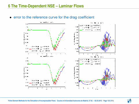
6 The Time-Dependent NSE – Laminar Flows
• error to the reference curve for the drag coefficient
Finite Element Methods for the Simulation of Incompressible Flows · Course at Universidad Autonoma de Madrid, 27.02. – 02.03.2012 · Page 133 (151)
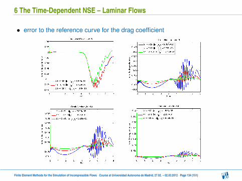
6 The Time-Dependent NSE – Laminar Flows
• error to the reference curve for the drag coefficient
Finite Element Methods for the Simulation of Incompressible Flows · Course at Universidad Autonoma de Madrid, 27.02. – 02.03.2012 · Page 134 (151)
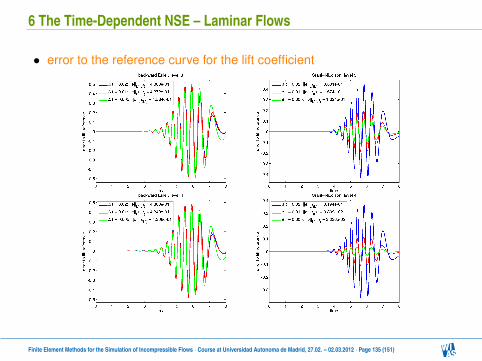
6 The Time-Dependent NSE – Laminar Flows
• error to the reference curve for the lift coefficient
Finite Element Methods for the Simulation of Incompressible Flows · Course at Universidad Autonoma de Madrid, 27.02. – 02.03.2012 · Page 135 (151)
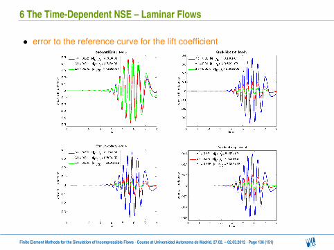
6 The Time-Dependent NSE – Laminar Flows
• error to the reference curve for the lift coefficient
Finite Element Methods for the Simulation of Incompressible Flows · Course at Universidad Autonoma de Madrid, 27.02. – 02.03.2012 · Page 136 (151)

6 The Time-Dependent NSE – Laminar Flows
• temporal evolution of lift coefficient
• BWE much to inaccurate (dissipative)
Finite Element Methods for the Simulation of Incompressible Flows · Course at Universidad Autonoma de Madrid, 27.02. – 02.03.2012 · Page 137 (151)

6 The Time-Dependent NSE – Laminar Flows
• temporal evolution of lift coefficient
• BWE much to inaccurate (dissipative)
Finite Element Methods for the Simulation of Incompressible Flows · Course at Universidad Autonoma de Madrid, 27.02. – 02.03.2012 · Page 137 (151)

6 The Time-Dependent NSE – Laminar Flows
• projection method motivation: schemes without need to solve (nonlinear) saddle point
problems survey in [1]
[1] Guermond, Minev, Shen, CMAME 195, 6011–6045, 2006
Finite Element Methods for the Simulation of Incompressible Flows · Course at Universidad Autonoma de Madrid, 27.02. – 02.03.2012 · Page 138 (151)

6 The Time-Dependent NSE – Laminar Flows
• idea: decoupled NSE to obtain separate equations for velocity andpressure approximation of time derivative given (q-step scheme)
∂tu(tn+1)≈1∆t
(τqun+1 +
q−1
∑i=0
τ jun− j
),
q
∑i=0
τ j = 0
equation for intermediate velocity: given p or ∇p
1∆t
(τqun+1 +
q−1
∑i=0
τ jun− j
)−ν∆u+(u ·∇)u = f−∇p in (0,T ]×Ω
correction step for divergence-free velocity
1∆t
(τqun+1− τqun+1)+∇ϕ (u)+∇p = ∇p in (0,T ]×Ω,
∇ ·u = 0 in [0,T ]×Ω
ϕ(·) – given function
Finite Element Methods for the Simulation of Incompressible Flows · Course at Universidad Autonoma de Madrid, 27.02. – 02.03.2012 · Page 139 (151)
6 The Time-Dependent NSE – Laminar Flows
• velocity computed in projection step is L2(Ω) projection of un+1 into
Hdiv(Ω) =
v ∈ L2(Ω), ∇ ·v ∈ L2(Ω) : ∇ ·v = 0 and v ·n = 0 on Γ
Finite Element Methods for the Simulation of Incompressible Flows · Course at Universidad Autonoma de Madrid, 27.02. – 02.03.2012 · Page 140 (151)
6 The Time-Dependent NSE – Laminar Flows
• non-incremental pressure-correction scheme p = 0, ϕ (·) = 0 proposed in [1,2] with backward Euler
• intermediate velocity
un+1 +∆tn+1 (−ν∆un+1 +(un ·∇)un+1) = un +∆tn+1fn+1 in Ω
with un+1 = 0 on Γ
• projection step
un+1 +∆tn+1∇pn+1 = un+1 in Ω,
∇ ·un+1 = 0 in Ω,
un+1 ·n = 0 on Γ
[1] Chorin, Math. Comp. 22, 745–762, 1968
[2] Temam, Arch. Rational Mech. Anal. 33, 377–385, 1969
Finite Element Methods for the Simulation of Incompressible Flows · Course at Universidad Autonoma de Madrid, 27.02. – 02.03.2012 · Page 141 (151)
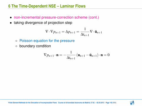
6 The Time-Dependent NSE – Laminar Flows
• non-incremental pressure-correction scheme (cont.)• taking divergence of projection step
∇ ·∇pn+1 = ∆pn+1 =1
∆tn+1∇ · un+1
Poisson equation for the pressure boundary condition
∇pn+1 ·n =− 1∆tn+1
(un+1− un+1) ·n = 0
• error estimates: (u, p) result of projection step
‖p− p‖l∞(0,T ;L2(Ω)) +‖u− u‖l∞(0,T ;H1(Ω)) ≤C (u, p,T )∆t1/2
if in addition domain has regularity property
‖u−u‖l∞(0,T ;L2(Ω)) +‖u− u‖l∞(0,T ;L2(Ω)) ≤C (u, p,T )∆t
Finite Element Methods for the Simulation of Incompressible Flows · Course at Universidad Autonoma de Madrid, 27.02. – 02.03.2012 · Page 142 (151)
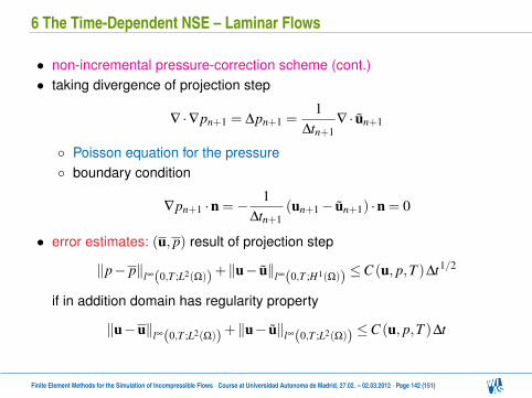
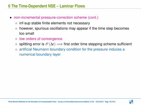
6 The Time-Dependent NSE – Laminar Flows
• non-incremental pressure-correction scheme (cont.) inf-sup stable finite elements not necessary however, spurious oscillations may appear if the time step becomes
too small low orders of convergence splitting error is O (∆t) =⇒ first order time stepping scheme sufficient artificial Neumann boundary condition for the pressure induces a
numerical boundary layer
Finite Element Methods for the Simulation of Incompressible Flows · Course at Universidad Autonoma de Madrid, 27.02. – 02.03.2012 · Page 143 (151)

6 The Time-Dependent NSE – Laminar Flows
• standard incremental pressure-correction scheme p = pn, ϕ (·) = 0 with BDF2
• intermediate velocity
3un+1 +2∆t (−ν∆un+1 +(un ·∇)un+1)
= 4un−un−1 +2∆t (fn+1−∇pn) in Ω,
with un+1 = 0 on Γ
• projection step
3un+1 +2∆t∇(pn+1− pn) = 3un+1 in Ω,
∇ ·un+1 = 0 in Ω,
un+1 ·n = 0 on Γ
Finite Element Methods for the Simulation of Incompressible Flows · Course at Universidad Autonoma de Madrid, 27.02. – 02.03.2012 · Page 144 (151)
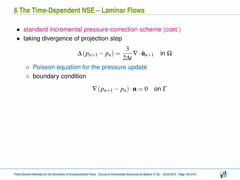
6 The Time-Dependent NSE – Laminar Flows
• standard incremental pressure-correction scheme (cont.)• taking divergence of projection step
∆(pn+1− pn) =3
2∆t∇ · un+1 in Ω
Poisson equation for the pressure update boundary condition
∇(pn+1− pn) ·n = 0 on Γ
• error estimates, with appropriate initial step, (u, p) result of projectionstep
‖p− p‖l∞(0,T ;L2(Ω)) +‖u− u‖l∞(0,T ;H1(Ω)) ≤C (u, p,T )∆t
if in addition domain has regularity property
‖u−u‖l∞(0,T ;L2(Ω)) +‖u− u‖l2(0,T ;L2(Ω)) ≤C (u, p,T )∆t2
Finite Element Methods for the Simulation of Incompressible Flows · Course at Universidad Autonoma de Madrid, 27.02. – 02.03.2012 · Page 145 (151)

6 The Time-Dependent NSE – Laminar Flows
• standard incremental pressure-correction scheme (cont.) similar estimates for Crank–Nicolson scheme splitting error is O
(∆t2)=⇒ second order time stepping scheme
sufficient artificial Neumann boundary condition for the pressure induces a
numerical boundary layer
Finite Element Methods for the Simulation of Incompressible Flows · Course at Universidad Autonoma de Madrid, 27.02. – 02.03.2012 · Page 146 (151)
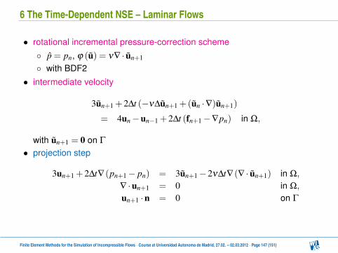
6 The Time-Dependent NSE – Laminar Flows
• rotational incremental pressure-correction scheme p = pn, ϕ (u) = ν∇ · un+1
with BDF2• intermediate velocity
3un+1 +2∆t (−ν∆un+1 +(un ·∇)un+1)
= 4un−un−1 +2∆t (fn+1−∇pn) in Ω,
with un+1 = 0 on Γ
• projection step
3un+1 +2∆t∇(pn+1− pn) = 3un+1−2ν∆t∇(∇ · un+1) in Ω,
∇ ·un+1 = 0 in Ω,
un+1 ·n = 0 on Γ
Finite Element Methods for the Simulation of Incompressible Flows · Course at Universidad Autonoma de Madrid, 27.02. – 02.03.2012 · Page 147 (151)
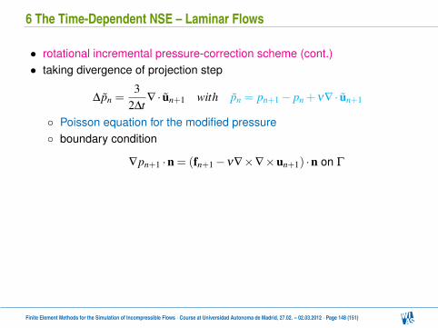
6 The Time-Dependent NSE – Laminar Flows
• rotational incremental pressure-correction scheme (cont.)• taking divergence of projection step
∆pn =3
2∆t∇ · un+1 with pn = pn+1− pn +ν∇ · un+1
Poisson equation for the modified pressure boundary condition
∇pn+1 ·n = (fn+1−ν∇×∇×un+1) ·n on Γ
• error estimates, with appropriate initial step, (u, p) result of projectionstep
‖p− p‖l2(0,T ;L2(Ω))+‖u− u‖l2(0,T ;H1(Ω))+‖u−u‖l2(0,T ;H1(Ω))≤C (u, p,T )∆t3/2
if in addition domain has regularity property
‖u−u‖l2(0,T ;L2(Ω)) +‖u− u‖l2(0,T ;L2(Ω)) ≤C (u, p,T )∆t2
Finite Element Methods for the Simulation of Incompressible Flows · Course at Universidad Autonoma de Madrid, 27.02. – 02.03.2012 · Page 148 (151)
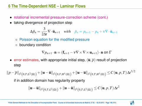
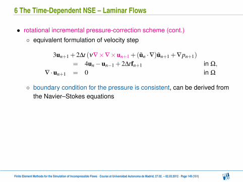
6 The Time-Dependent NSE – Laminar Flows
• rotational incremental pressure-correction scheme (cont.) equivalent formulation of velocity step
3un+1 +2∆t (ν∇×∇×un+1 +(un ·∇)un+1 +∇pn+1)
= 4un−un−1 +2∆tfn+1 in Ω,
∇ ·un+1 = 0 in Ω
boundary condition for the pressure is consistent, can be derived fromthe Navier–Stokes equations
Finite Element Methods for the Simulation of Incompressible Flows · Course at Universidad Autonoma de Madrid, 27.02. – 02.03.2012 · Page 149 (151)
6 The Time-Dependent NSE – Laminar Flows
• only un+1 needed in implementation• first experience with non-incremental and standard incremental scheme:
very inaccurate at boundaries (bad drag and lift coefficients)
Finite Element Methods for the Simulation of Incompressible Flows · Course at Universidad Autonoma de Madrid, 27.02. – 02.03.2012 · Page 150 (151)
Thank you for your attention !
http://www.wias-berlin.de/people/john/
Finite Element Methods for the Simulation of Incompressible Flows · Course at Universidad Autonoma de Madrid, 27.02. – 02.03.2012 · Page 151 (151)