Finite Element Methods

for the Incompressible Navier-Stokes Equations

Rolf Rannacher ∗

Institute of Applied Mathematics

University of Heidelberg

INF 293/294, D-69120 Heidelberg, Germany

E-Mail: rannacher@iwr.uni-heidelberg.de

URL: http://gaia.iwr.uni-heidelberg.de

Version of August 11, 1999

Abstract

These notes are based on lectures given in a Short Course on Theo-retical and Numerical Fluid Mechanics in Vancouver, British Columbia,Canada, July 27-28, 1996, and at several other places since then. Theyprovide an introduction to recent developments in the numerical solu-tion of the Navier-Stokes equations by the finite element method. Thematerial is presented in eight sections:

1. Introduction: Computational aspects of laminar flows2. Models of viscous flow3. Spatial discretization by finite elements4. Time discretization and linearization5. Solution of algebraic systems6. A review of theoretical analysis7. Error control and mesh adaptation8. Extension to weakly compressible flows

Theoretical analysis is offered to support the construction of numericalmethods, and often computational examples are used to illustrate the-oretical results. The variational setting of the finite element Galerkinmethod provides the theoretical framework. The goal is to guide thedevelopment of more efficient and accurate numerical tools for com-puting viscous flows. A number of open theoretical problems will beformulated, and many references are made to the relevant literature.

∗The author acknowledges the support by the German Research Association (DFG)through the SFB 359 “Reactive Flow, Diffusion and Transport” at the University of Heidel-berg, Im Neuenheimer Feld 294, D-69120 Heidelberg, Germany.

1

1 Introduction

In the following sections, we will discuss a computational methodology for sim-ulating viscous incompressible laminar flows. The description of the numericalalgorithms will be accompanied by a heoretical analysis so far as it is relevantto understanding the performance of the method. In this sense, these notesare meant as a contribution of Mathematics to “CFD” (Computational FluidDynamics).

Figure 1: Nonstationary flow around “CFD” for Re = 500 , driven by rotation ofthe outer circle and visualized by temperature isolines; from Turek [98].

The established model for viscous Newtonian incompressible flow is the thesystem of Navier-Stokes equations,

∂tv − ν∆v + v·∇v + ∇p = f, ∇·v = 0, (1)

in some region Ω × (0, T ) with appropriate initial and boundary conditions.We concentrate on “laminar” flows, i.e., on flows with Reynolds number in therange 1 ≤ Re ≤ 105 , where Re ∼ vl/ν . The numerical solution of this systeminvolves several typical difficulties:

• Complicated flow structure ⇒ fine meshes!

• Re ≫ 1 ⇒ locally refined and anisotropic meshes in boundary layers!

• Dominant nonlinear effects ⇒ stability problems!

• Constraint ∇·v = 0 ⇒ implicit solution!

• Sensitive quantities ⇒ solution-adapted meshes!

2

Accurate flow prediction requires the use of large computer power, particularlyfor the extension from 2D to 3D, from stationary to nonstationary flows, andfrom qualitative results to quantitatively accurate results. The key goals inthe developing tools for computing laminar flows are:

• fast (nonstationary calculations in minutes or hours),

• cheap (simulations on workstations),

• flexible (general purpose solver),

• accurate (adaptive error control).

1.1 Solution method

The method of choice in these notes is the “Finite Element Method” (FEM) forcomputing the primitive variables v (velocity) and p (pressure). This specialGalerkin method is based an a variational formulation of the Navier-Stokesproblem in appropriate function spaces, and determines “discrete” approxi-mations in certain finite dimensional subspaces (“trial spaces”) consisting ofpiecewise polynomial functions. By this approach the discretization inheritsmost of the rich structure of the continuous problem, which, on the one handprovides a high computational flexibility and on the other hand facilitates a rig-orous mathematical error analysis. These are the main aspects which make theFEM increasingly attractive in CFD. For completeness, we briefly commenton the essential features of the main competitors of the FEM:

• Finite difference methods (FDM): Approximation of the Navier-Stokes equations in their “strong” form by finite differences:+ easy implementation,− problems along curved boundaries,− difficult stability and convergence analysis,− mesh adaptation difficult.

• Finite volume methods (FVM): Approximation of the Navier-Stokesequations as a system of (cell-wise) conservation equations:+ based on “physical” conservation properties,− problems on unstructured meshes,− difficult stability and convergence analysis,− only heuristic mesh adaptation.

• Spectral Galerkin methods: Approximation of the Navier-Stokesequations in their variational form by a Galerkin method with “high-order” polynomial trial functions:+ high accuracy,− treatment of complex domains difficult,− mesh and order (hp)-adaptation difficult.

3

This brief classification must be superficial and is based on personal taste. Thedetails are the subject of much controversial discussion concerning the prosand cons of the various methods and their variants. However, this conflictis partially resolved in many cases, as the differences between the methods,particularly between FEM and FVM, often disappear on general meshes. Infact, some of the FVMs can be interpreted as variants of certain “mixed”FEMs.

1.2 Examples of computable viscous flows

Below, we give some examples of flows which can be computed by the methodsdescribed in these notes. More examples including movies of nonstationaryflows can be seen on our homepage: http://gaia.iwr.uni-heidelberg.de/.Some of the computer codes are available for research purposes:

• FEATFLOW Code (FORTRAN 77) by S. Turek [96], [97]:http://gaia.iwr.uni-heidelberg.de/~featflow/.

• deal.II Code (C++) by W. Bangerth and G. Kanschat [5]:http://gaia.iwr.uni-heidelberg.de/~deal/.

A collection of experimental photographs of such “computable” flows can befound in Van Dyke’s book “An Album of Fluid Motion” [99]. In the following,we present some examples of viscous flows which have been computed by themethodology described in these notes. Most of these results emerged as sideproducts in the course of developing the numerical solvers and testing them forstandard benchmark problems. All computations were done on normal workstations.

Example 1. Cavity flow: The first example is stationary and nonstationaryflow in a cavity driven by flow along the upper boundary (“driven cavity”).

Figure 2: Stationary driven cavity flow in 2D for Re = 1, 1000, 9000 (from left toright); for Re > 10000 the flow becomes nonstationary; from Turek [98].

4

Figure 3: Simulation of nonstationary 3D driven cavity flow for Re = 100 ; fromOswald [66].

Example 2. Vortex shedding: The second example is nonstationary flowaround a circular cylinder (“von Karman vortex street”)

Figure 4: Von Karman vortex street; experiment with Re = 105 (left; from VanDyke [99]), and 2D computation with Re = 100 (right; from Turek [98]).

Figure 5: 3D simulation of vortex shedding behind a cylinder for Re = 100 , coarsegrid and flow visualized by particle tracing; from Oswald [66].

5

Example 3. Leapfrogging of vortex rings: Two successive puffs of fluidare injected through a hole and develop into vortex rings dancing around eachother. The second ring travels faster in the induced wake of the first and slipsthrough it. Then the first ring slips through the second, and so on.

Figure 6: Leapfrogging of two vortex rings; experiment for Re ≈ 1600 (left;from Van Dyke [99]) and 2D computation for Re ≈ 500 (right; from [46]).

1.2.1 Extensions beyond standard Navier-Stokes flow

The numerical methodology described in these notes has primarily been de-veloped for computing viscous incompressible Newtonian flows. However, ex-tensions are possible in several directions. These include flows in regions withmoving boundaries, as for example pipe flow driven by rotating propellers, andflow of non-Newtonian fluids modelled by a simple power-law rule. The exten-sion to certain low-speed compressible flows will be discussed in more detailbelow in Section 8.

6

1) Flow regions with moving boundaries

Figure 7: Velocity plot of 2D flow in a box driven by a rotating cross, computed bya “virtual boundary” technique; from Turek [97].

2) Flow of a non-Newtonian fluid

Figure 8: Computation of the flow of a non-Newtonian fluid around a circularobstacle in a 2D channel (“power-law” ν = ν(1 + |D(v)|)−1 ): stationary flow inthe Newtonian case (left) and nonstationary flow in the non-Newtonian case (right),both for the same Reynolds number Re = 20; from Turek [98].

3) Low-Mach-number compressible flow

Figure 9: Computation of compressible flow in a chemical flow reactor: flow con-

figuration and mass fraction of excited H(ν=1)2 computed on a locally refined mesh;

from Waguet [103] and [10].

7

2 Models of viscous flow

The mathematical model for describing viscous (Newtonian) flows is the systemof Navier–Stokes equations, which are the equations of conservation of mass,momentum and energy:

∂tρ+ ∇·[ρv] = 0 , (1)

∂t(ρv) + ρv·∇v −∇·[µ∇v + 13µ∇·vI] + ∇ptot = ρf , (2)

∂t(cpρT ) + cpρv·∇T −∇·[λ∇T ] = h . (3)

Here, v is the velocity, ρ the density, ptot the (total) pressure, and T thetemperature of the fluid occupying a two- or three-dimensional region Ω . Theparameters µ > 0 (dynamic viscosity), cp > 0 (heat capacity) and λ > 0(heat conductivity) characterize the properties of the fluid. The volume forcef and the heat source h are explicitly given. Since we only consider low-speed flows, the influence of stress and hydrodynamic pressure in the energyequation can be neglected. In temperature-driven flows, h may implicitlydepend on the temperature and further quantities describing heat release, asfor example by chemical reactions. Such “weakly compressible” flows will bebriefly considered at the end of these notes in Section 8. Here, the fluid isassumed to be incompressible and the density to be homogeneous, ρ ≡ ρ0 =const. , so that (1) reduces to the incompressibility constraint

∇·v = 0 . (4)

In this model, we consider as the primal unknowns the velocity v , the pressurep = ptot , and the temperature T . For most parts of the discussion, the flowis assumed to be isothermal, so that the energy equation decouples from themomentum and continuity equations, and the temperature only enters throughthe viscosity parameter. The system is closed by imposing appropriate initialand boundary conditions for the flow variables

v|t=0 = v0, v|Γrigid= 0 , v|Γin

= vin , (µ∂nv + pn)|Γout= 0 , (5)

and corresponding ones for the temperature, where Γrigid, Γin, Γout are therigid part, the inflow part and the outflow part of the boundary ∂Ω , respec-tively. The role of the natural outflow boundary condition on Γout will beexplained in more detail below.

In the isothermal case, assuming for simplicity that ρ0 = 1 , the Navier-Stokes system can be written in short as

∂tv + v·∇v − ν∆v + ∇p = f , ∇·v = 0 , (6)

with the kinematic viscosity parameter ν = µ/ρ0 . In this formulation thedomain Ω may be taken two- or three-dimensional according to the particularrequirements of the simulation. In our examples, we shall mostly refer to the

8

two-dimensional case. Through a scaling transformation this problem is madedimensionless, with the Reynolds Number Re = UL/ν as the characteristicparameter, where U is the reference velocity (e.g., U ≈ max |vin| ) and L thecharacteristic length (e.g., L ≈ diam(Ω) ), of the problem.

As common in the mathematical literature, we assume that U = 1 andL = 1 and consider ν := 1/Re as a dimensionless parameter characterizing insome sense the “complexity” of the flow problem. Then, the length of the timeinterval over which the solution develops its characteristic features is T ≈ 1/ν ,and the relevant scale of its spatial structures is δx ≈ √

ν (width of boundarylayers). This has to be kept in mind when the right spatial mesh size h andthe time step k is chosen for a numerical simulation which is supposed toresolve all structures of the flow; for a more detailed discussion of the issue ofreliable transient flow calculation see [54].

2.1 Variational formulation

The finite element discretization of the Navier-Stokes problem (6) is based onits variational formulation. To this end, we use the following sub-spaces of theusual Lebesgue function space L2(Ω) of square-integrable functions on Ω :

L20(Ω) =

ϕ ∈ L2(Ω) : (v, 1) = 0

,

H1(Ω) =v ∈ L2(Ω), ∂iv ∈ L2(Ω), 1 ≤ i ≤ d

,

H10 (Γ; Ω) =

v ∈ H1(Ω), v|Γ = 0

, Γ ⊂ ∂Ω,

and the corresponding inner products and norms

(u, v) =

∫

Ω

uv dx , ‖v‖ = (v, v)1/2 ,

‖∇v‖ = (∇v,∇v)1/2 , ‖v‖1 =(‖v‖2 + ‖∇v‖2

)1/2.

These are all spaces of R-valued functions. Spaces of Rd-valued functions

v = (v1, . . . , vn) are denoted by boldface-type, but no distinction is madein the notation of norms and inner products; thus H1

0(Γ; Ω) = H10 (Γ; Ω)d

has norm ‖v‖1 = (∑d

i=1 ‖vi‖21)

1/2 , etc. All the other notation is self-evident:∂tu = ∂u/∂t, ∂iu = ∂u/∂xi, ∂nv = n·∇v, ∂τ = τ ·∇v etc., where n and τ arethe normal and tangential unit vectors along the boundary ∂Ω .

The pressure p in the Navier-Stokes equations is uniquely (possibly up toa constant) determined by the velocity field v . This follows from the fact thatevery bounded functional F (·) on H1

0(Γ; Ω) which vanishes on the subspace

J1(Γ; Ω) = v ∈ H10(Γ; Ω), ∇·v = 0

can be expressed in the form F (ϕ) = (p,∇·ϕ) for some p ∈ L2(Ω) . Further,there holds the stability estimate (“inf-sup” stability)

infq∈L2(Ω)

sup

φ∈H10(Γ;Ω)

(q,∇·φ)

‖∇φ‖

≥ γ0 > 0 , (7)

9

where L2(Ω) has to be replaced by L20(Ω) in the case Γ = ∂Ω . For proofs

of these facts, one may consult the first parts of the books of Ladyshenskaya[58], Temam [88] and Girault/Raviart [29]. Finally, we introduce the notation

a(u, v) := ν(∇u,∇v) , n(u, v, w) := (u·∇v, w) , b(p, v) := −(p,∇·v),

and the abbreviations

H := H10(Γ; Ω), L := L2(Ω)

(L := L2

0(Ω) in the case Γ = ∂Ω),

where Γ = Γin∪Γrigid . Then, the variational formulation of the Navier-Stokesproblem (6), reads as follows: Find functions v(·, t) ∈ vin +H and p(·, t) ∈ L ,such that v|t=0 = v0 , and setting Γ := Γin ∪ Γrigid ,

(∂tv, ϕ) + a(v, ϕ) + n(v, v, ϕ) + b(p, v) = (f, ϕ) ∀ϕ ∈ H , (8)

(∇·v, χ) = 0 ∀χ ∈ L . (9)

It is well known that in two space dimensions the pure Dirichlet problem(8), (9), with Γout = ∅ , possesses a unique solution on any time interval[0, T ] , which is also a classical solution if the data of the problem are smoothenough. For small viscosity, i.e., large Reynolds numbers, this solution may beunstable. In three dimensions, the existence of a unique solution is known onlyfor sufficiently small data, e.g., ‖v0‖1 ≈ ν , or on sufficiently short intervals oftime, 0 ≤ t ≤ T , with T ≈ ν .

2.2 Regularity of solution

We collect some results concerning the regularity of the variational solutionof the Navier-Stokes problem which are relevant for the understanding of itsnumerical approximation. One obtains quantitative regularity bounds fromthe following sequence of differential identities

12dt‖v‖2 + ν‖∇v‖2 = (f, v),

12dt‖∇v‖2 + ν‖∆v‖2 = −(f,∆v) + (v·∇v,∆v),

12dt‖∂tv‖2 + ν‖∇∂tv‖2 = (∂tf, ∂tv) − (∂tv·∇v, ∂tv),

12dt‖∇∂tv‖2 + ν‖∆∂tv‖2 = −(∂tf,∆∂tv) + (∂tv·∇v,∆∂tv) + ... ,

12dt‖∂2

t v‖2 + ν‖∇∂2t v‖2 = (∂2

t f, ∂2t v) − (∂2

t v·∇v, ∂2t v) − ... ,

...

which are easily derived by standard energy arguments; see [40] and [41]. As-suming a bound on the Dirichlet norm of v ,

supt∈(0,T ]

‖∇v(t)‖ ≤M, (10)

the above estimates together with the usual elliptic regularity results im-ply that v is smooth on Ω for 0 < t ≤ T , if all the data and ∂Ω are

10

smooth. However, for the purposes of numerical analysis one needs regu-larity estimates which hold uniformly for t → 0 . To get such informa-tion from the above equations requires starting values for all the quantities‖v‖, ‖∇v‖, ‖∂tv‖, ‖∇∂tv‖, ‖∂2

t v‖ , etc., at t = 0 . However, there is a problemalready with ‖∇∂tv(0)‖ , as has been demonstrated in [41].

2.2.1 Compatibility conditions at t = 0

To investigate this phenomenon, let us assume that the solution v, p isuniformly smooth as t → 0 . Then, applying the divergence operator to theNavier-Stokes equations and letting t→ 0 implies:(i) in Ω :

∇·(∂tv + v·∇v) = ∇·(ν∆v −∇p) → ∇·(v0·∇v0) = −∆p0,

(ii) on ∂Ω :

∂tv + v·∇v = ν∆v −∇p → ∂tg|t=0 + v0·∇v0 = ν∆v0 −∇p0,

where g is the boundary data, v0 the initial velocity and p0 := limt→0 p(t)the “initial pressure”. Hence, in the limit t = 0 , we obtain an overdeterminedNeumann problem for the initial pressure:

∆p0 = −∇·(v0·∇v0) in Ω, (11)

∇p0|∂Ω = ν∆v0 − ∂tg|t=0 − v0·∇v0, (12)

including the compatibility condition

∂τp0|∂Ω = τ ·(ν∆v0 − ∂tg|t=0 − v0·∇v0), (13)

where τ is the tangent direction along ∂Ω . If this compatibility is violated,then limt→0‖∇3v(t)‖ + ‖∇∂tv(t)‖ = ∞ ; see [41]. We emphasize that (13)together with (11) is a global condition which in general cannot be verified forgiven data. Without (13) being satisfied the maximum degree of regularity isright in the middle of H2 and H3; see [78]. In view of the foregoing discus-sion, the natural regularity assumption for the nonstationary Navier-Stokesequations (without additional compatibility condition) is

v0 ∈ J1(Ω) ∩ H2(Ω) ⇒ supt∈(0,T ]

‖∇2v(t)‖ + ‖∂tv(t)‖

<∞. (14)

Example: Flow between two concentric spheres (“Taylor problem”)Let the inner sphere with radius rin be accelerated from rest v0 = 0 with aconstant acceleration ω , i.e., v|Γin

·(n, τθ, τφ)T = rin cos(θ)(0, 0, ωt)T (in polarcoordinates), while at the outer sphere, we set v|Γout

= 0 . Accordingly, theNeumann problem for the “initial pressure” takes the form

∆p0 = 0 in Ω, ∂np0|∂Ω = 0,

11

which implies that p0 ≡ const . However, this conflicts with the compatibilitycondition (13) which in this case reads

∂φp0|Γin

= −∂t(v0·nφ)t=0 = −rin cos(θ)ω 6= 0 .

In order to describe the “natural” regularity of the solution v(t), p(t) , ast → 0 , and as t → ∞ , in [41] a sequence of time-weighted a priori estimateshas been proven under the assumption (10) using the weight functions τ(t) =min(t, 1) and eαt , with fixed α > 0 :

τ(t)2n+m−2‖∇m∂nt v(t)‖ + ‖∇m−1∂nt p(t)‖

≤ K, (15)

and

e−αt∫ t

0

eαsτ(s)2n+m−2‖∇m∂nt v(t)‖2 + ‖∇m−1∂nt p(t)‖2

dt ≤ K, (16)

for any m ≥ 2, n ≥ 1 .

Open problem 2.1: Devise a way to construct for any given initial datav0 (e.g., fitted from experimental data) and any ǫ > 0 a smooth initial datav0 ∈ J1(Γ; Ω) , such that ‖v0 − v0‖1 ≤ ǫ , and the resulting solution of theNavier-Stokes equations satisfies the compatibility condition (13) at t = 0 .

2.3 Outflow boundary conditions

Numerical simulation of flow problems usually requires the truncation of aconceptionally unbounded flow region to a bounded computational domain,thereby introducing artificial boundaries, along which some kind of boundaryconditions are needed. The variational formulation (8), (9) does not containan explicit reference to any “outflow boundary condition”. Suppose that thesolution v ∈ vin +H, p ∈ L is sufficiently smooth. Then, integration by partson the terms

ν(∇v∇φ) − (p,∇·φ) =

∫

Γout

ν∂nv − pnφ do+ (−ν∆v + ∇p, φ)

12

yields the already mentioned “natural” condition on the outflow boundary

ν∂nv − pn = 0 on Γout. (17)

This condition has proven to be well suited in modeling (essentially) parallelflows, see, e.g., [46], Turek [93, 97]. It naturally occurs in the variationalformulation of the problem if one does not prescribe any boundary conditionfor the velocity at the outlet suggesting the name “do nothing” boundarycondition.

In the following, we present some experiences in choosing the boundaryconditions implicitly, through the choice of variational formulations of flowproblems used in finite element computations. To fix ideas, let us begin byconsidering a common test problem, that of calculating nonstationary flowpast an obstacle (here an inclined ellipse), situated in a rectangular channel.

Figure 10: The effect of the “do nothing” outflow boundary condition shown bypressure isolines for unsteady flow around an inclined ellipse at Re=500; from [46].

We impose the usual no-slip boundary conditions on the channel walls andon the surface of the ellipse, while a parabolic “Poiseuille” inflow profile isprescribed on the upstream boundary. We denote again by Γ that portion ofthe boundary on which Dirichlet conditions are imposed. At the downstreamboundary S = Γout , we decide to “do nothing” and leave the solution andthe test space free by choosing H = H1

0(Γ; Ω) and L = L2(Ω) . This resultsin the free-outflow condition (17). The results of computations based on (17)show a truly remarkable “transparency” of the downstream boundary when itis handled in this way; see Figure 10 where almost no effect of shortening thecomputational domain is seen.

13

2.3.1 Problems with the “do nothing” outflow condition

Although, the “do nothing” outflow boundary condition seems to yield verysatisfactory results, one should use it with care. For example, if the flow re-gion contains more than one outlet, like in flows through systems of pipes,undesirable effects may occur, since the “do nothing” condition contains asan additional hidden condition that the mean pressure is zero across the out-flow boundary. In fact integrating (17) over any component S of the out-flow boundary (a straight segment) and using the incompressibility constraint∇·v = 0 yields

∫

S

pn do = ν

∫

S

∂nv do = −ν∫

S

∂tv do = v(s2) − v(s1) = 0 .

Here si denote the end points of S at which v(si) = 0 , due to the imposedno-slip condition along Γ . Consequently, the mean pressure over S must bezero: ∫

S

p do = 0 . (18)

To illustrate this, let us consider low Reynolds number flow through a junctionin a system of pipes, again prescribing a Poiseuille inflow upstream. In Figure11, we show steady streamlines for computations based on the same variationalformulations as above, each with the same inflow, but with varying lengthsof pipe beyond the junction. Obviously, making one leg of the pipe longersignificantly changes the flow pattern. The explanation of this effect is that bythe property (18), in Figure 11 the pressure gradient is greater in the shorterof the two outflow sections, which explains why there is a greater flow throughthat section.

Figure 11: The effect of the “do nothing” outflow boundary condition shown bystreamline plots for flow through a bifurcating channel for Re = 20 ; from [46].

2.3.2 Modification of transport or diffusion model

The foregoing example suggests that one might consider formulating problemsmore generally, e.g., in terms of prescribed pressure drops or prescribed fluxes;we refer to [46] for a thorough development of the corresponding variationalformulations. Both choices of boundary conditions lead to well posed formu-lations of the problem. However, the situation is less satisfactory than in thecase of pure Dirichlet boundary conditions. Although the variational problem

14

looks well set in this situation, surprisingly there is a problem with its wellposedness. The related Dirichlet problem of the Navier-Stokes equations, sta-tionary as well as nonstationary, is well known to possess weak solutions (notnecessarily unique or stable) for any Reynolds number. The standard argu-ment for this result is based upon the “conservation property” (v·∇v, v) = 0of the nonlinear term, which is obtained by integration by parts and using∇·v = 0 . In the case of a “free” boundary this relation is replaced by

(v·∇v, v) = −12(n·v, v2)Γ, Γ = ∪iΓi, (19)

which generally does not allow to bound the energy in the system without apriori knowledge of what is an inflow and what is an outflow boundary. As aconsequence, in [46] the existence of a unique solution could be shown, evenin two space dimensions, only for sufficiently small data. Kracmar/Neustupa[57] have treated the case of general data by formulating the problem as avariational inequality including the energy bound as a constraint. This stillleaves the question open whether one can expect existence of solutions forthe original formulation with general data. A positive answer is suggested bynumerical tests which do not show any unexpected instability with the discreteanalogues of the formulation (8), (9) in the case of higher Reynolds numbers.

One may suspect that this theoretical difficulty can be avoided simply bychanging the variational formulation of the problem, i.e., using other varia-tional representations of the transport or diffusion terms. It has been sug-gested to replace in the momentum equation (8) the Dirichlet form (∇v,∇φ)by (D[v], D[φ]) , with D[v] = 1

2(∂ivj +∂jvi)

di,j=1 being the deformation tensor.

This change has no effect in the case of pure Dirichlet boundary conditionsas then the two forms coincide. But in using the “do nothing” approach thismodification leads to the outflow boundary condition

n·D[v] − pn = 0 on Γout,

which may result in a non-physical behavior of the flow. In the case of simplePoiseuille flow the streamlines are bent outward as shown in Figure 12.

Another possible modification is to enforce the conservation property onthe transport terms. Using the identity ∇(1

2|v|2) = v·(∇v)T , the transport

term can be written in the form

v·∇v = v·∇v − v·(∇v)T + 12∇|v|2.

This leads to a variational formulation in which (v·∇v, φ) is replaced by

b(v, v, φ) := (v·∇v, φ) − (φ·∇v, v), (20)

while the term 12|v|2 is absorbed into the pressure. An alternative form is

b(v, v, φ) := 12(v·∇v, φ) − 1

2(v·∇φ, v), (21)

15

which is legitimate because b(v, v, φ) = (v·∇v, φ) for v ∈ J1(Ω) . Notice thatin both cases b(w, φ, φ) = 0 for any w . The corresponding natural outflowboundary conditions are, for (20):

ν∂nv − pn = 0, (22)

with the so-called “Bernoulli pressure” p = p+ 12|v|2 , and for (21):

ν∂nv − 12|n·v|2n− pn = 0. (23)

Both modifications again result in a non-physical behavior across the outflowboundary; streamlines bent inward as shown in Figure 12. Hence, for physicalreasons, it seems to be necessary to stay with the original formulation (8), (9).For a detailed discussion of the boundary conditions, and for an extensive listof references, we refer the reader to Gresho [34] and Gresho and Sani [35].

Figure 12: The effect of using the deformation tensor formulation (top) or thesymmetrized transport formulations (middle) together with the “do nothing” outflowboundary condition compared to the correct Poiseuille flow (bottom); from [46].

Open Problem 2.2: Prove the existence of global smooth solutions (in 2D) forthe original variational Navier-Stokes equations with the “do nothing” outflowboundary condition for general data.

16

3 Spatial discretization by finite elements

In this section, we recall some basics about the spatial discretization of theincompressible Navier–Stokes equations by the finite element method. Theemphasis will be on those types of finite elements which are used in our codesfor solving two and three dimensional flow problems, stationary as well asnonstationary. For a general discussion of finite element methods for flowproblems, see to Girault/Raviart [29], Pironneau [68], and Gresho/Sani [35].

3.1 Basics of finite element discretization

We begin by a brief introduction to the basics of finite element discretization ofelliptic problems, e.g., the Poisson equation in a bounded domain Ω ⊂ R

d (d =2 or 3) with a polyhedral boundary ∂Ω ,

−ν∆u = f in Ω. (1)

We assume homogeneous Dirichlet and Neumann boundary conditions,

u|ΓD= 0, ∂nu|ΓN

= 0, (2)

along disjoint components ΓD and ΓN of ∂Ω , where ∂Ω = ΓD ∪ ΓN . Thestarting point is the variational formulation of this problem in the naturalsolution space H := H1

0 (ΓD; Ω) : Find u ∈ H satisfying

a(u, φ) := ν(∇u,∇φ) = (f, φ) ∀φ ∈ H. (3)

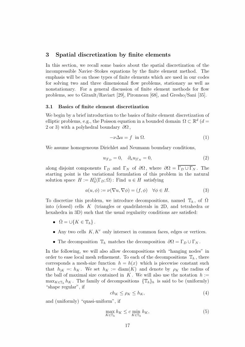
To discretize this problem, we introduce decompositions, named Th , of Ωinto (closed) cells K (triangles or quadrilaterals in 2D, and tetrahedra orhexahedra in 3D) such that the usual regularity conditions are satisfied:

• Ω = ∪K ∈ Th .

• Any two cells K,K ′ only intersect in common faces, edges or vertices.

• The decomposition Th matches the decomposition ∂Ω = ΓD ∪ ΓN .

In the following, we will also allow decompositions with “hanging nodes” inorder to ease local mesh refinement. To each of the decompositions Th , therecorresponds a mesh-size function h = h(x) which is piecewise constant suchthat h|K =: hK . We set hK := diam(K) and denote by ρK the radius ofthe ball of maximal size contained in K . We will also use the notation h :=maxK∈Th

hK . The family of decompositions Thh is said to be (uniformly)“shape regular”, if

chK ≤ ρK ≤ hK , (4)

and (uniformly) “quasi-uniform”, if

maxK∈Th

hK ≤ c minK∈Th

hK , (5)

17

with some constants c independent of h ; see Girault/Raviart [29] or Bren-ner/Scott [19] for more details of these properties. In the following, we will gen-erally assume shape-regularity (unless something else is said). Quasi-uniformityis usually not required. Examples of admissible meshes are shown below.

K

h

@@

@@

@@

@@

@@

@@

K

h

Figure 13: Regular finite element meshes (triangular and quadrilateral)

On the decompositions Th , we consider “finite element spaces” Hh ⊂ Hdefined by

Hh := vh ∈ H, vh|K ∈ P (K), K ∈ Th,where P (K) are certain spaces of elementary functions on the cells K . Inthe simplest case, P (K) are polynomial spaces, P (K) = Pr(K) for somedegree r ≥ 1 . On general quadrilateral or hexahedral cells, we have to workwith “parametric” elements, i.e., the local shape functions are constructed byusing transformations ψK : K → K between the “physical” cell K and afixed “reference unit-cell” K by vh|K(ψK(·)) ∈ Pr(K) . This construction isnecessary in general in order to preserve “conformity” (i.e., global continuity) ofthe cell-wise defined functions vh ∈ Hh . For example, the use of bilinear shapefunctions φ ∈ span1, x1, x2, x1x2 on a quadrilateral mesh in 2D employslikewise bilinear transformations ψK : K → K . We will see more examples ofconcrete finite element spaces below.

In a finite element discretization, “consistency” is expressed in terms oflocal approximation properties of the shape functions used. For example, in thecase of a second-order approximation using linear or d-linear shape functions,there holds locally on each cell K :

‖v − Ihv‖K + hK‖∇(v − Ihv)‖K ≤ cIh2K‖∇2v‖K , (6)

and on each cell surface ∂K :

‖v − Ihv‖∂K + hK‖∂n(v − Ihv)‖∂K ≤ cIh3/2K ‖∇2v‖K, (7)

where Ihv ∈ Hh is the natural “nodal interpolation” of a function v ∈H ∩ H2(Ω) , i.e., Ihv coincides with v with respect to certain “nodal func-tionals” (e.g., point values at vertices, mean values on edges or faces, etc.).The “interpolation constant” is usually of size cI ∼ 0.1−1 , depending on theshape of the cell K.

18

With the foregoing notation the discrete scheme reads as follows: Finduh ∈ Hh satisfying

a(uh, φh) = (f, φh) ∀φh ∈ Hh. (8)

Combining the two equations (3) and (8) yields the relation

a(u− uh, φh) = 0, φh ∈ Hh, (9)

which means that the error e := u − uh is “orthogonal” to the subspaceHh with respect to the bilinear form a(·, ·) . This essential feature of thefinite element Galerkin scheme immediately implies the “best approximation”property

‖∇e‖ = minφh∈Hh

‖∇(u− φh)‖. (10)

In virtue of the interpolation estimate (6), we obtain the (global) a prioriconvergence estimate

‖∇e‖ ≤ cI h‖∇2u‖ ≤ cIcS h ‖f‖, (11)

provided that the solution is sufficiently regular, i.e., u ∈ H2(Ω), satisfyingthe a priori bound

‖∇2v‖ ≤ cS‖f‖. (12)

In the above model, this is the case if the polygonal domain Ω is convex.In case of reduced regularity of u due to reentrant corners, the order in theestimate is correspondingly reduced. In the case of approximation by higher-order polynomials, r ≥ 2 , and higher order of regularity of u , the estimate(11) shows a correspondingly increased power of h. The order of h in the“energy-error” estimate (11) can be improved by shifting to the L2-norm. Thisis done by employing a duality argument (“Aubin-Nitsche trick”); see, e.g.,Brenner/Scott [19]. Let z ∈ H be the solution of the auxiliary problem

−ν∆z = ‖e‖−1e in Ω, z = 0 on ∂Ω, (13)

satisfying an a priori bound ‖∇2z‖ ≤ cS . Then, there holds

‖e‖ = (e,−ν∆z) = a(e, z) = a(e, z − Ihz) ≤ cIcSh‖∇e‖, (14)

and we conclude the improved a priori L2-error estimate

‖e‖ ≤ c2Ic2Sh

2‖f‖ . (15)

In order to convert the problems (8) into a form which is amenable to prac-tical computation, we introduce the nodal basis φ1

h, . . . , φNh , N = dimHh ,

of the space Hh , defined by φih(aj) = δij , i, j = 1, . . . , N , where aj are thenodal points (e.g., the vertices) of the mesh. Then, setting

uh =

N∑

i=1

xiφih,

19

problem (8) is equivalent to the linear algebraic system

Ax = b , (16)

for the “nodal value” vector x = (xi)Ni=1 . Here, the “stiffness matrix” A and

the “load vector” b are defined by

A :=(a(φih, φ

jh)

)Ni,j=1

, b :=((f, φih)

)Ni=1

.

In the case of variable coefficients and force the integrals have to be computedby using integration formulas; in our implementations usually Gaussian formu-las are used. For the pure diffusion problem the stiffness matrix A is symmet-ric and positive definite. Its condition number behaves like κ(A) = O(h−2) ,where the exponent -2 is determined by the order of the differential operator∆ (it is independent of the spatial dimension and the polynomial degree ofthe finite elements used).

Below, we show a sequence of hexahedral 3D meshes used for computingthe “puff-puff flow” mentioned in the Introduction; observe the successivelyrefined approximation of the curved boundary.

Figure 14: Sequence of successively refined hexahedral meshes for computing the“puff-puff” flow in 3D.

3.2 Stokes elements

We consider the stationary Navier-Stokes problem as specified in Section 2.In setting up a finite element model of the Navier-Stokes problem, one startsfrom the variational formulation of the problem: Find v ∈ vin+H and p ∈ L ,such that

a(v, ϕ) + n(v, v, ϕ) + b(p, φ) = (f, ϕ) ∀ φ ∈ H, (17)

b(χ, v) = 0 ∀ χ ∈ L. (18)

The choice of the function spaces H ⊂ H1(Ω)) and L ⊂ L2(Ω) depends on thespecific boundary conditions imposed in the problem to be solved. On a finiteelement mesh Th on Ω with cell width h , one defines spaces of “discrete”trial and test functions,

Hh “⊂”H, Lh ⊂ L.

20

The discrete analogues of (19), (20) then read as follows: Find vh ∈ vinh + Hh

and ph ∈ Lh , such that

ah(vh, ϕh) + nh(vh, vh, φh) + bh(ph, φh) = (f, ϕh) ∀ φh ∈ Hh, (19)

bh(χh, vh) = 0 ∀ χh ∈ Lh, (20)

where vinh is a suitable approximation of the inflow data vin. The notationHh“⊂”H indicates that in this discretization the spaces Hh may be “noncon-forming”, i.e., the discrete velocities vh are continuous across the interelementboundaries and zero along the rigid boundaries only in an approximate sense;in this case the discrete forms ah(·, ·) , bh(·, ·) , nh(·, ·, ·) and the discrete “en-ergy norm” ‖∇ · ‖h are defined in the piecewise sense,

ah(φ, ψ) :=∑

K∈Th

ν(∇φ,∇ψ)K , bh(χ, φ) :=∑

K∈Th

(χ,∇·φ)K ,

nh(φ, ψ, ξ) :=∑

K∈Th

(φ·∇ψ, ξ)K , ‖∇φ‖h :=( ∑

K∈Th

‖∇φ‖2K

)1/2

.

In order that (19), (20) is a stable approximation to (17), (18), as h→ 0 , it iscrucial that the spaces Hh×Lh satisfy a compatibility condition, the so-called“inf–sup” or “Babuska-Brezzi” condition,

infqh∈Lh

sup

wh∈Hh

bh(qh, wh)

‖qh‖ ‖∇wh‖h

≥ γ > 0 . (21)

Here, the constant γ is required to be independent of h . This ensures thatthe problems (19), (20) possess solutions which are uniquely determined inHh×Lh and stable. Further, for the errors ev := v − vh and ep := p − ph ,there hold a priori estimates of the form

‖∇ev‖h + ‖ep‖ ≤ ch‖∇2v‖ + ‖∇p‖

. (22)

A rigorous convergence analysis of spatial discretization of the Navier-Stokesproblem can be found in Girault/Raviart [29] and in [41, 43].

3.2.1 Examples of Stokes elements

Many stable pairs of finite element spaces Hh, Lh have been proposed in theliterature (see, e.g., Girault/Raviart [29], Hughes et al. [49] and [77]). Below,two particularly simple examples of quadrilateral elements will be describedwhich have satisfactory approximation properties and are applicable in twoas well as in three space dimensions. They can be made robust against meshdegeneration (large aspect ratios) and they admit the application of efficientmultigrid solvers. We note that, from the point of view of accuracy, in ourcontext quadrilateral (hexahedral) elements are to be preferred over triangu-lar (tetrahedral) elements because of their superior approximation properties.

21

Both types of elements may be used in the spatial discretization underlyingthe discussions in the following sections.

1) The nonconforming “rotated” d-linear Q1/P0 Stokes elementThe first example is the natural quadrilateral analogue of the well-known tri-angular nonconforming finite element of Crouzeix/Raviart (see [29]). It wasintroduced and analyzed in [77] and its two- as well as three-dimensional ver-sions have been implemented in state-of-the-art Navier-Stokes codes (see Turek[93, 96], Schreiber/Turek [83], and Oswald [66]. In two space dimensions, thisnonconforming element uses piecewise ”rotated” bi-linear (reference) shapefunctions for the velocities, spanned by 1, x, y, x2 − y2 , and piecewise con-stant pressures. As nodal values one may take the mean values of the velocityvector over the element edges (or, alternatively, its point values at the mid-points of sides) and the mean values of the pressure over the elements. For theprecise definition of this element we introduce the set ∂Th of all (d− 1)-facesS of the elements K ∈ Th . We set

Q1(K) =q ψ−1

T : q ∈ span1, x1, x2i − x2

i+1, i = 1, ..., d.

The corresponding finite element spaces are

Hh :=

vh ∈ L2(Ω)d : vh|K ∈ Q1(K)d, K ∈ Th ,FS(vh|K) = FS(vh|K ′), S ⊂ ∂K ∩ ∂K ′, FS(vh) = 0, S ⊂ Γ

,

Lh :=qh ∈ L : qh|K ∈ P0(K), K ∈ Th

,

with the nodal functionals

FS(vh) = |S|−1

∫

S

vh do , FK(ph) = |K|−1

∫

K

ph dx .

d e

dd

d

DDDDDDD

1|K|

∫Kphdx

1|Γ|

∫Γvhds

r

r

r

r

r

r r

1|K|

∫Kphdx

1|Γ|

∫Γvhds

Clearly, the spaces Hh are non-conforming, Hh 6⊂H1(Ω)d . For the pairHh, Lh the discrete “inf-sup” stability condition (21) is known to be satisfiedon fairly general meshes; see [77] and [13]. For illustration, we recall from [13]the essential steps of the argument.

Proof of the “inf-sup” stability estimate (21): Using the continuous “inf-sup”estimate (7), we conclude for an arbitrary ph ∈ Lh that

γ0‖ph‖ ≤ supφ∈H

|bh(ph, φ)|‖∇φ‖ ≤ sup

rhφ∈Hh

|bh(ph, rhφ)|‖∇rhφ‖

supφ∈H

‖∇rhφ‖‖∇φ‖ . (23)

22

where rhφ ∈ Hh is an approximation to φ ∈ H satisfying

bh(χh, φ− rhφ) = 0 ∀χh ∈ Lh , ‖∇rhφ‖ ≤ c∗‖∇φ‖ . (24)

These properties are realized for the Q1/P0 Stokes element by the naturalnodal interpolation defined by

∫

S

rhφ do =

∫

S

φ do ∀ S ∈ ∂T.

Then, the first relation in (24) is obvious, and the H1 stability follows from

‖∇rhφ‖2h =

∑

K∈Th

(rhφ, ∂nrhφ)∂K − (rhφ,∆rhφ)K

= (∇φ,∇rhφ)h +∑

K∈Th

(rhφ− φ, ∂nrhφ)∂K − (rhφ− φ,∆rhφ)K

.

The argument becomes particularly simple for parallelogram meshes. In thiscase ∂nrhφ|Γ ≡ const. and ∆rhφ|K ≡ 0 , such that the last sum vanishes. Thegeneral case requires a more involved estimation. Now, the desired “inf-sup”stability estimate follows with the constant γ = γ0/c∗ .

As discussed in [77], the stability and approximation properties of theQ1/P0 Stokes element depend very sensitively on the degree of deviation ofthe cells K from parallelogram shape. Stability and convergence deteriorateswith increasing cell aspect ratios. This defect can be cured by using a “non-parametric” version of the element where the reference space Q1(K) :=

q ∈

span1, ξ, η, ξ2 − η2

is defined for each element K independently with re-spect to the coordinate system (ξ, η) spanned by the directions connectingthe midpoints of sides of K . This approximation turns out to be robust withrespect to the shape of the elements K , and the convergence estimate (22)remains true. Below, we will relax this requirement even further by allowingthe elements to be stretched in one or more (in 3D) directions.

Finally, we mention an important feature of the Q1/P0 Stokes element (see[93]): It possesses a “divergence-free” nodal-basis, which allows the elimina-tion of the pressure from the problem resulting in a positive definite algebraicsystem for the velocity unknowns alone. The reduced algebraic system can besolved by specially adapted multigrid methods; see Turek [93].

2)The conforming d-linear Q1/Q1 Stokes element with pressure stabilizationThe second example uses continuous isoparametric d-linear shape functions forboth the velocity and the pressure approximations. The nodal values are justthe function values of the velocity and the pressure at the vertices of the mesh,making this approximation particularly attractive in three dimensions. With

Q1(K) =q ψ−1

T : q ∈ span1, xi, xixj , i, j = 1, . . . , d,

23

the corresponding finite element spaces are defined by

Hh =vh ∈ H1

0(Γ; Ω)d : vh|K ∈ Q1(K)d, K ∈ Th

,

Lh =qh ∈ H1(Ω) : qh|K ∈ Q1(K), K ∈ Th

,

with the nodal functionals ( a vertex of the mesh Th )

Fa(vh) = vh(a) , Fa(ph) = ph(a) .

t t

tt

DDDDDDD

K

vh(a), ph(a)

r r

r

rr

r

rr

K

vh(a), ph(a)

This combination of spaces, however, would be unstable, i.e., it would violatethe condition (21), if used together with the variational formulation (19), (20).In order to get a stable discretization, it was proposed by Hughes et al. [49],to add certain least squares terms in the continuity equation (20) (pressurestabilization method),

b(χh, vh) + ch(χh, ph) = gh(vh;χh), (25)

where

ch(χh, ph) =α

ν

∑

K∈Th

h2K(∇χh,∇ph)K ,

gh(vh;χh) =α

ν

∑

K∈Th

h2K(∇χh, f + ν∆vh − vh·∇vh)K .

The correction terms on the right hand side have the effect that this modi-fication is fully consistent, since the additional terms cancel out if the exactsolution v, p of problem (17), (18) is inserted. On regular meshes, one ob-tains a stable and consistent approximation of the Navier-Stokes problem (17),(18), for which a convergence estimate of form (22) holds true. The argumentfollows a slightly different track than that used above for the nonconformingQ1/P0 element; see [13].

Proof of the “inf-sup” stability estimate (21): From the continuous stabilityestimate (7) we conclude that

γ0‖ph‖ ≤ suprhφ∈Hh

|(ph,∇rhφ)|‖∇rhφ‖

supφ∈H

‖∇rhφ‖‖∇φ‖ + sup

φ∈H

|(∇ph, φ− rhφ)|‖∇φ‖ , (26)

24

where rhφ ∈ Hh is an approximation to φ ∈ H , satisfying

( ∑

K∈Th

h−2K ‖φ− rhφ‖2

K

)1/2

+ ‖∇rhφ‖ ≤ c∗‖∇φ‖ . (27)

The existence of such an approximation can be shown by employing an aver-aged nodal interpolation. From this, we obtain

γ‖ph‖ ≤ c∗ supφh∈Hh

|(ph,∇φh)|‖∇φh‖

+ c∗

( ∑

K∈Th

h2K‖∇ph‖2

K

)1/2

,

which yields the desired stability estimate with the constant γ = γ0/c∗ .

It was shown in Hughes et al. [49], and later on in a series of mathematicalpapers (see, e.g., Brezzi/Pikaranta [21], and the literature cited therein) inthe context of a more general analysis of such stabilization methods, that thiskind of discretization is numerically stable and of optimal order convergent formany relevant pairs of spaces Hh×Lh .

The stabilized Q1/Q1 Stokes element has several important features: Withthe same number of degrees of freedom it is more accurate than its triangularanalogue (and also slightly more accurate than its nonconforming analoguedescribed above). Furthermore, it has a very simple data structure due to theuse of the same type of nodal values for velocities and pressure which allowsfor an efficient vectorization of solution processes. Thanks to the stabilizationterm in the continuity equation, standard multigrid techniques can be usedfor solving the algebraic systems with good efficiency (see the discussion inSection 5 below).

We note that the triangular analogue of this element is closely related(indeed almost algebraically equivalent) to the “inf-sup” stable MINI–element(see Brezzi/Fortin [20]) which is based on the standard Q1/Q1-element andstability is achieved by augmenting the velocity space by local cubic bubblefunctions.

The stabilized Q1/Q1-Stokes element has been implemented in several 2Dand 3D Navier-Stokes codes (see, e.g., Harig [38], Becker [7], and Braack [17]).However, it was already reported in Harig [38] that the convergence propertiesof this element sensitively depend on the parameter α and may deteriorate onstrongly stretched meshes. We will come back to this point below.

3.3 The algebraic problems

The discrete Navier-Stokes problem (19), (20), possibly including pressure sta-bilization (25), has to be converted into an algebraic system which can besolved on a computer. To this end, we choose appropriate local “nodal bases”φih, i = 1, ..., Nv of the “velocity space” Hh , and χih, i = 1, ..., Np of the

25

“pressure space” Lh and expand the unknown solution vh, ph in the form

vh = vinh +

Nv∑

i=1

xiφih , ph =

Np∑

j=1

xiχjh .

We introduce the following matrices:

A =(ah(φ

ih, φ

jh)

)Nv

i,j=1, B =

(bh(χ

ih, φ

jh)

)Np,Nv

i,j=1, C =

(ch(χ

ih, χ

jh)

)Np

i,j=1,

N(x) =(nh(v

inh +ΣNv

k=1xkφkh, φ

ih, φ

jh) + nh(φ

ih, v

inh , φ

jh)

)Nv

i,j=1,

b =((f, φjh)−a(vinh , φjh)−nh(vinh , vinh , φjh)

)Nv

j, c(x) =

(gh(vh;χ

jh)

)Np

j=1.

Here, A is the stiffness matrix, B the “gradient matrix” with the associated“divergence matrix” −BT ; N(·) is the (nonlinear) transport matrix and b theload vector into which the nonhomogeneous inflow-boundary data have beenincorporated. Further, C is the matrix arising from pressure stabilization andc the (nonlinear) correction term on the right-hand side. Occasionally, we willuse the abbreviation A(·) := A + N(·) . For later use, we also introduce thevelocity and pressure “mass matrices”:

Mv =((φih, φ

jh)

)Nv

i,j=1, Mp =

((χih, χ

jh)

)Np

i,j=1.

With this notation the variational problem (19), (20) can equivalently be writ-ten in form of an algebraic system for the vectors x ∈ R

Nv and y ∈ RNp of

expansion coefficients:

Ax+N(x)x +By = b , (28)

−BTx+ Cy = c(x) . (29)

Notice that for this system has the structure of a saddle-point problem (forC = 0 ) and is generically nonsymmetric. This poses a series of problems insolving it by iterative methods. This point will be addressed in more detail inSection 5, below.

3.4 Anisotropic meshes

In many situations it is necessary to work with (locally) anisotropic meshes,i.e., in some areas of the computational domain the cells are stretched in orderto better resolve local solution features. Such anisotropies generically occurwhen tensor-product meshes are used to resolve boundary layers. In this casethe mesh Th is no longer “quasi-regular” and the discretization may stronglydepend on the deterioration of the cells measured in terms of “cell aspectratios”. On such meshes three different phenomena occur:- The constant cI in the interpolation estimates (6), (7) may blow up.- The constant γ in the “inf–sup” stability estimate (21) may become small.- The conditioning of the algebraic system may deteriorate.

26

Figure 15: A sequence of locally anisotropic tensor-product meshes with aspectratios σh = 10, 100, 1000, for computing the driven-cavity flow.

It is known that for most of the lower-order finite elements (including the ele-ments considered here) the local interpolation estimates remain valid even onhighly stretched elements (“maximum angle condition” versus “minimum an-gle condition”). Accordingly, the failure of the considered Stokes elements onstretched meshes is not so much a problem of consistency but rather one of sta-bility. Hence, we will discuss the stability in more detail; the approximation as-pects have been systematically analyzed in Apel/Dobrowolski [2], Apel [3], andthe literature cited therein. The main technical difficulty arises from the dete-rioration of the “inverse inequality” for finite elements ‖∇φh‖K ≤ ch−1

K ‖φh‖Kon stretched cells. Further, the solution of the resulting algebraic systems,e.g., by multigrid methods, becomes increasingly difficult. For simplicity, weconcentrate the following discussion on the special case of cartesian tensor-product cells as shown in the figures above and below; here the “cell aspectratio” is defined by σK = hx/hy and the maximum “mesh aspect ratio” byσh := maxK∈Th

σK . We consider aspect ratios of size σh ≈ 1 − 104 .

Khy

hx

As a model problem, we consider the stationary Stokes equations

−ν∆u + ∇p = f, ∇·u = 0, in Ω, (30)

with homogeneous Dirichlet boundary conditions u|∂Ω = 0 , on a boundedpolygonal domain Ω ∈ R

2 . Using the notation introduced above, the finiteelement formulation of this problem reads as follows:

ah(uh, φh) + bh(ph, φh) = (f, v) ∀φh ∈ Hh, (31)

bh(uh, χh) = 0 ∀χh ∈ Lh. (32)

27

1. First, we consider the nonconforming Q1/P0 Stokes approximation whichuses “rotated” bilinear shape functions for the velocities and piecewise con-stants for the pressure. Above, we have introduced its “non-parametric” ver-sion where local cell coordinates ξK , ηK are used for defining the local shapefunctions on each cell as vh|K ∈ span1, ξK, ηK , ξ2

K − η2K . In this way one ob-

tains a discretization which is robust with respect to deviations of the cell fromparallelogram shape. It has been shown in [12] that this non-parametric ele-ment can be modified to be also robust with respect to increasing aspect ratio.This modification employs a scaling of the local coordinate system accordingto the cell aspect ratio σK := hx/hy ,

vh|K ∈ span1, ξK, σKηK , ξ2K − σ2

Kη2K .

Figure 16: Pressure and velocity norm isolines for a driven-cavity computation withthe standard isotropic Q1/P0 element (left) compared to the anisotropically scaledversion (right); from Becker [7].

Furthermore, the “inf-sup” stability estimate (21) is preserved on suchmeshes with a constant γ independent of the mesh aspect ratio σh . Todemonstrate that this scaling is actually necessary for the stability of thiselement, we show in Figure 16 the results of a “driven cavity” calculation onmeshes with σh = 32 using the standard isotropic approximation compared tothe anisotropically scaled version. The instability caused by the large aspectratio exhibits spurious pressure peaks and vortices along the boundary.

2. Next, we consider the stabilized Q1/Q1–Stokes approximation which usescontinuous (isoparametric) bilinear shape functions for both the velocity and

28

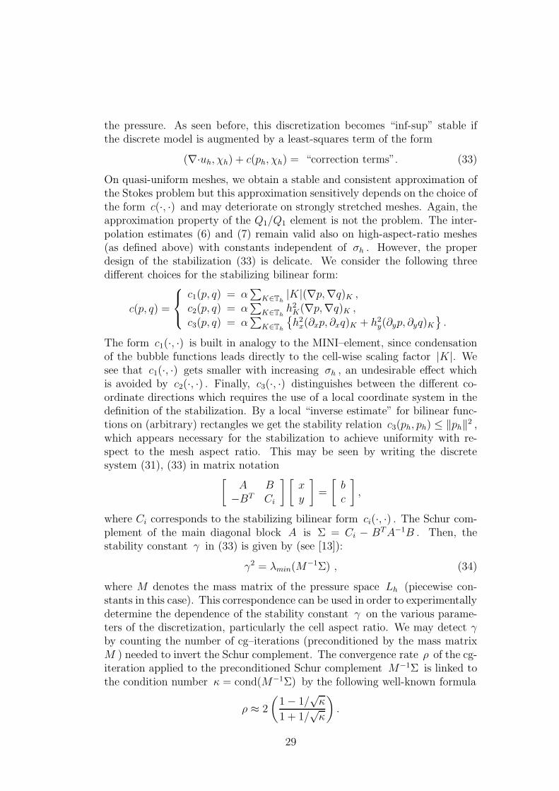
the pressure. As seen before, this discretization becomes “inf-sup” stable ifthe discrete model is augmented by a least-squares term of the form

(∇·uh, χh) + c(ph, χh) = “correction terms”. (33)

On quasi-uniform meshes, we obtain a stable and consistent approximation ofthe Stokes problem but this approximation sensitively depends on the choice ofthe form c(·, ·) and may deteriorate on strongly stretched meshes. Again, theapproximation property of the Q1/Q1 element is not the problem. The inter-polation estimates (6) and (7) remain valid also on high-aspect-ratio meshes(as defined above) with constants independent of σh . However, the properdesign of the stabilization (33) is delicate. We consider the following threedifferent choices for the stabilizing bilinear form:

c(p, q) =

c1(p, q) = α∑

K∈Th|K|(∇p,∇q)K ,

c2(p, q) = α∑

K∈Thh2K(∇p,∇q)K ,

c3(p, q) = α∑

K∈Th

h2x(∂xp, ∂xq)K + h2

y(∂yp, ∂yq)K.

The form c1(·, ·) is built in analogy to the MINI–element, since condensationof the bubble functions leads directly to the cell-wise scaling factor |K|. Wesee that c1(·, ·) gets smaller with increasing σh , an undesirable effect whichis avoided by c2(·, ·) . Finally, c3(·, ·) distinguishes between the different co-ordinate directions which requires the use of a local coordinate system in thedefinition of the stabilization. By a local “inverse estimate” for bilinear func-tions on (arbitrary) rectangles we get the stability relation c3(ph, ph) ≤ ‖ph‖2 ,which appears necessary for the stabilization to achieve uniformity with re-spect to the mesh aspect ratio. This may be seen by writing the discretesystem (31), (33) in matrix notation

[A B

−BT Ci

] [xy

]=

[bc

],

where Ci corresponds to the stabilizing bilinear form ci(·, ·) . The Schur com-plement of the main diagonal block A is Σ = Ci − BTA−1B . Then, thestability constant γ in (33) is given by (see [13]):

γ2 = λmin(M−1Σ) , (34)

where M denotes the mass matrix of the pressure space Lh (piecewise con-stants in this case). This correspondence can be used in order to experimentallydetermine the dependence of the stability constant γ on the various parame-ters of the discretization, particularly the cell aspect ratio. We may detect γby counting the number of cg–iterations (preconditioned by the mass matrixM ) needed to invert the Schur complement. The convergence rate ρ of the cg-iteration applied to the preconditioned Schur complement M−1Σ is linked tothe condition number κ = cond(M−1Σ) by the following well-known formula

ρ ≈ 2

(1 − 1/

√κ

1 + 1/√κ

).

29

These test calculations use a sequence of anisotropic grids obtained by one-directional refinements. The results are given in Table 1.

Table 1: Number of cg–iterations; from Becker [7].

σ 2 4 8 16 32 64 128

c1 8 18 39 98 559 ∗ ∗c2 8 18 39 88 193 ∗ ∗c3 8 16 29 31 29 27 24

Figure 17: Pressure isolines for a jet flow in a channel calculation with the Q1/Q1

element using isotropic stabilization (top and middle) compared to the anisotropicstabilization (bottom); from Becker [7].

The interpretation of these observations is as follows: The increase of thestability constant for c1(·, ·) stems from the fact, that γ ≈ σ−2 → 0 withincreasing aspect ratio, whereas the bad behavior of c2(·, ·) can be explained bythe growth of λmax(Σ) ≈ σ2 due to fact that we only have c2(p, q) ≤ σ‖p‖‖q‖ .We also see that the anisotropic stabilization by c3(·, ·) leads to an aspect-ratio-independent behavior. Similar effects are also observed for the accuracyof the different stabilizations; see Becker [7] and [13].

Open Problem 3.1: Prove the approximation property (27) on general mesh-es with arbitrary aspect ratio σh. The special case of tensor-product mesheshas been treated in Becker [7] (see also Apel [3].

30

3.5 Treatment of dominant transport

In the case of higher Reynolds numbers (e.g., Re > 1000 for the 2-D driven cav-ity, and Re > 100 for the flow around an cylinder) the finite element models(19), (20) or (19), (25) may become unstable since they essentially use central-differences-like discretization of the advective term. This “instability” mostfrequently occurs in form of a drastic slow-down or even break-down of theiteration processes for solving the algebraic problems; in the extreme case thepossibly existing “mathematical” solution contains strongly oscillatory com-ponents without any physical meaning. In order to avoid these effects someadditional numerical damping is required. The use of simple first-order artifi-cial viscosity is not advisable since it introduces too much numerical damping.Below, we describe two approaches used in the context of finite element dis-cretization: i) an adaptive upwinding, and ii) the streamline diffusion method.Alternative techniques are the “characteristics Galerkin method” (for nonsta-tionary flows) and the “discontinuous finite element method” which requiremajor changes in the discretization and will therefore not be discussed here;for references see Pironneau [67], Morton [63] and Johnson [51].

3.5.1 Upwinding

In the finite element context “upwinding” can be defined in a quite natu-ral way; see, e.g., Tobiska/Schieweck [90] and Turek [97], and the literaturecited therein. Here, the upwinding effect is accomplished in the evaluatingof the advection term through shifting integration points into the upwind di-rection. This modification leads to system matrices which have certain M-matrix properties and are therefore amenable to efficient and robust solutiontechniques. This is widely exploited in the finite element codes described inSchreiber/Turek [83], Turek [97] and Schieweck [82].

Following [97], we briefly describe the upwind strategy for the noncon-forming “rotated” bilinear Stokes element. Each quadrilateral K ∈ Th isdivided into eight barycentric fragments Sij, and for each edge Γl and midpoint ml on Γl the “lumping region” Rl is defined by Rl := ∪k∈Λl

Slk , whereΛl = k,ml and mk belong to the same element K. The boundary of thelumping region Rl consists of the edges Γlk := ∂Slk∩∂Skl, i.e., ∂Rl = ∪k∈Λl

Γlk.In this way we obtain an edge oriented partition of the mesh domain Ωh = ∪lRl.

@@

@@

@@

@@

s

s

s smk mm

ml

mn

Slk Slm

Skl Sml

Skn Smn

Snk Snm

@

@@

@@

@@

@

@@

@@

@@

@@s

s

@@

@@

@@

@@

mk

mlRl

K K ′

31

A modification of the nonlinear form n(uh, vh, wh) is now defined by

nh(uh, vh, wh) :=∑

K,l

(1 − λlk(uh)) (vh(mk) − vh(ml))wh(ml)

∫

Γl

uh·nlk ds ,

where λlk are parameters depending on the local flux direction. Setting

x :=1

ν

∫

Γlk

uh·nlk ds ,

possible choices are

λlk :=

1, for x ≥ 00, for x < 0

(“simple upwinding”),

λlk :=

(1/2 + x)/(1 + x), for x ≥ 01/(2 − 2x), for x < 0

(“Samarskij upwinding”),

It can be be shown (see Tobiska/Schieweck [90]) that this upwind scheme is offirst order accurate and, what is most important, the main diagonal blocks ofthe corresponding system matrix A + N(·) become M-matrices. This is thekey property for its inversion by fast multigrid algorithms.

The described upwind discretization can generically be extended to thethree dimensional case. An analogous construction is possible for the con-forming Q1/Q1 element with pressure stabilization also in two as well as inthree dimensions; see Harig [38].

3.5.2 Streamline diffusion

The idea of “streamline diffusion” is to introduce artificial diffusion acting onlyin the transport direction while maintaining the second-order consistency ofthe scheme. This can be achieved in various ways, by augmenting the testspace by direction-oriented terms resulting in a “Petrov-Galerkin method”, orby adding certain least-squares terms to the discretization. For the (stationary)Navier-Stokes problem, we propose the following variant written in terms ofpairs φ, χ ∈ H×L : Find vh ∈ vinh + Hh and ph ∈ Lh , such that

ah(vh, φh) + nh(vh, vh, φh) + bh(ph,∇·φh) + sh(vh, ph, φh, χh)= (f, φh) + rh(vh, ph, φh, χh) (35)

for all φh, χh ∈ H×Lh , where, with some “reference velocity” vh ,

sh(vh, ph, φh, χh) =∑

K∈Th

δK

(∇ph + vh·∇vh,∇χh + vh·∇φh)K

+(∇·vh,∇·φh)K,

rh(vh, ph, φh, χh) =∑

K∈Th

δK(f + ν∆vh,∇χh + vh·∇φh)K .

32

The stabilization parameters δK are chosen according to

δK = minh2

K

ν,hK|v|K

. (36)

This discretization contains several features. The first term in the sum

∑

K∈Th

δK(∇ph,∇χh)K + (vh·∇vh, vh·∇φh)K + (∇·vh,∇·φh)K

stabilizes the pressure-velocity coupling for the conforming Q1/Q1 Stokes el-ement, the second term stabilizes the transport operator, and the third termenhances mass conservation. The other terms introduced in the stabilizationare correction terms which guarantee second-order accuracy for the stabilizedscheme. Theoretical analysis shows that this kind of Galerkin stabilization ac-tually leads to an improvement over the standard upwinding scheme, namelyan error behavior like O(h3/2) for the finite elements described above; see To-biska/Verfurth [91], and also Braack [17] where the same kind of stabilizationhas been applied for weakly compressible flows with chemical reactions. Forlinear convection-diffusion problems the streamline diffusion method is knownto have even O(h2) convergence on fairly general meshes; see [107].

Open Problem 3.2: Derive a strategy for choosing the stabilization parameterδK in the streamline diffusion method on general meshes with arbitrarily largeaspect ratio σh .

Open Problem 3.3: The streamline diffusion method (like the least-squarespressure stabilization) leads to a scheme which lacks local mass conservation.Recently, for convection-diffusion problems an alternative approach has beenproposed which uses a “discontinuous” Galerkin approximation on the trans-port term and combines (higher-order) upwinding features with local mass con-servation. The extension of this method to the incompressible Navier-Stokesequations (and its practical realization) has yet to be done.

33

4 Time discretization and linearization

We now consider the nonstationary Navier-Stokes problem: Find v ∈ vin +Hand p ∈ L , such that v(0) = v0 and

(∂tv, ϕ) + a(v, ϕ) + n(v, v, ϕ) + b(p, φ) = (f, ϕ) , ∀ ϕ ∈ H , (1)

b(χ, v) = 0 , ∀ χ ∈ L . (2)

The choice of the function spaces H ⊂ H1(Ω)d and L ⊂ L2(Ω) depends againon the specific boundary conditions chosen for the problem to be solved; seethe discussion in Section 2.

In the past, explicit time stepping schemes have been commonly used innonstationary flow calculations, mainly for simulating the transition to steadystate limits. Because of the severe stability problems inherent to this approach(for moderately sized Reynolds numbers) the very small time steps requiredprohibited the accurate solution of really time dependent flows. In implicittime stepping one distinguishes traditionally between two different approachescalled the “Method of Lines” and the “Rothe Method”.

4.1 The Rothe Method

In the “Rothe Method”, at first, the time variable is discretized by one ofthe common time differencing schemes; for a general account of such schemessee, e.g., Thomee [89]. For example, the backward Euler scheme leads to asequence of Navier-Stokes-type problems of the form:

k−1n (vn−vn−1, φ) + a(vn, φ) + n(vn, vn, φ) + b(pn, φ) = (fn, φ), (3)

b(χ, vn) = 0 . (4)

for all φ, χ ∈ H × L , where kn = tn − tn−1 is the time step. Each of theseproblems is then solved by some spatial discretization method as describedin the preceding section. This provides the flexibility to vary the spatial dis-cretization, i.e. the mesh or the type of trial functions in the finite elementmethod, during the time stepping process. In the classical Rothe method thetime discretization scheme is kept fixed and only the size of the time step maychange. The question of how to deal with varying spatial discretization withina time-stepping process while maintaining higher-order accuracy and conser-vation properties is currently subject of intensive research. It is essential todo the mesh-transfer by L2 projection which is costly, particularly in 3D if fullremeshing is used in each time step, but is easily manageable if only meshesfrom a family of hierarchically ordered meshes are used.

4.2 The Method of Lines

The traditional approach to solving time-dependent problems is the “Methodof Lines”. At first, the spatial variable is discretized, e.g. by a finite element

34

method as described in the preceding section leading to a system of ordinarydifferential equations of the form:

Mx(t) + Ax(t) +N(x(t))x(t) +By(t) = b(t) , (5)

−BTx(t) + Cy(t) = c(t), t > 0 , (6)

with the initial value x(0) = x0 . The mass matrix M , the stiffness matrixA and the gradient matrix B are as defined above in Section 3. The matrixC and the right-hand side c stem from the pressure stabilization when usingthe conforming Q1/Q1 Stokes element. Further, the (nonlinear) matrix N(·)is thought to contain also all terms arising through the transport stabilizationby upwinding or streamline diffusion. For abbreviation, we will sometimes usethe notation A(·) := A+N(·) .

For solving this ODE system, one now applies a time differencing scheme.The most frequently used schemes are the so–called “One-Step-θ Schemes”:

One-step θ-scheme: Step tn−1 → tn (k = time step):

[M + θkAn]xn +Byn = [M − (1−θ)kAn−1]xn−1 + θkbn + (1−θ)kbn−1

−BTxn + Cyn = cn ,

where xn ≈ x(tn) and An := A(xn) . Special cases are the “forward Eulerscheme” for θ = 0 (first-order explicit), the backward Euler scheme for θ = 1(first-order implicit, strongly A-stable), and the most popular Crank-Nicolsonscheme for θ = 1/2 (second-order implicit, A-stable). These properties canbe seen by applying the method to the scalar model equation x = λx . In thiscontext it is related to a rational approximation of the exponential function ofthe form

Rθ(−λ) =1 − (θ − 1

2)λ

1 + θλ= e−λ + O

((θ − 1

2)|λ|2 + |λ|3

), |λ| ≤ 1 .

The most robust implicit Euler scheme ( θ = 1 ) is very dissipative and there-fore not suitable for computing really nonstationary flow. In contrast, theCrank-Nicolson scheme has only very little dissipation but occasionally suffersfrom unexpected instabilities caused by the possible occurrence of rough per-turbations in the data which are not damped out due to the only weak stabilityproperties of this scheme (not strongly A-stable). This defect can in principlebe cured by an adaptive step size selection but this may enforce the use of anunreasonably small time step, thereby increasing the computational costs. Fora detailed discussion of this issue see [71]. A good time-stepping scheme of thedescribed type should possess the following properties:

• A-stability (⇒ local convergence): |R(−λ)| ≤ 1

• Global stability (⇒ global convergence):

limReλ→∞|R(−λ)| ≤ 1 −O(k) .

35

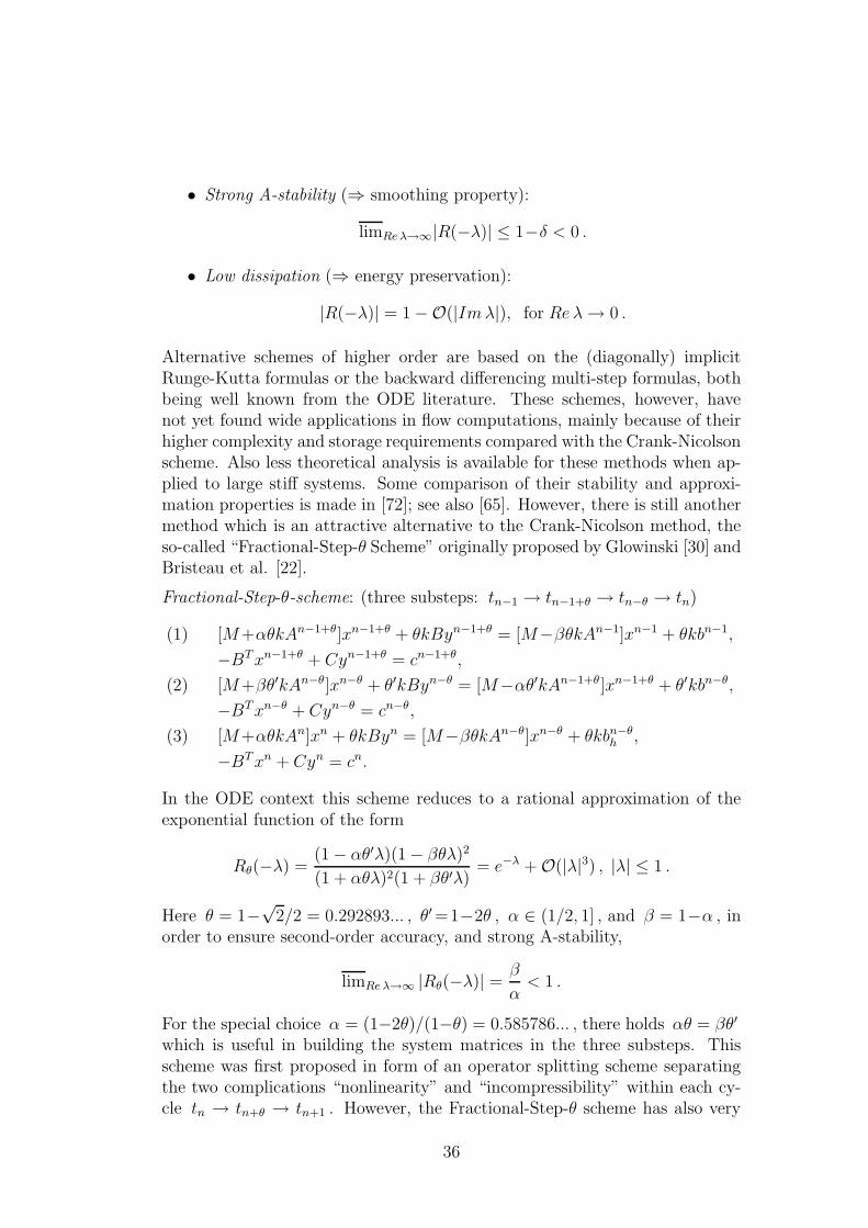
• Strong A-stability (⇒ smoothing property):

limReλ→∞|R(−λ)| ≤ 1−δ < 0 .

• Low dissipation (⇒ energy preservation):

|R(−λ)| = 1 −O(|Imλ|), for Reλ→ 0 .

Alternative schemes of higher order are based on the (diagonally) implicitRunge-Kutta formulas or the backward differencing multi-step formulas, bothbeing well known from the ODE literature. These schemes, however, havenot yet found wide applications in flow computations, mainly because of theirhigher complexity and storage requirements compared with the Crank-Nicolsonscheme. Also less theoretical analysis is available for these methods when ap-plied to large stiff systems. Some comparison of their stability and approxi-mation properties is made in [72]; see also [65]. However, there is still anothermethod which is an attractive alternative to the Crank-Nicolson method, theso-called “Fractional-Step-θ Scheme” originally proposed by Glowinski [30] andBristeau et al. [22].

Fractional-Step-θ-scheme: (three substeps: tn−1 → tn−1+θ → tn−θ → tn)

(1) [M+αθkAn−1+θ]xn−1+θ + θkByn−1+θ = [M−βθkAn−1]xn−1 + θkbn−1,

−BTxn−1+θ + Cyn−1+θ = cn−1+θ,

(2) [M+βθ′kAn−θ]xn−θ + θ′kByn−θ = [M−αθ′kAn−1+θ]xn−1+θ + θ′kbn−θ,

−BTxn−θ + Cyn−θ = cn−θ,

(3) [M+αθkAn]xn + θkByn = [M−βθkAn−θ]xn−θ + θkbn−θh ,

−BTxn + Cyn = cn.

In the ODE context this scheme reduces to a rational approximation of theexponential function of the form

Rθ(−λ) =(1 − αθ′λ)(1 − βθλ)2

(1 + αθλ)2(1 + βθ′λ)= e−λ + O(|λ|3) , |λ| ≤ 1 .

Here θ = 1−√

2/2 = 0.292893... , θ′ =1−2θ , α ∈ (1/2, 1] , and β = 1−α , inorder to ensure second-order accuracy, and strong A-stability,

limReλ→∞ |Rθ(−λ)| =β

α< 1 .

For the special choice α = (1−2θ)/(1−θ) = 0.585786... , there holds αθ = βθ′

which is useful in building the system matrices in the three substeps. Thisscheme was first proposed in form of an operator splitting scheme separatingthe two complications “nonlinearity” and “incompressibility” within each cy-cle tn → tn+θ → tn+1 . However, the Fractional-Step-θ scheme has also very

36

attractive features as a pure time-stepping method. It is strongly A-stable, forany choice of α ∈ (1/2, 1] , and therefore possesses the full smoothing propertyin the case of rough initial data, in contrast to the Crank–Nicolson scheme (caseα = 1/2). Furthermore, its amplification factor has modulus |R(−λ)| ≈ 1 ,for λ approaching the imaginary axis (e.g., |R(−0.8i)| = 0.9998... ), which isdesirable in computing oscillatory solutions without damping out the ampli-tude. Finally, it also possesses very good approximation properties, i.e., onecycle of length (2θ+θ′)k = k provides the same accuracy as three steps of theCrank-Nicolson scheme with total step length k/3 ; for more details on thiscomparison see [72] and [65].

We mention some theoretical results on the convergence of these schemes.For the Crank-Nicolson Scheme combined with spatial discretization as de-scribed in Section 3, an optimal-order convergence estimate

‖vnh − v(·, tn)‖ = O(h2 + k2) (7)

has been given in [44]. This estimate requires some additional stabilizationof the scheme but then holds under realistic assumptions on the data of theproblem. A similar result has been shown by Muller [64] for the Fractional-Step θ-Scheme. Due to its stronger damping properties (strong A-stability)this scheme does not require extra stabilization.

4.2.1 Computational tests

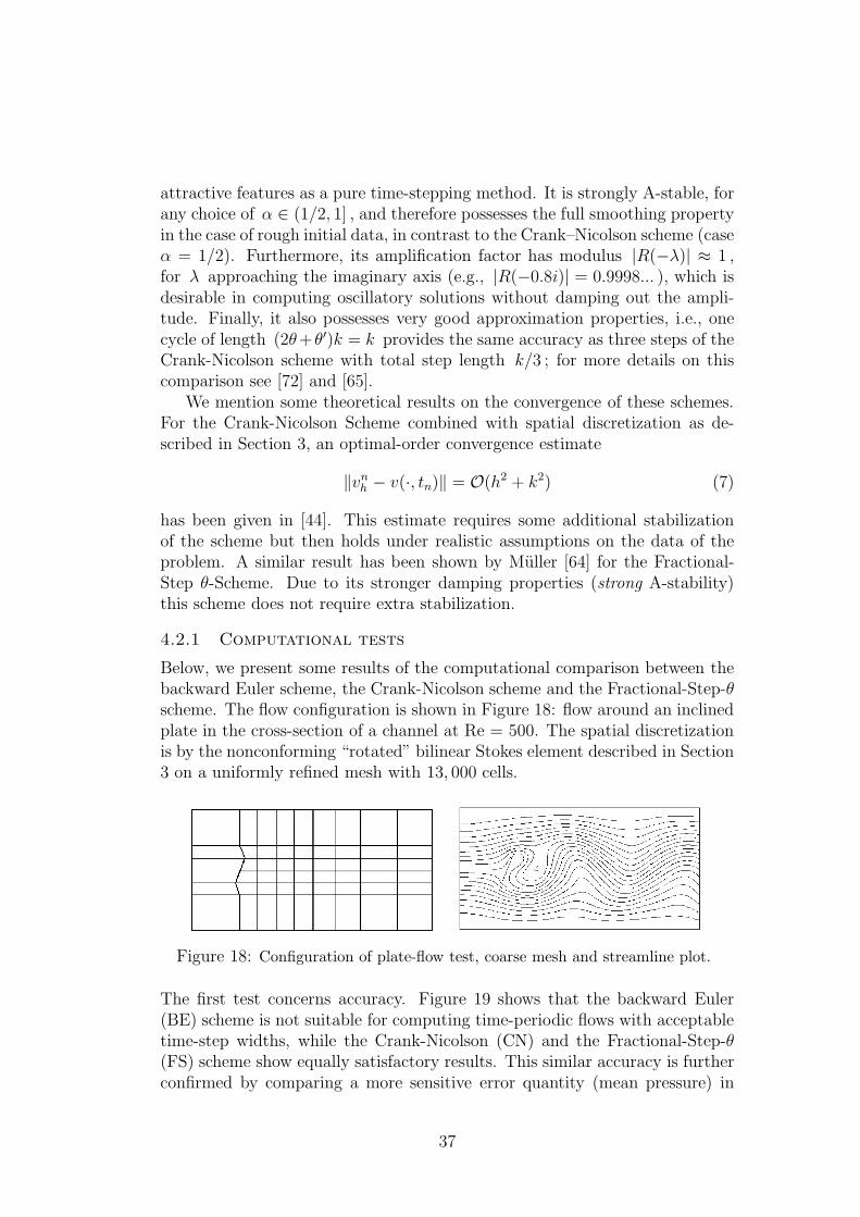
Below, we present some results of the computational comparison between thebackward Euler scheme, the Crank-Nicolson scheme and the Fractional-Step-θscheme. The flow configuration is shown in Figure 18: flow around an inclinedplate in the cross-section of a channel at Re = 500. The spatial discretizationis by the nonconforming “rotated” bilinear Stokes element described in Section3 on a uniformly refined mesh with 13, 000 cells.

Figure 18: Configuration of plate-flow test, coarse mesh and streamline plot.

The first test concerns accuracy. Figure 19 shows that the backward Euler(BE) scheme is not suitable for computing time-periodic flows with acceptabletime-step widths, while the Crank-Nicolson (CN) and the Fractional-Step-θ(FS) scheme show equally satisfactory results. This similar accuracy is furtherconfirmed by comparing a more sensitive error quantity (mean pressure) in

37

Figure 20. Finally, we look at the stability of the schemes. Figure 21 demon-strates the lack of robustness of the Crank-Nicolson scheme combined withlinear time-extrapolation in the nonlinearity for larger time steps.

Figure 19: Pressure isolines of the plate-flow test: BE scheme with 3k = 1 (topleft), BE scheme with 3k = 0.1 (top right), CN scheme with 3k = 1 (bottom left),FS scheme with k = 1 (bottom right); from [65].

10 20 30 40 50 60 10 20 30 40 50 60

Figure 20: Mean pressure plots for the plate test with fully implicit treatment ofthe nonlinearity; left: CN scheme with 3k = 0.33; right: FS scheme with k = 0.33,both compared to a reference solution (dotted line); from[65].

10 20 30 40 50 60 10 20 30 40 50 60

Figure 21: Mean pressure plots for the plate test with linear time-extrapolation;left: CN scheme with 3k = 0.11; right: FS scheme with k = 0.11, both compared toa reference solution (dotted line); [65].

38

4.3 Splitting and projection schemes

As already mentioned, the Fractional-Step-θ scheme was originally introducedas an operator splitting scheme in order to separate the two main difficultiesin solving problem (1) namely the nonlinearity causing nonsymmetry and theincompressibility constraint causing indefiniteness. At that time, handlingboth complications simultaneously was not feasible. Therefore, the use ofoperator splitting seemed the only way to compute nonstationary flows. Usingthe notation from above, the splitting scheme reads as follows (suppressinghere the terms stemming from pressure stabilization).

Splitting-Fractional-Step-θ Scheme:

(1) [M + αθkA]xn−1+θ + θkByn−1+θ = [M − βθkA]xn−1 + θkbn−1 −−θkNn−1xn−1,

BTxn−1+θ = 0 ,

(2) [M + βθ′kAn−θ]xn−θ = [M − αθ′kAn−1+θ]xn−1+θ − θ′kByn−θ + θ′kbn−θ,

.....

(3) [M + αθkA]xn + θkByn = [M − βθkA]xn−θ − θkNn−θxn−θ + θkbn−θ,

BTxn = 0 .

The first and last step solve linear Stokes problems treating the nonlinearityexplicitly, while in the middle step a nonlinear Burgers-type problem (withoutincompressibility constraint) is solved. The symmetric form of this schemefollows the ideas from Strang [87], in order to achieve a second-order splittingapproximation. The results of Muller [64] suggest that the optimal-order con-vergence estimate (7) remains true also for this splitting scheme. However, acomplete proof under realistic assumptions is still missing.

Open Problem 4.1: Prove that the Splitting-Fractional-Step-θ scheme isactually second order accurate for all choices of the parameter α ∈ (1

2, 1] .

In these days, the efficient solution of the nonlinear incompressible Navier-Stokes equations is standard by the use of new multigrid techniques. Hence,the splitting of nonlinearity and incompressibility is no longer an importantissue. One of these new approaches uses the Fractional-Step-θ scheme in com-bination with the idea of a “projection method” due to Chorin [24]; for asurvey see Gresho/Sani [35]. Finally, Turek [95] (see also [97]) has designedthe “Discrete Projection Fractional-Step-θ scheme” as component in his solverfor the nonstationary Navier-Stokes problem.

Next, we address the problem of how to deal with the incompressibilityconstraint ∇·v = 0 . The traditional approach is to decouple the continuityequation from the momentum equation through an iterative process (again“operator splitting”). There are various schemes of this kind in the litera-ture referred to, e.g., as “quasi-compressibility method”, “projection method”,“SIMPLE method”, etc. All these methods are based on the same principle

39

idea. The continuity equation ∇·v = 0 is supplemented by certain stabilizingterms involving the pressure, e.g.,

∇·v + εp = 0, (8)

∇·v − ε∆p = 0, ∂np|∂Ω = 0, (9)

∇·v + ε∂tp = 0, p|t=0 = 0, (10)

∇·v − ε∂t∆p = 0, ∂np|∂Ω = 0, p|t=0 = 0, (11)

where the small parameter ε is usually taken as ε ≈ hα , or ε ≈ kβ , dependingon the purpose of the procedure. For example, (8) corresponds to the classical“penalty method”, and (9) is the simplest form of the “least squares pres-sure stabilization” scheme (11) described above, with ε ≈ h2 in both cases.Further, (10) corresponds to the “quasi-compressibility method”.

These approaches are closely related to the classical “projection method” ofChorin [24]. Since this method used to be particularly attractive for computingnonstationary incompressible flow, we will discuss it in a some detail. Forsimplicity consider the case of homogeneous Dirichlet boundary conditions,v|∂Ω = 0 . The projection method reads as follows. For an admissible initialvalue v0 , choose a time step k , and solve for n ≥ 1 :

(i) vn ∈ H (implicit “Burgers step”):

k−1(vn − vn−1) − ν∆vn + vn·∇vn = fn. (12)

(ii) vn = P vn ∈ J0(Ω) (“Projection step”):

∇·vn = 0, n·vn|∂Ω = 0. (13)

Here, the function space J0(Ω) is obtained through the completion of thespace φ ∈ D(Ω),∇·φ ≡ 0 of solenoidal test functions with respect to thenorm of L2(Ω) . This time stepping scheme can be combined with any spatialdiscretization method, e.g. the finite element methods described in Section 3.The projection step (ii) can equivalently be expressed in the form

(ii’) vn = vn + k∇pn, (14)

with some “pressure” pn ∈ H1(Ω) , which is determined by the properties

(ii”) ∆pn = k−1∇·vn, ∂npn|∂Ω = 0. (15)

This amounts to a Poisson equation for pn with zero Neumann boundaryconditions. It is this non-physical boundary condition, ∂np

n|∂Ω = 0 , which

has caused a lot of controversial discussion about the value of the projectionmethod. Nevertheless, the method has proven to work well for representing thevelocity field in many flow problems of physical interest (see, e.g. Gresho [32]and Gresho/Chan [33]). It is very economical as it requires in each time step

40

only the solution of a (nonlinear) advection-diffusion system for vn (of Burgersequation type) and a scalar Neumann problem for pn . Still, it was argued thatthe pressure pn were a mere fictitious quantity without any physical relevance.It remained the question: How can such a method work at all? A challengingproblem for mathematical analysis!

The first convergence results for the projection method was already givenby Chorin, but concerned only cases with absent rigid boundaries (all-spaceor spatially periodic problems). Later on, qualitative convergence was showneven for the pressure, but in a measure theoretical sense, too weak for practicalpurposes. Only recently, stronger results on the error behavior of this methodhave been obtained (see, e.g., Shen [84, 85] as well as [73], and the literaturecited therein). The best known error estimate is

‖vn − v(tn)‖Ω + ‖pn − p(tn)‖Ω′ = O(k), (16)

where Ω′ ⊂⊂ Ω is a subdomain with positive distance to the boundary ∂Ω .This shows that the quantities pn are indeed reasonable approximations tothe pressure p(tn) , and finally confirms that Chorin’s original method is afirst-order time stepping scheme for the incompressible Navier-Stokes problem.The key to this result is the re-interpretation of the projection method in thecontext of the “pressure stabilization methods”. To this end, one inserts thequantity vn−1 = vn−1−k∇pn−1 into the momentum equation, obtaining

k−1(vn − vn−1) − ν∆vn + (vn·∇)vn + ∇pn−1 = fn, vn|∂Ω = 0, (17)

∇·vn − k∆pn = 0, ∂npn|∂Ω = 0. (18)

This looks like an approximation of the Navier-Stokes equations involving afirst-order (in time) “pressure stabilization” term, i.e., the projection methodcan be viewed as a pressure stabilization method with a global stabilizationparameter ε = k , and an explicit treatment of the pressure term. Moreover, itappears that the pressure error is actually confined to a small boundary stripof width δ ≈

√νk and decays exponentially into the interior of Ω . In fact, it

was conjectured that, setting d(x) = dist(x, ∂Ω) ,

|pn(x) − p(x, tn)| ≤ c exp

(−αd(x)√

νk

)√k +O(k). (19)

This conjecture is supported by numerical experiments for the pressure stabi-lization method applied to the stationary Stokes problem and by some modelsituation analysis in E/Liu [25]. The analysis of this boundary layer phe-nomenon requires the study of the singularly perturbed Neumann problem

(ν−1∇·∆−1

D ∇− ǫ∆N

)q = ǫ∆p, in Ω, ∂nq|∂Ω = ∂np|∂Ω, (20)

where ∆D denotes the Laplacian operator corresponding to Dirichlet bound-ary conditions. Clearly, ∇·∆−1

D ∇ is a zero-order operator mapping L2(Ω)

41

into L2(Ω) . For this problem, one would like to know a decay estimate of theform

‖q‖Ωδ≤ c exp

(−α δ√

ǫ

)‖∇p‖ + cνǫ ‖∆p‖, (21)

for interior subdomains Ωδ := x ∈ Ω, dist(x, ∂Ω) > δ , from which a point-wise result like (19) could be inferred. Such an estimate could be proven in[73] only for the case that the “global” operator ∇·∆−1

D ∇ is replaced by the“local” identity operator. In the general case the corresponding result is stillan open problem.

Open Problem 4.2: Prove an analogue of the a priori decay estimate (21)for the non-local operator ∇·∆−1

D ∇ .

The occurrence of the pressure boundary layer is demonstrated in Figure 22for a simple model problem on the unit square with known polynomial solution.It is even possible to recover the optimal-order accuracy of the pressure, O(h2) ,at the boundary by postprocessing, e.g. by linear or quadratic extrapolationof pressure values from the interior of the domain; see Figure 23 and Blum [15]for more details on this matter.

Figure 22: Sequence of pressure-error isolines obtained by the Chorin scheme withk = 2.5·10−2, 6.25·10−3, 1.56·10−3 (model problem with ν = 1 on the square); fromProhl [69].

Figure 23: Pressure error plots for a polynomial Stokes solution before (left) andafter (right) correction by extrapolation to the boundary; from Blum [15].

42

An important step towards the solution of the “boundary layer problem”has been made in Prohl [69, 70] by introducing the “Chorin-Uzawa scheme”,which reads as follows:

(i) Implicit “Burgers step”:

k−1(vn − vn−1) − ∆vn + vn·∇vn + ∇(pn−1 − pn−1) = fn, vn|∂Ω = 0.

(ii) Pressure Poisson problem:

∆pn = k−1∇·vn, ∂npn|∂Ω = 0.

(iii) Pressure and velocity update:

vn = vn − k∇pn, pn = pn−1 − α∇·vn, α < 1.

The reference to the name “Uzawa” is due to the fact that this scheme par-tially resembles the structure of the well-known Uzawa algorithm for solvingstationary saddle-point problems; see Girault/Raviart [29]. It corresponds toa quasi-compressibility method using the regularization

∇·vn + α−1k∂tpn = 0. (22)

This splitting scheme does not introduce a singular perturbation in the pres-sure equation and is therefore supposed to be free of any spatial boundarylayer. However, it suffers from a “boundary layer” at time t = 0 in case ofnatural initial data not satisfying unrealistic global compatibility conditions;recall Section 2 for a discussion of such conditions. The conjectured suppres-sion of the spatial pressure boundary layer by the Chorin-Uzawa scheme isconfirmed by computational tests; see the example presented in Figure 24.A supporting analysis has been given in Prohl [70] for a modification of theChorin-Uzawa method to a “multi-component scheme” which allows for theconvergence estimate

‖pn − p(tn)‖ ≤ ck, tn ≥ 1. (23)

Figures 24 show pressure error plots obtained for a given polynomial solutionon the unit-square with viscosity ν = 1 ; the time step is k = 1/100 and thespatial discretization uses theQ1/Q1 Stokes element with pressure stabilizationon a uniform mesh with mesh-size h = 1/64 .

Figure 24: Pressure error plots for a polynomial solution produced by the standardChorin scheme (left) and the Chorin-Uzawa scheme (right); from Prohl [69, 70].

43

The projection approach can be extended to formally higher order projec-tion methods. The most popular example is Van Kan’s Method [100]: Foradmissible starting values v0 and p0 compute, for n ≥ 1 and some α ≥ 1

2:

(i) vn ∈ H (second order implicit Burgers step), satisfying

k−1(vn − vn−1) − 12ν∆(vn + vn−1) + vn·∇vn + ∇pn−1 = fn−1/2;

(ii) pn ∈ H1(Ω) : vn = vn − αk∇(pn − pn−1) .

A careful examination of this scheme shows that it can also be interpreted asa certain pressure stabilization method using a stabilization of the form

∇·v − αk2∂t∆p = 0, in Ω, ∂np|∂Ω = 0, (24)

i.e., this method may be viewed as an (implicit) quasi-compressibility methodof the form (11) with ε ≈ k2 ; see [74] and Shen [86].

The projection method may be combined with any of the spatial discretiza-tions described in Section 3. It should be remarked that the simple first-orderChorin scheme is not suitable for computing stationary limits since it hasnot the from of a fixed-point iteration. In contrast to that, the second-orderscheme of Van Kan is designed as a defect-correction iteration and may there-fore lead to convergence towards steady state solutions. However, in this caseit requires extra pressure stabilization when used together with the conform-ing Q1/Q1 Stokes element; in fact the stabilizing effect of the projection stepdisappears as αk2∂t∆p→ 0 .

Open Problem 4.3: The efficient use of projection methods requires an au-tomatic time-step-size control which should monitor deviation from the fullycoupled solution. Design such a method for high-order schemes.

44

5 Solution of the algebraic systems

In this section, we describe solution algorithms for the finite-dimensional prob-lems arising from the discretization presented in the previous sections. Theseproblems form huge and highly nonlinear algebraic systems with a character-istic structure which is exploited by the algorithms. The solution procedureconsists of several nested loops. Usually the outermost loop is an implicittime-iteration. In each time step, the arising nonlinear system is solved by aquasi-Newton or defect-correction iteration. The discretization by finite ele-ments leads to a sparse structure in the system matrices which is exploited bythe iterative solution method. Even in the case of the Laplace operator (whichis always a part of the system), the inversion by a direct solver or a simpleiterative scheme like the “conjugate gradient” (CG) method is prohibitive dueto the bad conditioning of the matrix with decreasing mesh size. Therefore,the use of multigrid methods is mandatory, either directly as solvers or aspreconditioners for a robust iterative schemes like the “generalized minimalresidual” (GMRES) algorithm. Since the systems to be solved are in generalnon-symmetric and indefinite, the construction of “good” multigrid algorithmsrequires special care.

5.1 Linearization

The time stepping schemes described above require in each time step the so-lution of nonlinear systems of the form

[σM + νA +N(v)]v +Bp = g , (1)

−BT v + ǫCp = c , (2)

where σ = (θk)−1 and (on a quasi-uniform mesh) ǫ ∼ h2 . The operatorsinvolved correspond to differential operators as follows:

M ∼ id., A ∼ −diag(∆D), N(v) ∼ v·∇,B ∼ ∇, −BT ∼ ÷, C ∼ −∆N ,

where ∆D and ∆N denote the Laplacian operator combined with (homoge-neous) Dirichlet or Neumann boundary conditions, respectively. The right-hand sides g and c contain information from the preceding time level. Hereand below, the same notation is used for the (discrete) velocity v and pressurep and the corresponding nodal vectors. The following iteration schemes areformulated on the continuous level without incorporating stabilization, i.e., weset ǫ = 0 and c = 0 .

a) Newton method:Starting from some initial values v0, p0 ∈ H×L (for example, taken from thepreceding time level), one iterates:

1. Defect: dl = g −(σM + νA+N(vl)

)vl − Bpl.

45

2. Correction: [σM + νA+N ′(vl)]wl +Bql = dl, BTwl = 0.

3. Update: vl+1 = vl + λlwl, pl+1 = pl + λlq

l (λl damping factor).

This iteration has been observed to converge very fast, provided that it con-verges at all. The problem is its lack of robustness particularly in the case oflarger Reynolds numbers. This is due to the structure of the operator to beinverted in each iteration step:

N ′(v)w = v·∇w + w·∇v.

It contains a reaction term w·∇v which effects the main diagonal of the systemmatrix in an uncontrolled manner and may cause divergence of the iteration.This problem may be avoided by simply dropping the reaction term in theJacobian which results in the following fixed-point defect correction iteration.

b) Fixed-point defect correction:Starting from some initial values v0, p0 ∈ H × L (taken again from the pre-ceding time level), one iterates:

1. Defect: dl = g −(σM + νA+N(vl)

)vl − Bpl.

2. Correction: [σM + νA+N(vl)]wl +Bql = dl, BTwl = 0.

3. Update: vl+1 = vl + λlwl, pl+1 = pl + λlq

l (λl damping factor).

In this scheme the preconditioning operator A′(vl) = vl·∇ only containsa transport term which can be stabilized by any of the methods describedabove: upwinding, streamline diffusion, etc. Normally, within the time step-ping scheme, only a few (usually 3-5) steps of the defect correction iterationare necessary for reducing the initial residual down to the level of the dis-cretization error. This is our method of choice used in the codes mentioned inthe Introduction.

c) Nonlinear multigrid iteration:The multigrid method can be applied directly to the nonlinear system; seeHackbusch [36]. This may lead to faster convergence but its optimization isdifficult and depends very much on the particular problem. Because of thislack of robustness, we do not advocate “nonlinear” multigrid for solving theNavier-Stokes equations.

d) Nonlinear least-squares cg method:The (nonlinear) least squares cg-method for solving systems like (1) has beenproposed by Glowinski/Periaux [31]. Starting from an initial guess x0, a se-quence of approximate solutions (xl)l≥0 is obtained by minimizing the leastsquares functional

‖∇w‖2 → min! (3)

46

where w is determined by v, p through the equation

[σM + νA]w − Bq = “defect” of v, p, BTw = 0. (4)

It can be seen that each nonlinear cg-step actually requires only the solution ofthree linear Stokes problems which can be efficiently done by linear multigridtechniques. This method is very robust as it is based on the minimization ofa positive functional, but the speed of convergence drastically slows down forlarger Reynolds numbers. For example, the 3-D driven cavity problem can besolved by the stationary version of the least squares cg method up to aboutRe = 2000; for further details, see [38].

5.2 Solution of the linearized problems

The problem to be solved has the form[

S B−BT ǫC

] [vp

]=

[gc

], A =

[S B

−BT ǫC

], (5)

where, with some initial guess v ,

S = σM + νA +N(v).

The difficulty with this system is that the matrix A is neither symmetric nordefinite. It is usually too large for the application of direct solvers (like theLU decomposition by Gaussian elimination) and also the traditional iterativemethods (like SOR iteration or Krylov space schemes) do not work sufficientlywell. This suggests the use of multigrid methods which are particularly suitedon very fine meshes. However, the construction of efficient multigrid algorithmsfor solving the indefinite system (5) is not at all straightforward. Therefore,as a simpler alternative the Schur complement approach has become popularwhich will be described in the following subsection.

5.2.1 Schur-complement iteration

In the system matrix A the main block S is regular and usually robust to beinverted. Hence, the velocity unknowns may be eliminated from the systemby inverting S which leads to:

[BTS−1B + ǫC]p = BTS−1g + c , v = S−1(g −Bp). (6)

The “Schur-complement” matrix Σ = BTS−1B + ǫC is regular. Neglectingthe influence of the nonlinear term N(v) , its condition number behaves like

cond(Σ) = O(h−2) for νk ≪ h2, cond(Σ) = O(1) for νk ≫ h2.

This suggests the use of iterative methods for its inversion, e.g., Krylov spacemethods like the GMRES or the bi-cg-stab method. In the essentially non-stationary case, νk ≥ h2 , only a few iteration steps suffice. In nonstationary

47

computations where νk ≪ h2 , preconditioning by an approximation of theNeumann-type operator BTM−1B is necessary. In each iteration step the op-erator S−1 has to be evaluated which amounts to solving a linear transport-diffusion problem. In the case of the nonconforming Q1/P0 Stokes elementscombined with upwind stabilization of advection S becomes an M-matrix.This facilitates the iterative inversion of Σ , particularly by multigrid meth-ods. The non-exact inversion of Σ makes the step q → Σ−1q a preconditioningstep within the iteration for inverting Σ . Hence, the number of inner iterationsteps should be kept fixed during the whole solution process. Another strategyfor compensating for the error in the evaluation of S−1 is to embed the outeriteration (6) into a defect correction process; see Bank, et al., [6]. The conver-gence usually deteriorates for increasing Reynolds number, because of loss of“symmetry”, and for decreasing time step k , because of the bad conditioningof the operator BTB ∼ ∆ . For larger Reynolds number the convergence ofthe Schur complement iteration becomes slow and special preconditioning isnecessary. The construction of effective preconditioners is not easy since theoperator Σ is not available as an explicit matrix. Another stability problemoccurs on meshes containing cells with large aspect ratio. Because of this lackof robustness, the Schur complement method has less potential than the directmultigrid approach which will be described below.

Open Problem 5.1: Derive a formula for the dependence of the conditioningof the Schur complement operator Σ = BTS−1B+ǫC on the Reynolds numberand on the mesh aspect ratio σh .

5.3 Linear multigrid solution

The main idea underlying a multigrid method is the fast reduction of high-frequency error components by “cheap” relaxation (“smoothing”) on the finemeshes and the reduction of the remaining low-frequency error components bydefect correction on coarser meshes (“coarse-grid correction”); see Hackbusch[36] and Wesseling [104], for an introduction to multigrid methods.

5.3.1 Multigrid as a preconditioner

Let A be the finite element system matrix of the linearized equation (5) or anappropriate approximation. While the theory of multigrid is well developedfor scalar elliptic equations, the situation is less clear for complicated systemsas considered in this paper. From mathematical analysis, we know that theuse of the multigrid method as a preconditioner in an outer iteration (e.g., aKrylov space method such as GMRES) requires less restrictive assumptionsthan using the multigrid method directly as a solver. In the first case, de-noting by M the action of a multigrid step, it is sufficient to have an upperbound for the condition of the product MA , whereas in the second case,the eigenvalues of the iteration matrix B = I − MA have to be uniformlybounded away from one. Therefore, we choose the first option to construct

48

a robust iteration scheme for the system (5). As basic solver, one may usethe “generalized minimal residual method” (GMRES) for the preconditionedmatrix MA . Here, the multigrid operator M can be interpreted as a certainapproximate inverse M ≈ A−1 . It is not necessary to calculate this matrixexplicitly; it is sufficient to evaluate the matrix-vector product Mξ , i.e., toapply the multigrid iteration for a fixed right-hand side.

5.3.2 Multigrid as a solver

The multigrid iteration makes use of the hierarchy of finite element spaces

V0 ⊂ V1 ⊂ . . . ⊂ VL ,

obtained, for example, in the course of a systematic mesh refinement process;strategies for an automatic adaptive mesh refinement will be discussed belowin Section 7. The connection between these spaces is given by “prolongationoperators” P l

l−1 : Vl−1 → Vl and “restriction operators” Rl−1l : Vl → Vl−1 . In

the finite element context, these operators are given naturally as

P ll−1 injection, Rl−1

l L2 Projection.

The main ingredients of a multigrid scheme are the smoothing operatorsSl on each grid level 0 ≤ l ≤ L (l=0 corresponding to the coarse initial meshand l = L to the finest mesh). The explicit form of these operators will bedescribed below. The multigrid iteration

Mξ = M(l, z0, ξ), (7)

on level l with initial guess z0 and with m1 pre- and m2 post-smoothingsteps is recursively defined as follows:

Multigrid Algorithm M(l, z0, ξ) for l≥0 :For l= 0, the multigrid algorithm is given by an exact solver M(l, z0, ξ) :=A−1

0 ξ . For l>0 , the following recursive iteration is performed:

1. Pre-smoothing m1 times: z1 := Sm1

l z0.

2. Residual on level l: rl := ξ −Akz1.

3. Restriction to level l−1 : rl−1 := Rlrl.

4. Coarse grid correction starting with q0 = 0: q := M(l−1, q0, rl−1) .

5. Prolongation to level l : z2 := z1 + Pl−1q.

6. Post-smoothing m2 times: M(l, z0, ξ) := Sm2

l z2.

49

If the multigrid recursion is applied γ-times on each mesh-level, one speaksof a V -cycle for γ = 1 and of a W -cycle for γ = 2 . If the multigrid iterationis used only as a preconditioner for a robust outer iteration scheme, usuallythe V -cycle suffices. If multigrid is used as the primary solver, particularly inthe case of nonsymmetric problems, the W -cycle is more robust and thereforeto be preferred. In this case, the F -cycle as indicated in the figure belowis a compromise between V - and W -cycle. The multigrid cycle with γ > 2becomes too expensive and is not used.

4v3v

v2

v1

v0

Figure 25: Scheme of the multigrid V-cycle (left) and the F-cycle (right)

The design of a multigrid algorithm for solving the system (5) requiresspecial care. In particular, the choice of the smoother is a delicate mattersince the standard fixed-point iterations do not work for the indefinite matrixA . This problem can be tackled in various ways.

(1) Damped Jacobi smoother: In the case ǫ > 0 , the matrix A is weakly defi-nite which makes it possible to apply even standard methods like the dampedJacobi iteration. However, the resulting algorithm is not very robust and pa-rameter tuning requires care; see [38] for an application to 3-dimensional modelproblems. For larger Reynolds number the method slows down and multigridconvergence may get lost.

(2) Block-Gauss-Seidel smoother: A simple and successful smoother for thematrix A can be obtained by a cell-wise blocking of the physical variableswithin a global Gauss-Seidel iteration. This was originally proposed by Vanka[101] for a finite difference discretization of the Navier-Stokes problem. Webriefly discuss its analogue for the nonconforming “rotated” Q1/P0 Stokeselement. The velocity and pressure unknowns corresponding to a cell K ora patch of cells are grouped together. Indicating the corresponding elementsystem matrices by index “loc”, these blocks of local velocity and pressureunknowns are simultaneously updated according to

Slocvt+1loc +Blocp

t+1loc = “known”, BT

locvt+1loc = “known”,

where Sloc = σMloc+νAloc+Nloc(vh) . This iteration sweeps over all cell-blocks.The local Stokes problems have the dimension dloc = 9 (in 2D) or dloc = 19(in 3D), respectively. The corresponding matrices (in 2D) are described in thefollowing figure.

50

f×

×

×

×× : node for v© : node for p

Aloc =

Sloc,1 O Bloc,1

O Sloc,2 Bloc,2

−BTloc,1 −BT

loc,2 0

.

For cost reduction, the main diagonal blocks Sloc,i may be “lumped”, Sloc,i ≈Dloc,i . Furthermore, for increasing robustness, the iteration is damped, vt+1

h =vth + ω(vt+1

h − vth) with ω ≈ 0.9 . The good performance of this smoother forthe Q1/P0-element has been demonstrated in Schreiber/Turek [83], Schieweck[82], and Turek [97], and for the Q1/Q1-element in Becker [7]. We illustratethe performance of the multigrid algorithm described above for the Q1/P0-element by results obtained for solving the driven-cavity problem on grids asshown below.

Figure 26: Driven cavity mesh (left) and computed results: pressure isolines (mid-dle), velocity plot (right).

Table 2: Multigrid convergence rates (2 pre- and 1 post-smoothing step by the“Vanka smoother”) and number of outer fixed-point iterations on uniformly refinedmeshes.

#cells 1600 6400 25600 #iterRe = 1 0.081 0.096 0.121 4Re = 100 0.098 0.099 0.130 6Re = 1000 0.227 0.245 0.168 9Re = 5000 0.285 0.368 0.370 18

We note that a similar block-iteration can also be used in the context of aincomplete block-LU-decomposition for generating a multigrid smoother; for adetailed discussion of this approach see Braack [17].

From the common multigrid theory for elliptic equations we know thatpoint iterations loose the smoothing property for large mesh-aspect ratios σh.The remedy is the use of a smoother which becomes a direct solver in the limitσh → ∞ . Consequently, since our smoother acts like a point–Gauss–Seidel

51

iteration on the velocity unknowns, we expect problems in the case of stronglystretched grids. Our strategy to overcome this difficulty is as follows: Sincewe expect the cell aspect ratio σK to be large only in a small part of thecomputational domain, we should use an adaptive smoother. This means thatwe will combine the point smoother with a more robust version just where weneed it, for instance on elements with large σK . In this approach the nodesare grouped in the direction of the anisotropic mesh refinement and iteratedimplicitly leading to a process which may be termed “stringwise” block-Gauss-Seidel method.

Let us finally mention a critical problem especially in the use of non–uniform grids. The use of iterative solvers makes it necessary to define astopping criterion. To this end, we need to measure the residual in the rightnorm. Clearly, the common weighting by the number of unknowns is not ap-propriate on non–uniform grids. For an approach towards a solution of thisproblem based on the Galerkin orthogonality inherent to the multigrid process,we refer to [11] and Becker [8].

(3) Discrete projection smoother: Finally, we present an approach to con-structing multigrid solvers for the indefinite system (5) which uses the ideaof operator splitting as introduced above in Section 4 on time-discretizationschemes; see Turek [95, 97]. This method is particularly efficient in the nonsta-tionary case when σ = 1/k balances ν/h2 . In the following, we consider thelinearized problem arising within a time-stepping scheme as described abovein combination with spatial discretization by a Stokes element which does notneed pressure stabilization. This problem has the form

Svn +Bpn = gn, BTvn = 0, (8)

with the (momentum) matrix S = σM+νA+N(vn) . The right-hand side gn

and the approximation vn are given from the preceding time level. Eliminationof the velocity unknown yields again the Schur complement formulation

BTS−1Bpn = BTS−1gn, vn = S−1(gn − Bpn). (9)

We have already mentioned that the solution of this problem by Krylov spacemethods with evaluation of S−1 by multigrid iteration becomes increasinglyinefficient for small time step k , larger Reynolds number, and on stronglyanisotropic meshes. This problem can be overcome by using instead a simpleRichardson iteration for the Schur complement equation (9) with a precondi-tioner of the form BTC−1B . Popular choices for the preconditioning operatorC are:

• C−1 = I (corresponds to the SIMPLE algorithm).

• C−1 = M−1 (lumped mass preconditioning).

• C−1 = M−1 + α−1BTB (Turek’s preconditioner)

52

The resulting iteration is termed “discrete projection method” (see Turek [95]):

pn,l+1 = pn,l − (BTC−1B)−1(BTS−1Bpn,l − BTS−1gn

). (10)

After L iteration steps, on sets pn := pn,L and computes the correspondingvelocity component by solving:

Svn = gn − Bpn + α−1(αI − Sc−1)B(pn,L − pn,L−1),

with some relaxation parameter α ∈ (0, 1) . This construction of vn ensuresthat the resulting velocity is in the discrete sense divergence-free, BT vn =0 , and suggests the name “projection method” for the whole scheme. Thediscrete projection method is then used as a smoother within an outer multigriditeration.

In the special case L = 1 , this scheme corresponds to a discrete versionof the classical projection methods of Chorin (for the choice pn,0 := 0 ) and ofVan Kan (for the choice pn,0 := pn−1 , see Gresho [32]. This operator-splittingtime-stepping scheme has the form:

1. Svn = gn − kBpn−1 (Burgers step),

2. BTM−1Bqn = k−1BT vn (Pressure Poisson equation),

3. vn = vn − kM−1Bqn (Velocity update),

4. pn = pn−1 + αqn (Pressure update).

All these schemes are variants of the “segregated” solution approach containingthe schemes of SIMPLE-type and other pressure correction schemes as specialcases; for a survey see [97] and [98].

The multigrid method with smoothing by the discrete projection iteration(10) has proven to be a very efficient solution method for the fully coupledproblem (8); it is robust for all relevant Reynolds number (laminar flows) andtime steps. The whole solution process is based on efficient and robust “inner”multigrid solvers for the subproblems “Burgers equation” and “pressure Pois-son equation”. The concrete implementation of this algorithm (as described inTurek [97]) requires about 1 KByte memory per mesh cell and shows almostmeshsize-independent convergence behavior. As the result, 3D simulationswith more than 107 unknowns requiring about 1 GByte of memory can bedone on modern workstations.

Open Problem 5.2: Derive a good preconditioner (smoother) for the Schurcomplement iteration (10) in the transport-dominant case.

53

6 A review of theoretical analysis

In this section, we give an account of the available theoretical analysis forthe discretization described in the previous sections. We concentrate on thepractical impact of these theoretical results; the main topics are:

• Problem of regularity at “t = 0”.

• Problem of global convergence up to “t = ∞”.

• Problem of realistic error constants.

We will identify some critical shortcomings of the available theory which leadto challenging questions for further analysis.

We assume that the stationary or nonstationary Navier-Stokes equationsare discretized by the finite element method as specified in Section 3 combinedwith one of the time-stepping schemes described in Section 4.

(I) For the spatial discretization, we recall the following two representativeexamples of (quadrilateral) Stokes elements:

a) the nonconforming “rotated” d-linear Q1/P0 element;b) the conforming d-linear Q1/Q1 element with pressure stabilization.

DDDDDD

e

e e

e

e

a)

ph vh

DDDDDD

u u

u u

b)

vh(a), ph(a)

These discretizations are of second order expressed in terms of local approxi-mation properties of the finite element functions used:

infφh∈Hh

‖v − φh‖ ≤ c h2‖∇2φ‖, φ ∈ H ∩H2(Ω).

(II) For the time discretization, we think of the Crank-Nicolson scheme or theFractional-Step-θ scheme which are both of second order in terms of local trun-cation error, e.g., for the Crank-Nicolson scheme applied to the homogeneousheat equation, there holds

‖k−1(vn−vn−1) + 12(Anvn + An−1vn−1)‖ ≤ c k2 max

[tn−1,tn]‖∂2

t v‖−1 .

In view of these local approximation properties and the stability of theschemes, we expect a global a priori estimate for the errors env := u(·, tn)− unhand enp := p(·, tn) − pnh of the form

max0<tn≤T

‖env‖ + ‖enp‖−1

≤ C(ν, T, data)h2 + k2, (1)

54

with an “error constant” C(ν, T, data) depending on the viscosity parameterν , the time-interval length T > 0 , and assumed bounds M for the data ofthe problem, e.g.,

M := ‖∇2v0‖ + sup[0,T ]

‖f‖ + ‖∂tf‖

<∞.

If additionally the domain Ω is sufficiently regular (say, convex or with C2-boundary), it is guaranteed that the solution v, p satisfies at least the apriori estimate

sup(0,T ]

‖∇2v‖ + ‖∂tv‖ + ‖∇p‖

<∞. (2)

Clearly, the size of the error constant C(ν, T, data) is of crucial importancefor the practical value of the error estimate; we will come to this point in moredetail, below. At first, we have to consider the question of whether an errorestimate of the form (1) can be expected to hold at all. In general, the answeris “no”, unless certain additional conditions are satisfied. This leads us to thefollowing discussion of the “smoothing property”.

6.1 The problem of regularity at “t = 0”

The second-order convergence of the time-stepping scheme expressed in theestimate (1) requires an a priori bound of the form sup(0,T ] ‖∂2

t v‖ < ∞ . Wehave seen in Section 2 that there is a principle problem with assuming thisdegree of regularity in general. Even for arbitrarily smooth data the solutionof the Navier-Stokes problem may suffer from

limt→0

‖∇3v(t)‖ + ‖∇∂tv(t)‖

= ∞, (3)

unless certain non-local (and non-verifiable) compatibility conditions are sat-isfied for the initial data. We recall from Section 2 the natural regularity as-sumption for the (nonstationary) Navier-Stokes equations (without additionalcompatibility condition):

v0 ∈ J1(Ω) ∩H2(Ω) ⇒ supt∈(0,T ]

‖∇2v(t)‖ + ‖∂tv(t)‖

<∞. (4)

Accordingly, the best possible error estimate for the velocity which can beobtained under these “realistic” assumptions is

suptn∈(0,T ]

‖env‖ = Oh2 + k. (5)

This estimate is only of first order in time, in contrast to the postulated second-order error estimate (1). As a result of the foregoing discussion we obtain thefollowing:

55

Conclusion: For any discretization of the nonstationary Navier-Stokes equa-tions which requires more than the natural regularity inherent to the problem,meaningful higher-order error estimates must be of “smoothing type”.

We call an error estimate of type (1) a “smoothing error estimate” if it is ofthe form

suptn∈(0,T ]

tn‖env‖ + t3/2n ‖enp‖−1

≤ C(ν, T, data)h2 + k2. (6)

This estimate reflects the well-known “smoothing behavior” of the exact solu-tion v, p as t→ 0 in the (realistic) situation (4):

supt∈(0,T ]

tr/2−1‖∇rv(t)‖ + tr−1‖∂rt v(t)‖

≤ c

‖∇2v0‖ + data

. (7)

Smoothing error estimates of the form (6) have been established earlier forstandard parabolic problems like the heat equation in the case of rough initialdata; see, e.g., Thomee [89], as well as [62] and [71]. Corresponding resultsfor the Navier-Stokes equation have been given in [43] for higher-order spatialsemi-discretization and in [44] for the Crank-Nicolson time-stepping scheme. Itturns out that due to the nonlinearity of the problem, the maximal achievableorders of smoothing error estimates under assumption (4) is O(h6) for thespatial discretization and accordingly O(k3) for the time stepping (providedthat the scheme is strongly A-stable). This particularly implies the result(6) stated above. The existence of a natural order-barrier for the smoothingproperty of finite element Galerkin schemes applied to nonlinear problems hasbeen established by Johnson, et al. [53]. We adapt the following example from[53] for the situation of H2-regular initial data as relevant for the case of thenonlinear Navier-Stokes equations.

Example: Example of limited smoothing propertyFor x ∈ (−π, π) and t > 0 , we consider the system of equations

∂tu− ∂2xu = 4 minv2, 1, u(x, 0) = u0(x) := 0,

∂tv − ∂2xv = 0, v(x, 0) = v0(x) := m−r cos(mx),

with periodic boundary conditions. For any fixed m ∈ N and r ∈ N ∪ 0 ,the exact solution is

u(x, t) = m−2r−2(1 − e2m

2t)(

1 + e2m2t cos(2mx)

),

v(x, t) = m−re−m2t cos(mx) .

For spatial semi-discretization of this problem, let the Galerkin method beused with the trial spaces

Sm := span1, cos(x), sin(x), ..., cos((m− 1)x), sin((m− 1)x)

,

56

and let Pm denote the L2 projection onto Sm . Since Pmv0 = 0 , taking as

usual Pmu0 and Pmv

0 as initial values for the Galerkin approximation resultsin the Galerkin solutions vm(t) = 0 and um(t) = 0 . Consequently, for fixedt > 0 , there holds

‖(um − u)(t)‖ = ‖u(t)‖ ∼√

2πm−2r−2 =√

2‖v0‖rh2r+2,

if we set h := m−1 . This demonstrates that, for v0 ∈ H2(−π, π) , i.e., forr = 2 , the best achievable order of approximation for t > 0 is indeed O(h6) .

There is another remarkable aspect of the estimate (6) which concerns theCrank-Nicolson scheme. This scheme, due to its absent damping properties(not strongly A-stable), possesses only a reduced smoothing property. In conse-quence, even in the case of the linear heat equation, for initial data v0 ∈ L2(Ω)only qualitative convergence ‖env‖ → 0 (h, k → 0) can be guaranteed at fixedtn = t > 0 . For even stronger initial irregularity (e.g., v0 = δx a Diracmeasure) divergence ‖en‖ → ∞ (h, k → 0) occurs. However, the optimalsmoothing behavior is recovered if one keeps the relation k ∼ h2 . This unde-sirable step-size restriction can be avoided simply by starting the computationwith a few (two or three) backward Euler steps; for examples and an analysis,see [61], [71], and the literature cited therein. Surprisingly, such a modificationis not necessary for more regular initial data (half way up to the maximumregularity), v0 ∈ H1

0 (Ω) ∩ H2(Ω) . In this case the Crank-Nicolson schemeadmits an optimal-order smoothing error estimate of the form

‖env‖ ≤ C(ν, T, ‖∇2v0‖, data

)h2 + t−1

n k2, tn ∈ (0, T ]. (8)

For the heat equation this is easily seen by a standard spectral argument; seeChen/Thomee [23] and [71]. The extension of the smoothing error estimate (8)to the nonlinear (nonsymmetric and nonautonomous) Navier-Stokes equationsis one of the main results in [44].

Finally, we mention some further results on smoothing error estimates rel-evant for the Navier-Stokes equations together with some open problems:

• Second-order projection schemes, particularly the Van Kan scheme, havebeen analyzed by Prohl [69, 70] and optimal-order smoothing error esti-mates have been established.

• The second-order smoothing property of the Fractional-Step-θ schemehas been proven by Muller [64].

Open Problem 6.1: The construction of compatible initial data from experi-mental data has already been formulated as a problem. If this is not possible, itwould be interesting to estimate the time length over which the error pollutioneffect of incompatible initial data persists.

Open Problem 6.2: Establish the optimal smoothing property of any higher-order (q ≥ 3) time discretization schemes for the Navier-Stokes equations.

57

6.2 The problem of convergence up to “t = ∞”

The error constants in the a priori error estimates (1) usually grow exponen-tially in time,

C(ν, T, data) ∼ KeκT ,

unless the data of the problem is very small, actually of size ν2 , such thatnonlinear perturbation terms can be absorbed into the linear main part. Thisexponential growth is unavoidable in general, due to the use of Gronwall’sinequality in the proof. In fact, the solution to be computed may be exponen-tially unstable, so that a better error behavior cannot be expected. To improveon this situation, one has to make additional assumptions on the stability ofthe solution. Instead of requiring the data of the problem to be unrealisticallysmall, the solution v, p itself is supposed to be stable. This assumptionmay not be verifiable theoretically; nevertheless it may be justified in manysituations in view of experimental evidence. A discussion of various types ofstability concepts for nonstationary solutions of the Navier-Stokes equationsin view of numerical approximation can be found in [42, 45].

Exponential Stability: A solenoidal solution v is called (conditionally) “expo-nentially stable”, if for each sufficiently small initial perturbation w0 ∈ J1(Ω) ,‖w0‖ < δ , at any time t0 ≥ 0 , the solution v(t) of the perturbed problem

∂tv − ν∆v + v·∇v + ∇q = 0, t ≥ t0,

starting from v(t0) = v(t0) + w0 , satisfies

‖(v − v)(t)‖ ≤ Ae−α(t−t0)‖w0‖, t ≥ t0, (9)

with certain constants A > 0 and α > 0 . In this assumption it is essentialthat the decay of the perturbation is proportional to the size of the initialperturbation ‖w0‖ . For global strong solutions this concept of exponential“L2-stability” is equivalent to corresponding stability concepts expressed interms of stronger norms, e.g. the H1 norm; see [45]. It has been provedin a series of papers [42, 43, 44] that exponentially stable solutions can beapproximated uniformly in time, i.e.,

suptn≥1

‖vnh − v(·, tn)‖ ≤ Ch2 + k2. (10)

In this estimate the error constant C = C(A, α) depends on the stabilityparameters of the solution. The proof uses a continuation argument. Wesketch its essential steps for semi-discretization in time by the backward Eulerscheme.

58

Proof of the global error estimate (10):(i) We recall the local bound for the error en = v(tn) − vnk ,

‖en‖ ≤ E(tn)k, tn ≥ 0, (11)

involving the exponentially growing error constant E(t) := Keκt . By conti-nuity, it can be assumed that this error estimate holds with the same constantfor all solutions neighboring the true solution v . The proof of this statementis technical and uses the particular properties of the discretization schemeconsidered. Further, let T = Nk be a fixed time length such that with thestability parameters of the solution v , there holds

Ae−αT ≤ 12. (12)

tm + Tv(t)

~v(t) vk

tK?k 12K?kE(T )k

vmk = ~v(tm)vk

tmFigure 27: Scheme of induction proof (following [42])

(ii) Suppose now that the desired error estimate is already known to hold onsome time interval (0, tm] , tm ≥ T , with error constant K∗ := 2E(T ) . Letv(t) be the solution of the perturbed problem

∂tv − ν∆v + v·∇v + ∇p = 0, t ≥ tm,

starting at tm with initial value v(tm) = vmk . In virtue of the assumed expo-nential stability of the solution, there holds

‖(v − v)(t)‖ ≤ Ae−α(t−tm)‖em‖ , t > tm,

for sufficiently small k guaranteeing ‖em‖ < δ . Then, stepping forward bytime length T , we obtain

‖em+n‖ ≤ ‖(v − v)(tm + T )‖ + ‖v(tm + T ) − vm+nk ‖.

59

Here, the first term is bounded by K∗k , in view of (11) and the inductionassumption (12), while the second one can be controlled by E(T )k , using thelocal error estimate (11) for v − vk . Hence, it follows that

‖em+n‖ ≤ K∗k.

The assertion then follows by induction with respect to multiples of T .

The argument presented for the global error estimate (10) appears simpleand general; however, in concrete situations involving simultaneous discretiza-tion in space and time there are several technical difficulties. The initial valuefor the perturbed solution v(tn) in the induction step may not be admissi-ble (i.e., not exactly divergence-free or even nonconforming). Further, the useof the local error bound (11) for the perturbed error v − vh requires controlon higher-order regularity of the corresponding initial value v(tn) . These andsome other complications can be overcome as shown in [42, 43, 44], for differenttypes of spatial as well as time discretization.

6.3 The problem of realistic error constants

In the preceding sections, we have discussed the derivation of qualitative a pri-ori error estimates, local as well as global in time. Now, we turn to the morequantitative aspect of the size of error constants relating to the question ofpractical relevance of the a priori results. To this end, let us briefly summarizethe results of a priori error analysis presented so far:

a) In the stationary case, we can guarantee convergence behavior like

‖ev‖ ≤ Chp

provided that the solution v is sufficiently smooth and locally unique (i.e., thelinearization of the nonlinear Navier-Stokes operator at v is regular). Then,the error constant C(ν, v) depends on bounds on the regularity of v as wellas its “stability”, on the viscosity ν , and of course on the characteristics ofthe discretization.

b) In the nonstationary case, we can guarantee convergence behavior like

‖env‖ ≤ Chp + kq 0 ≤ tn ≤ T,

provided again that the solution v is sufficiently smooth. The error constantC(ν, T, v) depends on bounds on the regularity of v , on the viscosity ν , andadditionally on the length of the time interval T .

A question naturally arises: How large is C ? In “normal” situations as, forexample, for the Poisson problem or the heat equation, the error constant maybe shown to be of moderate size C ∼ 1− 104 , depending on the situation andthe care spent in the estimation. The qualitative conclusion from the estimates

60

may then be that the the error bound is reduced by a factor of 2−minp,q if themesh size is halved in space and time. The (not unrealistic) hope is that thiscarries over to the true discretization error. Unfortunately, the Navier-Stokesequations do not at all a “normal” problem; it is of mixed elliptic-hyperbolicor parabolic-hyperbolic type with degenerating ellipticity. This has decisiveconsequences for the size of the error constants C .

Normalizing the flow configuration as usual to characteristic length L = 1and velocity U = 1 , the Reynolds number for common cases is Re = ν−1 ≈1− 105 , which relates to “laminar” flow, and the characteristic time length isT ∼ 1/ν . This means that it takes the time T ≈ ν−1 for the flow to reacha characteristic limit behavior, e.g. stationary or time periodic. The questioncan now be made more precise: How do the error constants C depend on Re ?This dependence has several sources:

• the explicit occurrence of ν in the differential operator,

• the dependence of the solution’s regularity on ν (boundary layers),

• the dependence on the length of the time interval T ∼ 1/ν ,

• the dependence of the solution’s stability on ν .

Let us discuss the mechanisms of these dependencies separately.

(i) Structure of the differential operator:The standard procedure in the stationary case is to absorb the lower-orderterms into the linear main part −ν∆v which leads to the dependence

C ∼ ν−1.

In the nonstationary case the lower-order terms are absorbed into the term∂tv by the use of Gronwall’s inequality resulting in

C ∼ eKT/ν , K ∼ sup(0,T ]‖∇v‖ ∼ ν−1/2.

This dependence on ν can be formally removed by using streamline-diffusiondamping for the transport term, but it leaves the T -dependence.

(ii) Regularity of solution:For small ν boundary layers of width δ ∼ √

ν occur. This implies that

supΩ|∇v| ∼ ν−1/2, C ∼ ‖∇pv‖ ∼ ν−α(d,p).

This problem can be solved by proper mesh refinement in the boundary layer.

(iii) Length of the time interval:It was demonstrated above that the local “worst case” error constant

C ∼ eKT/ν

61

becomes independent of the time interval-length T ,

C ∼ eKT∗/ν ,

if the solution can be assumed to be exponentially stable. Here, T∗ is suffi-ciently large but fixed. However, tracing constants in the proof, we see thatT∗ ∼ ν−1 rendering this formally global error bound practically meaninglessfor small ν .

(iv) Stability of the solution:The argument for proving error estimates for nonlinear problems rely on as-sumptions on the stability of certain linearized tangent operators. The result-ing error constants can in general not be assumed to behave better than

C ∼ eKT/ν .

This exponential dependence seems unavoidable unless something different isshown in particular situations. The observability of laminar flows even forhigher Reynolds numbers indicates that these flows may possess better stabilityproperties than expressed by the “worst case” scenario addressed above. Ananalogous conclusion may be true even for turbulent flows with respect tocertain averaged quantities.

Conclusion: In general, one has to admit that the error constants dependexponentially on ν−1 , unless something different is proven. Realizing thateven in the range of laminar flows, 20 ≤ Re ≤ 104 ,

e20 ≈ 5·108, e100 ≈ 1043, e1000 ≈ ∞,

the practical meaning of available a priori error estimates seems rather ques-tionable!

The above observation seems to indicate that there is a conceptual crisis inthe theoretical support of CFD as far as it concerns the computational solu-tion of the Navier-Stokes equations. This is contrasted by the abundant bodyof research papers reporting successful computations of viscous flows and thegood agreement of the obtained results with experimental data. Hence, wereformulate the question: Is there any theoretical support that certain flows(i.e., solutions of the Navier-Stokes equations) can actually be computed nu-merically. If the answer were “no”, everybody should be worried. We againemphasize that the presence of an asymptotic error estimate of the form

‖v − vh‖ ≤ Chp + kq

cannot be taken as justification for the meaningful performance of a numericalscheme, unless the error constant C is shown to be of moderate size at least forcertain model situations of practical interest. Reliable flow simulation requirescomputable error bounds in terms of the approximate solution; the elementsof such an a posteriori error analysis will be described in Section 7 below.

62

In proving useful error estimates, we have to deal with the question ofproper concepts for describing the stability of solutions relevant for numericalapproximation. Qualitatively, all stability concepts may be equivalent butthis strongly depends on the viscosity parameter ν . The choice of the wrongnorm may lead to unfavorable dependence on ν , like O(ν−2) rather than thegeneric behavior O(ν−1) . Actually, the fundamental question whether thereare practically interesting situations in which the solution of the Navier-Stokesequations are stable, with stability constant cS ∼ ν−1 seems open. Results inthis direction appear necessary for a rigorous error analysis of discretizationschemes. However, until now, practically meaningful a priori error bounds arenot even available for such basic situations as Couette flow (constant sheerflow) and Poiseuille flow (constant pipe flow); we will address this question inmore detail in the following section.

6.4 Towards a “quantitative” a priori error analysis

The following discussion is of conceptual nature. In order to abstract from thenonessential technicalities of finite element discretization, we consider the ide-alized situation of an “exactly” divergence-free approximation, using subspacesVh ⊂ V := J1(Ω) . Accordingly, the discretization delivers only approxima-tions vh ∈ Vh to the velocity v ∈ V . The associated pressures ph are thento be determined by post-processing. Further, we restrict us to the very basiccase of homogeneous Dirichlet boundary conditions v|∂Ω = 0 .

6.4.1 The stationary case

We begin with the stationary Navier-Stokes problem

−ν∆v + v·∇v + ∇p = f, ∇·v = 0, in Ω, v|∂Ω = 0. (13)

Using again the notation

a(v, ψ) = ν(∇v,∇ψ), n(v, v, ψ) = (v·∇v, ψ),

the “pressure-free” variational formulation seeks v ∈ V , such that

A(v;φ) := a(v, φ) + n(v, v, φ) = (f, φ) ∀φ ∈ V. (14)

The corresponding finite element discretization seeks vh ∈ Vh , such that

A(vh;φh) = (f, φh) ∀φh ∈ Vh. (15)

All error analysis of this discretization is based upon the (nonlinear) Galerkinorthogonality:

A(v;φh) − A(vh;φh) = 0, φh ∈ Vh. (16)

In the following, we denote the error by e := v − vh .

63

a) The “small data case”, ‖∇v‖ ∼ ν :The Frechet derivative taken at v of the semi-linear Form A(·; ·) is given by

L(v;φ, ψ) = a(φ, ψ) + n(v, φ, ψ) + n(φ, v, ψ).

Under the “small data” assumption, this bilinear form is coercive on V with“stability constant” cS = cS(ν) ∼ ν−1 :

‖∇φ‖ ≤ cSL(v;φ, φ).

Linearization and Galerkin orthogonality then leads to the relation

‖∇e‖ ≤ cSL(v, e, e) = cSn(e, e, e) + A(v; v − φh) − A(vh; v − φh)

,

with an arbitrary approximation φh ∈ Vh to v . From this we infer that, forsufficiently small h ,

‖∇e‖ ≤ cSCh, (17)

with an error constant C = C(‖∇2v‖, data) .

b) The general case of an “isolated” solution:Now, the solution v is assumed to be stable in the sense that

‖∇φ‖ ≤ cS supψ∈V

L(v, φ, ψ)

‖∇ψ‖ , (18)

with some “stability constant” cS = cS(ν, v) . Again, by linearization andGalerkin orthogonality, it follows that

‖∇e‖ ≤ cSCh. (19)

Further, assuming stability of the Frechet derivative in the form

‖φ‖ ≤ cS supψ∈V∩H2(Ω)

L(v, φ, ψ)

‖∇2ψ‖ , (20)

one may apply the usual duality argument to obtain the L2-error bound

‖e‖ ≤ cSCh2. (21)

These results rely on the assumption of stability of the problem expressedin terms of the stability constant cS ; see [56]. In order to use the resultingestimates, on has to determine these constants either analytically, which mayrarely be possible, or computationally by solving dual problems. Numericalexperiments for the driven-cavity problem reported by Boman [16] show adependence like cS(ν) ∼ ν−1 in the (“laminar”) range 1 ≤ Re ≤ 103 . Thisinvestigation should be extended to other elementary flows in order to seewhether linear growth cS ∼ Re is generic for laminar flow. The answer is notclear yet, as indicated by the following simple example.

64

An example of “bad” stability (from Tobiska/Verfurth [91]): For the worst-casescenario, we quote the one-dimensional Burgers equation

−νvxx + vvx = 0, x ∈ (−1, 1), v(−1) = 1, v(1) = −1.

The exact solution is v(x) = −2αννtanh(ανx) , where αν is the unique positivesolution of 2νανtanh(αν) = 1 . Linearization at this solution results in theboundary value problem

−νzxx + vzx + zvx = f x ∈ (−1, 1), z(−1) = z(1) = 0,

which has the solution

z(x) = −ν−1eU(x)/ν

∫ x

−1

e−U(t)/ν

(∫ t

0

f(s) ds+ c

)dt,

where U is a primitive of v and the constant c is determined by imposingthe boundary condition z(1) = 0 . We ask for the best possible bound in thestability estimate

ν‖z‖H1 ≤ C(ν)‖f‖H−1 .

For the particular choice f(x) = cosh(ανx) , there holds

z(x) =cosh3(αν) − cosh3(ανx)

3α2ννcosh2(ανx)

.

Since‖z‖∞ ≤

√2‖z‖1, ‖f‖−1 ≤ 2

√2‖f‖∞,

it follows that, for ν ≤ 1 ,

‖z‖∞ ≥ cνe1/ν‖f‖∞,

and consequently, C(ν) ∼ e1/ν . This seems to indicate that Burgers equationis not numerically solvable which, however, contradicts practical evidence. Theexplanation may be that for the performance of discretization stability is es-sential in other more local measures then those considered above.

Open Problem 6.3: Explain the success of discretization methods in comput-ing solutions to the Burgers equation despite its bad conditioning with respectto the “energy norm”.

6.4.2 The nonstationary case

We now turn to the nonstationary Navier-Stokes problem posed on a timeinterval I = [0, T ] ,

∂tv − ν∆v + v·∇v + ∇p = f in Ω × I, v|∂Ω = 0, v|t=0 = v0. (22)

65

The corresponding (pressure-free) space-time variational formulation uses thefunction space V(I) := H1(I;V) and the space-time forms

(φ, ψ)I =

∫

I

(φ, ψ) dt, aI(φ, ψ) =

∫

I

a(φ, ψ) dt,

nI(v, φ, ψ) =

∫

I

n(v, φ, ψ) dt.

Then, a solution v ∈ V(I) is sought satisfying

A(v;φ) = F (φ) ∀φ ∈ V(I), (23)

where F (φ) := (f, φ)I + (v0, φ(0)) and

A(v;φ) := (φ, ψ)I + aI(φ, ψ) + nI(v, φ, ψ) + (v0, φ(0)).

Here, the initial condition v(0) = v0 is incorporated weakly.In the following conceptual discussion, we restrict ourselves to the semi-

discretization in time leaving the spatial variable “continuous”. The discretiza-tion is by the “discontinuous” Galerkin method of degree r = 0 (“dG(0)method”) which is a variant of the backward Euler scheme. The time intervalI = [0, T ] is decomposed like 0 = t0 < t1 < ... < tM+1 = T , and we set

Im = [tm−1, tm), k(t) ≡ k|Im = tm − tm−1.

For piecewise continuous functions on this decomposition, we write

vm± = lims→0+

v(tm ± s), [v]m = vm+ − vm− .

Accordingly, we define the discrete semi-linear form

Ak(v;φ) :=M∑

m=0

(∂tv, φ)m + am(v, φ) + nm(v, v, φ)

+

M∑

m=1

([v]m, φm+) + (v0+, φ

0+),

and the time-discrete Spaces

Vk(I) = vk ∈ L2(I;V), v|Im ∈ P0(Im), m = 1, ...,M.

The time-discrete approximation then seeks a vk ∈ Vk(I), such that

Ak(vk;φk) = F (φk) ∀φk ∈ Vk(I). (24)

We note that this formulation contains the initial condition v(0) = v0 in theweak sense. The essential feature of the dG(r) schemes are their Galerkin

66

orthogonality property. Using the fact that the continuous solution v alsosatisfies the discrete equation (24), we have

Ak(v;φk) − Ak(vk;φk) = 0, φk ∈ V(I). (25)

In order to estimate the error e := v−vk , we may employ a “parabolic” dualityargument. The adjoint of the Frechet derivative of the governing semi-linearform taken at the solution v is given by

L∗(v;φ, z) = (φ,−∂tz)I + aI(φ, z) + nI(v, φ, z) + nI(φ, v, z) − (φ(T ), z(T )).

Then, we introduce the “dual solution” z ∈ V(I) as solution of the space-time“dual problem”

L∗(v;φ, z) = (e(T ), φ(T )) ∀φ ∈ V(I). (26)

Taking now φ = e in (26), we obtain the error representation

‖e(T )‖ = L∗(v; e, z)

= (e,−∂tz)I + aI(e, z) + nI(v, e, z) + nI(e, v, z).

Using the Galerkin orthogonality (25) and interpolation estimates on eachsubinterval Im , we conclude the estimate

‖e(T )‖ =M∑

m=0

(f, z − zk)m − ([v]m, zm+ − zmk,+)

≤ cS

maxI

‖[v]m‖ + maxI

‖kf‖,

with the “stability constant” cS = cS(ν, T, v) given by

| log(kM)|−1/2‖z‖I + | log(kM)|−1/2

∫ T−kM

0

‖∂tz‖ dt≤ cS‖z(T )‖. (27)

The result is the “final time” a priori error estimate

‖e(T )‖ ≤ cLkcS maxI

‖k∂tv‖, (28)

where Lk := maxI(1 + log(k)

)1/2.

Conclusion: The foregoing discussion shows that proving a priori error es-timates for numerical approximations is closely connected with the study ofstability properties of linearizations of the Navier-Stokes equations, i.e. withhydrodynamic stability; for more details see [55]. The goal is to derive apriori estimates of the type (18), (20) and (27) with quantified constantscS = cS(ν, T, data) . The dependence of these constants on the Reynolds num-ber may be linear in “good” cases or may deteriorate to exponential in “bad”cases. Such exponentially unstable flows are not computable over relevant in-tervals of time. The same question will also be crucial for the derivation of aposteriori error estimates discussed in Section 7, below.

67

6.5 The problem of stability constants (A critical review of hydro-dynamic stability theory)

Most of the traditional stability theory for fluid flow is of qualitative naturebeing based on eigenvalue criteria through a linearized stability argument.The theoretical results are in good agreement with experiments concerningthe critical Reynolds number at which the first bifurcation occurs; well-studiedexamples are the Benard problem and the Taylor-Couette problems. But theydo not fit with experiments for the other fundamental case of parallel flow.There are several paradoxes observed:

• Poiseuille flow (between two parallel plates) is predicted to turn turbulentat Re ∼ 5772 through 2d Tollmien-Schlichting waves, while experimentsshow instability with essential 3d features somewhere in the range Re ∼1000 − 10000 depending on the experimental setup.

• Couette flow (parallel shear flow) is supposed to be stable for all Re > 0 ,but experiments show instability for Re ∼ 300 − 1500 .

This failure of theory was blamed on the deficiency of linearized stability theorybeing valid only for small perturbations. However, linearized stability theory isokay, but was only wrongly interpreted. In dynamic systems governed by non-normal matrices, one has to look at the size of the total amplification factors forthe initial perturbation and not only at the sign of the eigenvalue’s real parts. Itis observed that, for example in Poiseuille flow there occurs amplification by afactor of 104 for Re ≥ 549 . Some of the relevant references on this subject areLandahl [59] and Trefethen et al. [92], to mention only a few. More referencescan be found in [54, 55] where this new concept in hydrodynamic stabilitytheory is discussed in view of numerical approximation. In fact, the questionof quantitative hydrodynamic instability and that of numerical computabilityof laminar flows are closely related. In transition to turbulence one seeks toestablish lower bounds on the growth of perturbations in order to understandhow a laminar flow may develop into a turbulent flow. In error control in CFDfor laminar flows one seeks upper bounds of the growth of perturbations relatedto discretizations of the Navier-Stokes equations.

We want to illustrate the phenomenon of error amplification by two simpleexamples taken from [55].

a) An ODE model:At first, we consider the simple ODE system

w1 + νw1 + w2 = 0, (29)

w2 + νw2 = 0. (30)

Here, νwi stand for the diffusion terms and w2 in the first equation for thecoupling in the transport term of the linearized perturbation equation of the

68

Navier-Stokes equations. The corresponding coefficient matrix

A =

(ν 10 ν

)

is non-normal; the only eigenvalue λ = ν has algebraic multiplicity two. Thisis just the situation described above. For this linear system the solution cor-responding to the initial values w(0) = w0 is given by

w1(t) = e−νtw01 − te−νtw0

2, w2(t) = e−νtw02.

We see the exponential decay of the second component and the linear growthover the interval [0, ν−1] to size w1(ν

−1) = ν−1e−1w02 of the first component

before the exponential decay sets in. The component w2 acts like a catalyst inthe first equation. Although exponentially decaying it first causes w1 to grow;the later exponential decay is irrelevant when by the growth to size ν−1w0

1 thelinearization is no longer valid.

b) A simple flow model:Next, we consider a very simple configuration: the flow in an infinite pipeΩ = R×ω extending in the x1-axis with cross section ω in the (x2, x3)-plane.The flow is driven by a volume force f = (f1(x2, x3, t), 0, 0)T (gravitation) inx1-direction. The solution is supposed to have the form (like x1-independentPoiseuille flow):

v = (v1(x2, x3, t), 0, 0)T , p = p(x, t).

Then the Navier-Stokes equations take the form

∂tv1 − ν∆v1 + ∂1p = f1 in ω , v1|∂ω = 0 .

The corresponding linearized perturbation equation is

∂tw1 − ν∆w1 + v1∂1w1 + ∂2v1w2 + ∂3v1w3 + ∂1q = 0 ,

∂tw2 − ν∆w2 + v1∂1w2 + ∂2q = 0 ,

∂tw3 − ν∆w3 + v1∂1w3 + ∂3q = 0 ,

with the incompressibility condition ∂2w2 + ∂3w3 = 0, and the initial andboundary conditions w|t=0 = w0 and w|∂ω = 0 . Even this simple problem isstill too complex for an explicit solution. Therefore, we simplify it further byassuming that the perturbed solution w, q is also independent of x1 . Thiscorresponds to looking at a fluid in a long vertical tube under gravity or in along rotating tube with varying speed of rotation. Under this assumption theperturbation equation reduces to

∂tw1 − ν∆w1 + ∂2v1w2 + ∂3v1w3 = 0 ,

∂tw2 − ν∆w2 + +∂2q = 0 ,

∂tw3 − ν∆w3 + +∂3q = 0 .

69

In this system the equations for the components w := w2, w3 together withthe constraint ∂2w2 +∂3w3 = 0 form a two-dimensional Stokes problem whichcan be solved independently of the first equation. Hence, we are in a similarsituation as in the above ODE example. For the Stokes subsystem we havethe standard a priori estimate

‖w(t)‖ ≤ e−κνt‖w0‖, t ≥ 0,

with κ = diam(ω) . The first equation does not contain the pressure. Usingthe result for w we obtain for the first component w1 the bound

‖w1(t)‖ ≤ ce−κνtt‖w0

1‖ + ‖w0‖, t ≥ 0. (31)

Hence, we see that for this model problem, one can show that the error constantin the a priori error estimate (1) grows at most linearly with the Reynoldsnumber:

C(ν, T, data) ∼ maxT,Re.It is an open question whether this linear dependence on Re is generic for alarger class of flow problems. Numerical experiments for the lid-driven cavityflow show such a dependence.

Open Problem 6.4: Prove a posteriori stability estimates like (31) for morepractical problems (e.g. Poiseuille flow) possibly with respect to different norms.Is there any indication that linear growth in time of perturbations may begeneric to the Navier-Stokes equations?

70

7 Error control and mesh adaptation

This section is devoted to concepts of error estimation and mesh optimization.The goal is to develop techniques for reliable estimation of the discretizationerror in quantities of physical interest as well as economical mesh adaptation.The use of a finite element Galerkin discretization provides the appropriateframework for a mathematically rigorous error analysis. On the basis of com-putable a posteriori error bounds the mesh is locally refined within a feed-backprocess yielding economical mesh-size distributions for prescribed error toler-ance or maximum number of cells. On the resulting sequence of refined meshesthe discrete problems are solved by multi-level techniques.

The general concept of residual-based error control for finite element meth-ods is described in the survey article by Eriksson/Estep/Hansbo/Johnson [26];this technique has then been further developed for various situations in [12, 14].The application to incompressible flows is extensively discussed in Becker[7, 9]. Extensions to compressible flow including chemical reactions are givenin Braack [17]; see also [18]. A survey of applications of this approach to avariety of other problems can be found in [75].

7.1 Principles of error estimation

The discretization error in a cell K splits into two components, the locallyproduced error (truncation error) and the transported error (pollution error)

etotK = elocK + etransK . (1)

The effect of the cell residual ρK on the local error eK ′ , at another cell K ′ , isgoverned by the Green function of the continuous problem. This is the generalphilosophy underlying our approach to error control.

Figure 28: Scheme of error propagation

(I) A priori error analysis: The classical a priori error estimation aims atestimating the error to be expected in a computation which is still to be done.These bounds are expressed in terms of powers of a mesh size h and involveconstants which depend on the (unknown) exact solution. In this way, onlyasymptotic (as h → 0) information about the error behavior is provided but

71

no quantitatively useful error bound. In particular, no criterion for local meshadaptation is obtained.

(II) A posteriori error analysis: The a posteriori error analysis generateserror estimates in the course of the computation. Accordingly, these boundsare in terms of computable local residuals of the approximate solution and donot require information about the exact solution. However, a posteriori erroranalysis usually does not provide a priori information about the convergenceof the discretization process as h→ 0.

We illustrate the basic principles underlying error estimation by consideringperturbations of linear algebraic systems. Let A, A ∈ R

n×n, b, b ∈ Rn be given

and solveAx = b , Ax = b (perturbed problem). (2)

For estimating the error e := x− x, there are several approaches. The a priorimethod uses the “truncation error” τ := Ax− b = A(x− x),

e = A−1τ ⇒ ‖e‖ ≤ cS‖τ‖, (3)

with the “discrete” stability constant cS := ‖A−1‖. The a posteriori methoduses the “residual” ρ := b−Ax = A(x− x),

e = A−1ρ ⇒ ‖e‖ ≤ cS‖ρ‖, (4)

with the “continuous” stability constant cS := ‖A−1‖. Alternatively, we mayuse the solution z of the “dual problem” A∗z = ‖e‖−1e , to obtain

‖e‖ = (e, A∗z) = (b− Ax, z) = (ρ, z) ≤ ‖ρ‖ ‖z‖ ≤ c∗S‖ρ‖, (5)

with the “dual” stability constant c∗S := ‖A∗−1‖. Of course, this approach doesnot yield a new result in estimating the error in the l2-norm. But it shows theway to bound other error quantities as for example single components |ei|.

An analogous argument can also be applied in the case of nonlinear equa-tions. Let F, F : R

n → Rn be (differentiable) vector functions and solve

F (x) = b , F (x) = b (perturbed problem). (6)

Then, the residual ρ := b− F (x) satisfies

ρ = F (x) − F (x) =

(∫ 1

0

F ′(x+ se) ds

)e =: L(x, x)e, (7)

with the Jacobian F ′ . The term in parentheses defines a linear operatorL(x, x) : R

n → Rn which depends on the (unknown) solution x. It follows that

‖e‖ ≤ cS‖ρ‖, with the (nonlinear) stability constant cS := ‖L(x, x)−1‖. Below,we will use this duality technique for generating a posteriori error estimates inGalerkin finite element methods for differential equations.

72

7.1.1 A diffusion model problem

For illustrating our concept, we start with the (scalar) model diffusion problem

−∆u = f in Ω, u = 0 on ∂Ω, (8)

posed on a polygonal domain Ω ⊂ R2. In its variational formulation one seeks

u ∈ V := H10 (Ω) satisfying

(∇u,∇φ) = (f, φ) ∀φ ∈ V. (9)

We consider a finite element approximation using piecewise (isoparametric)bilinear shape functions (see Section 3). The corresponding finite elementspaces Vh ⊂ V are defined on decompositions Th of Ω into quadrilaterals(“cells”) K of width hK := diam(K). We write again h := maxK∈T hK forthe maximal global mesh width. Simultaneously, the notation h = h(x) isused for the continuously distributed mesh-size function defined by h|K = hK .For ease of mesh refinement and coarsening we allow “hanging nodes”, but atmost one per edge. The shape of the corresponding modified basis function isshown in Figure 29.

φl1 φl+11

φl+12

φl+11 = φl1 − 1

4φl+1

2

x

4

Figure 29: Q1 nodal basis function on a patch of cells with a hanging node

The discrete problem determines uh ∈ Vh by

(∇uh,∇φh) = (f, φh) ∀φh ∈ Vh. (10)

We recall the “Galerkin orthogonality” of the error e := u− uh ,

(∇e,∇φh) = 0, φh ∈ Vh. (11)

73

We seek to derive a posteriori error estimates. Let J(·) be an arbitrary “errorfunctional” defined on V and z ∈ V the solution of the corresponding dualproblem

(∇φ,∇z) = J(φ) ∀φ ∈ V. (12)

Setting φ = e in (12) results in the error representation

J(e) = (∇e,∇z) = (∇e,∇(z − Ihz))

=∑

K∈T

(−∆u+ ∆uh, z − Ihz)K − (∂nuh, z − Ihz)∂K

(13)

=∑

K∈T

(f + ∆uh, z − Ihz)K − 1

2(n·[∇uh], z − Ihz)∂K

,

where [∇uh] is the jump of ∇uh across the interelement boundary. In thesecond equation, we have used galerkin orthogonality. This gives us the aposteriori error estimate

|J(e)| ≤ η(uh) :=∑

K∈Th

h4K

ρK(uh)ωK(z) + ρ∂K(uh)ω∂K(z)

, (14)

with the cell residuals

ρK(uh) := h−1K ‖f + ∆uh‖K , ρ∂K(uh) := h

−3/2K ‖n·[∇uh]‖∂K ,

and the weights

ωK(z) := h−3K ‖z − Ihz‖K , ω∂K(z) := 1

2h−5/2K ‖z − Ihz‖∂K .

These quantities are normalized, such that they can be expected to approachcertain mesh–independent limits as h→ 0 . The interpretation of the relation(14) is that the weights ωK(z) describe the dependence of J(e) on variationsof the cell residuals ρK(uh) ,

∂J(e)

∂ρK≈ h4

KωK(z) ≈ h4KmaxK |∇2z|.

We remark that in a finite difference discretization of the model problem (8)the corresponding “influence factors” behave like ωK(z) ≈ h2

K maxK |z|.In practice the weights ωK(z) have to be determined computationally. Let

zh ∈ Vh be the finite element approximation of z ,

(∇φh,∇zh) = J(φh) ∀φh ∈ Vh. (15)

We can estimate

ωK(z) ≤ cIh−1K ‖∇2z‖K ≈ cI max

K|∇2

hzh|, (16)

74

where ∇2hzh is a suitable difference quotient approximating ∇2z. The inter-

polation constant is usually in the range cI ≈ 0.1 − 1 and can be determinedby calibration. Alternatively, we may construct from zh ∈ Vh a patchwisebiquadratic interpolation I

(2)h zh and replace z − Ihz in the weight ωK(z) by

I(2)h zh−zh . This gives an approximation to ωK(z) which is free of interpolation

constants.One may try to further improve the quality of the error estimate by solv-

ing local defect equations, either Dirichlet problems (a la Babuska/Miller) orNeumann problems (a la Bank/Weiser); see Backes [4]. References for theseapproaches are Verfurth [102] and Ainsworth/Oden [1]. Comparison with sim-pler mesh adaptation techniques, e.g. refinement criteria based on differencequotients of the computed solution, local gradient recovery “ZZ technique” (ala Zienkiewicz/Zhu [106]), or other local “ad hoc” criteria have been reportedin Braack [17] and in [75].

By the same type of argument, one can also derive the traditional globalerror estimates in the energy and the L2 norm.

(i) Energy-norm error bound: Using the functional

J(φ) := ‖∇e‖−1(∇e,∇φ)

in the dual problem, we obtain the estimate

‖∇e‖ ≤∑

K∈T

h4K ρK(uh)ωK(z) ≤ cI

∑

K∈T

h2K ρK(uh) ‖∇z‖K ,

where K is the union of all cells neighboring K. In view of the a priori bound‖∇z‖ ≤ cS = 1 , this implies the a posteriori error estimate

‖∇e‖ ≤ ηE(uh) := cI

( ∑

K∈T

h4K ρK(uh)

2)1/2

. (17)

(ii) L2-norm error bounds: Using the functional

J(φ) := ‖e‖−1(e, φ)

in the dual problem, we obtain the estimate

‖e‖ ≤∑

K∈T

h4K ρK(uh)ωK(z) ≤ cI

∑

K∈T

h3K ρK(uh) ‖∇2z‖K .

In view of the a priori bound ‖∇2z‖ ≤ cS (cS = 1 if Ω is convex), this impliesthe a posteriori error bound

‖e‖ ≤ ηL2(uh) := cIcS

( ∑

K∈T

h6K ρK(uh)

2)1/2

. (18)

75

7.1.2 A transport model problem

As a simple model, we consider the scalar transport equation

β·∇u = f , (19)

on a domain Ω ⊂ R2 with inflow boundary condition u = g along the “inflow

boundary” ∂Ω− = x ∈ ∂Ω, n·β < 0 . Accordingly, ∂Ω+ = ∂Ω \ ∂Ω− isthe “outflow boundary”. The transport vector β is assumed as constant forsimplicity; therefore, the natural solution space is

V := v ∈ L2(Ω), β·∇v ∈ L2(Ω).

This problem is discretized using the Galerkin finite element method withstreamline diffusion stabilization as described above. On quadrilateral meshesTh , we define again subspaces Vh = v ∈ H1(Ω), v|K ∈ Q1(K), K ∈ Th ,

where Q1 is the space of “isoparametric” bilinear functions on cell K. Thediscrete solution uh ∈ Vh is defined by

(β·∇uh − f, φ+ δβ·∇φ) + (n·β(g − uh), φ)∂Ω−= 0 ∀φ ∈ Vh, (20)

where the stabilization parameter is determined locally by δK = hK . Inthis formulation the inflow boundary condition is imposed in the weak sense.This facilitates the use of a duality argument in generating a posteriori errorestimates. Let J(·) be a given functional with respect to which the errore = u − uh is to be controlled. Following our general approach, we considerthe corresponding dual problem

(β·∇φ, z + δβ·∇z) − (n·βφ, z)∂Ω−= J(φ) ∀φ ∈ V, (21)

which is a transport problem with transport in the negative β-direction. Wenote that the stabilized bilinear form Ah(·, ·) is used in the duality argument,in order to achieve an optimal treatment of the stabilization terms; for a de-tailed discussion of this point see [75] and [47]. The error representation reads

J(e) = (β·∇e, z − zh + δβ·∇(z − zh)) − (n·βe, z − zh)∂Ω−,

for arbitrary zh ∈ Vh. This results in the a posteriori error estimate

|J(e)| ≤ η(uh) := cI∑

K∈T

h4K

ρK(uh)ωK(z) + ρ∂K(uh)ω∂K(z)

, (22)

with the cell residuals

ρK(uh) := h−1K ‖f − β·∇uh‖K , ρ∂K(uh) := h

−3/2K ‖n·β(uh − g)‖∂K∩∂Ω−

,

and cell weights (setting ξ := z − zh )

ωK(z) := h−3K

‖ξ‖K + δK‖β·∇ξ‖K

, ω∂K(z) := h

−5/2K ‖ξ‖∂K∩∂Ω−

.

76

We note that this a posteriori error bound explicitly contains the mesh size hKand the stabilization parameter δK as well. This gives us the possibility to si-multaneously adapt both parameters, which may be particularly advantageousin capturing sharp layers in the solution.

We want to illustrate the features of the error estimate (22) by a simplethought experiment. Let Ω = (0, 1)×(0, 1) and f = 0 . We take the functional

J(u) := (1, n·βu)∂Ω+.

The corresponding dual solution is z ≡ 1 , so that J(e) = 0. This implies

(1, n·βuh)∂Ω+= (1, n·βu)∂Ω+

= −(1, n·βg)∂Ω−.

recovering the well-known global conservation property of the scheme.

7.1.3 Evaluation of the error estimates

To evaluate the error estimates (14) or (22), one may solve the correspondingperturbed dual problem numerically by the same method as used in computinguh, yielding an approximation zh ∈ Vh to the exact dual solution z. However,the use of the same meshes for computing primal and dual solution is by nomeans obligatory. In fact, in the case of dominant transport it may be advisableto compute the dual solution on a different mesh; see [47] for examples. Then,the weights ωK can be determined numerically in different ways:

1. We may take zh = Ihz ∈ Vh as the nodal interpolation of z and use thelocal interpolation properties of finite elements to obtain

ωK = h−3K ‖z − Ihz‖K ≤ cIh

−1K ‖∇2z‖K ,

with an interpolation constant cI ≈ 0.1− 1 . Here, ∇2z is the tensor ofsecond derivatives of z . Then, approximation by second-order differencequotients of the computed discrete dual solution zh ∈ Vh yields

ωK ≈ cI |∇2hzh(xK)| , (23)

xK being the center point of K.

2. Computation of a discrete dual solution zh′ ∈ Vh′ in a richer spaceVh′ ⊃ Vh (e.g., on a finer mesh or by higher-order elements) and setting

ωK ≈ h−3K ‖zh′ − Ihzh′‖K , (24)

where Ihzh′ ∈ Vh denotes the generic nodal interpolation.

3. Interpolation of the discrete dual solution zh ∈ Vh by higher order poly-nomials on certain cell-patches, e.g., biquadratic interpolation I

(2)h zh :

ωK ≈ h−3K ‖I(2)

h zh − zh‖K . (25)

77

Analogous approximations can be used for the weights ω∂K . Option (2) isquite expensive and rarely used. Since we normally do not want to spendmore time in evaluating the error estimate than for solving the primal problem,we recommend option (1) or (3). Notice that option (3) does not involvean interpolation constant which needs to be specified. The computationalresults reported in [14] indicate that the use of biquadratic interpolation onpatches of four quadrilaterals is more accurate than using the finite differenceapproximation (23).

7.2 Strategies for mesh adaptation

We use the notation introduced above: u is the solution of the variationalproblem posed on a 2-dimensional domain Ω, uh is its piecewise linear (orbilinear) finite element approximation. Further, e = u−uh is the discretizationerror and J(·) a linear error functional for measuring e. We suppose that thereis an a posteriori error estimate of the form

|J(e)| ≤ η :=∑

K∈Th

h4K ρK(uh)ωK(z), (26)

with the cell residuals ρK(uh) and weights ωK(z) . Accordingly, we define thelocal “error indicators”

ηK := h4K ρK(uh)ωK(z).

The mesh design strategies are oriented towards a prescribed tolerance TOLfor the error quantity J(e) and the number of mesh cells N which measuresthe complexity of the computational model. Usually the admissible complexityis constrained by some maximum value Nmax.

There are various strategies for organizing a mesh adaptation process onthe basis of the a posteriori error estimate (26).

• Error balancing strategy: Cycle through the mesh and equilibrate thelocal error indicators,

ηK ≈ TOL

N⇒ η ≈ TOL. (27)

This process requires iteration with respect to the number of cells N .

• Fixed fraction strategy: Order cells according to the size of ηK andrefine a certain percentage (say 30%) of cells with largest ηK (or thosewhich make up 30% of the estimate value η ) and coarsen those cellswith smallest ηK . By this strategy, we may achieve a prescribed rate ofincrease of N (or keep it constant as may be desirable in nonstationarycomputations).

78

• Mesh optimization strategy: Use the representation

η :=∑

K∈Th

h4K ρK(uh)ωK(z) ≈

∫

Ω

h(x)2A(x) dx (28)

for generating a formula for an optimal mesh-size distribution hopt(x).

We want to discuss the strategy for deriving an optimal mesh-size distributionin more detail. As a side-product, we will also obtain the justification of theerror equilibration strategy. Let Nmax and TOL be prescribed. We assumethat for TOL→ 0, the cell residuals and the weights approach certain limits,

ρK(uh) ≈ h−3/2K ‖n·[∇uh]‖∂K → ρ(xK) ≈ |D2u(xK)|,

ωK(z) ≈ h−5/2K ‖z − Ihz‖∂K → ω(xK) ≈ |D2z(xK)|.

These properties can be proven on uniformly refined meshes by exploitingsuper-convergence effects, but still need theoretical justification on locally re-fined meshes. This suggests to assume that

η ≈ η :=

∫

Ω

h(x)2A(x) dx, N =∑

K∈Th

h2Kh

−2K ≈

∫

Ω

h(x)−2 dx, (29)

with the weighting function A(x) = ρ(x)ω(x). Now, let us consider the meshoptimization problem

η → min!, N ≤ Nmax.

Applying the usual Lagrange approach yields the necessary optimality condi-tions

d

dt

[∫

Ω

(h+ tφ)2Adx+ (λ+ tµ)((h+ tµ)−2 dx−Nmax

)]

t=0

= 0,

for any variations φ and µ . From this, we infer that

2h(x)A(x) − 2λh(x)−3 = 0,

∫

Ω

h(x)−2 dx−Nmax = 0.

Hence, we obtain

h(x) =(λ−1A(x)

)−1/4 ⇒ η = h4A ≡ λ−1,

and

λ−1/2

∫

Ω

A(x)1/2 dx = Nmax, W :=

∫

Ω

A(x)1/2 dx.

This gives us a formula for the “optimal” mesh-size distribution:

λ =( W

Nmax

)2

⇒ hopt(x) =( W

Nmax

)1/2

A(x)−1/4. (30)

79

In an analogous way, we can also treat the adjoint optimization problem N →min!, η ≤ TOL . We note that even for a rather “singular” error functionalJ(·) the quantity W is bounded, e.g.,

J(e) = ∇e(0) ⇒ A(x) ≈ |x|−3 ⇒ W =

∫

Ω

|x|−3/2 dx <∞.

Open Problem 7.1: Make the “mesh optimization strategy” rigorous, i.e.,prove the proposed convergence of cell weights and residuals under (local) meshrefinement. This could be accomplished by proving that for piecewise linear ord-linear approximation, there holds

limh→0maxΩ

|∇2huh| ≤ c(u),

where ∇2huh is a suitable second-order difference quotient.

7.2.1 Computational tests

(I) The diffusion model problem: We begin with the model diffusion problem(8) posed on the rectangular domain Ω = (−1, 1) × (−1, 3) with slit at (0, 0).In the presence of a reentrant corner, here a slit, with angle ω = 2π, thesolution involves a “corner singularity”. It can be written in the form u =ψr1/2 + u , with r being the distance to the corner point and u ∈ H2(Ω).We want to illustrate how the singularity introduced by the weights interactswith the pollution effect caused by the slit singularity. Let the goal be theaccurate computation of the a derivative value J(u) = ∂1u(P ) at the pointP = (0.75, 2.25). In this case the dual solution z behaves like

|∇2z(x)| ≈ d(x)−3 + r(x)−3/2,

where d(x) and r(x) are the distance functions with respect to the points Pand (0, 0) , respectively. Notice that in this case, the dual solution does notexist in the sense of H1

0(Ω) , such that for practical use, we have to regularizethe functional J(u) = ∂1u(P ) appropriately. It follows that

|∂1e(P )| ≈ cI∑

K∈Th

h4KρK(uh)

d−3K + r

−3/2K

. (31)

Equilibrating the local error indicators yields

ηK ≈ h4K

d3K

≈ TOL

N⇒ h2

K ≈ d3/2K

(TOLN

)1/2

,

and, consequently,

N =∑

K∈Th

h2Kh

−2K =

( N

TOL

)1/2 ∑

K∈Th

h2Kd

−3/2K ≈

( N

TOL

)1/2

.

80

This implies that Nopt ≈ TOL−1 which is better than what could be achievedon a uniformly refined mesh. In fact, the global energy-error estimate leadsto a mesh efficiency like J(e) ∼ N−1/2, i.e., Nopt ≈ TOL−2. This predictedasymptotic behavior is well confirmed by the results of our computational testshown in Figures 30 and 31 (for more details, we refer to [14]).

Figure 30: Refined meshes with about 5, 000 cells for computing ∂1u(P ) using theweighted error estimate ηweight (middle) and the energy error estimate ηE (right);from Backes [4].

0.0001

0.001

0.01

1000 10000

e_x(

-2.,.

5)

Number of elements N

"ERROR""ETA_weight"

1e-05

0.0001

0.001

0.01

0.1

1000 10000 100000

e_x(

-2.,.

5)

Number of elements N

"ETA_weight""ETA_E"

Figure 31: Test results on the slit domain obtained by the weighted error estimatorηweight: comparison with the true error (left) and comparison of efficiency with thatof the energy error estimator ηE (right); from Backes [4].

(II) The transport model problem: Next, we consider the model problem (19)on the unit square Ω = (0, 1)×(0, 1) ⊂ R

2 with the right-hand side f ≡ 0,the (constant) transport coefficient β = (1, 0.5)T , and the inflow data

g(x, 0) = 0, g(0, y) = 1 .

81

The quantity to be computed is part of the outflow as indicated in Figure 32:

J(u) :=

∫

Γ

β·nu ds .

The mesh refinement is organized according to the “fixed fraction strategy”described above. In Table 3, we show results for this test computation. Thecorresponding meshes and the primal as well as the dual solution are presentedin Figure 32. Notice that there is no mesh refinement enforced along the upperline of discontinuity of the dual solution since here the residual of the primalsolution is almost zero.

*β

Γ

Figure 32: Configuration and grids of the test computation for the model transportproblem (19): primal solution (left) and dual solution (right) on an adaptively refinedmesh.

Table 3: Convergence results of the test computation for the model transport prob-lem (19).

Level N J(e) η η/J(e)0 256 2.01e-2 2.38e-2 1.181 310 1.82e-2 1.96e-2 1.082 634 1.09e-2 1.21e-2 1.113 964 7.02e-3 8.23e-3 1.174 1315 6.25e-3 7.88e-3 1.265 1540 5.37e-3 6.94e-3 1.296 2050 4.21e-3 5.37e-3 1.277 2128 4.11e-3 5.21e-3 1.27

7.3 A general paradigm for a posteriori error estimation

The approach to residual–based error estimation described above for the linearmodel problem can be extended to general nonlinear systems. We outlinethe underlying concept in an abstract setting following the general paradigmintroduced by Johnson, et al. [26].

82

Let V be a Hilbert space with inner product (·, ·) and corresponding norm‖ · ‖ , A(·; ·) a continuous semi-linear form and F (·) a linear form defined onV . We seek a solution u ∈ V to the abstract variational problem

A(u;φ) = F (φ) ∀φ ∈ V. (32)

This problem is approximated by a Galerkin method using a sequence of finitedimensional subspaces Vh ⊂ V parameterized by a discretization parameterh. The discrete problems seek uh ∈ Vh satisfying

A(uh;φh) = F (φh) ∀φh ∈ Vh. (33)

The key feature of this approximation is the “Galerkin orthogonality” whichin this nonlinear case reads as

A(u;φh) − A(uh;φh) = 0, φh ∈ Vh. (34)

By elementary calculus, there holds

A(u;φ) − A(uh;φ) =

∫ 1

0

A′(su+ (1 − s)uh; e, φ) ds,

with A′(v; ·, ·) denoting the tangent form of A(·; ·) at some v ∈ V . This leadsus to introduce the bilinear form

L(u, uh;φ, ψ) :=

∫ 1

0

A′(su+ (1 − s)uh;φ, ψ) ds ,

which depends on the solutions u as well as uh . Then, denoting the error bye = u− uh, there holds

L(u, uh; e, φh) =

∫ 1

0

A′(su+ (1 − s)uh; e, φh) ds

= A(u;φh) − A(uh;φh) = 0 , φh ∈ Vh.

Suppose that the quantity J(u) has to be computed, where J(·) is a linearfunctional defined on V . For representing the error J(e) , we use the solutionz ∈ V of the dual problem

L(u, uh;φ, z) = J(φ) ∀φ ∈ V. (35)

Assuming that this problem is solvable and using the Galerkin orthogonality(34), we obtain the error representation

J(e) = L(u, uh; e, z − zh) = F (z − zh) − A(uh; z − zh), (36)

with any approximation zh∈Vh. Since the bilinear form L(u, uh; ·, ·) containsthe unknown solution u in its coefficient, the evaluation of (36) requires ap-proximation. The simplest way is to replace u by uh , yielding a perturbeddual problem

L(uh, uh;φ, z) = J(φ) ∀φ ∈ V. (37)

83

We remark that the bilinear form L(uh, uh; ·, ·) used in (37) is identical to thetangent form A′(uh; ·, ·) . Controlling the effect of this perturbation on theaccuracy of the resulting error estimate may be a delicate task and dependsstrongly on the particular problem under consideration. Our own experiencewith several different types of problems (including the Navier-Stokes equations)indicates that this problem is less critical as long as the continuous solutionis stable. The crucial problem is the numerical computation of the perturbeddual solution z by solving a discretized dual problem

L(uh, uh;φ, zh) = J(φ) ∀φ ∈ Vh. (38)

This then results in a practically useful error estimate J(e) ≈ η(uh).

Open Problem 7.2: Analyze the effect of the error introduced by the lin-earization steps (37) and (38) on the quality of the a posteriori error boundand design a reliable strategy for controlling this error.

7.3.1 The nested solution approach

For solving the nonlinear problem (32) by the adaptive Galerkin finite elementmethod (33), we employ the following iterative scheme. Starting from a coarseinitial mesh T0 , a hierarchy of refined meshes Ti, i ≥ 1 , and correspondingfinite element spaces Vi is generated by a nested solution process.

(0) Initialization i = 0 : Start on coarse mesh T0 with

v(0)0 ∈ V0.

(1) Defect correction iteration: For i ≥ 1, start with

v(0)i = vi−1 ∈ Vi.

(2) Iteration step: Evaluate the defect

(d(j)i , φ) := F (φ) −A(v

(j)i ;φ), φ ∈ Vi.

Choose a suitable approximation A′(v(j)i ; ·, ·) to the derivative A′(v

(j)i ; ·, ·)

(with good stability and solubility properties) and solve the correction equation

δv(j)i ∈ Vi : A′(v

(j)i ; δv

(j)i , φ) = (d

(j)i , φ) ∀φ ∈ Vi.

For this, Krylov-space or multigrid iterations are employed using the hierarchyof already constructed meshes Ti, ...,T0. Then, update v

(j+1)i = v

(j)i +λiδv

(j)i

(λi ∈ (0, 1] a relaxation parameter), set j = j + 1 and go back to (2). Thisprocess is repeated until a limit vi ∈ Vi, is reached with a certain requiredaccuracy.

(3) Error estimation: Solve the (linearized) discrete dual problem

zi ∈ Vi : A′(vi;φ, zi) = J(φ) ∀φ ∈ Vi,

84

and evaluate the a posteriori error estimate

|J(ei)| ≈ η(vi).

For controlling the reliability of this bound, i.e. the accuracy in the determina-tion of the dual solution z , one may check whether ‖zi − zi−1‖ is sufficientlysmall; if this is not the case, additional global mesh refinement is advisable. Ifη(vi) ≤ TOL or Ni ≥ Nmax , then stop. Otherwise cell-wise mesh adaptationyields the new mesh Ti+1. Then, set i = i+ 1 and go back to (1).

This nested solution process is employed in the application presented below.Notice that the derivation of the a posteriori error estimate (3) involves onlythe solution of linearized problems. Hence, the whole error estimation mayamount only to a relatively small fraction of the total cost for the solutionprocess.

7.4 Application to the Navier-Stokes equations

The results in this section are collected from Becker [7, 9]; see also [12]. Weconsider the stationary Navier-Stokes equations

−ν∆v + v·∇v + ∇p = 0, ∇·v = 0 , (39)

in a bounded domain Ω ⊂ R2, with boundary conditions as described in

Section 2,v|Γrigid

= 0, v|Γin= vin, ν∂nv − pn|Γout

= 0.

As an example, we consider the flow around the cross section of a cylinder ina channel shown in Figure 33. This is part of a set of benchmark problemsdiscussed in Schafer/Turek [81].

Figure 33: Configuration of the benchmark “flow around a cylinder”

85

Quantities of physical interest are, for example,

pressure drop: J∆p(v, p) = p(afront) − p(aback),

drag coefficient: Jdrag(v, p) =2

U2D

∫

S

n·σ(v, p)ex ds,

lift coefficient: Jlift(v, p) =2

U2D

∫

S

n·σ(v, p)ey ds,

where S is the surface of the cylinder, D its diameter, ex and ey the cartesianunit vectors, U the reference velocity, and σ(v, p) = 1

2ν(∇v + ∇vT ) + pI the

stress force acting on S. In our example, the Reynolds number is Re =U2D/ν = 20 , such that the flow is stationary. For evaluating the drag andlift coefficients, one may use another representation obtained by the Stokesformula, e.g., for the drag:

Jdrag :=2

U2D

∫

S

n·σ(v, p)ex ds =2

U2D

∫

Ω

σ(v, p)∇ex + ∇σ(v, p)·ex dx,

where ex is an extension of ex to the interior of Ω with support along S ;see Giles, et al. [28] and Becker [9]. This representation in terms of a domainintegral is more robust and accurate than the original one involving a contourintegral.

The discretization is by the finite element Galerkin method using the con-forming Q1/Q1 Stokes element described in Section 3 with least-squares pres-sure stabilization and streamline diffusion stabilization for the transport. Inorder to incorporate this scheme in the abstract framework described above, werewrite it in a more compact form. To this end, we introduce the Hilbert-spacesV := H×L of pairs u := v, p and their discrete analogues Vh := Hh×Lh ofpairs uh := vh, ph . Accordingly the Navier-Stokes equations can be writtenin vector form as follows:

Lu :=

[−ν∆v + v·∇v + ∇p

∇·v

]=

[f0

].

Further, for u := v, p and φ = ψ, χ , we define the semi-linear form

A(u;φ) := ν(∇v,∇ψ) + (v·∇v, ψ) − (p,∇·ψ) + (∇·v, χ),

and the linear functional F (φ) := (f, ψ) . Then, the stationary version ofthe variational formulation (8) is written in the following compact form: Findu ∈ V + (vinh , 0)T , such that

A(u;φ) = F (φ) ∀φ ∈ V. (40)

Using the weighted L2-bilinear form

(v, w)h :=∑

K∈Th

δK(∇v,∇w)K,

86

the stabilized finite element approximation reads as follows: Find uh ∈ Vh +(vin, 0)T such that

A(uh;φh) + (Luh, Sφh)h = (F, φh) + (F, Sφh)h ∀φh ∈ Vh , (41)

where the stabilization operator S is defined by

Sφ :=

[ν∆ψ + v·∇ψ + ∇χ

0

],

with the parameter δ specified by (36). This formulation contains the pressureand transport stabilization as described in Section 3.

The question is now how to construct a mesh as economical as possible onwhich the quantities J∆p(v, p) , Jdrag(v, p) and Jlift(v, p) can be computed tothe required accuracy, say, of 1% . The a priori design of such a mesh is adifficult task as will be demonstrated by the results of numerical tests below;Table 34 shows a collection of possible a priori meshes.

Figure 34: Examples of meshes designed for the benchmark problem “flow arounda cylinder”; the first three meshes on the left, “Grid 1”, “Grid 2”, and “Grid 3”, arecoarse initial meshes which are to be uniformly refined.

Now, we will discuss the use of a posteriori techniques for constructingeconomical meshes. We denote the discretization error for the pressure byep := p−ph and that for the velocity by ev := v−vh . By standard argumentsrelying on the coerciveness properties of the Frechet derivative of the operatorL , one derives the following energy-norm a posteriori error estimate

‖∇ev‖ + ‖ep‖ ≤ cIcS

( ∑

K∈Th

(h2

K + δK)‖R(uh))‖2K + (42)

+‖∇·vh‖2K + νhK‖n·[∇vh]‖2

∂K

+ ...

)1/2

,

87

with the residual R(uh) := ν∆vh − vh·∇vh − ∇ph . In this estimate the “...”stand for additional terms representing the errors in approximating the inflowdata and the curved boundary S ; they can be expected to be small comparedto the other residual terms and are usually neglected. In this estimate theinterpolation constant cI can be determined and is of moderate size cI ∼0.2 . The most critical point is the stability constant cS which is completelyunknown. It is related to the constant in the coerciveness estimate of thetangent form A′(v; ·, ·) of A(·; ·) taken at the solution v ,

‖∇w‖ + ‖q‖ ≤ cS supφ∈V

A′(v; z, φ)

‖∇ψ‖ + ‖χ‖

,

where z = w, q and φ = ψ, χ . In order to use this error bound formesh-size control, we have set it to cS = 1 .

The error estimate (42) is not appropriate for controlling the error in lo-cal quantities like drag and lift since it measures the residual uniformly overthe whole computational domain. One way of introducing more a priori in-formation into the mesh refinement process based on (42) is to start from aninitial mesh which is already refined towards the contour S . Alternatively,one may also use (on heuristic grounds) additional weighting factors whichenforce stronger mesh refinement in the neighborhood of S . The resultingglobal error indicator reads as follows:

‖∇ev‖ + ‖ep‖ ≤ cIcS

( ∑

K∈Th

σK

(h2

K + δK)‖R(uh))‖2K (43)

+‖∇·vh‖2K + νhK‖n·[∇vh]‖2

∂K

+ ...

)1/2

,

where the weights σK are chosen large along S .Correctly weighted a posteriori error estimates can be obtained following

the general line of argument described above. The approximate dual problemseeks z := w, q ∈ V satisfying

A′(uh;ϕ, z) + (L′(uh)∗ϕ, Sz)δ = J(ϕ) ∀ϕ ∈ V , (44)

where A′(uh; ·, ·) and L′(uh)∗ are the tangent form and adjoint tangent op-

erator of A(·; ·) and L(·) , respectively. The resulting weighted a posterioriestimate for the error e := u− uh becomes

|J(e)| ≤∑

K∈Th

ρK ωK + ρ∂K ω∂K + ρdivK ωdivK + ...

, (45)

with the local residual terms and weights defined by

ρK = ‖R(uh)‖K , ωK = ‖w − wh‖K + δK‖vh·∇(w − wh) + ∇(q − qh)‖K ,ρ∂K = 1

2ν‖n·[∇vh]‖∂K , ω∂K = ‖w − wh‖∂K ,

ρdivK = ‖∇·vh‖K , ωdivK = ‖q − qh‖K .

88

The dots “...” stand again for additional terms measuring the errors in ap-proximating the inflow and the curved cylinder boundary. For more details onthis aspect, we refer to [14] and Becker [9]. The bounds for the dual solutionz = w, q are obtained computationally by replacing the unknown solutionu in the convection term by its approximation uh and solving the resultinglinearized problem on the same mesh. From this approximate dual solutionzh , patchwise biquadratic interpolations are taken to approximate z in eval-uating the weights ω

(i)K , I

(2)h zh − zh ≈ z − zh. This avoids the occurrence of

interpolation constants.

Table 4 shows the corresponding results for the pressure drop computed onfour different types of meshes:

(i) Hierarchically refined meshes starting from coarse meshes of type “Grid 1”and “Grid 2” as shown in Figure 34.

(ii) Adapted meshes using the global energy-norm error estimate (42) withenforced refinement along the contour S ; see Figure 43.

(iii) Adapted meshes using the weighted error estimate (45) for the pressuredrop; see Figure 42.

These results demonstrate clearly the superiority of the weighted error estimate(45) in computing local quantities. It produces an error of less than 1% alreadyafter 6 refinement cycles on a mesh with less than 1400 unknowns while theother algorithms use more than 21000 unknowns to achieve the same accuracy(the corresponding values are printed in boldface). Corresponding sequences ofmeshes generated by the weighted energy error estimate (42) and the energy-error estimate (43) are seen in Figures 35 and 36.

Table 5 contains some results of the computation of drag and lift coefficientsusing the corresponding weighted error estimates. The effectivity index isdefined by Ieff := η(uh)/|J(e)| . Finally, Figure 37 shows plots of the dualsolutions occurring in the computation of pressure drop, drag and lift.

89

Table 4: Results of the pressure drop computation (ref. value ∆p = 0.11752016... );a) upper row: on uniformly refined meshes of type Grid1 and Grid2, b) lower row:on adaptively refined meshes starting from a coarse mesh Grid1; from Becker [7].

Uniform Refinement, Grid1

L N ∆p

1 2268 0.109389

2 8664 0.110513

3 33840 0.113617

4 133728 0.115488

5 531648 0.116486

Uniform Refinement, Grid2

L N ∆p

1 1296 0.106318

2 4896 0.112428

3 19008 0.115484

4 74880 0.116651

5 297216 0.117098

Adaptive Refinement, Grid1

L N ∆p

2 1362 0.105990

4 5334 0.113978

6 21546 0.116915

8 86259 0.117379

10 330930 0.117530

Weighted Adaptive Refinement

L N ∆p

4 650 0.115967

6 1358 0.116732

9 2858 0.117441

11 5510 0.117514

12 8810 0.117527

Figure 35: A sequence of refined meshes generated by the (heuristically) weightedglobal energy estimate; from Becker [7].

Figure 36: A sequence of refined meshes generated by the weighted error estimatefor the pressure drop; from Becker [7].

90

Table 5: Results of the cylinder flow computations of drag and lift (ref. valuescdrag = 5.579535... and clift = 0.0106189... ) on adaptively refined meshes startingfrom a coarse mesh of type Grid1; from Becker [9].

Computation of drag

L N cdrag ηdrag Ieff3 251 5.780186 2.0e−1 0.5

4 587 5.637737 5.8e−2 0.6

5 1331 5.568844 1.0e−2 1.6

6 3953 5.576580 2.5e−3 2.0

7 8852 5.578224 8.7e−4 2.5

8 16880 5.578451 6.5e−4 1.6

9 34472 5.578883 2.1e−4 2.0

Computation of lift

L N clift ηlift Ieff3 296 0.007680 2.9e−3 5.0

4 764 0.009249 1.4e−3 5.0

5 1622 0.009916 7.3e−4 5.0

6 4466 0.010144 5.0e−4 2.5

7 8624 0.010267 3.8e−5 2.0

8 18093 0.010457 1.9e−5 2.0

9 34010 0.010524 1.2e−4 1.6

Figure 37: Velocity plots of the dual solution for pressure drop (top), drag (middle),and lift (bottom); from Becker [9].

7.5 The nonstationary case

The extension of the approach to mesh adaptivity described above to the non-stationary Navier-Stokes equations is presently under development.

(I) The traditional method for a posteriori time-step selection is based on theconcept of controlling the local “truncation error” but neglecting the globalerror accumulation. In its simplest form this strategy uses the condition

13cSk

2n(U

nk/2 − Un

k ) ≈ TOL, (46)

where Unk and Un

k/2 are the solutions computed from the preceding approx-

imation Un−1 at tn−1 by a second-order scheme (e.g. the Crank-Nicolsonscheme) with time-step sizes k and k/2 , respectively. For a more detaileddescription of techniques of this type, we refer to Turek [97].

91

(II) The extension of the residual-based error control described above to non-stationary problems is based on a time discretization which has also the fea-tures of a Galerkin method. These are for example the so–called “continuous”or “discontinuous” Galerkin methods of polynomial degree r ≥ 0 (“cG(r)” or“dG(r)” methods). The lowest-order examples are the dG(0) method which (inthe autonomous case) is equivalent to the backward Euler scheme, the dG(1)method which is similar to an implicit Runge-Kutta scheme of third order, andthe cG(1) method which can be interpreted as a variant of the Crank-Nicolsonscheme. In particular, the dG(1) method is attractive for solving the nonsta-tionary Navier-Stokes problem because of its superior accuracy (compared tothe dG(0) method).

The result of error estimation using a duality argument is an a posteriorierror estimate of the form (see [55] and Hartmann [39])

‖Unk − u(·, tn)‖ ≈

n∑

m=1

k3mωm‖dtUm

k ‖ + ...

(47)

where dtUmk = k−1

m (Umk −Um−1

k ) are the time-difference quotients of the com-puted solution and ωm are weighting factors obtained by solving a “backwardin time” space-time dual problem. The dots “...” refer to residual terms ofthe spatial discretization. The main problem with this approach is its hugecomputational work; in a nonlinear problem the “forward” solution Um

k nm=0

enters the linearized dual problem as coefficient and needs therefore to bestored over the whole time interval. Moreover, in this way error control canbe achieved only at single times tn or for the time-averaged error. Controllingthe error uniformly in time requires (theoretically) to solve a dual problem ateach discrete time level resulting in prohibitively high cost. The economicalrealization of this concept for computing nonstationary flows involving globalerror control is still an open problem.

Open Problem 7.3: Devise a strategy for adapting the stabilization parame-ters δK simultaneously with the mesh size hK on the basis of the a posteriorierror estimate (45).

Open Problem 7.4: Derive an a posteriori error estimate of the form (45)for the full space-time discretization of the Navier-Stokes equations and devicea strategy for simultaneous adaptation of mesh sizes hK and time steps kn .

92

8 Extension to weakly compressible flows

In this last section, we discuss the extension of the computational methodologydescribed above to certain compressible flows. The flows of interest are thosein which density changes are induced by temperature gradients resulting forexample from heat release by chemical reactions. Such “weakly” compress-ible flows are characterized by low-Mach-number speed and hydrodynamicallyincompressible behavior. Here, the dominant problem is that of stiff velocity-pressure coupling while shocks or large pressure gradients do not develop. Werecall the system of conservation equations for mass, momentum and energy,in the case of a stationary flow:

∇·[ρv] = 0 , (1)

ρv·∇v −∇·[µ∇v + 13µ∇·vI] + ∇ptot = ρf , (2)

cpρv·∇T −∇·[λ∇T ] = h . (3)

Here, again v is the velocity, ρ the density, ptot the (total) pressure and Tthe temperature of the fluid occupying a two- or three-dimensional region Ω .The dynamic viscosity µ > 0 , the heat capacity cp > 0 , the heat conductivityλ , the external volume force f and the heat source h are given. Since we onlyconsider low-speed flows, the influence of stress and hydrodynamic pressure inthe energy equation can be neglected. In general, f as well as h implicitlydepend on the temperature T and on further quantities describing the releaseof heat for example through chemical reactions. Here, we will simply considerthe heat source h as given. The coupling between pressure and density isassumed as that of a perfect gas,

ptot = RρT, (4)

where R is the gas constant. As mentioned above, we consider hydrodynam-ically incompressible flows. Accordingly, the pressure is split into two parts,

ptot(x, t) = p(t) + phyd(x, t),

namely the spatial mean value

p := |Ω|−1

∫

Ω

ptot(x, t) dx,

and the “hydrodynamic pressure” phyd(x, t) . In a weakly compressible flow,the pressure variation due to hydrodynamic mechanisms is assumed to be smallcompared to the mean value of the total pressure,

|phyd| ≪ |p|,which is determined by thermodynamic effects. Accordingly, we call Pth(t) =p(t) the “thermodynamic pressure”. In the “low-Mach-number approxima-tion” the hydrodynamic pressure occurs in the momentum equation

ρv·∇v −∇·[µ∇v + 13µ∇·vI] + ∇phyd = ρf, (5)

93

while the pressure-density coupling in the equation of state (4) is expressed interms of the “thermodynamic pressure”

ρ =PthRT

. (6)

In many applications, this set of equations has to be supplemented by furtherconservation equations for species concentrations and complicated nonlinearsource terms representing the chemical reactions. Here, we restrict ourselvesto the simple case of low-Mach-number flow, where temperature variationsare induced by outer source terms. The thermodynamic pressure Pth(t) issupposed to be determined by a priori considerations; for more details, seeBraack [17] and also [18].

Open Problem 8.1: Estimate the error caused by neglecting stress and hy-drodynamic pressure in the energy equation. Prove corresponding error boundsfor the low-Mach-number approximation in terms of the Mach number.

Since in the above approximation the density occurs as a secondary vari-able determined by the temperature through the equation of state, it appearsnatural to use the pressure p := phyd together with the velocity v and thetemperature T as primal variables in the computational model. We use theequation of state to rewrite the continuity equation as an equation for velocityand temperature:

∇·v − T−1v·∇T = 0 . (7)

Furthermore, introducing the modified pressure p := phyd − 13µ∇·v , the mo-

mentum equation can be written as

ρv·∇v −∇·[µ∇v] + ∇p = ρf , (8)

while the energy equation keeps the form

cpρv·∇T −∇·[λ∇T ] = h . (9)

The temperature-dependent functions µ = µ(T ) and cp = cp(T ) are usuallygiven in terms of polynomial fits from data bases. The density ρ is expressedby the algebraic relation (6) in terms of the temperature. The system is closedby imposing appropriate boundary conditions,

v|Γrigid= 0, v|Γin

= vin, µ∂nv + pn|Γout= 0, T|∂Ω = T , (10)

where again Γrigid, Γin, Γout are the rigid part, the inflow part and the outflowpart of the boundary ∂Ω , respectively. For questions of well-posedness of thistype of problem, we refer to the relevant literature, e.g., Feistauer [27] andLions [60].

The starting point for a finite element discretization of problem (7), (8), (9),and (6) is again its variational formulation. To formulate this, we introducethe natural function spaces as already used above,

L ⊂ L2(Ω), H ⊂ H1(Ω)d, R ⊂ H1(Ω).

94

for the pressure p ∈ L , the velocity v ∈ H , and the temperature T ∈ R . Fora compact notation, we set V := L×H×R . Prescribed Dirichlet data v andT can be included by seeking the weak solutions in appropriate sub-manifolds,

p ∈ L, v ∈ v + H, T ∈ T +R .

Then, the triple u := p, v, T is determined by the variational equations

(∇·v, χ) − (T−1v·∇T, χ) = 0, ∀χ ∈ L, (11)

(ρv·∇v, ψ) + (µ∇v,∇ψ) − (p,∇·ψ) = (ρf, ψ) ∀ψ ∈ H, (12)

(ρcpv·∇T, π) + (λ∇T,∇π) = (h, π) ∀π ∈ R. (13)

In the following analysis, we consider for simplicity only the case of pure Dirich-let boundary conditions. In this case the pressure is determined only moduloconstants and the corresponding solution space is L = L2

0(Ω) .Now, the finite element discretization replaces the (infinite dimensional)

function spaces L , H , and R by finite dimensional discrete spaces denoted byLh, Hh , and Rh. Here, we think of finite element spaces based for example onconforming Q1 approximation for all physical quantities. The correspondingdiscrete solutions ph ∈ Lh , vh ∈ vh + Hh , and Th ∈ Th + Rh are determinedthrough the system

(∇·vh, χh) − (T−1h vh·∇Th, χh) = 0, ∀χh ∈ Lh, (14)

(ρvh·∇vh, ψh) + (µ∇vh,∇ψh) − (ph,∇·ψh) = (ρf, ψh) ∀ψh ∈ Hh, (15)

(ρcpvh·∇Th, πh) + (λ∇Th,∇πh) = (h, πh) ∀πh ∈ Rh, (16)

with coefficients µ = µ(Th) and cp = cp(Th) . The compact formulation of thesystem (14)-(16) makes use of the semi-linear form

A(u;φ) := (∇·v, χ) − (T−1v·∇T, χ) + (ρv·∇v, ψ) + (µ∇v,∇ψ)

−(p,∇·ψ) + (ρcpv·∇T, π) + (λ∇T,∇π),

and the linear formF (φ) = (ρf, ψ) + (h, π),

defined for triples u = p, v, T, φ = χ, ψ, π ∈ V . With this notation, theproblem reads as follows: Find u ∈ u+ V , such that

A(u;φ) = F (φ) ∀φ ∈ V. (17)

where u represents Dirichlet boundary data for all components. The corre-sponding discrete problem reads: Find uh ∈ uh + Vh, such that

A(uh;φh) = F (φh) ∀φh ∈ Vh. (18)

In general this system is unstable and needs stabilization with respect to thestiff velocity-pressure coupling as well as the transport terms.

95

8.1 Least-squares stabilization

The stabilization is introduced into the system (18) by using pressure stabi-lization and streamline diffusion as discussed above in the context of the in-compressible Navier-Stokes equations. The corresponding stabilization termsare listed below:

• Pressure stabilization:

sph(uh, χh) =∑

K∈Th

αK(vh·∇vh −∇·[µ∇vh] + ∇ph,∇χh)K ,

rph(uh, χh) =∑

K∈Th

αK(ρf,∇χh)K .

• Streamline diffusion for the velocities:

svh(uh, ψh) =∑

K∈Th

δK(ρvh·∇vh −∇·[µ∇vh] + ∇ph, ρvh·∇ψh)K ,

rvh(uh, ψh) =∑

K∈Th

δK(ρf, ρvh·∇ψh)K .

• Streamline diffusion for the temperature:

sTh (uh, πh, χh) =∑

K∈Th

γK(ρcpvh·∇Th −∇·[λ∇Th], ρcpvh·∇πh)K ,

rTh (uh, πh, χh) =∑

K∈Th

γK(h, ρcpvh·∇πh)K .

Here, vh is a suitable approximation to the current velocity field vh , takenfor example from a preceding iteration step. We denote the sum over theseh-dependent stabilization terms by sh(·, ·) and rh(·) , respectively,

sh(uh, φ) := sph(uh, χ) + svh(uh, ψ) + sTh (uh, π),

rh(uh, φ) := rph(uh, χ) + rvh(uh, ψ) + rTh (uh, π).

Then, with Ah(·; ·) := A(·; ·) + sh(·, ·) and Fh(·) := F (·) + rh(·) , the discreteequations can be written in compact form

Ah(uh;φ) = Fh(φh) ∀φ ∈ Vh. (19)

In order to ensure symmetry for the resulting stabilized system, αK shouldbe taken equal to δK . The stability and consistence of this formulation canbe analyzed by similar techniques as used in the case of the incompressibleNavier-Stokes equations; see Braack [17]. One obtains the following conditionfor the parameters δK :

δK =

[µ

h2K

+|ρvh|∞hK

]−1

, γK =

[λ

h2K

+|ρcpvh|∞hK

]−1

. (20)

96

Open Problem 8.2: Derive a formula for the stabilization parameters δKand γK which leads to a robust scheme on general meshes with large aspectratio σh .

8.2 Computational approach

For solving the model for weakly compressible flow introduced above, we wantto use the methodology discussed for incompressible flows.

(i) Explicit defect correction coupling:The simplest way to use an “incompressible solver” for computing weakly com-pressible flows is by a defect correction iteration. The step pl−1

h , vl−1h , T l−1

h →plh, vlh, T lh of this scheme proceeds as follows:

1. The nonlinear coefficients (density, transport vectors, etc.) are frozen atpl−1

h , vl−1h , T l−1

h . Corresponding corrections δplh, δvlh, δT lh ∈ Vh are deter-mined by solving the linearized system:

(∇·δvlh, χh) = (dl−1p , χh), ∀χh ∈ Lh,

(ρvl−1h ·∇δvlh, φh) + (µ∇δvlh,∇φh) − (δplh,∇·φh) = (dl−1

v , φh) ∀φh ∈ Hh,

(ρcpvl−1h ·∇δT lh, πh) + (λ∇δT lh,∇πh) = (dl−1

t , πh) ∀πh ∈ Rh,

where dl−1p , dl−1

v , and dl−1T are the defects of the iteration pl−1

h , vl−1h , T l−1

h .For the sake of robustness, the pressure and transport stabilization describedabove has also to be applied to this problem.

2. The new solution vector is obtained by

plh = pi−1h + κlδp

lh, vlh = vi−1

h + κlδvlh, T lh = T i−1

h + κlδTlh,

with some relaxation parameter κl ∈ (0, 1] , and the density is updated ac-cording to ρlh = Pth/(RT

lh) .

3. The iteration is continued until some stopping criterion is satisfied.

In each step of this iteration a linearized Navier-Stokes problem supplementedby a heat transfer equation is to be solved. This may be accomplished by usingthe methods described above for the incompressible Navier-Stokes equations.Hence, the “incompressible solver” is used for preconditioning the defect cor-rection iteration for solving the full system (18). However, this simple defectcorrection process may converge very slowly in the case of large temperaturegradients (e.g., caused by strong heat release in chemical reactions). This lackof robustness can be cured by making the iteration more implicit.

(ii) Semi-implicit defect correction coupling:In order to achieve better control on the variation of temperature, one mayuse the following more implicit iteration:

97

1. The nonlinear coefficients (density, transport vectors, etc.) are frozen atpl−1

h , vl−1h , T l−1

h . Corresponding corrections δplh, δvlh, δT lh ∈ Vh are thendetermined by solving the linearized system:

(∇·δvlh, χh) + ((T l−1h )−1vl−1

h ·∇δT lh, χ) = (dl−1p , χh) ∀χh ∈ Lh,

(ρvl−1h ·∇δvlh, φh) + (µ∇δvlh,∇φh) − (δplh,∇·φh) = (dl−1

v , φh) ∀φh ∈ Hh,

(ρcpvl−1h ·∇δT lh, πh) + (λ∇δT lh,∇πh) = (dl−1

t , πh) ∀πh ∈ Rh,

where dl−1p , dl−1

v , and dl−1T are the defects of the iteration pl−1

h , vl−1h , T l−1

h .Again, the pressure and transport stabilization described above has to be ap-plied.

2. The new solution vector is obtained by

plh = pi−1h + κlδp

lh, vlh = vi−1

h + κlδvlh, T lh = T i−1

h + κlδTlh,

with some relaxation parameter κl ∈ (0, 1] , and the density is updated ac-cording to ρlh = Pth/(RT

lh) .

3. The iteration is continued until some stopping criterion is satisfied.

This solution method has been used in Braack [17] for the simulation of low-Mach-number combustion processes; see also [10] and [18].

8.3 The algebraic system

In each substep of the defect correction iterations described above, we have tosolve linear problems for the coefficients xj = x(p)

j , x(v)j , x

(T )j including the

components for pressure, velocity and temperature in the basis representations

ph =N∑

j=1

x(p)j ψj , vh =

N∑

j=1

x(v)j ψj , Th =

N∑

j=1

x(T )j ψj .

The system sub-matrices corresponding to the different components are ob-tained from the coupled system by taking first test functions of the formφh = ψh, 0, 0:

Ah(uh; ψh, 0, 0) = (∇·vh, ψh) − (T−1h vh·∇Th, ψh)

+∑

K∈Th

δK(ρvh·∇vh −∇·(µ∇vh) + ∇ph,∇ψh)K .

Analogously, taking the test functions φh = 0, ψh, 0, we obtain the equationfor the velocity components,

Ah(uh; 0, ψh, 0) = (ρvh·∇vh, ψh) + (µ∇vh,∇ψh) − (ph,∇·ψh) +∑

K∈Th

δK(ρvh·∇vh −∇·(µ∇vh) + ∇ph, ρvh·∇ψh)K ,

98

and by taking the test functions φh = (0, 0, πh) the equation for the tempera-ture component,

Ah(uh; 0, 0, ψh) = (ρcpvh·∇Th, ψh) + (λ∇Th,∇ψh) +∑

K∈Th

γK(ρcpvh·∇Th −∇·[λ∇Th], ρcpvh·∇ψh) .

Ordering the unknowns in a physically block-wise sense, i.e., marching throughthe set of nodal points and attaching to each node the corresponding submatrixcontaining the unknowns of all physical quantities, we obtain “nodal matrices”Aij of the form

Aij =

Bpp Bpv BpT

Bvp Bvv BvT

BTp BTv BTT

,

where the indices p, v, T indicate the corresponding contributions. Lookingat the equations, we see that almost all physical components are coupled witheach other; only the pressure does not appear in the temperature equation,i.e., BTp = 0 . Several of the other couplings are of minor importance and

may be neglected in building an approximating nodal matrix Aij to Aij .One could think of a complete decoupling of the flow variables p, v fromthe temperature T (or other state variables describing for example chemicalreactions) resulting in an approximation of the form

Aij =

Bpp Bpv 0Bvp Bvv 00 0 BTT

.

However, such a simplification is not appropriate in computing processes inwhich the temperature has a significant influence on the flow field and viceversa. For example, in combustion problems, density variations are mainlycaused by changes of the temperature. A detailed discussion of this issue canbe found in Braack [17] and in [18].

99

8.4 An example of chemically reactive flow

We close this section by presenting some results from Braack [17] on computa-tions for low-Mach-number flows with chemical reactions. The configurationconsidered is the model of a methane burner with a complicated geometryand using a sophisticated reaction mechanism. A stoichiometric mixture ofmethane CH4 and air O2/N2 flows from the bottom of the burner througha sample of slots of uniform width 2mm and three different heights (varyingfrom 14mm to 11mm). The columns have a uniform width of 1.5mm . Theinflow velocity is uniformly 0.2m/s . The Reynolds number in this model isabout Re = 90. The geometry is shown in Figure 38.

burnt gas

unburnt gas

flamefront

uniform inflow of CH4 / O2 / N2

1,5 2,0 mm14 mm

13 mm

11 mm

Figure 38: Geometry of a methane burner; from Braack [17].

Due to the heating of the slots, the flow accelerates up to approximately1m/s. Since this is higher than the flame velocity of a stoichiometric methaneflame the flame front is located above the slots. For lower inflow velocities,the flame moves downstream into the slots and extinguishes as a result of theheat loss by the cold walls.

If the solution is assumed to be spatially periodic, it is sufficient to restrictthe computational domain Ω to only three slots, as shown in Figure 39. Theboundaries at the left and right hand of Ω are symmetry boundary conditions.The walls of the slots are described by Dirichlet conditions for the temperatureand Neumann conditions for the species. The calculation on the coarsest mesh(with 1344 cells) uses a time-stepping procedure to provide a physically correctstarting value. Then, on the finer meshes the stationary fixed-point defectcorrection iteration converges. In order to obtain ignition, the temperature forthe initial solution is set to 2000K at the points above the slots. The reactionmechanism is that of Smooke [80] with 15 species and 84 elementary reactions(42 bidirectional), supplemented by two further species, N and NO , and 4additional reactions to describe their formation.

100

The solution is obtained on an adaptively refined mesh with refinementcriterion based on the linear functional

J(u) = |Ω|−1

∫

Ω

T dx ,

in order to capture the temperature distribution accurately. The finest meshis shown in Figure 39; we see local mesh refinement at the flame front andbelow the slots where the velocity field changes. The mesh is automaticallyadapted and no hand-fitting on the basis of a priori knowledge of the solutionis necessary to find the appropriate balance of the mesh-size distribution. TheCPU time required for such a simulation with about 5,000 cells (≈ 100,000unknowns) is approximately 6 hours on a Pentium II (233 Mhz) when theinitial guess on the coarse grid with approximately 1300 cells is given.

The computed pressure and the main velocity component are shown inFigure 39. Due to the strong heat release the flow accelerates by a factor of10 at the outflow of the slots. At the walls of the slots, Dirichlet conditions forthe temperature are imposed, varying linearly from 298K at the bottom up to393K , 453K and 513K for the three different walls. This leads to a higheroutflow velocity at the longer slot compared to the shorter ones. Therefore,the lift-off of the flame is substantially higher at the longer slot, leading to thecommon Bunsen cone formed by two neighboring longer slots.

Figure 39: Results of the methane burner simulation: velocity and temperatureprofiles (left and middle), finest mesh with 5, 000 cells (right); from Braack [17].

101

References

[1] M. Ainsworth and J. T. Oden (1997), A posteriori error estimation in finiteelement analysis, Comput. Meth. Appl. Mech. Engrg., 142, pp. 1-88.

[2] T. Apel and M. Dobrowolski (1992), Anisotropic interpolation with applicationsto the finite element method, Computing, 47, pp. 277–293.

[3] T. Apel (1999), Anisotropic Finite Elements: Local Estimates and Applications,Habilitation Thesis, Preprint 99-03, SFB 393, University of Magdeburg.

[4] E. Backes (1997), Gewichtete a posteriori Fehleranalyse bei der adaptivenFinite-Elemente-Methode: Ein Vergleich zwischen Residuen- und Bank-Weiser-Schatzer, Diploma Thesis, Institute of Applied Mathematics, University of Hei-delberg.

[5] W. Bangerth and G. Kanschat (1999), deal.II Homepage, Technical Refer-ence, Release 1.0, SFB 359, University of Heidelberg, http://gaia.iwr.uni-heidelberg.de/˜deal/.

[6] R. E. Bank, B. Weiser, and H. Yserentant (1990), A class of iterative methodsfor solving saddle point problems, Numer. Math., 56, 645–666.

[7] R. Becker (1995), An Adaptive Finite Element Method for the Incompress-ible Navier-Stokes Equations on Time-Dependent Domains, Doctor Thesis,Preprint 95-44, SFB 359, Nov. 1995, University of Heidelberg.

[8] R. Becker (1998), An adaptive finite element method for the Stokes equationsincluding control of the iteration error, ENUMATH’95, Paris, Sept. 18-22, 1995,in: Proc. ENUMATH’97 (H. G. Bock, et al., eds.), pp. 609-620, World ScientificPublisher, Singapore.

[9] R. Becker (1998): Weighted error estimators for finite element approximationsof the incompressible Navier-Stokes equations, Preprint 98-20, SFB 359, Uni-versity of Heidelberg, submitted for publication.

[10] R. Becker, M. Braack, R. Rannacher, and C. Waguet (1998), Fast and reliablesolution of the Navier-Stokes equations including chemistry, Proc. Conf. Ap-plied Mathematics for Industrial Flow Problems (AMIF), San Feliu de Guixols(Spain), Oct. 1-3. 1998, Preprint 99-03 (SFB 359), University of Heidelberg,January 1999, to appear in Computing and Visualization in Sciences.

[11] R. Becker, C. Johnson, and R. Rannacher (1995), Adaptive error control formultigrid finite element methods, Computing, 55, pp. 271-288.

[12] R. Becker and R. Rannacher (1995), Weighted a posteriori error control inFE methods, ENUMATH’95, Paris, Sept. 18-22, 1995, Proc. ENUMATH’97(H. G. Bock, et al., eds.), pp. 621–637, World Scientific Publishers, Singapore.

102

[13] R. Becker and R. Rannacher (1994), Finite element solution of the incompress-ible Navier-Stokes equations on anisotropically refined meshes, Proc. Workshop“Fast Solvers for Flow Problems”, Kiel, Jan. 14-16, 1994 (W. Hackbusch andG. Wittum, eds.), pp. 52–61, NNFM, Vol. 49, Vieweg, Braunschweig.

[14] R. Becker and R. Rannacher (1996), A feed-back approach to error controlin finite element methods: Basic analysis and examples, East-West J. Nu-mer. Math., 4, pp. 237-264.

[15] H. Blum (1990), Asymptotic Error Expansion and Defect Correction in theFinite Element Method, Habilitation Thesis, University of Heidelberg.

[16] M. Boman (1995), A Model Study of Hydrodynamic Stability, Masters Thesis,Chalmers University of Technology, Gothenburg, Sweden.

[17] M. Braack (1998), An Adaptive Finite Element Method for Reactive Flow Prob-lems, Doctor Thesis, Institute of Applied Mathematics, University of Heidel-berg.

[18] M. Braack and R. Rannacher (1999), Adaptive finite element methods for low-Mach-number flows with chemical reactions, Lecture Series 1999-03, 30th Com-putational Fluid Dynamics, (H. Deconinck, ed.), von Karman Institute forFluid Dynamics, Belgium.

[19] S. C. Brenner and R. L. Scott (1994), The Mathematical Theory of FiniteElement Methods, Springer, Berlin-Heidelberg-New York.

[20] F. Brezzi and M. Fortin (1991), Mixed and Hybrid Finite Element Methods,Springer, Berlin-Heidelberg-New York.

[21] F. Brezzi and J. Pitkaranta (1984), On the stabilization of finite element approx-imations of the Stokes equations, Proc. Workshop Efficient Solution of EllipticSystems (W. Hackbusch, ed.), Vieweg, Braunschweig.

[22] M. O. Bristeau, R. Glowinski, and J. Periaux (1987), Numerical methods forthe Navier-Stokes equations: Applications to the simulation of compressible andincompressible viscous flows, Comput. Phys. Reports, 6, pp. 73–187.

[23] C. M. Chen and V. Thomee (1985), The lumped mass finite element methodfor a parabolic problem, J. Austral. Math. Soc., Ser. B, 26, pp. 329-354.

[24] A. J. Chorin (1968), Numerical solution of the Navier-Stokes equations,Math. Comp., 22, pp. 745-762.

[25] W. E and J. P. Liu (1998), Projection method I: Convergence and numericalboundary layers, SIAM J. Num. Anal., to appear.

[26] K. Eriksson, D. Estep, P. Hansbo, and C. Johnson (1995), Introduction toadaptive methods for differential equations, Acta Numerica 1995 (A. Iserles,ed.), pp. 105-158, Cambridge University Press.

103

[27] M. Feistauer (1993), Mathematical Methods in Fluid Dynamics, Longman Sci-entific&Technical, England.

[28] M. L. M. Giles, M. Larson, and E. Suli (1998), Adaptive error control forfinite element approximations of the lift and drag coefficients in viscous flow,SIAM J. Numer. Anal, to appear.

[29] V. Girault and P.-A. Raviart (1986), Finite Element Methods for the Navier-Stokes Equations, Springer, Heidelberg.

[30] R. Glowinski (1985), Viscous flow simulations by finite element methods andrelated numerical techniques, in Progress in Supercomputing in Computa-tional Fluid Dynamics (E.M. Murman and S.S. Abarbanel, eds.), pp. 173-210,Birkhauser, Boston.

[31] R. Glowinski and J. Periaux (1987), Numerical methods for nonlinear prob-lems in fluid dynamics, Proc. Int. Seminar on Scientific Supercomputers, Paris,North-Holland, Amsterdam.

[32] P. M. Gresho (1990), On the theory of semi-implicit projection methods forviscous incompressible flow and its implementation via a finite element methodthat also introduces a nearly consistent mass matrix, Part 1: Theory, Int. J. Nu-mer. Meth. Fluids, 11, pp. 587–620.

[33] P. M. Gresho and S. T. Chan (1990), On the theory of semi-implicit projectionmethods for viscous incompressible flow and its implementation via a finiteelement method that also introduces a nearly consistent mass matrix, Part 2:Implementation, Int. J. Numer. Meth. Fluids, 11, pp. 621–660.

[34] P. M. Gresho (1991), Incompressible fluid dynamics: Some fundamental for-mulation issues, Ann. Rev. Fluid Mech., 23, pp. 413-453.

[35] P. M. Gresho and R. L. Sani (1998), Incompressible Flow and the Finite Ele-ment Method, John Wiley, Chichester.

[36] W. Hackbusch (1985), Multi-Grid Methods and Applications, Springer,Heidelberg-Berlin.

[37] P. Hanbo and C. Johnson (1995), Streamline diffusion finite element methodsfor fluid flow, in Finite Element Methods for Compressible and IncompressibleFlow, Selected Topics from Previous VKI Lecture Series, (H. Deconinck, ed.),von Karman Institute for Fluid Dynamics, Belgium.

[38] J. Harig (1991), Eine robuste und effiziente Finite-Elemente Methode zurLosung der inkompressiblen 3D-Navier-Stokes Gleichungen auf Vektorrechnern,Doctor Thesis, Institute of Applied Mathematics, University of Heidelberg.

[39] R. Hartmann (1998), A posteriori Fehlerschatzung und adaptive Schrittwei-ten- und Ortsgittersteuerung bei Galerkin-Verfahren fur die Warmeleitungs-gleichung, Diploma Thesis, Institute of Applied Mathematics, University ofHeidelberg.

104

[40] J. G. Heywood (1980), The Navier-Stokes equations: On the existence, regu-larity and decay of solutions, Indiana Univ. Math. J., 29, pp. 639-681.

[41] J. G. Heywood and R. Rannacher (1982), Finite element approximation ofthe nonstationary Navier-Stokes Problem. I. Regularity of solutions and secondorder error estimates for spatial discretization, SIAM J. Numer. Anal., 19, pp.275-311.

[42] J. G. Heywood and R. Rannacher (1986), Finite element approximation ofthe nonstationary Navier-Stokes Problem. II. Stability of solutions and errorestimates uniform in time, SIAM J. Numer. Anal., 23, pp. 750-777.

[43] J. G. Heywood and R. Rannacher (1988), Finite element approximation ofthe nonstationary Navier-Stokes Problem. III. Smoothing property and higherorder error estimates for spatial discretization, SIAM J. Numer. Anal., 25, pp.489-512.

[44] J. G. Heywood and R. Rannacher (1990), Finite element approximation of thenonstationary Navier-Stokes Problem. IV. Error analysis for second-order timediscretization, SIAM J. Numer. Anal., 27, pp. 353-384.

[45] J. G. Heywood and R. Rannacher (1986), An analysis of stability concepts forthe Navier-Stokes equations, J. Reine Angew. Math., 372, pp. 1–33.

[46] J. G. Heywood, R. Rannacher, and S. Turek (1992), Artificial boundaries andflux and pressure conditions for the incompressible Navier-Stokes equations,Int. J. Numer. Math. Fluids, 22, pp. 325–352.

[47] P. Houston, R. Rannacher, and E. Suli (1999), A posteriori error analysisfor stabilised finite element approximation of transport problems, Report No.99/04, Oxford University Computing Laboratory, Oxford, England OX1 3QD,submitted for publication.

[48] T. J. R. Hughes and A. N. Brooks (1982), Streamline upwind/Petrov–Galerkinformulations for convection dominated flows with particular emphasis on theincompressible Navier-Stokes equation, Comput. Meth. Appl. Mech. Engrg.,32, pp. 199-259.

[49] T. J. R. Hughes, L. P. Franca, and M. Balestra (1986), A new finite elementformulation for computational fluid mechanics: V. Circumventing the Babuska-Brezzi condition: A stable Petrov-Galerkin formulation of the Stokes problemaccommodating equal order interpolation, Comput. Meth. Appl. Mech. Engrg.,59, pp. 85-99.

[50] C. Johnson (1987), Numerical Solution of Partial Differential Equations by theFinite Element Method, Cambridge University Press, Cambridge-Lund.

[51] C. Johnson (1989), The streamline diffusion finite element method for com-pressible and incompressible fluid flow, Proc. Finite Element Method in FluidsVII, Huntsville.

105

[52] C. Johnson (1993), A new paradigm for adaptive finite element methods, Proc.MAFELAP’93 Conf., Brunel Univ., Uxbridge, UK, John Wiley, Chichester.

[53] C. Johnson, S. Larsson, V. Thomee, and L. B. Wahlbin (1987), Error esti-mates for spatially discrete approximations of semilinear parabolic equationswith nonsmooth initial data, Math. Comp., 49, pp. 331-357.

[54] C. Johnson, R. Rannacher, and M. Boman (1995), Numerics and hydrodynamicstability: Towards error control in CFD, SIAM J. Numer. Anal., 32, pp. 1058-1079.

[55] C. Johnson, R. Rannacher, and M. Boman (1995), On transition to turbulenceand error control in CFD, Preprint 95-06, SFB 359, University of Heidelberg.

[56] C. Johnson and R. Rannacher (1994), On error control in CFD, Proc. Int.Workshop “Numerical Methods for the Navier-Stokes Equations”, Heidelberg,Oct. 25-28, 1993 (F.-K. Hebeker, R. Rannacher, and G. Wittum, eds.), pp.25-28, NNFM, Vol. 47, Vieweg, Braunschweig.

[57] S. Kracmar and J. Neustupa (1994), Modelling of flows of a viscous in-compressible fluid through a channel by means of variational inequalities,Z. Angew. Math. Mech., 74, pp. T637 - T639.

[58] O. Ladyshenskaya (1969), The Mathematical Theory of Viscous IncompressibleFlow, Gordon and Breach, London.

[59] M. Landahl (1980), A note on an algebraic instability of viscous parallel shearflows, J. Fluid Mech., 98, p. 243.

[60] P.-L. Lions (1998), Mathematical Topics in Fluid Mechanics, Vol. 2, Compress-ible Models, Clarendon Press, Oxford.

[61] M. Luskin and R. Rannacher (1982), On the smoothing property of the Crank-Nicolson scheme, Appl. Anal., 14, pp. 117-135.

[62] M. Luskin and R. Rannacher (1981), On the smoothing property of the Galerkinmethod for parabolic equations, SIAM J. Numer. Anal., 19, pp. 93-113.

[63] K. W. Morton (1996), Numerical Solution of Convection-Diffusion Prob-lems, Applied Mathematics and Mathematical Computation, Vol. 12, Chap-man&Hall.

[64] S. Muller-Urbaniak (1993), Eine Analyse des Zwischenschritt-θ-Verfahrens zurLosung der instationaren Navier-Stokes-Gleichungen, Doctor Thesis, Preprint94–01, SFB 359, University of Heidelberg.

[65] S. Muller, A. Prohl, R. Rannacher, and S. Turek (1994), Implicit time-discretization of the nonstationary incompressible Navier-Stokes equations,Proc. Workshop “Fast Solvers for Flow Problems”, Kiel, Jan. 14-16, 1994(W. Hackbusch and G. Wittum, eds.), pp. 175–191, NNFM, Vol. 49, Vieweg,Braunschweig.

106

[66] H. Oswald (1999), Losung der instationaren Navier-Stokes-Gleichungen aufParallelrechnern, Doctor Thesis, Institute of Applied Mathematics, Universityof Heidelberg.

[67] O. Pironneau (1982), On the transport-diffusion algorithm and its applicationsto the Navier-Stokes equations, Numer. Math., 38, pp. 309–332.

[68] O. Pironneau (1983), Finite Element Methods for Fluids, John Wiley, Chich-ester.

[69] A. Prohl (1995), Projektions- und Quasi-Kompressibilitatsmethoden zur Losungder inkompressiblen Navier-Stokes-Gleichungen, Doctor Thesis, Institute ofApplied Mathematics, University of Heidelberg.

[70] A. Prohl (1998), On Quasi-Compressibility Methods and Projection Methodsfor Solving the Incompressible Navier-Stokes Equations, Teubner, Stuttgart.

[71] R. Rannacher (1984), Finite element solution of diffusion problems with irreg-ular data, Numer. Math., 43, pp. 309-327.

[72] R. Rannacher (1998), Numerical analysis of nonstationary fluid flow (a survey),in “Applications of Mathematics in Industry and Technology” (V.C.Boffi andH.Neunzert, eds.), pp. 34-53, B.G. Teubner, Stuttgart.

[73] R. Rannacher (1992), On Chorin’s projection method for the incompressibleNavier-Stokes equations, Proc. Oberwolfach Conf. Navier-Stokes Equations:Theory and Numerical Methods, September 1991 (J.G. Heywood, et al., eds.),pp. 167–183, LNM, Vol. 1530, Springer, Heidelberg.

[74] R. Rannacher (1993), On the numerical solution of the incompressible Navier-Stokes equations, Survey lecture at the annual GAMM-Conference 1992,Leipzig, March 24-27, Z. Angew. Math. Mech., 73, pp. 203-216.

[75] R. Rannacher (1998), A posteriori error estimation in least-squares stabilizedfinite element schemes, Comput. Meth. Appl. Mech. Engrg., 166, pp. 99–114.

[76] R. Rannacher (1999), Error control in finite element computations, Proc.NATO-Summer School “Error Control and Adaptivity in Scientific Comput-ing” Antalya (Turkey), Aug. 1998 (H. Bulgak and C. Zenger, eds.), pp. 247–278,NATO Science Series, Series C, Vol. 536, Kluwer, Dordrecht.

[77] R. Rannacher and S. Turek (1992), A simple nonconforming quadrilateralStokes element, Numer. Meth. Part. Diff. Equ., 8, pp. 97-111.

[78] R. Rautmann (1983), On optimal regularity of Navier-Stokes solutions at timet = 0 , Math. Z., 184, pp. 141-149.

[79] H. Reichert and G. Wittum (1993), On the construction of robust smoothersfor incompressible flow problems, Proc. Workshop “Numerical Methods for theNavier-Stokes Equations”, Heidelberg, Oct. 25-28, 1993 (F.K. Hebeker, R. Ran-nacher, G. Wittum, eds.), pp. 207–216, Vieweg, Braunschweig.

107

[80] M. D. Smooke (1991), Numerical Modeling of Laminar Diffusion Flames,Progress in Astronautics and Aeronautics, 135.

[81] M. Schafer and S. Turek (1996), The benchmark problem “flow around acylinde”, Flow Simulation with High-Performance Computers (E.H. Hirschel,ed.), pp. 547–566, NNFM, Vol. 52, Vieweg, Braunschweig.

[82] F. Schieweck (1992), A parallel multigrid algorithm for solving the Navier-Stokes equations on a transputer system, Impact Comput. Sci. Engrg., 5, pp.345-378.

[83] P. Schreiber and S. Turek (1993), An efficient finite element solver for the non-stationary incompressible Navier-Stokes equations in two and three dimensions,Proc. Workshop “Numerical Methods for the Navier-Stokes Equations”, Hei-delberg, Oct. 25-28, 1993 (F.K. Hebeker, R. Rannacher, G. Wittum, eds.), pp.133-144, Vieweg, Braunschweig.

[84] J. Shen (1992), On error estimates of projection methods for the Navier-StokesEquations: First order schemes, SIAM J. Numer. Anal., 29, pp. 57-77.

[85] J. Shen (1994), Remarks on the pressure error estimates for the projectionmethods, Numer. Math., 67, pp. 513-520.

[86] J. Shen (1996), On error estimates of the projection methods for the Navier-Stokes Equations: 2nd order schemes, Math. Comp., 65, pp. 1039–1065.

[87] G. Strang (1968), On the construction and comparison of difference schemes,SIAM J. Numer. Anal., 5, 506-517.

[88] R. Temam (1987), Navier-Stokes Equations. Theory and numerical analysis,2nd ed., North Holland, Amsterdam.

[89] V. Thomee (1997), Galerkin Finite Element Methods for Parabolic Problems,Springer, Berlin-Heidelberg-New York.

[90] L. Tobiska and F. Schieweck (1989), A nonconforming finite element methodof up-stream type applied to the stationary Navier-Stokes equation, M2AN, 23,pp. 627-647.

[91] L. Tobiska and R. Verfurth (1996), Analysis of a streamline diffusion finiteelement method for the Stokes and Navier-Stokes equations, SIAM J. Nu-mer. Anal., 33, pp. 107–127.

[92] L. N. Trefethen, A. E. Trefethen, S. C. Reddy, and T. A. Driscoll (1992), Anew direction in hydrodynamical stability: Beyond eigenvalues, Tech. ReportCTC92TR115 12/92, Cornell Theory Center, Cornell University.

[93] S. Turek (1994), Tools for simulating nonstationary incompressible flow viadiscretely divergence-free finite element models, Int. J. Numer. Meth. Fluids,18, pp. 71-105.

108

[94] S. Turek (1996), A comparative study of some time-stepping techniques for theincompressible Navier-Stokes equations, Int. J. Numer. Meth. Fluids, 22, pp.987–1011.

[95] S. Turek (1997), On discrete projection methods for the incompressible Navier-Stokes equations: An algorithmic approach, Comput. Methods Appl. Mech. En-grg., 143, pp. 271–288.

[96] S. Turek (1998), FEATFLOW: Finite Element Software for the IncompressibleNavier-Stokes Equations, User Manual, Release 1.3, SFB 359, University ofHeidelberg, URL: http://gaia.iwr.uni-heidelberg.de/˜featflow/.

[97] S. Turek (1999), Efficient Solvers for Incompressible Flow Problems, NNCSE,Vol. 6, Springer, Berlin-Heidelberg-New York.

[98] S. Turek, et al. (1999), Virtual Album of Fluid Motion, Preprint, Institute ofApplied Mathematics, University of Heidelberg, in preparation.

[99] M. Van Dyke (1982), An Album of Fluid Motion, The Parabolic Press, Stanford.

[100] J. Van Kan (1986), A second-order accurate pressure-correction scheme forviscous incompressible flow, J. Sci. Stat. Comp., 7, pp. 870-891.

[101] S. P. Vanka (1986), Block–implicit multigrid solution of Navier–Stokes equa-tions in primitive variables, J. Comp. Phys., 65, pp. 138–158.

[102] R. Verfurth (1996), A Review of A Posteriori Error Estimation and AdaptiveMesh-Refinement Techniques, Wiley/Teubner, New York-Stuttgart, 1996.

[103] C. Waguet (1999) Adaptive Finite Element Computation of Chemical FlowReactors, Doctor Thesis, SFB 359, University of Heidelberg, in preparation.

[104] P. Wesseling (1992), An Introduction to Multigrid Methods, J. Wiley, Chich-ester.

[105] G. Wittum (1990), The use of fast solvers in computational fluid dynamics,in Proc. Eighth GAMM-Conference on Numerical Methods in Fluid Mechanics(P. Wesseling, ed.), pp. 574–581. LNFM, Vol. 29, Vieweg, Braunschweig.

[106] O. C. Zienkiewicz and J. Z. Zhu (1987), A simple error estimator and adaptiveprocedure for practical engineering analysis, Int. J. Numer. Meth. Engrg., 24,pp. 337-357.

[107] Guohui Zhou (1997), How accurate is the streamline diffusion finite elementmethod?, Math. Comp., 66, pp. 31–44.

109