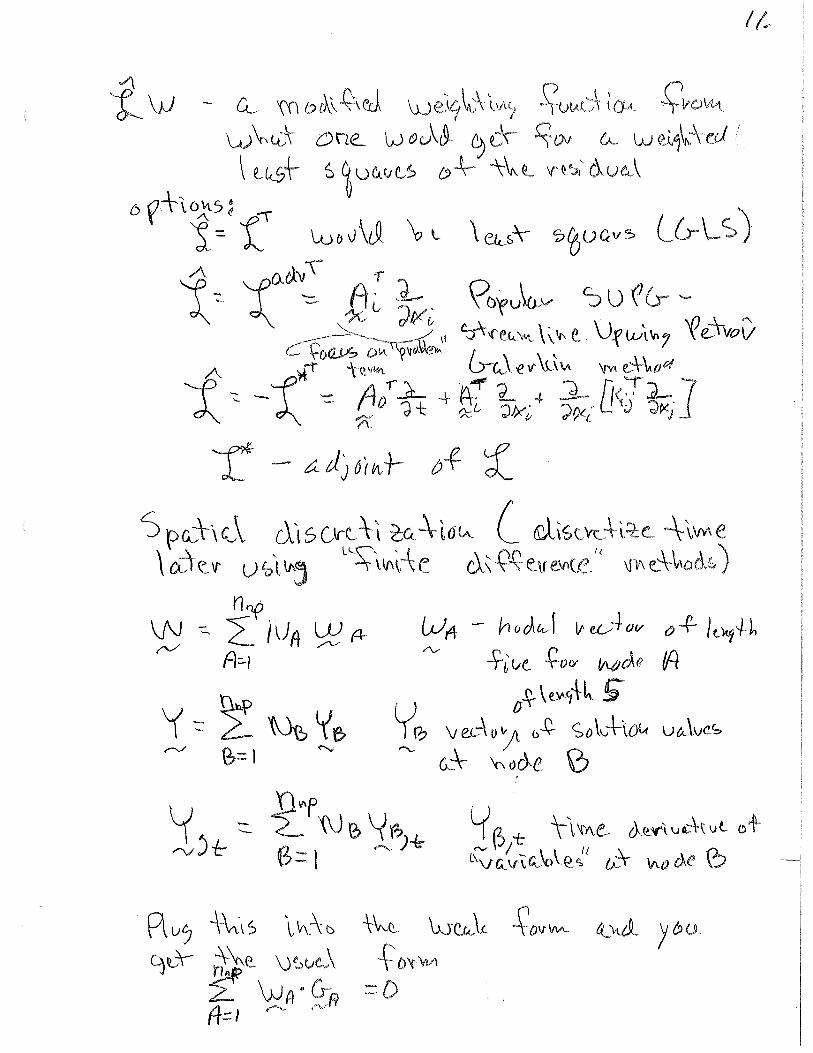
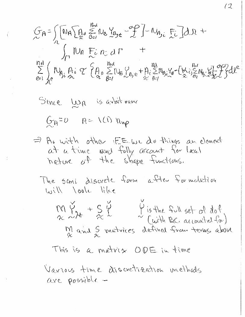
1

Finite Element method for fluid flow problems To this point we have focused on elliptic PDE (only even order derivatives) that produce nice symmetric global systems. Standard Galerkin methods are can be shown to be “optimal” for these problems. On the other hand standard Galerkin methods do not work well for advection dominated problems where there are first derivative terms that are important. One simple advection equation is

φ,t + aiφ,i = 0 in Ω with appropriate boundary and initial conditions. The most basic problem of general interest (that is it has both advection and diffusion) in this class is the “static” advection/diffusion equation

aiφ,i +κφ,ii − f in Ω subject to φ = g on Γ Most problems of interest also have time dependent terms. Since the time domain is almost always handled through semi-discretization (e.g., use finite elements for the spatial discretization and finite difference for the temporal discretization).

If you apply a standard Galerkin finite element method to these equations you will find the solutions will have large oscillations and at large over shoots and undershoots at discontinuities (which can happen in these classes of equations).

Thus a large number of Petrov-Galerkin methods have been developed to address this class of problem. The currently two most popular classes of methods are the:

2

• Discontinuous Galerkin (DG). One Reference (there are a large number of them): Cockburn, Bernardo, George E. Karniadakis, and Chi-Wang Shu. "The development of discontinuous Galerkin methods." In Discontinuous Galerkin Methods, pp. 3-50. Springer, Berlin, Heidelberg, 2000.

• Stabilized finite elements – developed heavily by Tom Hughes (an people that studied with him). There is not a goo book type reference on this method. A few well cited papers are: o Franca, L.P., Frey, S.L. and Hughes, T.J., 1992.

Stabilized finite element methods: I. Application to the advective-diffusive model. Computer Methods in Applied Mechanics and Engineering, 95(2), pp.253-276.

o Franca, L.P. and Frey, S.L., 1992. Stabilized finite element methods: II. The incompressible Navier-Stokes equations. Computer Methods in Applied Mechanics and Engineering, 99(2-3), pp.209-233.

o Tezduyar, T.E., 1991. Stabilized finite element formulations for incompressible flow computations. In Advances in applied mechanics (Vol. 28, pp. 1-44). Elsevier.

o Whiting, C.H. and Jansen, K.E., 2001. A stabilized finite element method for the incompressible Navier–Stokes equations using a hierarchical basis. International Journal for Numerical Methods in Fluids, 35(1), pp.93-116.

How do we achieve this ?

Let us consider a few well known schemes and their basic properties to understand what is needed.

Consider the basic equation

All schemes involve two choices

• In which way does one approximate the solution ?• In which way should the approximation satisfy the PDE ?

1

Introduction

When faced with the task of solving a partial differential equation computa-tionally, one quickly realizes that there is quite a number of different methodsfor doing so. Among these are the widely used finite difference, finite ele-ment, and finite volume methods, which are all techniques used to derivediscrete representations of the spatial derivative operators. If one also needsto advance the equations in time, there is likewise a wide variety of methodsfor the integration of systems of ordinary differential equations available tochoose among. With such a variety of successful and well tested methods, oneis tempted to ask why there is a need to consider yet another method.

To appreciate this, let us begin by attempting to understand the strengthsand weaknesses of the standard techniques. We consider the one-dimensionalscalar conservation law for the solution u(x, t)

∂u

∂t+

∂f

∂x= g, x ∈ Ω, (1.1)

subject to an appropriate set of initial conditions and boundary conditions onthe boundary, ∂Ω. Here f(u) is the flux, and g(x, t) is some prescribed forcingfunction.

The construction of any numerical method for solving a partial differentialequation requires one to consider the two choices:

• How does one represent the solution u(x, t) by an approximate solutionuh(x, t)?

• In which sense will the approximate solution uh(x, t) satisfy the partialdifferential equation?

These two choices separate the different methods and define the properties ofthe methods. It is instructive to seek a detailed understanding of these choicesand how they impact the schemes to appreciate how to address problems andlimitations associated with the classic schemes.

Let us begin with the simplest and historically oldest method, known asthe finite difference method. In this approach, a grid, xk, k = 1 . . . K, is laid

Finite difference methods

• The local approximation is a 1D polynomial• The equation is satisfied in a pointwise manner

2 1 Introduction

down in space and spatial derivatives are approximated by difference methods;that is, the conservation law is approximated as

duh(xk, t)dt

+fh(xk+1, t) − fh(xk−1, t)

hk + hk−1= g(xk, t), (1.2)

where uh and fh are the numerical approximations to the solution and theflux, respectively, and hk = xk+1 − xk is the local grid size. The constructionof a finite difference method requires that, in the neighborhood of each gridpoint xk, the solution and the flux are assumed to be well approximated bylocal polynomials

x ∈ [xk−1, xk+1] : uh(x, t) =2∑

i=0

ai(t)(x− xk)i, fh(x, t) =2∑

i=0

bi(t)(x− xk)i,

where the coefficients ai(t) and bi(t) are found by requiring that the approx-imate function interpolates at the grid points, xk. Inserting these local ap-proximations into Eq. (1.1), results in the residual

x ∈ [xk−1, xk+1] : Rh(x, t) =∂uh

∂t+

∂fh

∂x− g(x, t).

Clearly, Rh(x, t) is not zero, as in that case, uh(x, t) would satisfy Eq. (1.1)exactly and would be the solution u(x, t). Thus, we need to specify in whichway uh must satisfy the equation, which amounts to a statement about theresidual, Rh(x, t). If we have a total of K grid points and, thus, K unknowngrid point values, uh(xk, t), a natural choice is to require that the residualvanishes exactly at these grid points. This results in exactly K finite differenceequations of the type in Eq. (1.2) for the K unknowns, completing the scheme.

One of the most appealing aspects of this method is its simplicity; thatis the discretization of general problems and operators is often intuitive and,for many problems, leads to very efficient schemes. Furthermore, the explicitsemidiscrete form gives flexibility in the choice of timestepping methods ifneeded. Finally, these methods are supported by an extensive body of theory(see, e.g., [142]), they are sufficiently robust and efficient to be used for avariety of problems, and extensions to higher order approximations by using alocal polynomial approximation of higher degree is relatively straightforward.

It is also, however, the reliance on the local one-dimensional polynomialapproximation that is the Achilles’ heel of the method, as that enforces a sim-ple dimension-by-dimension structure in higher dimensions. Additional com-plications caused by the simple underlying structure are introduced aroundboundaries and discontinuous internal layers (e.g., discontinuous material co-efficients). This makes the native finite difference method ill-suited to dealwith complex geometries, both in terms of general computational domainsand internal discontinuities as well as for local order and grid size changes toreflect local features of the solution.

2 1 Introduction

that, in the neighborhood of each grid point xk, the solution and the flux are assumed to be wellapproximated by local polynomials

x [xk1, xk+1] : uh(x, t) =2

i=0

ai(t)(x xk)i, fh(x, t) =2

i=0

bi(t)(x xk)i,

where the coecients ai(t) and bi(t) are found by requiring that the approximate function inter-polates at the grid points, xk. Inserting these local approximations into Eq.(1.1), results in theresidual

x [xk1, xk+1] : Rh(x, t) =uh

t+

fh

x g(x, t).

Clearly, Rh(x, t) is not zero, as in that case, uh(x, t) would satisfy Eq.(1.1) exactly and wouldbe the solution u(x, t). Thus, we must specify in which way uh must satisfy the equation, whichamounts to a statement about the residual, Rh(x, t). If we have a total of Np grid points and, thus,Np unknown grid point values, uh(xk, t), a natural choice is to require that the residual vanishesexactly at these grid points. This results in exactly Np finite dierence equations of the type inEq.(1.2) for the Np unknowns, completing the scheme.

One of the most appealing aspects of this method is its simplicity; that is the discretization ofgeneral problems and operators is often intuitive and, for many problems, leads to very ecientschemes. Furthermore, the explicit semidiscrete form gives flexibility in the choice of timesteppingmethods if needed. Finally, these methods are supported by an extensive body of theory (see, e.g.,[142]), they are suciently robust and ecient to be used for a variety of problems, and extensionsto higher order approximations by using a local polynomial approximation of higher degree isrelatively straightforward.

It is also, however, the reliance on the local one-dimensional polynomial approximation thatis the Achilles’ heel of the method, as that enforces a simple dimension-by-dimension structurein higher dimensions. Additional complications caused by the simple underlying structure are in-troduced around boundaries and discontinuous internal layers (e.g., discontinuous material coe-cients). This makes the native finite dierence method ill-suited to deal with complex geometries,both in terms of general computational domains and internal discontinuities as well as for localorder and grid size changes to reflect local features of the solution.

The above discussion highlights that to ensure geometric flexibility one needs to abandon thesimple one-dimensional approximation in favor of something more general. The most natural is tointroduce an element-based discretization. Hence, we assume that is represented by a collection ofelements, Dk, typically simplexes or cubes, organized in an unstructured manner to fill the physicaldomain.

A method closely related to the finite dierence method, but with added geometric flexibility, isthe finite volume method. In its simplest form, the solution u(x, t) is approximated on the elementby a constant, uk(t), at the center, xk, of the element. This is introduced into Eq.(1.1) to recoverthe cellwise residual

x Dk : Rh(x, t) =uk

t+

f(uk)x

g(x, t),

where the element is defined as D=[xk1/2, xk+1/2] with xk+1/2 = 12 (xk +xk+1). In the finite volume

method we require that the cell average of the residual vanishes identically, leading to the scheme

2 1 Introduction

that, in the neighborhood of each grid point xk, the solution and the flux are assumed to be wellapproximated by local polynomials

x [xk1, xk+1] : uh(x, t) =2

i=0

ai(t)(x xk)i, fh(x, t) =2

i=0

bi(t)(x xk)i,

where the coecients ai(t) and bi(t) are found by requiring that the approximate function inter-polates at the grid points, xk. Inserting these local approximations into Eq.(1.1), results in theresidual

x [xk1, xk+1] : Rh(x, t) =uh

t+

fh

x g(x, t).

Clearly, Rh(x, t) is not zero, as in that case, uh(x, t) would satisfy Eq.(1.1) exactly and wouldbe the solution u(x, t). Thus, we must specify in which way uh must satisfy the equation, whichamounts to a statement about the residual, Rh(x, t). If we have a total of Np grid points and, thus,Np unknown grid point values, uh(xk, t), a natural choice is to require that the residual vanishesexactly at these grid points. This results in exactly Np finite dierence equations of the type inEq.(1.2) for the Np unknowns, completing the scheme.

One of the most appealing aspects of this method is its simplicity; that is the discretization ofgeneral problems and operators is often intuitive and, for many problems, leads to very ecientschemes. Furthermore, the explicit semidiscrete form gives flexibility in the choice of timesteppingmethods if needed. Finally, these methods are supported by an extensive body of theory (see, e.g.,[142]), they are suciently robust and ecient to be used for a variety of problems, and extensionsto higher order approximations by using a local polynomial approximation of higher degree isrelatively straightforward.

It is also, however, the reliance on the local one-dimensional polynomial approximation thatis the Achilles’ heel of the method, as that enforces a simple dimension-by-dimension structurein higher dimensions. Additional complications caused by the simple underlying structure are in-troduced around boundaries and discontinuous internal layers (e.g., discontinuous material coe-cients). This makes the native finite dierence method ill-suited to deal with complex geometries,both in terms of general computational domains and internal discontinuities as well as for localorder and grid size changes to reflect local features of the solution.

The above discussion highlights that to ensure geometric flexibility one needs to abandon thesimple one-dimensional approximation in favor of something more general. The most natural is tointroduce an element-based discretization. Hence, we assume that is represented by a collection ofelements, Dk, typically simplexes or cubes, organized in an unstructured manner to fill the physicaldomain.

A method closely related to the finite dierence method, but with added geometric flexibility, isthe finite volume method. In its simplest form, the solution u(x, t) is approximated on the elementby a constant, uk(t), at the center, xk, of the element. This is introduced into Eq.(1.1) to recoverthe cellwise residual

x Dk : Rh(x, t) =uk

t+

f(uk)x

g(x, t),

where the element is defined as D=[xk1/2, xk+1/2] with xk+1/2 = 12 (xk +xk+1). In the finite volume

method we require that the cell average of the residual vanishes identically, leading to the scheme

Finite difference schemes

• Main benefits• Simple to implement and fast• High-order is feasible• Explicit in time• Direction can be exploited - upwind• Strong theory

• Main problem• Simple local approximation and geometric flexibility are not agreeable

Finite volume methods

• The local approximation is a cell average

• The equation is satisfied on conservation form

1 Introduction 3

The above discussion highlights that to ensure geometric flexibility oneneeds to abandon the simple one-dimensional approximation in favor of some-thing more general. The most natural approach is to introduce an element-based discretization. Hence, we assume that Ω is represented by a collectionof elements, Dk, typically simplexes or cubes, organized in an unstructuredmanner to fill the physical domain.

A method closely related to the finite difference method, but with addedgeometric flexibility, is the finite volume method. In its simplest form, thesolution u(x, t) is approximated on the element by a constant, uk(t), at thecenter, xk, of the element. This is introduced into Eq. (1.1) to recover thecellwise residual

x ∈ Dk : Rh(x, t) =∂uk

∂t+

∂f(uk)∂x

− g(x, t),

where the element is defined as Dk = [xk−1/2, xk+1/2] with xk+1/2 = 12 (xk +

xk+1). In the finite volume method we require that the cell average of theresidual vanishes identically, leading to the scheme

hk duk

dt+ fk+1/2 − fk−1/2 = hkgk, (1.3)

for each cell. Note that the approximation and the scheme is purely localand, thus, imposes no conditions on the grid structure. In particular, all cellscan have different sizes, hk. The flux term reduces to a pure surface termby the use of the divergence theorem, also known as Gauss’ theorem. Thisstep introduces the need to evaluate the fluxes at the boundaries. However,since our unknowns are the cell averages of the numerical solution uh, theevaluation of these fluxes is not straightforward.

This reconstruction problem and the subsequent evaluation of the fluxes atthe interfaces can be addressed in many different ways and the details of thislead to different finite volume methods. A simple solution to the reconstructionproblem is to use

uk+1/2 =uk+1 + uk

2, fk+1/2 = f(uk+1/2),

and likewise for fk−1/2. Alternatively, one could be tempted to simply take

fk+1/2 =f(uk) + f(uk+1)

2,

although this turns out to not be a good idea for general nonlinear problems.For linear problems and equidistant grids these methods all reduce to the finitedifference method. However, one easily realizes that the formulation is lessrestrictive in terms of the grid structure; that is, the reconstruction of solutionvalues at the interfaces is a local procedure and generalizes straightforwardlyto unstructured grids in high dimensions, thus ensuring the desired geometric

1 Introduction 3

hk duk

dt+ fk+1/2 fk1/2 = hkgk, (1.3)

for each cell. Note that the approximation and the scheme is purely local and, thus, imposes noconditions on the grid structure. In particular, all cells can have dierent sizes, hk. The flux termreduces to a pure surface term by the use of the divergence theorem, also known as Gauss’ the-orem. This step introduces the need to evaluate the fluxes at the boundaries. However, since ourunknowns are the cell averages of the numerical solution uh, the evaluation of these fluxes is notstraightforward.

This reconstruction problem and the subsequent evaluation of the fluxes at the interfaces canbe addressed in many dierent ways and the details of this lead to dierent finite volume methods.A simple and natural solution to the reconstruction problem is to use

uk+1/2 =uk+1 + uk

2, fk+1/2 = f(uk+1/2),

and likewise for fk1/2. Alternatively, one could be tempted to simply take

fk+1/2 =f(uk) + f(uk+1)

2,

although this turns out to not be a good idea for general nonlinear problems. For linear problemsand equidistant grids these methods all reduce to the finite dierence method. However, one easilyrealizes that the formulation is less restrictive in terms of the grid structure; that is, the recon-struction of solution values at the interfaces is a local procedure and generalizes straightforwardlyto unstructured grids in high dimensions, thus ensuring the desired geometric flexibility. Further-more, the construction of the interface fluxes can be done in various ways that are closely relatedto the particular equations (see, e.g., [218, 303]). This is particularly powerful when one considersnonlinear conservation laws.

If, however, we wish to increase the order of accuracy of the method, a fundamental problememerges. Consider again the problem in one dimension. We wish to reconstruct the solution, uh, atthe interface and we seek a local polynomial, uh(x) of the form

x [xk1/2, xk+3/2] : uh(x) = a + bx.

We then require

xk+1/2

xk1/2uh(x) dx = hkuk,

xk+3/2

xk+1/2uh(x) dx = hk+1uk+1

to recover the two coecients. The reconstructed value of the solution, uh, and therefore alsof(uh(xk+1/2)) can then be evaluated.

To reconstruct the interface values at a higher accuracy we can continue as above and seek alocal solution of the form

uh(x) =p

j=0

aj(x xk)j .

1 Introduction 3

hk duk

dt+ fk+1/2 fk1/2 = hkgk, (1.3)

for each cell. Note that the approximation and the scheme is purely local and, thus, imposes noconditions on the grid structure. In particular, all cells can have dierent sizes, hk. The flux termreduces to a pure surface term by the use of the divergence theorem, also known as Gauss’ the-orem. This step introduces the need to evaluate the fluxes at the boundaries. However, since ourunknowns are the cell averages of the numerical solution uh, the evaluation of these fluxes is notstraightforward.

This reconstruction problem and the subsequent evaluation of the fluxes at the interfaces canbe addressed in many dierent ways and the details of this lead to dierent finite volume methods.A simple and natural solution to the reconstruction problem is to use

uk+1/2 =uk+1 + uk

2, fk+1/2 = f(uk+1/2),

and likewise for fk1/2. Alternatively, one could be tempted to simply take

fk+1/2 =f(uk) + f(uk+1)

2,

although this turns out to not be a good idea for general nonlinear problems. For linear problemsand equidistant grids these methods all reduce to the finite dierence method. However, one easilyrealizes that the formulation is less restrictive in terms of the grid structure; that is, the recon-struction of solution values at the interfaces is a local procedure and generalizes straightforwardlyto unstructured grids in high dimensions, thus ensuring the desired geometric flexibility. Further-more, the construction of the interface fluxes can be done in various ways that are closely relatedto the particular equations (see, e.g., [218, 303]). This is particularly powerful when one considersnonlinear conservation laws.

If, however, we wish to increase the order of accuracy of the method, a fundamental problememerges. Consider again the problem in one dimension. We wish to reconstruct the solution, uh, atthe interface and we seek a local polynomial, uh(x) of the form

x [xk1/2, xk+3/2] : uh(x) = a + bx.

We then require

xk+1/2

xk1/2uh(x) dx = hkuk,

xk+3/2

xk+1/2uh(x) dx = hk+1uk+1

to recover the two coecients. The reconstructed value of the solution, uh, and therefore alsof(uh(xk+1/2)) can then be evaluated.

To reconstruct the interface values at a higher accuracy we can continue as above and seek alocal solution of the form

uh(x) =p

j=0

aj(x xk)j .

1 Introduction 3

hk duk

dt+ fk+1/2 fk1/2 = hkgk, (1.3)

for each cell. Note that the approximation and the scheme is purely local and, thus, imposes noconditions on the grid structure. In particular, all cells can have dierent sizes, hk. The flux termreduces to a pure surface term by the use of the divergence theorem, also known as Gauss’ the-orem. This step introduces the need to evaluate the fluxes at the boundaries. However, since ourunknowns are the cell averages of the numerical solution uh, the evaluation of these fluxes is notstraightforward.

This reconstruction problem and the subsequent evaluation of the fluxes at the interfaces canbe addressed in many dierent ways and the details of this lead to dierent finite volume methods.A simple and natural solution to the reconstruction problem is to use

uk+1/2 =uk+1 + uk

2, fk+1/2 = f(uk+1/2),

and likewise for fk1/2. Alternatively, one could be tempted to simply take

fk+1/2 =f(uk) + f(uk+1)

2,

although this turns out to not be a good idea for general nonlinear problems. For linear problemsand equidistant grids these methods all reduce to the finite dierence method. However, one easilyrealizes that the formulation is less restrictive in terms of the grid structure; that is, the recon-struction of solution values at the interfaces is a local procedure and generalizes straightforwardlyto unstructured grids in high dimensions, thus ensuring the desired geometric flexibility. Further-more, the construction of the interface fluxes can be done in various ways that are closely relatedto the particular equations (see, e.g., [218, 303]). This is particularly powerful when one considersnonlinear conservation laws.

If, however, we wish to increase the order of accuracy of the method, a fundamental problememerges. Consider again the problem in one dimension. We wish to reconstruct the solution, uh, atthe interface and we seek a local polynomial, uh(x) of the form

x [xk1/2, xk+3/2] : uh(x) = a + bx.

We then require

xk+1/2

xk1/2uh(x) dx = hkuk,

xk+3/2

xk+1/2uh(x) dx = hk+1uk+1

to recover the two coecients. The reconstructed value of the solution, uh, and therefore alsof(uh(xk+1/2)) can then be evaluated.

To reconstruct the interface values at a higher accuracy we can continue as above and seek alocal solution of the form

uh(x) =p

j=0

aj(x xk)j .

Finite volume methods

• Main benefit• Robust and fast due to locality• Complex geometries• Well suited for conservation laws• Explicit in time

• Main problem• Inability to achieve high-order on general grids due to extended stencils• Grid smoothness requirements

1 Introduction 3

The above discussion highlights that to ensure geometric flexibility oneneeds to abandon the simple one-dimensional approximation in favor of some-thing more general. The most natural approach is to introduce an element-based discretization. Hence, we assume that Ω is represented by a collectionof elements, Dk, typically simplexes or cubes, organized in an unstructuredmanner to fill the physical domain.

A method closely related to the finite difference method, but with addedgeometric flexibility, is the finite volume method. In its simplest form, thesolution u(x, t) is approximated on the element by a constant, uk(t), at thecenter, xk, of the element. This is introduced into Eq. (1.1) to recover thecellwise residual

x ∈ Dk : Rh(x, t) =∂uk

∂t+

∂f(uk)∂x

− g(x, t),

where the element is defined as Dk = [xk−1/2, xk+1/2] with xk+1/2 = 12 (xk +

xk+1). In the finite volume method we require that the cell average of theresidual vanishes identically, leading to the scheme

hk duk

dt+ fk+1/2 − fk−1/2 = hkgk, (1.3)

for each cell. Note that the approximation and the scheme is purely localand, thus, imposes no conditions on the grid structure. In particular, all cellscan have different sizes, hk. The flux term reduces to a pure surface termby the use of the divergence theorem, also known as Gauss’ theorem. Thisstep introduces the need to evaluate the fluxes at the boundaries. However,since our unknowns are the cell averages of the numerical solution uh, theevaluation of these fluxes is not straightforward.

This reconstruction problem and the subsequent evaluation of the fluxes atthe interfaces can be addressed in many different ways and the details of thislead to different finite volume methods. A simple solution to the reconstructionproblem is to use

uk+1/2 =uk+1 + uk

2, fk+1/2 = f(uk+1/2),

and likewise for fk−1/2. Alternatively, one could be tempted to simply take

fk+1/2 =f(uk) + f(uk+1)

2,

although this turns out to not be a good idea for general nonlinear problems.For linear problems and equidistant grids these methods all reduce to the finitedifference method. However, one easily realizes that the formulation is lessrestrictive in terms of the grid structure; that is, the reconstruction of solutionvalues at the interfaces is a local procedure and generalizes straightforwardlyto unstructured grids in high dimensions, thus ensuring the desired geometric

The key challenge is one of reconstruction

Finite element methods

We begin by splitting the solution into elements as

• The solution is defined in a nonlocal manner

• The equation is satisfied globally

1 Introduction 5

x ∈ Dk : uh(x) =Np∑

n=1

bnψn(x),

where we have introduced the use of a locally defined basis function, ψn(x).In the simplest case, we can take these basis functions be linear; that is,

x ∈ Dk : uh(x) = u(xk)x − xk+1

xk − xk+1+ u(xk+1)

x − xk

xk+1 − xk=

1∑

i=0

u(xk+i)ℓki (x),

where the linear Lagrange polynomial, ℓki (x), is given as

ℓki (x) =

x − xk+1−i

xk+i − xk+1−i.

With this local element-based model, each element shares the nodes with oneother element (e.g., Dk−1 and Dk share xk). We have a global representationof uh as

uh(x) =K∑

k=1

u(xk)Nk(x) =K∑

k=1

ukNk(x),

where the piecewise linear shape function, N i(xj) = δij is the basis functionand uk = u(xk) remain as the unknowns.

To recover the scheme to solve Eq. (1.1), we define a space of test functions,Vh, and require that the residual is orthogonal to all test functions in thisspace as

∫

Ω

(∂uh

∂t+

∂fh

∂x− gh

)φh(x) dx = 0, ∀φh ∈ Vh.

The details of the scheme is determined by how this space of test functions isdefined. A classic choice, leading to a Galerkin scheme, is to require the thatspaces spanned by the basis functions and test functions are the same. In thisparticular case we thus assume that

φh(x) =K∑

k=1

v(xk)Nk(x).

Since the residual has to vanish for all φh ∈ Vh, this amounts to∫

Ω

(∂uh

∂t+

∂fh

∂x− gh

)N j(x) dx = 0,

for j = 1 . . . K. Straightforward manipulations yield the scheme

Mduh

dt+ Sfh = Mgh, (1.4)

1 Introduction 5

x ∈ Dk : uh(x) =Np∑

n=1

bnψn(x),

where we have introduced the use of a locally defined basis function, ψn(x).In the simplest case, we can take these basis functions be linear; that is,

x ∈ Dk : uh(x) = u(xk)x − xk+1

xk − xk+1+ u(xk+1)

x − xk

xk+1 − xk=

1∑

i=0

u(xk+i)ℓki (x),

where the linear Lagrange polynomial, ℓki (x), is given as

ℓki (x) =

x − xk+1−i

xk+i − xk+1−i.

With this local element-based model, each element shares the nodes with oneother element (e.g., Dk−1 and Dk share xk). We have a global representationof uh as

uh(x) =K∑

k=1

u(xk)Nk(x) =K∑

k=1

ukNk(x),

where the piecewise linear shape function, N i(xj) = δij is the basis functionand uk = u(xk) remain as the unknowns.

To recover the scheme to solve Eq. (1.1), we define a space of test functions,Vh, and require that the residual is orthogonal to all test functions in thisspace as

∫

Ω

(∂uh

∂t+

∂fh

∂x− gh

)φh(x) dx = 0, ∀φh ∈ Vh.

The details of the scheme is determined by how this space of test functions isdefined. A classic choice, leading to a Galerkin scheme, is to require the thatspaces spanned by the basis functions and test functions are the same. In thisparticular case we thus assume that

φh(x) =K∑

k=1

v(xk)Nk(x).

Since the residual has to vanish for all φh ∈ Vh, this amounts to∫

Ω

(∂uh

∂t+

∂fh

∂x− gh

)N j(x) dx = 0,

for j = 1 . . . K. Straightforward manipulations yield the scheme

Mduh

dt+ Sfh = Mgh, (1.4)

Finite element methods

1 Introduction 5

x ∈ Dk : uh(x) =Np∑

n=1

bnψn(x),

where we have introduced the use of a locally defined basis function, ψn(x).In the simplest case, we can take these basis functions be linear; that is,

x ∈ Dk : uh(x) = u(xk)x − xk+1

xk − xk+1+ u(xk+1)

x − xk

xk+1 − xk=

1∑

i=0

u(xk+i)ℓki (x),

where the linear Lagrange polynomial, ℓki (x), is given as

ℓki (x) =

x − xk+1−i

xk+i − xk+1−i.

With this local element-based model, each element shares the nodes with oneother element (e.g., Dk−1 and Dk share xk). We have a global representationof uh as

uh(x) =K∑

k=1

u(xk)Nk(x) =K∑

k=1

ukNk(x),

where the piecewise linear shape function, N i(xj) = δij is the basis functionand uk = u(xk) remain as the unknowns.

To recover the scheme to solve Eq. (1.1), we define a space of test functions,Vh, and require that the residual is orthogonal to all test functions in thisspace as

∫

Ω

(∂uh

∂t+

∂fh

∂x− gh

)φh(x) dx = 0, ∀φh ∈ Vh.

The details of the scheme is determined by how this space of test functions isdefined. A classic choice, leading to a Galerkin scheme, is to require the thatspaces spanned by the basis functions and test functions are the same. In thisparticular case we thus assume that

φh(x) =K∑

k=1

v(xk)Nk(x).

Since the residual has to vanish for all φh ∈ Vh, this amounts to∫

Ω

(∂uh

∂t+

∂fh

∂x− gh

)N j(x) dx = 0,

for j = 1 . . . K. Straightforward manipulations yield the scheme

Mduh

dt+ Sfh = Mgh, (1.4)

• Main benefits• High-order accuracy and complex geometries can be combined

• Main problems• Implicit in time• Not well suited for problems with direction

This yields the global equation

1 Introduction 5

h(x) =K

k=1

v(xk)Nk(x).

Since the residual has to vanish for all h Vh, this amounts to

uh

t+

fh

x gh

N j(x) dx = 0,

for j = 1 . . .K. Straightforward manipulations yield the scheme

Mduh

dt+ Sfh =Mgh, (1.4)

where

Mij =

N i(x)N j(x) dx, Sij =

N i(x)

dN j

dxdx,

reflects the globally defined mass matrix and stiness matrix, respectively. We also have thevectors of unknowns, uh = [u1, . . . , uNp ]T , of fluxes, fh = [f1, . . . , fNp ]T , and the forcing,gh = [g1, . . . , gNp ]T , given on the Np nodes.

This approach, which reflects the essence of the classic finite element method [182, 339, 340, 341],clearly allows dierent element sizes. Furthermore, we recall that a main motivation for consideringmethods beyond the finite volume approach was the interest in higher-order approximations. Suchextensions are relatively simple in the finite element setting and can be achieved by adding additionaldegrees of freedom to the element while maintaining shared nodes along the faces of the elements[197]. In particular, one can have dierent orders of approximation in each element, thereby enablinglocal changes in both size and order, known as hp-adaptivity (see, e.g., [93, 94]).

However, the above discussion also highlights disadvantages of the classic continuous finite ele-ment formulation. First, we see that the globally defined basis functions and the requirement thatthe residual be orthogonal to same set of globally defined test functions implies that the semidis-crete scheme becomes implicit and M must be inverted. For time dependent problems, this is aclear disadvantage compared to finite dierence and finite volume methods. On the other hand, forproblems with no explicit time dependence, this is less of a concern.

There is an additional subtle issue that relates to the structure of the basis. If we recall thediscussion above, we recognize that the basis functions are symmetric in space. For many typesof problems (e.g., a heat equation), this is a natural choice. However, for problems such as waveproblems and conservation laws, in which information flows in specific directions, this is less naturaland can causes stability problems if left unchanged (see, e.g., [182, 339]). In finite dierence andfinite volume methods, this problem is addressed by the use of upwinding, either through the stencilchoice or through the design of the reconstruction approach.

In Table 1.1 we summarize some of the issues discussed so far. Looking at it, one should keepin mind that this comparison reflects the most basic methods and that many of the problemsand restrictions can be addressed and overcome in a variety of ways. Nevertheless, the comparisondoes highlight which shortcoming one should strive to resolve when attempting to formulate a newmethod.

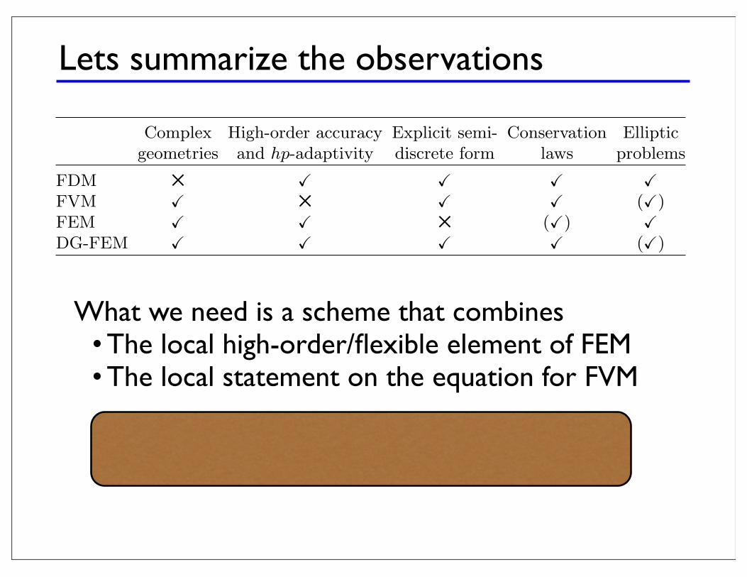
Lets summarize the observations

1 Introduction 7

Table 1.1. We summarize generic properties of the most widely used methods fordiscretizing partial differential equations [i.e., finite difference methods (FDM), finitevolume methods (FVM), and finite element methods (FEM), as compared with thediscontinuous Galerkin finite element method (DG-FEM)]. A ! represents success,while indicates a short-coming in the method. Finally, a (!) reflects that themethod, with modifications, is capable of solving such problems but remains a lessnatural choice.

Complex High-order accuracy Explicit semi- Conservation Ellipticgeometries and hp-adaptivity discrete form laws problems

FDM ! ! ! !FVM ! ! ! (!)FEM ! ! (!) !DG-FEM ! ! ! ! (!)

residual destroys the locality of the scheme and introduces potential problemswith the stability for wave-dominated problems. On the other hand, this isprecisely the regime where the finite volume method has several attractivefeatures.

An intelligent combination of the finite element and the finite volumemethods, utilizing a space of basis and test functions that mimics the finiteelement method but satisfying the equation in a sense closer to the finitevolume method, appears to offer many of the desired properties. This com-bination is exactly what leads to the discontinuous Galerkin finite elementmethod (DG-FEM).

To achieve this, we maintain the definition of elements as in the finiteelement scheme such that Dk = [xk, xk+1]. However, to ensure the localityof the scheme, we duplicate the variables located at the nodes xk. Hence thevector of unknowns is defined as

uh = [u1, u2, u2, u3, . . . , uK−1, uK , uK , uK+1]T ,

and is now 2K long rather than K + 1 as in the finite element method. Ineach of these elements we assume that the local solution can be expressed as

x ∈ Dk : ukh(x) = uk x − xk+1

xk − xk+1+ uk+1 x − xk

xk+1 − xk=

1∑

i=0

uk+iℓki (x) ∈ Vh,

and likewise for the flux, fkh . The space of basis functions is defined as Vh =

⊕Kk=1

ℓki

1

i=0, i.e., as the space of piecewise polynomial functions. Note in

particular that there is no restrictions on the smoothness of the basis functionsbetween elements.

As in the finite element case, we now assume that the local solution canbe well represented by a linear approximation uh ∈ Vh and form the localresidual

What we need is a scheme that combines• The local high-order/flexible element of FEM• The local statement on the equation for FVM

These are exactly the components of the Discontinuous Galerkin Finite Element Method