Finite Element Analysis of the Time-Dependent …ccom.ucsd.edu/~mholst/pubs/dist/CSZB06.pdf ·...

Time-Dependent Smoluchowski Solver 1

Finite Element Analysis of the Time-DependentSmoluchowski Equation for Acetylcholinesterase Reaction

Rate Calculations

Yuhui Cheng∗1, Jason K. Suen

, Deqiang Zhang§, Stephen D. Bond

, Yongjie

Zhang¶, Yuhua Song∗∗, Nathan A. Baker∗∗, Chandrajit L. Bajaj¶‖, Michael J.Holst§§ and J. Andrew McCammon∗

∗Howard Hughes Medical Institute, Department of Chemistry and Biochemistry, andCenter for Theoretical Biological Physics, Department of Pharmacology, §§Department

of Mathematics, University of California, San Diego, La Jolla, CA92093-0365;§Accelrys,Inc., 10188 Telesis Court, Suite 100, San Diego, CA 92121-4779; Department of

Computer Science, University of Illinois at Urbana-Champaign, Urbana, IL61801;¶Institute of Computational Engineering and Sciences, Center for ComputationalVisualization,‖Department of Computer Sciences, University of Texas at Austin, Texas

78712; and∗∗Department of Biochemistry and Molecular Biophysics, Center forComputational Biology, Washington University in St. Louis, Missouri 63110

1Corresponding author. Address: Department of Chemistry and Biochemistry, University ofCalifornia, San Diego, 9500 Gilman Dr. MC 0365, La Jolla, CA 92093-0365, U.S.A., Tel.: (858)822-2771, Fax: (858)534-4974

Abstract

This article describes the numerical solution of the time-dependent Smoluchowskiequation to study diffusion in biomolecular systems. Specifically, finite elementmethods have been developed to calculate ligand binding rate constants for largebiomolecules. The resulting software has been validated and applied to the mouseacetylcholinesterase monomer and several tetramers. Rates for inhibitor bindingto mAChE were calculated at various ionic strengths with several different timesteps. Calculated rates show very good agreement with experimental and the-oretical steady-state studies. Furthermore, these finite element methods requiresignificantly fewer computational resources than existing particle-based Browniandynamics methods and are robust for complicated geometries. The key finding ofbiological importance is that the rate accelerations of the monomeric and tetramericmAChE that result from electrostatic steering are preserved under the non-steady-state conditions that are expected to occur in physiological circumstances.

Key words: Finite element method; Smoluchowski equation; Time-dependentdiffusion


IntroductionDiffusion plays an important role in a variety of biomolecular processes, whichhave been studied extensively using various biophysical, biochemical and compu-tational methods. Computational models of diffusion have been widely studiedusing both discrete (1–5) and continuum methods (6–11). The discrete meth-ods concentrate on the stochastic processes based on individual particles, whichinclude Monte Carlo(5, 12–14), Brownian dynamics (BD)(15–17) and Langevindynamics(18, 19) simulations. Continuum modeling describes the diffusional pro-cesses via concentration distribution probability in lieu of stochastic dynamics ofindividual particles. Comparing with the discrete methods, continuum approachesneedn’t deal with the individual Brownian particles and the computionational costcan be substantially less than for the discrete methods.

In previous work with continuum methods, Song et al. have presented finiteelement methods for solving the Steady-State Smoluchowski equation (SSSE),which describes the steady-state behavior of diffusion-limited ligand binding(9,10). These methods have been shown to be significantly more efficient than tradi-tional Brownian dynamics (BD) approaches for evaluating reaction rate constantsfor diffusion-limited binding of simple ligands. Recently, Zhang et al. appliedthis approach for studies of several conformations of tetrameric mouse acetyl-cholinesterase (mAChE)(20). However, the SSSE solution only provides the an-swer at the time independent stage of diffusion. In other words, we only obtainthe concentration distribution and rate constant when diffusion and reaction be-tween the ligand and the enzyme reach the steady state. Physiological conditions,however, can be expected to include nonsteady-state kinetics. One possible way tostudy the diffusion dynamics on biomolecular interface binding energy landscapeis mean first passage time (MFPT), which was introduced recently by Wang et al.(21). The theory suggests a way of connecting the models/simulations with singlemolecule experiments by analyzing the kinetic trajectories. However, it is still anopen question for the diffusional problem in a large spatial and time scale.

In the present work, we apply adaptive finite element methods to solve thetime-dependent Smoluchowski equation (TDSE), using a posteriori error estima-tion to iteratively refine the finite element meshes. The binding of charged andnon-charged ligands to mAChEs has been described at each timestep. The diffu-sion results have been compared with those from steady-state Smoluchowski dif-fusion studies and experimental results. AChE is a serine esterase that terminatesthe activity of acetylcholine (ACh) within cholinergic synapses by hydrolysis ofthe ACh ester bond to produce acetate and choline (22). Hydrolysis of ACh occursin the active site of AChE, which lies at the base of a 20 A-deep gorge within theenzyme. The rate-limiting step of ACh hydrolysis by AChE is the diffusional en-


counter (23–25), making the system a popular target for both experimental (26–28)and computational diffusion studies (29, 30).

Theory and Modeling DetailsOur time-dependent SMOL solver (http://mccammon.ucsd.edu/smol/index.html)models the diffusion of ligands relative to a target molecule, subject to a poten-tial obtained by solving the Poisson-Boltzmann equation. It is perhaps most easilyexplained by initially considering motion of an ensemble of Brownian particles in aprescribed external potential W (~R)(~R being a particle’s position) under conditionsof high friction, where the Smoluchowski equation applies.

Boundaries and Initialization of the Time-Dependent SmoluchowskiEquationThe starting point for development of the time-dependent SMOL solver is thesteady-state SMOL solver described by Song et al. (9, 10). The original Smolu-chowski equation has the form of a continuity equation:

∂p(~R; t)∂t = −~∇ ·~j(~R; t) (1)

where the particle flux is defined as:

~j(~R; t) = D(~R)[~∇p(~R; t)+β~∇W (~R)p(~R; t)]

= D(~R)e−βW (~R)∇eβW (~R)p(~R; t) (2)

Here p(~R; t) is the distribution function of the ensemble of Brownian particles,D(~R) is the diffusion coefficient, β = 1/kBT is the inverse Boltzmann energy, kB isthe Boltzmann constant, T is the temperature, and W (~R) is the potential of meanforce (PMF) for a diffusing particle due to solvent mediated interactions with thetarget molecule. For simplicity, D(~R) can be assumed to be constant. The twoterms contributing to the flux have clear physical meanings. The first is due to freediffusional processes, as quantified by Fick’s first law. The second contributionis due to the drift velocity - ~∇W (~R)γ induced by the systematic forces - ~∇W (~R)and friction quantified by the friction constant γ. The relation beteen diffusioncoefficient D and friction constant γ is given by Stokes-Einstein equation: Dβγ = 1.

The TDSE can be solved to determine biomolecular diffusional encounter ratesbefore steady state is established. Following the work of Song et al.(9, 10) andZhou et al.(31–33), the application of the TDSE to this question involves the solu-


tion of Eq. 1 in a three-dimensional domain Ω, with the following boundary andinitial conditions. A bulk Dirichlet condition is imposed on the outer boundaryΓb ⊂ ∂Ω,

p(~Rl ; t) = pbulk, f or ~Rl ∈ Γb, (3)

where pbulk denotes the bulk concentration at the outer boundary. A reactiveRobin condition is implemented on the active site boundary Γa ⊂ ∂Ω,

n(~R0) ·∇p(~R0; t) = α(~R0)p(~R0), f or ~R0 ∈ Γa, (4)

providing an intrinsic reaction rate α(~R0). Here, n(~R0) is the surface normal. Forthe diffusion-limited reaction process, such as ACh hydrolysis by mAChE, the con-centration of ACh at the binding site is approximately zero. Therefore, the reactiveRobin condition on the inner boundary can be simplified as:

p(~R0; t) = 0, f or ~R0 ∈ Γa, (5)

For the non-reactive surface parts of the inner boundary Γr ⊂ ∂Ω, a reflectiveNeumann condition is employed.

n(~R0) · jp(~R0; t) = 0, (6)

Finally, we set up the initial conditions as

p(~R;0) =

pbulk |~R| = l0 |~R| < l

(7)

Therefore, the diffusion-determined biomolecular reaction rate constant duringthe simulation time can be obtained from the flux ~j(~R; t) by integration over theactive site boundary, i.e.

k(t) = p−1bulk

Z

Γn(~R) ·~j(~R; t)dS (8)


Finite Element Discrete FormulationTo numerically solve the TDSE, we employed the Galerkin finite element approx-imation to discretize the differential equation (34). The original TDSE (eq. 1) canbe written as described below (10, 35, 36):

Let Ω ⊂ R3 be an open set, and let ∂Ω denote the boundary, which can be

thought of as a set in R2. Consider now the TDSE, a member of the class of elliptic

equations:

−∇ · (a(~R; t)∇u(~R; t))+∂p(~R; t)

∂t = 0 in Ω,

p(~R; t) = 0 f or ~R ∈ Γa,

n(~R) · p(~R; t) = 0 f or ~R ∈ Γr,

p(~R; t) = pbulk f or ~R ∈ Γb, (9)

where a(~R; t) = D(~R)e−βW (~R) and u(~R; t) = eβW (~R)p(~R; t).According to Holst et al.(37), the solution to the original problem also solves

the following problem:

Find u ∈ u+H10 (Ω) such that < F(u),v >= 0 ∀v ∈ H1

0 (Ω), (10)

where u is the approximate solution found by the numerical method, u is a tracefunction satisfying the Dirichlet boundary conditions and H 1

0 is the test functionspace (37, 38). The “weak” bilinear form < F(u),v > is given by:

< F(u),v >=

Z

Ω(a∇v ·∇u+

∂u∂t v)dx, (11)

We have used the fact that a boundary integral vanishes due to the fact that thetest function v vanishes on the boundary.

For a discrete solution to eq. 11, taking spanφ1,φ2, ...,φN ⊂ H10 (Ω), eq.

11 reduces to a set of N nonlinear algebraic relations (implicitly defined) for Ncoefficients α j in the expansion:

uh =N∑j=1

α jφ j (12)

According to the Galerkin approximation, N equals the number of finite ele-ment nodes.


Therefore, the corresponding “weak form” of the TDSE is

Find uh − uh ∈ H10 such that < F(uh),vi >= 0 ∀vi ∈ H1

0 , (13)

To obtain an unconditionally stable solution, two implicit algorithms have beenimplemented in our codes: Crank-Nicolson and backward Euler’s methods.

Finally, the concentration distribution can be obtained by p(~R; t)= e−βW (~R)u(~R; t).

0.1 a posteriori Error Estimation and Mesh RefinementAs decribed by Holst et al. (37), the adaptive mesh refinement procedure follows a“solve-estimate-refine” algorithm and has been implemented in the FEtk software(http://www.fetk.org/). Because of the inefficiency to “estimate” and “refine” ineach time step, we only estimated and refined the mesh while solving the SSSE.With the refined mesh, TDSE diffusion studies were implemented. In the “esti-mate” step, we introduced the a posteriori error estimator ηs below holding for aGalerkin approximation uh satisfying

‖u−uh‖H1(Ω) ≤C0∑s∈S

η2s

1/2 (14)

where C0 is a constant and the element-wise error indicator ηs is defined as:

ηs = hs2‖∇ · (a∇uh)‖

2L2(s) +

12 ∑

f∈s‖[n f · (a∇uh)] f ‖

2L2( f )

1/2. (15)

where hs and h f represent the diameter of the simplex s and the face f , respectively.f ∈ s denotes a face of simplex, [v] f denotes the jump across the face of function vand the Lesbegue norm

‖∇ · (a∇uh(r))‖ = De−βW (r)‖∇ ·∇uh(r)−β∇W ·∇uh(r)‖ (16)

The entire “solve-estimate-refine” cycle is repeated until the global error√

∑s η2s

is reduced to an acceptable user-defined level.

Potential of Mean Force (PMF) InputCurrently we provide two options to map the PMF to each finite element node inthe time-dependent SMOL solver code. First, it can input the PMF obtained byboundary element methods (BEM) (39, 40). The PMF corresponds to the elec-trostatic potential obtained by solving the Poisson-Boltzmann equation. Second,APBS 0.4.0 (http://sourceforge.net/projects/apbs) is used to calculate the PMF,


which is the potential field W(r) in Eq. 2 (36). The partial charges and radii ofeach atom in the mAChE monomer and tetramer molecules have been assignedusing the CHARMM22 force field, and the dielectric constant is set as 4.0 insidethe protein and 78.0 for the solvent. The solvent probe radius is set as 1.4 A, andthe ion exclusion layer is set as 2.0 A. Ionic strengths varying between 0 and 0.67M were used in the PMF calculations and following diffusion studies.

To allow the potential to approach zero at the outer boundary, a large space of40 times the radius of the biomolecule is required. A series of nested potential gridsis constructed in a multiresolution format where higher resolution meshes providePMF values near the molecular surface while coarser meshes are used away fromthe molecule. The dimensions of the finest grid are given by the psize.py utilityin the APBS software package, and the coarsest grid dimensions are set to coverthe whole problem domain plus two grid spacings (to allow gradient calculation)in each dimension. The setup for the rest of the grid hierarchy is calculated usinga geometric sequence for grid spacing. For mAChE monomer, the finest grid hasdimensions of 86.3A×76.4A×101.4A with 161, 129 and 193 grid points in eachdirection, respectively. This corresponds to a 0.5A×0.6A×0.5A grid spacing setup.The coarsest grid has dimensions of 3400A×3000A×4300A with 161 grid points ineach direction. The corresponding grid spacing settings are 21.1A×18.6A×26.7A.

Adaptive Finite Element Mesh GenerationFor the mAChE monomer case, similarly with previous studies (9, 10), we used amouse AChE (mAChE) structure adapted from the crystal structure of the mAChE-fasciculin II complex (1MAH) (26) and perturbed by Tara and co-workers viamolecular dynamics simulations with an ACh-like ligand in the active site gorge(30) to produce gorge conformations with wider widths than the original X-raystructure. The diffusing ligand was modeled as a sphere with an exclusion radiusof 2.0 A and a diffusion constant of 7.8×104A2

/µs. This perturbation was neces-sary for computational diffusion simulations with a fixed biomolecular structure.Reactive boundaries were defined using the biomolecular surface, which is exactlythe same with that used in Song et al. (10).

For the mAChE tetramer cases, we used three structures: a loose, pseudosquareplanar tetramer with antiparallel alignment of the two four-helix bundles and a largespace in the center (PDB: 1C2B); a compact, square nonplanar tetramer with par-allel arrangement of the four-helix bundles that may expose all the four t peptidesequences on a single side (PDB: 1C2O); and in addition to the crystal structures,an intermediate structure (INT) was generated by morphing the two crystal struc-tures using the morph script in visual molecular dynamics (41). Reactive boundarydefinitions are exactly the same with the above mAChE monomer case.


The tetrahedral meshes were obtained and refined from the inflated van derWaals-based accessibility data for the mAChE monomer and tetramers using theLevelset Boundary Interior Exterior-Mesher(42–44). Initially the region betweenthe biomolecule and a slightly larger sphere centered about the molecular centerof mass, was discretized by adaptive tetrahedral meshes. It generated very finetriangular elements near the active site gorge, while coarser elements everywhereelse. The mesh is then extended to the entire diffusion domain and the inside of thebiomolecule with spatial adaptivity in that the mesh element size increases withincreasing distance from the biomolecule. The number of tetrahedral elementsvaries from 50,000 to 70,000 for different tetramer geometries.

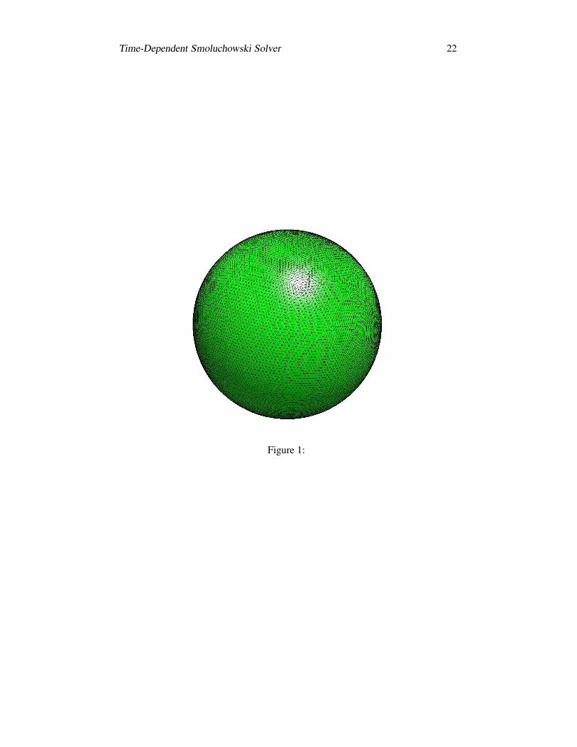
Results and discussionValidation of the Time-Dependent SMOL Code with A Spherical TestCaseBefore applying the time-dependent SMOL program to a biomolecular system withcomplicated geometries, we first tested it with the classic spherical system (45)and compared the calculated result with the known analytical solution. For thistest case, we chose a diffusing sphere with a 2 A radius and neutral charge. Theentire problem domain is a sphere with a 400 A radius, which was discretized with745,472 tetrahedral elements. A detailed view of the surface mesh for the station-ary sphere is also shown in Fig. 1. The time-dependent Smoluchowski equationthen becomes the Einstein diffusion equation. The diffusing particle’s dimension-less bulk concentration was set to 1. Ignoring hydrodynamic interactions, the diffu-sion constant D is calculated as 7.8×104A2

/µs using the Stokes-Einstein equationwith a hydrodynamic radius of 3.5 A, solvent viscosity of 0.891×10−3kg/(m · s),and 300 K temperature.

Analytical solution

For a spherically symmetric system without external potential, the TDSE can bewritten as

∂p∂t = −

1r2

∂∂r (r2J p)

= −1r2

∂∂r (r2D∂p

∂r )


with boundary conditions

p(r0) = pbulk

where r0 is the radius for the outer boundary. The analytical expression for theconcentration distribution is

p(r; t) = pbulk1+2r0πr

∞

∑n=1

(−1)n

n sinnπrr0

exp[−D(nπr0

)2t]

This analytical form of the solution was expressed by the sum of zero-orderspherical Bessel functions. Fig. 2 presents the concentration distributions duringthe simulation time with our TDSE solver, comparing with the above analyticalsolution.

SMOL numerical solution

According to Fig. 2, the performance of the SMOL program is good, with almostthe same concentration distribution as in the analytical solution. It must be notedthat, the analytical solution for the time-dependent diffusion with the Columbic po-tential cannot be addressed with a simple formula, however, we have implementedour solver to test the same steady-state case addressed in Table 1 of Song et al.(10),and obtained very consistent results.

Application of the TDSE Solver to Mouse Acetylcholinesterase MonomerOne of the major advantages of continuum methods such as the time-dependentSMOL solver is the ability to simulate the complete diffusion dynamics for largebiological systems with complicated geometries with significantly lower computa-tional cost than the Brownian dynamics approach. This section demonstrates theimplementation of TDSE to study the ligand binding kinetic process of the mAChEmonomer under various ionic strength conditions (46).

With the original mesh we measured the diffusion-controlled reaction ratesduring the simulation time with the timestep at 50 ps, as shown in Fig. 3. Sep-arate calculations were performed at ionic strengths of 0.000, 0.050, 0.100, 0.150,0.200, 0.250, 0.300, 0.450, 0.600, and 0.670 M. At the zero ionic strength, thewhole system reaches the steady state in over 15 ns. The value of kon at the endof the simulation is 9.535 × 1011M−1 ·min−1, which is very consistent with theexperimental value at (9.80± 0.60)× 1011M−1 ·min−1 (27). Meanwhile, the konvalue for the neutral ligand at the steady state is 9.297× 1010M−1 ·min−1, whichis consistent with the previous steady-state calculations (20). Table 1 listed the fi-


nal kon value derived from the TDSE calculations and the corresponding sets fromSSSE calculations (9). When the ionic strength becomes higher, the time to reachthe steady state decreases substantially. Obviously, we have obtained consistentresults, comparing with the previous SSSE and BD calculations.

Furthermore, our TDSE solver can report all the ligand concentration distribu-tion histories during the 20 µs simulation. In this case, we recorded a concentrationdistribution every 100 timesteps (5 ns) and a restart checkpoint every 1000 timestep(50 ns). Fig. 4 demonstrates the 2D concentration distribution around the mAChEmolecule at the end of 20 µs simulation. The origin and the normal of the clipplane have been set at (0 16.6A 0) and (1 0 1), respectively. kon exhibits an ionicstrength dependence strongly indicative of electrostatistic acceleration. The highionic strength environment lessens the electrostatic interactions between the activesite of mAChE and the ligand. Therefore, the relatively low ligand concentrationarea shrinks while ionic strength increases. Specifically, at 0.150 M ionic strength,several dynamic snapshots have been plotted, as depicted in Fig. 5. These snap-shots demonstrate the whole diffusion process of ACh-like ligands from the areafar from the enzyme until they reach the active site and react and disappear.

In this section, we explore the use of the adaptive finite element methods toimplement TDSE calculations on the mAChE monomer. The first step is to in-teractively solve the SSSE based on the a posteriori error estimation (10, 37). Theiterative error-based refinement of the initial 656,823-simplex mesh was performeduntil the global error is less than a value chosen to provide reaction rates which didnot change appreciably upon further refinement. The refined mesh has 824,746simplices at 150 mM ionic strength. Then, we implemented another TDSE calcu-lations with the refined mesh. Fig. 6 shows the kinetic curves of both the originaland refined mesh. Again, the two calculations are in good overall agreement but doshow some differences at the final steady state. Specifically, the refinement of theadaptive meshes shows a little increase of the kon value after reaching the steadystate.

Application of the TDSE Solver to mAChE TetramersA previous SSSE study described the effect of electrostatic forces on ACh steady-state diffusion to the mouse acetylcholinesterase tetramer (20). Here, we extend theprevious study using the same meshes and potential files with our time-dependentSMOL solver. The time step for the three tetramer models was set at 10 ns, and con-centration histories were recorded every 100 steps. Two crystal structures (1C2Oand 1C2B) and an intermediate structure (INT) are all studied by solving the TDSE.The actual conformational dynamics of the mouse acetylcholinesterase tetramer


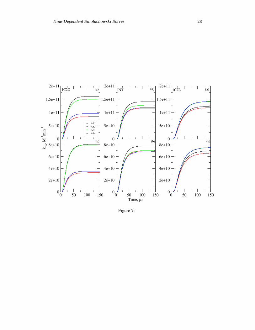
has been neglected in this work.Fig. 7(a) shows the time-dependent rate constant per active site at 0.150 M

ionic strength for the above three mouse acetylcholinesterase tetramer structures.It takes more than 75 µs for each active site to reach the steady state. For structure1C2O, the entrances to two of the four active gorges (AS2 and AS4) are partiallyblocked by another subunit in the complementary dimer, while the other two gorgesare completely accessible from outside (AS1 and AS3). As a result, the four kineticcurves in 1C2O can be classified into two subgroups: one subgroup corresponds toactive site 1 (AS1) and active site 3 (AS3), in each of which the gorge is open, andat the end of the simulation, the reaction rates are 1.61×1011M−1min−1 and 1.50×1011M−1min−1, respectively; another subgroup corresponds to active site 2 (AS2)and active site 4 (AS3), where the gorges are sterically shielded by nearby subunits,and the final reaction rates are 8.47× 1010M−1min−1 and 9.62× 1010M−1min−1,respectively, which is a little more than half of that for AS1 or AS3. Fig. 7(b)demonstrates the kon(t) values for the neutral ligand. Comparing with the +1.0echarged ligand, the neutral ligand still shows similar time-dependent curves forindividual active sites, while the kon(t) value is much less than the corresponding+1.0e charged case.

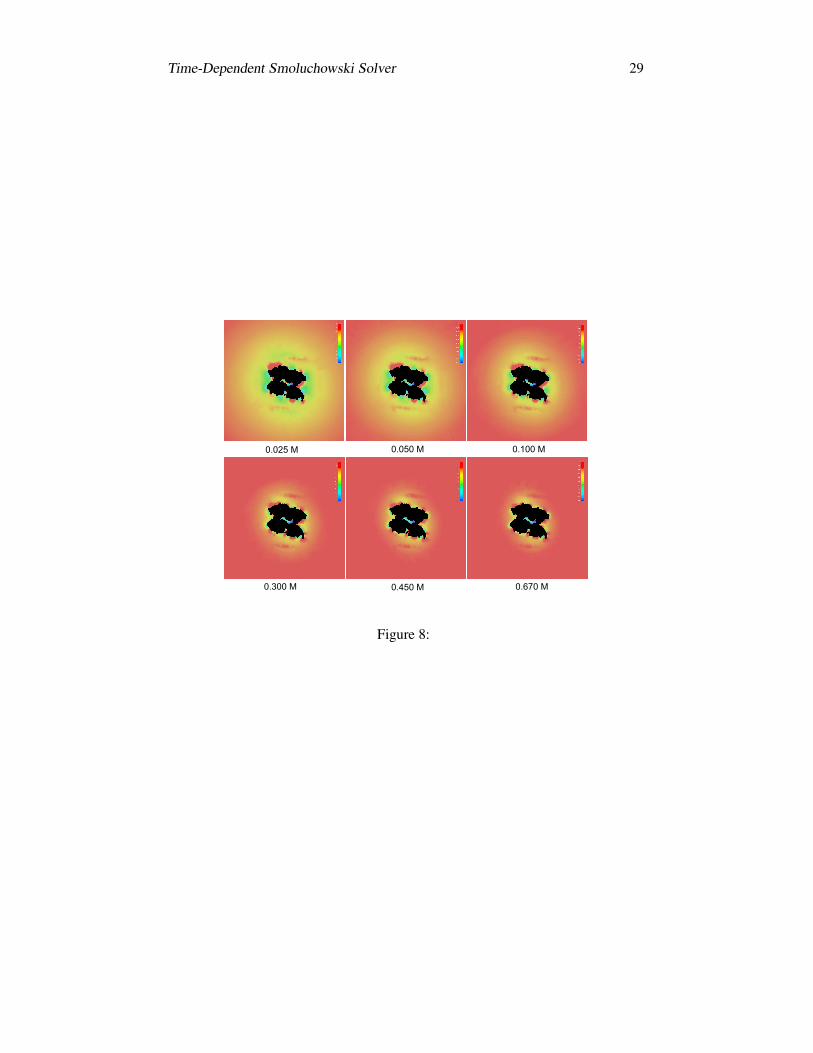
Similarly, we tested the final steady-state concentration distribution in the dif-fusion domain under various ionic strength conditions for the AChE tetramers.For example, Fig. 8 illustrates the different concentration profiles at 0.025, 0.050,0.100, 0.300, 0.450, 0.670M ionic strength solutions for structure 1C2O. Compar-ing with the monomer case, the ACh-like ligand concentration around the 1C2Omolecule is much lower when the ionic strength is small, due to the stronger elec-trostatic attraction between the ligands and the tetramer molecule. While the ionicstrength becomes higher, the electrostatic effect on the steady-state concentrationdistribution turns out to be weaker.

We also obtained the time-dependent rate constant per active site for the struc-ture 1C2B, in which all the four gorges are nearly completely accessible to thesolvent (Fig. 7). The profiles of kon(t) of AS3 and AS4 are almost the same,while the value of the final steady state for AS1 or AS2 is a little smaller, butstill above 1.10 × 1011M−1min−1. The sum of the four active sites is 5.28 ×1011M−1min−1, whereas the total steady-state kon in structure 1C2O is 4.92 ×1011M−1min−1. It must be noted that the steady-state kon in the mAChE monomeris 1.97 × 1011M−1min−1 at 0.150 M ionic strength. Therefore, the average re-action rate per active site for the tetramer is around 64% that of the monomer,which is close to the result of the previous SSSE studies (20). The four active sitesshow similar kinetic profiles, and reach the steady states at nearly the same time.Meanwhile, the time-dependent rate constant per active site in the structure INTappears more like that in the structure 1C2B, although the difference between AS1


amd AS3 is still similar with that in the structure 1C2O. Additionally, our time-dependent SMOL solver can show the detailed diffusion process. For the 1C2Ocase, Fig. 9 describes the ligand concentration distribution in the problem domain.The red represents high concentration areas, while the blue represents the low con-centration areas.

ConclusionsIn this study, we describe new continuum-based methods for studying diffusion inbiomolecular systems. Specifically, we present the time-dependent SMOL soft-ware package, a finite element-based set of tools for solving the TDSE to calculateligand binding rate constants for large biomolecules under pre-steady-state andsteady-state conditions. The main improvement from the previous SMOL solver(9, 10) can be addressed as below: first, the new solver has removed the drift term(Eq. 2) which is discontinuous for ∇W , as well as the asymmetry (47). Theoreti-cally, the new SMOL solver can utilize the conjugate gradient (CG) method whichis a direct method for symmetric and positive definite linear systems, while the oldsolver can only solve SSSE with the Bi-conjugate gradient (BCG) method. Com-paring with the new solver, BCG is slower and harder to converge. Therefore, ournew SMOL solver can solve both steady-state and time-dependent problems muchmore efficiently and stably than the old version.

With the new code, we solved the time-dependent diffusion in the analyti-cal case of a reactive sphere, mAChE monomer and tetramer cases. Comparingwith previous steady state studies, our research extends the study into the non-equilibrium diffusion dynamics and obtained very consistent results. Moreover,the calculated rates of the mAChE monomer were compared with experimentaldata (27) and show very good agreement with experiment while requiring substan-tially less computational effort than existing particle-based Brownian dynamicsmethods. Additionally, the value of kon(t) seems to be underestimated with thecoarser meshes, which is consistent with previous observations (10). Similarly, thekon values in mAChE tetramers should increase if we refine the original mesh. Inthe previous study (20) and this one, we have found the activity of one subunit ina mAChE tetramer equals around 60% ∼ 70% that of a free monomer. With theappropriate meshes, we would expect to obtain an activity closer to that in the freemonomer and the catalytic activity might not be too affected by subunit associationas suggested in the experiment (48).

Additionally, we describe new adaptive meshing methods developed to dis-cretize biomolecular systems into finite element meshes which respect the geom-etry of the biomolecule. Although not presented in this study, it is important to


note that the new meshing methods could be useful in a variety of biological simu-lations including computational studies of biomolecular electrophoresis (49), elas-ticity (42, 43), and electrostatics (35, 36, 50, 51).

Finally, this research lays the groundwork for the integration of molecular-scaleinformation into simulations of cellular-scale systems such as the neuromuscularjunction (6, 11, 52). In particular, this new finite element framework should facili-tate the incorporation of other continuum mechanics phenomena into biomolecularsimulations. The ultimate goal of this work is to develop scalable methods and the-ories that will allow researchers to begin to study biological dynamics in a cellularcontext efficiently and robustly.

1 ACKNOWLEDGEMENTSY.H.C. thank David Minh for proofreading, and Ben-Zhuo Lu for helpful discus-sions. This work has been supported in part by grants from the NSF and NIH.Additional support has been provided by NBCR, CTBP, HHMI, and the W. M.Keck Foundation.

References1. Ermak, D. L., and J. A. McCammon. 1978. Brownian dynamics with hydro-

dynamic interactions. J. Chem. Phys. 69:1352–1360.

2. Northrup, S. H., S. A. Allison, and J. A. McCammon. 1984. Brownian dynam-ics simulation of diffusion-influenced bimolecular reactions. J. Chem. Phys.80:1517–1526.

3. Agmon, N., and A. L. Edelstein. 1997. Collective binding properties of recep-tor arrays. Biophys. J. 72:1582–1594.

4. Gabdoulline, R. R., and R. C. Wade. 1998. Brownian dynamics simulation ofprotein-protein diffusional encounter. Methods 14:329–341.

5. Stiles, J. R., and T. M. Bartol. 2000. Monte Carlo methods for simulating real-istic synaptic microphysiology using MCell. In Computational Neuroscience:Realistic Modeling for Experimentalists, E. D. Schutter, editor. CRC Press,Inc., New York, 87–127.

6. Smart, J. L., and J. A. McCammon. 1998. Analysis of synaptic transmission inthe neuromuscular junction using a continuum finite element model. Biophys.J. 75:1679–1688.


7. Kurnikova, M. G., R. D. Coalson, P. Graf, and A. Nitzan. 1999. A latticerelaxation algorithm for three-dimensional poisson-nernst-planck theory withapplication to ion transport through the gramicidin a channel. Biophys. J.76:642–656.

8. Schuss, Z., B. Nadler, and R. S. Eisenberg. 2001. Derivation of poisson andnernst-planck equations in a bath and channel from a molecular model. Phys.Rev. E 6403.

9. Song, Y. H., Y. J. Zhang, C. L. Bajaj, and N. A. Baker. 2004. Continuumdiffusion reaction rate calculations of wild-type and mutant mouse acetyl-cholinesterase: adaptive finite element analysis. Biophys. J. 87:1558–1566.

10. Song, Y. H., Y. J. Zhang, T. Y. Shen, C. L. Bajaj, A. McCammon, and N. A.Baker. 2004. Finite element solution of the steady-state smoluchowski equa-tion for rate constant calculations. Biophys. J. 86:2017–2029.

11. Tai, K. S., S. D. Bond, H. R. Macmillan, N. A. Baker, M. J. Holst, and J. A.McCammon. 2003. Finite element simulations of acetylcholine diffusion inneuromuscular junctions. Biophys. J. 84:2234–2241.

12. Berry, H. 2002. Monte carlo simulations of enzyme reactions in two dimen-sions: fractal kinetics and spatial segregation. Biophys. J. 83:1891–1901.

13. Genest, D. 1989. A monte-carlo simulation study of the influence of internalmotions on the molecular-conformation deduced from two-dimensional nmrexperiments. Biopolymers 28:1903–1911.

14. Saxton, M. J. 1992. Lateral diffusion and aggregation - a monte-carlo study.Biophys. J. 61:119–128.

15. McCammon, J. A. 1987. Computer-aided molecular design. Science 238:486–491.

16. Northrup, S. H., J. O. Boles, and J. C. L. Reynolds. 1988. Brownian dynamicsof cytochrome-c and cytochrome-c peroxidase association. Science 241:67–70.

17. Wade, R. C., M. E. Davis, B. A. Luty, J. D. Madura, and J. A. Mccammon.1993. Gating of the active-site of triose phosphate isomerase - brownian dy-namics simulations of flexible peptide loops in the enzyme. Biophys. J. 64:9–15.


18. Eastman, P., and S. Doniach. 1998. Multiple time step diffusive langevin dy-namics for proteins. Proteins 30:215–227.

19. Yeomans-Reyna, L., and M. Medina-Noyola. 2001. Self-consistent general-ized langevin equation for colloid dynamics. Phys Rev E Stat Nonlin SoftMatter Phys. 64:066114.

20. Zhang, D. Q., J. Suen, Y. J. Zhang, Y. H. Song, Z. Radic, P. Taylor, M. J.Holst, C. Bajaj, N. A. Baker, and J. A. McCammon. 2005. Tetrameric mouseacetylcholinesterase: continuum diffusion rate calculations by solving thesteady-state Smoluchowski equation using finite element methods. Biophys. J.88:1659–1665.

21. Wang, J. 2006. Diffusion and single molecule dynamics on biomolecular in-terface binding energy landscape. Chem. Phys. Lett. 418:544–548.

22. Berg, J. M., J. L. Tymoczko, and L. Stryer. 1995. In Biochemistry. W. H.Freeman & Co., New York, NY.

23. Bazelyansky, M., E. Robey, and J. F. Kirsch. 1986. Fractional diffusion-limited component of reactions catalyzed by acetylcholinesterase. Biochem-istry 25:125–130.

24. Berman, H. A., K. Leonard, and M. W. Nowak. 1991. In Cholinesterases:Structure, Function, Mechanism, Genetics and Cell Biology. American Chem-ical Society, Washington, DC. J. Massoulie, editor.

25. Nolte, H. J., T. L. Rosenberry, and E. Neumann. 1980. Effective chargeon acetylcholinesterase active-sites determined from the ionic-strength de-pendence of association rate constants with cationic ligands. Biochemistry19:3705–3711.

26. Bourne, Y., P. Taylor, and P. Marchot. 1995. Acetylcholinesterase inhibitionby fasciculin - crystal-structure of the complex. Cell 83:503–512.

27. Radic, Z., D. M. Quinn, J. A. McCammon, and P. Taylor. 1997. Electrostaticinfluence on the kinetics of ligand binding to acetylcholinesterase - distinctionsbetween active center ligands and fasciculin. J. Biol. Chem. 272:23265–23277.

28. Velsor, L. W., C. A. Ballinger, J. Patel, and E. M. Postlethwait. 2003. Influ-ence of epithelial lining fluid lipids on no-2-induced membrane oxidation andnitration. Free Radic. Biol. Med. 34:720–733.


29. Tan, R. C., T. N. Truong, J. A. McCammon, and J. L. Sussman. 1993. Acetyl-cholinesterase - electrostatic steering increases the rate of ligand-binding. Bio-chemistry 32:401–403.

30. Tara, S., A. H. Elcock, J. M. Briggs, Z. Radic, P. Taylor, and J. A. McCam-mon. 1998. Rapid binding of a cationic active site inhibitor to wild type andmutant mouse acetylcholinesterase: brownian dynamics simulation includingdiffusion in the active site gorge. Biopolymers 46:465–474.

31. Zhou, H. X. 1990. On the calculation of diffusive reaction-rates using brown-ian dynamics simulations. J. Chem. Phys. 92:3092–3095.

32. Zhou, H. X., S. T. Wlodek, and J. A. McCammon. 1998. Conformation gat-ing as a mechanism for enzyme specificity. Proc. Natl. Acad. Sci. U. S. A.95:9280–9283.

33. Zhou, H. X., J. M. Briggs, S. Tara, and J. A. McCammon. 1998. Correla-tion between rate of enzyme-substrate diffusional encounter and average boltz-mann factor around active site. Biopolymers 45:355–360.

34. Axelsson, O., and V. A. Barker. 2001. In Finite Element Solution of BoundaryValue Problems. Theory and Computation. Society for Industrial and AppliedMathematics, Philadelphia, PA.

35. Holst, M., N. Baker, and F. Wang. 2000. Adaptive multilevel finite elementsolution of the poisson-boltzmann equation i. algorithms and examples. J.Comput. Chem. 21:1319–1342.

36. Baker, N., M. Holst, and F. Wang. 2000. Adaptive multilevel finite elementsolution of the poisson-boltzmann equation ii. refinement at solvent-accessiblesurfaces in biomolecular systems. J. Comput. Chem. 21:1343–1352.

37. Holst, M. 2001. Adaptive numerical treatment of elliptic systems on mani-folds. Adv. Comput. Math. 15:139–191.

38. Braess, D. 1997. In Finite Elements: Theory, Fast Solvers, and Applicationsin Solid Mechanics. Cambridge University Press, New York, NY.

39. Lu, B. Z., X. L. Cheng, T. J. Hou, and J. A. McCammon. 2005. Calculationof the maxwell stress tensor and the poisson-boltzmann force on a solvatedmolecular surface using hypersingular boundary integrals. J. Chem. Phys. 123.

40. Lu, B. Z., D. Q. Zhang, and J. A. McCammon. 2005. Computation of electro-static forces between solvated molecules determined by the poisson-boltzmannequation using a boundary element method. J. Chem. Phys. 122.


41. Humphrey, W., A. Dalke, and K. Schulten. 1996. Vmd: visual moleculardynamics. J. Mol. Graph. 14:33–38.

42. Zhang, Y. J., C. L. Bajaj, and B. S. Sohn. 2003. Adaptive and quality 3-dmeshing from imaging data. In Proc. 8th ACM Symposium on Solid Modelingand Applications. ACM Press, Seattle, WA., 286291.

43. Zhang, Y. J., C. L. Bajaj, and B. S. Sohn. 2004. 3d finite element meshingfrom imaging data. the special issue of Computer Methods in Applied Mechan-ics and Engineering (CMAME) on Unstructured Mesh generation 194:5083–5106.

44. Zhang, Y. J., G. L. Xu, and C. Bajaj. 2006. Quality meshing of implicit solva-tion models of biomolecular structures. Comput. Aided Geom. Des. 23:510–530.

45. Krissinel, E. B., and N. Agmon. 1996. Spherical symmetric diffusion problem.J. Comput. Chem. 17:1085–1098.

46. Quinn, D. M., J. Seravalli, H. K. Nair, R. Medhekar, B. Husseini, Z. Radic,D. C. Vellom, N. Pickering, and P. Taylor. 1995. The function of electrostaticsin acetylcholinesterase catalysis. In Enzymes of the Cholinesterase Family.Plenum Publishing, New York, NY, 203207. D. M. Quinn, A. S. Balasubra-manian, B. P. Doctor, and P. Taylor, editors.

47. Holst, M., and S. Vandewalle. 1997. Schwarz methods: to symmetrize or notto symmetrize. SIAM J. Numer. Anal. 34:699–722.

48. Saxena, A., R. S. Hur, C. Y. Luo, and B. P. Doctor. 2003. Natural monomericform of fetal bovine serum acetylcholinesterase lacks the c-terminal tetramer-ization domain. Biochemistry 42:15292–15299.

49. Allison, S. A. 2001. Boundary element modeling of biomolecular transport.Biophys. Chem. 93:197–213.

50. Cortis, C. M., and R. A. Friesner. 1997. Numerical solution of the poisson-boltzmann equation using tetrahedral finite-element meshes. J. Comput. Chem.18:1591–1608.

51. Cortis, C. M., and R. A. Friesner. 1997. An automatic three-dimensional fi-nite element mesh generation system for the poisson-boltzmann equation. J.Comput. Chem. 18:1570–1590.


52. Cheng, Y. H., J. K. Suen, Z. Radic, S. D. Bond, M. J. Holst, and J. A. McCm-mon. 2007. Continuum simulations of acetylcholine diffusion with reaction-determined boundaries in neuromuscular junction models. Biophys. Chem.accepted.


Table 1: SSSE reaction rate and TDSE final reaction rate constants as a function ofionic strength

ionic strength (M) 0.000 0.025 0.100 0.300 0.600SSSE results kon(1011M−1min−1) 9.562 3.681 2.304 1.572 1.302TDSE final results kon(1011M−1min−1) 9.535 3.673 2.298 1.569 1.298


Figure LegendsFigure 1.

Illustration of the discretized problem domain for the spherical analytical test. Thegreen represents the outer boundary, in which the ligand concentration is kept as aconstant.

Figure 2.

Time evolution of the 2D concentration distribution contour in the problem domain.(a) our SMOL solution;(b) spherical analytical solution.

Figure 3.

kon(t) values in time-dependent ACh diffusion under the various ionic strength con-ditions.

Figure 4.

2D ligand concentration distribution contour around mAChE at the steady stateunder various ionic strengths. The red color represents high concentration area,while the blue represents low concentration area.

Figure 6.

The comparison of kon values in time-dependent ACh diffusion between the origi-nal and refined meshes.

Figure 7.

The dependency of kon(t) values on the simulation time for the structures 1C2O,INT and 1C2B: (a) 0.150 M ionic strength and +1.0e ligand;(b) neutral ACh-likeligand.

Figure 8.

Steady-state ligand concentration distribution under 6 different ionic strength con-ditions for structure 1C2O.


Figure 9.

ligand concentration distribution in the diffusion domain during the simulation timefor structure 1C2O.


Figure 1:


Figure 2:


0 5 10 15 20Time, µs

0

2e+11

4e+11

6e+11

8e+11

1e+12

k on, M

-1m

in-1

Ionic Strength = 0.000 MIonic Strength = 0.050 MIonic Strength = 0.100 MIonic Strength = 0.150 MIonic Strength = 0.200 MIonic Strength = 0.250 MIonic Strength = 0.300 MIonic Strength = 0.450 MIonic Strength = 0.600 MIonic Strength = 0.670 M

Figure 3:


Figure 4:


Figure 5:


0 5 10 15 20Time, µs

0

5e+10

1e+11

1.5e+11

2e+11

2.5e+11

3e+11

k on(t)

, M-1

min

-1

Refined MeshOriginal Mesh

Figure 6:


0

5e+10

1e+11

1.5e+11

2e+11

k on, M

-1m

in-1

AS1AS2AS3AS4

0

5e+10

1e+11

1.5e+11

2e+11

0

5e+10

1e+11

1.5e+11

2e+11

0 50 100 1500

2e+10

4e+10

6e+10

8e+10

0 50 100 150Time, µs

0

2e+10

4e+10

6e+10

8e+10

0 50 100 1500

2e+10

4e+10

6e+10

8e+10

(a)

(b)

(a) (a)

(b) (b)

1C2O INT 1C2B

Figure 7:


Figure 8:


Figure 9:

Finite Element Analysis of the Time-Dependent …ccom.ucsd.edu/~mholst/pubs/dist/CSZB06.pdf ·...

Documents

Transcript of Finite Element Analysis of the Time-Dependent …ccom.ucsd.edu/~mholst/pubs/dist/CSZB06.pdf ·...