Finite Element Analysis of Composite Laminates - Aaltomath.aalto.fi/~jkonno/nscm20.pdf · Finite...
51
Finite Element Analysis of Composite Laminates 20th Nordic Seminar on Computational Mechanics Juho Könnö [email protected] Helsinki University of Technology Institute of Mathematics
Transcript of Finite Element Analysis of Composite Laminates - Aaltomath.aalto.fi/~jkonno/nscm20.pdf · Finite...

Finite Element Analysis ofComposite Laminates20th Nordic Seminar on Computational Mechanics
Juho Könnö
Helsinki University of Technology
Institute of Mathematics

Outline of the talk
Mathematical model using the Reissner-Mindlinkinematic assumptions
20th Nordic Seminar on Computational Mechanics – p.1

Outline of the talk
Mathematical model using the Reissner-Mindlinkinematic assumptions
Finite element formulation
20th Nordic Seminar on Computational Mechanics – p.1

Outline of the talk
Mathematical model using the Reissner-Mindlinkinematic assumptions
Finite element formulation
The mixed interpolation technique for theReissner-Mindlin model
20th Nordic Seminar on Computational Mechanics – p.1

Outline of the talk
Mathematical model using the Reissner-Mindlinkinematic assumptions
Finite element formulation
The mixed interpolation technique for theReissner-Mindlin model
The paper cockling problem
20th Nordic Seminar on Computational Mechanics – p.1

A typical configuration
z
zk+1
zk−1
g f
Ω
z
y
x
zk
20th Nordic Seminar on Computational Mechanics – p.2

Mathematical model
Basic idea:
Use Reissner-Mindlin kinematic assumptions
Take into account the in-plane displacement
20th Nordic Seminar on Computational Mechanics – p.3

Mathematical model
Basic idea:
Use Reissner-Mindlin kinematic assumptions
Take into account the in-plane displacement
Result:
Coupled problem consisting ofplane elasticity problemReissner-Mindlin plate problem
20th Nordic Seminar on Computational Mechanics – p.3

Constitutive relations
Use classical lamination theory
20th Nordic Seminar on Computational Mechanics – p.4

Constitutive relations
Use classical lamination theory
From the constitutive tensors of individual layers wederive:
A - the plane elasticity tensorD - the bending deformation tensorB - the coupling tensorA∗ - the shear deformation tensor
20th Nordic Seminar on Computational Mechanics – p.4

Constitutive relations
Use classical lamination theory
From the constitutive tensors of individual layers wederive:
A - the plane elasticity tensorD - the bending deformation tensorB - the coupling tensorA∗ - the shear deformation tensor
Each tensor is a weighted sum of the originalconstitutive tensors ⇒ easy to compute
20th Nordic Seminar on Computational Mechanics – p.4

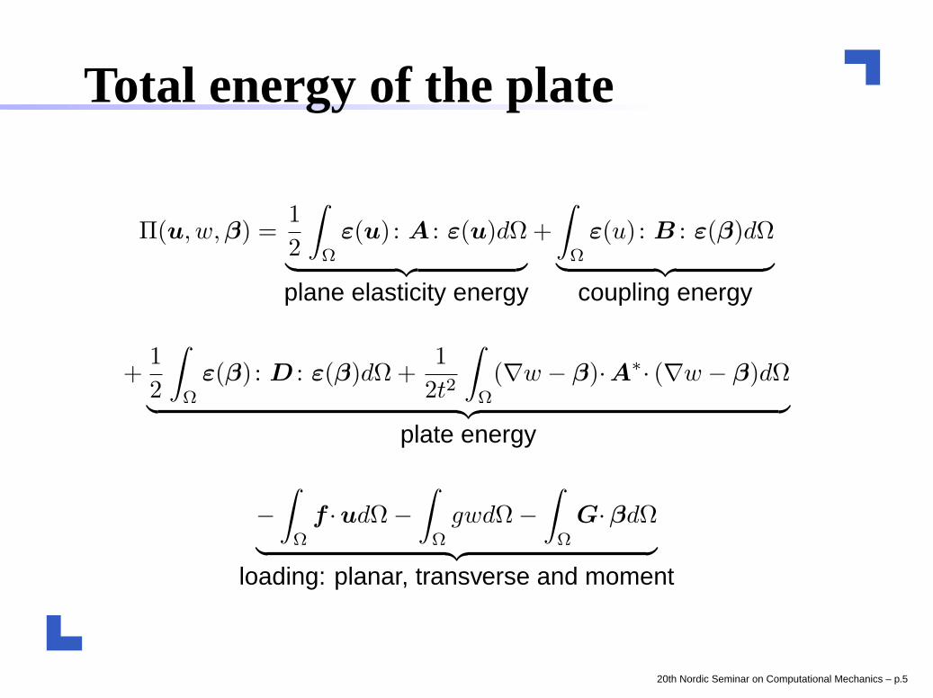
Total energy of the plate
Π(u, w,β) =1
2
∫
Ω
ε(u) : A : ε(u)dΩ
︸ ︷︷ ︸
plane elasticity energy
+
∫
Ω
ε(u) : B : ε(β)dΩ
︸ ︷︷ ︸
coupling energy
20th Nordic Seminar on Computational Mechanics – p.5

Total energy of the plate
Π(u, w,β) =1
2
∫
Ω
ε(u) : A : ε(u)dΩ
︸ ︷︷ ︸
plane elasticity energy
+
∫
Ω
ε(u) : B : ε(β)dΩ
︸ ︷︷ ︸
coupling energy
+1
2
∫
Ω
ε(β) : D : ε(β)dΩ +1
2t2
∫
Ω
(∇w − β)·A∗· (∇w − β)dΩ
︸ ︷︷ ︸
plate energy
20th Nordic Seminar on Computational Mechanics – p.5
Total energy of the plate
Π(u, w,β) =1
2
∫
Ω
ε(u) : A : ε(u)dΩ
︸ ︷︷ ︸
plane elasticity energy
+
∫
Ω
ε(u) : B : ε(β)dΩ
︸ ︷︷ ︸
coupling energy
+1
2
∫
Ω
ε(β) : D : ε(β)dΩ +1
2t2
∫
Ω
(∇w − β)·A∗· (∇w − β)dΩ
︸ ︷︷ ︸
plate energy
−
∫
Ω
f ·udΩ −
∫
Ω
gwdΩ −
∫
Ω
G·βdΩ
︸ ︷︷ ︸
loading: planar, transverse and moment
20th Nordic Seminar on Computational Mechanics – p.5
Weak formulation
Minimize the energy with respect to the variablesu, w,β
20th Nordic Seminar on Computational Mechanics – p.6

Weak formulation
Minimize the energy with respect to the variablesu, w,β
Two coupled equations: plate problem and planeelasticity problem
20th Nordic Seminar on Computational Mechanics – p.6

Weak formulation
Minimize the energy with respect to the variablesu, w,β
Two coupled equations: plate problem and planeelasticity problem
Coupling is of elliptic nature
20th Nordic Seminar on Computational Mechanics – p.6

Displacement formulation
In displacement formulation the weak problem isProblem 1. Find (u, w,β) ∈ U × W × V such that ∀(v, ν,η) ∈ U × W × V
it holds
(A : ε(u), ε(v)) + (B : ε(v), ε(β)) = (f , v),
(B : ε(u), ε(η)) + (D : ε(β), ε(η))
+t−2(A∗· (∇w − β), (∇ν − η)) = (g, ν) + (G, η)
20th Nordic Seminar on Computational Mechanics – p.7

Displacement formulation
In displacement formulation the weak problem isProblem 1. Find (u, w,β) ∈ U × W × V such that ∀(v, ν,η) ∈ U × W × V
it holds
(A : ε(u), ε(v)) + (B : ε(v), ε(β)) = (f , v),
(B : ε(u), ε(η)) + (D : ε(β), ε(η))
+t−2(A∗· (∇w − β), (∇ν − η)) = (g, ν) + (G, η)
We can also treat the shear force q = t−2A∗· (∇w − β)
as an independent unknown
20th Nordic Seminar on Computational Mechanics – p.7

Mixed formulation
The mixed formulation with the shear force as anindependent unknown isProblem 2. Find (u, w,β, q) ∈ U × W × V × Γ such that
∀(v, ν,η, s) ∈ U × W × V × Γ it holds
(A : ε(u), ε(v)) + (B : ε(v), ε(β)) = (f,v),
(B : ε(u), ε(η)) + (D : ε(β), ε(η)) + (q,∇ν − η) = (g, ν) + (G, η),
(t2A∗−1q, s) + ((∇w − β), s) = 0,
where U × W × V × Γ ⊂ [H1(Ω)]2 × H1(Ω) × [H1(Ω)]2 × [L2(Ω)]2.
20th Nordic Seminar on Computational Mechanics – p.8

Mixed-interpolated finite elements
Solving Problem 1 or 2 with ”normal” basis functionsleads to locking
20th Nordic Seminar on Computational Mechanics – p.9

Mixed-interpolated finite elements
Solving Problem 1 or 2 with ”normal” basis functionsleads to locking
Solution: introduce a reduction operator on thediscrete spaces Rh : Vh → Γh and replace(∇w − β) → Rh(∇w − β)
20th Nordic Seminar on Computational Mechanics – p.9

Mixed-interpolated finite elements
Solving Problem 1 or 2 with ”normal” basis functionsleads to locking
Solution: introduce a reduction operator on thediscrete spaces Rh : Vh → Γh and replace(∇w − β) → Rh(∇w − β)
Does not completely solve the locking problem, wefurther need
mesh-dependent stabilization
20th Nordic Seminar on Computational Mechanics – p.9

Mixed-interpolated finite elements
Solving Problem 1 or 2 with ”normal” basis functionsleads to locking
Solution: introduce a reduction operator on thediscrete spaces Rh : Vh → Γh and replace(∇w − β) → Rh(∇w − β)
Does not completely solve the locking problem, wefurther need
mesh-dependent stabilizationunequal interpolation
20th Nordic Seminar on Computational Mechanics – p.9

Main idea of the error analysis
Error analysis with the mixed formulation as astarting point
20th Nordic Seminar on Computational Mechanics – p.10

Main idea of the error analysis
Error analysis with the mixed formulation as astarting point
Problems to deal with
20th Nordic Seminar on Computational Mechanics – p.10
Main idea of the error analysis
Error analysis with the mixed formulation as astarting point
Problems to deal withStability issues
20th Nordic Seminar on Computational Mechanics – p.10

Main idea of the error analysis
Error analysis with the mixed formulation as astarting point
Problems to deal withStability issuesConsistency error
20th Nordic Seminar on Computational Mechanics – p.10

Main idea of the error analysis
Error analysis with the mixed formulation as astarting point
Problems to deal withStability issuesConsistency error
Restriction to a quasiuniform mesh needed
20th Nordic Seminar on Computational Mechanics – p.10

Main idea of the error analysis
Error analysis with the mixed formulation as astarting point
Problems to deal withStability issuesConsistency error
Restriction to a quasiuniform mesh needed
Adding the plane elasticity problem to the estimate ⇒use ellipticity
20th Nordic Seminar on Computational Mechanics – p.10

Main a priori result
We get the following error estimate
‖β − βh‖1 + ‖w − wh‖1 + t‖q − qh‖0 + ‖q − qh‖−1 + ‖u − uh‖1 ≤
Chki (‖g‖s−2,Ωi
+t‖g‖s−1,Ωi+‖F ‖s−1,Ωi
)+hb(‖g‖−1+t‖g‖0+‖F ‖0),
where F is defined as
‖F ‖2
s = ‖f‖2
s + ‖G‖2
s.
20th Nordic Seminar on Computational Mechanics – p.11

Main a priori result
We get the following error estimate
‖β − βh‖1 + ‖w − wh‖1 + t‖q − qh‖0 + ‖q − qh‖−1 + ‖u − uh‖1 ≤
Chki (‖g‖s−2,Ωi
+t‖g‖s−1,Ωi+‖F ‖s−1,Ωi
)+hb(‖g‖−1+t‖g‖0+‖F ‖0),
where F is defined as
‖F ‖2
s = ‖f‖2
s + ‖G‖2
s.
So, what’s the application then?
20th Nordic Seminar on Computational Mechanics – p.11

The paper cockling problem
Cockling deals with small-scale deformations, mostlydue to moisture changes
20th Nordic Seminar on Computational Mechanics – p.12
The paper cockling problem
Cockling deals with small-scale deformations, mostlydue to moisture changes
In general, paper is a difficult material to model
20th Nordic Seminar on Computational Mechanics – p.12

The paper cockling problem
Cockling deals with small-scale deformations, mostlydue to moisture changes
In general, paper is a difficult material to modelArbritrary fiber orientation
20th Nordic Seminar on Computational Mechanics – p.12

The paper cockling problem
Cockling deals with small-scale deformations, mostlydue to moisture changes
In general, paper is a difficult material to modelArbritrary fiber orientationHeterogeneous
20th Nordic Seminar on Computational Mechanics – p.12

The paper cockling problem
Cockling deals with small-scale deformations, mostlydue to moisture changes
In general, paper is a difficult material to modelArbritrary fiber orientationHeterogeneous
Simplification: divide the sheet into layers
20th Nordic Seminar on Computational Mechanics – p.12
The paper cockling problem
Cockling deals with small-scale deformations, mostlydue to moisture changes
In general, paper is a difficult material to modelArbritrary fiber orientationHeterogeneous
Simplification: divide the sheet into layersFiber orientation varies ⇒ form constitutive tensorin each data block
20th Nordic Seminar on Computational Mechanics – p.12

The paper cockling problem
Cockling deals with small-scale deformations, mostlydue to moisture changes
In general, paper is a difficult material to modelArbritrary fiber orientationHeterogeneous
Simplification: divide the sheet into layersFiber orientation varies ⇒ form constitutive tensorin each data blockUse classical lamination theory blockwise
20th Nordic Seminar on Computational Mechanics – p.12

Material model
Only global parameters are measurable
20th Nordic Seminar on Computational Mechanics – p.13

Material model
Only global parameters are measurable
Local structure defined by
20th Nordic Seminar on Computational Mechanics – p.13

Material model
Only global parameters are measurable
Local structure defined byOrientation angle
20th Nordic Seminar on Computational Mechanics – p.13
Material model
Only global parameters are measurable
Local structure defined byOrientation angleLevel of anisotropy
20th Nordic Seminar on Computational Mechanics – p.13

Material model
Only global parameters are measurable
Local structure defined byOrientation angleLevel of anisotropy
Combining the above two we obtain the localconstitutive relation
20th Nordic Seminar on Computational Mechanics – p.13

Material model
Only global parameters are measurable
Local structure defined byOrientation angleLevel of anisotropy
Combining the above two we obtain the localconstitutive relation
Empirical models used for the moisture dependenceof global parameters
20th Nordic Seminar on Computational Mechanics – p.13

Problems in modelling
Choice of proper boundary conditions
20th Nordic Seminar on Computational Mechanics – p.14

Problems in modelling
Choice of proper boundary conditions
Computational time
20th Nordic Seminar on Computational Mechanics – p.14
Problems in modelling
Choice of proper boundary conditions
Computational time
Need for large deformations theory?
20th Nordic Seminar on Computational Mechanics – p.14

Effect of the boundary conditions
Figure 1: Simply supported, free plane Figure 2: Simply supported, fixed plane
20th Nordic Seminar on Computational Mechanics – p.15

Thank you for your attention
20th Nordic Seminar on Computational Mechanics – p.16