Finite Element Analysis - Al-Ameen Engineering College€¦ · differential equations in...
155
A Course Material on Finite Element Analysis By ASSISTANT PROFESSOR DEPARTMENT OF MECHANICAL ENGINEERING AL AMEEN ENGINEERING COLLEGE ERODE – 638 104 Mr. M.SURENDRAN ME., (Ph.D) R.GOPINATH ME
-
Upload
trinhthien -
Category
Documents
-
view
223 -
download
0
Transcript of Finite Element Analysis - Al-Ameen Engineering College€¦ · differential equations in...

A Course Material on
Finite Element Analysis
By
ASSISTANT PROFESSOR
DEPARTMENT OF MECHANICAL ENGINEERING
AL AMEEN ENGINEERING COLLEGE
ERODE – 638 104
Mr. M.SURENDRAN ME., (Ph.D) R.GOPINATH ME

QUALITY CERTIFICATE
This is to certify that the e-course material
Subject : Finite Element Analysis
Class : III Year Mechanical
being prepared by me and it meets the knowledge requirement of the university curriculum.
Signature of the Author
Designation: ASSISTANT PROFESSOR
SEAL
Subject Code : ME6603
Name: M.SURENDRAN M.E., (Ph.D)
Name: PROF. G.THANGAVEL M.E., M.B.A.,
Signature of HOD

CONTENTSS.NO TOPIC PAGE NO
UNIT-1 FINITE ELEMENT FORMULATION OF BOUNDARY VALUE PROBLEMS
1.1 INTRODUCTION 1
1.1.1 A Brief History of the FEM 1
1.1.2General Methods of the Finite Element Analysis 1
1.1.3General Steps of the Finite Element Analysis 1
1.1.4 Objectives of This FEM 2
1.1.5 Applications of FEM in Engineering 2
1.2 WEIGHTED RESIDUAL METHOD 2
1.3 THE GENERAL WEIGHTED RESIDUAL STATEMENT 5
1.4 WEAK FORMULATION OF THE WEIGHTED RESIDUAL 5
1.5 PIECE WISE CONTINUOUS TRIAL FUNCTION 6
1.6 EXAMPLES OF A BAR FINITE ELEMENT 8
1.6.1 Rigid Body 13
1.7 PRINCIPLE OF STATIONERY TOTAL POTENTIAL PSTP) 19
1.7.1 Potential energy in elastic bodies 19
1.7.2 Principle of Minimum Potential Energy 19
1.8 RAYLEIGH – RITZ METHOD (VARIATIONAL APPROACH) 24
1.9 ADVANTAGES OF FINITE ELEMENT METHOD 24
1.10 DISADVANTAGES OF FINITE ELEMENT METHOD 24
UNIT – 2 ONE DIMENSIONAL FINITE ELEMENT ANALYSIS
2.1 ONE DIMENSIONAL ELEMENTS 25
2.2 LINEAR STATIC ANALYSIS( BAR ELEMENT) 28
2.3 BEAM ELEMENT 28
2.4 1-D 2-NODED CUBIC BEAM ELEMENT MATRICES 33
2.5 DEVELOPMENT OF ELEMENT EQUATION 34

2.6 BEAM ELEMENT 42
2.6.1 ELEMENT MATRICES AND VECTORS 45
UNIT – 3 TWO DIMENSIONAL FINITE ELEMENT ANALYSIS
3.1 INTRODUCTION 54
3.2 THREE NODED LINEAR TRIANGULAR ELEMENT 54
3.3 FOUR NODED LINEAR RECTANGULAR ELEMENT 55
3.4TWO-VARIABLE 3-NODED LINEAR TRIANGULAR
ELEMENT56
3.5 STRAIN – STRESS RELATION 60
3.5.1 Plane stress conditions 61
3.5.2 Plane strain conditions 61
3.6GENERALIZED COORDINATES APPROACH TO NODEL
APPROXIMATIONS65
3.7 ISOPARAMETRIC ELEMENTS 66
3.8STRUCTURAL MECHANICS APPLICATIONS IN 2DIMENSIONS
71
UNIT – 4 DYNAMIC ANALYSIS USING ELEMENT METHOD
4.1 INTRODUCTION 88
4.1.1 Fundamentals of Vibration 88
4.1.2 Causes of Vibrations 88
4.1.3 Types of Vibrations 88
4.2 EQUATION OF MOTION 89
4.3 CONSISTENT MASS MATRICES 94
4.3.1 Single DOF System 94
4.3.2.Multiple DOF System 98
4.4 VECTOR ITERATION METHODS 99
4.5 MODELLING OF DAMPING 102
4.5.1 Proportional Damping (Rayleigh Damping) 102
4.5.2 Frequency Response Analysis 105

4.6 TRANSIENT RESPONSE ANALYSIS 106
4.6.1Cautions in Dynamic Analysis 107
UNIT -5 APPLICATIONS IN HEAT TRANSFER &FLUID MECHANICS
5.1 ONE DIMENSIONAL HEAT TRANSFER ELEMENT 111
5.1.1Strong Form for Heat Conduction in One Dimension
with Arbitrary Boundary Conditions111
5.1.2Weak Form for Heat Conduction in One Dimension
with Arbitrary Boundary Conditions112
5.2 APPLICATION TO HEAT TRANSFER 2-DIMENTIONAL 112
5.2.1Strong Form for Two-Point Boundary Value Problems 112
5.2.2Two-Point Boundary Value Problem With
Generalized Boundary Conditions112
5.2.3 Weak Form for Two-Point Boundary Value Problems 114
5.3 SCALE VARIABLE PROBLEM IN 2 DIMENSIONS 114
5.4 2 DIMENTIONAL FLUID MECHANICS 117
QUESTION BANK 120
TEXT BOOKS:
1. P.Seshu, “Text Book of Finite Element Analysis”, Prentice-Hall of India Pvt. Ltd. NewDelhi, 2007.
2. J.N.Reddy, “An Introduction to the Finite Element Method”, McGraw-Hill InternationalEditions(Engineering Mechanics Series), 1993.
3. Cook,Robert.D., Plesha,Michael.E & Witt,Robert.J. “Concepts and Applications ofFinite Element Analysis”,Wiley Student Edition, 2004.
4. Chandrupatla & Belagundu, “Introduction to Finite Elements in Engineering”, 3rd
Edition, Prentice-Hall of India, Eastern Economy Editions.

1
UNIT II ONE DIMENSIONAL PROBLEM 9One Dimensional Second Order Equations – Discretization – Element types- Linear and Higher order Elements – Derivation of Shape functions and Stiffness matrices and force vectors- Assembly of Matrices – Solution of problems from solid mechanics and heat transfer. Longitudinal vibration frequencies and mode shapes. Fourth Order Beam Equation –Transverse deflections and Natural frequencies of beams.
UNIT III TWO DIMENSIONAL SCALAR VARIABLE PROBLEMS 9Second Order 2D Equations involving Scalar Variable Functions – Variational formulation –Finite Element formulation – Triangular elements – Shape functions and element matrices and vectors. Application to Field Problems – Thermal problems – Torsion of Non circular shafts –Quadrilateral elements – Higher Order Elements.
UNIT IV TWO DIMENSIONAL VECTOR VARIABLE PROBLEMS 9Equations of elasticity – Plane stress, plane strain and axisymmetric problems – Body forces and temperature effects – Stress calculations – Plate and shell elements.
REFERENCE BOOKS:1. Rao, S.S., “The Finite Element Method in Engineering”, 3rd Edition, Butterworth Heinemann, 20042. Logan, D.L., “A first course in Finite Element Method”, Thomson Asia Pvt. Ltd., 20023. Robert D. Cook, David S. Malkus, Michael E. Plesha, Robert J. Witt, “Concepts and Applications of Finite Element Analysis”, 4th Edition, Wiley Student Edition, 2002.4. Chandrupatla & Belagundu, “Introduction to Finite Elements in Engineering”, 3rd Edition, Prentice Hall College Div, 19905. Bhatti Asghar M, “Fundamental Finite Element Analysis and Applications”, John Wiley & Sons, 2005 (Indian Reprint 2013)
UNIT V ISOPARAMETRIC FORMULATION 9Natural co-ordinate systems – Isoparametric elements – Shape functions for iso parametric elements – One and two dimensions – Serendipity elements – Numerical integration and application to plane stress problems – Matrix solution techniques – Solutions Techniques to Dynamic problems – Introduction to Analysis Software.
OUTCOMES:Upon completion of this course, the students can able to understand different mathematical Techniques used in FEM analysis and use of them in Structural and thermal problem
TEXT BOOK:1. Reddy. J.N., “An Introduction to the Finite Element Method”, 3rd Edition, Tata McGraw-Hill, 20052. Seshu, P, “Text Book of Finite Element Analysis”, Prentice-Hall of India Pvt. Ltd., New Delhi, 2007.
OBJECTIVES:1. To introduce the concepts of Mathematical Modeling of Engineering Problems.2. To appreciate the use of FEM to a range of Engineering Problems
UNIT I INTRODUCTION 9Historical Background – Mathematical Modeling of field problems in Engineering – Governing Equations – Discrete and continuous models – Boundary, Initial and Eigen Value problems– Weighted Residual Methods – Variational Formulation of Boundary Value Problems – RitzTechnique – Basic concepts of the Finite Element Method.
ME6603 FINITE ELEMENT ANALYSIS L T P C 3 0 0 3

UNIT I
FINITE ELEMENT FORMULATION OF BOUNDARY VALUE PROBLEMS
1.1 INTRODUCTIONThe finite element method constitutes a general tool for the numerical solution of partial
differential equations in engineering and applied scienceThe finite element method (FEM), or finite element analysis (FEA), is based on the idea of
building a complicated object with simple blocks, or, dividing a complicated object into small andmanageable pieces. Application of this simple idea can be found everywhere in everyday life as well asin engineering.
Examples:Lego (kids’play) BuildingsApproximation of the area of a circle:
“Element” Si
i
R
Why Finite Element Method? Design analysis: hand calculations, experiments, and computer simulations FEM/FEA is the most widelyapplied computer simulation method in engineering Closelyintegrated with CAD/CAM applications
1.1.1 A Brief History of the FEM 1943 --- Courant (variational method) 1956 --- Turner, clough, martin and top(stiffness) 1960 --- Clough (finite element plan problems) 1970 --- Applications on mainframe computer 1980 --- Microcomputers, pre and post processors 1990 --- Analysis of large structural systems
1.1.2 General Methods of the Finite Element Analysis
1. Force Method – Internal forces are considered as the unknowns of the problem.
2. Displacement or stiffness method – Displacements of the nodes are considered as theunknowns of the problem.
1.1.3 General Steps of the Finite Element Analysis
Discretization of structure Numbering of Nodes and Elements Selection of Displacement function or interpolation function Define the material behavior by using Strain – Displacement and Stress – Strain
relationships
ME6603 Finite Element Analysis

Derivation of element stiffness matrix and equations Assemble the element equations to obtain the global or total equations Applying boundary conditions Solution for the unknown displacements computation of the element strains and stresses
from the nodal displacements Interpret the results (post processing).
1.1.4 Objectives of This FEM Understand the fundamental ideas of the FEM Know the behavior and usage of each type of elements covered in this course Be able to prepare a suitable FE model for given problems Can interpret and evaluate the quality of the results (know the physics of the problems) Be aware of the limitations of the FEM (don’t misuse the FEM - a numerical tool)
1.1.5 Applications of FEM in Engineering Mechanical/Aerospace/Civil/Automobile Engineering Structure analysis
(static/dynamic, linear/nonlinear) Thermal/fluid flows Electromagnetics Geomechanics Biomechanics
1.2 WEIGHTED RESIDUAL METHOD
It is a powerful approximate procedure applicable to several problems. For non – structural
problems, the method of weighted residuals becomes very useful. It has many types. The popular
four methods are,
1. Point collocation method,
Residuals are set to zero at n different locations Xi, and the weighting function wi
is denoted as (x - xi).
(x xi) R (x; a1, a2, a3… an) dx = 0
2. Subdomain collocation method
3. Least square method,
[R (x; a1, a2, a3… an)]2 dx = minimum.
4. Galerkin’smethod. wi = Ni (x)
Ni (x) [R (x; a1, a2, a3… an)]2 dx = 0, i = 1, 2, 3, …n.
Problem IFind the solution for the following differential equation.

EI −qo =0
The boundary conditions are u(0)=0, (0)=0,
(L)=0, (L)=0,
Given: The governing differential equation
EI −qo =0
Solution: assume a trial functionLet u(x) = a0+a1x+a2x
2+a3x3+a4x
4…..Apply 1st boundary conditionx=0, u(x)=00=a0+0a0=0
Apply 2nd boundary condition
x=0, =0
a1=0
Apply 3rd boundary condition
x=L, =0
a2=-[3a3L+6a4L2]
Apply 4th boundary condition
x=L, =0
a3=-4a4L
Substitute a0, a1, a2 and a3values in trial functionu(x)= 0+0-[3a3L+6a4L
2] -4a4Lu(x)= a4[6 L2x2-4 Lx3+ x4]
= a4[6 L2 (2x)-12 Lx2+ 4x3]
=24 a4
R= EI −qo =0
a4=
Substitute a4values in u(x)u(x) = [x4-4Lx3+6L2x2]
Result:Final solution u(x) = [x4-4Lx3+6L2x2]
Problem 2The differential equation of a physical phenomenon is given by

+ = 4, 0 ≤ ≤ 1The boundary conditions are: y(0)=0
y(1)=1Obtain one term approximate solution by using galerkin methodSolution:
Here the boundary conditions are not homogeneous so we assume a trial function as,y=a1x(x-1)+xfirst we have to verify whether the trial function satisfies the boundary condition or noty=a1x(x-1)+xwhen x=0, y=0
x=1, y=1Resuldual R:Y=a1x(x-1)+x=a1(x
2-x)+x
=a1(2x-1)+1= 2 1
Substitute value in given differential equation.
2a1+y=4xSubstitute y vlue
R=2a1+a1x(x-1)+x-4xIn galerkin’s method∫Substitute wi and R value in equationa1=0.83So one of the approximate solution is, y= 0.83x(x-1)+x
= 0.83x2-0.83x+xy=0.83 x2+0.17x
Problem 3Find the deflection at the center of a simply supported beam of span length l subjected to
uniform distributed load throughout its length as shown using (a) point collection method (b) Sub-domain method (c)least squared and (d) galerkin’n method.Solution:
EI - = 0, 0≤ ≤The boundary condition are y=0, x= 0and y=
EI =0 at x=0 and x=
Where, EI =Let us select the trail function for deflection as,
y= a sin /1.3 THE GENERAL WEIGHTED RESIDUAL STATEMENT

After understanding the basic techniques and successfully solved a few problem generalweighted residual statement can be written as
R dx=0 for i= 1,2,…..n
Where wi=Ni
The better result will be obtained by considering more terms in polynomial and trigonometric series.
1.4 WEAK FORMULATION OF THE WEIGHTED RESIDUAL STATEMENT.
The analysis in Section as applied to the model problem provides an attractive perspective to thesolution of certain partial differential equations: the solution is identified with a “point”, whichminimizes an appropriately constructed functional over an admis- sible function space. Weak(variational) forms can be made fully equivalent to respective strong forms, as evidenced in thediscussion of the weighted residual methods, under certain smoothness assumptions. However, theequivalence between weak (variational) forms and variational principles is not guaranteed: indeed, thereexists no general method of construct-
ing functionals I [u], whose extremization recovers a desired weak (variational) form. In this
sense, only certain partial differential equations are amenable to analysis and solution byvariational methods.
Vainberg’s theorem provides the necessary and sufficient condition for the equivalence of aweak (variational) form to a functional extremization problem. If such equivalence holds, the functionalis referred to as a potential.
Theorem (Vainberg)
Consider a weak (variational) form
G(u, δu) := B(u, δu) + (f, δu) + (q¯ , δu)Γq = 0 ,
where u ∈ U , δu ∈ U0 , and f and q¯ are independent of u. Assume that G pos- sesses a
Gˆateaux derivative in a neighborhood N of u, and the Gˆateaux differen- tial Dδu1 B(u, δu2) is
continuous in u at every point of N .
Then, the necessary and sufficient condition for the above weak form to be derivable from a
potential in N is thatDδu1 G(u, δu2) = Dδu2 G(u, δu1) ,
Namely that Dδu1 G(u, δu2) be symmetric for all δu1, δu2 = U0 and all u = N .
Preliminary to proving the above theorem, introduce the following two lemmas:
Lemma 1 Show that Dv I[u] = lim

In the above derivation, note that operations and |ω=0 are not interchangeable (as theyboth refer to the same variable ω), while lim∆ω→0 and |ω=0 are interchangeable, conditional uponsufficient smoothness of I [u].
Lemma 2 (Lagrange’s formula)Let I [u] be a functional with Gateaux derivatives everywhere, and u, u + δu be any points
of U. Then,
I [u + δu] − I [u] = Dδu I [u + ǫ δu] 0 < ǫ < 1.
To prove Lemma 2, fix u and u + δu in U, and define function f on R as
f(ω) := I[u + ω δu] .
It follows that
F = dfdω = lim
∆ω→0
f (ω + ∆ω) − f (ω)∆ω
= lim∆ω→0
I [u + ω δu + ∆ω δu] − I [u + ω δu]∆ω
= Dδu I [u + ω δu] ,
Where Lemma 1 was invoked. Then, us in g the standard mean-value theorem ofcalculus,
1.5 PIECE WISE CONTINUOUS TRIAL FUNCTION
In weighted residual method the polynomial and trigonometric series are used as trial function.This trial function is a single composite function and it is valid over the entire solution domain thisassumed trial function solution should match closely to the exact solution of the differential equationand the boundary conditions, it is nothing but a process of curve fitting. This curve fitting is carriedout by piecewise method i.e., the more numbers of piece leads better curve fit. Piecewise method canbe explained by the following simple problem.
We know that the straight line can be drawn through any two points.Let, ƒ(x)=sin is the approximated function for straight line segments.
One straight line segmentTwo straight line segment
One Spring Elementx
i j
fi ui uj fj

Two nodes: i, jNodal displacements: ui, uj (in, m, mm)Nodal forces: fi, fj (lb, Newton) Spring constant (stiffness): k (lb/in,N/m, N/mm)
Spring force-displacement relationship:
Linear
F Nonlinear
k
D
k F / (> 0) is the force needed to produce a unit stretch.We only consider linear problems in this introductory course. Consider the equilibrium of
forces for the spring.At node 1 we have
fiand at node j,
F k(uj ui ) kui kuj
f j
In matrix form,
F k(uj ui ) kui kuj
k k ui fi
k k uj f jor, where
(element) stiffness matrix
u = (element nodal) displacement vector
f = (element nodal) force vector
Note:That k is symmetric. Is k singular or non singular? That is, can we solve the
equation? If not, why?

f
f
2
2
f
f
2
2
Problem 4To find the deformation of the shape
X
K1 K2
u1F1 u2F2 u3F3
1 2 3
For element 1,
k1 k1 u2 1
k1 k1 u3 2
element 2,
k2 k2 u2
k2 k2 u3
where fI at node 2 F2
M is the (internal) force acting on local node i of element Consider the quilibrium offorces at node
Checking the Results
Deformed shape of the structureBalance of the external forcesOrder of magnitudes of the numbers
Notes about the Spring Elements
Suitable for stiffness analysisNot suitable for stress analysis of the spring itselfCan have spring elements with stiffness in the lateral direction,Spring elements for torsion, etc.
1.6 EXAMPLES OF A BAR FINITE ELEMENTThe finite element method can be used to solve a variety of problem types in
engineering, mathematics and science. The three main areas are mechanics of materials, heattransfer and fluid mechanics. The one-dimensional spring element belongs to the area ofmechanics of materials, since it deals with the displacements, deformations and stressesinvolved in a solid body subjected to external loading.

Element dimensionality:
An element can be one-dimensional, two-dimensional or three-dimensional. A spring elementis classified as one-dimensional.
Geometric shape of the element
The geometric shape of element can be represented as a line, area, or volume. The one-dimensional spring element is defined geometrically as:
Spring law
The spring is assumed to be linear. Force (f) is directly proportional to deformation (Δ) via thespring constant k, i.e.
Types of degrees of freedom per node
Degrees of freedom are displacements and/or rotations that are associated with a node. A one-dimensional spring element has two translational degrees of freedom, which include, an axial(horizontal) displacement (u) at each node.
Element formulation
There are various ways to mathematically formulate an element. The simplest and limitedapproach is the direct method. More mathematically complex and general approaches are energy(variation) and weighted residual methods.

The direct method uses the fundamentals of equilibrium, compatibility and spring law from asophomore level mechanics of material course. We will use the direct method to formulate the one-dimensional spring element because it is simple and based on a physical approach.
The direct method is an excellent setting for becoming familiar with such basis concepts oflinear algebra, stiffness, degrees of freedom, etc., before using the mathematical formulationapproaches as energy or weighted residuals.
Assumptions
Spring deformation
The spring law is a linear force-deformation as follows:
f = k Δ
f - Spring Force (units: force)
k - Spring Constant (units: force/length)
Δ - Spring Deformation (units: length)
Spring Behaviour:
A spring behaves the same in tension and compression.
Spring Stiffness:
Spring stiffness k is always positive, i.e., k>0, for a physical linear system.
Nodal Force Direction:
Loading is uniaxial, i.e., the resultant force is along the element. Spring has no resistance tolateral force.
Weightless Member:
Element has no mass (weightless).
Node Location:
The geometric location of nodes I and J cannot coincide, i.e., xi ≠ xj. The length of the elementis only used to visually see the spring.
A column of KE is a vector of nodal loads that must be applied to an element to sustain adeformed state in which responding nodal DOF has unit value and all other nodal DOF are zero. Inother words, a column of KE represents an equilibrium problem.

Example, uI = 1, uJ = 0.
Spring element has one rigid body mode.
Inter-Element Axial Displacement
The axial displacement (u) is continuous through the assembled mesh and is described by alinear polynomial within each element. Each element in the mesh may be described by a differentlinear polynomial, depending on the spring rate (k), external loading, and constraints on the element.
Inter-Element Deformation
The deformation (Δ) is piecewise constant through the assembled mesh and is described by aconstant within each element. Each element in the mesh may be described by a different constant,depending on the spring constant (k), external loading, and constraints on the element.
Inter-Element Internal Axial Force
The internal axial force (f) is piecewise continuous through the assembled mesh and isdescribed by a constant within each element. Each element in the mesh may be described by a differentconstant, depending on the spring constant, external loading, and constraints on the element.


1.6.1 Rigid Body
A body is considered rigid if it does not deform when a force is applied. Consider rigid andnon-rigid bars subjected to a gradually applied axial force of increasing magnitude as shown.
The reader should note the following characteristics of rigid and non-rigid (flexible) bodies:
Force Magnitude - Even if forces are large, a rigid body does not deform. A non-rigid body willdeform even if a force is small. In reality, all bodies deform.
Failure - A rigid body does not fail under any load; while a non-rigid body will result either inductile or brittle failure when the applied load causes the normal stress to exceed the breaking(fracture) stress b of the material. Brittle failure occurs when the applied load on the non-rigidbar shown above causes the breaking strength of the bar to be exceeded.
Material - The material is not considered in a rigid body. Since a rigid body does not deform (= 0) this is equivalent to an infinite modulus of elasticity. In contrast the modulus of elasticityfor a non-rigid material is finite, e.g., for steel, Esteel = 30 x 106 psi. (200 GPa). For rigid andnon-rigid bars the material laws are:
Rigid Body MotionRigid body motion occurs when forces and/or moments are applied to an unrestrained mesh
(body), resulting in motion that occurs without any deformations in the entire mesh (body). Since nostrains (deformations) occur during rigid body motion, there can be no stresses developed in the mesh.
A rigid body in general can be subjected to three types of motion, which are translation,rotation about a fixed axis, and general motion which consists of a combination of both translation androtation. These three motion types are as follows:
Translation - If any line segment on the body remains parallel to its original direction duringthe motion, it is said to be in translation. When the path of motion is along a straight line, the motion iscalled rectilinear translation, while a curved path is considered as a curvilinear translation. Thecurvilinear motion shown below is a combination of two translational motions, one horizontal motionand one vertical motion.

Rotation About a Fixed Axis - If all the particles of a rigid body move along circular paths,except the ones which lie on the axis of rotation, it is said to be in rotation about a fixed axis.
General Motion - Any motion of a rigid body that consists of the combination of bothtranslations
There are six rigid body modes in general three-dimensional situation; three translationalalong the x, y, and z axes and three rotational about x, y, and z axes. Illustrations of these rigid bodymodes are presented as follows:

TranslationalRigid Body Modes
RotationalRigid Body Modes
x-direction about x-axis
y-direction about y-axis
z-direction about z-axis
1-D 3-NODED QUADRATIC BAR ELEMENT
Problem 6
A single 1-D 3-noded quadratic bar element has 3 nodes with local coordinates as shown inFigure
The chosen approximation function for the field variable u is 2u a bx cx
Let the field variable u have values 1u , 2u and 3u at nodes 1, 2 and 3, respectively.
To find the unknowns a, b and c, we apply the boundary conditions
1 1 1
3 2 12
2 2
23 2 13 1 2
at 0,
4 3
at , + solving2 2 4
22at ,
x u u u a a u
u u ubl l l
x u u u a b c l
c u u ux l u u u a bl cll
Substituting the values of a, b and c in equation (1) and collecting the coefficients of 1 2 3, andu u u
1 1 2 2 3 3u N u N u N u
e
1 2 3
0x 2
lx x l
1u 2u3u Note that node 2 is at the midpoint of
the element.

Where
21
1 2 2
22
2 2 2
2
3 2
2 31 3 2 1 1 4
44 4 4 1 8
22 1
Nx x x x xN
l l l l x l l
Nx x x x xN
l l l l x l l
x x x xN
l l l l
32
1 4
N x
x l l
Derivation of stiffness matrix for 1-D 3-noded quadratic bar element:
2
2
2
0 0
34
48
14
for a bar element (1-D case - only axial stress and strain exist )
since the cross-sectional area is constant
T
x x x x
l l
volume
x
l lx
Bl l
x
l l
D E E
dV Adx A dx A
2
2 2 2 20
2
2 2 2 2 2
for the total length of the bar.
34
4 3 4 18 4 8 4
14
3 3 3 4 3 14 4 4 8 4
l
x
l lx x x x
k A E dxl l l l l l l l
x
l l
x x x x x
l l l l l l l l l l l
k AE
2
2 2 2 2 2 20
2 2 2 2 2 2
4
4 3 4 4 4 18 4 8 8 8 4
1 3 1 4 1 14 4 4 8 4 4
l
x
l
x x x x x xdx
l l l l l l l l l l l l
x x x x x x
l l l l l l l l l l l l
31 22 2 2
3 4 14 8 4
T
Volume
k B D B dV
NN N x x xB
x x x l l l l l l

To determine 11K :
2
11 2 2 2 3 3 40 0
3 4 3 4 9 12 12 16l lx x x x xK AE dx AE dx
l l l l l l l l
Integrating and applying limit we get,
2 2 3 2 3
11 2 3 4 2 3 4 2 3 40 0
9 24 16 9 24 16 9 24 16
2 3 2 3
ll x x x x x l l lK AE dx AE AE
l l l l l l l l l
11
9 12 16 27 36 167
3 3 3
AEK AE AE
l l l l l
11
7
3
AEK
l
To determine and12 21K K :
2
12 2 2 2 3 3 40 0
3 4 4 8 12 24 16 32l lx x x x xK AE dx AE dx
l l l l l l l l
2 3
12 2 3 4
0
12 40 32
2 3
lx x x
K AEl l l
2 3 2 3
12 2 3 4 2 3 4
0
12 21
12 40 32 12 40 32 12 20 32 36 60 32
2 3 2 3 3 3
83
lx x x l l l
K AE AE AE AEl l l l l l l l l l
AEK K
l
To determine and13 31K K :
2
13 2 2 2 3 3 40 0
3 4 1 4 3 12 4 16l lx x x x xK AE dx AE dx
l l l l l l l l
2 2 3 2 3
13 2 3 4 2 3 4 2 3 40 0
3 16 16 3 16 16 3 16 16 3 8 16
2 3 2 3 3
ll x x x x x l l lK AE dx AE AE AE
l l l l l l l l l l l l
13 31
9 24 161
3 3
AEK AE K
l l

To determine 22K
2
22 2 2 2 3 3 40 0
4 8 4 8 16 32 32 64l lx x x x xK AE dx AE dx
l l l l l l l l
2 2 3
22 2 3 4 2 3 40 0
16 64 64 16 64 64
2 3
ll x x x x xK AE dx AE
l l l l l l
2 3
22 2 3 4
16 64 64 16 32 64 48 96 6416
2 3 3 3 3
l l l AEK AE AE AE
l l l l l l l l
22
16
3
AEK
l
To determine and23 32K K
2 2 3
23 2 3 4 2 3 40 0
4 24 32 4 24 32
2 3
ll x x x x xK AE dx AE
l l l l l l
2 3
23 2 3 4
4 24 32 4 12 32 12 36 328
2 3 3 3 3
l l l AEK AE AE AE
l l l l l l l l
23
8
3
AEK
l 32K
To determine 33K
2
33 2 2 2 3 3 40 0
1 4 1 4 1 4 4 16l lx x x x xK AE dx AE dx
l l l l l l l l
2
23 2 2 2 3 3 40 0
4 8 1 4 4 16 8 32l lx x x x xK AE dx AE dx
l l l l l l l l
2 2 3
33 2 3 4 2 3 40 0
1 8 16 8 16
2 3
ll x x x x xK AE dx AE
l l l l l l
2 3
33 2 3 4
8 16 1 4 16 3 12 167
2 3 3 3 3
l l l AEK AE AE AE
l l l l l l l l
33
7
3
AEK
l

Assembling, we get 7 8 1
8 16 83
1 8 7
AEk
L
1.7 PRINCIPLE OF STATIONERY TOTAL POTENTIAL (PSTP)
1.7.1 Potential energy in elastic bodies
Potential energy is the capacity to do the work by the force acting on deformable bodies; theforces acting on a body may be classified as external forces and internal forces. External forces are theapplied loads while internal force is the stresses developed in the body. Hence the total potentialenergy is the sum of internal and external potential energy.
Consider a spring mass system let its stiffness be k and length L, due to a force P let it extendby u
The load P moves down by distance u. hence it loses its capacity to do work by P u. theexternal potential energy in this case is given by.
H = -P u
Average force =
The energy stored in the spring due to strain = Average force x Deflection
= x u
= K u2
Total potential energy in the spring = K u2- P u
1.7.2 Principle of Minimum Potential Energy
From the expression for total potential energy,
= U+H= +In principle of virtual work == 0
Hence we can conclude that a deformable body is in equilibrium when the potential energy ishaving stationary value.

3
4
Hence the principle of minimum potential energy states among all the displacement equationsthat internal compatibility and the boundary condition those that also satisfy the equation ofequilibrium make the potential energy a minimum is a stable system
Problem 7
k1 k2 P k
x1 2 3
Given: For the spring system shown above,
k1 100 N / mm,
k2 200 N / mm,
k3 100 N / mm
P 500 N,
u1 0
u4 0
Find: (a) The global stiffness matrix(b) Displacements of nodes 2 and 3(c) The reaction forces at nodes 1 and 4(d) the force in the spring 2
Solution:
(a) The element stiffness matrices are
100 100k (N/mm) (1)1
100 100
200 200k (N/mm) (2)2
200 200
100 100k (N/mm) (3)3
100 100
A
p
p
l
y
i
n
g
t
h
e

100 100 0 0 u1 F1
100 300 200 0 u2 0
0 200 300 100 u3 P
0 0 100 100 u4 F4
u1 u2 u3 u4
100 100 0 0
100 100 200 200 0K
0 200 200 100 100
200 300 100
0 100 100
which is symmetric and banded.
Equilibrium (FE) equation for the whole system is
(4)
(b) Applying the BC
300 200 u2 0
200 300 u3 P
Solving Eq.(5), we obtain
(5)
u2 P / 250
u3 3P / 500
2(mm)
3
(6)
(c) From the 1st
and 4th
equations in (4), we get the reaction forces
F1 100u2
F4 100u3
200 (N)
300 (N)

(d) The FE equation for spring (element) 2 is
200 200 ui f i
200 200 uj f j
Here i = 2, j = 3 for element 2. Thus we can calculate the spring force as
Problem 8
k1
4 k4 F1
1
24 1
k2 k3 F2
2
For the spring system with arbitrarily numbered nodes and elements, asshown above, find the global stiffness matrix.
Solution:
First we construct the following
Element Connectivity Table
Element Node i (1) Node j (2)
1234
4232
2351
Which specifies the global node numbers corresponding to the local node numbers foreach element? Then we can write the element stiffness matrices as follows

2
3 4
u4 u2
kk1 k1
u2 u3
kk2 k2
k1 k1 k2 k2
u3 u5
kk3 k3
u2 u1
kk4 k4
k3 k3 k4 k4
Finally, applying the superposition method, we obtain the global stiffness matrix asfollows
We may note that N1 and N2 obey the definition of shape function that is the shapefunction will have a value equal to unity at the node to which it belong and zero value at othernodes.
u1 u2 u3 u4 u5
k4 k4 0 0 0
k4 k1
K 0
0
k2 k4
k2
k1
k2 k1 0
k2 k3 0 k3
0 k1 0
0 0 k3 0 k3

1.8 RAYLEIGH – RITZ METHOD (VARIATIONAL APPROACH)
It is useful for solving complex structural problems. This method is possible
only if a suitable functional is available. Otherwise, Galerkin’s method of weighted
residual is used.
Problems (I set)
1. A simply supported beam subjected to uniformly distributed load over entire
span. Determine the bending moment and deflection at midspan by using Rayleigh –
Ritz method and compare with exact solutions.
2. A bar of uniform cross section is clamed at one end and left free at another end
and it is subjected to a uniform axial load P. Calculate the displacement and stress in
a bar by using two terms polynomial and three terms polynomial. Compare with
exact solutions.
1.9 ADVANTAGES OF FINITE ELEMENT METHOD
1. FEM can handle irregular geometry in a convenient manner.2. Handles general load conditions without difficulty
3. Non – homogeneous materials can be handled easily.4. Higher order elements may be implemented.
1.10 DISADVANTAGES OF FINITE ELEMENT METHOD
1. It requires a digital computer and fairly extensive2. It requires longer execution time compared with FEM.3. Output result will vary considerably.

UNIT II
ONE DIMENSIONAL FINITE ELEMENT ANALYSIS
2.1 ONE DIMENSIONAL ELEMENTS
Bar and beam elements are considered as One Dimensional elements. Theseelements are often used to model trusses and frame structures.
Bar, Beam and Truss
Bar is a member which resists only axial loads. A beam can resist axial,lateral and twisting loads. A truss is an assemblage of bars with pin joints and a frameis an assemblage of beam elements.
Stress, Strain and Displacement
Stress is denoted in the form of vector by the variable x as σx, Strain is denoted
in the form of vector by the variable x as ex, Displacement is denoted in the form ofvector by the variable x as ux.
Types of Loading
(1) Body force (f)
It is a distributed force acting on every elemental volume of the body. Unit isForce / Unit volume. Ex: Self weight due to gravity.
(2) Traction (T)
It is a distributed force acting on the surface of the body. Unit is Force / Unitarea. But for one dimensional problem, unit is Force / Unit length. Ex: Frictionalresistance, viscous drag and Surface shear.
(3) Point load (P)
It is a force acting at a particular point which causes displacement.
Finite Element Modeling
It has two processes.
(1) Discretization of structure
(2) Numbering of nodes.
ME6603 Finite Element Analysis

CO – ORDINATES
(A) Global co – ordinates,
(B) Local co – ordinates and
(C) Natural co –ordinates.
Natural Co – Ordinate (ε)
Integration of polynomial terms in natural co – ordinates for two dimensionalelements can be performed by using the formula,
Shape function
N1N2N3 are usually denoted as shape function. In one dimensional
problem, the displacement
u = Ni ui =N1 u1
For two noded bar element, the displacement at any point within the
element is given by,
u = Ni ui =N1 u1 + N2 u2
For three noded triangular element, the displacement at any point
within the element is given by,
u = Ni ui =N1 u1 + N2 u2 + N3 u3
v = Ni vi =N1 v1 + N2 v2 + N3 v3
Shape function need to satisfy the following
(a) First derivatives should be finite within an element; (b) Displacement shouldbe continuous across the element boundary
Polynomial Shape function
Polynomials are used as shape function due to the following reasons, (1)
Differentiation and integration of polynomials are quite easy.
(2) It is easy to formulate and computerize the finite element equations.
(3) The accuracy of the results can be improved by increasing the order of

Properties of Stiffness Matrix
1. It is a symmetric matrix,
2. The sum of elements in any column must be equal to zero,
3. It is an unstable element. So the determinant is equal to zero.
Problem (I set)
1. A two noded truss element is shown in figure. The nodal displacements are
u1 = 5 mm and u2 = 8 mm. Calculate the displacement at x = ¼, 1/3 and ½.
Problem (II set)
1. Consider a three bar truss as shown in figure. It is given that E = 2 x 10⁵
N/mm2. Calculate(a) Nodal displacement,(b) Stress in each member and
(c) Reactions at the support. Take Area of element 1 = 2000 mm2, Area of
element 2 = 2500 mm2, Area of element 3 = 2500 mm2.
Types of beam
1. Cantilever beam,
2. Simply Supported beam,
3. Over hanging beam,
4. Fixed beam and
5. Continuous beam.
Types of Transverse Load
1. Point or Concentrated Load,2. Uniformly Distributed Load and3. Uniformly

Problem (III set)
1. A fixed beam of length 2L m carries a uniformly distributed load of w (N/m)
which runs over a length of L m from the fixed end. Calculate the rotation at Point
B.
2.2 LINEAR STATIC ANALYSIS( BAR ELEMENT)
Most structural analysis problems can be treated as linear static problems, based on thefollowing assumptions
1. Small deformations (loading pattern is not changed due to the deformedshape)
2. Elastic materials (no plasticity or failures)3. Static loads (the load is applied to the structure in a slow or steady fashion)
Linear analysis can provide most of the information about the behavior of astructure, and can be a good approximation for many analyses. It is also the bases ofnonlinear analysis in most of the cases.
2.3 BEAM ELEMENT
A beam element is defined as a long, slender member (one dimension is much largerthan the other two) that is subjected to vertical loads and moments, which produce verticaldisplacements and rotations. The degrees of freedom for a beam element are a verticaldisplacement and a rotation at each node, as opposed to only an horizontal displacement ateach node for a truss element.
Degrees of Freedom
Degrees of freedom are defined as the number of independent coordinates necessaryto specify the configuration of a system. The degrees of freedom for a general situationconsists of three translations in the x, y, and z directions and three rotations about the x, y, andz axes. A one-dimensional beam element has four degrees of freedom, which include, avertical displacement and a rotation at each node.

Assumptions
Nodal Forces and Moments
Forces and moments can only be applied at the nodes of the beam element, notbetween the nodes. The nodal forces and moments, , are related to the nodal displacementsand rotations, through the element stiffness matrix, .
Constant LoadThe loads that are applied to the beam element are assumed to be static and not to
vary over the time period being considered, this assumption is only valid if the rate of changeof the force is much less than the applied force (F >> dF/dt). If the loads vary significantly,(if the variation in load is not much less than the applied force) then the problem must beconsidered as dynamic.
Weightless MemberThe weight (W) of the beam is neglected, if it is much less than the total resultant
forces (F) acting on the beam. If the weight of the beam is not neglected, then its effects mustbe represented as vertical forces acting at the nodes, by dividing up the weight and lumping itat the nodes, proportionally according to it's placement along the beam.
Prismatic MemberThe beam element is assumed to have a constant cross-section, which means that the
cross-sectional area and the moment of inertia will both be constant (i.e., the beam element isa prismatic member). If a beam is stepped, then it must be divided up into sections ofconstant cross-section, in order to obtain an exact solution. If a beam is tapered, then thebeam can be approximated by using many small beam elements, each having the same cross-section as the middle of the tapered length it is approximating. The more sections that areused to approximate a tapered beam, the more accurate the solution will be.
The moment of inertia is a geometric property of a beam element, which describes thebeams resistance to bending and is assumed to be constant through the length of the element.The moment of inertia can be different along different axes if the beam element is notsymmetric, we use the moment of inertia (I) of the axis about which the bending of the beamoccurs

Where (Iz) refers to the moment of inertia, resisting bending about the "z" axis and (Iy) aboutthe "y" axis.
The Beam Element is a Slender Member
A beam is assumed to be a slender member, when it's length (L) is more than 5 timesas long as either of it's cross-sectional dimensions (d) resulting in (d/L<.2). A beam must beslender, in order for the beam equations to apply, that were used to derive our FEMequations.
The Beam Bends without Twisting.It is assumed that the cross-section of the beam is symmetric about the plane of
bending (x-y plane in this case) and will undergo symmetric bending (where no twisting ofthe beam occurs during the bending process). If the beam is not symmetric about this plane,then the beam will twist during bending and the situation will no longer be one-dimensionaland must be approached as an unsymmetric bending problem (where the beam twists whilebending) in order to obtain a correct solution.
Cross Section Remains PlaneWhen a beam element bends, it is assumed that it will deflect uniformly, thus the
cross section will move uniformly and remain plane to the beam centerline. In other words,plane sections remain plane and normal to the x axis before and after bending.
Axially RigidThe one-dimensional beam element is assumed to be axially rigid, meaning that there
will be no axial displacement (u) along the beams centriodal axis. This implies that forceswill only be applied perpendicular to the beams centriodal axis. The one-dimensional beamelement can be used only when the degrees of freedom are limited to vertical displacements(perpendicular to the beams centriodal axis) and rotations in one plane. If axial displacementsare present then a one-dimensional bar element must be superimposed with the one-dimensional beam element in order to obtain a valid solution.
Homogenous MaterialA beam element has the same material composition throughout and therefore the same
mechanical properties at every position in the material. Therefore, the modulus of elasticity Eis constant throughout the beam element. A member in which the material properties variesfrom one point to the next in the member is called inhomogenous (non-homogenous). If abeam is composed of different types of materials, then it must be divide up into elements thatare each of a single homogeneous material, otherwise the solution will not be exact.

Isotropic MaterialA beam element has the same mechanical and physical properties in all directions,
i.e., they are independent of direction. For instance, cutting out three tensile test specimens,one in the x-direction, one in the y-direction and the other oriented 45 degrees in the x-yplane, a tension test on each specimen, will result in the same value for the modulus ofelasticity (E), yield strength and ultimate strength . Most metals are consideredisotropic. In contrast fibrous materials, such as wood, typically have properties that aredirectionaly dependant and are generally considered anisotropic (not isotropic).
The Proportional Limit is not Exceeded
It is assumed that the beam element is initially straight and unstressed. It is alsoassumed that the material does not yield, therefore the beam will be straight after the load isreleased. These assumptions mean that the beam must be made of an elastic material, onewhich will return to it's original size and shape when all loads are removed, if not stressedpast the materials elastic or proportional limit. It is also assumed that the beam is not stressedpast the proportional limit, at which point the beam will take a permanent set and will notfully return to it's original size and shape, when all loads are removed. Below the proportionallimit an elastic material is in the linear elastic range, where the strain ( ) varies linearly withthe applied load and the stress ( ) varies linearly according to: , where E is themodulus of elasticity.
Rigid Body Modes for the One-Dimensional Beam Element
Rigid body motion occurs when forces and/or moments are applied to an unrestrainedmesh (body), resulting in motion that occurs without any deformations in the entire mesh(body). Since no strains (deformations) occur during rigid body motion, there can be nostresses developed in the mesh. In order to obtain a unique FEM solution, rigid body motionmust be constrained. If rigid body motion is not constrained, then a singular system ofequations will result, since the determinate of the mesh stiffness matrix is equal to zero (i.e.,
).
There are two rigid body modes for the one-dimensional beam element, a translation(displacement) only and a rotation only. These two rigid body modes can occur at the sametime resulting in a displacement and a rotation simultaneously. In order to eliminate rigidbody motion in a 1-D beam element (body), one must prescribe at least two nodal degrees offreedom (DOF), either two displacements or a displacement and a rotation. A DOF can beequal to zero or a non-zero known value, as long as the element is restrained from rigid bodymotion (deformation can take place when forces and moments are applied) .
For simplicity we will introduce the rigid body modes using a mesh composed of asingle element. If only translational rigid body motion occurs, then the displacement at localnode I will be equal to the displacement at local node J. Since the displacements are equalthere is no strain developed in the element and the applied nodal forces cause the element tomove in a rigid (non-deflected) vertical motion (which can be either up as shown below or itcan be in the downward direction depending on the direction of the applied forces).

This rigid body mode can be suppressed by prescribing a vertical nodal displacement.
If rotational rigid body motion occurs, then the rotation at local node I will be equal tothe rotation at local node J (i.e., in magnitude and direction). In this situation the nodal forcesand/or moments applied to the element, cause the element to rotate as a rigid body (eitherclockwise as shown below or counterclockwise depending on the direction of the appliedforces and/or moments).
This rigid body mode can be suppressed by prescribing a nodal translation or rotation.
If translational and rotational rigid body motion occurs simultaneously then:
Simple Examples of Beam Problemswith and without Rigid Body Motion
CaseStable/UnstableStructure
Rigid BodyMode(s)Present
Determinantof MeshStiffnessMatrix
Equations
Unstable andDependentEquations
Unstable DependentEquations

Unstable DependentEquations
Stable NoneIndependent Equations
Stable NoneIndependent Equations
2.4 1-D 2-NODED CUBIC BEAM ELEMENT MATRICES
A single 1-d 2-noded cubic beam element has two nodes, with two degrees offreedom at each node (one vertical displacement and one rotation or slope). There is a total of4 dof and the displacement polynomial function assumed should have 4 terms, so we choosea cubic polynomial for the vertical deflection. Slope is a derivative of the verticaldeflections.
The vertical displacement 2 3v a bx cx dx …………………..(1)
The slope 22 3dv
b cx dxdx
…………………..(2)
Apply the boundary conditions
1 1 1
1 1 1
2 3 2 1 122 2
22 2
at 0,
at 0,
3 12
at , + solving
at , 2 3
x v v v a a v
x b b
c v vx l v v v a bl cl dl l lx l b cl dl
2
1 2 1 23 2
2 1d v v
l l
Substituting the values of a, b, c and d in equation (1), and collecting the coefficients of
1 1 2 2, , ,v v we obtain
1 1 2 1 3 3 4 2v N v N N v N
where

2 3 2 3
1 22 3 2
2 3 2 3
3 42 3 2
1 3 2 , 2 ,
3 2 ,
x x x xN N x
l l l l
x x x xN N
l l l l
2.5 DEVELOPMENT OF ELEMENT EQUATION
y
dx R
2
2x
R y R y d yy
R R dx
1 1 2 1 3 2 4 2v N v N N v N
2 2
1 1 2 1 3 2 4 22 2x
d v dy y N v N N v N
dx dx
1
22 2 2131 2 4
2 2 2 22
2
x
v
d Nd N d N d Ny
vdx dx dx dx
B a
x B a
We Know that,

T
v
K B D B dv
21
2
22
22 2 2231 2 4
2 2 2 223
2
24
2
volume
d N
dx
d Nd Nd N d N d NdxK y E y dv
dx dx dx dxd N
dx
d N
dx
2 22 2 2 2 2 231 1 2 1 1 4
2 2 2 2 2 2 2
2 22 2 2 2 2 232 1 2 2 2 4
2 2 2 2 2 2 2
2
2 2 22 23 3 31 2
2 2 2 2 2
d Nd N d N d N d N d N d N
dx dx dx dx dx dx dx
d Nd N d N d N d N d N d N
dx dx dx dx dx dx dxK E y
d N d N d Nd N d N
dx dx dx dx dx
20 2 23 4
2 2
222 2 2 2 2 234 1 4 2 4 4
2 2 2 2 2 2 2
l
v
dAdxd N d N
dx dx
d Nd N d N d N d N d N d N
dx dx dx dx dx dx dx
Where, 2
0
ly dA I
21
2
22
22 2 2231 2 4
2 2 2 2203
2
24
2
v
d N
dx
d Nd Nd N d N d NdxK EI dx
dx dx dx dxd N
dx
d N
dx
Where,
22 3 21 1
1 2 3 2 3 2 2 3
3 2 6 6 6 121
dN d Nx x x x xN
l l dx l l dx l l
22 3 22 2
2 2 2 2 2
2 4 3 4 61
dN d Nx x x x xN x
l l dx l l dx l l

22 3 23 3
3 2 3 2 3 2 2 3
3 3 6 6 6 12dN d Nx x x x xN
l l dx l l dx l l
23 24 4
4 2 2 2 2
3 2 6 2dN d Nx x x x xN
l l dx l l dx l l
11 2 3 2 30
6 12 6 12l x xK EI dx
l l l l
11 3 30
6 12 6 12l l x l xK EI dx
l l
2 2
11 60
36 72 72 144l l xl xl xK EI dx
l
2 2
11 6 6 60
36 144 144l l xl xK EI dx
l l l
2 2 3
11 6 6 6
36 144 144
2 3
l
o
xl x l xK EI
l l l
11 3 3 3
36 72 48K EI
l l l
11 3
12EIK
l
12 2 3 20
6 12 4 6l x xK EI dx
l l l l
2 3
2
2 3 2 2 3 20
2 3
2
6 12
4 6
6 12 4 6 6 12 6 2
6 12
6 2
l
x
l l
x
l l x x x xK EI dx
l l l l l l l lx
l l
x
l l

12 3 20
6 12 4 6l l x l xK EI dx
l l
2 2
12 50
24 48 36 72l l xl xl xK EI dx
l
2 2
12 5 5 50
24 84 72l l xl xK EI dx
l l l
2 2 3
12 5 5 500
24 84 72
2 3
ll xl x l x
K EIl l l
12 2 2 2
24 42 24K EI
l l l
12 2
6EIK
l
13 2 3 2 30
6 12 6 12l x xK EI dx
l l l l
13 3 30
6 12 6 12l l x l xK EI dx
l l
2 2
13 60
36 72 72 144l l xl xl xK EI dx
l
2 2 3
13 6 6 600
36 144 144
2 3
ll xl x l x
K EIl l l
13 3
36 72 48K EI
l
133
12EIK
l
14 2 3 20
6 12 6 2l x xK EI dx
l l l l
14 3 20
6 12 6 2l l x x lK EI dx
l l

2 2
14 50
12 36 24 72l l xl xl xK EI dx
l
2 2
14 5 5 50
12 60 72l l xl xK EI dx
l l l
2 2 3
14 5 5 500
12 60 72
2 3
ll xl x l x
K EIl l l
14 2
30 12 24K EI
l
14 2
6EIK
l
21 2 2 30
4 6 6 12l x xK EI dx
l l l l
21 2
6EIK
l
22 2 20
4 6 4 6l x xK EI dx
l l l l
22 2 20
4 6 4 6l l x l xK EI dx
l l
2 2
22 40
16 24 24 36l l xl xl xK EI dx
l
2 2
22 4 4 40
16 48 36l l xl xK EI dx
l l l
2 2 3
22 4 4 400
16 48 36
2 3
ll xl x l x
K EIl l l
22
16 24 12K EI
l
22
4EIK
l

23 2 2 30
4 6 6 12l x xK EI dx
l l l l
23 2 30
4 6 6 12l l x l xK EI dx
l l
2 2
23 50
24 36 48 72l l xl xl xK EI dx
l
2 2
23 50
24 84 72l l xl xK EI dx
l
2 2 3
23 5 5 500
24 84 72
2 3
ll xl x l x
K EIl l l
23 2
24 42 24K EI
l
23 2
6EIK
l
24 2 20
4 6 6 2l x xK EI dx
l l l l
24 2 20
4 6 6 2l l x x lK EI dx
l l
2 2
24 40
8 24 12 36l l xl xl xK EI dx
l
2 2
24 40
8 36 36l l xl xK EI dx
l
2 2 3
24 4 4 400
8 36 36
2 3
ll xl x l x
K EIl l l
24
18 12 8K EI
l
24
2EIK
l

31 2 3 2 30
6 12 6 12l x xK EI dx
l l l l
31 3
12EIK
l
32 2 3 20
6 12 4 6l x xK EI dx
l l l l
32 2
6EIK
l
33 2 3 2 30
6 12 6 12l x xK EI dx
l l l l
33 3 30
6 12 6 12l l x l xK EI dx
l l
2 2
33 60
36 72 72 144l l xl xl xK EI dx
l
2 2
33 60
36 144 144l l xl xK EI dx
l
2 2 3
33 6 6 600
36 144 144
2 3
ll xl x l x
K EIl l l
33 3
36 72 48K EI
l
33 3
12EIK
l
34 2 3 20
6 12 6 2l x xK EI dx
l l l l
34 3 20
6 12 6 2l l x x lK EI dx
l l
2 2
34 50
12 24 36 72l l xl xl xK EI dx
l

2 2
34 50
12 60 72l l xl xK EI dx
l
2 2 3
34 5 5 500
12 60 72
2 3
ll xl x l x
K EIl l l
34 2
12 30 24K EI
l
34 2
6EIK
l
41 2 2 30
6 2 6 12l x xK EI dx
l l l l
41 2
6EIK
l
42 2 20
6 2 4 6l x xK EI dx
l l l l
42
2EIK
l
43 2 2 30
6 2 6 12l x xK EI dx
l l l l
43 2
6EIK
l
44 2 20
6 2 6 2l x xK EI dx
l l l l
44 2 20
6 2 6 2l x l x lK EI dx
l l
2 2
44 40
4 24 36l l xl xK EI dx
l
2 2
44 40
4 12 12 36l l xl xl xK EI dx
l

2 2 3
44 4 4 400
4 24 36
2 3
ll xl x l x
K EIl l l
44
12 4 12K EI
l
44
4EIK
l
Therefore K is
3 2 3 2
2 2
3 2 3 2
2 2
12 6 12 6
6 4 6 2
12 6 12 6
6 2 6 4
l l l l
l l l lK EI
l l l l
l l l l
2.6 BEAM ELEMENT
A beam is a long, slender structural member generally subjected to transverse loadingthat produces significant bending effects as opposed to twisting or axial effects. An elementallength of a long beam subjected to arbitrary loading is considered for analysis. For thiselemental beam length L, we assign two points of interest, i.e., the ends of the beam, whichbecome the nodes of the beam element. The bending deformation is measured as a transverse(vertical) displacement and a rotation (slope). Hence, for each node, we have a verticaldisplacement and a rotation (slope) – two degrees of freedom at each node. For a single 2-noded beam element, we have a total of 4 degrees of freedom. The associated “forces” areshear force and bending moment at each node.
Nodal “displacements” Nodal “forces”
1st
degreeof
freedom
verticaldisplacement at
node i1 1 oriv v
corres-pond-ing to
shear force at nodei 1 oriF F 1
2nd
degree offreedom
slope or rotation atnode i
2 1 ori bending moment atnode i 1 oriM M 2
3rd vertical 3 2 orjv v shear force at node 2 orjF F 3
1v1
2
2v1F 2F
1M2M

degree offreedom
displacement atnode j
i
4th
degree offreedom
slope or rotation atnode j
4 2 orj bending moment atnode j 2 orjM M 4
The stiffness term ijk indicates the force (or moment) required at i to produce a unit
deflection (or rotation) at j, while all other degrees of freedom are kept zero.
Sign conventions followed
Upward forces are positive and upward displacements are positive.
Counter-clockwise moments are positive and counter-clockwise rotations are positive.
Formulae required – cantilever beam subjected to concentrated load and moment.
2
3
2
3
PL
EI
PL
EI
2
2
ML
EI
ML
EI
2.6.1 ELEMENT MATRICES AND VECTORS
Derivation of first column of stiffness matrix: 1 1 2 21, 0v v , i.e., allow the first
degree of freedom to occur and arrest all other DoF. (The deformed configuration is shown inFigure 2).
Initially you have a horizontal beam element. Since 2 2 0v , we can fix node j. To produce
an upward deflection at node i (i.e., allowing first degree of freedom to occur), apply anupward force 11k (first suffix indicates the force or moment DoF and the second suffix
indicates the displacement or rotational DoF).3
111 3
k Lv
EI upwards. Refer table for
displacement DoF number and force DoF number. Now the beam configuration is given byFigure 1. We can observe from the figure that the slope at node i is not zero. To make theslope at i equal to zero, we need to apply a counter-clockwise moment 21k . Refer Figure 2.
But this moment 21k will produce a downward deflection2
21
2
k L
EIat node i. Refer Figure
3. In order to have a resultant unit upward displacement at node i, upward displacementproduced by force 11k must be greater than the downward displacement produced by the
moment 21k . i.e.,3 2
11 21 13 2
k L k L
EI EI …..(1). At the same time, the negative slope produced at
node i by the force 11k must be cancelled by the positive slope produced by the moment 21k .
i.e.,2
11 21
2
k L k L
EI EI ….(2). Solving these two equations, 11k and 21k are found. The fixed end
P M

reaction force and the reaction moment are assumed to be acting upwards andcounterclockwise, respectively. Now use force equilibrium equation to find fixed endreaction force 31k ….… 11 310 0yF k k and moment equilibrium equation about
node i to find fixed end reaction moment 41k .... 21 31 410 0iM k k L k .
113
21 2
331
241
12
6
12
6
EIkLEIkL
EIk
LEI
k L
11k
41k
31k11k11k
21k
21k
Figure 1.Figure 2. Figure 3.
Figure 4.
1unit

Derivation of second column of stiffness matrix: 1 1 2 20, 1, 0v v , i.e., allow the
second degree of freedom to occur and arrest all other DoF. (The deformed configuration isshown in Figure 2).
Initially you have a horizontal beam element. Since 2 2 0v , we can fix node j. To produce
a counterclockwise (positive) rotation or slope at node i (i.e., allowing second degree of
freedom to occur), apply a counterclockwise moment 22k . 221
k L
EI . Refer Figure 1. This
moment 22k will produce a downward deflection2
22
2
k L
EI. This downward deflection should be
canceled by applying an upward force 12k at node i. The upward deflection produced by 12k is3
12
3
k L
EI. Refer Figure 2. Equating these two deflections
2 322 12
2 3
k L k L
EI EI …(1) But this upward
force 12k will also produce a negative slope at node i which is2
12
2
k L
EI. Refer Figure 3. Hence
the rotation produced by 22k should be greater than that produced by 12k so that the resultant
rotation is 1 radians.2
22 12 12
k L k L
EI EI ….(2). Solving these two equations, 12k and 22k are
found. The fixed end reaction force and the reaction moment are assumed to be actingupwards and counterclockwise, respectively. Now use force equilibrium equation to findfixed end reaction force 32k … 12 320 0yF k k and moment equilibrium
equation about node i to find fixed end reaction moment 42k ....
22 32 420 0iM k k L k .
Derivation of third column of stiffness matrix: 1 1 2 20, 0, 1, 0v v , i.e., allow the
third degree of freedom to occur and arrest all other DoF. (The deformed configuration isshown in Figure 2).
122
22
232
42
6
4
6
2
EIkLEIkLEI
kLEI
k L
12k
22k
42k
32k
12k12k
22k
22k
Figure 3.Figure 2.
Figure 1. Figure 4.
1 rad

Initially you have a horizontal beam element. Since 1 1 0v , we can fix node i. To produce
an upward deflection at node j (i.e., allowing third degree of freedom to occur), apply anupward force 33k .
333
2 3
k Lv
EI upwards. Now the beam configuration is given by Figure 1. We can observe from
the figure that the slope at node j is not zero. To make the slope at j equal to zero, we need toapply a clockwise moment 43k . Refer Figure 2. But this moment 43k will produce a downward
deflection2
43
2
k L
EIat node j. Refer Figure 3. In order to have a resultant unit upward
displacement at node j, upward displacement produced by force 33k must be greater than the
downward displacement produced by the moment 43k . i.e.,3 2
33 43 13 2
k L k L
EI EI …..(1). At the
same time, the positive slope produced at node j by the force 33k must be cancelled by the
negative slope produced by the moment 43k . i.e.,2
33 43
2
k L k L
EI EI ….(2). Solving these two
equations, 33k and 43k are found. The fixed end reaction force and the reaction moment are
assumed to be acting upwards and counterclockwise, respectively. Now use force equilibriumequation to find fixed end reaction force 13k … 13 330 0yF k k and moment
equilibrium equation about node i to find fixed end reaction moment 23k ....
23 33 430 0iM k k L k .
Derivation of fourth column of stiffness matrix: 1 1 2 20, 0, 1v v , i.e., allow the
fourth degree of freedom to occur and arrest all other DoF. (The deformed configuration isshown in Figure 2).
Initially you have a horizontal beam element. Since 1 1 0v , we can fix node i. To produce a
counterclockwise (positive) rotation or slope at node j (i.e., allowing fourth degree of freedom
to occur), apply a counterclockwise moment 44k . 442
k L
EI . Refer Figure 1. This moment 44k will
13k
23k
43k
33k
33k
33k
43k
43k
Figure 1.
Figure 2.Figure 3.
Figure 4.
1unit
133
23 2
333
243
12
6
12
6
EIkLEIkLEI
kLEI
k L

produce a upward deflection2
44
2
k L
EI. This upward deflection should be canceled by applying a
downward force 34k at node j. The downward deflection produced by 34k is3
34
3
k L
EI. Refer Figure
2. Equating these two deflections32
3444
2 3
k Lk L
EI EI …(1) But this downward force 34k will also
produce a negative slope at node j which is2
34
2
k L
EI. Hence the rotation produced by 44k should be
greater than that produced by 34k so that the resultant rotation is 1 radians.2
3444 12
k Lk L
EI EI ….(2)
Refer Figure 3. Solving these two equations, 34k and 44k are found. The fixed end reaction force
and the reaction moment are assumed to be acting upwards and counterclockwise, respectively.Now use force equilibrium equation to find fixed end reaction force 14k …
14 340 0yF k k and moment equilibrium equation about node i to find fixed end
reaction moment 24k .... 24 34 440 0iM k k L k .
Problem
Find the slopes at the supports and support reaction forces and support reaction moments for thebeam shown in Figure. Take E=210 GPa, I = 2×10⁻⁴ m4. Daryl Logan P4-24 page 208.
Finite element representation of the problem
142
24
234
44
6
2
6
4
EIkLEIkLEI
kLEI
k L
14k
24k 44k
34k
44k
34k
Figure 1.
Figure 2.
Figure 4.
1
44k
34k
Figure 3.
5 m 4 m
kN5
m
2v
2

Conversion of UDL into nodal forces and nodal moments
for element 1,
for element 2,
4 4 6 4 4 22
210 GPa 2 10 m 210 10 2 10 m 42000 kN-mkN
EIm
Stiffness matrix for element 1
(1)
4,032 10,080 4032 10,080
10,080 33,600 10,080 16,800
4032 10,080 4,032 10,080
10,080 16,800 10,080 33,600
K
Stiffness matrix for element 2
(2)
7,875 15,750 7,875 15,750
15,750 42,000 15,750 21,000
7,875 15,750 7,875 15,750
15,750 21,000 15,750 42,000
K
Assembly of finite element equations
kNq
m 2
qLForce kN
2
qLkN
2
12
qLMoment kN m
2
12
qLkN m
5kN
m 12.5 kN 12.5 kN
10.416667 kN m 10.416667 kN m
5kN
m 10 kN 10 kN
Lm
5 m
4 m6.66667 kN m 6.66667 kN m

1 1
1
2 2
2
2 2
3
12.5 12.5
10.416667 0 10.416667
12.5 10 22.5
10.416667 6.66667 0 3.75
10 10
6.66667 0 6.66667
support applied f
F F
M
F F
M
F F
M
orces
reactions
1 2 3 1 2 30 ? ? ?v v v
1
2
3
12.5 4,032 10,080 4,032 10,080 0 0
0 10.416667 10,080 33,600 10,080 16,800 0 0
22.5 4,032 10,080 4,032 7,875 10,080 15,750 7,875 15,750
0 3.75 10,080 16,800 10,080 15,750 33,600 4
10
0 6.66667
F
F
F
1
2
3
0
0
2,000 15,750 21,000
00 0 7,875 15,750 7,875 15,750
0 0 15,750 21,000 15,750 42,000
Eliminating the first, third and fifth rows and columns of the stiffness matrix, the reduced matrixbecomes
1
2
3
10.416667 33,600 16,800 0
3.75 16,800 75,600 21,000
6.66667 0 21,000 42,000
Solving these equations
4 5 41 2 33.59623 10 rad 9.9206349 10 rad 1.0912698 10 rad
Substituting these values in the assembled matrix to find the support reactions, we find
4 51
4 5 42
53
12.5 10,080 3.59623 10 10,080 9.92 10
22.5 10,080 3.59623 10 5,670 9.92 10 15,750 1.0913 10
10 15,750 9.92 10 15,750 1.0913
F
F
F
410
1
2
3
12.5 2.625 kN
22.5 5.9062 kN
12.5 3.2812 kN
F
F
F
which means1
2
3
9.875 kN
28.406 kN
6.71869 kN
F
F
F
Support reaction moments at all simply
supported ends are zero. 1 2 3 0M M M All support reaction forces are unknowns.

It is verified that the total applied load 5 5 45kN
m kNm
is equal to the sum of the support
reaction forces (9.875+28.406+6.71869 = 45 kN).
Total force and moment diagram
Individual force and moment diagrams
Individual force and moment calculations
Element 1
(1) 4 51
(1) 4 51
(1) 4 52
(1) 42
10,080 3.59623 10 10,080 9.92 10 2.624832 kN
33,600 3.59623 10 16,800 9.92 10 10.416 kN-m
10,080 3.59623 10 10,080 9.92 10 2.624832 kN
16,800 3.59623 10 33,60
F
M
F
M
50 9.92 10 2.70816 kN-m
Element 2
(1) 5 41
(1) 5 41
(1) 5 42
(1) 52
15,750 9.92 10 15,750 1.0913 10 3.2811975 kN
42,000 9.92 10 21,000 1.0913 10 6.45813 kN-m
15,750 9.92 10 15,750 1.0913 10 3.2811975 kN
21,000 9.92 10 42,000 1.0913
F
M
F
M
410 6.66667 kN-m
9.875 kN 28.406 kN 6.71869 kN
10.416667 kN-m 3.75 kN-m 6.66667 kN-m
2.624832 kN 2.624832 kN
10.416667 kN-m 2.70816 kN-m 6.45813 kN-m 6.66667 kN-m
3.2811975 kN 3.2811975 kN

PROBLEM
Given that E=210 GPa and I=4×10⁻⁴ m4, cross section of the beam is constant.Determine the deflection and slope at point C. calculate the reaction forces and moments.DARYL LOGAN P 171-172
Solution:-
Degree of freedom in numbers:-
Degree of freedom of forces and moments:-
Degree of freedom of displacement and rotation:-
Stiffness matrix for element 1 and 2:-
B
3 m
20 kN-m
3 m
1kN
A C
1
2 4
3 5
6
M3M2M1
F1 F3F2
v2v1
Ѳ1 Ѳ2
v3
Ѳ3

3 2 3 2
2 21 2
3 2 3 2
2 2
12 6 12 6
6 4 6 2
12 6 12 6
6 2 6 4
EI EI EI EI
l l l lEI EI EI EI
l l l lK KEI EI EI EI
l l l lEI EI EI EI
l l l l
1 2 6
12 18 12 18
18 36 18 18
12 18 12 18
18 18 18 36
K K
Assembling:-
1 1
1 1
2 26
2 2
3 3
3 3
12 18 12 18 0 0
18 36 18 18 0 0
12 18 24 0 0 03.1
18 18 0 72 18 18
0 0 12 18 12 18
0 0 18 18 18 36
F v
M
F v
M
F v
M
Boundary condition:-
F2=-10 kN; M2=20 kN-m v1 =v3= Ѳ1=Ѳ3=0
Therefore first, second, fifth, sixth columns are ineffective
and hence the reduced matrix is given by
Deflection and slope at point c:-
V2= -1.34×10⁻⁴ m = -0.134 mm
Ѳ2= 8.96×10⁻⁵ rad
2 26
2 2
24 03.1 10
0 72
F v
m

Reaction forces and moments:-
2
2 6
3
3
12 18
18 183.1 10
12 18
18 18
F
m
F
m
individual element forces and moments are
F1=10000N
M1=12500N-m
F3=0
M3= -2500N-m
12.5kN-m 20kN-m
10kN
10kN
2.5kN-m
10,000N
12,500N-m 17,500N-m
10,000N
0
2,500N-m 2500N-m
0


UNIT III
TWO DIMENSIONAL FINITE ELEMENT ANALYSIS
3.1 INTRODUCTION
Two dimensional elements are defined by three or more nodes in a two dimensional
plane (i.e., x, y plane). The basic element useful for two dimensional analysis is the
triangular element.
Plane Stress and Plane Strain
The 2d element is extremely important for the Plane Stress analysis and Plane
Strain analysis.
Plane Stress Analysis:
It is defined to be a state of stress in which the normal stress () and shear
stress () directed perpendicular to the plane are assumed to be zero.
Plane Strain Analysis:
It is defined to be a state of strain in which the normal to the xy plane and the
shear strain are assumed to be zero.
3.2 THREE NODED LINEAR TRIANGULAR ELEMENT
The physical domain considered is geometrically a 2-Dimensional domain, i.e., an area withuniform thickness and the single variable can be one of pressure, temperature, etc. (a scalarquantity, not a vector quantity). An example is the temperature distribution in a plate. At eachpoint there can be only one temperature. We consider such an area meshed with triangularelements. Each triangular element has three nodes, (i.e., one node at each corner). Let us consider
one such element with coordinates 1 1 2 2 3 3, , , and ,x y x y x y . The single variable (for example,
temperature) at these nodes 1, 2 and 3 are 1 2 3, andu u u , respectively. If so, then the unknown single
variable u (temperature) at any non-nodal point ,x y in the 2-D domain can be expressed in terms
of the known nodal variables (temperatures) 1 2 3, andu u u .
ME6603 Finite Element Analysis

Let us assume that the single variable can be expressed as
1 2 3u c c x c y
In order to find the three unknowns 1 2 3, andc c c , we apply the boundary conditions
A is the area of the triangle.
1 1 2 3 1
2 1 2 3 2
3 1 2 3 3
1
2
c u
c uA
c u
Substituting the values of c1, c2 and c3 in 1 2 3u c c x c y , we get
1 1 2 2 3 3
1where , 1,2,3
2i i i i
u N u N u N u
N x y iA
1 1 1 1 2 1 3 1
2 2 2 1 2 2 3 2
3 3 3 1 2 3 3 3
1 1 1
2 2 2
3 3 3
at , ,
at , ,
at , ,
Writing the above three equations in matrix form
1
1
1
x y u u u c c x c y
x y u u u c c x c y
x y u u u c c x c y
u x y
u x y
u x y
1
2
3
1 2 3
1
1 1 1 1
2 2 2 2
3 3 3 3
1
1 1 1 2 3
2 2 1 2 3 1 2 3
3 3 1 2 3
We need to find , and
1
1
1
11
1 where 2 and2
1
c
c
c
c c c
c x y u
c x y u
c x y u
x y
x y AA
x y
1 2 3 3 2 1 2 3 1 2 3
2 3 1 1 3 2 3 1 2 3 1
3
i j k k j i j k i j kx y x y y y x x
x y x y y y x x
x y x y y y x x
1 2 2 1 3 1 2 3 1 2x y x y y y x x
1 (x1,y1)
2 (x2,y2)
3 (x3,y3)
1u2u
3u
x
y

3.3 FOUR NODED LINEAR RECTANGULAR ELEMENT
Let us assume that the single variable can be expressed as
1 2 3 4,u x y c c x c y c x y ………………(1)
This polynomial contains four linearly independent terms and is linear in x and y, with abilinear term in x and y. The polynomial requires an element with four nodes. There are twopossible geometric shapes: a triangle with the fourth node at the centroid of the triangle or arectangle with nodes at the vertices.
A triangle with a fourth node at the center does not provide a single-valued variation of u atinter-element boundaries, resulting in incompatible variation of u at inter-element boundaries and istherefore not admissible.
The linear rectangular element is a compatible element because on any side, the singlevariable u varies only linearly and there are two nodes to uniquely define it.
Here we consider an approximation of the form given in eqauation (1) and use a rectangularelement with sides a and b. For the sake of convenience we choose a local coordinate system
,x y to derive the interpolation functions.
In order to find the three unknowns 1 2 3, andc c c , we apply the boundary conditions
Solving for c1, c2, c3 and c4
1 2 3 42 1 4 11 1 1 3 4, , , ,
u u u uu u u uc u c c c
a b ab
1 1
2 1 2
3 1 2 3
3 1 4
at 0,0 ,
at ,0 ,
at , ,
at 0, ,
u u u c
a u u u c c a
a b u u u c c a c ab
b u u u c c b
1 (0,0) 2 (a,0)
3 (a,b)4 (0,b)
x
y
x
y

3.4 TWO-VARIABLE 3-NODED LINEAR TRIANGULAR ELEMENT
Figure shows a 2-D two-variable linear triangular element with three nodes and the two dof at eachnode. The nodes are placed at the corners of the triangle. The two variables (dof) are displacementin x-direction (u) and displacement in y-direction (v). Since each node has two dof, a single elementhas 6 dof. The nodal displacement vector is given by
1
1
2
2
3
3
u
v
uU
v
u
v
We select a linear displacement function for each dof as
1 2 3
4 5 6
,
,
u x y c c x c y
v x y c c x c y
where ,u x y and ,v x y describe displacements at any interior point ,x y of the element.
The above two algebraic equations can also be written as
1
2
3
4
5
6
1 0 0 0
0 0 0 1
c
c
cu x y
cv x y
c
c
x
y
1u
1v
2u
2v
3u
3v
1 11 ,x y
2 22 ,x y
1 13 ,x y

Using steps we had developed for the 2-D single-variable linear triangular element, we can write
1 1 2 3 1
2 1 2 3 2
3 1 2 3 3
4 1 2 3 1
5 1 2 3 2
6 1 2 3 3
1
2
1
2
c u
c uA
c u
c v
c vA
c v
and using the interpolation functions we had developed for the 2-D single-variable linear triangularelement, we can write
1 1 2 2 3 3
1 1 2 2 3 3
,
,
u x y N u N u N u
v x y N v N v N v
where
1, 1, 2,3
2i i i iN x y iA
Writing the above equations in matrix form
1
1
1 2 3 2
1 2 3 2
3
3
, 0 0 0
, 0 0 0
u
v
u x y N N N u
v x y N N N v
u
v
U N a
The
strains associated with the two-dimensional element are given by

1
11
23 31 2 1 21 1 2 2 3 3 2
23
3
3
and note that
0 0 0
ix i
yi
ixy
uNx
v xNyyu v
y x
u
vu
uN NN N N NuN u N u N u u
vx x x x x x x xu
u
v
1
11
23 31 2 1 21 1 2 2 3 3 2
23
3
3
1
1
23 31 1 2 21 1 2 2 3 3 1 1 2 2 3 3
2
3
3
0 0 0
u
vv
uN NN N N NvN v N v N v v
vy y y y y y y yv
u
v
u
v
uN NN N N Nu vN u N u N u N v N v N v
vy x y x y x y x y x
u
v
1 131 2
1 11 2 3
231 21 2 3
21 1 2 2 3 3
33 31 1 2 2
3
0 0 00 0 0
0 0 0 0 0 0x
y
xy
u uNN Nv vx x xuNN N
vy y y
uN NN N N N
y x y x y x v
2
2
3
3
3 1 6 13 6
u
v
u
v
B a

x x
y y
xy xy
D
D
D B a
The stiffness matrix is given by 6 6 6 3 3 3 3 6
T T
Volume Area
K B D B dV t B D B dxdy .
where t is the thickness of the plate. The integrand TB D B is not a function of x and y and
hence can be taken outside the integral to yield
TK tA B D B
Dmatrix is the material constitutive matrix, either for the plane-stress case or for the plane-straincase depending on the problem in hand.
and substituting them back in u, we get
1 1 2 2 3 3 4 4
1
2
3
4
where 1 1
1
1
u N u N u N u N u
x yN
a b
x yN
a b
x yN
a bx y
Na b
3.5 STRAIN – STRESS RELATION
EEE
EEE
EEE
zyxz
zyxy
zyxx

3.5.1 Plane stress conditions
yxy
yxx
yx
yxy
yxx
z
yzxzz
xyyx
E
E
EE
EE
2
2
1
and1
get we,andfor
equations twoabove thesolving
2and1equationsfrom,0since
.0
present.areand,
xyxy
xy
xy
xyxyxy
E
E
E
EG
2
1
1
121
11
121
1
12
2
2
2
2
xy
y
x
xy
y
x
xyyx
E
2
100
01
01
1
formmatrixainand,writing
2
3.5.2 Plane strain conditions
xx
z
z
yzxzz
xyyx
ε
γγε
z
3equationfromget we,0since
zero.notis
.0
present.areand,

get we terms thegrearrangin
2and1equationsinngsubstituti
2
2
z
EEE
EEE
yxyxy
yxyxx
2
2
11
11
EE
EE
yxy
yxx
211
1
1111
11111
1111
eliminate toequations twoabove theadding
111
11111
11
-1byYandbyXbymutiplying
22
2
2
22
x
22
2
22
E
E
E
E
EE
EE
EE
yyx
yyx
yyx
yyx
yx
yxy
yxx
formmatrixinand,writing
12
beforeasand
211
1
similarly
211
1
xy
xy
yx
xy
yxx
yxy
E
E
E

ME2353 Finite Element Analysis
xy
x
x
xy
y
xE
2
2100
01
01
211
It is difficult to represent the curved boundaries by straight edges element a large number ofelement may be used to obtain reasonable resembalance between original body and theassemblage
Two-Dimensional ProblemsReview of the Basic Theory
In general, the stresses and strains in a structure consist of six components:
and
sx , sy , sz , txy , tyz , tzx
ex , ey , ez , g,xy, g,yz , g,zx,
for stresses,
for strains.
s y
t yz
ysz
xz
t xy
sxtzx
Under contain conditions, the state of stresses and strains can be simplified. A general3-D structure analysis can, therefore, be reduced to a 2-D analysis.
Plane (2-D) Problems
Plane stress:
sz tyz
tzx 0 (ez 0) (1)

y y
Plane strain:
A long structure with a uniform cross section and transverse loading along itslength (z-direction).
y y
p
x z
Stress-Strain-Temperature (Constitutive) Relations
For elastic and isotropic materials, we have,
ex 1/ E
ey n / E
n / E
1/ E
0 sx
0 sy
ex 0
ey 0
gxy 0 0 1/ G txy gxy 0
where e0 is the initial strain, E the Young’s modulus, n the Poisson’s ratio and G the
shear modulus. Note that,G = ( )

which means that there are only two independent materials constants for homogeneous andisotropic materials.
We can also express stresses in terms of strains bysolving the aboveequation,
The aboverelations are valid for plane stress case. For plane strain case, weneed to replace the material constants in the aboveequations in the following fashion,
nn
1 - n
For example, the stress is related to strain by
Initial strains due to temperature change (thermal loading) is given by,
where a is the coefficient of thermal expansion, T the change of temperature. Note thatif the structure is free to deform under thermal loading, there will be no (elastic) stresses in thestructure.
3.6 GENERALIZED COORDINATES APPROACH TO NODEL APPROXIMATIONS
ty
py tx
St
Sux
The boundary S of the body can be divided into two parts, Su and St. The boundaryconditions (BC’s) are described as, in which tx and ty are traction forces (stresses on the boundary)and the barred quantities are those with known values.
In FEM, all types of loads (distributed surface loads, body forces, concentrated forcesand moments, etc.) are converted to point forces acting at the nodes.
Exact Elasticity Solution
The exact solution (displacements, strains and stresses) of a given problem must satisfy theequilibrium equations, the given boundary conditions and compatibility conditions (structuresshould deform in a continuous manner, no cracks and overlaps in the obtained displacement field)

3.7 ISOPARAMETRIC ELEMENTS
In one dimensional problem, each node is allowed to move only in x direction.
But in two dimensional problem, each node is permitted to move in the two directions i.e., x
and y.
The element connectivity table for the above domain is explained as table.
Element (e) Nodes(1) 123(2) 234(3) 435(4) 536(5) 637(6) 738(7) 839(8) 931
Constant Strain Triangular (CST) Element
A three noded triangular element is known as constant strain triangular (CST)
element. It has six unknown displacement degrees of freedom (u1v1, u2v2, u3v3).
Shape function for the CST element Shape function N1 = (p1 + q1x + r1y) / 2A

v 1 v v 0 0 0
Shape function N2 = (p2 + q2x + r2y) / 2A
Shape function N3 = (p3 + q3x + r3y) / 2A
Displacement function for the CST element
u1
Displacement function u =u(x, y) N1 0
N2 0 N3 0
v1 u2
X v(x, y) 0 N1 0 N2 0 N3 v2
u3 v3
Strain – Displacement matrix [B] for CST element
q1 1
0 q2 0 q3 0
Strain – Displacement matrix [B] = 2A 0 r1 0 r2 0 r3 r1
Where, q1 = y2 – y3 r1 = x3 – x2
q2 = y3 – y1 r2 = x1 – x3
q3 = y1 – y2 r3 = x2 – x1
q1 r2 q2 r3 q3
Stress – Strain relationship matrix (or) Constitutive matrix [D] for two
dimensional element
1 v v
v 0 0 0
E v v 1 v 0 0 0

Stress – Strain relationship matrix for two dimensional plane stress problems
The normal stress z and shear stresses xz, yz are zero.
E 1 v 0 v 1 0
[D] = 1 v 2 0
1 v 0 2
Stress – Strain relationship matrix for two dimensional plane strain
problems
Normal strain ez and shear strains exz, eyz are zero.
Stiffness matrix equation for two dimensional element (CST element)
Stiffness matrix [k] = [B]T [D] [B] A t
q1 1
0 q2 0 q3 0
[B] = 2A 0 r1 0 r2 0 r3 r1
For plane stress problems,
q1 r2 q2
E 1 v
v 1
r3 q3
0 0
[D] = 1 v 2 0
1 v 0
For plane strain problems,
2
Temperature Effects
Distribution of the change in temperature (ΔT) is known as strain. Due to the
change in temperature can be considered as an initial strain e0.
σ = D (Bu - e0)
Galerkin Approach
Stiffness matrix [K]e = [B]T [D][B] A t.
Force Vector Fe = [K]e u

Linear Strain Triangular (LST) element
A six noded triangular element is known as Linear Strain Triangular (LST)
element. It has twelve unknown displacement degrees of freedom. The displacement
functions of the element are quadratic instead of linear as in the CST.
Problem (I set)
1. Determine the shape functions N1, N2 and N3 at the interior point P for the
triangular element for the given figure.
The two dimensional propped beam shown in figure. It is divided into two CST
elements. Determine the nodal displacement and element stresses using plane stress
conditions. Body force is neglected in comparison with the external forces.
Take, Thickness (t) = 10mm,
Young’s modulus (E) = 2x10⁵ N/mm2,
Poisson’s ratio (v) = 0.25.

3. A thin plate is subjected to surface traction as in figure. Calculate the global stiffness matrix.
Scalar variable problems
In structural problems, displacement at each nodal point is obtained. By using
these displacement solutions, stresses and strains are calculated for each element. In
structural problems, the unknowns (displacements) are represented by the
components of vector field. For example, in a two dimensional plate, the unknown
quantity is the vector field u(x, y), where u is a (2x1) displacement vector.

3.8 STRUCTURAL MECHANICS APPLICATIONS IN 2 DIMENSIONS
Elasticity equations are used for solving structural mechanics problems. Theseequations must be satisfied if an exact solution to a structural mechanics problem is to beobtained. Thest are four basic sets of elasticity equations they are
Strain displacement relationship equations Stress strain relationship equations Equilibrium equations Compatibility equations
TRUSS ELEMENT
A truss element is defined as a deformable, two-force member that is subjected toloads in the axial direction. The loads can be tensile or compressive. The only degree offreedom for a one-dimensional truss (bar) element is axial (horizontal) displacement at eachnode.
Assumptions for the One-Dimensional Truss Element
Prismatic Member
The truss element is assumed to have a constant cross-section, i.e., it is a prismaticmember. If a truss structure is stepped, then it must be divided up into sections of constantcross-section in order to obtain an exact solution as shown below.
If a truss structure is tapered, then it can be approximated by using many small trusselements, each having the same cross-section as the middle of the tapered length it isapproximating. The more sections that are used to approximate a tapered truss, the moreaccurate the solution will be.

Weightless Member
The weight (W) of the truss is neglected since it is assumed to be much less than thetotal resultant forces (F) acting on the truss. If the weight of the truss is not neglected, thenits effects must be represented as vertical forces acting at the nodes. But since truss elementis defined as two-force member it cannot have any vertical (shear) force, thus the memberweight has to be neglected. If shear forces exist, then a beam element must be used to modelthe structure.
Nodal Forces
For one-dimensional truss element, forces (loads) can only be applied at the nodes ofthe element, but not between the nodes. This is consistent with the FEM equations whichrelate nodal forces to nodal displacements through the stiffness matrix.
Axially Loaded
For one-dimensional truss element, forces (loads) can only be applied at the centroidof the element cross-sectional area.
Buckling Effect not Considered
A bar element can be subjected to either tensile or compressive forces. Tensile forcescan be applied to a bar of any cross-sectional area or member length, and failure isassociated with sudden fracture or general yielding. When compressive forces are applied toa member, it can either fail due to crushing or buckling. Buckling is present when themember bends and laterally deflects as shown on the right figure below.
Buckling is not accounted for in the formulation of the truss element. Members thatdo not buckle are classified as short columns and members that buckles are classified aslong columns. The structural response of a short column can be predicted with a trusselement.
To determine if buckling will occur the reader should refer to a mechanics ofmaterial textbook. We will now introduce a simple geometric guideline to determine ifbuckling might occur. If the ratio between the member length and the least dimension of thecross-section is equal or less than 10, the member is considered a short column and bucklingwill not occur, i.e.,

Two examples include
In the second case if a bar element is subjected to a compressive force, the element will notpredict the buckling response. One should note that the above geometric rule is a simpleguideline, however, in reality buckling depends not only on the member length and cross-sectional area, but material properties and support conditions.
Isotropic Material
A truss element has the same mechanical and physical properties in all directions, i.e., theyare independent of direction. For instance, cutting out three tensile test specimens, one in thex-direction, one in the y-direction and the other oriented 45 degrees in the x-y plane, atension test on each specimen, will result in the same mechanical values for the modulus ofelasticity (E), yield strength y and ultimate strength u. Most metals are consideredisotropic. In contrast fibrous materials, such as wood, typically have properties that aredirectionally dependant and are generally considered anisotropic (not isotropic).
Constant (Static) Load
The loads that are applied to the truss element are assumed to be static and not to vary overthe time period being considered. This assumption is only valid if the rate of change of theforce is much less than the applied force (F >> dF/dt), i.e., the loads are applied slowly. Ifthe loads vary significantly, (if the variation in load is not much less than the applied force)then the problem must be considered as dynamic.
Poisson's Effect not Considered
Poisson's ratio is a material parameter. Poisson's effect is when a uniform cross-section baris subject to a tensile load, and the axial stretching is accompanied by a contraction in thelateral dimension. For one-dimensional truss element., this effect is neglected for simplicity,i.e., v = 0.
Cross Section Remains Plane
For one-dimensional element, although the force(s) are acting on only the centroid of thetruss (bar) element, it is assumed that it has a uniform effect to the plane. Thus the crosssection will move uniformly and remain plane and normal to the axial axis before and afterloading.

Homogenous Material
A truss element has the same material composition throughout and therefore the samemechanical properties at every position in the material. Therefore, the modulus of elasticityE is constant throughout the truss element. A member in which the material properties variesfrom one point to the next in the member is called inhomogenous (non-homogenous). If atruss is composed of different types of materials, then it must be divide up into elements thatare each of a single homogeneous material, otherwise the solution will not be exact.
The left figure shows a composite bar composed of brass and aluminum. This structure canbe divided into two elements as shown on the right, one element for the brass with E1 = 15 x106 psi and one for the aluminum with E2 = 10 x 106 psi.
TRUSS ELEMENT (OR SPAR ELEMENT OR LINK ELEMENT)
Differentiate between a truss and a frame.
Truss Frame
Only concentrated loads act.Concentrated loads, uniformly distributedloads, moments, all can act.
Loads act only at the joints.Loads can be applied at the joints and/orin-between the joints
Truss members undergo only axialdeformation (along the length of themember).
Frame members can undergo axial andbending deformations (translations as well asrotations).
A grid is a structure on which loads applied perpendicular to the plane of thestructure, as opposed to a plane frame, where loads are applied in the plane of the structure.
6.7.1 Derivation of stiffness matrix and finite element equation for a truss element.
There are two joints for an arbitrarily inclined single truss element (at an angle , positivecounter-clockwise from +ve x-axis). For each joint i, there are two degrees of freedom, i.e.,a joint can have horizontal displacement iu and vertical displacement iv . Hence, for a
single truss element, there are 4 degrees of freedom. The nodal displacement degrees offreedom and the nodal force degrees of freedom are shown in the following figure.

Note that the deformations occurring in the truss members are so small that they are onlyaxial. The axial displacement of the truss can be resolved along horizontal x-axis andvertical y-axis. But in our derivation, let us resolve the horizontal and vertical displacements(in xy-axes) of a joint along and perpendicular to the truss member (in x y -axes). Refer to
the Figure in the next page. Note siniu component acting towards negative y -direction
and all other components acting towards in +ve x - and y -directions.
cos sin
sin cosi i i
i i i
u u v
v u v
cos sin
sin cosj j j
j j j
u u v
v u v
The above equations can be written in the matrix form as follows
cos sin 0 0
sin cos 0 0
0 0 cos sin
0 0 sin cos
where is the transformation matrix
i
i i
j j
j j
u u
v v
u u
v v
u T u T
It is important to note that the displacements andi jv v are both zero since there can be no
displacements perpendicular to the length of the member. Also 1 TT T
iusiniu
cosiu
iv
siniv
cosiv
iu
iv
ju
jv
ixF
iyF
jxF
jyF
iu
iv
jv ju
x
y
xy
xy
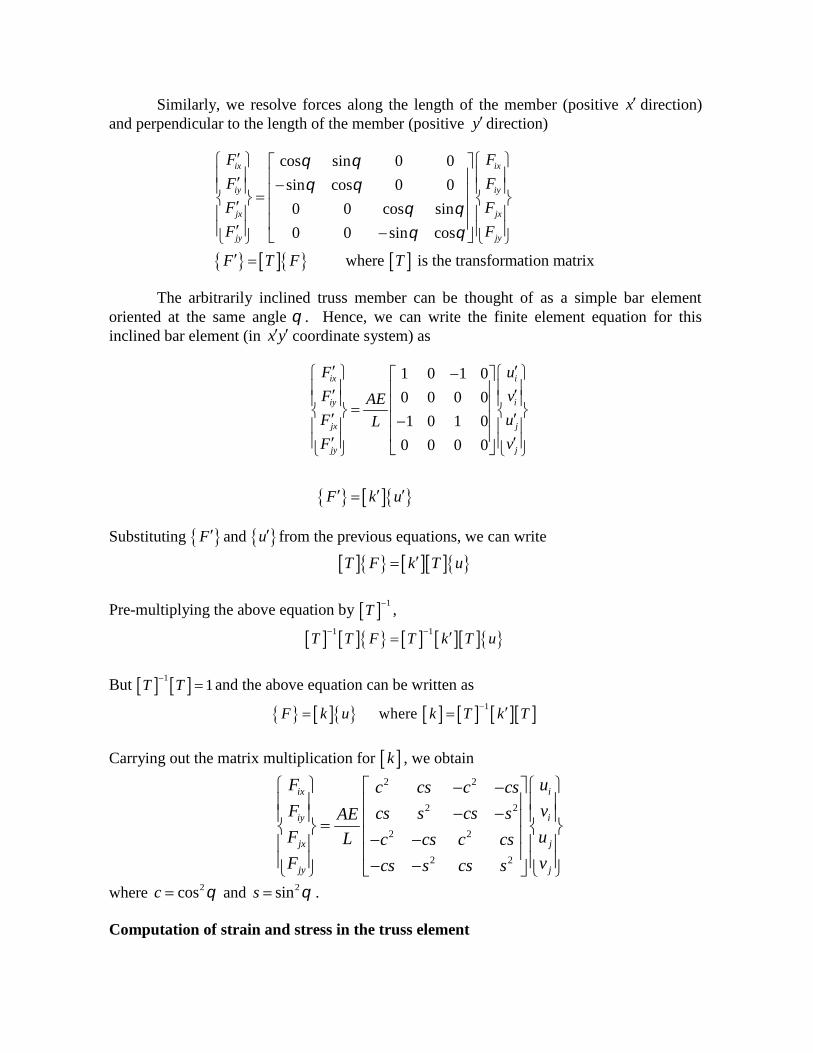
Similarly, we resolve forces along the length of the member (positive x direction)and perpendicular to the length of the member (positive ydirection)
cos sin 0 0
sin cos 0 0
0 0 cos sin
0 0 sin cos
where is the transformation matrix
ix ix
iy iy
jx jx
jy jy
F F
F F
F F
F F
F T F T
The arbitrarily inclined truss member can be thought of as a simple bar elementoriented at the same angle . Hence, we can write the finite element equation for thisinclined bar element (in x y coordinate system) as
1 0 1 0
0 0 0 0
1 0 1 0
0 0 0 0
ix i
iy i
jx j
jy j
F u
F vAEF uL
F v
F k u
Substituting F and u from the previous equations, we can write
T F k T u
Pre-multiplying the above equation by 1T
,
1 1T T F T k T u
But 11T T
and the above equation can be written as
1 whereF k u k T k T
Carrying out the matrix multiplication for k , we obtain2 2
2 2
2 2
2 2
ix i
iy i
jx j
jy j
F uc cs c csF vcs s cs sAEF uL c cs c csF vcs s cs s
where 2cosc and 2sins .
Computation of strain and stress in the truss element

The change in length of the truss member is equal to the change in axial displacement of thetruss member in the x y co-ordinate system
cos sin cos sin
cos sin cos sin
j i
j j i i
i
i
j
j
u u
u v u v
u
v
u
v
Strain in the truss element is given by e
L
, i.e.,
cos sin cos sini
ie
j
j
u
v
uL
v
Stress in the truss element is given by e eE , i.e.,
cos sin cos sini
ie
j
j
u
vE
uL
v
Problem
The two-element truss is subjected to external loading as shown in figure. Using thesame node and element numbering as shown in figure, determine the displacementcomponents at node 3, the reaction components at nodes 1 and 2, and the elementdisplacement, stresses and forces. The elements have modulus of elasticity E1 = E2 = 10×10⁶
2
lb
inand cross-sectional areas A1 = A2 = 1.5 2in
(0,0)
2
(0, 40) ② 300 lb 500 lb
①
13
(40, 40)

For element 1
For element 2
b. Nodal forces
element 1 element 2
iv
6
53
4
①
②31
②
①
2
1
Fix
②i j
ju
i
①
jv
j
3
iv
1
3
Fjx
Finite element modelDegree of freedom
3
1 3
Fiy
Fjy
2
2
1
iu
②i j
jujv

FINITE ELEMENT EQUATION
ix
iy
jx
jy
F
F AEF L
F
2 2
2 2
2 2
2 2
c cs c cs
cs s cs s
c cs c cs
cs s cs s
i
i
j
j
u
v
u
v
For element 1
For element 2
( 2 ) 5
3 4 5 6
31 0 1 0 3 .7 5 0 3 .7 5 0
0 0 0 0 0 0 0 01 0
1 0 1 0 3 .7
4
5
6
5 0 3 .7 5 0
0 0 0 0 0 0 0 0
A EK
L
Assembly of finite element e
1
1
2 5
2
3
3
1 2 3 4 5
1.325 1.325 0 0 1.325 1.325
1.325 1.3
6
1
2
3
4
25 0 0 1.325 1.325
0 0 3.7
5
6
10
x
y
x
y
x
y
F
F
F
F
F
F
1
1
2
2
3
3
5 0 3.75 0
0 0 0 0 0 0
1.325 1.325 3.75 0 5.0751 1.325
1.325 1.325 0 0 1.325 1.325
u
v
u
v
u
v
quation
ixF
65
2
1 .5 1 0 1 04 5, 2 .6 5 1 6 5 1 0
5 6 .5 6 8 5
A E lb
L in
651.5 10 10
0, 3 .75 1040
A E
L
(1)
1 2 5
0.5 0.5 0.5 0.5
0.5 0.5 0.5 0.5
0.5 0.5 0.5 0.5
0.
6
AEK
L
5
1.325826 1.325826 1.325826 1.325826
1.325826 1.325826 1.325826 1.32582610
1.325826 1.325826 1.325826 1.325826
5 0.5 0.5 0.5 1.325826 1.325826 1.325826 1.32
1
2
5
6 5826

Applying boundary conditions knowns unknowns
1
1
2 5
2
1.325826 1.325826 0 0 1.325826 1.325826
1.325826 1.325826 0 0 1.325826 1.325826
0 0 3.75 0 3.75 010
0 0 0 0 0 0
1.325826 1.325826 3.75 0 5.0751826 1.3258265001.325826 1.325826 0 0 1.3258300
x
y
x
y
F
F
F
F
3
3
0
0
0
0
26 1.325826
u
v
Eliminating the 1st, 2nd, 3rd and 4th column to solve 3 3 andu v
53 3500 10 5.075 1.325u v ①
53 3300 10 1.325 1.325u v ②
Solve the equation①and②
Finding element stresses
For element 1
43 5.33 10u in
33 1.731 10v in
1
1
2
2
3
3
x
y
x
y
F
F
F
F
u
v
3
3
1
1
2
2
500 lb
300 lb
0
0
0
0
x
y
F
F
u
v
u
v
3
3
1
2
1
2
500 lb
300 lb
0
0
0
0
x
y
F
F
u
u
v
v
1
1
2
2
300
300
200
0
x
y
x
y
F lb
F lb
F lb
F

6
1 5 3 2
10 10[ cos 0 sin 0 ] (0.5333 1) (0 0) 133.325
40
E lbu u
L in
2 5 6 1 2( cos 45 sin 45 ) ( cos 45 sin 45 )E
u u u uL
63 310 10
(0.5333 10 cos 45 ) (1.731 10 sin 45 ) 056.57
6
2
10 100.0003771 0.001224 283.03
56.57
lb
in
PROBLEM
To illustrate how we can combine spring and bar element in one structure, we cansolve the two-bar truss supported by a spring as shown below. Both bars have E = 210 GPaand A = 5.0 x10⁻⁴ m2. Bar one has a length of 5 m and bar two a length of 10 m. the springstiffness is k = 2000 kN/m.
Solution :Given : E = 210 GPa
A = 5.0 x10⁻⁴ m2 , L1 = 5 m, L2 = 10 m, K = 2 x 1062
N
m
NOTE: A spring is considered as a bar element whose stiffness is 2 x 1062
N
m
1
2
3
4
45o
5m
10m
25kN
1
2
3 k=2000 kN/m

STEP 1 : Finite Element Representation Of Forces And Displacements
Displacements
Total # Of Degrees Of Freedom: 8
Forces
Step 2: Finite Element Equations
Element 1:θ=1350
l2=cos2θ =0.5m2=sin2θ =0.5lm=cosθ sinθ =-0.5
1
1
2
3
2
3
4
F1X
F1Y
F2X
F2Y
F3X
F3Y
F4X
F4Y
1
1
2
3
2
3
4
u1
v1
u2
v2
u3
v3
u4
v4
1
2
3
4
5
6
7
8
1
1
2
135O
x

1
2
3
180O
x
4 2 6 2(1)
1 2 3 4
1 0.5 0.5 0.5 0.55 10 m 210 10 kN/m 2 0.5 0.5 0.5 0.5
3 0.5 0.5 0.5 0.55 m
4 0.5 0.5 0.5 0.5
K
(1) 5
1 2 3 4
1 1 1 1 1
2 1 1 1 1105 10
3 1 1 1 1
4 1 1 1 1
K
Element 2:θ=1800
l2=cos2θ =1m2=sin2θ =0lm=cosθ sinθ =0
Element 3:θ=2700
l2=cos2θ =0m2=sin2θ =1lm=cosθ sinθ =0
4 2 6 2(2)
(2) 5
1 2 5 6
1 1 0 1 05 10 m 210 10 kN/m 2 0 0 0 0
3 1 0 1 010 m
4 0 0 0 0
1 2
1 0 1 0
0 0 0 0105 10
1 0 1 0
0
5 6
1
2
5
6 0 0 0
K
K

(3) 6
1 2 7 8
1
2
7
8
0 0 0 0
0 1 0 110
0 0 0 0
0 1 0 1
K
STEP 3: Combination Of Finite Element Equations
STEP 4: Applying Boundary Conditions:Since nodes 1, 2, and 3 are fixed, we have
u2 = v2 = 0; u3 = v3 = 0; u4 = v4 = 0;
F1x = 0 and F1y = -25 kN
1
1
2
2 5
3
3
4
4
1 2 3 4 5 6 7 8
1
2
210 105 105 105 105 0 0 0
105 125 105 105 0 0 0 20
105 105 105 105 0 0 0 0
105 108 105 105 0 0 0 010
105 0 0 0 105 0 0 0
3
4
5
6
7
8
0 0 0
X
Y
X
Y
X
Y
X
Y
F
F
F
F
F
F
F
F
1
1
2
2
3
3
4
4
0 0 0 0 0
0 0 0 0 0 0 0 0
0 20 0 0 0 0 0 20
u
v
u
v
u
v
u
v
1
1
2
2 5
3
3
4
4
0 210 105 105 105 105 0 0 0
25 105 125 105 105 0 0 0 20
105 105 105 105 0 0 0 0
105 108 105 105 0 0 0 010
105 0 0 0 105 0 0 0
0 0 0 0 0 0 0 0
0 0 0 0 0 0 0 0
0 20 0 0 0 0 0 20
X
Y
X
Y
X
Y
u
v
F
F
F
F
F
F
0
0
0
0
0
0

Check whether there are as many unknowns as knowns.
STEP 5: SOLVING THE EQUATIONS:
Reduced matrix:
15
1
0 210 10510
25 105 125
u
v
On solving,u1=-1.724 x 10⁻³ m v1=-3.4482 x 10⁻³ m
Find the reactions at supports by substituting the known nodal valuesF2x = -18.104 kN F2y = 18.1041 kN
F3x = 18.102 kN F3y = 0
F4x = 0 F4y = 6.89 kN
STEP 6: Post ProcessingStress in element 1:
(1) 3
1.724
3.4482σ 10
0
0
El m l m
L
(1) 51.2 MPa (Tensile)
Stress in element 2:
(1) 3
1.724
3.4482σ 10
0
0
El m l m
L
PROBLEM
A circular concrete beam structure is loaded as shown. Find the deflection of pointsat 8”,16”, and the end of the beam. E = 4 x 10⁶ psi
(2) 36.2 MPa (Compressive)

y
12 in 3 in 50000 lbx
24 in
Solution
The beam structure looks very different from a spring. However, its behavior isvery similar. Deflection occurs along the x-axis only. The only significant differencebetween the beam and a spring is that the beam has a variable cross-sectional area. Anexact solution can be found if the beam is divided into an infinite number of elements,then, each element can be considered as a constant cross-section spring element, obeyingthe relation F = ku, where k is the stiffness constant of a beam element and is given byk = AE/L.
In order to keep size of the matrices small (for hand- calculations), let us divide thebeam into only three elements. For engineering accuracy, the answer obtained will be inan acceptable range. If needed, accuracy can be improved by increasing the number ofelements.
As mentioned earlier in this chapter, spring, truss, and beam elements are line-elements and the shape of the cross section of an element is irrelevant. Only the cross-sectional area is needed (also, moment of inertia for a beam element undergoing abending load need to be defined). The beam elements and their computer models areshown
Here, the question of which cross-sectional area to be used for each beam sectionarises. A good approximation would be to take the diameter of the mid-section and usethat to approximate the area of the element.
k1 k2 k3
1 2 3
k1 k2 k3
1 2 2 3 3 4

Cross-sectional areaThe average diameters are: d1 = 10.5 in., d2 = 7.5 in., d3 = 4.5. (diameters are taken at themid sections and the values are found from the height and length ratio of the trianglesshown in figure 2.10), which is given as
12/L = 3/(L-24), L = 32
Average areas are:
A1 = 86.59 in2 A2 = 56.25 in2 A3 = 15.9 in2
24 in
12 in d1 d2 d3
3 in
Original Averaged 8 8 8 L- 24
L
Stiffness
k1 = A1 E/L1 = (86.59)(4 × 10⁶/8) = 4.3295 ×10⁷ lb./in., similarly,
k2 = A2 E/L2 = 2.8125 ×10⁷ lb./in.k3 = A3 E/L3 = 7.95 ×10⁶ lb./in.
Element Stiffness Equations
[K(1)] = 43.295 × 10⁷ 1 -1-1 1
Similarly,
[K(2)] = 28.125 × 10⁶ 1 -1-1 1
[K(3)] = 7.9500 × 10⁶ 1 -1-1 1

Global stiffness matrix is
43.295 -43.295 0 0[Kg] = -43.295 43.295+28.125 -28.125 0 106
0 -28.125 28.125+7.95 -7.950 0 -7.95 7.95
Now the global structural equations can be written as,
43.295 -43.295 0 0 u1 F1106 -43.295 71.42 -28.125 0 u2 = F2
0 -28.125 36.075 -7.95 u3 F30 0 -7.95 7.95 u4 F4
Applying the boundary conditions: u1 = 0, and F1 = F2 = F3 = 0, F4 = 5000 lb., results inthe reduced matrix,
71.42 -28.125 0 u2 0106 -28.125 36.075 -7.95 u3 = 0
0 -7.95 7.95 u4 5000
Solving we get,
u2 0.0012
u3 = 0.0029 in.u4 0.0092
The deflections u2, u3, and u4 are only the approximate values, which can beimproved by dividing the beam into more elements. As the number of elements increases,the accuracy will improve.

UNIT IV
DYNAMIC ANALYSIS USING ELEMENT METHOD
4.1 INTRODUCTION
It provides the basic equations necessary for structural dynamical analysis and developedboth the lumped and the consistent mass matrix involved in the analysis of bar beam and springelements.
4.1.1 Fundamentals of Vibration
Any motion which repeats itself after an interval of time is called vibration or oscillation orperiodic motion
All bodies possessing mass and elasticity are capable of producing vibration.
4.1.2 Causes of Vibrations
o Unbalanced forces in the machine. These force are produced from within the machineitself
o Elastic nature of the system.o Self excitations produced by the dry friction between the two mating surfaces.o External excitations applied on the system.o Wind may causes vibrationso Earthquakes may causes vibrations
4.1.3 Types of Vibrations
1.According to the actuating force
Free or natural vibrations
Forced vibrations
Damped vibrations
Undamped vibrations
2.According to motion of system with respect to axis
Longitudinal vibrations
Transverse vibrations
Torsional vibrations
ME6603 Finite Element Analysis

4.2 EQUATION OF MOTION
There is two types of equation of motion
Longitudinal vibration of beam or axial vibration of a rod
Transverse vibration of a beam
z y
Mid surface 43
x
1 2
w1 ,w
,w t
x 1 y1
w ww2 , ,
x 2 y2
DOF at each node: w, vw
,y
w.
y
On each element, the deflection w(x,y) is represented by
w(x, y)Ni wii 1
Nxi ( w
x)i
Nyi ( w
y)i ,
where Ni, Nxi and Nyi are shape functions. This is an incompatible element! The
stiffness matrix is still of the form
k = BTEBdV ,where B is the strain-displacement matrix, and E the stress- strain matrix.
Minding Plate Elements:
4-Node Quadrilateral 8-Node Quadrilateral

Three independent fields.Deflection w(x,y) is linear for Q4, and quadratic for Q8.
Discrete Kirchhoff Element:
Triangular plate element (not available in ANSYS). Start with a 6-node riangular element,
z y 3
4 6
1 2t 5
DOF at corner nodes: w,
x
w,
w, , ;
x yx y
DOF at mid side nodes: Total DOF
= 21.
Then, impose conditions
x , y .
xzyz
0, etc., at selected
nodes to reduce the DOF (using relations in (15)). Obtain:
z y 3
1 2x
At each node: w, xw
,x
yw
.y
Total DOF = 9 (DKT Element).
Incompatible w(x,y); convergence is faster (w is cubic along each edge) and it is efficient.

Test Problem:
z
P
yC
L
Lx L/t = 10, = 0.3
ANSYS 4-node quadrilateral plate element.
ANSYS Result for wc
Mesh wc ( PL2/D)2 24 48 8
16 16:
Exact Solution
0.005930.005980.005740.00565
:0.00560
Question:Converges from “above”? Contradiction to what we learnt about the nature ofthe FEA solution?
Reason: This is an incompatible element ( See comments on p. 177).
Shells and Shell Elements
Shells – Thin structures witch span over curved surfaces.

Example:
Sea shell, egg shell (the wonder of the nature); Containers, pipes, tanks;
Car bodies;
Roofs, buildings (the Superdome), etc.Forces in shells:
Membrane forces + Bending Moments
(cf. plates: bending only)
Example: A Cylindrical Container.
internal forces:
p p
membrane stressesdominate

u
Shell Theory:Thin shell theory
Shell theories are the most complicated ones to formulate and analyze in mechanics(Russian’s contributions).
Engineering Craftsmanship Demand strong analytical skill
Shell Elements:
+
plane stress element plate bending element
flat shell element
cf.: bar + simple beam element => general beam element.
DOF at each node:
wv
u x
y
Q4 or Q8 shell element.
Curved shell elements:
zi w
v
ix
y

Based on shell theories;Most general shell elements (flat shell and plate elements are subsets);Complicated in formulation.
Test Cases:
q
R A
80o
L/2
R
L/2
F
A
Roof
F
Pinched Cylinder
F2
F R Fb
A
A F LF1
F
Pinched Hemisphere
4.3CONSISTENT MASS MATRICES
Natural frequencies and modes
Frequency response (F(t)=Fo sinwt) Transient
response (F(t) arbitrary)
F(t)
4.3.1 Single DOF System
k
f=f(t)m - mass
m k - stiffnessc c - damping

Free Vibration:f(t) = 0 and no damping (c = 0)
Eq. (1) becomes
mu ku(meaning: inertia force + stiffness force = 0)
Assume:
u(t) U sin (wt) ,where is the frequency of oscillation, U the amplitude.
Eq. (2) yields
Uù2
m sin( ùt) kU sin( ùt) 0
i.e., w2
m k U 0.
For nontrivial solutions for U, we must have
w2
m k 0,
which yields
wk
m.
This is the circular natural frequency of the single DOF system (rad/s). The cyclic frequency(1/s = Hz) is
wf ,
2p

u = U s in w tU
Ut
T = 1 / f
U n d a m p e d F r e e V i b r a t i o n
With non-zero damping c, where
0 c cc 2mw 2 k m (cc = critical damping)
we have the damped natural frequency:
wd
where x
w 1 x2
,
c(damping ratio).
cc
For structural damping: 0 x 0.15 (usually 1~5%)
wd w.
Thus, we can ignore damping in normal mode analysis.
u
t
Damped Free Vibration

1 2
4.3.2.Multiple DOF System
Equation of Motion
Equation of motion for the whole structure is
Mu Cu Ku f (t) , (8)
in which: u nodal displacement vector,
M mass matrix,
C damping matrix,
K stiffness matrix,
f forcing vector.
Physical meaning of Eq. (8):
Inertia forces + Damping forces + Elastic forces
= Applied forces
Mass Matrices
Lumped mass matrix (1-D bar element):
rAL 1 r,A,L 2 rAL
2 u1 u2
Element mass matrix is found to be
rAL
m 2
0
0
rAL2
diagonal atrix

Simple Beam Element:
v 1
q 1
v2
r, A, L q 2
m rNT NdVV
156 22L 542
13L2
V1
rAL
420
22L
54
13L
4L
13L
3L2
13L
156
22L
3L
22L
4L2
Q1
v2Q2
Units in dynamic analysis (make sure they are consistent):
Choice I Choice IIt (time)
L (length)m (mass)a (accel.)f (force)
r (density)
smkg
m/s2
Nkg/m3
smmMg
mm/s2
NMg/mm3
4.4 VECTOR ITERATION METHODS
Study of the dynamic characteristics of a structure:
natural frequencies normal modes shapes)
Let f(t) = 0 and C = 0 (ignore damping) in the dynamic equation (8) and obtain

2
Mu Ku 0
Assume that displacements vary harmonically with time, that is,
u (t ) u sin( w t ),
u (t ) w u cos( w t ),
u (t )w
2u sin( w t ),
where u is the vector of nodal displacement amplitudes.
Eq. (12) yields,
K w2
M u 0
This is a generalized eigenvalue problem (EVP).
Solutions?
This is an n-th order polynomial of from which we can find n solutions (roots) oreigenvalues
i (i = 1, 2, …, n) are the natural frequencies (or characteristic frequencies) of the
structure (the smallest one) is called the fundamental frequency. For each gives one
solution (or eigen) vector
K w i M u i 0 .
u i (i=1,2,…,n) are the normal modes (or natural modes, mode shapes, etc.).

u
u
i j
M ui j
v2
r, A, EI q2
1 2L
Properties of Normal Modes
TK u 0 ,
T0 , for i ¹j,
if wi wj . That is, modes are orthogonal (or independent) to each other with respect to K and
M matrices.
Note:
Magnitudes of displacements (modes) or stresses in normal mode analysis have no physicalmeaning.
For normal mode analysis, no support of the structure is necessary.
i = 0 there are rigid body motions of the whole or a part of the structure. apply this to check
the FEA model (check for mechanism or free elements in the models).
Lower modes are more accurate than higher modes in the FE calculations (less spatial variationsin the lower modes fewer elements/wave length are needed).
Example:
K w2
M
KEI 12
L3

q 2 1
q 2 2
EVP: 12 156l
6L 22Ll
6L
4L2
22Ll0,
4L2l
in which l w2
rAL4 / 420 EI .
Solving the EVP, we obtain,1
#3 #2
w1 3.533 EI 2 v2,
rAL4
1
1.38 ,
L
1
#1
Exact solutions:
w2 34.81
1
EI2 v2
,rAL
4
1
1
7.62 .
L
w1 3.516 EI2
,rAL
4w2 22.03 EI
2
.rAL
4
4.5 MODELLING OF DAMPING
Two commonly used models for viscous damping.
4.5.1 Proportional Damping (Rayleigh Damping)
C M K(17)
where the constants & are found from
with1 , 2 , 1 & 2 (damping ratio) being selected.

Dam
ping
ratio
u
u
K
M
u
u
0
0
,
,
u M u 1,
u K u ,
i i
Modal Damping
Incorporate the viscous damping in modal equations.
Modal EquationsUse the normal modes (modal matrix) to transform the coupled system ofdynamic equations to uncoupled system of equations.
We have
K2
M u 0 , i 1,2,..., n(18)
where the normal mode u i satisfies:
Ti jT for i j,
i j
andTi i
T 2i i i
for i = 1, 2, …, n.

z p
Form the modal matrix:
Ö ( n n ) u 1 u 2 L u n
are called principal coordinates.
Substitute (21) into the dynamic equation:
M &z& C z& K z f ( t ).
Pre-multiply byT
, and apply (20):
&z& C
where C
p
z& z
I
Tf ( t ) .
p ( t ),
(proportional damping),
Using Modal Damping
Can verify that
Transformation for the displacement vector,
z1 (t) z2 (t) M
zn (t)
Equation (22) becomes,
&z&i 2 i i z&i2i ii
( t ),i = 1,2,…,n. (24)
Equations in (22) or (24) are called modal equations. These are uncoupled, second-order differential equations, which are much easier to solve than the original dynamicequation (coupled system).
To recover u from z, apply transformation (21) again, once z is obtained from (24).

z
)z i
2
i i )i
Notes:
Only the first few modes may be needed in constructing the modal matrix (i.e.,could be an n m rectangular matrix with m<n). Thus, significant reduction in the
size of the system can be achieved.
Modal equations are best suited for problems in which higher modes are notimportant (i.e., structural vibrations, but not shock loading).
4.5.2 Frequency Response Analysis
(Harmonic Response Analysis)
Ku E uHarmonicloading
(25)
Modal method: Apply the modal equations,
&z&i 2 i i Zk i i i pisin t ,
i=1,2,…,m. (26)
These are 1-D equations. Solutions are
p 2zi (t) i i sin( t
(1
where
2 2(2
2
/ ii
ci ci , damping ratio
cc 2m i
Recover u from (21).
Direct Method: Solve Eq. (25) directly, that is, calculate
the inverse. With u
becomesu e
i t(complex notation), Eq. (25)
This equation is expensive to solve and matrix is ill- conditioned if is close

4.6TRANSIENT RESPONSE ANALYSIS
(Dynamic Response/Time-History Analysis)
Structure response to arbitrary, time-dependent loading.
f(t)
t
u(t)
t
Compute responses by integrating through time:
u 1
u n u n+1u 2
t 0 t 1 t 2 t n t n+1B. Modal Method
First, do the transformation of the dynamic equations using the modal matrix before thetime marching:
Then, solve the uncoupled equations using an integration method. Can use, e.g.,10%, of the total modes (m= n/10).
Uncoupled system, Fewer equations,
No inverse of matrices,More efficient for large problems.

4.6.1Cautions in Dynamic AnalysisSymmetry: It should not be used in the dynamic analysis (normal modes, etc.)because symmetric structures can have antisymmetric modes.
Mechanism, rigid body motion means = 0. Can use this to check FEA modelsto see if they are properly connected and/or supported.
Input for FEA: loading F(t) or F( ) can be very complicated in real applicationsand often needs to be filtered first before used as input for FEA.
ExamplesImpact, drop test, etc.
PROBLEM
In the spring structure shown k1 = 10 lb./in., k2 = 15 lb./in., k3 = 20 lb./in., P= 5 lb.Determine the deflection at nodes 2 and 3.
k1 k2 k3
o o o o1 2 3 4
Figure 2.4
Solution:
Again apply the three steps outlined previously.
Step 1: Find the Element Stiffness Equations
Element 1:1 2
[K(1)] = 10 -10 1-10 10 2
Element 2: 2 3[K(2)] = 15 -15 2
-15 15 3
Element 3: 3 4
[K(3)] = 20 -20 3
-20 20 4

Step 2: Find the Global stiffness matrix
1 2 3 41 10 -10 0 0 10 -10 0 02 -10 10 + 15 -15 0 = -10 25 -15 03 0 -15 15 + 20 -20 0 -15 35 -204 0 0 -20 20 0 0 -20 20
Now the global structural equation can be written as,
F1 10 -10 0 0 u1
F2 = -10 25 -15 0 u2
F3 0 -15 35 -20 u3
F4 0 0 -20 20 u4
Step 3: Solve for Deflections
The known boundary conditions are: u1 = u4 = 0, F3 = P = 3lb. Thus, rows and columns 1 and 4 will dropout, resulting in the following matrix equation,
03 = 25 −15−15 35 = 23Solving, we get u2 = 0.0692 & u3 = 0.1154
PROBLEMIn the spring structure shown, k1 = 10 N/mm, k2 = 15 N/mm, k3 = 20 N/mm, k4 = 25 N/mm, k5 = 30
N/mm, k6 = 35 N/mm. F2 = 100 N. Find the deflections in all springs.
k1
k3
k2 F2 k6
k4
k5

Solution:
Here again, we follow the three-step approach described earlier, without specificallymentioning at each step.
Element 1: 1 4[K(1)] = 10 -10 1
-10 10 4
Element 2: 1 2
[K(2)] = 15 -15 1
-15 15 2
Element 3: 2 3
[K(3)] = 20 -20 2
-20 20 3
Element 4:[K(4)] =
225
3-25 2
-25 25 3
Element 5: 2 4
[K(5)] = 30 -30 2
-30 30 4
Element 6: 3 4
[K(6)] = 35 -35 3
-35 35 4
The global stiffness matrix is,
1 2 3 4
10+15 -15 0 -10 1
[Kg] = -15 15+20+25+30 -20-25 -30 2
0 -20-25 20+25+35 -35 3
-10 -30 -35 10+30+35 4
And simplifying, we get
25 -15 0 -10[Kg] = -15 90 -45 -30
0 -45 80 -35-10 -30 -35 75

And the structural equation is,
F1 25 -15 0 -10 u1
F2 = -15 90 -45 -30 u2
F3 0 -45 80 -35 u3
F4 -10 -30 -35 75 u4
Now, apply the boundary conditions, u1 = u4 = 0, F2 = 100 N. This is carried out bydeleting the rows 1 and 4, columns 1 and 4, and replacing F2 by 100N. The final matrixequation is,
Which gives
Deflections:
Spring 1: u4 – u1 = 0
Spring 2: u2 – u1 = 1.54590
Spring 3: u3 – u2 = -0.6763
Spring 4: u3 – u2 = -0.6763
Spring 5: u4 – u2 = -1.5459
Spring 6: u4 – u3 = -0.8696
100 90 -45 u2
0 = -45 80 u3

UNIT V
APPLICATIONS IN HEAT TRANSFER &FLUID MECHANICS
5.1 ONE DIMENSIONAL HEAT TRANSFER ELEMENT
In structural problem displacement at each nodel point is obtained. Byusing these displacement solutions, stresses and strains are calculated for eachelement. In structural problems, the unknowns are represented by thecomponents of vector field. For example, in a two dimensional plate, theunknown quantity is the vector field u(x,y),where u is a (2x1)displacementvector.
Heat transfer can be defined as the transmission of energy from oneregion another region due to temperature difference. A knowledge of thetemperature distribution within a body is important in many engineeringproblems. There are three modes of heat transfer.
They are: (i) Conduction
(ii) Convection
(iii) Radiation
5.1.1Strong Form for Heat Conduction in One Dimensionwith Arbitrary Boundary Conditions
Following the same procedure as in Section, the portion of theboundary where the temperature is prescribed, i.e. the essential boundary isdenoted by T and the boundary where the flux is prescribed is recommendedfor Science and Engineering Track. Denoted by q ; these are theboundaries with natural boundary conditions. These boundaries arecomplementary, so
q = ¼ ; q \ T ¼ 0:
With the unit normal used in , we can express the natural boundarycondition as qn ¼ q. For example, positive flux q causes heat inflow (negativeq ) on the left boundary point where qn ¼ q ¼ q and heat outflow (positiveq ) on the right boundary point where qn ¼ q ¼ q.
Strong form for 1D heat conduction problems

5.1.2Weak Form for Heat Conduction in One Dimension withArbitrary Boundary Conditions
We again multiply the first two equations in the strong form by the weightfunction and integrate over the domains over which they hold, the domain for thedifferential equation and the domain q for the flux boundary condition, whichyields ws dx with w ¼Recalling that w ¼ 0 on T and combining with gives
Weak form for 1D heat conduction problemsFind T ðxÞ 2 U such that
Notice the similarity between
5.2 APPLICATION TO HEAT TRANSFER TWO-DIMENTIONAL
5.2.1Strong Form for Two-Point Boundary Value Problems
The equations developed in this chapter for heat conduction, diffusion andelasticity problems are all of the following form:
Such one-dimensional problems are called two-point boundary valueproblems. gives the particular meanings of the above variables and parametersfor several applications. The natural boundary conditions can also begeneralized as (based on Becker et al. (1981))
Þ ¼ 0 on :
Equation is a natural boundary condition because the derivative of thesolution appears in it. reduces to the standard natural boundary conditionsconsidered in the previous sections when bðxÞ ¼ 0. Notice that the essentialboundary condition can be recovered as a limiting case of when bðxÞ is apenalty parameter, i.e. a large number In this case, and Equation iscalled a generalized boundary condition.
An example of the above generalized boundary condition is an elastic barwith a spring attached as shown in In this case, bðlÞ ¼ k and reduces to
E(n-l) ( k-uð) uÞ ¼ 0 at x ¼ l;

where ¼ k is the spring constant. If the spring stiffness is set to a very largevalue, the above boundary condition enforces ¼ u; if we let k ¼ 0, the aboveboundary condition corresponds to a prescribed traction boundary. In practice,such generalized boundary conditions are often used to model the influence ofthe surroundings. For example, if the bar is a simplified model of a building and itsfoundation, the spring can represent the stiffness of the soil.
5.2.2 Two-Point Boundary Value Problem With Generalized BoundaryConditions
- ku(l)
u(l)u k
t
An example of the generalized boundary for elasticity problem.
Another example of the application of this boundary condition isconvective heat transfer, where energy is transferred between the surface of thewall and the surrounding medium. Suppose convective heat transfer occurs at x¼ l. Let T ðlÞ be the wall temperature at x ¼ l and T be the temperature in themedium. Then the flux at the boundary x ¼ l is given by qðlÞ ¼ hðT ðlÞ T Þ, sobðlÞ ¼ h and the boundary condition is
where h is convection coefficient, which has dimensions of W m 2 o
C 1 . Note that when the convection coefficient is very large, the temperatureT is immediately felt at x ¼ l and thus the essential boundary condition isagain enforced as a limiting case of the natural boundary condition.
There are two approaches to deal with the boundary condition . We willcall them the penalty and partition methods. In the penalty method, theessential boundary condition is enforced as a limiting case of the naturalboundary condition by equating bðxÞ to a penalty parameter. The resultingstrong form for the penalty method is given in.
General strong form for 1D problems-penalty method
þ f ¼ 0 on ;

STRONG AND WEAK FORMS FOR ONE-DIMENSIONAL PROBLEMS
In the partition approach, the total boundary is partitioned into the naturalboundary, and the complementary essential boundary, The natural boundary condition hasthe generalized form defined by The resulting strong form for the partition method issummarized in.
5.2.3 Weak Form for Two-Point Boundary Value Problems
In this section, we will derive the general weak form for two-point boundary valueproblems. Both the penalty and partition methods described in will be considered. Toobtain the general weak form for the penalty method, we multiply the two equations in thestrong by the weight function and integrate over the domains over which they hold: thedomain for the differential equation and the domain for the generalized boundarycondition.
5.3 SCALE VARIABLE PROBLEM IN 2 DIMENSIONS
x1 y2 x1
x N1
u 0 N2 0 N3 0 N4 0 y2
y 0 N1 0 N2 0 N3 0 N4 x3
y 3 x4 y4
N1=1/4(1-Ɛ) (1-ɳ); N2=1/4(1+Ɛ) (1-ɳ); N3=1/4(1+Ɛ) (1+ɳ); N4=1/4(1-Ɛ) (1+ɳ).
Equation of Stiffness Matrix for 4 noded isoparametric quadrilateral element
J J11 J12 ;
J 21 J 22

STRONG AND WEAK FORMS FOR ONE-DIMENSIONAL PROBLEMS
0
0
0
B 1
J
J 22
J12
0
0
J 21
0
J11
N1
N1
0
0
N1
N 2
N 2
0
0
N 2
N3
N3
0
0
N3
N 4
N 4
0
N 4
J 21 J11 J 22 J12 0
0
0 0
0N1 0
N 2 0N3 0
N4
E 1 v v
[D] v 1 0 (1 v2 )
01 v , for plane stress conditions;
0
E 1 v
2
v 0 [D] v 1 v 0
(1 v)(1 2v) 0
1 2v , for plane strain conditions.0 2
Equation of element force vector
F F [N ]T xe F ;
y
N – Shape function, Fx – load or force along x direction,
Fy – load or force along y direction.
Numerical Integration (Gaussian Quadrature)
The Gauss quadrature is one of the numerical integration methods to calculate the
definite integrals. In FEA, this Gauss quadrature method is mostly preferred. In
this method the numerical integration is achieved by the following expression,
1 n
f (x)dx wi f (xi )1 i1
Table gives gauss points for integration from -1 to 1.

Number of
Points
n
Location
xi
Corresponding Weights
wi
1 x1 = 0.000 2.000
2 1x1, x2 = 0.577350269189
3 1.000
3x1, x3
3 0.774596669241
5
x2=0.000
5 0.555555
9
8 0.888888
9
4 x1, x4= 0.8611363116
x2, x3= 0.3399810436
0.3478548451
0.6521451549
Problem (I set)
1 x1. Evaluate I cos
1 2dx , by applying 3 point Gaussian quadrature and
compare with exact solution.
1 1 2. Evaluate I 3e x x2
1 x 2dx , using one point and two point
Gaussian quadrature. Compare with exact solution.
3. For the isoparametric quadrilateral element shown in figure, determine the
local co –ordinates of the point P which has Cartesian co-ordinates (7, 4).

4. A four noded rectangular element is in figure. Determine (i) Jacobian
matrix, (ii) Strain – Displacement matrix and (iii) Element Stresses. Take
E=2x10⁵N/mm2,υ= 0.25, u=[0,0,0.003,0.004,0.006, 0.004,0,0]T, Ɛ= 0, ɳ=0.Assume plane stress condition.
5.4 2 DIMENTIONAL FLUID MECHANICS
The problem of linear elastostatics described in detail in can be extended to include theeffects of inertia. The resulting equations of motion take the form
∇ · σ + f = ρu in Ω ×I ,
σn = t on Γq ×I ,
u = u on Γu ×I ,
u(x1 ,x2 ,x3,0) = u0 (x1,x2 ,x3 ) in Ω ,
v(x1, x2 ,x3,0) = v0 (x1,x2 ,x3) in Ω ,

where u = u(x1 , x2, x3 , t) is the unknown displacement field, ρ is the mass density, and I= (0, T ) with T being a given time. Also, u0 and v0 are the prescribed initial displacementand velocity fields. Clearly, two sets of boundary conditions are set on Γu and Γq ,respectively, and are assumed to hold throughout the time interval I . Likewise, two sets ofinitial conditions are set for the whole domain Ω at time t = 0. The strong form of theresulting initial/boundary- value problem is stated as follows: given functions f , t , u , u0 andv0, as well as a constitutive equation for σ, find u in Ω × I , such that the equations aresatisfied.
A Galerkin-based weak form of the linear elastostatics problem has been derived in Sec-tion In the elastodynamics case, the only substantial difference involves the inclusion
of the termR
Ω w · ρu dΩ, as long as one adopts the semi-discrete approach. As a result, the
weak form at a fixed time can be expressed asZ
w · ρu dΩ +Ω
Z∇sw : σ dΩ =
Ω
Z Zw · f dΩ +
Ω Γw · t dΓ .
Following the development of Section 7.3, the discrete counterpart of can be written asZ
wh · ρuh dΩ + ǫ(wh) · Dǫ(uh) dΩ=
Z Zwh · f dΩ +
wh · t dΓ .
Following a standard procedure, the contribution of the forcing vector Fint,e due tointerele- ment tractions is neglected upon assembly of the global equations. As a result, theequations is give rise to their assembled counterparts in the form
Mu + Ku = F ,
where u is the global unknown displacement vector1 . The preceding equations are, of course,subject to initial conditions that can be written in vectorial form as u(0) = u0 and v(0) = v0.
The most commonly employed method for the numerical solution of the system of cou-
pled linear second-order ordinary differential equations is the Newmark method. This
method is based on a time series expansion of u and u := v. Concentrating on the timeinterval (tn , tn+1], the Newmark method is defined by the equations
1 2un+1 =
vn+1 =
un + vn∆tn +2
[(1 − 2β)an + 2βan+1]∆tn ,
vn + [(1 − γ)an + γan+1 ]∆tn ,

n
n
It is clear that the Newmark equations define a whole family of time integrators.
It is important to distinguish this family into two categories, namely implicit and explicitintegrators, corresponding to β > 0 and β = 0, respectively.
The overhead “hat” symbol is used to distinguish between the vector field u and thesolution vector uemanating from the finite element approximation of the vector field u.
The general implicit Newmark integration method may be implemented as follows: first,
solve (9.18)1 for an+1 , namely write
an+1 =β∆t2
(un+1 − un − vn∆tn ) an
Then, substitute (9.19) into the semi-discrete form (9.17) evaluated at tn+1 to find that
M + K un+1 = Fn+1.
After solving for un+1, one may compute the acceleration an+1 from and the velocityvn+1 from.
Finally, the general explicit Newmark integration method may be implemented as follows:starting from the semi-discrete equations evaluated at tn+1, one may substitute un+1fromto find that
Man+1 = −K(un + vn∆tn +an∆tn ) + Fn+1 .
If M is rendered diagonal (see discussion in Chapter 8), then an+1 can be determined
without solving any coupled linear algebraic equations. Then, the velocities bvn+1 areimmediately computed from (9.18)2. Also, the displacements u n+1 are computed fromindepen-dently of the accelerations an+1 .
n
n
It is clear that the Newmark equations define a whole family of time integrators.
It is important to distinguish this family into two categories, namely implicit and explicitintegrators, corresponding to β > 0 and β = 0, respectively.
The overhead “hat” symbol is used to distinguish between the vector field u and thesolution vector uemanating from the finite element approximation of the vector field u.
The general implicit Newmark integration method may be implemented as follows: first,
solve (9.18)1 for an+1 , namely write
an+1 =β∆t2
(un+1 − un − vn∆tn ) an
Then, substitute (9.19) into the semi-discrete form (9.17) evaluated at tn+1 to find that
M + K un+1 = Fn+1.
After solving for un+1, one may compute the acceleration an+1 from and the velocityvn+1 from.
Finally, the general explicit Newmark integration method may be implemented as follows:starting from the semi-discrete equations evaluated at tn+1, one may substitute un+1fromto find that
Man+1 = −K(un + vn∆tn +an∆tn ) + Fn+1 .
If M is rendered diagonal (see discussion in Chapter 8), then an+1 can be determined
without solving any coupled linear algebraic equations. Then, the velocities bvn+1 areimmediately computed from (9.18)2. Also, the displacements u n+1 are computed fromindepen-dently of the accelerations an+1 .

QUESTION BANK
PART A QUESTIONS WITH ANSWERS
1. What is meant by finite element?
UNIT 1
A small units having definite shape of geometry and nodes is called finite element.
2. What is meant by node or joint?
Each kind of finite element has a specific structural shape and is inter- connected with
the adjacent element by nodal point or nodes. At the nodes, degrees of freedom are
located. The forces will act only at nodes at any others place in the element.
3. What is the basic of finite element method?
Discretization is the basis of finite element method. The art of subdividing a structure
in to convenient number of smaller components is known as discretization.
4. What are the types of boundary conditions?
Primary boundary conditions
Secondary boundary conditions
5. State the methods of engineering analysis?
Experimental methods
Analytical methods
Numerical methods or approximate methods
6. What are the types of element?
7. 1D element
2D element
3D element
8. State the three phases of finite element method.
Preprocessing
Analysis
Post Processing
9. What is structural problem?
Displacement at each nodal point is obtained. By these displacements solution
stress and strain in each element can be calculated.

10. What is non structural problem?
Temperature or fluid pressure at each nodal point is obtained. By using these
values properties such as heat flow fluid flow for each element can be calculated.
10. What are the methods are generally associated with the finite element analysis?
Force method
Displacement or stiffness method.
11. Explain stiffness method.
Displacement or stiffness method, displacement of the nodes is considered as the
unknown of the problem. Among them two approaches, displacement method is
desirable.
12. What is meant by post processing?
Analysis and evaluation of the solution result is referred to as post processing.
Postprocessor computer program help the user to interpret the result by displaying
them in graphical form.
13. Name the variation methods.
Ritz method.
Ray-Leigh Ritz method.
14. What is meant by degrees of freedom?
When the force or reaction act at nodal point node is subjected to deformation. The
deformation includes displacement rotation, and or strains. These are collectively
known as degrees of freedom
15. What is meant by discretization and assemblage?
The art of subdividing a structure in to convenient number of smaller components
is known as discretization. These smaller components are then put together. The
process of uniting the various elements together is called assemblage.
16. What is Rayleigh-Ritz method?
It is integral approach method which is useful for solving complex structural
problem, encountered in finite element analysis. This method is possible only if a
suitable function is available.
17. What is Aspect ratio?
It is defined as the ratio of the largest dimension of the element to the smallest
dimension. In many cases, as the aspect ratio increases the in accuracy of the
solution increases. The conclusion of many researches is that the aspect ratio

18. What is truss element?
The truss elements are the part of a truss structure linked together by point jointwhich transmits only axial force to the element.
19. What are the h and p versions of finite element method?
It is used to improve the accuracy of the finite element method. In h version, the
order of polynomial approximation for all elements is kept constant and the numbers of
elements are increased. In p version, the numbers of elements are maintained constant and
the order of polynomial approximation of element is increased.
20. Name the weighted residual method
Point collocation method
Sub domain collocation method
Least squares method
Galerkins method.
UNIT 2
21. List the two advantages of post processing.
Required result can be obtained in graphical form. Contour diagrams can be used to
understand the solution easily and quickly.
22. During discretization, mention the places where it is necessary to place a
node?
Concentrated load acting point
Cross-section changing point
Different material interjections
Sudden change in point load
23. What is the difference between static and dynamic analysis?
Static analysis: The solution of the problem does not vary with time is known as
static analysis
Example: stress analysis on a beam
Dynamic analysis: The solution of the problem varies with time is known as
dynamic analysis

24. Name any four FEA softwares.
ANSYS
NASTRAN
COSMOS
25. Differentiate between global and local axes.
Local axes are established in an element. Since it is in the element level, they change
with the change in orientation of the element. The direction differs from element to
element.
Global axes are defined for the entire system. They are same in direction for all the
elements even though the elements are differently oriented.
26. Distinguish between potential energy function and potential energy functional
If a system has finite number of degree of freedom (q1,q2,and q3), then the potential
energy expressed as,
π = f (q1,q2,and q3)
It is known as function. If a system has infinite degrees of freedom then the potential
energy is expressed as
dy d 2y f x , y , , ....dx 2
dx dx 27. What are the types of loading acting on the structure?
Body force (f)
Traction force (T)
Point load (P)
28. Define the body force
A body force is distributed force acting on every elemental volume of the
body Unit: Force per unit volume.
Example: Self weight due to gravity
29. Define traction force
Traction force is defined as distributed force acting on the surface of the
body. Unit: Force per unit area.
Example: Frictional resistance, viscous drag, surface shear
30. What is point load?
Point load is force acting at a particular point which causes displacement.

31. What are the basic steps involved in the finite element modeling.
Discretization of structure.
Numbering of nodes.
32. Write down the general finite element equation.
F K u
33. What is discretization?
The art of subdividing a structure in to a convenient number of smaller components isknown as discretization.
34. What are the classifications of coordinates?
Global coordinates
Local coordinates
Natural coordinates
35. What is Global coordinates?
The points in the entire structure are defined using coordinates system is known as
global coordinate system.
36. What is natural coordinates?
A natural coordinate system is used to define any point inside the element by a set
of dimensionless number whose magnitude never exceeds unity. This system is
very useful in assembling of stiffness matrices.
37. Define shape function.
Approximate relation φ (x,y) = N1 (x,y) φ1 + N2 (x,y) φ2 + N3 (x,y) φ3
Where φ1, φ2, and φ3 are the values of the field variable at the nodes N1, N2, and
N3 are the interpolation functions.
N1, N2, and N3 are also called shape functions because they are used to express the
geometry or shape of the element.
38. What are the characteristic of shape function?
It has unit value at one nodal point and zero value at other nodal points. The sum of
shape function is equal to one.
39. Why polynomials are generally used as shape function?
Differentiation and integration of polynomial are quit easy.
The accuracy of the result can be improved by increasing the order of the
polynomial. It is easy to formulate and computerize the finite element equations

40. How do you calculate the size of the global stiffness matrix?
Global stiffness matrix size = Number of nodes X Degrees of freedom per node
UNIT 3
41. Write down the expression of stiffness matrix for one dimensional bar element.
AE 1 1K
l 1 1 42. State the properties of stiffness matrix
It is a symmetric matrix
The sum of elements in any column must be equal to zeroIt is an unstable element. So the determinant is equal to zero.
43. Write down the expression of stiffness matrix for a truss element.
u 1
u1 l m 0 0 u
u
2
0 0l mu 2 3
u 4
44. Write down the expression of shape function N and displacement u for one
dimensional bar element.
U= N1u1+N2u2
N1= 1-X /
l N2 = X / l
45. Define total potential energy.
Total potential energy, π = Strain energy (U) + potential energy of the external forces
(W)
46. State the principle of minimum potential energy.
Among all the displacement equations that satisfied internal compatibility and the
boundary condition those that also satisfy the equation of equilibrium make the
potential energy a minimum is a stable system.
47. Write down the finite element equation for one dimensional two noded bar element.
AE 1 1K
l 1 1
48. What is truss?
A truss is defined as a structure made up of several bars, riveted or welded together.

49. States the assumption are made while finding the forces in a truss.
All the members are pin jointed.
The truss is loaded only at the joint
The self weight of the members is neglected unless stated.
50. State the principles of virtual energy?
A body is in equilibrium if the internal virtual work equals the external virtual work
for the every kinematically admissible displacement field
51. What is essential boundary condition?
Primary boundary condition or EBC Boundary condition which in terms of field
variable is known as Primary boundary condition.
52. Natural boundary conditions?
Secondary boundary natural boundary conditions which are in the differential form
of field variable is known as secondary boundary condition
53. How do you define two dimensional elements?
Two dimensional elements are define by three or more nodes in a two dimensional
plane. The basic element useful for two dimensional analysis is the triangular
element.
54. What is CST element?
Three noded triangular elements are known as CST. It has six unknown
displacement degrees of freedom (u1, v1, u2, v2, u3, v3). The element is called
CST because it has a constant strain throughout it.
55. What is LST element?
Six nodded triangular elements are known as LST. It has twelve unknown
displacement degrees of freedom. The displacement function for the elements are
quadratic instead of linear as in the CST.
56. What is QST element?
Ten nodded triangular elements are known as Quadratic strain triangle. It is also
called as cubic displacement triangle.
58. What meant by plane stress analysis?
Plane stress is defined to be a state of stress in which the normal stress and shear
stress directed perpendicular to the plane are assumed to be zero.

60. Define plane strain analysis.
Plane strain is defined to be state of strain normal to the xy plane and the shear
strains are assumed to be zero.
UNIT 4
61. Write down the stiffness matrix equation for two dimensional CST elements.
Stiffness matrix K B T D B At
BT -Strain displacement D-Stress strain matrix B-Strain displacement matrix 62. Write down the stress strain relationship matrix for plane stress conditions.
1 0
E 1 12 0
1
0
12 0 0
2
63. What is axisymmetric element?
Many three dimensional problem in engineering exhibit symmetry about an axis of
rotation such type of problem are solved by special two dimensional element called
the axisymmetric element
64. What are the conditions for a problem to be axisymmetric?
The problem domain must be symmetric about the axis of revolution All
boundary condition must be symmetric about the axis of revolution All
loading condition must be symmetric about the axis of revolution
65. Give the stiffness matrix equation for an axisymmetric triangular
element. Stiffness matrix K B T D B 2rA
66. What is the purpose of Isoparametric element?
It is difficult to represent the curved boundaries by straight edges finite elements. A
large number of finite elements may be used to obtain reasonable resemblance
between original body and the assemblage.
67. Write down the shape functions for 4 noded rectangular elements using natural
coordinate system.

N11 11 N2
1 114 4
N3 1 1 1 N4
11 1 4 4
68. Write down Jacobian matrix for 4 noded quadrilateral elements.
J J J 11 12
J 21
J22
69. Write down stiffnes matrix equation for 4 noded isoparametric quadrilateral elements.
Stiffness matrix K t 1 1 B T D B J 1 1
70. Define super parametric element.
If the number of nodes used for defining the geometry is more than of nodes used
for defining the displacement is known as super parametric element
71. Define sub parametric element.
If the number of nodes used for defining the geometry is less than number of nodes
used for defining the displacement is known as sub parametric element.
72. What is meant by Isoparametric element?
If the number of nodes used for defining the geometry is same as number of nodes
used for defining the displacement is known as Isoparametric element.
73. Is beam element an Isoparametric element?
Beam element is not an Isoparametric element since the geometry and displacement
are defined by different order interpretation functions.
74. What is the difference between natural coordinate and simple natural
coordinate?
L1 = 1-x/l
L2 = x/l
75. What is Area coordinates?
L1 = A1/A L2 = A2/A L3 = A3/A
76. What is simple natural coordinate?
A simple natural coordinate is one whose value between -1 and 1.
77. Give example for essential boundary conditions.
The geometry boundary condition are displacement, slope.

78. Give example for non essential boundary conditions.
The natural boundary conditions are bending moment, shear force
79. What is meant by degrees of freedom?
When the force or reaction act at nodal point node is subjected to deformation. The
deformation includes displacement rotation, and or strains. These are collectively
known as degrees of freedom.
80. What is QST element?
Ten noded triangular elements are known as Quadratic strain triangle. It is also
called as cubic displacement triangle.
UNIT 5
81. What meant by plane stress analysis?
Plane stress is defined to be a state of stress in which the normal stress and shear
stress directed perpendicular to the plane are assumed to be zero.
82. Define plane strain analysis.
Plane strain is defined to be state of strain normal to the x,y plane and the shear
strains are assumed to be zero.
83. What is truss element?The truss elements are the part of a truss structure linked together by point joint
which transmits only axial force to the element.
84. List the two advantages of post processing.
Required result can be obtained in graphical form.
Contour diagrams can be used to understand the solution easily and quickly.
85. What are the h and p versions of finite element method?
It is used to improve the accuracy of the finite element method. In h version, the order
of polynomial approximation for all elements is kept constant and the numbers of
elements are increased. In p version, the numbers of elements are maintained constant
and the order of polynomial approximation of element is increased.

86. During discretization, mention the places where it is necessary to place a node?
Concentrated load acting point Cross-
section changing point Different
material inter junction point Sudden
change in point load
87. What is the difference between static and dynamic analysis?
Static analysis: The solution of the problem does not vary with time is known as
static analysis
Example: stress analysis on a beam
Dynamic analysis: The solution of the problem varies with time is known as
dynamic analysis
Example: vibration analysis problem.
88. What is meant by discretization and assemblage?
The art of subdividing a structure in to convenient number of smaller components is
known as discretization. These smaller components are then put together. The
process of uniting the various elements together is called assemblage.
89. What is Rayleigh-Ritz method?
It is integral approach method which is useful for solving complex structural
problem, encountered in finite element analysis. This method is possible only if a
suitable function is available.
90. What is Aspect ratio?
It is defined as the ratio of the largest dimension of the element to the smallest
dimension. In many cases, as the aspect ratio increases the in accuracy of the solution
increases. The conclusion of many researches is that the aspect ratio should be close
to unity as possible.
91. What is essential boundary condition?
Primary boundary condition or EBC, Boundary condition which in terms of field
variable is known as Primary boundary condition
92. Natural boundary conditions.
Secondary boundary natural boundary conditions which are in the differentialform of field variable is known as secondary boundary condition.
93. How do you define two dimensional elements?
Two dimensional elements are define by three or more nodes in a two dimensional

plane. The basic element useful for two dimensional analysis is the triangular
element.
94. State the principles of virtual energy?
A body is in equilibrium if the internal virtual work equals the external virtual work
for the every kinematically admissible displacement field..
96. What is non-homogeneous form?
When the specified values of dependent variables are non-zero, the boundary
conditi said to be non-homogeneous.
97. What is homogeneous form?
When the specified values of dependent variables is zero, the boundary condition are
said to be homogeneous.
98. Define initial value problem.
An initial value problem is one in which the dependent variable and possibly is
derivatives are specified initially.
99. Define boundary value problem.
A differential equation is said to describe a boundary value problem if the dependent
variable and its derivatives are required to take specified values on the boundary.