Elastoplastic consolidation at finite strain Part 2: Finite element
i
FINITE ELEMENT ALGORITHMS
FOR ELASTOPLASTICITY AND
CONSOLIDATION
by
Andrew John Abbo
B.E, B.Math
A Thesis submitted for the Degree of
Doctor of Philosophy
at the University of Newcastle.
February 1997
(3rdEdition, October 2005)

ii
“I hereby certify that the work embodied in this Thesis is the result of original research
and has not been submitted for a higher degree to any other University or Institute”
(signed)
iii
ACKNOWLEDGEMENTS
The author gratefully acknowledges the financial assistance received through the
receipt of an Australia Postgraduate Award during his candidature. He also is
thankful for the ‘top up’ scholarship provided by the Department of Civil , Surveying
and Environmental Engineering at the University of Newcastle.
The author is indebted to Dr. Scott Sloan for his interest, guidance and provision of
financial assistance during this research. Dr. Sloan’s commitmentand assistancewere
limitless and this is greatly appreciated.
Thanks are also extended to Mr. Peter Kleeman and Dr. Mark Allman for their
valuable time spent proof reading this Thesis.
Finally, thankyou to my wife for her support and encouragement throughout the
period of my studies.
Preface to Third Edition
The third edition of this theis incorprates the minor changes listed below.
¯Minor changes to pagination due to bug in latest version of the publishing
software used in the preparation of the thesis.
¯Correction of some equations in chapter 2.
iv
ABSTRACT
Finite element analysis of nonlinear problems invariably uses piecewise linearisation
to generate approximate solutions. In geomechanics, this linearisation may appear
as:
¯ Discrete strain increments for the integration of nonlinear constitutive laws.
¯ Discrete load increments in nonlinear analyses.
¯ Discrete time steps in the analysis of consolidation.
The size and distribution of these increments (or steps) has a direct bearing on the
accuracy of the resulting solution.
This Thesis describes several new algorithms for controlling the error caused by the
use of discrete increments in nonlinear finite element analysis. The new schemes are
unified by the fact that they all treat the governing relations as a system of ordinary
differential equations. These equations are solved by adaptive integration with
respect to real or pseudo time, and automatically adjust the size of each step by
computing a local error measure. By holding this local error below a specified
threshold, the schemes aim to constrain the global linearisation error to lie near a
known tolerance.
Adaptive substepping schemes for controlling the linearisation error in the solution
of elastoplastic constitutive laws were first formulated by Sloan (1987). These
methods are explicit and automatically subincrement the imposed strain increment
at each stress point. Several important improvements to thesemethods aredeveloped
in this Thesis. The performance of the enhanced explicit schemes is compared to
several implicit schemes for a variety of boundary value problems. These examples
illustrate that adaptive explicit methods are very competitive with implicit methods,
and have the advantage of being simpler to implement for complex constitutive laws.
The remainder of the Thesis is concerned with the development of new adaptive
integration schemes for the solution of elastoplastic and coupled consolidation
v
problems. Thesemethods are applied at the global level and, for a givenmesh, govern
the overall accuracy of the solution. While the elastoplastic and consolidation
schemes both have essentially the same structure, they differ in the method used to
estimate the local error. The algorithm for integrating the global elastoplastic
equations uses an explicit forward Euler/modified Euler pair to provide the error
estimate and incorporates a correction to reduce drift from equilibrium. In contrast,
the consolidation algorithmuses an implicit pair of equations to ensure unconditional
stability. Numerical examples are presented which demonstrate the performance of
both types of schemes. The results suggest that the algorithms are not only efficient,
but also very robust. The latter attribute is very important in geomechanics
computations which often employ complex constitutive relations. While this Thesis
is concerned primarily with the behaviour of nonlinear solids, themethods developed
are quite general and can be extended to deal with many types of nonlinear problems
in structural mechanics.
vi
CONTENTS
ACKNOWLEDGEMENTS iii. . . . . . . . . . . . . . . . . . . . . . . . . . . . . . . . . . . . . . . . . .
ABSTRACT iv. . . . . . . . . . . . . . . . . . . . . . . . . . . . . . . . . . . . . . . . . . . . . . . . . . . . . . .
CONTENTS vi. . . . . . . . . . . . . . . . . . . . . . . . . . . . . . . . . . . . . . . . . . . . . . . . . . . . . .
PREFACE ix. . . . . . . . . . . . . . . . . . . . . . . . . . . . . . . . . . . . . . . . . . . . . . . . . . . . . . . .
NOTATION xi. . . . . . . . . . . . . . . . . . . . . . . . . . . . . . . . . . . . . . . . . . . . . . . . . . . . . .
1.0 INTRODUCTION AND HISTORICAL REVIEW 1. . . . . . . . . . . . . . . . . . .1.1 INTRODUCTION 2. . . . . . . . . . . . . . . . . . . . . . . . . . . . . . . . . . . . . . . . . . . . . . . . . .
1.2 HISTORICAL REVIEW 6. . . . . . . . . . . . . . . . . . . . . . . . . . . . . . . . . . . . . . . . . . . . .
1.2.1 Plasticity 7. . . . . . . . . . . . . . . . . . . . . . . . . . . . . . . . . . . . . . . . . . . . . . . . . . . .
1.2.2 Consolidation 10. . . . . . . . . . . . . . . . . . . . . . . . . . . . . . . . . . . . . . . . . . . . . . . .
2.0 GOVERNING EQUATIONS OF ELASTOPLASTICITY 15. . . . . . . . . . . . .2.1 INTRODUCTION 16. . . . . . . . . . . . . . . . . . . . . . . . . . . . . . . . . . . . . . . . . . . . . . . . . .
2.2 GOVERNING STRESS-STRAIN RELATIONS 16. . . . . . . . . . . . . . . . . . . . . . . . .
2.3 GOVERNING LOAD-DEFLECTION EQUATIONS 20. . . . . . . . . . . . . . . . . . . .
2.4 YIELD CRITERIA 25. . . . . . . . . . . . . . . . . . . . . . . . . . . . . . . . . . . . . . . . . . . . . . . . . .
2.4.1 Rounded Mohr-Coulomb Yield Function 27. . . . . . . . . . . . . . . . . . . . . . . . .
2.4.2 Rounded Hyperbolic Mohr-Coulomb Yield Function 31. . . . . . . . . . . . . . .
2.5 YIELD SURFACE GRADIENTS 34. . . . . . . . . . . . . . . . . . . . . . . . . . . . . . . . . . . . .
2.5.1 Rounded Mohr-Coulomb Gradients 35. . . . . . . . . . . . . . . . . . . . . . . . . . . . .
2.5.2 Rounded Hyperbolic Mohr-Coulomb Gradients 37. . . . . . . . . . . . . . . . . . .
2.6 GRADIENT DERIVATIVES 39. . . . . . . . . . . . . . . . . . . . . . . . . . . . . . . . . . . . . . . . .
2.7 NUMERICAL IMPLEMENTATION 41. . . . . . . . . . . . . . . . . . . . . . . . . . . . . . . . . .
APPENDICES 43. . . . . . . . . . . . . . . . . . . . . . . . . . . . . . . . . . . . . . . . . . . . . . . . . . . .2A SUBROUTINE “YIELD” 44. . . . . . . . . . . . . . . . . . . . . . . . . . . . . . . . . . . . . . . . . . . .
2B SUBROUTINE “GRAD” 48. . . . . . . . . . . . . . . . . . . . . . . . . . . . . . . . . . . . . . . . . . . .
3.0 INTEGRATION OF STRESS-STRAIN RELATIONS 59. . . . . . . . . . . . . . . .3.1 INTRODUCTION 60. . . . . . . . . . . . . . . . . . . . . . . . . . . . . . . . . . . . . . . . . . . . . . . . . .
3.2 STRESS-STRAIN INTEGRATION 61. . . . . . . . . . . . . . . . . . . . . . . . . . . . . . . . . . . .
3.3 EXPLICIT INTEGRATION SCHEMES 65. . . . . . . . . . . . . . . . . . . . . . . . . . . . . . . .
3.3.1 Yield Surface Intersection 65. . . . . . . . . . . . . . . . . . . . . . . . . . . . . . . . . . . . . .
3.3.2 Negative Plastic Multiplier 68. . . . . . . . . . . . . . . . . . . . . . . . . . . . . . . . . . . . .
3.3.3 Correction of Stresses to Yield Surface 73. . . . . . . . . . . . . . . . . . . . . . . . . . .
3.3.4 Modified Euler Scheme with Substepping 76. . . . . . . . . . . . . . . . . . . . . . . .
3.3.5 Single Step Modified Euler Scheme 85. . . . . . . . . . . . . . . . . . . . . . . . . . . . . .
vii
3.3.6 Dormand-Prince Scheme with Substepping 85. . . . . . . . . . . . . . . . . . . . . . .
3.4 IMPLICIT INTEGRATION SCHEMES 89. . . . . . . . . . . . . . . . . . . . . . . . . . . . . . . .
3.4.1 Single Step Backward Euler Scheme 89. . . . . . . . . . . . . . . . . . . . . . . . . . . . .
3.4.2 Backward Euler Return Scheme 92. . . . . . . . . . . . . . . . . . . . . . . . . . . . . . . . .
3.5 COMPARISON OF INTEGRATION SCHEMES 96. . . . . . . . . . . . . . . . . . . . . . . .
3.5.1 Rigid Strip Footing on Tresca Layer 99. . . . . . . . . . . . . . . . . . . . . . . . . . . . .
3.5.2 Rigid Strip Footing on Associated Mohr-Coulomb Layer 102. . . . . . . . . . . .
3.5.3 Rigid Strip Footing on Nonassociated Mohr-Coulomb Layer 106. . . . . . . .
3.6 CONCLUSIONS 107. . . . . . . . . . . . . . . . . . . . . . . . . . . . . . . . . . . . . . . . . . . . . . . . . . . .
4.0 INTEGRATION OF LOAD-DISPLACEMENT RELATIONS 109. . . . . . . . .4.1 INTRODUCTION 110. . . . . . . . . . . . . . . . . . . . . . . . . . . . . . . . . . . . . . . . . . . . . . . . . .
4.2 BACKGROUND 111. . . . . . . . . . . . . . . . . . . . . . . . . . . . . . . . . . . . . . . . . . . . . . . . . . . .
4.3 EXPLICIT INCREMENTAL METHODS 113. . . . . . . . . . . . . . . . . . . . . . . . . . . . . .
4.4 MODIFIED EULER SCHEMEWITH SUBSTEPPING 115. . . . . . . . . . . . . . . . . .
4.4.1 Correcting for Drift from Equilibrium 119. . . . . . . . . . . . . . . . . . . . . . . . . . . .
4.4.2 Prescribed Force Loadings 121. . . . . . . . . . . . . . . . . . . . . . . . . . . . . . . . . . . . .
4.4.3 Efficient Formation of the Global Stiffness Matrix 122. . . . . . . . . . . . . . . . .
4.4.4 Implementation 123. . . . . . . . . . . . . . . . . . . . . . . . . . . . . . . . . . . . . . . . . . . . . .
4.5 APPLICATIONS 126. . . . . . . . . . . . . . . . . . . . . . . . . . . . . . . . . . . . . . . . . . . . . . . . . . . .
4.5.1 Thick Cylinder 128. . . . . . . . . . . . . . . . . . . . . . . . . . . . . . . . . . . . . . . . . . . . . . .
4.5.2 Rigid Strip Footing 134. . . . . . . . . . . . . . . . . . . . . . . . . . . . . . . . . . . . . . . . . . . .
4.5.3 Flexible Strip Footing 139. . . . . . . . . . . . . . . . . . . . . . . . . . . . . . . . . . . . . . . . .
4.5.4 Rough Trapdoor 141. . . . . . . . . . . . . . . . . . . . . . . . . . . . . . . . . . . . . . . . . . . . . .
4.6 CONCLUSIONS 146. . . . . . . . . . . . . . . . . . . . . . . . . . . . . . . . . . . . . . . . . . . . . . . . . . . .
5.0 INTEGRATION OF CONSOLIDATION RELATIONS 147. . . . . . . . . . . . . .5.1 INTRODUCTION 148. . . . . . . . . . . . . . . . . . . . . . . . . . . . . . . . . . . . . . . . . . . . . . . . . .
5.2 BACKGROUND 148. . . . . . . . . . . . . . . . . . . . . . . . . . . . . . . . . . . . . . . . . . . . . . . . . . . .
5.3 FORMULATION OF GOVERNING BIOT CONSOLIDATION EQUATIONS151. . . . . . . . . . . . . . . . . . . . . . . . . . . . . . . . . . . . . . . . . . . . . . . . . . . . . . . . . . . . . . . . . . .
5.4 SOLUTION OF ELASTIC CONSOLIDATION EQUATIONS 160. . . . . . . . . . . . .
5.4.1 Single-Step Schemes 161. . . . . . . . . . . . . . . . . . . . . . . . . . . . . . . . . . . . . . . . . .
5.4.2 Two-Step Schemes 162. . . . . . . . . . . . . . . . . . . . . . . . . . . . . . . . . . . . . . . . . . . .
5.4.3 Two-Stage Single-Step Schemes 164. . . . . . . . . . . . . . . . . . . . . . . . . . . . . . . . .
5.5 AUTOMATIC TIME STEPPING SCHEME FOR ELASTIC CONSOLIDATION165. . . . . . . . . . . . . . . . . . . . . . . . . . . . . . . . . . . . . . . . . . . . . . . . . . . . . . . . . . . . . . . . . . .
5.5.1 Theory 166. . . . . . . . . . . . . . . . . . . . . . . . . . . . . . . . . . . . . . . . . . . . . . . . . . . . . .
5.5.2 Scaling of Linear Equations 173. . . . . . . . . . . . . . . . . . . . . . . . . . . . . . . . . . . .
5.5.3 Implementation 174. . . . . . . . . . . . . . . . . . . . . . . . . . . . . . . . . . . . . . . . . . . . . .
5.6 AUTOMATIC TIME STEPPING SCHEME FOR ELASTOPLASTICCONSOLIDATION 178. . . . . . . . . . . . . . . . . . . . . . . . . . . . . . . . . . . . . . . . . . . . . . . . .
5.6.1 Theory 179. . . . . . . . . . . . . . . . . . . . . . . . . . . . . . . . . . . . . . . . . . . . . . . . . . . . . .
viii
5.6.2 Implementation 184. . . . . . . . . . . . . . . . . . . . . . . . . . . . . . . . . . . . . . . . . . . . . .
6.0 CONSOLIDATION APPLICATIONS 191. . . . . . . . . . . . . . . . . . . . . . . . . . . . .6.1 INTRODUCTION 192. . . . . . . . . . . . . . . . . . . . . . . . . . . . . . . . . . . . . . . . . . . . . . . . . .
6.2 ELASTIC CONSOLIDATION 195. . . . . . . . . . . . . . . . . . . . . . . . . . . . . . . . . . . . . . . .
6.2.1 One Dimensional Compression of a Finite Layer 195. . . . . . . . . . . . . . . . . .
6.2.2 Finite Layer Compressed Between Two Rigid Plates 206. . . . . . . . . . . . . . .
6.2.3 Flexible Strip Footing on Finite Layer 213. . . . . . . . . . . . . . . . . . . . . . . . . . . .
6.3 ELASTOPLASTIC CONSOLIDATION 222. . . . . . . . . . . . . . . . . . . . . . . . . . . . . . . .
6.3.1 Drained and Undrained Analysis of Thick Cylinder 224. . . . . . . . . . . . . . . .
6.3.2 Undrained Analysis of Strip Footing 232. . . . . . . . . . . . . . . . . . . . . . . . . . . . .
6.3.3 Strip Footing with Associated Flow Rule 235. . . . . . . . . . . . . . . . . . . . . . . . .
6.3.4 Strip Footing with Nonassociated Flow Rule 243. . . . . . . . . . . . . . . . . . . . . .
6.4 CONCLUSIONS 248. . . . . . . . . . . . . . . . . . . . . . . . . . . . . . . . . . . . . . . . . . . . . . . . . . . .
7.0 CONCLUDING REMARKS 251. . . . . . . . . . . . . . . . . . . . . . . . . . . . . . . . . . . . .7.1 SUMMARY 252. . . . . . . . . . . . . . . . . . . . . . . . . . . . . . . . . . . . . . . . . . . . . . . . . . . . . . . .
7.2 ROUNDED APPROXIMATION TO THE MOHR-COULOMB YIELDCRITERION 252. . . . . . . . . . . . . . . . . . . . . . . . . . . . . . . . . . . . . . . . . . . . . . . . . . . . . . .
7.3 INTEGRATION OF ELASTOPLASTIC CONSTITUTIVE LAWS 253. . . . . . . . .
7.4 SOLUTION OF ELASTOPLASTIC LOAD-DISPLACEMENT RELATIONS 254
7.5 SOLUTION OF THE GOVERNING EQUATIONS IN CONSOLIDATION 256.
REFERENCES 259. . . . . . . . . . . . . . . . . . . . . . . . . . . . . . . . . . . . . . . . . . . . . . . . . . . .
ix
PREFACE
The research work presented in this thesis was conducted in the Department of Civil,
Surveying and Environmental Engineering at the University of Newcastle from
February 1992 to February 1997. This work was performed under the supervision of
Dr. Scott Sloan. During the term of the candidature, a number of papers and reports
were published. These are listed below:
1. Abbo, A.J. and Sloan, S.W., ‘Accelerated initial stiffness schemes for
elastoplasticity’, Proceedings of the 5th International Conference on
Computational Plasticity, Barcelona, Spain, Invited paper (1997).
2. Abbo, A.J. and Sloan, S.W., ‘Load path control of iterative schemes’,
Proceedings of the 5th International Conference on Computational Plasticity,
Barcelona, Spain, Accepted for publication (1997).
3. Abbo, A.J. and Sloan, S.W., ‘An automatic load stepping algorithm with error
control’, International Journal for Numerical Methods in Engineering, 39,
1737-1759 (1996).
4. Abbo, A.J. and Sloan, S.W., ‘Automatic time step control in finite element
analysis of consolidation’, in Proceedings of the 7th Australia New Zealand
Conference in Geomechanics, Adelaide, Australia (1996).
5. Abbo, A.J. and Sloan, S.W., ‘A smooth hyperbolic approximation to the
Mohr-Coulomb yield criterion’, Computers and Structures, 54, 427-441 (1995).
6. Abbo, A.J. and Sloan, S.W., ‘An algorithm for controlling load path error in
non-linear finite element analysis’, Proceedings of the 8th International
Conference onComputerMethods andAdvances inGeomechanics,Morgantown,
USA, 1945-1950 (1994).
7. Abbo, A.J. and Sloan, S.W., ‘A comparison of integration schemes for
elastoplastic constitutive laws’,ResearchReport 091.02.1994,Department ofCivil
Engineering and Surveying, University of Newcastle, Australia (1994).
x
8. Abbo, A.J. and Sloan, S.W., ‘Backward Euler and subincrementation schemes
in computational plasticity’, Proceedings of the 2nd Asian-Pacific Conference on
Computational Mechanics, Sydney, Australia, 319-324 (1993).
9. Sloan, S.W. and Abbo, A.J., ‘Automatic load path control in non-linear finite
element analysis’, in Proceedings of the 2nd Asian-Pacific Conference on
Computational Mechanics, Sydney, Australia, 1295-1300 (1993).
Preface to Third Edition
The third edition of this theis incorprates the minor changes listed below.
¯Minor changes to pagination due to bug in latest version of the publishing
software used in the preparation of the thesis.
¯Correction of some equations in chapter 2.
Two addtional papers have subsequently been published based upon the content in
the final chapters of the thesis.
1. Sloan, S.W. and Abbo, A.J., ‘Biot consolidation analysis with automatic time
stepping and error control. Part 1: Theory and implementation’. International
Journal for Numerical and Analytical Methods in Geomechanics, 23, 467---492
(1999).
2. Sloan, S.W. and Abbo, A.J., ‘Biot consolidation analysis with automatic time
stepping and error control. Part 2: Applications’. International Journal for
Numerical and Analytical Methods in Geomechanics, 23, 467---492 (1999).

xi
NOTATION
All variables used in this Thesis are defined as they are introduced into the text. For
convenience, frequently used variables are described below. The general convention
adopted is that vector and matrix variables are shown in bold print while scalar
variables are shown in italic. In addition, lower case bold print is used to indicate
elemental vectors and matrices, while upper case bold print is used to indicate their
global counterparts.
a gradient to yield function.
b gradient to plastic potential.
B strain-displacement matrix.
c soil cohesion.
cv coefficient of consolidation.
C global matrix containing stiffness and coupling matrices.
Ce global matrix containing elastic stiffness and coupling matrices.
Cep global matrix containing elastoplastic stiffness and coupling matrices.
De elastic stress-strain matrix.
Dep elastoplastic stress-strain matrix.
Dp plastic contribution to stress-strain matrix.
E Young’s modulus.
f yield function.
F Forcing function.
f ext, Fext elemental/global external force vectors.
f int, Fint elemental/global internal force vectors.
g plastic potential.
xii
h time step for consolidation.
h element flow matrix.
H global flow matrix.
k permeability matrix.
K extended global flow matrix for consolidation.
ke,Ke elemental/global elastic stiffness matrix.
kep,Kep elemental/global elastoplastic stiffness matrix.
kp,Kp plastic contribution to elemental/global stiffness matrix.
l,L elemental/global coupling matrix.
m {1, 1, 1, 0, 0, 0}T
M diagonal matrix with entries {1, 1, 1, 0.5, 0.5, 0.5}
Nu displacement shape function matrix.
Np pore pressure shape function matrix.
p total pore pressure.
pe excess pore pressure.
ps steady state pore pressure.
p,P elemental/global vector of total pore pressures.
t time.
T pseudo time.
u,U elemental/global vector of displacements.
X Combined displacement/pore pressure vector for consolidation.
λ.
plastic multiplier rate.
ν Poisson’s ratio.
φ friction angle of soil.
xiii
ψ dilation angle of soil.
γw unit weight of water.
εe, εp elastic/plastic strain vector.
σm, σ , θ stress invariants.
θ,φ1, φ2,φ3 integration parameters.
1Chapter 1
CHAPTER 1
INTRODUCTION AND HISTORICAL
REVIEW
2Chapter 1
1.1 INTRODUCTION
The use of the finite element method is now widespread amongst academics,
researchers and practitioners in all branches of engineering. Although analysis of
linear problems is considered routine, application of the technique to study
nonlinear behaviour is far more demanding. Indeed, to solve elastoplastic and
consolidation problems with any degree of confidence, it is usually necessary to
have a detailed understanding of the approximations that are inherent in most
nonlinear solution strategies. A primary aim of this Thesis is to reduce the
complexity of elastoplastic and consolidation analysis by the design of advanced
algorithms with automatic error control. This step is essential if nonlinear finite
element codes are to be used successfully by practising engineers.
Finite element analysis of nonlinear problems invariably uses a piecewise linear
approximation to model the solution. This linearisation divides the analysis into
a number of discrete increments, each of which is considered in turn, and has a
direct bearing on the accuracy of the solution. The use of finite increments has
a most pronounced effect in elastoplastic computations, since elastoplastic theory
is founded on the notion of infinitesimal increments. In most situations, the size
of the increments is chosen on the basis of experience, with little prior knowledge
of the likely accuracy of the results. A cautious user, for example, may choose
many more increments than is necessary and waste valuable manhours and
computing time. An inexperienced user, on the other hand, may choose
inadequate increment sizes and obtain a solution with large linearisation errors.
For elastoplastic and consolidation analysis, the size and distribution of increments
necessary to gain a solution of a desired accuracy is unknown. In most cases, a
costly trial-and-error procedure is required to ensure that the overall linearisation
error is below acceptable limits.
In elastoplastic problems, the stress-strain behaviour at each numerical integration
point is, by definition, nonlinear. To determine the stresses at the end of a given
3Chapter 1
displacement increment, it is necessary to integrate the stress-strain relationships
over a known strain interval. One method for doing this involves dividing the total
strain increment into a suitable number of subincrements and then linearising the
local constitutive matrix for each of these in turn. The size of the strain increments
necessary to obtain an accurate solution with this approach is dependent on the
local nonlinearity of the yield surface and the hardening law.
When the global response of elastoplastic solids is analysed using the finite
element method, the nonlinear load-displacement behaviour is linearised by
dividing the total load into a number of discrete increments. Each of these load
increments is applied in sequence until the total external load is in place. The
accuracy of the resulting load-displacement response is a function of the size of
the discrete increments used in the analysis. To obtain an accurate solution, it is
usually perceived that larger increments should be used at the beginning of an
analysis, with smaller increments being needed as collapse approaches. This
perception, while intuitively appealing, is not necessarily true and will be explored
in later Chapters of this Thesis.
The analysis of Biot consolidation is different to elastoplasticity in that a set of
coupled differential equations needs to be solved to obtain the unknown
displacements and excess pore water pressures. Consolidation is a transient
process and, even for an elastic soil, a nonlinear displacement/pore pressure
response is observed. In finite element analysis, the governing consolidation
equations are linearised over a number of discrete time increments, each of which
is analysed sequentially. Because the rate at which consolidation occurs is driven
by the excess pore water pressures, the size of the time steps required to gain an
accurate solution is strongly related to the excess pore water pressure gradients
in the soil. During the early stages of consolidation, pore water gradients are high
and small time increments are appropriate. As the process proceeds and the
excess pore water pressures dissipate, the pore water gradients are reduced and
4Chapter 1
relatively large time increments may be used without degrading the accuracy of
the analysis.
Although a variety of methods have been proposed for the automatic selection of
increment sizes in nonlinear finite element analysis, their primary goal is usually
to ensure convergence of various iterative solution schemes. The purpose of the
schemes developed in this Thesis is to control the errors resulting from the
linearisation. Note that the error caused by the use of discrete increments is
distinct from the spatial discretisation error. The latter reflects the number, type
and distribution of elements in a given finite element mesh and is a separate issue.
It is intended that the methods developed in this Thesis will enable the
linearisation error to be automatically limited to a prescribed tolerance, without
any prior knowledge of the nonlinearities in the system.
The research presented in this Thesis can be divided into three principle areas:
i) The development of an automatic strain subincrementation scheme for the
integration of elastoplastic constitutive laws. This work builds on the
algorithm of Sloan (1987), but incorporates a number of important new
refinements. It also includes the formulation of a rounded hyperbolic
approximation to the Mohr-Coulomb yield surface.
ii) The development of an automatic load subincrementation scheme for solving
elastoplastic load-deflection equations.
iii) The development of an automatic time subincrementation scheme for the
solution of the coupled differential equations of elastic and elastoplastic Biot
consolidation.
For each of the above cases, the governing equations are formulated as a system
of ordinary differential equations and are solved using adaptive integration
procedures. These methods have proved very successful in the field of
mathematical numerical analysis. All of the numerical schemes developed in this
Thesis are based on the strategy of automatically subdividing a series of
5Chapter 1
user-defined ‘coarse’ increments into a number of smaller subincrements. The size
of these subincrements is chosen so that a local error measure is constrained to
lie near a prescribed tolerance. By controlling the local error in this manner, it
is usually possible to control the final global solution error to within an order of
magnitude of the same tolerance. For each step, the local error is computed as
the difference between a low order solution and a high order solution. This means
that two different integration methods, whose order of accuracy differs by one,
need to be used over each subincrement. In order to be efficient, it is crucial for
these methods to minimise the number of evaluations and factorisations of the
governing matrix equations.
The structure of this Thesis reflects the three main topics listed above. Chapter
2 provides a background to some selected aspects of computational plasticity. It
begins with a derivation of the stress-strain and load-displacement relations that
form the basis of finite element elastoplasticity. The Chapter finishes with the
development of a rounded hyperbolic approximation to the Mohr-Coulomb yield
function. This yield surface is free of the gradient singularities associated with the
traditional Mohr-Coulomb surface, and is thus ideally suited for numerical
computation.
Chapter 3 is concerned with schemes for the integration of elastoplastic
stress-strain relations. The Chapter describes an improved version of the adaptive
explicit scheme of Sloan (1987), and compares its performance with that of several
implicit schemes. The refinements to Sloan’s original algorithm deal with a
number of key issues that are often overlooked in the numerical integration of
elastoplastic stress-strain relations, and result in a very efficient and robust
scheme.
In Chapter 4, an automatic load incrementation scheme for the solution of
elastoplastic load-deflection equations is developed. The strategy adopted here
is very similar to that used for integrating the stress-strain relations, and uses the
6Chapter 1
same pair of explicit solution techniques to provide a local estimate of the error
in the displacements. The algorithm assumes that a number of coarse load steps
are supplied, and then subincrements these to control the local error measure to
lie near a user-specified tolerance. In the last part of Chapter 4, detailed tests
on a range of boundary value problems are performed to establish the error
control properties and efficiency of the new scheme.
The final part of this Thesis focuses on the solution of the Biot consolidation
equations. The nature of these equations is very different to those of
elastoplasticity since they require the use of implicit integration schemes for
unconditional stability. In Chapter 5, the governing Biot equations which describe
the consolidation process, are formulated. Adaptive integration schemes for the
solution of these coupled equations are then developed for both elastic and
elastoplastic materials. These schemes control the time stepping error in the
computed displacements and excess pore pressures by automatically selecting
suitable time increments. The methods assume that a number of coarse time steps
have been supplied, together with a desired error tolerance. The performance of
these automatic algorithms is demonstrated in Chapter 6, where a variety of
numerical examples are considered.
1.2 HISTORICAL REVIEW
The fundamental theories of plasticity and consolidation evolved separately and
it was not until the 1970’s that the two were combined. Indeed, the study of
plasticity dates back to the 19th century, whereas the modelling of consolidation
did not receive significant attention until the work of Terzaghi (1923) and Biot
(1941a) in the middle of the 20th century.
A brief outline of some significant contributions to the development of plasticity
and consolidation theory is given below. Attention is focused primarily on
contributions made to the finite element method which are relevant to this Thesis.
7Chapter 1
1.2.1 Plasticity
The foundations of plasticity theory can be traced back to Tresca (1864), whose
studies on punching and extrusion led to the development of his well known yield
criterion. Other major contributions to the development of plasticity theory were
made by Saint-Venant (1870), Lévy (1870) and Mohr (1900). Mohr’s work on
describing the limits of elastic behaviour was used by other researchers to
determine the onset of plasticity. Mohr found that these limits were governed by
combinations of the shear and normal stresses. In 1913, von Mises suggested
another yield criterion which was suitable for metals. He also introduced the
concept that the direction of plastic deformation was related to the yield surface.
More recently, significant contributions to the development of plasticity theory
have been made by Henky (1924) and Prandtl (1924) amongst others. A detailed
account of the history of plasticity theory may be found in Hill (1950), who also
presents solutions to many classical problems.
Although Tresca’s work is usually considered to be the origin of plasticity theory,
Coulomb proposed a yield criterion almost a century earlier in 1773. Coulomb
also developed the notion that failure occurred along a plane and applied this to
study earth pressures on retaining walls. Further studies on earth pressures were
conducted by Rankine (1857) and Bell (1915), who invoked the concept of plastic
equilibrium.
The coupling of plasticity theory with the finite element method stems from the
early work of Marcal and King (1967). Yamada et al (1968), and later Zienkiewicz
et al (1969), followed this work and developed the governing elastoplastic relations
in a form suitable for finite elements. The incremental scheme of Yamada et al
(1968) forced the elements to yield one by one by restricting the size of each load
increment. After each element had yielded, the stiffness was changed and the next
load increment applied. While this approach is quite novel, and reduces the load
path error introduced by the use of discrete load increments, it is very inefficient
8Chapter 1
and unsuitable for complex yield criteria. The work of Zienkiewicz et al (1969)
used load increments of arbitrary size and proposed the initial stress iteration
technique. This scheme uses the elastic stiffness matrix to iterate to equilibrium
after each load increment has been applied, and was widely employed for many
years. The algorithm discussed in their paper included a number of refinements,
such as dividing the strain increment into elastic and plastic portions when a point
first undergoes plastic yielding. Although it is particularly robust, the initial stress
technique has a very slow convergence rate once significant plastic yielding has
occurred. In a landmark paper several years later, Nayak and Zienkiewicz (1972a)
extended this work and introduced the practice of subincrementing the strain
increments in order to evaluate the stresses more accurately. In the absence of
a better approach, they chose the number of subincrements on the basis of an
empirical rule and corrected the stresses back to the yield surface after each
substep. This paper also discussed the use of nonassociated flow rules, which are
important for modelling geomaterials, and also introduced a variety of iteration
schemes for solving the nonlinear stiffness equations.
Following the development of nonlinear finite element analysis, a significant
amount of attention has been focused on the design of solution strategies for the
governing equations. Much of this work has been driven by research on nonlinear
structures, but the methods are generally applicable to the study of nonlinear solid
behaviour as well. Broadly speaking, these techniques can be classified into the
categories of incremental or iterative methods. Incremental schemes approximate
the nonlinear response of a system by using a series of piecewise linear steps, and
are closely related to the large family of explicit methods which are used for
solving systems of ordinary differential equations. Provided the system of linear
equations to be solved in each step remains well conditioned, these techniques are
extremely robust. This property makes them attractive for geomechanics studies
which frequently employ very complex constitutive laws.
9Chapter 1
Rather than treating the governing relations as a system of ordinary differential
equations, iterative schemes attempt to solve the nonlinear equations directly.
Well known examples of iterative schemes include the Newton-Raphson, modified
Newton-Raphson, and initial stress methods. Iterative solution techniques for
nonlinear systems typically apply the unbalanced forces, compute the
corresponding displacement increments, and then repeat this procedure until the
drift from equilibrium is small. One major disadvantage of the Newton-Raphson
family of algorithms is that the iterations may not converge, particularly when the
behaviour is strongly nonlinear. To overcome this, various techniques have been
developed to stabilise and accelerate the convergence of Newton-Raphson
schemes. These include the line search techniques of Matthies and Strang (1979)
and Crisfield (1983,1984), as well as the arc length control procedures developed
by Wempner (1971) and Riks (1972,1979). Line search methods attempt to
stabilise Newton-Raphson iterations by shrinking or expanding the current
displacement increment to minimise the resulting unbalanced forces. In cases
where the current search direction is poor, or where the unbalanced forces are
nonsmooth functions of the displacements, line searches may be of limited use.
The philosophy behind arc length methods is to force the Newton-Raphson
iterations to remain within the vicinity of the last converged equilibrium point.
This means that the applied load must be reduced as the iterations proceed, but
greatly reduces the risk of divergence for strongly nonlinear problems. A detailed
discussion of various arc length methods, and their practical implementation, can
be found in Crisfield (1991). In a relatively recent development, Simo and Taylor
(1985) derived the consistent tangent technique for use with the Newton-Raphson
scheme. By incorporating high order terms that are usually ignored in the
standard form of the elastoplastic stiffness relations, this procedure gives a full
quadratic rate of convergence. Although powerful, the method is difficult to
implement for complex yield criteria because it is necessary to evaluate second
derivatives of the yield function.
10Chapter 1
To date, most automatic load incrementation algorithms have focused on ensuring
the convergence of various iterative solution schemes, with little attention being
given to the problem of controlling the overall load path error directly. Because
of the complex nature of elastoplastic stiffness equations, a variety of ad hoc
strategies and parameters have been used to decide when to increase or decrease
the increment size. Den Heijer and Rheinboldt (1981), for example, used the
curvature of the nonlinear path, while Bergan et al (1978) and Bergan and Soreide
(1978) developed the useful concept of the ‘current stiffness parameter’. More
recently, Crisfield (1981, 1991) recorded the number of iterations required to
restore equilibrium in each load increment and fed this into an empirical formula
to predict the size of the next increment. In a different approach, Schellekens et
al (1992) proposed a load incrementation method which is based on strain energy.
A major disadvantage of all empirical load incrementation schemes is that they
do not control the load path error directly. Even if the equilibrium iterations
converge satisfactorily, the error in modelling the load path may still be quite
large. Indeed, for problems with strongly nonlinear strain paths, the displacements
and stresses computed from analysis with large increments may differ greatly from
the correct displacements and stresses that would be found from analysis with very
small increments. For cases where the strain path is only moderately nonlinear,
large increments may be used with confidence.
1.2.2 Consolidation
The mathematical analysis of consolidation began with Terzaghi who, in 1923,
presented a model for one dimensional consolidation. In 1936, Rendulic proposed
a pseudo three dimensional theory of consolidation which, like Terzaghi’s theory,
had governing equations of the same form as the diffusion equation. Due to some
fundamental assumptions that were made about the behaviour of the stresses, this
model failed to couple the magnitude and rate of settlement properly for two or
three dimensions. Despite this shortcoming, Davis and Poulos (1972) used the
11Chapter 1
pseudo theory to obtain solutions for the rate of settlement of strip and circular
footings. A more rigorous three dimensional consolidation theory, which
overcomes the deficiencies of Rendulic’s formulation and provides compatibility
between the displacements and pore water pressures, was developed by Biot in
1941a. In a series of subsequent papers, Biot (1955, 1956a, 1956b, 1963) extended
this theory to include the effects of anisotropy, viscoelasticity, and initial stresses.
Relatively few analytical solutions have been obtained using Biot consolidation
theory due to the complex nature of the equations and boundary conditions. Biot
(1941b) himself considered the consolidation of a rectangular area, whilst Mandel
(1953) presented a solution for the consolidation between two rigid plates. A
decade later, Cryer (1963) formulated solutions for the consolidation of a sphere
using both Biot’s and Terzaghi’s theory. Both Mandel and Cryer predicted an
initial increase in pore water pressures, despite the load on the soil remaining
constant. This phenomena, which is caused by the redistribution of the total
stresses, has become known as the Mandel-Cryer effect. Solutions for the
consolidation of a semi-infinite mass under various load configurations have been
presented by de Josselin de Jong (1957), McNamee and Gibson (1960), Gibson
and McNamee (1963), and Schiffman et al (1969). Other consolidation solutions,
for footings resting on layers of finite depth, have been developed by Gibson et
al (1970) and Booker (1974). More recently, Chiarella and Booker (1975) derived
the consolidation solution for the settlement of a rigid die on a deep layer of clay.
The application of the finite element method to the solution of Biot’s
consolidation equations was first considered by Sandu and Wilson in 1969. Since
then, a number of finite element formulations for the consolidation of elastic
materials have appeared. These include the works of Christian and Boehemer
(1970), Yokoo et al (1971a,b), Hwang et al (1971), Krause (1978) and, most
recently, Borja (1986). A novel formulation, which is based on equilibrium
12Chapter 1
elements and uses total stresses and pore water pressures as the unknown
variables, has been developed by Cividini and Gioda (1982).
The extension of Biot’s equations to include elastoplastic behaviour was first
presented by Small et al (1976). This work used the Mohr-Coulomb yield criterion
and, for the two extreme cases of drained and undrained loading, verified the
consolidation solutions against the solutions obtained from straight elastoplastic
theory. At about the same time, Lewis et al (1976) employed a hyperbolic
stress-strain relationship and variable permeability to model nonlinear
consolidation. Other significant nonlinear studies include those of Ghaboussi and
Wilson (1973), who modelled the influence of pore fluid compressibility, and
Carter et al (1977, 1979) who incorporated the effects of finite deformations. More
recently, the text by Lewis and Schrefler (1987) covers many of the different types
of nonlinearities that may be associated with consolidation and also provides a
complete listing of a finite element program in FORTRAN.
Solution techniques for finite element analysis of Biot consolidation are usually
based on first order, implicit integration methods. The backward Euler scheme,
for example, is widely used in both linear and nonlinear studies. In the latter case,
a system of nonlinear equations must be solved in order to advance the solution
for each time step. The stability and accuracy of first order integration schemes
has been investigated by Booker and Small (1975). They proved that the
integration parameter must not be less than 0.5 in order for the solution scheme
to be unconditionally stable. In a different type of study, Vermeer and Verruijt
(1981) suggested that the time steps should not be made too small to avoid
oscillations in the pore pressures. The time stepping schemes commonly used for
elastic consolidation analysis are, in fact, identical to the family of techniques used
in the solution of first order differential equations. A vast amount of literature
exists on the accuracy and stability of these methods and an excellent summary
can be found in Wood (1990).
13Chapter 1
A number of general integration methods, which were developed for systems of
second order differential equations but are also applicable to systems of first order
differential equations, have been presented by Zienkiewicz et al (1984) and
Thomas and Gladwell (1988a). All of these schemes use an estimate of the local
truncation error to control the time step size and were primarily designed with
dynamics problems in mind. In the methods of Zienkiewicz et al, the local error
is found from a Taylor series expansion. Although the time steps may expand or
contract as the analysis proceeds, no effort is made to control the error in the
solution precisely. Thomas and Gladwell, on the other hand, use the difference
between solutions from pth and (p+1)th order schemes to estimate the local
truncation error. This error measure is used to adjust the size of every time step.
In the analysis of elastoplastic soils with implicit solution schemes, various
strategies have been adopted for solving the resulting systems of nonlinear
equations. Small et al (1976), for example, used an initial stiffness iteration
scheme with time-averaged values to calculate the unbalanced forces. Siriwardane
and Desai (1981) developed two different methods. The first of these, a tangent
stiffness scheme, employs no iteration and thus suffers from the disadvantage of
permitting the solution to drift from equilibrium. The second of their schemes,
an iterative initial stiffness solver, does not have this shortcoming since it attempts
to satisfy equilibrium over each time step. Other notable schemes for elastoplastic
consolidation include the predictor corrector methods of Prevost (1982,1983) and
the composite Newton and multi-step methods of Borja (1991a,b). Borja (1989)
also derived a consistent tangent algorithm which exploits the fast quadratic
convergence of the Newton-Raphson scheme. More recently, Bostrøm et al
(1995), who compared the suitability of various consolidation elements for
predicting collapse loads, implemented a cylindrical arc length method.

14Chapter 1
15Chapter 2
CHAPTER 2
GOVERNING EQUATIONS OF
ELASTOPLASTICITY
16Chapter 2
2.1 INTRODUCTION
Application of the finite element method to analysis of elastoplastic problems
involves the solution of two sets of ordinary differential equations, namely:
i) The incremental stress-strain relations.
ii) The global load-deflection equations.
The accurate solution of these differential equations is a key theme of this Thesis
and this Chapter begins by deriving their precise form.
The remainder of the Chapter is concerned with the development of a smooth
yield surface that eliminates all singularities from the Mohr-Coulomb yield
criterion. The new surface uses a hyperbolic approximation in the meridional
plane and a trigonometric rounding technique in the octahedral plane. It is both
continuous and differentiable for all stress states, and can be fitted to the
Mohr-Coulomb yield surface by adjusting two parameters.
2.2 GOVERNING STRESS-STRAIN RELATIONS
Depending upon its current stress state, an elastoplastic material is assumed to
behave either as an elastic solid or a plastic solid. The transition from elasticity
to plasticity is described by the yield criterion which forms a surface in three
dimensional principle stress space. Stress states lying within the yield surface are
regarded as elastic, while stress states lying on the yield surface are plastic. As
the material deforms plastically, the stresses must remain on the yield surface and
so stress states lying outside the yield surface are inadmissible. For an elastoplastic
material with isotropic hardening, the yield surface is described by a yield function
of the form f (σ, À), where σ is a vector of the current stresses and À is some
hardening parameter. If f (σ, À)< 0, the stress point lies within the yield surface
and the material behaves elastically according to
σ= De ε (2.1)
17Chapter 2
where De is the elastic stress-strain matrix, σ= σx , σy , σz , τxy , τxz , τyzT is a
vector of stress components, and ε= εx , εy , εz , γxy , γxz , γyzT is a vector of strain
components.
Once yielding takes place, f (σ, À)= 0 and the stresses remain on the yield surface
as plastic deformation occurs. Letting a superior dot denote a derivative with
respect to time, this constraint is enforced by the consistency condition
f.= ∂f∂σ
T
σ. +∂f∂À À
. = aTσ. +∂f∂À À
. = 0 (2.2)
where σ. is a vector of stress rates, À. is a hardening rate, and
a=∂f∂σ= ∂f∂σx , ∂f
∂σy,∂f∂σz,∂f∂τxy,∂f∂τxz,∂f∂τyz
T
is the gradient to the yield surface. At this stage, elastoplastic theory makes two
key assumptions. The first is that the total strain rate, ε. , can be expressed as the
sum of an elastic strain rate, ε. e, and a plastic strain rate, ε.p, according to
ε. = ε. e+ ε
.p (2.3)
The second is that the direction of the plastic strain rates is normal to a surface
called the plastic potential. This assumption, which is termed the flow rule, can
be expressed as
ε.p= λ
. ∂g∂σ= λ
.b (2.4)
where g is the plastic potential, λ.is a positive constant known as the plastic strain
rate multiplier, and
b= ∂g∂σ= ∂g∂σx , ∂g∂σy,∂g∂σz,∂g∂τxy,∂g∂τxz,∂g∂τyz
T
is the gradient to the plastic potential. For convenience, the plastic potential is
usually assumed to have a form similar to that of the yield criterion. When the
18Chapter 2
gradients to the plastic potential and the yield criterion are coincident, plastic flow
takes place in a direction which is normal to the yield surface and the flow rule
is said to be associated. Any other type of flow rule is said to be nonassociated.
Associated flow rules are often used in metal plasticity studies and a number of
important uniqueness theorems can be derived for them (Hill, 1950).
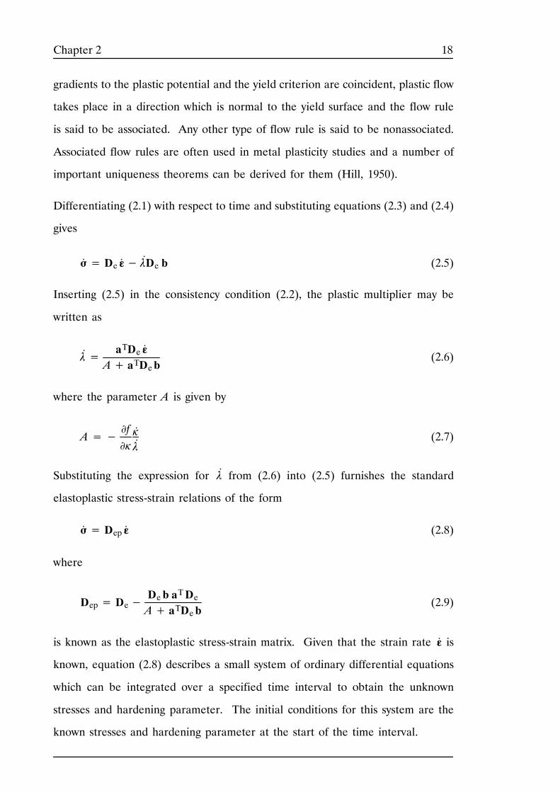
Differentiating (2.1) with respect to time and substituting equations (2.3) and (2.4)
gives
σ. = De ε
. − λ.De b (2.5)
Inserting (2.5) in the consistency condition (2.2), the plastic multiplier may be
written as
λ.=
aTDe ε.
A+ aTDeb(2.6)
where the parameter A is given by
A=−∂f∂ÀÀ.
λ. (2.7)
Substituting the expression for λ.from (2.6) into (2.5) furnishes the standard
elastoplastic stress-strain relations of the form
σ. = Dep ε
. (2.8)
where
Dep= De−De b aTDeA+ aTDeb
(2.9)
is known as the elastoplastic stress-strain matrix. Given that the strain rate ε. is
known, equation (2.8) describes a small system of ordinary differential equations
which can be integrated over a specified time interval to obtain the unknown
stresses and hardening parameter. The initial conditions for this system are the
known stresses and hardening parameter at the start of the time interval.
19Chapter 2
The elastoplastic stress-strain matrix (2.9) may also be expressed as a combination
of elastic and plastic components according to
Dep= De−Dp (2.10)
In this equation, De is the usual elastic stress-strain matrix and
Dp=Deb aTDeA+ aTDeb
represents the plastic contribution to the elastoplastic stress strain matrix. This
decomposition of the elastoplastic stress-strain matrix provides substantial
computational efficiencies, and will be discussed in a later Chapter.
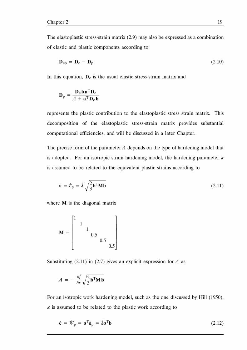
The precise form of the parameter A depends on the type of hardening model that
is adopted. For an isotropic strain hardening model, the hardening parameter À
is assumed to be related to the equivalent plastic strains according to
À. = ε
.p= λ
. 23bTMb (2.11)
where M is the diagonal matrix
M=⎪⎪⎪⎪⎪
⎡
⎣
1110.50.50.5
⎪⎪⎪⎪⎪
⎤
⎦
Substituting (2.11) in (2.7) gives an explicit expression for A as
A=−∂f∂À
23bTMb
For an isotropic work hardening model, such as the one discussed by Hill (1950),
À is assumed to be related to the plastic work according to
À. = W
.
p= σTε.p= λ
.σTb (2.12)
20Chapter 2
In this case, equation (2.7) gives the parameter A as
A=−∂f∂Àσ
Tb
Both of the hardening models require integration over the strain path to give the
hardening parameter. Equations (2.11) and (2.12) define the ordinary differential
equations that need to be integrated over each specified time interval to give À.
2.3 GOVERNING LOAD-DEFLECTION EQUATIONS
Consider a body with volume V and surface area S. The stresses within the body
must be in equilibrium and this condition provides a starting point for formulating
the governing load-deflection equations in finite element analysis. The equations
of equilibrium for a three dimensional solid are
∂σx∂x +
∂τxy∂y +
∂τxz∂z + bx= 0
∂σy∂y +
∂τyx∂x +
∂τyz∂z + by= 0 (2.13)
∂σz∂z +
∂τzx∂x +
∂τzy∂y + bz= 0
where bx, by and bz are components of the body force in the x-, y- and z-directions
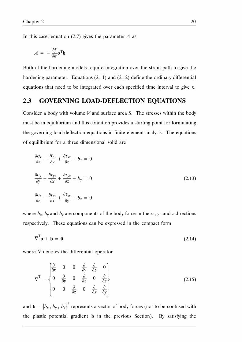
respectively. These equations can be expressed in the compact form
∇Tσ+ b= 0 (2.14)
where ∇ denotes the differential operator
∇T=⎪
⎪⎨
⎧
⎩
∂∂x
0
0
0
∂∂y
0
0
0
∂∂z
∂∂y∂∂x
0
∂∂z
0
∂∂x
0
∂∂z∂∂y⎪
⎪⎬
⎫
⎭
(2.15)
and b= bx , by , bzTrepresents a vector of body forces (not to be confused with
the plastic potential gradient b in the previous Section). By satisfying the
21Chapter 2
equilibrium equations throughout the body, together with any associated boundary
conditions, the stresses, strains, and deformations within the body can be
determined. One technique for expressing the equilibrium equations in an average
sense is the method of weighted residuals. When applied to equation (2.14), this
method requires that
W= V
wT∇Tσ+ bdV= 0
where w= wx , wy , wzTis a vector of arbitrary weighting functions with
components in the x- , y- and z-directions. Integrating the above equation by parts
using the Green-Gauss theorem gives the so-called weak form of the equilibrium
equations as
V
(∇w)Tσ dV−V
wTb dV−S
wTtdS= 0 (2.16)
where t= tx , ty , tzTis a vector of surface tractions which act over the boundary
surface S. These tractions must satisfy the boundary conditions
txtytz
===
σx nxτxy nxτxz nx
+++
τxy nyσy nyτyz ny
+++
τxz nzτyz nzσz nz
in which nx, ny and nz are direction cosines of the unit normal to the surface S.
An approximate form of equation (2.16) can be obtained by the application of the
finite element method. This involves dividing the body into a number of
sub-domains, known as elements, over which the displacements are approximated
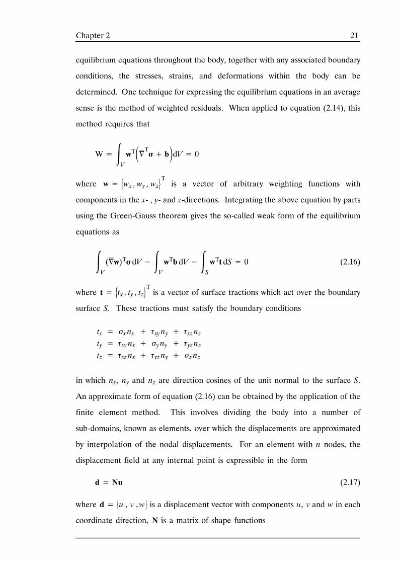
by interpolation of the nodal displacements. For an element with n nodes, the
displacement field at any internal point is expressible in the form
d= Nu (2.17)
where d= u , v ,w is a displacement vector with components u, v and w in each
coordinate direction, N is a matrix of shape functions
22Chapter 2
N=⎪⎡
⎣
N100
0N10
00N1
N200
0N20
00N2
...
...
...
Nn00
0Nn0
00Nn⎪⎤
⎦(2.18)
and u is a vector of element nodal displacements
u= u1, v1, w1, u2, v2, w2, ... un, vn, wnT
(2.19)
The corresponding internal strains are given by differentiating (2.17) to give
ε= Bu (2.20)
where B is the element strain-displacement matrix
B= ∇N=
⎪⎪⎪⎪⎪⎪⎪⎪⎪⎪⎪⎪⎪⎪⎪⎪
⎡
⎣
∂N1∂x
0
0
∂N1∂y∂N1∂z
0
0
∂N1∂y
0
∂N1∂x
0
∂N1∂z
0
0
∂N1∂z
0
∂N1∂x∂N1∂y
...
...
...
...
...
...
∂Nn∂x
0
0
∂Nn∂y∂Nn∂z
0
0
∂Nn∂y
0
∂Nn∂x
0
∂Nn∂z
0
0
∂Nn∂z
0
∂Nn∂x∂Nn∂y
⎪⎪⎪⎪⎪⎪⎪⎪⎪⎪⎪⎪⎪⎪⎪⎪
⎤
⎦
Having defined the functional form of the displacements, the weighting functions
may be chosen as
w= δd= N δu (2.21)
where δu is a vector of arbitrary nodal displacements for an element. Using this
weighting scheme, the method of weighted residuals reduces to the classical
approach of Galerkin (1915). Substituting the weighting functions (2.21) into
(2.16), integrating over the element volume, V e, and surface area, Se, and
collecting terms furnishes
δuT⎪⎧⎩VeBTσ dV−
SeNTt dS−
VeNTb dV⎪⎫⎭
= 0 (2.22)
23Chapter 2
Since the displacements δu are arbitrary, it follows that
VeBTσ dV−
SeNTt dS−
VeNTb dV= 0 (2.23)
for (2.22) to be true in the general case. These equations, which govern the
behaviour of each finite element, are applicable to any constitutive relationship.
Since they describe the overall equilibrium conditions, they are often written in
the form
f ext− f int= 0 (2.24)
where the external forces are given by
f ext= VeNTb dV+
SeNTt dS (2.25)
and the internal forces are defined as
f int= VeBTσ dV (2.26)
The vector f ext comprises the nodal forces exerted on the element due to the
applied loading, while the vector f int comprises the nodal forces which are
supported by the internal stresses in the element.
For nonlinear problems it is necessary to develop an incremental or rate form of
equation (2.24). This may be obtained by differentiating equation (2.24) with
respect to time t and using the chain rule to give
dfdt
ext− dfdu
intdudt= 0 (2.27)
where the derivative of f int with respect to u is the Jacobian matrix
24Chapter 2
dfdu
int=
⎪⎪⎪⎪⎪⎪⎪⎪⎪⎪⎪
⎡
⎣
∂f int1∂u1
∂f int2∂u1⋮
∂f intn∂u1
∂f int1∂u2
∂f int2∂u2⋮
∂f intn∂u2
...
...
...
∂f int1∂un
∂f int2∂un⋮
∂f intn∂un
⎪⎪⎪⎪⎪⎪⎪⎪⎪⎪⎪
⎤
⎦
Now, from equation (2.25), it follows that
dfdu
int=
VeBT dσdudV=
VeBT dσdεdεdudV (2.28)
Neglecting terms involving second derivatives of the yield function with respect to
the stresses, the derivative of σ with respect to ε is
dσdε= Dep (2.29)
where Dep is the elastoplastic stress-strain matrix defined in (2.9). Similarly, the
derivative of the strains with respect to the nodal deflections is obtained by
differentiating the strain-displacement relations (2.20) to give
dεdu= B (2.30)
Substituting (2.29) and (2.30) in (2.28) leads to the definition of the elastoplastic
tangent stiffness matrix, kep, according to
dfdu
int=
VeBTDepB dV= kep (2.31)
Finally, combining equations (2.31) and (2.27) and rearranging gives
dudt= k–1ep dfdt
ext
or
25Chapter 2
u. = k–1ep f. ext (2.32)
where the superior dot again denotes a derivative with respect to time. The
relations (2.32) define a system of ordinary differential equations which govern the
load-deformation behaviour of a single elastoplastic element. Adding these
element contributions together in the usual way gives a system of ordinary
differential equations of the form
U.= K–1ep F
. ext (2.33)
where
Kep= elements
kep= elements
VeBTDepB dV
and
F. ext=
elements
f. ext=
elements
VeNTb
.dV+
elements
SeNT t
.dS
are, respectively, the global elastoplastic stiffness matrix and the global external
force rate vector. The relations (2.33) describe, in rate form, the global
load-displacement behaviour of a mesh of elastoplastic finite elements. The initial
conditions for these ordinary differential equations are the displacements, stresses
and hardening parameters which are known at the start of each time interval.
2.4 YIELD CRITERIA
The Mohr-Coulomb yield criterion, with either an associated or nonassociated
flow rule, is used widely in geotechnical analysis. Although more sophisticated
constitutive laws are available for predicting the behaviour of real soil, this simple
model has the important advantage that all of its parameters have direct physical
meanings and can be measured using conventional tests. Although it predicts an
excessive amount of dilation upon plastic shearing, the Mohr-Coulomb yield
26Chapter 2
criterion is traditionally employed with an associated flow rule. This type of model
has been assumed in many limit equilibrium and classical plasticity solutions
which, apart from being valuable in their own right, are especially useful for
validating finite element codes.
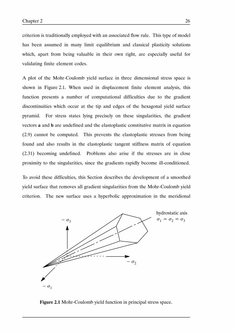
A plot of the Mohr-Coulomb yield surface in three dimensional stress space is
shown in Figure 2.1. When used in displacement finite element analysis, this
function presents a number of computational difficulties due to the gradient
discontinuities which occur at the tip and edges of the hexagonal yield surface
pyramid. For stress states lying precisely on these singularities, the gradient
vectors a and b are undefined and the elastoplastic constitutive matrix in equation
(2.9) cannot be computed. This prevents the elastoplastic stresses from being
found and also results in the elastoplastic tangent stiffness matrix of equation
(2.31) becoming undefined. Problems also arise if the stresses are in close
proximity to the singularities, since the gradients rapidly become ill-conditioned.
To avoid these difficulties, this Section describes the development of a smoothed
yield surface that removes all gradient singularities from the Mohr-Coulomb yield
criterion. The new surface uses a hyperbolic approximation in the meridional
Figure 2.1Mohr-Coulomb yield function in principal stress space.
− σ1
− σ3
− σ2
σ1= σ2= σ3hydrostatic axis
27Chapter 2
plane to eliminate the tip singularity and a trigonometric rounding in the
octahedral plane to eliminate the edge singularities. It is both continuous and
differentiable for all stress states, and can be fitted to the Mohr-Coulomb yield
surface by adjusting two parameters.
2.4.1 Rounded Mohr-Coulomb Yield Function
Defining tensile stresses as positive, the Mohr-Coulomb yield function may be
written as
f= (σ1− σ3)+ (σ1+ σ3) sinφ− 2c cosφ= 0 (2.34)
where the principal stresses are ordered so that σ1≥ σ2≥ σ3 and c and φ denote,
respectively, the cohesion and friction angle of the soil.
For computational convenience, the Mohr-Coulomb criterion can be expressed in
terms of the three stress invariants originally proposed by Nayak and Zienkiewicz
(1972b). These quantities are written as (σm, σ, θ) and are defined by
σm= 13 (σx+ σy+ σz)
σ= 12s2x+ s2y + s2z + τ2xy+ τ2yz+ τ2zx
θ= 13 sin–1− 3 32 J3
σ 3 , (− 30˚≤ θ≤ 30˚)
where
J3= sx sy sz+ 2 τxy τyz τzx− sx τ2yz− sy τ2xz− sz τ2xy
and
sx= σx− σm , sy= σy− σm , sz= σz− σm
In terms of these invariants, the principal stresses are given by
28Chapter 2
σ1=23σ sin(θ+ 120˚)+ σm (2.35)
σ2=23σ sin(θ)+ σm
σ3=23σ sin(θ− 120˚)+ σm (2.36)
Substituting (2.35) and (2.36) in (2.34), the Mohr-Coulomb yield criterion may be
expressed in the equivalent form
f = σm sinφ+ σ K(θ)− c cosφ = 0 (2.37)
where the function K is
K(θ)= cos θ− 13sinφ sin θ (2.38)
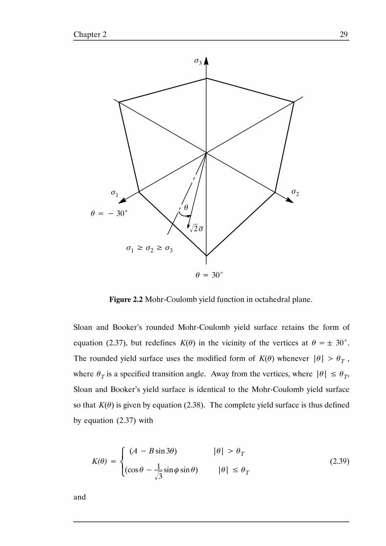
In the octahedral plane, defined by σm = constant, the shape of the yield function
is defined by the relationship between σ and θ. When viewed in this plane, the
Mohr-Coulomb surface has sharp vertices (and hence gradient discontinuities) at
θ= 30˚ as shown in Figure 2.2. It is necessary to permit the gradients to be
computed at these stress states since they are often encountered in finite element
analysis. Various techniques for dealing with these corners have been discussed
by Zienkiewicz and Pande (1977), Owen and Hinton (1980) and Sloan and Booker
(1986). Of these methods, the Sloan and Booker procedure has the advantage that
it uses a trigonometric rounding only in the vicinity of the vertices and thus models
the Mohr-Coulomb yield surface very closely. Because the modified yield surface
is internal to the Mohr-Coulomb criterion, this approximation also ensures that
the strength is modelled conservatively. Except for tensile hydrostatic stress states,
the Sloan and Booker (1986) surface is continuous and differentiable for all stress
states, and can be fitted to the Mohr-Coulomb surface as closely as desired by
adjusting a single parameter.
29Chapter 2
Figure 2.2Mohr-Coulomb yield function in octahedral plane.
σ1
σ3
σ2
σ1≥ σ2≥ σ3
θ= 30˚
θ=− 30˚
2 σ
θ
Sloan and Booker’s rounded Mohr-Coulomb yield surface retains the form of
equation (2.37), but redefines K(θ) in the vicinity of the vertices at θ= 30˚.
The rounded yield surface uses the modified form of K(θ) whenever |θ|> θT ,
where θT is a specified transition angle. Away from the vertices, where |θ|≤ θT,
Sloan and Booker’s yield surface is identical to the Mohr-Coulomb yield surface
so that K(θ) is given by equation (2.38). The complete yield surface is thus defined
by equation (2.37) with
K(θ)=⎨⎧⎩
(A− B sin 3θ) |θ|> θT
(cos θ− 13sinφ sin θ) |θ|≤ θT
(2.39)
and
30Chapter 2
A= 13 cos θT3+ tan θT tan 3θT+ 13 sign(θ)(tan 3θT− 3 tan θT) sinφ (2.40)
B= 13 cos 3θTsign(θ) sin θT+ 13 sinφ cos θT (2.41)
sign(θ)= + 1 for θ≥ 0˚− 1 for θ< 0˚
The value of the transition angle lies within the range 0≤ θT≤ 30˚, with larger
values giving better fits to the Mohr-Coulomb cross-section in the octahedral
plane. In practice, θT should not be too near 30˚to avoid ill-conditioning of the
approximation, and a typical value is 25˚. Once the transition angle is specified,
the coefficients A and B may be computed efficiently by evaluating all of the
constant terms in equations (2.40) and (2.41) respectively. A π-plane plot of Sloan
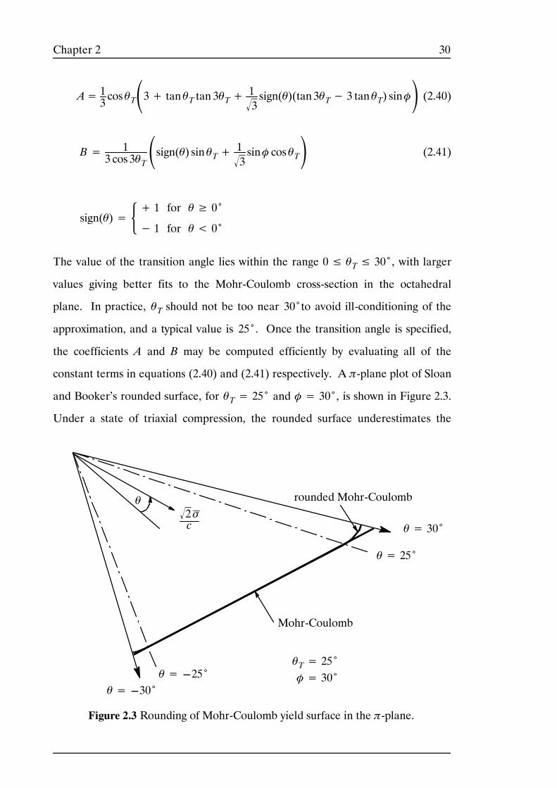
and Booker’s rounded surface, for θT= 25˚ and φ= 30˚, is shown in Figure 2.3.
Under a state of triaxial compression, the rounded surface underestimates the
θ= ---25˚
θ= 30˚
θ= ---30˚
θT= 25˚φ= 30˚
θ= 25˚
θ
Mohr-Coulomb
2 σc
Figure 2.3 Rounding of Mohr-Coulomb yield surface in the π-plane.
rounded Mohr-Coulomb
31Chapter 2
Mohr-Coulomb value for σ∕c by approximately 4.4 per cent. For a state of triaxial
extension, this difference is reduced to roughly 1.1 per cent.
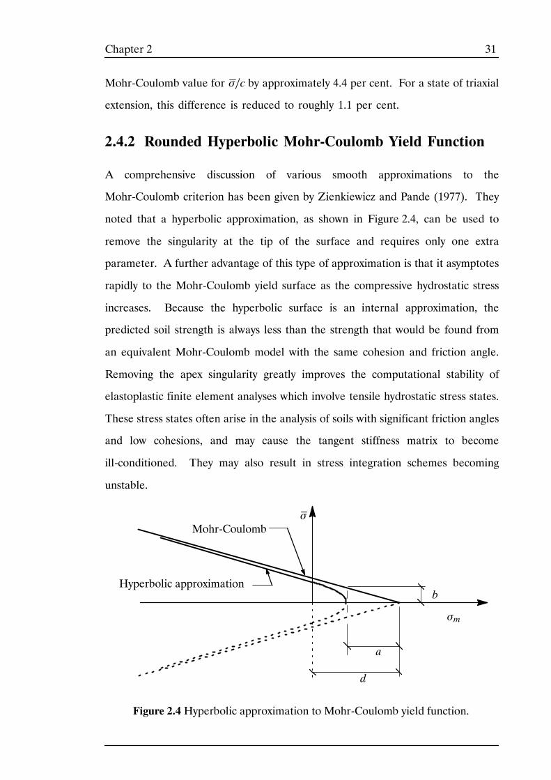
2.4.2 Rounded Hyperbolic Mohr-Coulomb Yield Function
A comprehensive discussion of various smooth approximations to the
Mohr-Coulomb criterion has been given by Zienkiewicz and Pande (1977). They
noted that a hyperbolic approximation, as shown in Figure 2.4, can be used to
remove the singularity at the tip of the surface and requires only one extra
parameter. A further advantage of this type of approximation is that it asymptotes
rapidly to the Mohr-Coulomb yield surface as the compressive hydrostatic stress
increases. Because the hyperbolic surface is an internal approximation, the
predicted soil strength is always less than the strength that would be found from
an equivalent Mohr-Coulomb model with the same cohesion and friction angle.
Removing the apex singularity greatly improves the computational stability of
elastoplastic finite element analyses which involve tensile hydrostatic stress states.
These stress states often arise in the analysis of soils with significant friction angles
and low cohesions, and may cause the tangent stiffness matrix to become
ill-conditioned. They may also result in stress integration schemes becoming
unstable.
σ
σm
a
b
d
Hyperbolic approximation
Mohr-Coulomb
Figure 2.4 Hyperbolic approximation to Mohr-Coulomb yield function.
32Chapter 2
The relationship between σ and σm , for a constant θ, defines a meridional section
of the yield surface. For the Mohr-Coulomb criterion, this relationship can be
represented as a straight line in (σm , σ ) space as shown in Figure 2.4. The point
where the line cuts the σm-axis corresponds to the tip of the hexagonal
Mohr-Coulomb pyramid, and it is here that the gradient of the yield surface is
undefined.
The equation of the straight line defining the Mohr-Coulomb yield function in the
meridional plane can be determined directly from equation (2.37) as
σ = 1K(θ)
c cosφ− σm sinφ
The slope of this line is − sinφ∕K(θ) and it intercepts the σm-axis at
σm= c cotφ. Following Zienkiewicz and Pande (1977), a close approximation to
the straight line which defines the Mohr-Coulomb yield surface can be obtained
using an asymptotic hyperbola. The general equation of such a hyperbola, in
(σm , σ ) space, is
(σm− d )2
a2− σ
2
b2= 1 (2.42)
where a, b and d are the distances defined in Figure 2.4. The upper asymptote
to this hyperbola has slope − b∕a and crosses the σm-axis at σm= d. Equating
the slope and intercept of the Mohr-Coulomb surface to the slope and intercept
of the hyperbolic asymptote yields the two relations
ba=
sinφK(θ)
, d= c cotφ
Substituting these expressions into equation (2.42) gives the yield surface
f = σm+ σ 2K2(θ)+ a2 sin2φ − c cosφ= 0 (2.43)
where the negative branch of the hyperbola has been chosen. This function can
be made to model the Mohr-Coulomb yield function as closely as desired by
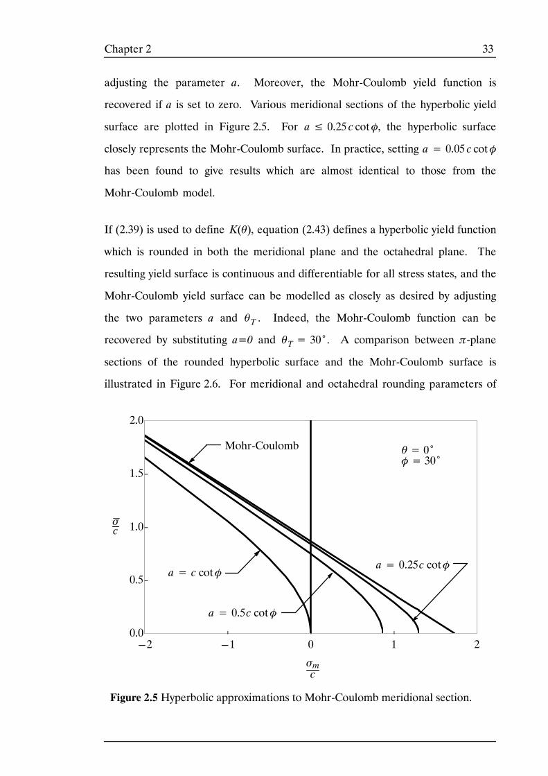
33Chapter 2
adjusting the parameter a. Moreover, the Mohr-Coulomb yield function is
recovered if a is set to zero. Various meridional sections of the hyperbolic yield
surface are plotted in Figure 2.5. For a≤ 0.25 c cotφ, the hyperbolic surface
closely represents the Mohr-Coulomb surface. In practice, setting a= 0.05 c cotφ
has been found to give results which are almost identical to those from the
Mohr-Coulomb model.
If (2.39) is used to define K(θ), equation (2.43) defines a hyperbolic yield function
which is rounded in both the meridional plane and the octahedral plane. The
resulting yield surface is continuous and differentiable for all stress states, and the
Mohr-Coulomb yield surface can be modelled as closely as desired by adjusting
the two parameters a and θT . Indeed, the Mohr-Coulomb function can be
recovered by substituting a=0 and θT= 30˚. A comparison between π-plane
sections of the rounded hyperbolic surface and the Mohr-Coulomb surface is
illustrated in Figure 2.6. For meridional and octahedral rounding parameters of
0.0
0.5
1.0
1.5
2.0
---2 ---1 0 1 2
a= 0.5c cotφ
a= 0.25c cotφ
σc
a= c cotφ
Mohr-Coulomb θ= 0˚φ= 30˚
Figure 2.5 Hyperbolic approximations to Mohr-Coulomb meridional section.
σmc
34Chapter 2
θ= ---25˚
a= 0.25c cotφ
θ= 30˚
θ= ---30˚
θT= 25˚φ= 30˚
θ= 25˚
a= 0.5c cotφ
θ
a= 0 (Mohr-Coulomb)
2 σc
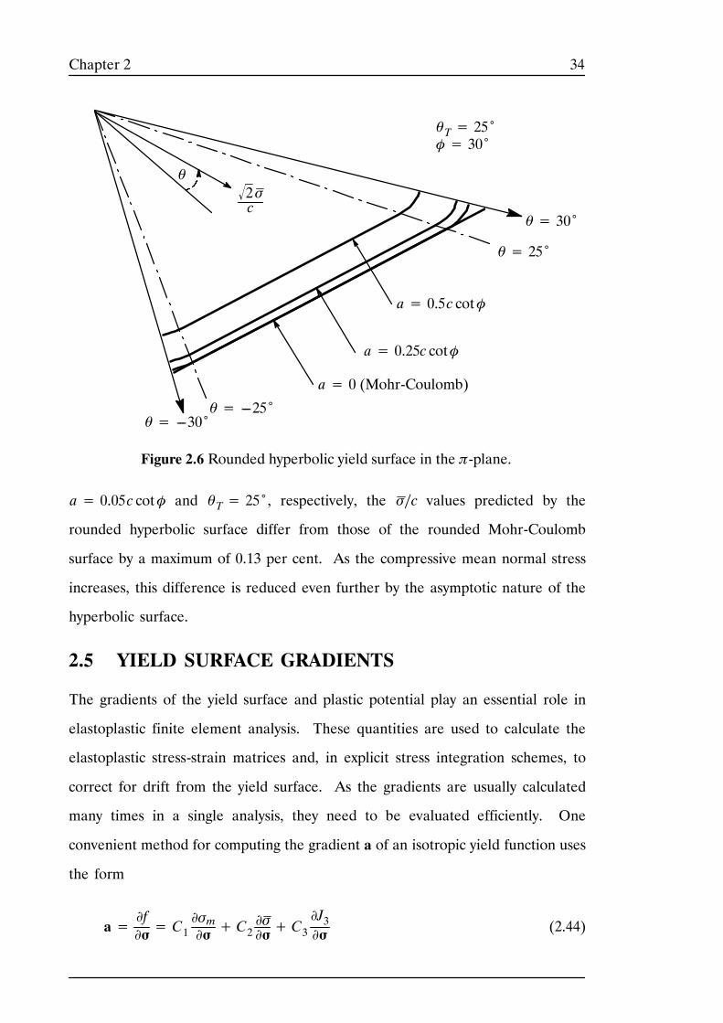
Figure 2.6 Rounded hyperbolic yield surface in the π-plane.
a= 0.05c cotφ and θT= 25˚, respectively, the σ∕c values predicted by the
rounded hyperbolic surface differ from those of the rounded Mohr-Coulomb
surface by a maximum of 0.13 per cent. As the compressive mean normal stress
increases, this difference is reduced even further by the asymptotic nature of the
hyperbolic surface.
2.5 YIELD SURFACE GRADIENTS
The gradients of the yield surface and plastic potential play an essential role in
elastoplastic finite element analysis. These quantities are used to calculate the
elastoplastic stress-strain matrices and, in explicit stress integration schemes, to
correct for drift from the yield surface. As the gradients are usually calculated
many times in a single analysis, they need to be evaluated efficiently. One
convenient method for computing the gradient a of an isotropic yield function uses
the form
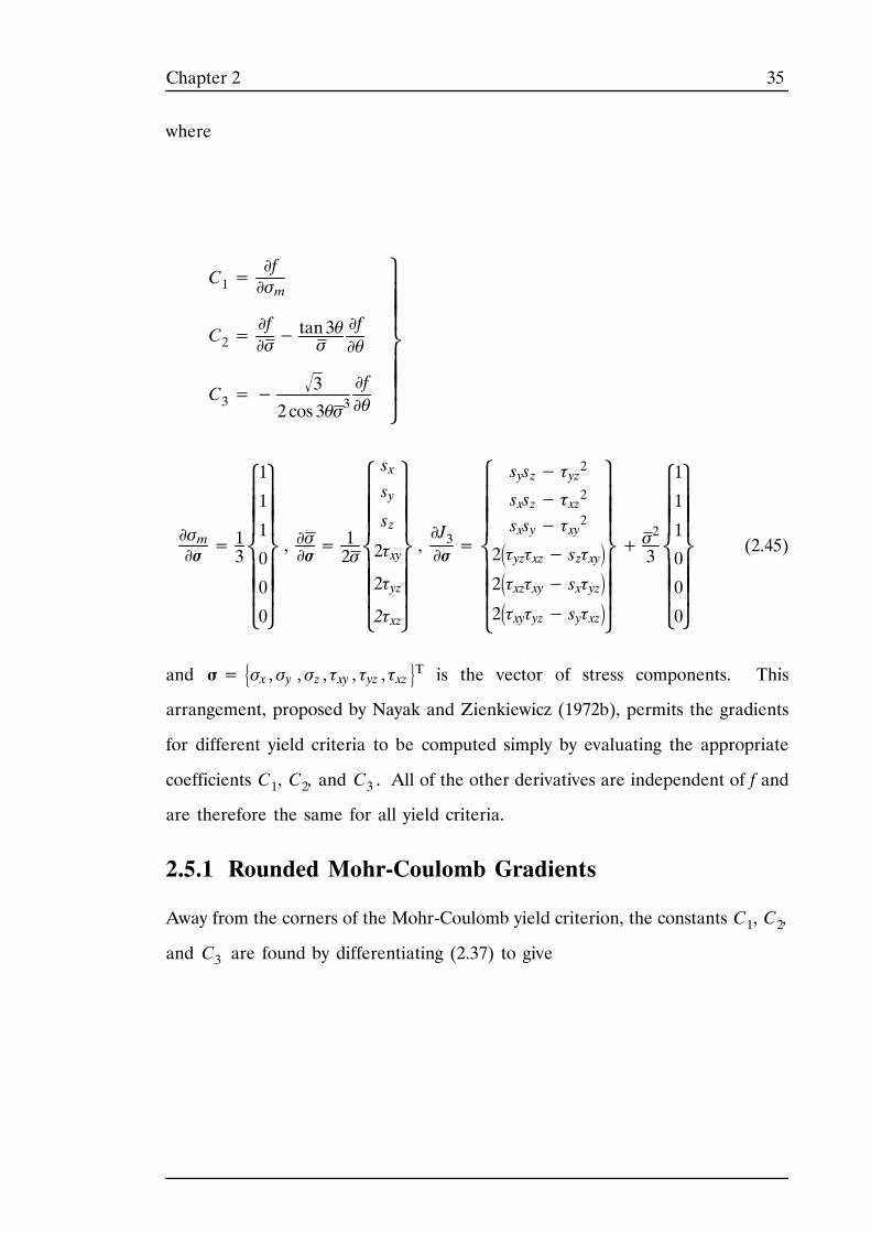
a=∂f∂σ= C1
∂σm∂σ + C2
∂σ∂σ+ C3
∂J3∂σ (2.44)
35Chapter 2
where
C1=∂f∂σm
C2=∂f∂σ−
tan 3θσ∂f∂θ
C3=−3
2 cos 3θσ3∂f∂θ
⎪⎪⎪
⎪⎪⎪⎬
⎫
⎭
∂σm∂σ =
13⎪⎪⎪
⎪⎪⎪⎨
⎧
⎩
1
1
1
0
0
0
⎪⎪⎪
⎪⎪⎪⎬
⎫
⎭
, ∂σ∂σ=12σ⎪⎪⎪
⎪⎪⎪⎨
⎧
⎩
sxsysz
2τxy
2τyz
2τxz
⎪⎪⎪
⎪⎪⎪⎬
⎫
⎭
,∂J3∂σ =⎪⎪⎪
⎪⎪⎪⎨
⎧
⎩
sysz− τyz2
sxsz− τxz2
sxsy− τxy2
2τyzτxz− szτxy2τxzτxy− sxτyz2τxyτyz− syτxz
⎪⎪⎪
⎪⎪⎪⎬
⎫
⎭
+ σ2
3 ⎪⎪⎪
⎪⎪⎪⎨
⎧
⎩
1
1
1
0
0
0
⎪⎪⎪
⎪⎪⎪⎬
⎫
⎭
(2.45)
and σ= σx , σy , σz , τxy , τyz , τxz T is the vector of stress components. This
arrangement, proposed by Nayak and Zienkiewicz (1972b), permits the gradients
for different yield criteria to be computed simply by evaluating the appropriate
coefficients C1, C2, and C3 . All of the other derivatives are independent of f and
are therefore the same for all yield criteria.
2.5.1 Rounded Mohr-Coulomb Gradients
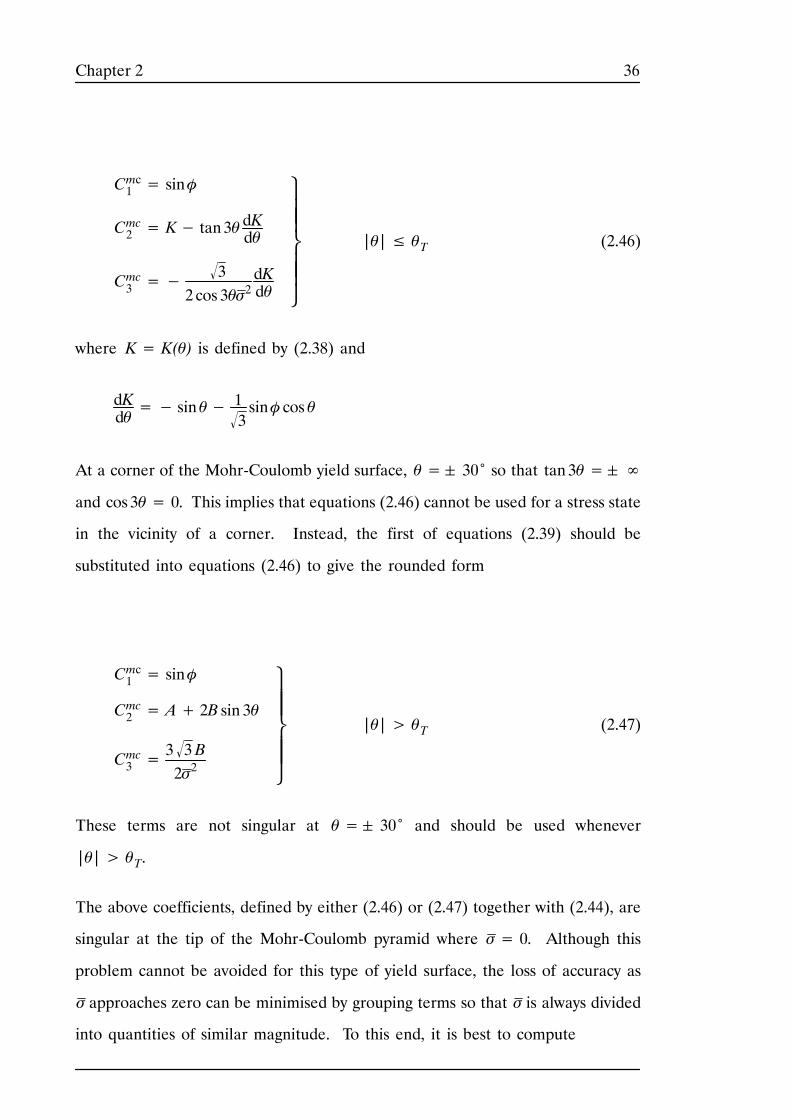
Away from the corners of the Mohr-Coulomb yield criterion, the constants C1, C2,
and C3 are found by differentiating (2.37) to give
36Chapter 2
Cmc1 = sinφ
Cmc2 = K− tan 3θdKdθ
Cmc3 =−3
2 cos 3θσ2dKdθ
⎪⎪
⎪⎪⎬
⎫
⎭
|θ|≤ θT (2.46)
where K= K(θ) is defined by (2.38) and
dKdθ=− sin θ− 1
3sinφ cos θ
At a corner of the Mohr-Coulomb yield surface, θ= 30˚ so that tan 3θ=∞
and cos 3θ= 0. This implies that equations (2.46) cannot be used for a stress state
in the vicinity of a corner. Instead, the first of equations (2.39) should be
substituted into equations (2.46) to give the rounded form
Cmc1 = sinφ
Cmc2 = A+ 2B sin 3θ
Cmc3 =3 3 B2σ2
⎪⎪
⎪⎪⎬
⎫
⎭
|θ|> θT (2.47)
These terms are not singular at θ= 30˚ and should be used whenever
|θ|> θT.
The above coefficients, defined by either (2.46) or (2.47) together with (2.44), are
singular at the tip of the Mohr-Coulomb pyramid where σ= 0. Although this
problem cannot be avoided for this type of yield surface, the loss of accuracy as
σ approaches zero can be minimised by grouping terms so that σ is always divided
into quantities of similar magnitude. To this end, it is best to compute
37Chapter 2
Cmc3 = Cmc3 σ
2
and then evaluate the last term in (2.44) using
C3∂J3∂σ = C
mc3
⎪⎪⎪⎪⎪⎪⎪⎪⎪
⎧
⎩
1σ2⎪⎪⎪
⎪⎪⎪⎨
⎧
⎩
sysz− τyz2
sxsz− τxz2
sxsy− τxy2
2τyzτxz− szτxy2τxzτxy− sxτyz2τxyτyz− syτxz
⎪⎪⎪
⎪⎪⎪⎬
⎫
⎭
+ 13⎪⎪⎪
⎪⎪⎪⎨
⎧
⎩
1
1
1
0
0
0
⎪⎪⎪
⎪⎪⎪⎬
⎫
⎭
⎪⎪⎪⎪⎪⎪⎪⎪⎪
⎫
⎭
This procedure can be used for all values of σ and θ.
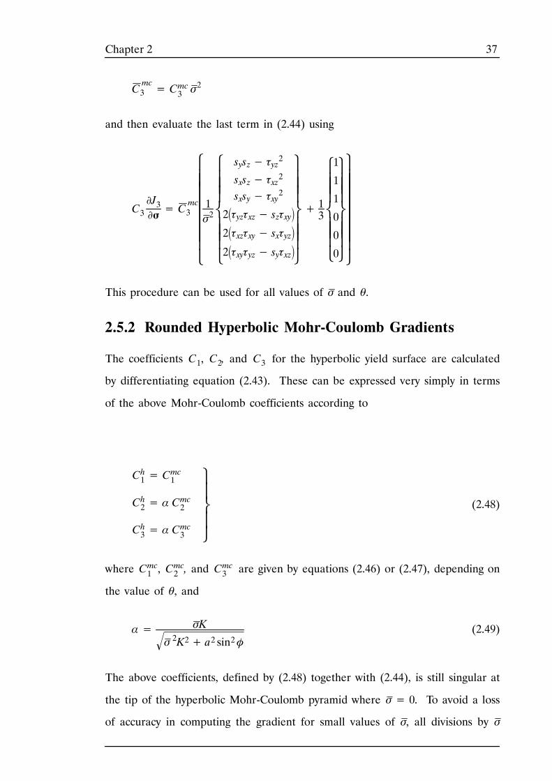
2.5.2 Rounded Hyperbolic Mohr-Coulomb Gradients
The coefficients C1, C2, and C3 for the hyperbolic yield surface are calculated
by differentiating equation (2.43). These can be expressed very simply in terms
of the above Mohr-Coulomb coefficients according to
Ch1 = Cmc1
Ch2 = α Cmc2
Ch3 = α Cmc3
⎪
⎪⎬
⎫
⎭
(2.48)
where Cmc1 , Cmc2 , and C
mc3 are given by equations (2.46) or (2.47), depending on
the value of θ, and
α= σK
σ 2K2+ a2 sin2 φ (2.49)
The above coefficients, defined by (2.48) together with (2.44), is still singular at
the tip of the hyperbolic Mohr-Coulomb pyramid where σ= 0. To avoid a loss
of accuracy in computing the gradient for small values of σ, all divisions by σ
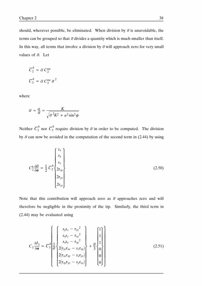
38Chapter 2
should, wherever possible, be eliminated. When division by σ is unavoidable, the
terms can be grouped so that σ divides a quantity which is much smaller than itself.
In this way, all terms that involve a division by σ will approach zero for very small
values of σ. Let
Ch2 = α Cmc2
Ch3 = α Cmc3 σ
2
where
α= ασ=K
σ 2K2+ a2 sin2φ
Neither Ch2 nor C
h3 require division by σ in order to be computed. The division
by σ can now be avoided in the computation of the second term in (2.44) by using
Ch2∂σ∂σ=
12 C
h2
⎪⎪⎪
⎪⎪⎪⎨
⎧
⎩
sxsysz
2τxy
2τyz
2τxz
⎪⎪⎪
⎪⎪⎪⎬
⎫
⎭
(2.50)
Note that this contribution will approach zero as σ approaches zero and will
therefore be negligible in the proximity of the tip. Similarly, the third term in
(2.44) may be evaluated using
C3∂J3∂σ = C
h3
⎪⎪⎪⎪⎪⎪⎪⎪⎪
⎧
⎩
1σ⎪⎪⎪
⎪⎪⎪⎨
⎧
⎩
sysz− τyz2
sxsz− τxz2
sxsy− τxy2
2τyzτxz− szτxy2τxzτxy− sxτyz2τxyτyz− syτxz
⎪⎪⎪
⎪⎪⎪⎬
⎫
⎭
+ σ3⎪⎪⎪
⎪⎪⎪⎨
⎧
⎩
1
1
1
0
0
0
⎪⎪⎪
⎪⎪⎪⎬
⎫
⎭
⎪⎪⎪⎪⎪⎪⎪⎪⎪
⎫
⎭
(2.51)
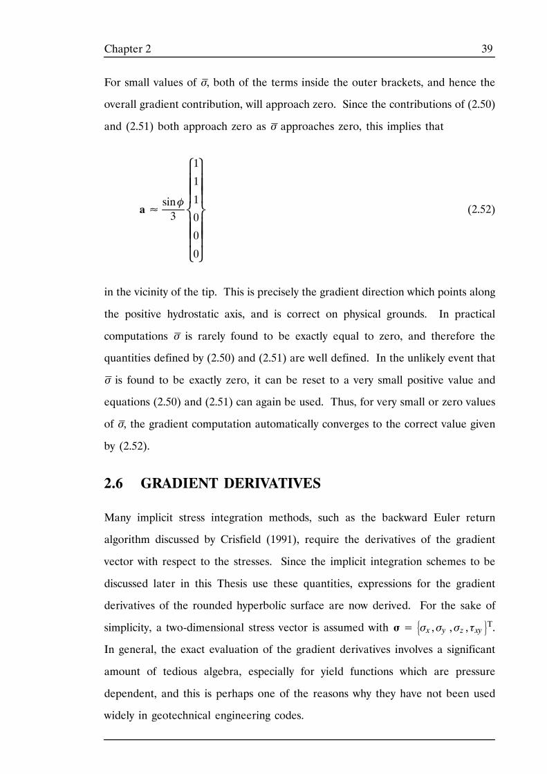
39Chapter 2
For small values of σ, both of the terms inside the outer brackets, and hence the
overall gradient contribution, will approach zero. Since the contributions of (2.50)
and (2.51) both approach zero as σ approaches zero, this implies that
a≈sinφ3 ⎪⎪⎪
⎪⎪⎪⎨
⎧
⎩
1
1
1
0
0
0
⎪⎪⎪
⎪⎪⎪⎬
⎫
⎭
(2.52)
in the vicinity of the tip. This is precisely the gradient direction which points along
the positive hydrostatic axis, and is correct on physical grounds. In practical
computations σ is rarely found to be exactly equal to zero, and therefore the
quantities defined by (2.50) and (2.51) are well defined. In the unlikely event that
σ is found to be exactly zero, it can be reset to a very small positive value and
equations (2.50) and (2.51) can again be used. Thus, for very small or zero values
of σ, the gradient computation automatically converges to the correct value given
by (2.52).
2.6 GRADIENT DERIVATIVES
Many implicit stress integration methods, such as the backward Euler return
algorithm discussed by Crisfield (1991), require the derivatives of the gradient
vector with respect to the stresses. Since the implicit integration schemes to be
discussed later in this Thesis use these quantities, expressions for the gradient
derivatives of the rounded hyperbolic surface are now derived. For the sake of
simplicity, a two-dimensional stress vector is assumed with σ= σx , σy , σz , τxy T.
In general, the exact evaluation of the gradient derivatives involves a significant
amount of tedious algebra, especially for yield functions which are pressure
dependent, and this is perhaps one of the reasons why they have not been used
widely in geotechnical engineering codes.
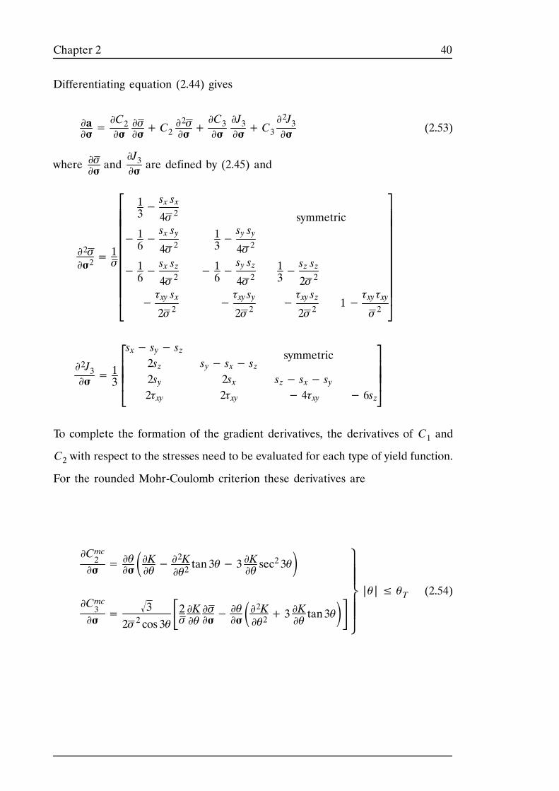
40Chapter 2
Differentiating equation (2.44) gives
∂a∂σ=
∂C2∂σ∂σ∂σ+ C2
∂2σ∂σ +
∂C3∂σ∂J3∂σ + C3
∂2J3∂σ (2.53)
where ∂σ∂σ and∂J3∂σ are defined by (2.45) and
symmetric
∂2σ∂σ2= 1σ
⎪⎪⎪⎪⎪⎪⎪⎪⎪⎪⎪
⎡
⎣
13−sx sx4σ 2
− 16−sx sy4σ 2
− 16−sx sz4σ 2
−τxy sx2σ 2
13−sy sy4σ 2
− 16−sy sz4σ 2
−τxy sy2σ 2
13−sz sz2σ 2
−τxy sz2σ 2
1−τxy τxy
σ 2
⎪⎪⎪⎪⎪⎪⎪⎪⎪⎪⎪
⎤
⎦
symmetric∂2J3∂σ =
13⎪⎪⎪
⎡
⎣
sx− sy− sz2sz2sy2τxy
sy− sx− sz2sx2τxy
sz− sx− sy− 4τxy − 6sz
⎪⎪⎪
⎤
⎦
To complete the formation of the gradient derivatives, the derivatives of C1 and
C2 with respect to the stresses need to be evaluated for each type of yield function.
For the rounded Mohr-Coulomb criterion these derivatives are
∂Cmc2∂σ =
∂θ∂σ ∂K∂θ −∂2K∂θ2 tan 3θ− 3 ∂K∂θ sec2 3θ
∂Cmc3∂σ =
3
2σ 2 cos 3θ2σ∂K∂θ∂σ∂σ−
∂θ∂σ ∂2K∂θ2 + 3 ∂K∂θ tan 3θ⎪⎪
⎪⎪⎬
⎫
⎭
|θ|≤ θT (2.54)
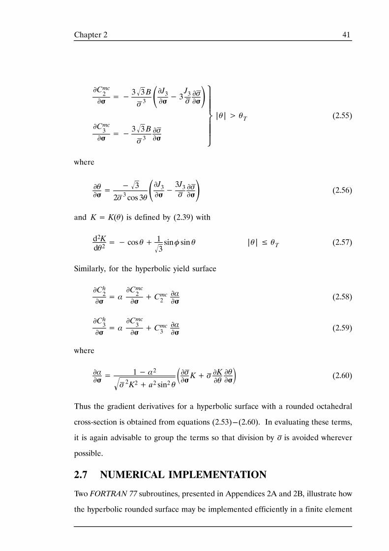
41Chapter 2
∂Cmc2∂σ =−
3 3 Bσ 3∂J3∂σ − 3 J3σ ∂σ∂σ
∂Cmc3∂σ =−
3 3 Bσ 3
∂σ∂σ
⎪⎪
⎪⎪⎬
⎫
⎭
|θ|> θT (2.55)
where
∂θ∂σ=
− 3
2σ 3 cos 3θ∂J3∂σ − 3J3σ ∂σ∂σ (2.56)
and K= K(θ) is defined by (2.39) with
d2Kdθ2=− cos θ+ 1
3sinφ sin θ |θ|≤ θT (2.57)
Similarly, for the hyperbolic yield surface
∂Ch2∂σ = α
∂Cmc2∂σ + C
mc2∂α∂σ (2.58)
∂Ch3∂σ = α
∂Cmc3∂σ + C
mc3∂α∂σ (2.59)
where
∂α∂σ =
1− α2
σ 2K2+ a2 sin2 θ ∂σ∂σK+ σ ∂K∂θ ∂θ∂σ (2.60)
Thus the gradient derivatives for a hyperbolic surface with a rounded octahedral
cross-section is obtained from equations (2.53)---(2.60). In evaluating these terms,
it is again advisable to group the terms so that division by σ is avoided wherever
possible.
2.7 NUMERICAL IMPLEMENTATION
Two FORTRAN 77 subroutines, presented in Appendices 2A and 2B, illustrate how
the hyperbolic rounded surface may be implemented efficiently in a finite element
42Chapter 2
code. The subroutines, YIELD and GRAD, return the value of the yield function
and the gradient vector, respectively, for a specified stress state. They are
applicable to two-dimensional plasticity, with either associated or nonassociated
flow, and assume that the stress vector is σ ={σx , σy , τxy , σz}T . For the case of
a nonassociated flow rule, the gradients are found by assuming that the plastic
potential is of the same form as the yield function, with the only difference being
that the dilatancy angle replaces the friction angle. As well as incorporating the
rounded hyperbolic surface, the subroutines also model the usual Mohr-Coulomb
and Tresca yield criteria (both of which are rounded in the octahedral plane).
Since this code is executed a large number of times during the course of a typical
finite element computation, considerable attention has been paid to implementing
the models with a minimum amount of arithmetic.

43Chapter 2
44 Chapter 2
APPENDICES
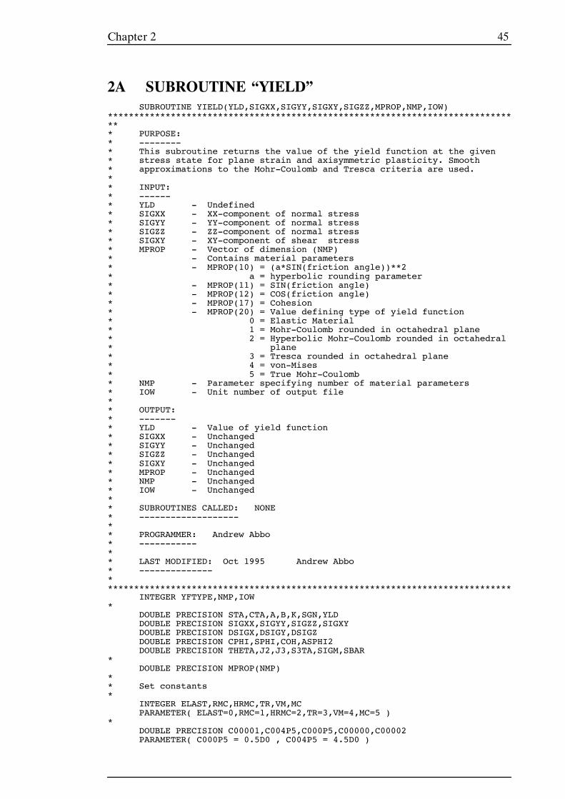
45Chapter 2
2A SUBROUTINE “YIELD”SUBROUTINE YIELD(YLD,SIGXX,SIGYY,SIGXY,SIGZZ,MPROP,NMP,IOW)
******************************************************************************** PURPOSE:* --------* This subroutine returns the value of the yield function at the given* stress state for plane strain and axisymmetric plasticity. Smooth* approximations to the Mohr-Coulomb and Tresca criteria are used.** INPUT:* ------* YLD - Undefined* SIGXX - XX-component of normal stress* SIGYY - YY-component of normal stress* SIGZZ - ZZ-component of normal stress* SIGXY - XY-component of shear stress* MPROP - Vector of dimension (NMP)* - Contains material parameters* - MPROP(10) = (a*SIN(friction angle))**2* a = hyperbolic rounding parameter* - MPROP(11) = SIN(friction angle)* - MPROP(12) = COS(friction angle)* - MPROP(17) = Cohesion* - MPROP(20) = Value defining type of yield function* 0 = Elastic Material* 1 = Mohr-Coulomb rounded in octahedral plane* 2 = Hyperbolic Mohr-Coulomb rounded in octahedral* plane* 3 = Tresca rounded in octahedral plane* 4 = von-Mises* 5 = True Mohr-Coulomb* NMP - Parameter specifying number of material parameters* IOW - Unit number of output file** OUTPUT:* -------* YLD - Value of yield function* SIGXX - Unchanged* SIGYY - Unchanged* SIGZZ - Unchanged* SIGXY - Unchanged* MPROP - Unchanged* NMP - Unchanged* IOW - Unchanged** SUBROUTINES CALLED: NONE* -------------------** PROGRAMMER: Andrew Abbo* -----------** LAST MODIFIED: Oct 1995 Andrew Abbo* --------------******************************************************************************
INTEGER YFTYPE,NMP,IOW*
DOUBLE PRECISION STA,CTA,A,B,K,SGN,YLDDOUBLE PRECISION SIGXX,SIGYY,SIGZZ,SIGXYDOUBLE PRECISION DSIGX,DSIGY,DSIGZDOUBLE PRECISION CPHI,SPHI,COH,ASPHI2DOUBLE PRECISION THETA,J2,J3,S3TA,SIGM,SBAR
*DOUBLE PRECISION MPROP(NMP)
** Set constants*
INTEGER ELAST,RMC,HRMC,TR,VM,MCPARAMETER( ELAST=0,RMC=1,HRMC=2,TR=3,VM=4,MC=5 )
*DOUBLE PRECISION C00001,C004P5,C000P5,C00000,C00002PARAMETER( C000P5 = 0.5D0 , C004P5 = 4.5D0 )
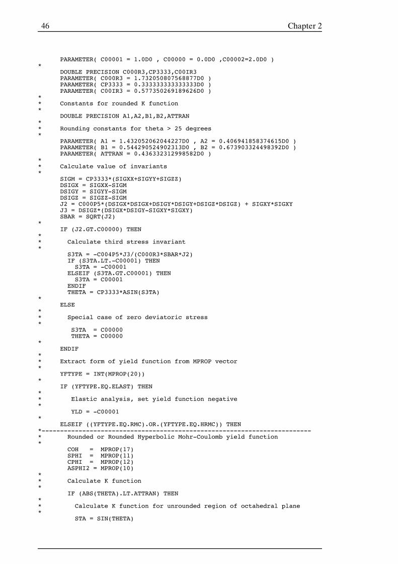
46 Chapter 2
PARAMETER( C00001 = 1.0D0 , C00000 = 0.0D0 ,C00002=2.0D0 )*
DOUBLE PRECISION C000R3,CP3333,C00IR3PARAMETER( C000R3 = 1.732050807568877D0 )PARAMETER( CP3333 = 0.333333333333333D0 )PARAMETER( C00IR3 = 0.577350269189626D0 )
** Constants for rounded K function*
DOUBLE PRECISION A1,A2,B1,B2,ATTRAN** Rounding constants for theta > 25 degrees*
PARAMETER( A1 = 1.432052062044227D0 , A2 = 0.406941858374615D0 )PARAMETER( B1 = 0.544290524902313D0 , B2 = 0.673903324498392D0 )PARAMETER( ATTRAN = 0.436332312998582D0 )
** Calculate value of invariants*
SIGM = CP3333*(SIGXX+SIGYY+SIGZZ)DSIGX = SIGXX-SIGMDSIGY = SIGYY-SIGMDSIGZ = SIGZZ-SIGMJ2 = C000P5*(DSIGX*DSIGX+DSIGY*DSIGY+DSIGZ*DSIGZ) + SIGXY*SIGXYJ3 = DSIGZ*(DSIGX*DSIGY-SIGXY*SIGXY)SBAR = SQRT(J2)
*IF (J2.GT.C00000) THEN
** Calculate third stress invariant*
S3TA = -C004P5*J3/(C000R3*SBAR*J2)IF (S3TA.LT.-C00001) THENS3TA = -C00001
ELSEIF (S3TA.GT.C00001) THENS3TA = C00001
ENDIFTHETA = CP3333*ASIN(S3TA)
*ELSE
** Special case of zero deviatoric stress*
S3TA = C00000THETA = C00000
*ENDIF
** Extract form of yield function from MPROP vector*
YFTYPE = INT(MPROP(20))*
IF (YFTYPE.EQ.ELAST) THEN** Elastic analysis, set yield function negative*
YLD = -C00001*
ELSEIF ((YFTYPE.EQ.RMC).OR.(YFTYPE.EQ.HRMC)) THEN*-------------------------------------------------------------------------* Rounded or Rounded Hyperbolic Mohr-Coulomb yield function*
COH = MPROP(17)SPHI = MPROP(11)CPHI = MPROP(12)ASPHI2 = MPROP(10)
** Calculate K function*
IF (ABS(THETA).LT.ATTRAN) THEN** Calculate K function for unrounded region of octahedral plane*
STA = SIN(THETA)
47Chapter 2
CTA = COS(THETA)K = CTA-STA*SPHI*C00IR3
*ELSE
** Calculate K function for rounded region of octahedral plane*
SGN = SIGN(C00001,THETA)A = A1 + A2*SGN*SPHIB = B1*SGN + B2*SPHIK = A-B*S3TA
*ENDIF
** Calculate value of yield function*
IF (YFTYPE.EQ.HRMC) THEN** Hyperbolic Mohr-Coulomb surface*
YLD = SIGM*SPHI+SQRT((SBAR*SBAR*K*K)+ASPHI2)-COH*CPHI*
ELSE** Mohr-Coulomb surface*
YLD = SIGM*SPHI+SBAR*K-COH*CPHI*
ENDIF*
ELSEIF (YFTYPE.EQ.TR) THEN*------------------------------------------------------------------------* Tresca yield function*
COH = MPROP(17)*
IF (ABS(THETA).LT.ATTRAN) THEN** Calculate K function for unrounded region of octahedral plane*
K = COS(THETA)*
ELSE** Calculate K function for rounded region of octahedral plane*
SGN = SIGN(C00001,THETA)A = A1B = B1*SGNK = A-B*S3TA
*ENDIF
** Calculate value of yield function*
YLD = SBAR*K-COH*
ELSEIF (YFTYPE.EQ.VM) THEN*------------------------------------------------------------------------* Von Mises yield function*
COH = MPROP(17)*
YLD = C000R3*SBAR-C00002*COH*
ELSEIF (YFTYPE.EQ.MC) THEN*------------------------------------------------------------------------* Mohr-Coulomb yield function*
COH = MPROP(17)SPHI = MPROP(11)CPHI = MPROP(12)
** Calculate K function
48 Chapter 2
*STA = SIN(THETA)CTA = COS(THETA)K = CTA-STA*SPHI*C00IR3
** Calculate value of yield function*
YLD = SIGM*SPHI+SBAR*K-COH*CPHI*
ELSE** Invalid Yield Function type*
WRITE(IOW,’(’’ *** ERROR IN SUBROUTINE YIELD ***’’)’)WRITE(IOW,’(’’ INVALID YIELD FUNCTION - YFTYPE = ’’,I4)’)YFTYPESTOP
*ENDIF
*END
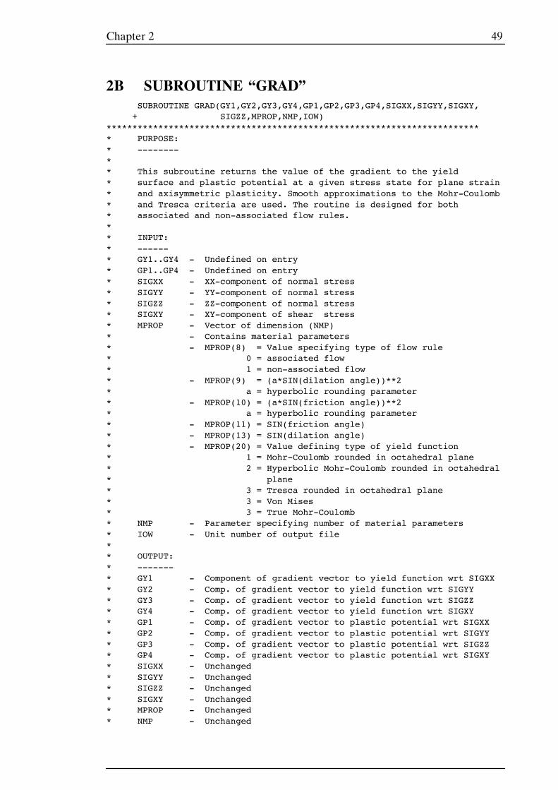
49Chapter 2
2B SUBROUTINE “GRAD”SUBROUTINE GRAD(GY1,GY2,GY3,GY4,GP1,GP2,GP3,GP4,SIGXX,SIGYY,SIGXY,+ SIGZZ,MPROP,NMP,IOW)
************************************************************************* PURPOSE:* --------** This subroutine returns the value of the gradient to the yield* surface and plastic potential at a given stress state for plane strain* and axisymmetric plasticity. Smooth approximations to the Mohr-Coulomb* and Tresca criteria are used. The routine is designed for both* associated and non-associated flow rules.** INPUT:* ------* GY1..GY4 - Undefined on entry* GP1..GP4 - Undefined on entry* SIGXX - XX-component of normal stress* SIGYY - YY-component of normal stress* SIGZZ - ZZ-component of normal stress* SIGXY - XY-component of shear stress* MPROP - Vector of dimension (NMP)* - Contains material parameters* - MPROP(8) = Value specifying type of flow rule* 0 = associated flow* 1 = non-associated flow* - MPROP(9) = (a*SIN(dilation angle))**2* a = hyperbolic rounding parameter* - MPROP(10) = (a*SIN(friction angle))**2* a = hyperbolic rounding parameter* - MPROP(11) = SIN(friction angle)* - MPROP(13) = SIN(dilation angle)* - MPROP(20) = Value defining type of yield function* 1 = Mohr-Coulomb rounded in octahedral plane* 2 = Hyperbolic Mohr-Coulomb rounded in octahedral* plane* 3 = Tresca rounded in octahedral plane* 3 = Von Mises* 3 = True Mohr-Coulomb* NMP - Parameter specifying number of material parameters* IOW - Unit number of output file** OUTPUT:* -------* GY1 - Component of gradient vector to yield function wrt SIGXX* GY2 - Comp. of gradient vector to yield function wrt SIGYY* GY3 - Comp. of gradient vector to yield function wrt SIGZZ* GY4 - Comp. of gradient vector to yield function wrt SIGXY* GP1 - Comp. of gradient vector to plastic potential wrt SIGXX* GP2 - Comp. of gradient vector to plastic potential wrt SIGYY* GP3 - Comp. of gradient vector to plastic potential wrt SIGZZ* GP4 - Comp. of gradient vector to plastic potential wrt SIGXY* SIGXX - Unchanged* SIGYY - Unchanged* SIGZZ - Unchanged* SIGXY - Unchanged* MPROP - Unchanged* NMP - Unchanged
50 Chapter 2
* FLAG - Unchanged* IOW - Unchanged** SUBROUTINES CALLED: NONE* -------------------** PROGRAMMER: Andrew Abbo* -----------** LAST MODIFIED: May 1993 Andrew Abbo* --------------*************************************************************************
INTEGER YFTYPE,NMP,IOWINTEGER FLOW
*DOUBLE PRECISION SIGXX,SIGYY,SIGZZ,SIGXYDOUBLE PRECISION SPHI,SPSI,ASPHI2,ASPSI2DOUBLE PRECISION DSIGX,DSIGY,DSIGZDOUBLE PRECISION THETA,SIGM,J2,J3,SBAR,ALPHADOUBLE PRECISION STA,CTA,C3TA,S3TA,T3TADOUBLE PRECISION A,B,K,DKDOUBLE PRECISION C1,C2,C3DOUBLE PRECISION GY1,GY2,GY3,GY4DOUBLE PRECISION GP1,GP2,GP3,GP4
*DOUBLE PRECISION MPROP(NMP)
** Set constants*
INTEGER RMC,HRMC,TR,ASSOC,VM,MCPARAMETER( RMC=1,HRMC=2,TR=3,VM=4,MC=5 )PARAMETER( ASSOC=0 )
*DOUBLE PRECISION TINYPARAMETER( TINY = 1.0D-10 )
*DOUBLE PRECISION J2TOLPARAMETER( J2TOL = 1.0D-20 )
*DOUBLE PRECISION C004P5,C000P5,CP3333PARAMETER( C004P5 = 4.5D0 )PARAMETER( C000P5 = 0.5D0 )PARAMETER( CP3333 = 0.333333333333333D0 )
*DOUBLE PRECISION C00000,C00001,C00002,C00003,C00004PARAMETER( C00000 = 0.0D0 )PARAMETER( C00001 = 1.0D0 )PARAMETER( C00002 = 2.0D0 )PARAMETER( C00003 = 3.0D0 )PARAMETER( C00004 = 4.0D0 )
*DOUBLE PRECISION C000R3,C00IR3,CP8660PARAMETER( C000R3 = 1.732050807568877D0 )PARAMETER( C00IR3 = 0.5773502691896258D0 )PARAMETER( CP8660 = 0.866025403784439D0 )
*DOUBLE PRECISION CRADPARAMETER (CRAD =0.017453292519943D0)
*
51Chapter 2
* Constants for rounded K function*
DOUBLE PRECISION A1,A2,B1,B2,ATTRAN** Rounding constants for theta > 25 degrees*
PARAMETER( A1 = 1.432052062044227D0 )PARAMETER( A2 = 0.406941858374615D0 )PARAMETER( B1 = 0.544290524902313D0 )PARAMETER( B2 = 0.673903324498392D0 )PARAMETER( ATTRAN=0.436332312998582D0 )
** Rounding constants for theta > 29.5 degrees** PARAMETER( A1 = 7.138654723242523D0 , A2 = 6.112267270920722D0 )* PARAMETER( B1 = 6.270447753139696D0 , B2 = 6.398760841429511D0 )* PARAMETER( ATTRAN = 0.514872129338327D0 )** Calculate value of invariants for the current stress state.*
SIGM = CP3333*(SIGXX+SIGYY+SIGZZ)*
DSIGX = SIGXX-SIGMDSIGY = SIGYY-SIGMDSIGZ = SIGZZ-SIGMJ2 = C000P5*(DSIGX*DSIGX+DSIGY*DSIGY+DSIGZ*DSIGZ) + SIGXY*SIGXYJ3= DSIGZ*(DSIGX*DSIGY-SIGXY*SIGXY)
*SBAR=SQRT(J2)
** Store type of flow rule* If MPROP(8)=1 then have non-associated flow rule* If have associated flow rule, then the gradients to the plastic* potential and the yield function will be set equal*
FLOW=INT(MPROP(8))** Extract form of yield function from MPROP vector*
YFTYPE=INT(MPROP(20))*
IF (YFTYPE.EQ.RMC) THEN*-----------------------------------------------------------------------
* Rounded Mohr-Coulomb yield function*
IF (J2.GT.J2TOL) THEN** Calculate third stress invariant*
S3TA = -C004P5*J3/(C000R3*SBAR*J2)IF (S3TA.LT.-C00001) THENWRITE(IOW,’(’’ *** S3TA set equal -1 ***’’,F12.5)’)S3TAWRITE(IOW,’(’’ J2,J3,SIGM ’’,4E14.5)’) J2,J3,SIGMWRITE(IOW,’(’’ J2,J3 ’’,4E14.5)’) DSIGX,DSIGY,DSIGZ,SIGXYS3TA = -C00001
ELSEIF (S3TA.GT.C00001) THENWRITE(IOW,’(’’ *** S3TA set equal +1 ***’’,F12.5)’)S3TAWRITE(IOW,’(’’ J2,J3,SIGM ’’,4E14.5)’) J2,J3,SIGMWRITE(IOW,’(’’ J2,J3 ’’,4E14.5)’) DSIGX,DSIGY,DSIGZ,SIGXY
52 Chapter 2
S3TA = C00001ENDIFTHETA = CP3333*ASIN(S3TA)
*ELSE
** Special case of zero deviatoric stress*
WRITE(IOW,’(’’ *** WARNING IN SUBROUTINE GRAD ***’’)’)WRITE(IOW,’(’’ ZERO DEVIATORIC STRESS STATE ’’)’)
*J2 = TINY*TINYSBAR = TINYTHETA = C00000S3TA = C00000
*ENDIF
** Set value of material parameters used in gradient calculations*
SPHI = MPROP(11)** Calculate gradient constants*
IF (ABS(THETA).LT.ATTRAN) THEN** Unrounded surface*
CTA = COS(THETA)C3TA = CTA*(C00004*CTA*CTA-C00003)T3TA = S3TA/C3TASTA = S3TA/(C00004*CTA*CTA-C00001)K = CTA-STA*SPHI*C00IR3DK = STA+CTA*SPHI*C00IR3
*C1 = SPHIC2 = K+T3TA*DKC3 = CP8660*DK/C3TA
*ELSE
** Rounded surface*
IF (THETA.GT.C00000) THENA = A1 + A2*SPHIB = B1 + B2*SPHI
ELSEA = A1 - A2*SPHIB = - B1 + B2*SPHI
ENDIF*
C1 = SPHIC2 = A + C00002*B*S3TAC3 = CP8660*C00003*B
*ENDIF
*ELSEIF (YFTYPE.EQ.HRMC) THEN
*-----------------------------------------------------------------------
53Chapter 2
* Hyperbolic Rounded Mohr-Coulomb yield function*
IF (J2.GT.J2TOL) THEN** Calculate third stress invariant*
S3TA = -C004P5*J3/(C000R3*SBAR*J2)IF (S3TA.LT.-C00001) THENWRITE(IOW,’(’’ *** S3TA set equal -1 ***’’,F12.5)’)S3TAWRITE(IOW,’(’’ J2,J3,SIGM ’’,4E14.5)’) J2,J3,SIGMWRITE(IOW,’(’’ J2,J3 ’’,4E14.5)’) DSIGX,DSIGY,DSIGZ,SIGXYS3TA = -C00001
ELSEIF (S3TA.GT.C00001) THENWRITE(IOW,’(’’ *** S3TA set equal +1 ***’’,F12.5)’)S3TAWRITE(IOW,’(’’ J2,J3,SIGM ’’,4E14.5)’) J2,J3,SIGMWRITE(IOW,’(’’ J2,J3 ’’,4E14.5)’) DSIGX,DSIGY,DSIGZ,SIGXYS3TA = C00001
ENDIFTHETA = CP3333*ASIN(S3TA)
*ELSE
** Special case of zero deviatoric stress*
WRITE(IOW,’(’’ *** WARNING IN SUBROUTINE GRAD ***’’)’)WRITE(IOW,’(’’ ZERO DEVIATORIC STRESS STATE ’’)’)
*J2 = TINY*TINYSBAR = TINYTHETA = C00000S3TA = C00000
*ENDIF
** Set value of material parameters used in gradient calculations*
SPHI = MPROP(11)ASPHI2 = MPROP(10)
** Calculate gradient constants*
IF (ABS(THETA).LT.ATTRAN) THEN** Unrounded surface*
CTA = COS(THETA)C3TA = CTA*(C00004*CTA*CTA-C00003)T3TA = S3TA/C3TASTA = S3TA/(C00004*CTA*CTA-C00001)K = CTA-STA*SPHI*C00IR3DK = STA+CTA*SPHI*C00IR3
*C1 = SPHIC2 = K+T3TA*DKC3 = CP8660*DK/C3TA
*ELSE
** Rounded surface*
54 Chapter 2
IF (THETA.GT.C00000) THENA = A1 + A2*SPHIB = B1 + B2*SPHI
ELSEA = A1 - A2*SPHIB = - B1 + B2*SPHI
ENDIF*
K = A-B*S3TA*
C1 = SPHIC2 = A + C00002*B*S3TAC3 = CP8660*C00003*B
*ENDIF
** Adjust coefficients for hyperbolic Mohr-Coulomb surface*
IF (ASPHI2.GT.C00000) THENALPHA = SBAR*KALPHA = K/SQRT(ALPHA*ALPHA + ASPHI2)C2 = C2*ALPHAC3 = C3*ALPHA
ENDIF*
ELSEIF ( YFTYPE.EQ.TR) THEN*-----------------------------------------------------------------------
* Tresca Yield Function*
IF (J2.GT.C00000) THEN** Calculate third stress invariant*
S3TA = -C004P5*J3/(C000R3*SBAR*J2)IF (S3TA.LT.-C00001) THENS3TA = -C00001
ELSEIF (S3TA.GT.C00001) THENS3TA = C00001
ENDIFTHETA = CP3333*ASIN(S3TA)
*ELSE
** Cannot have yielding at zero deviatoric stress for Tresca*
WRITE(IOW,’(’’ *** ERROR IN SUBROUTINE GRAD ***’’)’)WRITE(IOW,’(’’ ZERO J2 INVAR. FOR TRESCA YIELD FUNCTION’’)’)STOP
*ENDIF
** Calculate gradient constants*
IF (ABS(THETA).LT.ATTRAN) THEN** Unrounded surface*
CTA = COS(THETA)C3TA = CTA*(C00004*CTA*CTA-C00003)
55Chapter 2
T3TA = S3TA/C3TASTA = S3TA/(C00004*CTA*CTA-C00001)
*K = CTADK = STA
*C1 = C00000C2 = CTA+T3TA*STAC3 = CP8660*STA/C3TA
*ELSE
** Rounded surface*
A = A1IF (THETA.GT.C00000) THENB = B1
ELSEB = - B1
ENDIF*
C1 = C00000C2 = A + C00002*B*S3TAC3 = CP8660*C00003*B
*ENDIFFLOW=ASSOC
*ELSEIF ( YFTYPE.EQ.VM) THEN
*-----------------------------------------------------------------------* Von Mises Yield Function** Calculate gradient coefficients*
C1 = C00000C2 = C000R3C3 = C00000FLOW=ASSOC
*ELSEIF ( YFTYPE.EQ.MC) THEN
*-----------------------------------------------------------------------* Mohr-Coulomb yield function*
IF (J2.GT.C00000) THEN** Calculate third stress invariant*
S3TA = -C004P5*J3/(C000R3*SBAR*J2)IF (S3TA.LT.-C00001) THENS3TA = -C00001
ELSEIF (S3TA.GT.C00001) THENS3TA = C00001
ENDIFTHETA = CP3333*ASIN(S3TA)
*ELSE
** Special case of zero deviatoric stress*
WRITE(IOW,’(’’ *** WARNING IN SUBROUTINE GRAD ***’’)’)
56 Chapter 2
WRITE(IOW,’(’’ ZERO DEVIATORIC STRESS STATE ’’)’)J2 = TINYSBAR = TINY*TINYTHETA = C00000S3TA = C00000
*ENDIF
** Set value of material parameters used in gradient calculations*
SPHI = MPROP(11)*
CTA = COS(THETA)C3TA = CTA*(C00004*CTA*CTA-C00003)T3TA = S3TA/C3TA
** Calculate K function and its derivative wrt theta DK*
STA = S3TA/(C00004*CTA*CTA-C00001)K = CTA-STA*SPHI*C00IR3DK = STA+CTA*SPHI*C00IR3
** Calculate gradient coefficients for Mohr-Coulomb surface*
C1 = SPHIC2 = K+T3TA*DKC3 = (CP8660*DK)/C3TA
*ELSE
** Invalid yield function type*
WRITE(IOW,’(’’ *** ERROR IN SUBROUTINE GRAD ***’’)’)WRITE(IOW,’(’’ INVALID YIELD FUNCTION - YFTYPE = ’’,I4)’)YFTYPESTOP
*ENDIF
** Compose gradient to yield function*
C2 = C2*C000P5C1 = C1*CP3333IF ((YFTYPE.EQ.HRMC).AND.(ASPHI2.GT.C00000)) THENGY1=C1+C2*(DSIGX)+C3*((DSIGY*DSIGZ)/SBAR + CP3333*SBAR)GY2=C1+C2*(DSIGY)+C3*((DSIGX*DSIGZ)/SBAR + CP3333*SBAR)GY3=C00002*(C2*(SIGXY) - C3*(SIGXY*DSIGZ/SBAR))GY4=C1+C2*(DSIGZ)+C3*((DSIGX*DSIGY-SIGXY*SIGXY)/SBAR+CP3333*SBAR)
ELSEGY1=C1+C2*(DSIGX/SBAR)+C3*((DSIGY*DSIGZ)/J2 + CP3333)GY2=C1+C2*(DSIGY/SBAR)+C3*((DSIGX*DSIGZ)/J2 + CP3333)GY3=C00002*(C2*(SIGXY/SBAR) - C3*(SIGXY*DSIGZ/J2))GY4=C1+C2*(DSIGZ/SBAR)+C3*((DSIGX*DSIGY-SIGXY*SIGXY)/J2+CP3333)
ENDIF** Calculate gradient to potential for associated case*
IF (FLOW.EQ.ASSOC) THENGP1 = GY1GP2 = GY2GP3 = GY3
57Chapter 2
GP4 = GY4RETURN
ENDIF** If non-associated flow calculate gradient to plastic potential* Assume that the plastic potential has the same form as the yield* function except that the dilation angle is substituted for the* friction angle*
IF (YFTYPE.EQ.RMC) THEN*-----------------------------------------------------------------------
* Rounded Mohr-Coulomb plastic potential* Extract material parameters*
SPSI = MPROP(13)** Calculate K function and its derivative wrt theta*
IF (ABS(THETA).LT.ATTRAN) THEN** Unrounded surface*
K = CTA-STA*SPSI*C00IR3DK = STA+CTA*SPSI*C00IR3
*C1 = SPSIC2 = K+T3TA*DKC3 = CP8660*DK/C3TA
*ELSE
** Rounded surface*
IF (THETA.GT.C00000) THENA = A1 + A2*SPSIB = B1 + B2*SPSI
ELSEA = A1 - A2*SPSIB = - B1 + B2*SPSI
ENDIF*
C1 = SPSIC2 = A + C00002*B*S3TAC3 = CP8660*C00003*B
*ENDIF
*ELSEIF (YFTYPE.EQ.HRMC) THEN
*-----------------------------------------------------------------------
* Hyperbolic Rounded Mohr-Coulomb plastic potential* Extract material parameters*
SPSI = MPROP(13)ASPSI2 = MPROP(9)
** Calculate K function and its derivative wrt theta*
IF (ABS(THETA).LT.ATTRAN) THEN
58 Chapter 2
** Unrounded surface*
K = CTA-STA*SPSI*C00IR3DK = STA+CTA*SPSI*C00IR3
*C1 = SPSIC2 = K+T3TA*DKC3 = CP8660*DK/C3TA
*ELSE
** Rounded surface*
IF (THETA.GT.C00000) THENA = A1 + A2*SPSIB = B1 + B2*SPSI
ELSEA = A1 - A2*SPSIB = - B1 + B2*SPSI
ENDIFK = A-B*S3TA
*C1 = SPSIC2 = A + C00002*B*S3TAC3 = CP8660*C00003*B
*ENDIF
** Adjust coefficients for hyperbolic Mohr-Coulomb surface*
IF (ASPSI2.GT.C00000) THENALPHA = SBAR*KALPHA = K/SQRT(ALPHA*ALPHA + ASPSI2)C2 = C2*ALPHAC3 = C3*ALPHA
ENDIF*
ELSEIF ( YFTYPE.EQ.VM) THEN*-----------------------------------------------------------------------* Von Mises Plastic Potential** Calculate gradient coefficients*
C1 = C00000C2 = C000R3C3 = C00000
*ELSEIF (YFTYPE.EQ.MC) THEN
** Mohr-Coulomb plastic potential** Set value of material parameters used in gradient calculations*
SPSI = MPROP(13)*
CTA = COS(THETA)C3TA = CTA*(C00004*CTA*CTA-C00003)T3TA = S3TA/C3TA
*
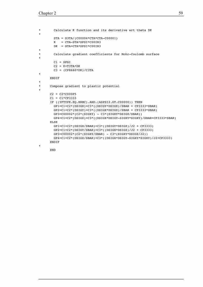
59Chapter 2
* Calculate K function and its derivative wrt theta DK*
STA = S3TA/(C00004*CTA*CTA-C00001)K = CTA-STA*SPSI*C00IR3DK = STA+CTA*SPSI*C00IR3
** Calculate gradient coefficients for Mohr-Coulomb surface*
C1 = SPSIC2 = K+T3TA*DKC3 = (CP8660*DK)/C3TA
*ENDIF
** Compose gradient to plastic potential*
C2 = C2*C000P5C1 = C1*CP3333IF ((YFTYPE.EQ.HRMC).AND.(ASPSI2.GT.C00000)) THENGP1=C1+C2*(DSIGX)+C3*((DSIGY*DSIGZ)/SBAR + CP3333*SBAR)GP2=C1+C2*(DSIGY)+C3*((DSIGX*DSIGZ)/SBAR + CP3333*SBAR)GP3=C00002*(C2*(SIGXY) - C3*(SIGXY*DSIGZ/SBAR))GP4=C1+C2*(DSIGZ)+C3*((DSIGX*DSIGY-SIGXY*SIGXY)/SBAR+CP3333*SBAR)
ELSEGP1=C1+C2*(DSIGX/SBAR)+C3*((DSIGY*DSIGZ)/J2 + CP3333)GP2=C1+C2*(DSIGY/SBAR)+C3*((DSIGX*DSIGZ)/J2 + CP3333)GP3=C00002*(C2*(SIGXY/SBAR) - C3*(SIGXY*DSIGZ/J2))GP4=C1+C2*(DSIGZ/SBAR)+C3*((DSIGX*DSIGY-SIGXY*SIGXY)/J2+CP3333)
ENDIF*
END
61Chapter 3
CHAPTER 3
INTEGRATION OF STRESS-STRAIN
RELATIONS
62Chapter 3
3.1 INTRODUCTION
The first part of this Chapter discusses the practical implementation of an explicit
modified Euler scheme for integrating elastoplastic constitutive laws in finite
element analysis. This algorithm is based on the method of Sloan (1987) and
controls the error in the computed stresses by using a local error measure to
automatically subincrement and integrate the applied strain increment. It
incorporates a number of important new refinements which enhance the efficiency
and robustness of explicit subincrementation techniques. The next part of the
Chapter describes two implicit backward Euler schemes as described by Crisfield
(1991). These methods have been used widely in metal plasticity studies but have
had limited application to geotechnical constitutive models.
The last part of the Chapter compares the performance of the explicit modified
Euler scheme against the performance of the implicit backward Euler schemes.
To test the efficiency and robustness of these algorithms, the non-trivial boundary
value problem of a rigid strip footing resting on a Tresca or Mohr-Coulomb layer
is used. For the Mohr-Coulomb soil, results are presented for both associated and
nonassociated flow rules. The explicit modified Euler scheme with substepping
is shown to be very competitive with an implicit backward Euler return scheme,
and has the added advantage that the error in the computed stresses (for a given
mesh and load path) may be controlled to a desired level. A further attraction
of the explicit method is that it requires only first derivatives (with respect to the
stresses) of the yield surface and plastic potential. The second derivatives needed
for the implicit methods are both difficult and expensive to compute for many
geotechnical models. The results for the footing problems suggest that the implicit
schemes do not perform well in the vicinity of the corners of the Tresca and
Mohr-Coulomb yield criteria, even when they are rounded, and special strategies
may be required.
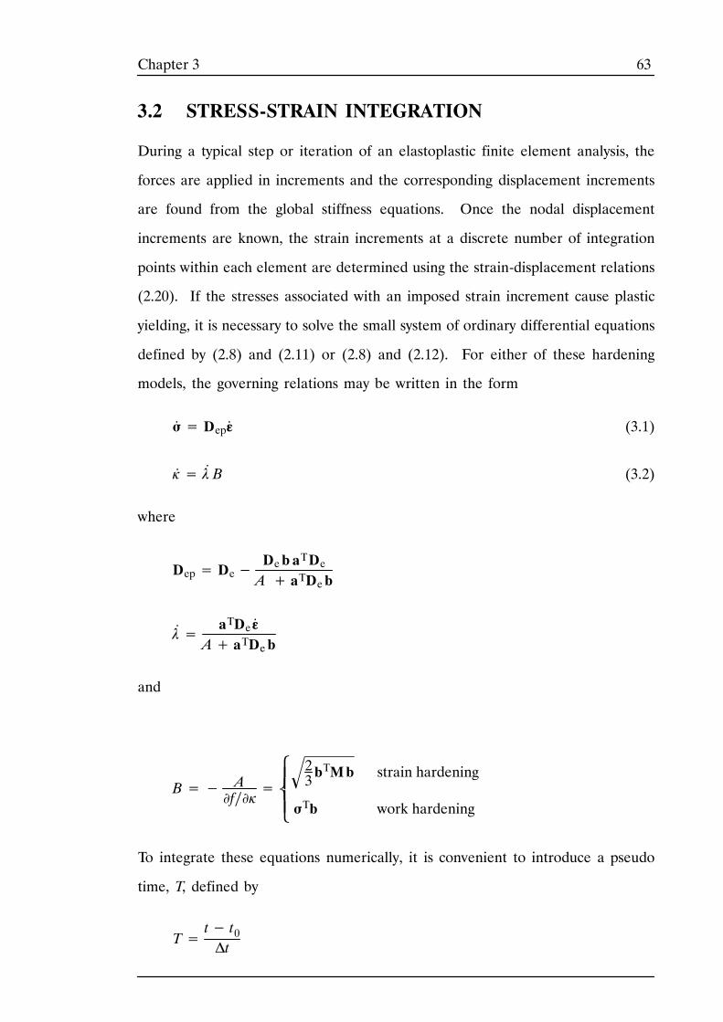
63Chapter 3
3.2 STRESS-STRAIN INTEGRATION
During a typical step or iteration of an elastoplastic finite element analysis, the
forces are applied in increments and the corresponding displacement increments
are found from the global stiffness equations. Once the nodal displacement
increments are known, the strain increments at a discrete number of integration
points within each element are determined using the strain-displacement relations
(2.20). If the stresses associated with an imposed strain increment cause plastic
yielding, it is necessary to solve the small system of ordinary differential equations
defined by (2.8) and (2.11) or (2.8) and (2.12). For either of these hardening
models, the governing relations may be written in the form
σ. = Depε
. (3.1)
À. = λ
.B (3.2)
where
Dep= De−Deb aTDeA + aTDeb
λ.=
aTDeε.
A+ aTDeb
and
B=− A∂f∕∂À
=⎪⎪⎨⎧
⎩
23bTMb
σTb
strain hardening
work hardening
To integrate these equations numerically, it is convenient to introduce a pseudo
time, T, defined by
T=t− t0Δt
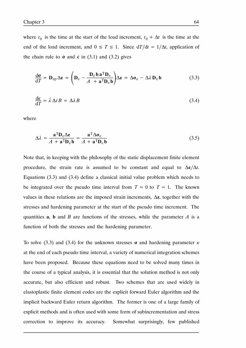
64Chapter 3
where t0 is the time at the start of the load increment, t0+ Δt is the time at the
end of the load increment, and 0≤ T≤ 1. Since dT∕dt= 1∕Δt, application of
the chain rule to σ. and À. in (3.1) and (3.2) gives
dσdT= DepΔε= De− Deb aTDe
A + aTDebΔε= Δσe− ΔλDe b (3.3)
dÀdT= λ
.Δt B= ΔλB (3.4)
where
Δλ=aTDeΔεA+ aTDeb
=aTΔσe
A+ aTDeb(3.5)
Note that, in keeping with the philosophy of the static displacement finite element
procedure, the strain rate is assumed to be constant and equal to Δε∕Δt.
Equations (3.3) and (3.4) define a classical initial value problem which needs to
be integrated over the pseudo time interval from T= 0 to T= 1. The known
values in these relations are the imposed strain increments, Δε, together with the
stresses and hardening parameter at the start of the pseudo time increment. The
quantities a, b and B are functions of the stresses, while the parameter A is a
function of both the stresses and the hardening parameter.
To solve (3.3) and (3.4) for the unknown stresses σ and hardening parameter À
at the end of each pseudo time interval, a variety of numerical integration schemes
have been proposed. Because these equations need to be solved many times in
the course of a typical analysis, it is essential that the solution method is not only
accurate, but also efficient and robust. Two schemes that are used widely in
elastoplastic finite element codes are the explicit forward Euler algorithm and the
implicit backward Euler return algorithm. The former is one of a large family of
explicit methods and is often used with some form of subincrementation and stress
correction to improve its accuracy. Somewhat surprisingly, few published
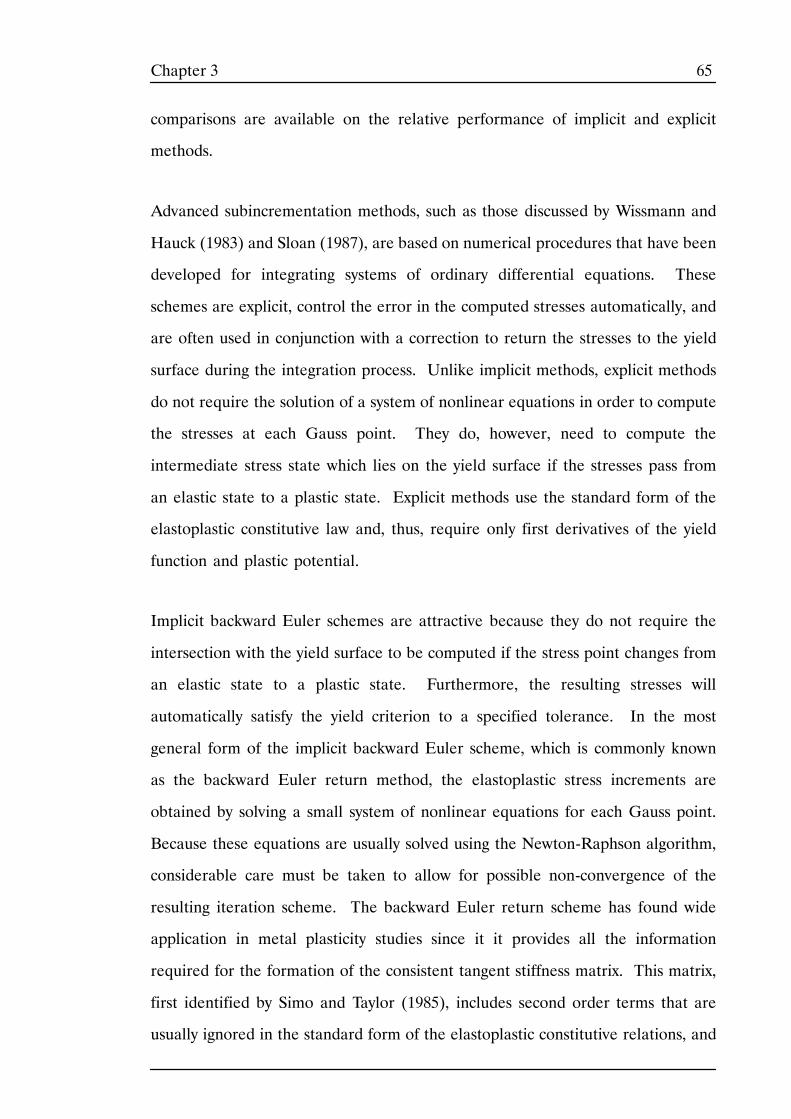
65Chapter 3
comparisons are available on the relative performance of implicit and explicit
methods.
Advanced subincrementation methods, such as those discussed by Wissmann and
Hauck (1983) and Sloan (1987), are based on numerical procedures that have been
developed for integrating systems of ordinary differential equations. These
schemes are explicit, control the error in the computed stresses automatically, and
are often used in conjunction with a correction to return the stresses to the yield
surface during the integration process. Unlike implicit methods, explicit methods
do not require the solution of a system of nonlinear equations in order to compute
the stresses at each Gauss point. They do, however, need to compute the
intermediate stress state which lies on the yield surface if the stresses pass from
an elastic state to a plastic state. Explicit methods use the standard form of the
elastoplastic constitutive law and, thus, require only first derivatives of the yield
function and plastic potential.
Implicit backward Euler schemes are attractive because they do not require the
intersection with the yield surface to be computed if the stress point changes from
an elastic state to a plastic state. Furthermore, the resulting stresses will
automatically satisfy the yield criterion to a specified tolerance. In the most
general form of the implicit backward Euler scheme, which is commonly known
as the backward Euler return method, the elastoplastic stress increments are
obtained by solving a small system of nonlinear equations for each Gauss point.
Because these equations are usually solved using the Newton-Raphson algorithm,
considerable care must be taken to allow for possible non-convergence of the
resulting iteration scheme. The backward Euler return scheme has found wide
application in metal plasticity studies since it it provides all the information
required for the formation of the consistent tangent stiffness matrix. This matrix,
first identified by Simo and Taylor (1985), includes second order terms that are
usually ignored in the standard form of the elastoplastic constitutive relations, and
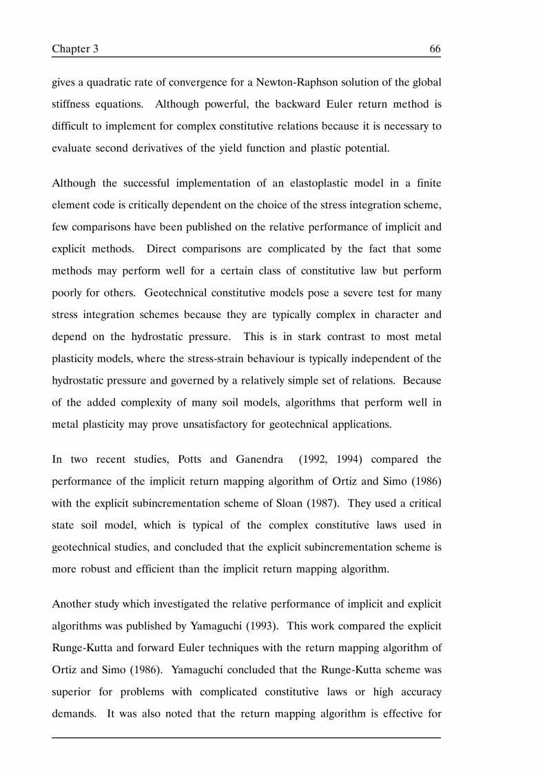
66Chapter 3
gives a quadratic rate of convergence for a Newton-Raphson solution of the global
stiffness equations. Although powerful, the backward Euler return method is
difficult to implement for complex constitutive relations because it is necessary to
evaluate second derivatives of the yield function and plastic potential.
Although the successful implementation of an elastoplastic model in a finite
element code is critically dependent on the choice of the stress integration scheme,
few comparisons have been published on the relative performance of implicit and
explicit methods. Direct comparisons are complicated by the fact that some
methods may perform well for a certain class of constitutive law but perform
poorly for others. Geotechnical constitutive models pose a severe test for many
stress integration schemes because they are typically complex in character and
depend on the hydrostatic pressure. This is in stark contrast to most metal
plasticity models, where the stress-strain behaviour is typically independent of the
hydrostatic pressure and governed by a relatively simple set of relations. Because
of the added complexity of many soil models, algorithms that perform well in
metal plasticity may prove unsatisfactory for geotechnical applications.
In two recent studies, Potts and Ganendra (1992, 1994) compared the
performance of the implicit return mapping algorithm of Ortiz and Simo (1986)
with the explicit subincrementation scheme of Sloan (1987). They used a critical
state soil model, which is typical of the complex constitutive laws used in
geotechnical studies, and concluded that the explicit subincrementation scheme is
more robust and efficient than the implicit return mapping algorithm.
Another study which investigated the relative performance of implicit and explicit
algorithms was published by Yamaguchi (1993). This work compared the explicit
Runge-Kutta and forward Euler techniques with the return mapping algorithm of
Ortiz and Simo (1986). Yamaguchi concluded that the Runge-Kutta scheme was
superior for problems with complicated constitutive laws or high accuracy
demands. It was also noted that the return mapping algorithm is effective for
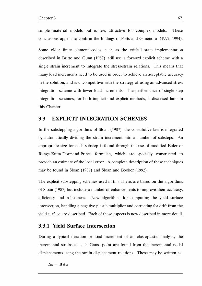
67Chapter 3
simple material models but is less attractive for complex models. These
conclusions appear to confirm the findings of Potts and Ganendra (1992, 1994).
Some older finite element codes, such as the critical state implementation
described in Britto and Gunn (1987), still use a forward explicit scheme with a
single strain increment to integrate the stress-strain relations. This means that
many load increments need to be used in order to achieve an acceptable accuracy
in the solution, and is uncompetitive with the strategy of using an advanced stress
integration scheme with fewer load increments. The performance of single step
integration schemes, for both implicit and explicit methods, is discussed later in
this Chapter.
3.3 EXPLICIT INTEGRATION SCHEMES
In the substepping algorithms of Sloan (1987), the constitutive law is integrated
by automatically dividing the strain increment into a number of substeps. An
appropriate size for each substep is found through the use of modified Euler or
Runge-Kutta-Dormand-Prince formulae, which are specially constructed to
provide an estimate of the local error. A complete description of these techniques
may be found in Sloan (1987) and Sloan and Booker (1992).
The explicit substepping schemes used in this Thesis are based on the algorithms
of Sloan (1987) but include a number of enhancements to improve their accuracy,
efficiency and robustness. New algorithms for computing the yield surface
intersection, handling a negative plastic multiplier and correcting for drift from the
yield surface are described. Each of these aspects is now described in more detail.
3.3.1 Yield Surface Intersection
During a typical iteration or load increment of an elastoplastic analysis, the
incremental strains at each Gauss point are found from the incremental nodal
displacements using the strain-displacement relations. These may be written as
Δε= BΔu
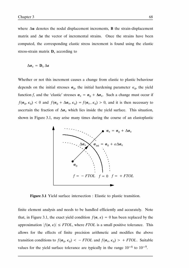
68Chapter 3
where Δu denotes the nodal displacement increments, B the strain-displacement
matrix and Δε the vector of incremental strains. Once the strains have been
computed, the corresponding elastic stress increment is found using the elastic
stress-strain matrix De according to
Δσe= De Δε
Whether or not this increment causes a change from elastic to plastic behaviour
depends on the initial stresses σ0, the initial hardening parameter À0, the yield
function f, and the ‘elastic’ stresses σe= σ0+ Δσe. Such a change must occur if
f (σ0, À0)< 0 and f (σ0+ Δσe, À0)= f (σe , À0)> 0, and it is then necessary to
ascertain the fraction of Δσe which lies inside the yield surface. This situation,
shown in Figure 3.1, may arise many times during the course of an elastoplastic
Δσe
σe= σ0+ Δσe
σ0
f= 0
Figure 3.1 Yield surface intersection : Elastic to plastic transition.
f=+ FTOLf=− FTOL
σint= σ0+ αΔσe
finite element analysis and needs to be handled efficiently and accurately. Note
that, in Figure 3.1, the exact yield condition f (σ, À)= 0 has been replaced by the
approximation f (σ, À) ≤ FTOL, where FTOL is a small positive tolerance. This
allows for the effects of finite precision arithmetic and modifies the above
transition conditions to f (σ0, À0)<− FTOL and f (σe, À0)>+ FTOL. Suitable
values for the yield surface tolerance are typically in the range 10---6 to 10---9.

69Chapter 3
The problem of locating the stresses at the yield surface intersection point, σint,
and hence the elastic portion of Δσe, is equivalent to finding the scalar quantity
α which satisfies the nonlinear equation
f (σ0+ αΔσe, À0)= f (σint, À0)= 0 (3.6)
An α value of zero indicates that Δσe causes purely plastic deformation, while an
α value of unity indicates that Δσe causes purely elastic deformation. Thus, for
an elastic to plastic transition, α lies within the range 0< α< 1, and the elastic
part of the stress increment is given by αΔσe.
Since equation (3.6) defines a single nonlinear equation in the variable α, it can
be solved using the well known methods of bisection, regula-falsi, modified
regula-falsi, secant, and Newton-Raphson (see, for example, Conte and de Boor
(1980) for a detailed discussion of these algorithms). The first three schemes have
the advantage that they always bound the solution for α within a known interval
and, thus, are unconditionally convergent for continuous yield functions. The
Newton-Raphson and secant techniques, discussed by Sloan (1987), offer rapid
convergence rates but may diverge in some circumstances because they do not
constrain the solution. The modified regula-falsi procedure is ideally suited to
solving the yield surface intersection problem defined by (3.6) since it is
unconditionally convergent, does not require the use of derivatives, and typically
converges in four or five iterations (even when used with stringent values for the
tolerance FTOL). The complete modified regula-falsi algorithm is detailed below.
Modified Regula-falsi Intersection Scheme
1. Enter with stresses σ0 and hardening parameter À0, the stress increment
Δσe, initial values of α0 and α1 bounding the intersection with the yield
surface, and the maximum number of iterations MAXITS.
2. Set Fsave= f (σ0 , À0), F0= f (σ0+ α0Δσe ,À0) and F1= f (σ0+ α1Δσe,À0)
3. Do steps 4 to 7 MAXITS times
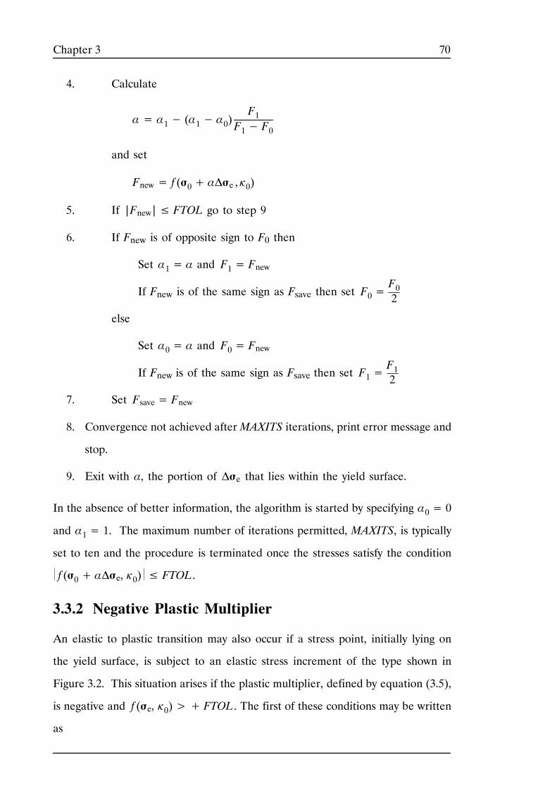
70Chapter 3
4. Calculate
α= α1− (α1− α0)F1
F1− F0
and set
Fnew= f (σ0+ αΔσe , À0)
5. If |Fnew|≤ FTOL go to step 9
6. If Fnew is of opposite sign to F0 then
Set α1= α and F1= Fnew
If Fnew is of the same sign as Fsave then set F0=F02
else
Set α0= α and F0= Fnew
If Fnew is of the same sign as Fsave then set F1=F12
7. Set Fsave= Fnew
8. Convergence not achieved afterMAXITS iterations, print error message and
stop.
9. Exit with α, the portion of Δσe that lies within the yield surface.
In the absence of better information, the algorithm is started by specifying α0= 0
and α1= 1. The maximum number of iterations permitted, MAXITS, is typically
set to ten and the procedure is terminated once the stresses satisfy the condition
f (σ0+ αΔσe, À0) ≤ FTOL.
3.3.2 Negative Plastic Multiplier
An elastic to plastic transition may also occur if a stress point, initially lying on
the yield surface, is subject to an elastic stress increment of the type shown in
Figure 3.2. This situation arises if the plastic multiplier, defined by equation (3.5),
is negative and f (σe, À0)>+ FTOL. The first of these conditions may be written
as
71Chapter 3
Δσe
f=+ FTOL
σe= σ0+ Δσe
σ0f= 0
f=−FTOL
Figure 3.2 Yield surface intersection: Negative plastic multiplier.
σint= σ0+ αΔσe
a0=∂f∂σ
θ
Δλ=aT0 Δσe
A0+ aT0Deb0< 0
where the quantities A0, a0, b0 are all evaluated at the initial stress state σ0.
Stress points with negative plastic multipliers can occur under monotonic loading
of the overall structure, particularly if the trial stress increment Δσe is large as a
result of the use of discrete load increments, and are often found near the tip of
the Mohr-Coulomb yield surface. Because the portion of the stress path that lies
within the yield surface is elastic, the elastoplastic constitutive law need only be
integrated beyond the last intersection point.
In practice, negative plastic multipliers can be detected by computing the cosine
of the angle between a0 and Δσe and checking whether
72Chapter 3
cos θ=aT0 Δσe a0 2 Δσe2
< LTOL
where LTOL is a suitable tolerance. This test is efficient since it avoids the need
to compute Δλ explicitly.
The procedure for finding the yield surface intersection for a negative plastic
multiplier is identical to that discussed in the previous Section, except that a
different set of starting values for α must be used. The situation is complicated
by the fact that the stress increment may in fact cross the yield surface twice, as
shown in Figure 3.2. This possibility is caused by the use of the tolerance FTOL,
which permits the stresses to lie just outside the yield surface, and must be
accounted for. To ensure the modified regula-falsi algorithm isolates the correct
crossing, it is sufficient to determine starting values, α0 and α1, which satisfy
f (σ0+ α0Δσe, À)<− FTOL and f (σ0+ α1Δσe, À)> FTOL. These conditions
guarantee that α0 and α1 bracket the second yield surface intersection. As in the
previous case, α= 0 indicates that Δσe causes purely plastic deformation while
α= 1 indicates that Δσe causes purely elastic deformation. Because it is assumed
that f (σe, À)>+ FTOL, α again must lie within the range 0< α< 1.
One strategy for locating the starting values which bracket the desired crossing is
based on breaking up the trial stress increment Δσe into a number of smaller
subincrements. Each of these is then scanned to see if the yield surface is crossed.
The number of subincrements used in the search, NSUB, is typically set to ten,
although numerical experiments suggest that as few as two subincrements may be
used with only a marginal increase in computation time. In the first iteration, the
subincrement size is set to Δσe∕NSUB, which corresponds to subincrements in α
of Δα= 1∕NSUB. A check is then made to see if the desired crossing lies in any
of the intervals defined by the pairs (αn−1 ,αn ), where αn= αn−1+ nΔα, α0= 0,
and n= 1, 2,. . ., NSUB. Such a crossing occurs if f (σ0+ αn−1Δσe, À)<− FTOL
and f (σ0+ αnΔσe , À)>+ FTOL. A geometric illustration of a successful search
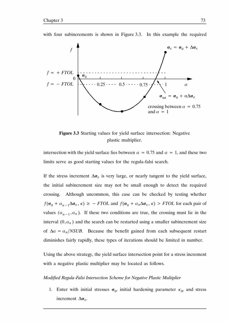
73Chapter 3
with four subincrements is shown in Figure 3.3. In this example the required
σe= σ0+ Δσe
σ0
Figure 3.3 Starting values for yield surface intersection: Negativeplastic multiplier.
σint= σ0+ αΔσe
f=+ FTOL
f=− FTOL
f
α0
0.25 0.5 0.75 1
crossing between α= 0.75and α= 1
intersection with the yield surface lies between α= 0.75 and α= 1, and these two
limits serve as good starting values for the regula-falsi search.
If the stress increment Δσe is very large, or nearly tangent to the yield surface,
the initial subincrement size may not be small enough to detect the required
crossing. Although uncommon, this case can be checked by testing whether
f (σ0+ αn−1Δσe , À)≥− FTOL and f (σ0+ αnΔσe , À)> FTOL for each pair of
values (αn−1 ,αn ). If these two conditions are true, the crossing must lie in the
interval (0,αn ) and the search can be restarted using a smaller subincrement size
of Δα= αn∕NSUB. Because the benefit gained from each subsequent restart
diminishes fairly rapidly, these types of iterations should be limited in number.
Using the above strategy, the yield surface intersection point for a stress increment
with a negative plastic multiplier may be located as follows.
Modified Regula-Falsi Intersection Scheme for Negative Plastic Multiplier
1. Enter with initial stresses σ0, initial hardening parameter À0, and stress
increment Δσe.
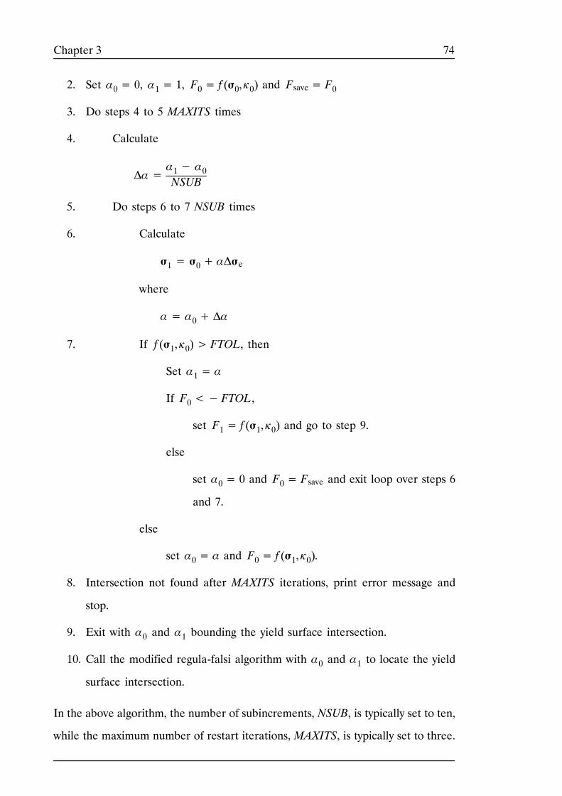
74Chapter 3
2. Set α0= 0, α1= 1, F0= f (σ0,À0) and Fsave= F0
3. Do steps 4 to 5 MAXITS times
4. Calculate
Δα=α1− α0NSUB
5. Do steps 6 to 7 NSUB times
6. Calculate
σ1= σ0+ αΔσe
where
α= α0+ Δα
7. If f (σ1,À0)> FTOL, then
Set α1= α
If F0<−FTOL,
set F1= f (σ1,À0) and go to step 9.
else
set α0= 0 and F0= Fsave and exit loop over steps 6
and 7.
else
set α0= α and F0= f (σ1,À0).
8. Intersection not found after MAXITS iterations, print error message and
stop.
9. Exit with α0 and α1 bounding the yield surface intersection.
10. Call the modified regula-falsi algorithm with α0 and α1 to locate the yield
surface intersection.
In the above algorithm, the number of subincrements, NSUB, is typically set to ten,
while the maximum number of restart iterations, MAXITS, is typically set to three.
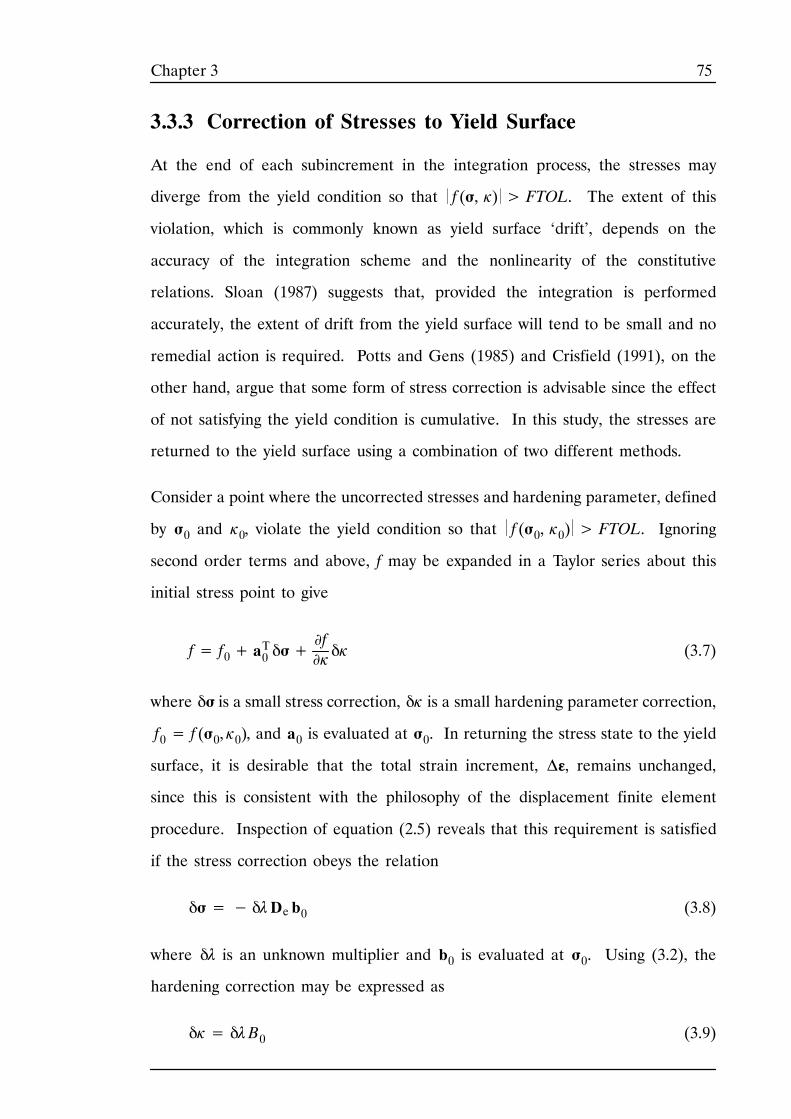
75Chapter 3
3.3.3 Correction of Stresses to Yield Surface
At the end of each subincrement in the integration process, the stresses may
diverge from the yield condition so that f (σ, À) > FTOL. The extent of this
violation, which is commonly known as yield surface ‘drift’, depends on the
accuracy of the integration scheme and the nonlinearity of the constitutive
relations. Sloan (1987) suggests that, provided the integration is performed
accurately, the extent of drift from the yield surface will tend to be small and no
remedial action is required. Potts and Gens (1985) and Crisfield (1991), on the
other hand, argue that some form of stress correction is advisable since the effect
of not satisfying the yield condition is cumulative. In this study, the stresses are
returned to the yield surface using a combination of two different methods.
Consider a point where the uncorrected stresses and hardening parameter, defined
by σ0 and À0, violate the yield condition so that f (σ0, À0) > FTOL. Ignoring
second order terms and above, f may be expanded in a Taylor series about this
initial stress point to give
f= f0+ aT0 δσ+
∂f∂À δÀ (3.7)
where δσ is a small stress correction, δÀ is a small hardening parameter correction,
f0= f (σ0, À0), and a0 is evaluated at σ0. In returning the stress state to the yield
surface, it is desirable that the total strain increment, Δε, remains unchanged,
since this is consistent with the philosophy of the displacement finite element
procedure. Inspection of equation (2.5) reveals that this requirement is satisfied
if the stress correction obeys the relation
δσ= − δλDe b0 (3.8)
where δλ is an unknown multiplier and b0 is evaluated at σ0. Using (3.2), the
hardening correction may be expressed as
δÀ= δλB0 (3.9)
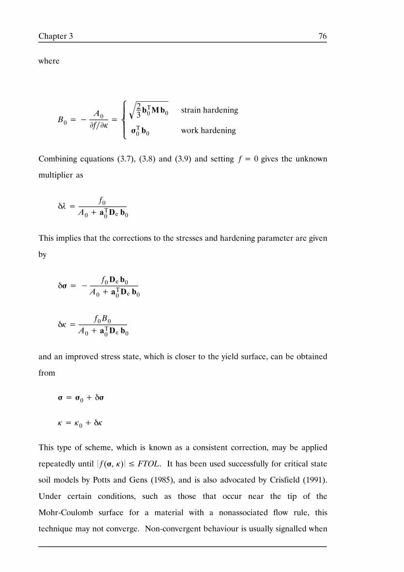
76Chapter 3
where
B0=−A0∂f∕∂À
= ⎪⎪⎨⎧
⎩
23 bT0Mb0
σT0 b0
strain hardening
work hardening
Combining equations (3.7), (3.8) and (3.9) and setting f= 0 gives the unknown
multiplier as
δλ=f0
A0+ aT0De b0
This implies that the corrections to the stresses and hardening parameter are given
by
δσ= −f0De b0
A0+ aT0De b0
δÀ=f0B0
A0+ aT0De b0
and an improved stress state, which is closer to the yield surface, can be obtained
from
σ= σ0+ δσ
À= À0+ δÀ
This type of scheme, which is known as a consistent correction, may be applied
repeatedly until f (σ, À) ≤ FTOL. It has been used successfully for critical state
soil models by Potts and Gens (1985), and is also advocated by Crisfield (1991).
Under certain conditions, such as those that occur near the tip of the
Mohr-Coulomb surface for a material with a nonassociated flow rule, this
technique may not converge. Non-convergent behaviour is usually signalled when
77Chapter 3
the corrected stress state is further from the yield surface than the uncorrected
stress state. In these circumstances, the consistent return scheme may be
abandoned for one iteration and replaced with a correction which is normal to the
yield surface. This method, known as the normal correction, does not preserve
the total applied strain increment, but is very reliable and has been used
successfully by Nayak and Zienkiewicz (1972a), Owen and Hinton (1980), and
Sloan and Randolph (1982). With the normal correction scheme, equation (3.8)
is replaced by
δσ= − δλ a0
and it is assumed that the hardening parameter À0 remains unchanged. Using the
same argument as before, but neglecting any changes in À, it follows that
δσ= −f0 a0aT0 a0
(3.10)
This type of correction may also be applied iteratively until f (σ, À0) ≤ FTOL and
has proven to be very robust in practice.
The complete algorithm for returning the stresses to the yield surface and may be
summarised as follows.
Yield Surface Correction Scheme
1. Enter with uncorrected stresses σ0 and hardening parameter À0.
2. Do steps 3 to 6 MAXITS times.
3. Compute
δλ=f0
A0+ aT0Deb0
and then correct stresses and hardening parameter using
σ= σ0− δλDe b0
À= À0+ δλ B0
78Chapter 3
4. If |f (σ,À)|> |f (σ0,À0)|, then abandon previous correction and
compute
δλ=f0aT0 a0
σ= σ0− δλ a0
À= À0
5. If |f (σ,À)|≤ FTOL, then go to step 8.
6. Set σ0= σ and À0= À
7. Convergence not achieved after MAXITS steps, print error message and
stop.
8. Exit with stresses σ and hardening parameter À lying on the yield surface.
A suitable value for MAXITS, which denotes the maximum number of correction
iterations permitted, is typically between five and ten. Note that this correction
procedure will also be used for the single step backward Euler scheme described
in a later Section.
3.3.4 Modified Euler Scheme with Substepping
For a given strain increment, Δε, the constitutive relations to be integrated at each
Gauss point are described by equations (3.3) and (3.4) as
dσdT= DepΔε= Δσe− ΔλDeb (3.11)
dÀdT= ΔλB (3.12)
where
Δλ=aTDeΔεA+ aTDeb
=aTΔσe
A+ aTDeb
79Chapter 3
B=− A∂f∕∂À
=⎪⎪⎨⎧
⎩
23bTMb
σTb
strain hardening
work hardening
and the pseudo time lies in the range
0≤ T≤ 1
These equations describe a system of ordinary differential equations with known
initial conditions σ= σ0 and À= À0 at the start of the increment where T= 0
and t= t0. A wide variety of explicit methods may be used to integrate these
relations to give the stresses and hardening parameter at the end of the increment
where T= 1.
The approach used in this Thesis is based on the scheme of Sloan (1987). Sloan’s
method is attractive for finite element applications because it controls the errors
in the stresses and hardening parameter which are caused by the approximate
integration of the constitutive law. This error control is achieved by using a local
error measure to automatically subincrement the imposed strain increment Δε.
The local error measure is found by taking the difference between a modified
Euler solution, which is of second order accuracy, and an Euler solution, which
is of first order accuracy, for each subincrement. It thus corresponds to an
estimate of the local truncation error. Once the local error has been computed
for a given step, the size of the next step is determined by extrapolation of the
dominant error term. This means that the size of each subincrement may vary
throughout the integration process, depending on the nonlinearity of the
constitutive relations.
Consider a pseudo time subincrement in the range 0< ΔTn≤ 1 and let the
subscripts n− 1 and n denote quantities evaluated at the pseudo times Tn−1 and
Tn= Tn−1+ ΔTn. In the explicit Euler method, the solution for σ and À at the
end of a pseudo time step ΔTn is found from
80Chapter 3
σn= σn−1+ Δσ1
Àn= Àn−1+ ΔÀ1(3.13)
where
Δσ1= Dep (σn−1 , Àn−1 )Δεn
ΔÀ1= Δλ(σn−1 , Àn−1 ,Δεn)B(σn−1)(3.14)
and
Δεn= ΔTnΔε
A more accurate estimate of the stresses and hardening parameter at the end of
the interval ΔTn can be found using the modified Euler procedure. This gives
σ^n= σn−1+12 (Δσ1+ Δσ2)
À^n= Àn−1+12 (ΔÀ1+ ΔÀ2)
(3.15)
where Δσ1 and ΔÀ1 are computed from the Euler scheme and
Δσ2= Dep (σn−1+ Δσ1 , Àn−1 + ΔÀ1)Δεn
ΔÀ2= Δλ(σn−1 + Δσ1 , Àn−1+ ΔÀ1,Δεn)B(σn−1+ Δσ1)
Since the local truncation error in the Euler and modified Euler solutions is,
respectively, O(ΔT2) and O(ΔT3), the error in σn and Àn can be estimated from
⎪⎪⎨⎧
⎩
σ^n
À^n⎪⎪⎬⎫
⎭−⎪⎪⎨⎧
⎩
σn
Àn⎪⎪⎬⎫
⎭=⎪⎪⎨⎧
⎩
12 (Δσ2− Δσ1)
12 (ΔÀ2− ΔÀ1)
⎪⎪⎬⎫
⎭
Using any convenient norm, this quantity can be used to compute the relative error
measure
81Chapter 3
Rn= 12max Δσ2− Δσ1 σ^n ,ΔÀ2− ΔÀ1
À^n (3.16)
Note that the error in the stresses is treated separately from the error in the
hardening parameter to allow for differences of scale. Following Sloan (1987), the
current strain subincrement is accepted if Rn is not greater than some prescribed
tolerance, STOL, and rejected otherwise. Regardless of whether the subincrement
is accepted or rejected, the next pseudo time step is found from the simple relation
ΔTn+1= q ΔTn (3.17)
where q is chosen so that Rn+1 satisfies the constraint
Rn+1≤ STOL (3.18)
Now, since the local truncation error in the Euler method is O(ΔT2), it follows
from (3.17) that
Rn+1≈ q2Rn
Imposing the constraint (3.18) gives
q≤ STOL∕Rn
The above procedure for determining q is based on local extrapolation of the
dominant error term. Because local extrapolation may become inaccurate for
strongly nonlinear behaviour, it is wise to choose q conservatively to minimise the
number of rejected strain subincrements. Numerical experiments on a wide
variety of plasticity problems suggest that a suitable strategy for computing q is to
set
q= 0.9 STOL∕Rn (3.19)
and also constrain it to lie within the limits
0.1≤ q≤ 1.1 (3.20)
82Chapter 3
so that
0.1ΔTn−1≤ ΔTn≤ 1.1ΔTn−1
The coefficient of 0.9 acts merely as a safety factor, since it usually prevents the
step control mechanism from choosing strain subincrements which just fail to meet
the local error tolerance. Restricting the growth of consecutive strain
subincrements to ten percent also has this effect. Numerical experiments indicate
that increasing the maximum growth factor for consecutive subincrements to one
hundred percent has little influence on the performance of the algorithm.
Relaxing these constraints leads to larger subincrement sizes and hence fewer
strain subincrements overall, but this saving is counteracted by the increased
number of failed subincrements. Two final controls, of lesser importance than the
above refinements, impose a minimum absolute step size, ΔTmin, and prohibit the
step size from growing immediately after a failed subincrement. The first
condition is added merely for robustness, and will not be invoked unless the
constitutive law contains gradient singularities. The second condition ensures that
there are at least two strain subincrements of the same size following a failure,
and is useful for cases where the stress-strain path has sharp changes in curvature.
The integration scheme is started by applying (3.13) and (3.14) with the known
strains Δε , the initial stresses σ0, the initial hardening parameter À0, and an initial
pseudo time step ΔT1. In order to minimise the number of strain subincrements
for each Gauss point, ΔT1 is typically set to unity. If the relative error in the
resulting solution, as defined by equation (3.16), is not greater than the specified
tolerance STOL, then the current subincrement is accepted and the stresses and
hardening parameter are updated using either (3.13) or (3.15). In practice, it is
best to employ the higher order update rather than the lower order update, since
this is the most accurate of the two and has already been calculated. The extra
accuracy of the higher order update also compensates for the fact that (3.16) is
only a local and not a global error indicator. After a successful subincrement, the
83Chapter 3
new stresses and hardening parameter are corrected back to the yield surface using
the procedure described in Section 3.3.3. If the specified error tolerance is not
met, so that Rn> STOL,then the solution is rejected and a smaller step size is
computed using equations (3.19) and (3.20). The stage is then repeated and, if
necessary, the step size is reduced further until a successful subincrement size is
obtained. Regardless of whether the current subincrement is accepted or not, the
size of the next strain subincrement is found using (3.19) and (3.20). In successive
steps, the subincrements may become larger, smaller, or stay the same, depending
on the error that is calculated from equation (3.16). The end of the integration
procedure is reached when the entire increment of strain is applied so that
ΔTn= T= 1
The complete explicit modified Euler algorithm, which includes all of the
refinements described in Sections 3.3.1---3.3.3, may be summarised as follows.
Explicit Modified Euler Algorithm With Substepping
1. Enter with initial stresses σ0, initial hardening parameter À0, the strain
increment for the current step Δε, and the error tolerance for the stresses
STOL.
2. Compute the stress increment Δσe and the trial elastic stress state σe
according to
Δσe= DeΔε
σe= σ0+ Δσe
If f (σe,À0)≤ FTOL then the stress increment is purely elastic, so set
σ1= σe and À1= À0 and go to step 16.
3. If f (σ0,À0)<−FTOL and f (σe,À0)> FTOL then the stress point
undergoes a transition from elastic to plastic behaviour. Compute the
portion of Δσe that causes purely elastic deformation, α, using the modified
regula-falsi intersection scheme of Section 3.3.1 and go to step 5.
84Chapter 3
4. If |f (σ0,À0)|≤ FTOL and f (σe,À0)> FTOL then
Check for a negative plastic multiplier by computing the cosine of the
angle between a and Δσe from
cos θ= aTΔσe a 2 Δσe 2
where a is evaluated at the initial stress state.
If cos θ≥− LTOL then
The stress increment is purely plastic, so set α= 0.
else
Elastic unloading followed by plastic flow occurs. Compute the
portion of Δσe that causes purely elastic deformation, α, using
the modified regula-falsi intersection scheme for negative plastic
multipliers of Section 3.3.2.
else
The stress state is illegal.
5. Update the stresses at the onset of plastic yielding as σ0← σ0+ αΔσe.
Then compute the portion of Δσe that causes plastic deformation according
to Δσe← (1− α)Δσe.
6. Set T=0 and ΔT=1.
7. While T<1, do steps 8 to 15.
8. Compute Δσi and ΔÀi for i = 1 to 2 using
Δσi= ΔTΔσe − ΔλiDebi
ΔÀi= Δλi Bi
where
Δλi= max⎨⎧⎩ΔT aTi ΔσeAi+ aTi De bi
, 0⎬⎫⎭
85Chapter 3
Bi=−Ai∂f∕∂À= ⎪
⎪⎨⎧
⎩
23 bTi Mbi
σTi bi
strain hardening
work hardening
Ai=− (∂f∕∂À)Bi
ai= ∂f∂σi
bi= ∂g∂σi
are evaluated at (σi , Ài ), and
σ1= σT
σ2= σT+ Δσ1
À1= ÀT
À2= ÀT+ ΔÀ1
9. Compute the new stresses and hardening parameter and hold them in
temporary storage according to
σT+ΔT= σT+12 (Δσ1+ Δσ2)
ÀT+ΔT= ÀT+12 (ΔÀ1+ ΔÀ2)
10. Determine the relative error for the current substep from
RT+ΔT= max Δσ2− Δσ1 2 σT+ΔT , ΔÀ2− ΔÀ12ÀT+ΔT
, EPSwhere EPS is a machine constant indicating the smallest relative error
that may be calculated.
11. If RT+ΔT> STOL, then this substep has failed, so extrapolate to
obtain a smaller pseudo time step. First compute
q= max 0.9 STOL∕RT+ΔT , 0.1
and then set
86Chapter 3
ΔT← max { qΔT , ΔTmin }
before returning to step 8.
12. The substep is accepted, so update the stresses and the hardening
parameter according to
σT+ΔT= σT+ΔT
ÀT+ΔT= ÀT+ΔT
13. If f (σT+ΔT ,ÀT+ΔT) > FTOL, then correct σT+ΔT and ÀT+ΔT back
to the yield surface using the algorithm of Section 3.3.3.
14. Extrapolate to obtain the size of the next substep by computing
q= min 0.9 STOL∕RT+ΔT , 1.1
If previous step failed, limit growth of step size further by enforcing
q= min{q , 1}
Compute new step size and update pseudo time according to
ΔT← q ΔT
T← T+ ΔT
15. Ensure that next step size is not smaller than the minimum step size
and check that integration does not proceed beyond T=1 by setting
ΔT← max { ΔT , ΔTmin }
and then
ΔT← min { ΔT , 1− T }
16. Exit with stresses σ1 and hardening parameter À1 at end of increment,
where T=1.
An appropriate value for the tolerance LTOL, which is used for detecting elastic
unloading in step 4, is around 10---6. The tolerance EPS, which is used to define
the minimum relative error in step 10, is typically set to around 10---16 for double
precision arithmetic on a 32-bit machine.
87Chapter 3
The above scheme incorporates a several important refinements to the original
integration scheme of Sloan (1987). These include the improved regula-falsi
method for computing the elastic-plastic transition point on the yield surface, the
new scheme for dealing with negative plastic multipliers which cause plastic flow,
and the consistent yield surface correction procedure. Apart from these
algorithmic changes, a number of ‘tuning’ adjustments have also been made as a
result of extensive numerical experiments. The ‘safety factor’ coefficient on the
subincrement size, which was originally 0.8, has been increased to 0.9 to give better
control of the integration process. To minimise the number of rejected substeps,
the maximum growth in size between successive subincrements has been reduced
from one hundred percent to ten percent and no growth in the step size is now
permitted for the two subincrements that immediately follow a failed step. In the
event that a discontinuous yield surface is employed, a minimum step size has also
been introduced to force the integration of the constitutive equations. Typical
values for the minimum substep size ΔTmin are of the order of 10---4, which implies
that a maximum of 10,000 substeps may be used in the integration process.
3.3.5 Single Step Modified Euler Scheme
A single step modified Euler scheme can be derived from the previous algorithm
merely by setting the integration tolerance, STOL, to a large value. Results from
this type of method will be discussed in a later Section of this Chapter to provide
an indication of the accuracy of explicit integration schemes that do not employ
subincrementation.
3.3.6 Dormand-Prince Scheme with Substepping
The explicit Runge-Kutta-Dormand-Prince scheme is similar to the modified Euler
scheme described above except that a pair of four and fifth order integration
formulae are used to estimate the stresses and hardening parameter (Sloan and
Booker, 1992). With this high order algorithm, the stresses and hardening
parameter computed at the end of each subincrement are very accurate and
88Chapter 3
seldom need to be corrected back to the yield surface to satisfy the yield tolerance
of FTOL=10---9. This type of scheme is useful for checking the accuracy of lower
order methods, as it can be used with a stringent stress tolerance of STOL=10---9
or smaller.
When applied to (3.11) and (3.12) for a pseudo time step ΔTn, the fourth and fifth
order solutions for the stresses and hardening parameters, are given by
σn= σn−1+31540Δσ1+
190297Δσ3−
145108Δσ4+
351220Δσ5+
120Δσ6
Àn= Àn−1+31540ΔÀ1+
190297ΔÀ3−
145108ΔÀ4+
351220ΔÀ5+
120ΔÀ6
(3.21)
and
σ^n= σn−1+19216Δσ1+
10002079Δσ3−
125216Δσ4+
8188Δσ5+
556Δσ6
À^n= Àn−1+19216ΔÀ1+
10002079ΔÀ3−
125216ΔÀ4−
8188ΔÀ5+
556ΔÀ6
(3.22)
where
Δσi= Dep(σi, Ài)Δεn
ΔÀi= Δλ(σi, Ài,Δεn)B(σi)⎪⎪⎬⎫
⎭for i= 1, 2,. . ., 6
Δεn= ΔTn Δε
and
σ1= σn−1
À1= Àn−1(3.23)
89Chapter 3
σ2= σn−1+15Δσ1
À2= Àn−1+15ΔÀ1
(3.24)
σ3= σn−1+340Δσ1+
940Δσ2
À3= Àn−1+340ΔÀ1+
940ΔÀ2
(3.25)
σ4= σn−1+310Δσ1−
910Δσ2+
65Δσ3
À4= Àn−1+310ΔÀ1−
910ΔÀ2+
65ΔÀ3
(3.26)
σ5= σn−1+226729Δσ1−
2527Δσ2+
880729Δσ3+
55729Δσ4
À5= Àn−1+226729ΔÀ1−
2527ΔÀ2+
880729ΔÀ3+
55729ΔÀ4
(3.27)
σ6= σn−1−181270Δσ1+
52Δσ2−
266297Δσ3−
9127Δσ4+
18955Δσ5
À6= Àn−1−181270ΔÀ1+
52ΔÀ2−
266297ΔÀ3+
9127ΔÀ4+
18955 ΔÀ5
(3.28)
Subtracting equations (3.21) from equations (3.22) gives a fifth order estimate of
the local truncation error according to
⎪⎪⎨⎧
⎩
σ^n
À^n⎪⎪⎬⎫
⎭−⎪⎪⎨⎧
⎩
σn
Àn⎪⎪⎬⎫
⎭=⎪⎪⎨⎧
⎩
11360Δσ1−
1063Δσ3+
5572Δσ4−
2740Δσ5+
11280Δσ6
11360ΔÀ1−
1063ΔÀ3+
5572ΔÀ4−
2740ΔÀ5+
11280ΔÀ6
⎪⎪⎬⎫
⎭
The theory for implementing the explicit Dormand-Prince formulae is identical to
that for the modified Euler scheme. Steps 8, 9, 10, 11, and 14 of the algorithm
of Section 3.3.4 need to be changed as follows:
8. The variable i ranges from 1 to 6 and σi and Ài are given by equations
(3.23)---(3.28).
90Chapter 3
9. Compute the new stresses and hardening parameter and hold them in
temporary storage according to
σT+ΔT= σT+19216Δσ1+
10002079Δσ3−
125216Δσ4+
8188Δσ5
ÀT+ΔT= ÀT+19216ΔÀ1+
10002079ΔÀ3−
125216ΔÀ4−
8188ΔÀ5
10. Determine the relative error for the current substep from
RT+ΔT= max⎨⎧⎩ E σT+ΔT
σT+ΔT , E ÀT+ΔT
ÀT+ΔT, EPS⎬⎫⎭
where
E σT+ΔT
= 11360Δσ1−
1063Δσ3+
5572Δσ4−
2740Δσ5+
11280Δ
E ÀT+ΔT
= 11360ΔÀ1−
1063ΔÀ3+
5572ΔÀ4−
2740ΔÀ5+
11280Δ
and EPS is a machine constant indicating the smallest relative error
that may be calculated.
11. If RT+ΔT> STOL, then this substep has failed, so extrapolate to
obtain a smaller pseudo time step. First compute
q= max 0.9(STOL∕RT+ΔT)1∕5 , 0.1
and then set
ΔT← max { qΔT , ΔTmin }
before returning to step 8.
14. Extrapolate to obtain the size of the next substep by computing
q= min 0.9(STOL∕RT+ΔT)1∕5 , 1.1
If previous step failed, limit growth of step size further by enforcing
q= min{q , 1}
91Chapter 3
Compute new step size and update pseudo time according to
ΔT← q ΔT
T← T+ ΔT
The extra accuracy of the Dormand-Prince scheme is obtained at the expense of
additional evaluations of the constitutive relations for each subincrement. Six
evaluations per subincrement are needed, as opposed to two for the modified
Euler algorithm.
3.4 IMPLICIT INTEGRATION SCHEMES
A comprehensive discussion of various implicit stress integration methods has been
given by Crisfield (1991). Two schemes that have found wide application in metal
plasticity codes are forms of the backward Euler algorithm. The first of these,
which is termed a single step backward Euler method, is simple to implement since
it does not require second derivatives of the yield function or plastic potential.
The second method uses the well known backward Euler scheme for solving a
system of first order differential equations.
3.4.1 Single Step Backward Euler Scheme
The single step backward Euler scheme begins by computing the same trial elastic
stress state as before according to the sequence
Δε= BΔu
Δσe= DeΔε
σe= σ0+ Δσe
The stresses σe are then returned to the yield surface by using a single backward
Euler return and, if necessary, the correction process described in Section 3.3.3.
To derive the backward Euler return, f is expanded in a truncated Taylor series
about σe to give
92Chapter 3
f= fe+ aTe Δσ+∂f∂ÀΔÀ (3.29)
where Δσ is the elastoplastic stress increment, ΔÀ is the hardening parameter
increment, fe= f (σe , À0), and ae is evaluated at σe. In returning the stress state
to the yield surface, the total strain increment, Δε, must remain unchanged since
all of it has already been applied in computing the stress σe. Inspection of
equation (2.5) reveals that this condition is satisfied if the stress increment obeys
the relation
Δσ= − ΔλDe be (3.30)
where Δλ is an unknown multiplier and be is evaluated at σe. Using (3.2), the
hardening correction may be expressed as
ΔÀ= Δλ Be (3.31)
where
Be=−Ae∂f∕∂À= ⎪
⎪⎨⎧
⎩
23 bTeMbe
σTe be
strain hardening
work hardening
Substituting (3.30) and (3.31) in (3.29) and setting f= f (σ , À)= 0 gives the
unknown multiplier as
Δλ=fe
Ae+ aTe De be
This implies that the updated stresses and hardening parameter are
σ1= σe− ΔλDebe
À1= À0+ Δλ Be
If this updated stress state lies off the yield surface, so that f (σ1 , À1) > FTOL,
the correction algorithm of Section 3.3.3 is applied until f (σ1 , À1) ≤ FTOL. The
complete single step backward Euler procedure is described below.
93Chapter 3
Single Step Backward Euler Algorithm
1. Enter with initial stresses σ0, initial hardening parameter À0, and the
current strain increment Δε.
2. Compute the elastic stress increment Δσe and the trial elastic stress state
σe according to
Δσe= DeΔε
σe= σ0+ Δσe
If f (σe ,À0)≤ FTOL, then the increment is elastic so set σ1= σe and
À1= À0 and go to step 5.
3. Compute the plastic multiplier
Δλ=f (σe , À0)Ae+ aTe De be
and then update the stresses and hardening parameter using
σ1= σe− ΔλDe be
À1= À0+ Δλ Be
4. If f (σ1 ,À1) > FTOL, then restore stress state to yield surface using
algorithm of Section 3.3.3.
5. Exit with updated stresses σ1 and hardening parameter À1.
Note that the single step backward Euler method does not require the yield
surface intersection point to be found if the stress point undergoes a transition
from elastic to elastoplastic behaviour. This feature is an advantage over the
explicit schemes described previously. In cases where the strain increment is large
and the trial stress point, σe, is a long way outside the yield surface, the first
backward Euler return step may give a stress state for which f (σ1 ,À1)&FTOL.
Restoring the stress state to the yield surface then becomes vital and can cause
problems for complex constitutive models in which the gradients vary rapidly.
94Chapter 3
3.4.2 Backward Euler Return Scheme
The backward Euler return scheme involves solving a small system of nonlinear
equations at each Gauss point. These equations correspond to the incremental
form of the elastoplastic constitutive relations which, from (2.5), may be written
as
Δσ= Δσe− ΔλDeb
Letting σ0 denote the initial stress state, σe= σ0+ Δσe the trial elastic stress
state, and σ the final stress state, these equations may also be expressed in the
form
σ− σ0= σe− σ0− ΔλDe b
or
σ= σe− ΔλDeb
These equations are nonlinear because b is a function of the stresses and Δλ is
a function of both the stresses and the hardening parameter. To solve these
equations iteratively, it is convenient to define the residual
r= σ− σe+ ΔλDeb
which indicates how well the constitutive relations are satisfied at the current
values of σ and À. Noting that σe is constant and expanding r in a truncated Taylor
series gives
r= r0+∂σ∂σ δσ+ Δλ0De∂b∂σ0δσ+
∂(Δλ)∂(Δλ)
Deb0 δλ
where
r0= σ0− σe+ Δλ0Deb0
In the above, δσ is the iterative change in the elastoplastic stress increment, δλ
is the iterative change in the plastic multiplier, and the subscript 0 indicates
95Chapter 3
quantities that are evaluated using the stresses and hardening parameter at the
start of the iteration. Setting r= 0 and collecting terms, the iterative stress
increment is obtained as
δσ=−Q−10 r0+ δλDeb0 (3.32)
where
Q0= I+ Δλ0De∂b∂σ0and I is the identity matrix. To obtain the iterative change in the plastic multiplier,
δλ, the yield function f is expanded in a truncated Taylor series about the current
stress point according to
f= f0+ aT0 δσ+
∂f∂À δÀ= f0+ a
T0 δσ− A0δλ
where
δÀ= δλB0 (3.33)
and
B0=−A0∂f∕∂À
= ⎪⎪⎨⎧
⎩
23 bT0Mb0
σT0 b0
strain hardening
work hardening
Setting f= 0 and substituting (3.32) gives
δλ=f0− aT0 Q
−10 r0
A0+ aT0 Q−10 De b0
(3.34)
Equations (3.32)---(3.34) define the iterative change in the elastoplastic stress
increment and the hardening parameter. The stress state at the end of the
iteration is obtained from
96Chapter 3
σ= σ0+ δσ
À= À0+ δÀ
and the iterations are continued until f (σ ,À) ≤ FTOL.
As with the single step backward Euler method, the backward Euler return scheme
does not require the transition point between elastic and elastoplastic behaviour
to be isolated. This advantage is somewhat nullified by the fact that the gradient
derivative ∂b∕∂σ, which is needed to form the matrix Q, is often cumbersome to
enumerate for complex constitutive laws.
It should be noted that convergence of the backward Euler return scheme is not
guaranteed, particularly for large strain increments. To overcome this drawback,
it is advisable to implement a simple substepping strategy which automatically cuts
the size of the imposed strain increment if the stress state starts to diverge from
the yield surface between successive iterations. As a further safeguard, the strain
increment should also be reduced if convergence has not occurred within a
specified number of iterations.
The algorithm for the backward Euler return scheme, with substepping, is
summarised below.
Backward Euler Return Scheme
1. Enter with initial stresses σ0, initial hardening parameter À0, and the
current strain increment Δε.
2. Compute the elastic stress increment Δσe according to
Δσe= DeΔε
3. Set T=0 and ΔT=1.
4. While T<1, do steps 5---7 and steps 12---14 (substepping loop).
5. Compute
97Chapter 3
σe= σT+ ΔσeΔT
If f (σe,ÀT)≤ FTOL, then set σT+ΔT= σe and ÀT+ΔT= ÀT and go
to step 13.
6. First compute the multiplier
Δλ0T+ΔT=f (σe , ÀT)Ae+ aTe De be
Then set starting values for stresses and hardening parameter
according to
σ0T+ΔT= σe− Δλ0T+ΔTDe be
À0T+ΔT= ÀT+ Δλ0T+ΔT Be
If f (σ0T+ΔT , À0T+ΔT) ≤ FTOL, then set σT+ΔT= σ0T+ΔT and
ÀT+ΔT= À0T+ΔT and go to step 13.
7. Do steps 8 to 11 for i=1 to MAXITS (iteration loop).
8. Compute
δλi=f (σ i−1T+ΔT
, À i−1T+ΔT
)− aTsA+ aT t
where
s= Q–1 (σ i−1T+ΔT
− σe+ Δλi−1T+ΔTDeb)
t= Q–1Deb
Q= I+ Δλi−1T+ΔTDe ∂b∂σand A, a, b, and ∂b∕∂σ are all evaluated at (σ i−1
T+ΔT,À i−1T+ΔT
).
Then compute the iterative change in the stresses and hardening
parameter using
δσ i=− s− δλi t
δÀ i= δλi B
98Chapter 3
9. If f (σ i−1T+ΔT
+ δσ i,À i−1T+ΔT
+ δÀ i) > f(σ i−1T+ΔT
,À i−1T+ΔT
) , then goto step 12.
10. Update stresses, hardening parameter, and plastic multiplier
according to
σ iT+ΔT
= σ i−1T+ΔT
+ δσ i
À iT+ΔT
= À i−1T+ΔT
+ δÀ i
ΔλiT+ΔT= Δλi−1T+ΔT+ δλ
i
11. If |f (σ iT+ΔT
,À iT+ΔT
)|≤ FTOL, then set σT+ΔT= σiT+ΔT and
ÀT+ΔT= ÀiT+ΔT and go to step 13.
12. This substep failed to converge. Calculate new substep size according
to
ΔT← ΔT∕2
and return to step 5.
13. Check that the integration does not proceed beyond T=1 by setting
ΔT← min { ΔT , 1− T }
14. Update pseudo time according to
T← T+ ΔT
15. Exit with updated stresses σ1 and hardening parameter À1.
A typical value for the maximum number of backward Euler iterations, MAXITS,
is around five. If this limit is exceeded, the above scheme repeatedly halves the
applied strain increment until successful convergence is achieved.
3.5 COMPARISON OF INTEGRATION SCHEMES
To compare their numerical performance, each of the integration schemes
described in Sections 3.3 and 3.4 is used to predict the behaviour of a smooth rigid
strip footing resting on an elastoplastic soil mass. Due to the singularity at the
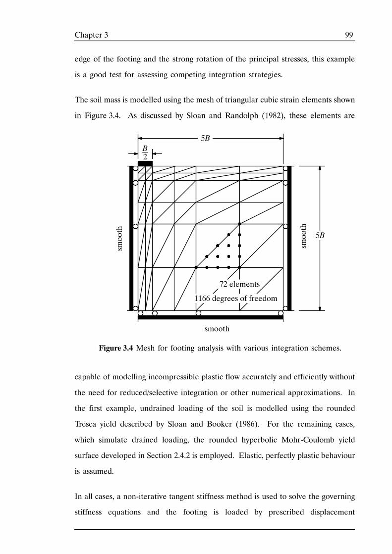
99Chapter 3
edge of the footing and the strong rotation of the principal stresses, this example
is a good test for assessing competing integration strategies.
The soil mass is modelled using the mesh of triangular cubic strain elements shown
in Figure 3.4. As discussed by Sloan and Randolph (1982), these elements are
smooth
smooth
smooth
B2
Figure 3.4 Mesh for footing analysis with various integration schemes.
5B
5B
72 elements
1166 degrees of freedom
capable of modelling incompressible plastic flow accurately and efficiently without
the need for reduced/selective integration or other numerical approximations. In
the first example, undrained loading of the soil is modelled using the rounded
Tresca yield described by Sloan and Booker (1986). For the remaining cases,
which simulate drained loading, the rounded hyperbolic Mohr-Coulomb yield
surface developed in Section 2.4.2 is employed. Elastic, perfectly plastic behaviour
is assumed.
In all cases, a non-iterative tangent stiffness method is used to solve the governing
stiffness equations and the footing is loaded by prescribed displacement
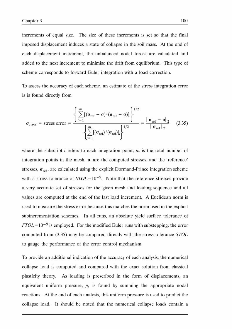
100Chapter 3
increments of equal size. The size of these increments is set so that the final
imposed displacement induces a state of collapse in the soil mass. At the end of
each displacement increment, the unbalanced nodal forces are calculated and
added to the next increment to minimise the drift from equilibrium. This type of
scheme corresponds to forward Euler integration with a load correction.
To assess the accuracy of each scheme, an estimate of the stress integration error
is is found directly from
σerror= stress error=
⎨⎧⎩mi=1[(σref− σ)T(σref− σ)]i⎬
⎫⎭1∕2
⎨⎧⎩mi=1[(σref)T(σref)]i⎬
⎫⎭1∕2
= σref− σ 2 σref 2
(3.35)
where the subscript i refers to each integration point, m is the total number of
integration points in the mesh, σ are the computed stresses, and the ‘reference’
stresses, σref , are calculated using the explicit Dormand-Prince integration scheme
with a stress tolerance of STOL=10---9. Note that the reference stresses provide
a very accurate set of stresses for the given mesh and loading sequence and all
values are computed at the end of the last load increment. A Euclidean norm is
used to measure the stress error because this matches the norm used in the explicit
subincrementation schemes. In all runs, an absolute yield surface tolerance of
FTOL=10---9 is employed. For the modified Euler runs with substepping, the error
computed from (3.35) may be compared directly with the stress tolerance STOL
to gauge the performance of the error control mechanism.
To provide an additional indication of the accuracy of each analysis, the numerical
collapse load is computed and compared with the exact solution from classical
plasticity theory. As loading is prescribed in the form of displacements, an
equivalent uniform pressure, p, is found by summing the appropriate nodal
reactions. At the end of each analysis, this uniform pressure is used to predict the
collapse load. It should be noted that the numerical collapse loads contain a
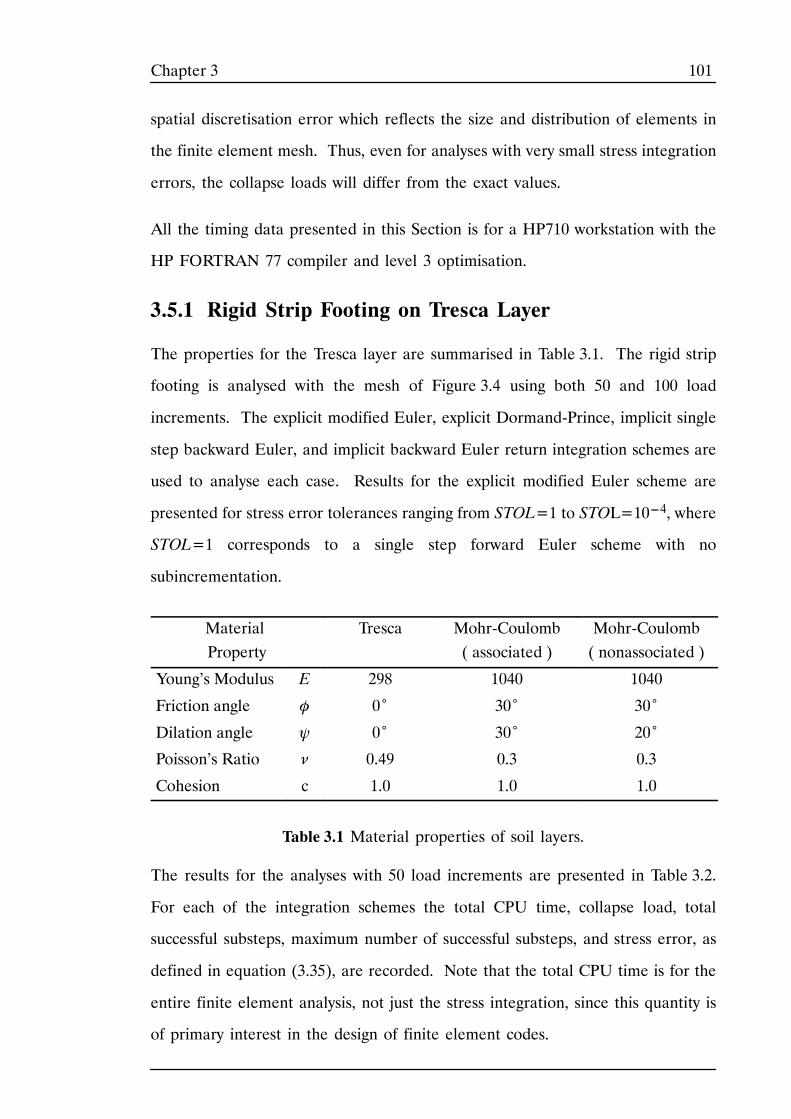
101Chapter 3
spatial discretisation error which reflects the size and distribution of elements in
the finite element mesh. Thus, even for analyses with very small stress integration
errors, the collapse loads will differ from the exact values.
All the timing data presented in this Section is for a HP710 workstation with the
HP FORTRAN 77 compiler and level 3 optimisation.
3.5.1 Rigid Strip Footing on Tresca Layer
The properties for the Tresca layer are summarised in Table 3.1. The rigid strip
footing is analysed with the mesh of Figure 3.4 using both 50 and 100 load
increments. The explicit modified Euler, explicit Dormand-Prince, implicit single
step backward Euler, and implicit backward Euler return integration schemes are
used to analyse each case. Results for the explicit modified Euler scheme are
presented for stress error tolerances ranging from STOL=1 to STOL=10---4, where
STOL=1 corresponds to a single step forward Euler scheme with no
subincrementation.
MaterialProperty
Tresca Mohr-Coulomb( associated )
Mohr-Coulomb( nonassociated )
Young’s Modulus E 298 1040 1040
Friction angle φ 0˚ 30˚ 30˚
Dilation angle ψ 0˚ 30˚ 20˚
Poisson’s Ratio ν 0.49 0.3 0.3
Cohesion c 1.0 1.0 1.0
Table 3.1 Material properties of soil layers.
The results for the analyses with 50 load increments are presented in Table 3.2.
For each of the integration schemes the total CPU time, collapse load, total
successful substeps, maximum number of successful substeps, and stress error, as
defined in equation (3.35), are recorded. Note that the total CPU time is for the
entire finite element analysis, not just the stress integration, since this quantity is
of primary interest in the design of finite element codes.
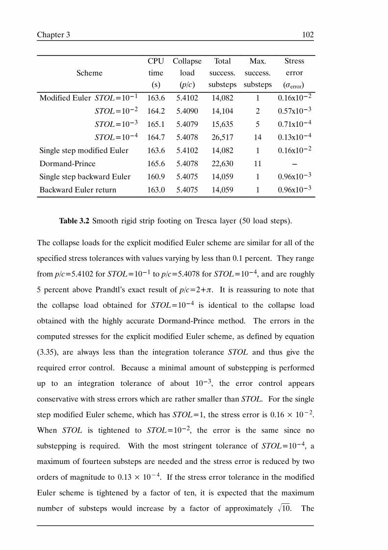
102Chapter 3
SchemeCPUtime(s)
Collapseload(p/c)
Totalsuccess.substeps
Max.success.substeps
Stresserror(σerror)
Modified Euler STOL=10---1 163.6 5.4102 14,082 1 0.16x10---2
STOL=10---2 164.2 5.4090 14,104 2 0.57x10---3
STOL=10---3 165.1 5.4079 15,635 5 0.71x10---4
STOL=10---4 164.7 5.4078 26,517 14 0.13x10---4
Single step modified Euler 163.6 5.4102 14,082 1 0.16x10---2
Dormand-Prince 165.6 5.4078 22,630 11 ---
Single step backward Euler 160.9 5.4075 14,059 1 0.96x10---3
Backward Euler return 163.0 5.4075 14,059 1 0.96x10---3
Table 3.2 Smooth rigid strip footing on Tresca layer (50 load steps).
The collapse loads for the explicit modified Euler scheme are similar for all of the
specified stress tolerances with values varying by less than 0.1 percent. They range
from p/c=5.4102 for STOL=10---1 to p/c=5.4078 for STOL=10---4, and are roughly
5 percent above Prandtl’s exact result of p/c=2+π. It is reassuring to note that
the collapse load obtained for STOL=10---4 is identical to the collapse load
obtained with the highly accurate Dormand-Prince method. The errors in the
computed stresses for the explicit modified Euler scheme, as defined by equation
(3.35), are always less than the integration tolerance STOL and thus give the
required error control. Because a minimal amount of substepping is performed
up to an integration tolerance of about 10---3, the error control appears
conservative with stress errors which are rather smaller than STOL. For the single
step modified Euler scheme, which has STOL=1, the stress error is 0.16× 10⁻².
When STOL is tightened to STOL=10---2, the error is the same since no
substepping is required. With the most stringent tolerance of STOL=10---4, a
maximum of fourteen substeps are needed and the stress error is reduced by two
orders of magnitude to 0.13× 10⁻⁴. If the stress error tolerance in the modified
Euler scheme is tightened by a factor of ten, it is expected that the maximum
number of substeps would increase by a factor of approximately 10 . The
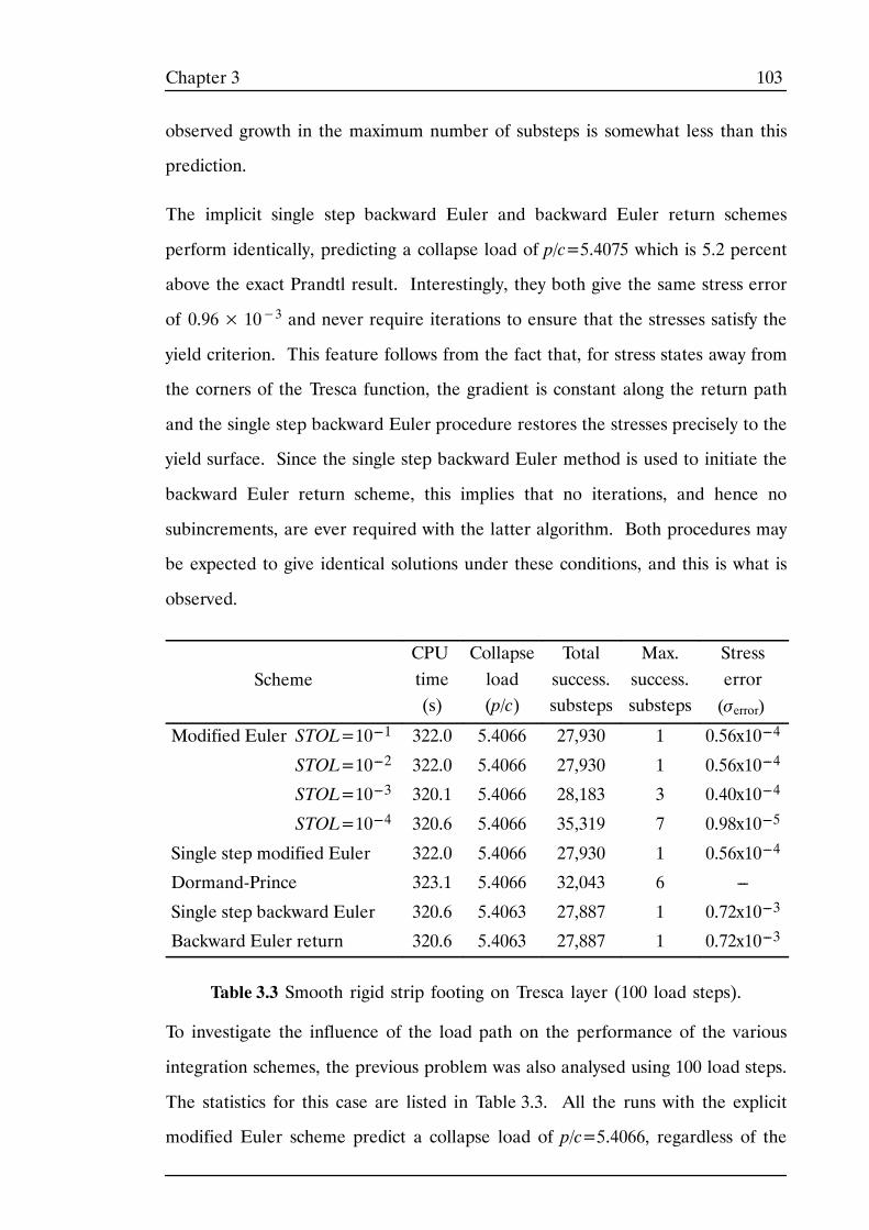
103Chapter 3
observed growth in the maximum number of substeps is somewhat less than this
prediction.
The implicit single step backward Euler and backward Euler return schemes
perform identically, predicting a collapse load of p/c=5.4075 which is 5.2 percent
above the exact Prandtl result. Interestingly, they both give the same stress error
of 0.96× 10⁻³ and never require iterations to ensure that the stresses satisfy the
yield criterion. This feature follows from the fact that, for stress states away from
the corners of the Tresca function, the gradient is constant along the return path
and the single step backward Euler procedure restores the stresses precisely to the
yield surface. Since the single step backward Euler method is used to initiate the
backward Euler return scheme, this implies that no iterations, and hence no
subincrements, are ever required with the latter algorithm. Both procedures may
be expected to give identical solutions under these conditions, and this is what is
observed.
SchemeCPUtime(s)
Collapseload(p/c)
Totalsuccess.substeps
Max.success.substeps
Stresserror(σerror)
Modified Euler STOL=10---1 322.0 5.4066 27,930 1 0.56x10---4
STOL=10---2 322.0 5.4066 27,930 1 0.56x10---4
STOL=10---3 320.1 5.4066 28,183 3 0.40x10---4
STOL=10---4 320.6 5.4066 35,319 7 0.98x10---5
Single step modified Euler 322.0 5.4066 27,930 1 0.56x10---4
Dormand-Prince 323.1 5.4066 32,043 6 ---
Single step backward Euler 320.6 5.4063 27,887 1 0.72x10---3
Backward Euler return 320.6 5.4063 27,887 1 0.72x10---3
Table 3.3 Smooth rigid strip footing on Tresca layer (100 load steps).
To investigate the influence of the load path on the performance of the various
integration schemes, the previous problem was also analysed using 100 load steps.
The statistics for this case are listed in Table 3.3. All the runs with the explicit
modified Euler scheme predict a collapse load of p/c=5.4066, regardless of the
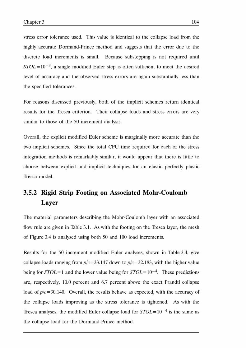
104Chapter 3
stress error tolerance used. This value is identical to the collapse load from the
highly accurate Dormand-Prince method and suggests that the error due to the
discrete load increments is small. Because substepping is not required until
STOL=10---3, a single modified Euler step is often sufficient to meet the desired
level of accuracy and the observed stress errors are again substantially less than
the specified tolerances.
For reasons discussed previously, both of the implicit schemes return identical
results for the Tresca criterion. Their collapse loads and stress errors are very
similar to those of the 50 increment analysis.
Overall, the explicit modified Euler scheme is marginally more accurate than the
two implicit schemes. Since the total CPU time required for each of the stress
integration methods is remarkably similar, it would appear that there is little to
choose between explicit and implicit techniques for an elastic perfectly plastic
Tresca model.
3.5.2 Rigid Strip Footing on Associated Mohr-Coulomb
Layer
The material parameters describing the Mohr-Coulomb layer with an associated
flow rule are given in Table 3.1. As with the footing on the Tresca layer, the mesh
of Figure 3.4 is analysed using both 50 and 100 load increments.
Results for the 50 increment modified Euler analyses, shown in Table 3.4, give
collapse loads ranging from p/c=33.147 down to p/c=32.183, with the higher value
being for STOL=1 and the lower value being for STOL=10---4. These predictions
are, respectively, 10.0 percent and 6.7 percent above the exact Prandtl collapse
load of p/c=30.140. Overall, the results behave as expected, with the accuracy of
the collapse loads improving as the stress tolerance is tightened. As with the
Tresca analyses, the modified Euler collapse load for STOL=10---4 is the same as
the collapse load for the Dormand-Prince method.

105Chapter 3
SchemeCPUtime(s)
Collapseload(p/c)
Totalsuccess.substeps
Max.success.substeps
Stresserror(σerror)
Modified Euler STOL=10---1 168.2 32.582 26,541 20 0.52x10---1
STOL=10---2 169.0 32.242 28,725 91 0.17x10---1
STOL=10---3 169.9 32.185 40,556 280 0.21x10---2
STOL=10---4 174.2 32.183 78,819 290 0.20x10---3
Single step modified Euler 169.3 33.147 25,360 1 0.91x10---1
Dormand-Prince 180.2 32.183 66,575 166 ---
Single step backward Euler 166.5 32.957 25,288 1 0.69x10---1
Backward Euler return 173.0 32.175 28,484 256 0.27x10---2
Table 3.4 Smooth rigid strip footing on associated Mohr-Coulomb layer(50 load steps).
The observed stress errors for the explicit modified Euler scheme are always close
to the specified stress tolerance STOL. Indeed, the stress errors are generally
within an order of magnitude of the required levels, and thus display a ‘tolerance
proportionality’ which is certainly sufficient for controlling the stress integration
error in practical finite element analysis. For example, the most accurate modified
Euler integration, with STOL=10---4, gives a stress error of 2.0× 10⁻⁴, while
analysis with STOL=10---1 gives an error of 0.52× 10⁻¹. Compared with the
corresponding results for the Tresca soil model, the Mohr-Coulomb stress-strain
relations typically require more than twice the total number of substeps to achieve
the same level of accuracy.
Generally speaking, the explicit and implicit single step integration schemes
perform in a like manner. The stress errors for these two methods are,
respectively, 0.91× 10⁻¹ and 0.69× 10⁻¹ and they both give similar collapse
loads. The stress error and collapse load for the backward Euler return scheme
indicate that it is significantly more accurate than the single step backward Euler
approach. Because the gradients along the return path are constant for the
Mohr-Coulomb relations, both versions of the backward Euler method do not
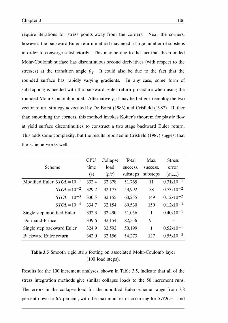
106Chapter 3
require iterations for stress points away from the corners. Near the corners,
however, the backward Euler return method may need a large number of substeps
in order to converge satisfactorily. This may be due to the fact that the rounded
Mohr-Coulomb surface has discontinuous second derivatives (with respect to the
stresses) at the transition angle θT. It could also be due to the fact that the
rounded surface has rapidly varying gradients. In any case, some form of
substepping is needed with the backward Euler return procedure when using the
rounded Mohr-Coulomb model. Alternatively, it may be better to employ the two
vector return strategy advocated by De Borst (1986) and Crisfield (1987). Rather
than smoothing the corners, this method invokes Koiter’s theorem for plastic flow
at yield surface discontinuities to construct a two stage backward Euler return.
This adds some complexity, but the results reported in Crisfield (1987) suggest that
the scheme works well.
SchemeCPUtime(s)
Collapseload(p/c)
Totalsuccess.substeps
Max.success.substeps
Stresserror(σerror)
Modified Euler STOL=10---1 332.4 32.378 51,765 11 0.31x10---1
STOL=10---2 329.2 32.175 53,992 58 0.73x10---2
STOL=10---3 330.5 32.155 60,255 149 0.12x10---2
STOL=10---4 334.7 32.154 89,530 150 0.12x10---3
Single step modified Euler 332.3 32.490 51,056 1 0.40x10---1
Dormand-Prince 339.6 32.154 82,556 95 ---
Single step backward Euler 324.9 32.592 50,199 1 0.52x10---1
Backward Euler return 342.0 32.156 54,273 127 0.55x10---3
Table 3.5 Smooth rigid strip footing on associated Mohr-Coulomb layer(100 load steps).
Results for the 100 increment analyses, shown in Table 3.5, indicate that all of the
stress integration methods give similar collapse loads to the 50 increment runs.
The errors in the collapse load for the modified Euler scheme range from 7.8
percent down to 6.7 percent, with the maximum error occurring for STOL=1 and
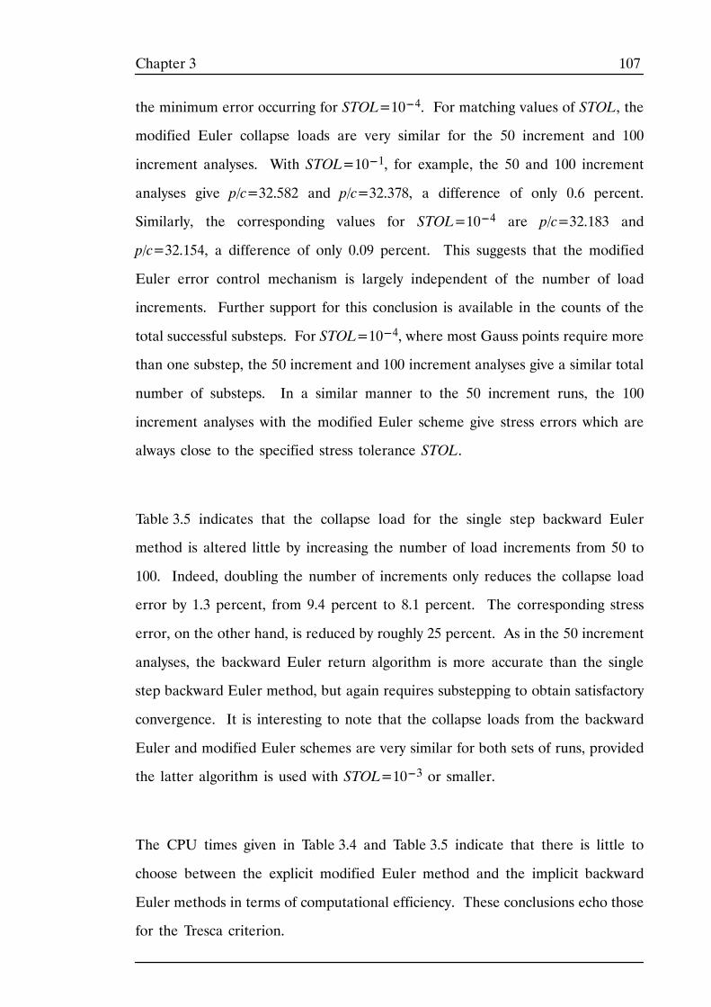
107Chapter 3
the minimum error occurring for STOL=10---4. For matching values of STOL, the
modified Euler collapse loads are very similar for the 50 increment and 100
increment analyses. With STOL=10---1, for example, the 50 and 100 increment
analyses give p/c=32.582 and p/c=32.378, a difference of only 0.6 percent.
Similarly, the corresponding values for STOL=10---4 are p/c=32.183 and
p/c=32.154, a difference of only 0.09 percent. This suggests that the modified
Euler error control mechanism is largely independent of the number of load
increments. Further support for this conclusion is available in the counts of the
total successful substeps. For STOL=10---4, where most Gauss points require more
than one substep, the 50 increment and 100 increment analyses give a similar total
number of substeps. In a similar manner to the 50 increment runs, the 100
increment analyses with the modified Euler scheme give stress errors which are
always close to the specified stress tolerance STOL.
Table 3.5 indicates that the collapse load for the single step backward Euler
method is altered little by increasing the number of load increments from 50 to
100. Indeed, doubling the number of increments only reduces the collapse load
error by 1.3 percent, from 9.4 percent to 8.1 percent. The corresponding stress
error, on the other hand, is reduced by roughly 25 percent. As in the 50 increment
analyses, the backward Euler return algorithm is more accurate than the single
step backward Euler method, but again requires substepping to obtain satisfactory
convergence. It is interesting to note that the collapse loads from the backward
Euler and modified Euler schemes are very similar for both sets of runs, provided
the latter algorithm is used with STOL=10---3 or smaller.
The CPU times given in Table 3.4 and Table 3.5 indicate that there is little to
choose between the explicit modified Euler method and the implicit backward
Euler methods in terms of computational efficiency. These conclusions echo those
for the Tresca criterion.
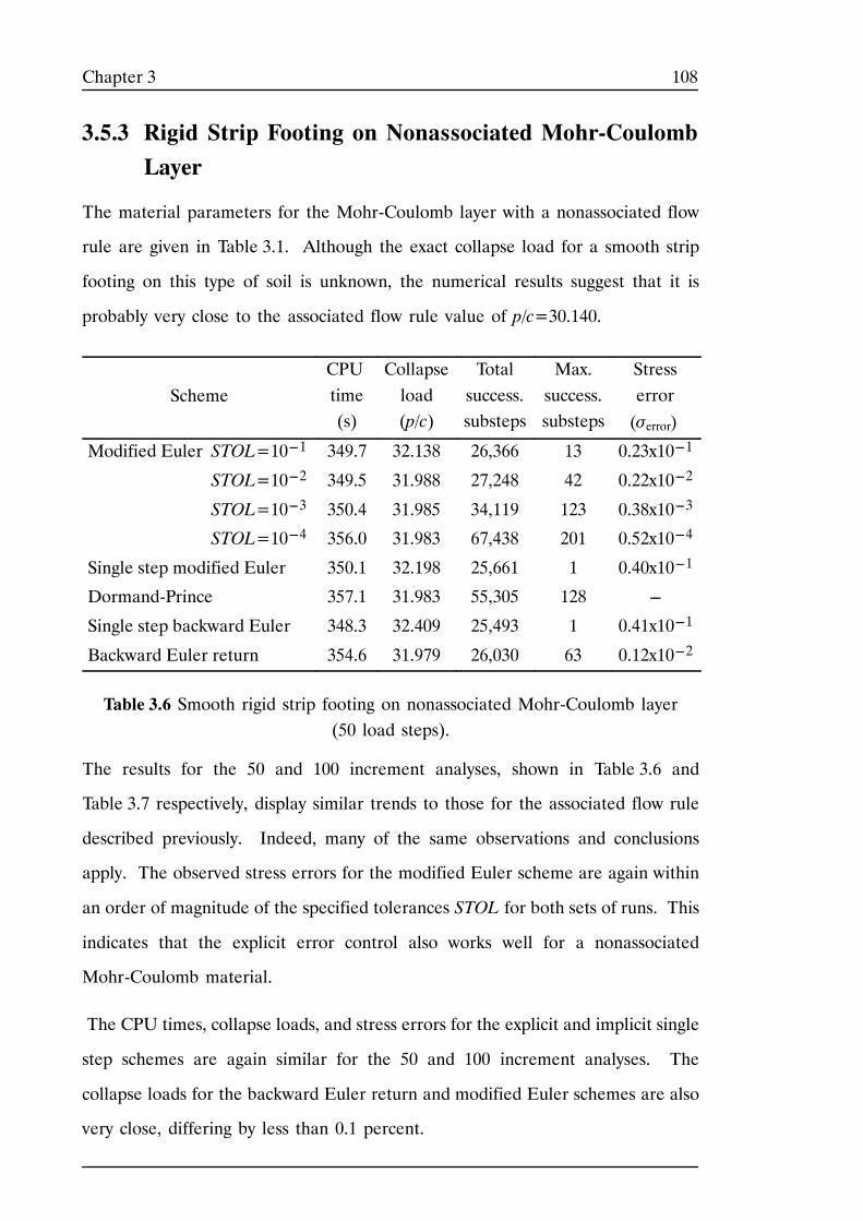
108Chapter 3
3.5.3 Rigid Strip Footing on Nonassociated Mohr-CoulombLayer
The material parameters for the Mohr-Coulomb layer with a nonassociated flow
rule are given in Table 3.1. Although the exact collapse load for a smooth strip
footing on this type of soil is unknown, the numerical results suggest that it is
probably very close to the associated flow rule value of p/c=30.140.
SchemeCPUtime(s)
Collapseload(p/c)
Totalsuccess.substeps
Max.success.substeps
Stresserror(σerror)
Modified Euler STOL=10---1 349.7 32.138 26,366 13 0.23x10---1
STOL=10---2 349.5 31.988 27,248 42 0.22x10---2
STOL=10---3 350.4 31.985 34,119 123 0.38x10---3
STOL=10---4 356.0 31.983 67,438 201 0.52x10---4
Single step modified Euler 350.1 32.198 25,661 1 0.40x10---1
Dormand-Prince 357.1 31.983 55,305 128 ---
Single step backward Euler 348.3 32.409 25,493 1 0.41x10---1
Backward Euler return 354.6 31.979 26,030 63 0.12x10---2
Table 3.6 Smooth rigid strip footing on nonassociated Mohr-Coulomb layer(50 load steps).
The results for the 50 and 100 increment analyses, shown in Table 3.6 and
Table 3.7 respectively, display similar trends to those for the associated flow rule
described previously. Indeed, many of the same observations and conclusions
apply. The observed stress errors for the modified Euler scheme are again within
an order of magnitude of the specified tolerances STOL for both sets of runs. This
indicates that the explicit error control also works well for a nonassociated
Mohr-Coulomb material.
The CPU times, collapse loads, and stress errors for the explicit and implicit single
step schemes are again similar for the 50 and 100 increment analyses. The
collapse loads for the backward Euler return and modified Euler schemes are also
very close, differing by less than 0.1 percent.
109Chapter 3
SchemeCPUtime(s)
Collapseload(p/c)
Totalsuccess.substeps
Maxsuccess.substeps
Stresserror(σerror)
Modified Euler STOL=10---1 692.3 32.079 51,715 7 0.16x10---1
STOL=10---2 694.5 31.976 52,454 21 0.41x10---2
STOL=10---3 693.0 31.954 55,539 100 0.77x10---3
STOL=10---4 695.0 31.951 80,145 108 0.79x10---4
Single step modified Euler 694.2 32.138 51,153 1 0.30x10---1
Dormand-Prince 698.6 31.951 72,214 75 ---
Single step backward Euler 689.2 32.252 50,671 1 0.31x10---1
Backward Euler return 698.8 31.948 51,764 64 0.60x10---3
Table 3.7 Smooth rigid strip footing on nonassociated Mohr-Coulomb layer(100 load steps).
3.6 CONCLUSIONS
The explicit modified Euler and implicit backward Euler return schemes both
provide an economical means of integrating rounded forms of the Tresca and
Mohr-Coulomb constitutive laws. Each procedure requires a similar amount of
CPU time and gives stresses which are of a similar accuracy. The explicit modified
Euler scheme with variable size substepping has the advantage of being able to
directly control the error in the stresses which would otherwise be unknown. This
is of particular benefit when analysing highly nonlinear problems where large
strain increments may be encountered. The implementation of the implicit
backward Euler scheme, with a simple substepping strategy to ensure convergence,
enables large strain increments to be integrated efficiently without fear of
numerical difficulty. When applied to the rounded Mohr-Coulomb yield function
without substepping, the implicit backward Euler method may require very small
load steps in order to ensure convergence of the iteration scheme.
Generally speaking, the explicit and implicit single step schemes integrate the
Tresca and Mohr-Coulomb constitutive relationships with the same degree of
accuracy and speed. Provided the load increments are not excessively large, each
110Chapter 3
of these methods also integrate the simpler Tresca yield criterion as accurately as
the more sophisticated modified Euler and backward Euler return procedures.
Consequently, these single step algorithms are viable options for the integration
of simple yield criteria.
111Chapter 4
CHAPTER 4
INTEGRATION OF
LOAD-DISPLACEMENT
RELATIONS
112Chapter 4
4.1 INTRODUCTION
This Chapter is concerned with the development of an algorithm for controlling
the error in nonlinear finite element analysis which is caused by the use of discrete
load steps. In contrast to most recent schemes, the proposed technique is
non-iterative and treats the governing load-deflection relations as a system of
ordinary differential equations. The procedure is very similar to the explicit stress
integration algorithm developed in Section 3.3.4 and is started by supplying a
number of coarse load increments. If necessary, these are automatically
subincremented to a size which is governed by the local truncation error. The
latter is measured by computing the difference between two estimates of the
displacement increments for each load step, with the initial estimate being found
from the first order Euler scheme and the improved estimate being found from
the second order modified Euler scheme. If the local truncation error exceeds a
specified tolerance, then the load step is abandoned and the integration is
repeated with a smaller load step whose size is found by local extrapolation. Local
extrapolation is also used to predict the size of the next load step following a
successful update. In order to control not only the local load path error, but also
the global load path error, the proposed scheme incorporates a correction for the
unbalanced forces. Overall, the cost of the automatic error control is modest and
compares favourably with that for traditional incremental methods. Because the
solution scheme is non-iterative and founded on successful techniques for
integrating systems of ordinary differential equations, it is particularly robust. To
illustrate the ability of the scheme to constrain the load path error to lie near a
desired tolerance, detailed results are presented in the last part of the Chapter.
Note that the load path error caused by the use of discrete load increments is quite
distinct from the spatial discretisation error due to the use of finite elements.
Although important, the latter issue is not addressed in this Thesis.
113Chapter 4
4.2 BACKGROUND
Techniques for solving the global equations associated with nonlinear finite
element analysis can be broadly classified as either iterative or incremental.
Iterative schemes treat the governing relations as a system of nonlinear equations
and attempt to solve them by applying the unbalanced forces, computing the
corresponding displacement increments, and iterating until the drift from
equilibrium is small. Newton-Raphson, modified Newton-Raphson, and initial
stress methods are all iterative techniques. One major disadvantage of the
Newton-Raphson family of algorithms is that the iterations may not converge,
particularly when the behaviour is strongly nonlinear. This may force various
stabilising measures to be used, such as line searches or arc length control, and
the procedures can rapidly become very complex in an effort to maintain
robustness. A second, equally serious, weakness of Newton schemes is that they
do not provide an estimate of the load path error. Although an iterative method
may converge, there is no guarantee that the final equilibrium state is sufficiently
close to the true equilibrium state. Satisfaction of this important condition can
only be ensured if small load increments are used, especially for plasticity
problems where significant load path errors can be caused by the use of coarse
load steps. Unfortunately, the size of the load increments required for an accurate
solution varies throughout the loading range and, not surprisingly, is highly
problem dependent. In general, accurate solutions with large load increments can
only be obtained for cases where the strain path is only mildly nonlinear, since it
is necessary to assume that the strain rate is constant throughout the iteration
process.
Explicit incremental schemes treat the governing relations as a system of ordinary
differential equations, involve no iteration, and generate the solution using a series
of piece-wise linear steps. Provided the global stiffness matrix remains well
conditioned, these techniques have proved to be very robust and are especially
114Chapter 4
useful for highly nonlinear problems involving complex constitutive behaviour.
With a sufficient number of load increments, they seldom fail to furnish a solution
of acceptable accuracy. One commonly perceived problem with explicit
incremental schemes is that they tend to ‘drift’ from equilibrium as the solution
proceeds. This effect can be minimised by calculating the unbalanced (or residual)
forces at the end of each load increment and adding these to the applied loads
for the next increment. This simple correction requires a relatively small amount
of computational effort yet ensures that equilibrium is approximately satisfied at
all times.
Somewhat surprisingly, the design of efficient, automatic load incrementation
strategies for nonlinear finite element analysis has not received wide attention in
the literature. Because of the inherent complexity of the problem, and the
tendency to focus on iterative solution schemes, most published techniques are
heuristic in nature and often require some intervention by the user. Some of the
more successful algorithms that have been developed use a variety of parameters
including the curvature of the nonlinear path (Den Heijer and Rheinboldt, 1981),
the ‘current stiffness parameter’ (Bergan et al, 1978 and Bergan and Soreide,
1978), and the number of iterations required to restore equilibrium (Crisfield,
1981). More recently Schellekens, Feenstra and de Borst (1992) proposed a
method based on strain energy. In general, the primary aim of these schemes is
to ensure convergence of various iterative procedures, rather than control the load
path error in the solution directly.
The method described in this Chapter is essentially an incremental scheme with
automatic step size control. The integration process selects each step so that the
local truncation error in the computed deflections is below a prescribed value, and
also includes an unbalanced force correction to prevent accumulation of global
error. A key feature of the scheme is that by automatically controlling the load
path, the load path error in the resulting final displacements can be constrained
115Chapter 4
to lie near a user specified tolerance. The scheme is particularly robust and
permits a broad class of load-deformation paths to be integrated with only a small
amount of drift from equilibrium. Since the method does not exploit any special
features of the governing equations, it can be used to deal with a wide range of
constitutive models. Moreover, complicated loading paths, such as those
associated with unloading and excavation sequences, do not present any special
problems. The motivation for the scheme comes from the successful application
by Sloan (1987) of a similar idea to the automatic integration of complex
constitutive laws.
4.3 EXPLICIT INCREMENTAL METHODS
In elastoplasticity, the system of differential equations to be solved for each load
increment can be expressed in rate form (see Section 2.3) as
U.= Kep(U)–1 F
.ext= Kep(U)–1 ΔFextΔt
(4.1)
where U.is a vector of unknown displacement rates, Kep is the tangent stiffness
matrix, and ΔFext is a vector of external force increments which are applied over
an arbitrary time interval Δt. For rate independent problems it is again convenient
to introduce the pseudo time, T, defined by
T=t− t0Δt
(4.2)
where t0 and t0+ Δt are, respectively, the times at the start and end of the load
increment and 0≤ T≤ 1. Using the chain rule for U.in (4.1) and substituting
for T from (4.2) yields
dUdT= Kep(U)–1ΔFext (4.3)
Equation (4.3) has the form of a classical initial value problem since ΔFext is
known, the right hand side is a function of U, and the initial conditions are the
known displacements, denoted as U0, at the start of the load increment where
116Chapter 4
T=0. The traditional and crudest method for solving such a system of differential
equations is the first-order forward Euler scheme. This explicit method calculates
the displacements at the end of the load increment, where T=1, using the
relationship
U1= U0+ Kep(U0 )–1ΔFext
Although the forward Euler scheme provides a simple means for solving the
governing load-deflection equations, it is accurate only for small load steps. The
numerical performance of the simple Euler scheme can be improved greatly by
first computing the unbalanced forces at the start of each increment according to
F unb(U0 )= Fext0−
V
BTσ 0dV (4.4)
and then adding these to the applied loads for the current load increment to give
U1= U0+ Kep(U0 )–1ΔFext+ Funb(U0 ) (4.5)
In (4.4), F ext0and σ0 are, respectively, the external forces and stresses at the start
of the current load increment. This simple procedure minimises the tendency of
the solution to drift from equilibrium as the integration proceeds. The accuracy
of the Euler solution can, of course, be further improved by dividing the applied
load increment into N subincrements of equal size. Equation (4.5) is then
replaced by the recurrence relation
UnΔT= U(n−1)ΔT+ Kep(U(n−1)ΔT )–11NΔF
ext+ Funb(U(n−1)ΔT )
where ΔTn= 1∕N is the pseudo time subincrement and n= 1, 2,. . ., N. The
initial conditions at the start of the load increment are U= U0 whilst at the end
of the load increment the displacements are given by U= U1. For this type of
subincrementation scheme to be efficient, it is necessary to be able to estimate the
117Chapter 4
number of load subincrements that are required to produce a solution of specified
accuracy. One such estimate, first proposed by Wissmann and Hauck (1983) for
the integration of the stress-strain relationships, can be obtained by using one
full-sized load increment and then two half-sized load increments. The difference
between these two solutions for the displacements provides a measure of the local
truncation error which, in turn, can be used to predict the number of
subincrements required to achieve a specified accuracy. Any of the well known
schemes for integrating systems of ordinary differential equations can be used with
this type of step size control, including the Euler method.
4.4 MODIFIED EULER SCHEME WITHSUBSTEPPING
Explicit adaptive integration schemes, which automatically adjust the step size to
keep the local truncation error near a specified tolerance, are standard methods
in numerical analysis for the solution of initial value problems. A variety of
explicit adaptive stress subincrementation schemes for integrating complex
constitutive relationships have been proposed by Sloan (1987) and Sloan and
Booker (1992). One of these variants, which is based on the Euler and modified
Euler methods, is discussed in Section 3.3.4 and is similar to the scheme described
here. Explicit substepping methods with automatic error control have proved to
be most effective in practice, and can be readily modified to integrate global finite
element equations. As described in Section 3.3.4, the key idea of these techniques
is to use two integration schemes, whose order of accuracy differs by one, to
predict the solution at the end of each step. The difference between the highest
order solution and the lowest order solution provides an estimate of the local
truncation error for the current step size. If this error is less than a specified level,
the solution is accepted and the next step size is predicted by using local
extrapolation of the dominant error term. Otherwise, the solution is rejected and
the stage is repeated with a smaller step whose size is again computed from local
118Chapter 4
extrapolation. In this way, the step size may increase or decrease, in accordance
with the local nonlinearity, as the integration proceeds.
Neglecting, for the moment, the effects of unbalanced forces, each stage of the
proposed scheme computes two estimates of the displacements which are based
on the Euler and modified Euler formulas. Consider a pseudo time subincrement
in the range 0< ΔTn≤ 1 and let the subscripts n− 1 and n denote quantities
evaluated at the pseudo times Tn−1 and Tn= Tn−1+ ΔTn. The Euler and
modified Euler schemes may be written, respectively, as
Un= Un−1+ ΔU1 (4.6)
U^n= Un−1+
12 (ΔU1+ ΔU2) (4.7)
where
ΔU1= Kep(Un−1 )–1ΔFextn (4.8)
ΔU2= Kep(Un−1+ ΔU1)–1ΔFextn (4.9)
and ΔFextn = ΔTnΔFext is the subincremental force vector. Since the local
truncation errors in Un and U^n are, respectively, O(ΔT2n) and O(ΔT3n), the
truncation error in Un can be estimated by subtracting the lower order solution
from the higher order solution to give
En ≈ 12 (ΔU2− ΔU1) (4.10)
where any convenient norm may be used. This quantity, which predicts the
absolute truncation error, can be divided by U^n to furnish the more usefuldimensionless relative error measure
Rn= En
U^n (4.11)
119Chapter 4
The current load subincrement is accepted if Rn is less than some specified
tolerance, DTOL, and rejected otherwise. In either case, the size of the next
pseudo time step ΔTn+1 is found from
ΔTn+1= qΔTn (4.12)
where q is a factor which is chosen to limit the predicted truncation error.
Following the argument of Section 3.3.4, the truncation error for the next load
subincrement, Rn+1, is related to the truncation error for the current load
subincrement, Rn , according to
Rn+1≈ q2Rn
and the required factor q is found by insisting that Rn+1≤ DTOL to give
q≤ DTOL∕Rn
As in Section 3.3.4, q is chosen conservatively to minimise the number of rejected
load subincrements. according to
q= 0.7 DTOL∕Rn (4.13)
with the additional constraint that
0.1≤ q≤ 1.1 (4.14)
The safety factor coefficient of 0.7 is less than the value of 0.9 used in the explicit
stress substepping scheme. This coefficient, which attempts to prevent the step
control mechanism from choosing load subincrements which just fail to meet the
local error tolerance, has been reduced because of the greater computational
penalty associated with a failed load subincrement. Note, however, that relaxing
this safety factor to 0.9, as well as increasing the upper limit on q to four in (4.14),
does not greatly influence the overall performance of the scheme. Although these
values may permit larger subincrements to be selected, this saving is often
120Chapter 4
counteracted by an increased number of failures. The strategy adopted in
equations (4.13) and (4.14) ensures that most of the substeps are successful
without making the step selection mechanism too conservative. As in the stress
substepping scheme of Section 3.3.4, it is also prudent to prohibit the step size
from growing immediately after a failed load subincrement. This ensures that
there are at least two load subincrements of the same size following a failure, and
is useful for cases where the load path has sharp changes in curvature.
The integration scheme is started by applying (4.6) and (4.7) with the known
incremental force vector ΔFext , the initial displacements U0, and an initial guess
for the pseudo time step ΔT1. For the first load increment ΔT1 is typically set
to unity, but in subsequent load increments ΔT1 may be initialised to the value
for the last successful subincrement. If the relative error in the resulting
displacements, as defined by equation (4.11), is less than or equal to the specified
tolerance DTOL, then the current load subincrement is accepted and the
displacements are updated using (4.6). The step size for the next load
subincrement is then found using equations (4.12)---(4.14). This may increase,
decrease, or stay the same, depending on the error that is calculated from equation
(4.11). If the specified error tolerance is not met, so that Rn> DTOL, then the
solution is rejected and a smaller step size is computed using equations
(4.12)---(4.14). The end of the integration procedure is reached when the entire
increment of load is applied so that
ΔTn= T= 1
A naïve analysis of the proposed algorithm would suggest that each successful load
subincrement requires two formations/factorisations of the stiffness matrix and two
equation solutions. With a minor change to the computation sequence, however,
only one stiffness matrix formation/factorisation and one equation solution are
needed, thus improving the efficiency of the scheme substantially. The key point
to note is that the displacements ΔU2, which are calculated for error control, can
121Chapter 4
be multiplied by the subincrement size factor q to provide the first order
displacements for the next load subincrement. Thus, after a successful load
subincrement, the first order displacements for the next load subincrement are
given by
ΔU1= q ΔU2 (4.15)
This feature is an important advantage of using the Euler-modified Euler pair for
error control. Compared with a simple forward Euler scheme using the same load
path, the adaptive method described above requires only one additional
formation/factorisation of the stiffness matrix and one extra equation solution for
each coarse load increment ΔFext. This extra work is minor for cases where the
number of subincrements in each coarse load increment is significant.
4.4.1 Correcting for Drift from Equilibrium
As mentioned previously, non-iterative incremental solutions tend to drift from
equilibrium as the integration proceeds and a load imbalance may develop
between the externally applied forces and the forces supported by the internal
stresses. One option for minimising this effect is to augment the externally applied
force vector for the current subincrement with the unbalanced forces at the end
of the previous subincrement. Equations (4.8) and (4.9) are then replaced by
ΔU1= Kep(Un−1 )–1ΔFextn + Funb(Un−1 ) (4.16)
ΔU2= Kep(Un−1+ ΔU1)–1ΔFextn + Funb(Un−1 + ΔU1) (4.17)
while the rest of the algorithm remains unchanged. Although simple and
seemingly efficient, equations (4.16) and (4.17) do not lead to a scheme with good
step size control. This is because the contribution of the unbalanced forces to the
deflections is independent of ΔTn . Even if ΔTn is reduced to zero, so that
ΔFextn = ΔTn ΔFext = 0, the error computed from (4.11) may still exceed the
122Chapter 4
specified tolerance due to the effect of the unbalanced forces. For strongly
nonlinear behaviour, this may result in the algorithm adopting tiny load
subincrements and not being able to advance the solution.
One strategy for avoiding this problem is to control the substep size by using only
the local truncation error due to the applied loads, as before, and add the effect
of the unbalanced forces separately. The subincremental displacements are then
divided into two parts, one part being due to the applied load and the other part
being due to the unbalanced force. Expanding equations (4.16) and (4.17), the
Euler and modified Euler updates may be rewritten as
Un= Un−1+ ΔU1+ ΔUunb1 (4.18)
U^n= Un−1+
12 (ΔU1+ ΔU2)+
12 (Δu
unb1 + ΔU
unb2 )
where
ΔU1= Kep(Un−1 )–1ΔFextn
ΔUunb1 = Kep(Un−1 )–1 Funb(Un−1 )
ΔU2= Kep(Un−1+ ΔU1+ ΔUunb1 )–1ΔFextn
ΔUunb2 = Kep(Un−1+ ΔU1+ ΔUunb1 )–1Funb(Un−1 + ΔU1+ ΔUunb1 )
To avoid the problems discussed above, the displacement contributions from the
unbalanced forces must be neglected when computing the local truncation error.
Thus equation (4.10) is still used to estimate En but the displacements are now
updated after a successful load subincrement using (4.18). The other change is
that (4.11) is no longer used to estimate the relative truncation error. Instead, this
quantity is computed from
Rn=‖ En ‖‖ Un ‖
123Chapter 4
Since the above modifications make it unnecessary to compute the quantities U^n
or ΔUunb2 , the revised scheme nominally requires two formations/factorisations of
the stiffness matrix and three equation solutions for each successful load
subincrement. As described in the previous Section, however, one of these
formations/factorisations and equation solutions can be removed by exploiting the
common evaluation points of the Euler and modified Euler formulas. The savings
occur immediately after a successful load subincrement, where the first order
displacements for the next subincrement can again be found from (4.15). When
compared with a simple forward Euler scheme using the same load subincrement
sizes, the adaptive method with an unbalanced force correction thus requires one
additional equation solution per subincrement. One additional formation
/factorisation of the stiffness matrix and one extra equation solution is also
required for each coarse load increment.
4.4.2 Prescribed Force Loadings
Due to the stiffness matrix becoming singular, difficulties may arise when collapse
studies are performed with prescribed force loading. No such problem, of course,
occurs for prescribed displacement analyses. Since the current scheme makes no
attempt to integrate post-peak behaviour with prescribed force loadings, a reliable
method for terminating the solution process gracefully is required. One simple
approach for detecting imminent collapse under these conditions is to monitor the
relative stiffness of the system. The current stiffness parameter of Bergan et. al.
(1978) is often used for this purpose, but it is best suited to proportional loading
and needs to be modified for the use of prescribed displacements.
An alternative measure of the relative stiffness can be found by first defining a
scalar which is a least squares fit to the incremental stiffness equations. Such a
scalar, denoted by Kn , minimises the quantity
KnΔUn− ΔFextn TKnΔUn− ΔFextn
124Chapter 4
where ΔFextn and ΔUn are, respectively, the incremental forces and displacements
for the nth step. Expanding this dot product and minimising with respect to Kn
gives
Kn=(ΔFextn )T ΔUn(ΔUn)TΔUn
At the end of the nth step, the relative stiffness can now be estimated as
K= KnK0=(ΔFextn )TΔUn(ΔUn)TΔUn
×(ΔU0)TΔU0(ΔFext0 )
T ΔU0(4.19)
where ΔFext0 and ΔU0 are the incremental forces and displacements for the first
step. The incremental stiffness parameter defined by equation (4.19) is applicable
at both the incremental and subincremental level, and can be used to monitor the
solution procedure. Once K falls below a small threshold value under force
prescribed loading, then the stiffness matrix is nearly singular and the analysis
should be terminated.
4.4.3 Efficient Formation of the Global Stiffness Matrix
Forming the elastoplastic global stiffness matrix afresh is computationally
expensive and should be avoided wherever possible. Fortunately, significant
savings can be obtained by separating the elastoplastic stiffness matrix into elastic
and plastic components and only recomputing the latter where necessary. To
derive this decomposition, the elastoplastic stress-strain matrix of equation (2.10)
is substituted into equation (2.31) to give the elastoplastic element stiffness matrix
as
kep= VeBT (De−Dp)BdV= ke− kp
where
ke= VeBTDeBdV
125Chapter 4
and
kp= VeBTDpBdV (4.20)
are the elastic and plastic element stiffness matrices respectively. This type of
subdivision naturally extends to the elastoplastic global stiffness matrix, Kep, which
is equal to the difference between the elastic global stiffness matrix, Ke, and the
plastic global stiffness matrix, Kp.
As the elastic global stiffness matrix remains unchanged during an analysis, it need
only be formed once and stored on disk. In order to generate Kep efficiently for
each load increment or subincrement, Ke is loaded into memory from disk and
the plastic element stiffness matrices kp are subtracted element by element. With
this approach, it is necessary only to consider the stiffness contributions from
plastic Gauss points. Gauss points which are elastic can be safely ignored as their
contribution to the stiffness matrix has already been accounted for.
The savings obtained from the above strategy are usually quite significant because,
in many elastoplastic problems, only a small proportion of the Gauss points
undergo plastic deformation. Even if this is not the case, and plastic deformation
is widespread, substantial savings are realised during the early stages of loading.
4.4.4 Implementation
The explicit modified Euler algorithm requires the user to specify a series of
coarse load increments that define ΔFext. These are then automatically
subincremented so that the relative load path error in the computed deflections
is close to a user-specified tolerance DTOL.
The complete load integration algorithm may be implemented as follows:
1. Enter with current stress state at each integration point (σ0 , À0), current
displacements U0, unbalanced force vector for current displacements
126Chapter 4
Funb(U0 ), external force increment ΔFext, previous subincrement size
ΔTlast , and displacement error tolerance DTOL.
2. Set T= 0 and ΔT= min {ΔTlast , 1}
3. Compute ΔU1 according to
ΔU1= ΔT Kep(U T)–1ΔFext
4. While T< 1 do steps 5 to 13.
5. Compute ΔUunb1 according to
ΔU unb1= Kep(UT)–1Funb(UT)
6. Calculate displacement update and hold it in temporary storage
according to
UT+ΔT= UT+ ΔU1+ ΔUunb1
For each integration point, compute strains Δε= BΔu1+ Δu unb1 and integrate constitutive law to find corresponding increments in
stresses, Δσ, and hardening parameter ΔÀ.
7. Compute ΔU2according to
ΔU2= ΔT Kep(UT+ΔT)–1ΔFext
8. Estimate local truncation error for current load subincrement using
ET+ΔT=12 (ΔU2− ΔU1 )
9. Compute relative error for current load subincrement using
RT+ΔT= maxEPS , ET+ΔT ∕ UT+ΔT
where EPS is a machine constant.
10. If RT+ΔT≤ DTOL go to step 11. Else current load subincrement has
failed, so estimate a smaller pseudo time step using
q= max{ 0.7 DTOL∕RT+ΔT , 0.1 }
127Chapter 4
ΔT← qΔT
Scale ΔU1according to
ΔU1← qΔU1
and return to step 6 to repeat the subincrement.
11. Current load subincrement is successful. Update displacements and
integration point stress states using
UT+ΔT= UT+ΔT
σT+ΔT= σT+ Δσ
ÀT+ΔT= ÀT+ ΔÀ
Then find new unbalanced forces Funb(UT+ΔT).
12. Compute least squares estimate of incremental stiffness from
Kn=(ΔFext)T ΔU1(ΔU1)TΔU1
If this is the first subincrement of the first coarse load increment, set
K0= Kn.
Calculate incremental stiffness parameter from
K= KnK0
If K ≤ KTOL and loading is by prescribed forces, exit to step 14 and
abandon subsequent coarse load increments.
13. Save size of last subincrement
ΔTlast= ΔT
and compute estimate of step size growth factor using
q= min 0.7 DTOL∕RT+ΔT , 1.1 , (1− T− ΔT )∕ΔT
If previous load subincrement was unsuccessful, do not allow
subincrement size to grow by enforcing
128Chapter 4
q← min{q , 1}
Update pseudo time and compute step size and first order
displacement prediction for next load subincrement according to
T← T+ ΔT
ΔT← qΔT
ΔU1= qΔU2
14. Exit with displacements U1 and integration point stress states (σ1, À1) at
T= 1, the end of the coarse load increment.
The variable ΔTlast stores the size of the second last subincrement that was used
successfully in the previous coarse load step. This is used as a trial value at the
start of each new coarse load step in order to minimise the number of rejected
subincrements. Note that it is necessary to store the second last subincrement size,
rather than the last subincrement size, since the latter may be severely truncated
to avoid overshooting the end of the integration interval.
In step 9, EPS again represents the smallest relative error that can be computed
on the host machine, and is typically set to around 10---16 for double precision
arithmetic on a 32-bit architecture. The value of KTOL, which is used in step 12
to detect singularity in the stiffness matrix for force prescribed loading, may be set
anywhere in the range 10---3 to 10---6. Extensive numerical experiments suggest that
a suitable value for detecting imminent collapse in plasticity problems is 10---4.
Finally, in step 13, care must be taken that the integration does not proceed
beyond T=1. This is implemented by insisting that the step growth factor, q, is
less than or equal to (1− T− ΔT)∕ΔT, where ΔT and T are, respectively, the
current subincrement size and the pseudo time at the start of the subincrement.
4.5 APPLICATIONS
In this Section, the automatic load stepping algorithm developed in the previous
Section is used to analyse the behaviour of four elastoplastic boundary value
129Chapter 4
problems. Detailed results are presented for the expansion of a thick cylinder, the
collapse of a rigid strip footing, the collapse of a flexible strip footing and the
stability of a trapdoor. Each of these boundary value problems is modelled using
fully-integrated cubic strain triangles, which are known to give reliable and
accurate results for plasticity problems (Sloan and Randolph, 1982). With the
exception of the trapdoor problem, which assumes a purely cohesive Tresca model,
all of the results are for cohesive-frictional constitutive behaviour and employ the
rounded hyperbolic Mohr-Coulomb yield surface described in Chapter 2. In the
case of the trapdoor problem, the corners of the Tresca criterion are also rounded
using the procedure described in Sloan and Booker (1986).
At the stress point level, the elastoplastic constitutive laws are integrated using an
the automatic stress integration scheme as described in Chapter 3. For all analyses
performed in this Section the constitutive laws are integrated very accurately by
using a stress error tolerance of STOL=10---6 in conjunction with an absolute yield
surface tolerance of FTOL=10---9.
As mentioned in Section 4.4, the new integration algorithm requires the loading
to be defined as a series of coarse load increments. For all of the problems, except
the flexible footing, the coarse load steps are applied as prescribed displacement
increments of equal size, such that the total imposed displacement induces a state
of collapse in the soil mass. In the case of the flexible footing, collapse is induced
by applying the coarse load steps as prescribed pressure increments of equal size.
To assess the performance of the automatic integration algorithm, the global load
path error in the final displacements u error is estimated using
uerror= displacement error= Uref− U ∞ Uref ∞
(4.21)
where Uref are a set of reference displacements. The reference displacements,
which have very small load path errors, are found using a first order Euler
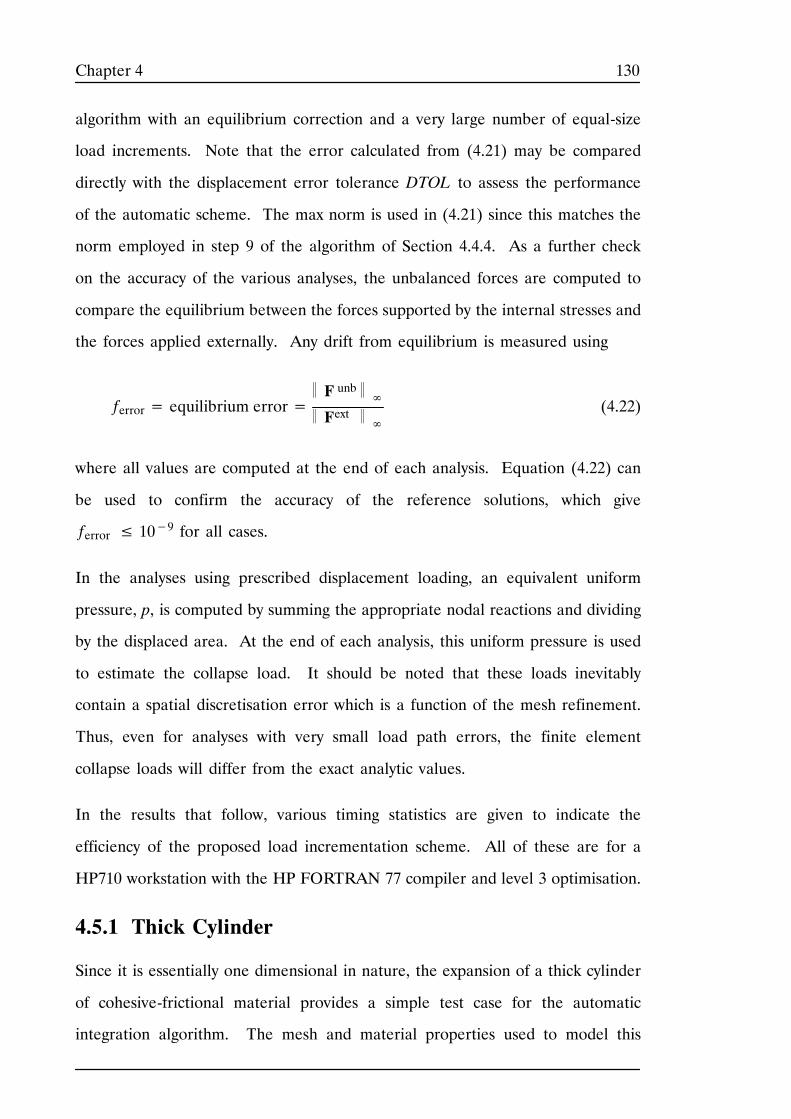
130Chapter 4
algorithm with an equilibrium correction and a very large number of equal-size
load increments. Note that the error calculated from (4.21) may be compared
directly with the displacement error tolerance DTOL to assess the performance
of the automatic scheme. The max norm is used in (4.21) since this matches the
norm employed in step 9 of the algorithm of Section 4.4.4. As a further check
on the accuracy of the various analyses, the unbalanced forces are computed to
compare the equilibrium between the forces supported by the internal stresses and
the forces applied externally. Any drift from equilibrium is measured using
ferror= equilibrium error= F unb ∞ Fext ∞
(4.22)
where all values are computed at the end of each analysis. Equation (4.22) can
be used to confirm the accuracy of the reference solutions, which give
ferror ≤ 10−9 for all cases.
In the analyses using prescribed displacement loading, an equivalent uniform
pressure, p, is computed by summing the appropriate nodal reactions and dividing
by the displaced area. At the end of each analysis, this uniform pressure is used
to estimate the collapse load. It should be noted that these loads inevitably
contain a spatial discretisation error which is a function of the mesh refinement.
Thus, even for analyses with very small load path errors, the finite element
collapse loads will differ from the exact analytic values.
In the results that follow, various timing statistics are given to indicate the
efficiency of the proposed load incrementation scheme. All of these are for a
HP710 workstation with the HP FORTRAN 77 compiler and level 3 optimisation.
4.5.1 Thick Cylinder
Since it is essentially one dimensional in nature, the expansion of a thick cylinder
of cohesive-frictional material provides a simple test case for the automatic
integration algorithm. The mesh and material properties used to model this
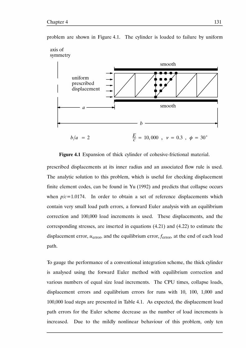
131Chapter 4
problem are shown in Figure 4.1. The cylinder is loaded to failure by uniform
b
Ec = 10, 000 , ν= 0.3 , φ= 30˚b∕a = 2
smooth
smooth
uniformprescribeddisplacement
axis ofsymmetry
a
Figure 4.1 Expansion of thick cylinder of cohesive-frictional material.
prescribed displacements at its inner radius and an associated flow rule is used.
The analytic solution to this problem, which is useful for checking displacement
finite element codes, can be found in Yu (1992) and predicts that collapse occurs
when p/c=1.0174. In order to obtain a set of reference displacements which
contain very small load path errors, a forward Euler analysis with an equilibrium
correction and 100,000 load increments is used. These displacements, and the
corresponding stresses, are inserted in equations (4.21) and (4.22) to estimate the
displacement error, uerror, and the equilibrium error, ferror, at the end of each load
path.
To gauge the performance of a conventional integration scheme, the thick cylinder
is analysed using the forward Euler method with equilibrium correction and
various numbers of equal size load increments. The CPU times, collapse loads,
displacement errors and equilibrium errors for runs with 10, 100, 1,000 and
100,000 load steps are presented in Table 4.1. As expected, the displacement load
path errors for the Euler scheme decrease as the number of load increments is
increased. Due to the mildly nonlinear behaviour of this problem, only ten
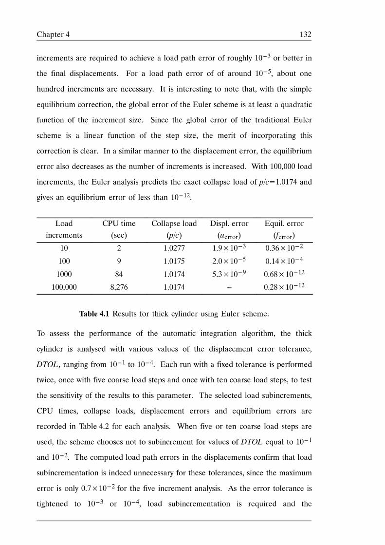
132Chapter 4
increments are required to achieve a load path error of roughly 10---3 or better in
the final displacements. For a load path error of of around 10---5, about one
hundred increments are necessary. It is interesting to note that, with the simple
equilibrium correction, the global error of the Euler scheme is at least a quadratic
function of the increment size. Since the global error of the traditional Euler
scheme is a linear function of the step size, the merit of incorporating this
correction is clear. In a similar manner to the displacement error, the equilibrium
error also decreases as the number of increments is increased. With 100,000 load
increments, the Euler analysis predicts the exact collapse load of p/c=1.0174 and
gives an equilibrium error of less than 10---12.
Loadincrements
CPU time(sec)
Collapse load(p/c)
Displ. error(uerror)
Equil. error(ferror)
10 2 1.0277 1.9×10---3 0.36×10---2
100 9 1.0175 2.0×10---5 0.14×10---4
1000 84 1.0174 5.3×10---9 0.68×10---12
100,000 8,276 1.0174 --- 0.28×10---12
Table 4.1 Results for thick cylinder using Euler scheme.
To assess the performance of the automatic integration algorithm, the thick
cylinder is analysed with various values of the displacement error tolerance,
DTOL, ranging from 10---1 to 10---4. Each run with a fixed tolerance is performed
twice, once with five coarse load steps and once with ten coarse load steps, to test
the sensitivity of the results to this parameter. The selected load subincrements,
CPU times, collapse loads, displacement errors and equilibrium errors are
recorded in Table 4.2 for each analysis. When five or ten coarse load steps are
used, the scheme chooses not to subincrement for values of DTOL equal to 10---1
and 10---2. The computed load path errors in the displacements confirm that load
subincrementation is indeed unnecessary for these tolerances, since the maximum
error is only 0.7×10---2 for the five increment analysis. As the error tolerance is
tightened to 10---3 or 10---4, load subincrementation is required and the
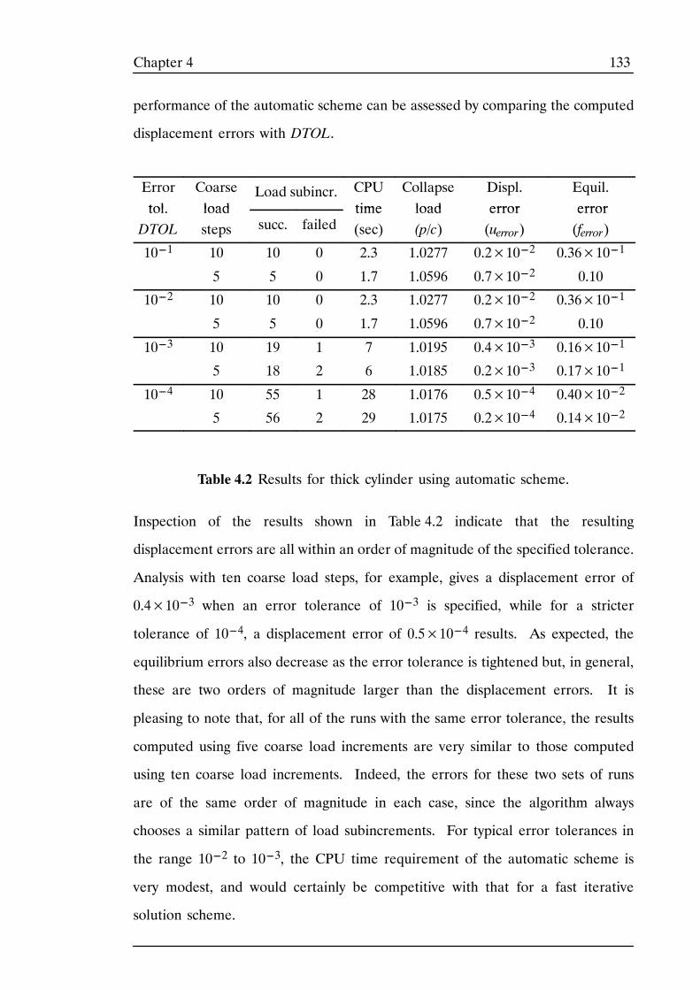
133Chapter 4
performance of the automatic scheme can be assessed by comparing the computed
displacement errors with DTOL.
Errortol
Coarseload
Load subincr. CPUtime
Collapseload
Displ.error
Equil.errortol.
DTOLloadsteps succ. failed
time(sec)
load(p/c)
error(uerror)
error(ferror)
10---1 10 10 0 2.3 1.0277 0.2×10---2 0.36×10---1
5 5 0 1.7 1.0596 0.7×10---2 0.10
10---2 10 10 0 2.3 1.0277 0.2×10---2 0.36×10---1
5 5 0 1.7 1.0596 0.7×10---2 0.10
10---3 10 19 1 7 1.0195 0.4×10---3 0.16×10---1
5 18 2 6 1.0185 0.2×10---3 0.17×10---1
10---4 10 55 1 28 1.0176 0.5×10---4 0.40×10---2
5 56 2 29 1.0175 0.2×10---4 0.14×10---2
Table 4.2 Results for thick cylinder using automatic scheme.
Inspection of the results shown in Table 4.2 indicate that the resulting
displacement errors are all within an order of magnitude of the specified tolerance.
Analysis with ten coarse load steps, for example, gives a displacement error of
0.4×10---3 when an error tolerance of 10---3 is specified, while for a stricter
tolerance of 10---4, a displacement error of 0.5×10---4 results. As expected, the
equilibrium errors also decrease as the error tolerance is tightened but, in general,
these are two orders of magnitude larger than the displacement errors. It is
pleasing to note that, for all of the runs with the same error tolerance, the results
computed using five coarse load increments are very similar to those computed
using ten coarse load increments. Indeed, the errors for these two sets of runs
are of the same order of magnitude in each case, since the algorithm always
chooses a similar pattern of load subincrements. For typical error tolerances in
the range 10---2 to 10---3, the CPU time requirement of the automatic scheme is
very modest, and would certainly be competitive with that for a fast iterative
solution scheme.
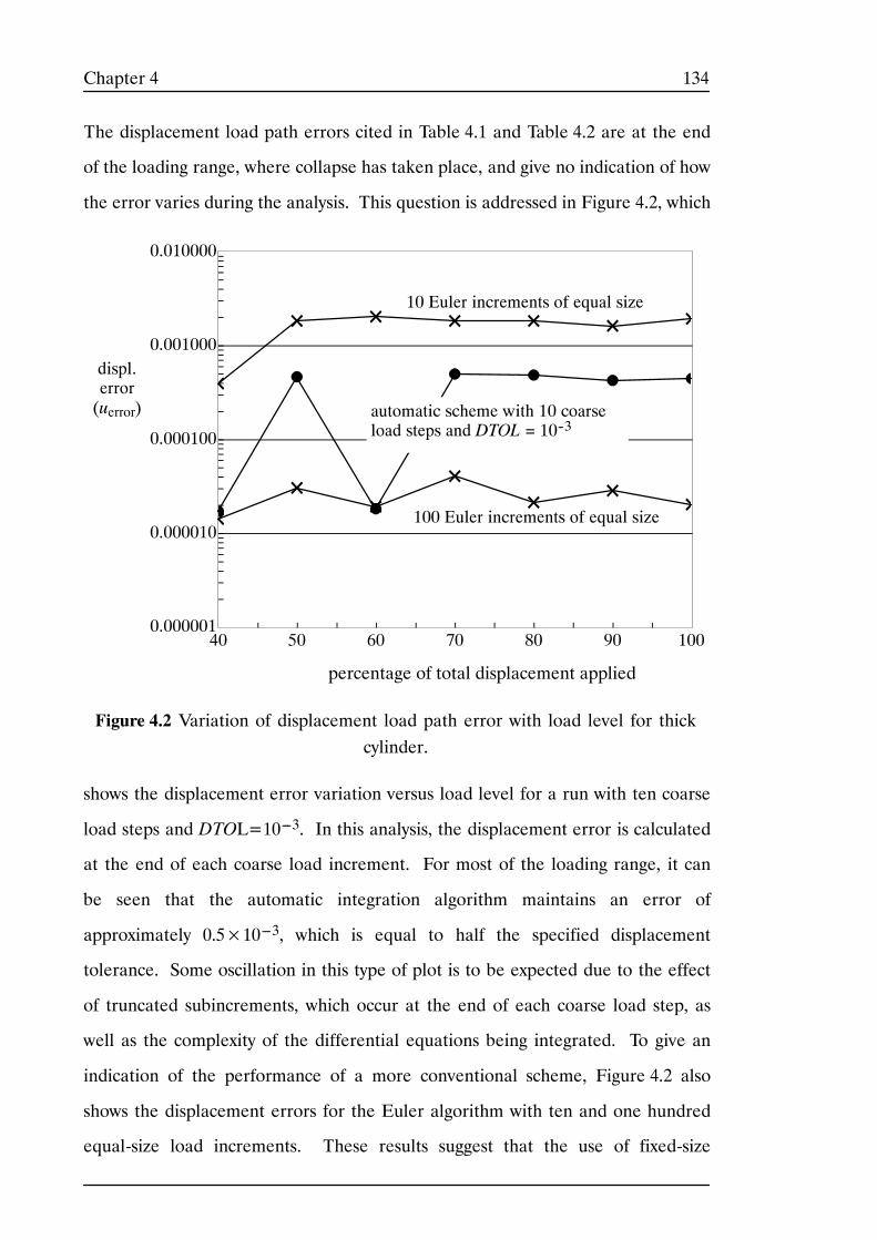
134Chapter 4
The displacement load path errors cited in Table 4.1 and Table 4.2 are at the end
of the loading range, where collapse has taken place, and give no indication of how
the error varies during the analysis. This question is addressed in Figure 4.2, which
0.000001
0.000010
0.000100
0.001000
0.010000
40 50 60 70 80 90 100
automatic scheme with 10 coarseload steps and DTOL = 10--3
percentage of total displacement applied
10 Euler increments of equal size
100 Euler increments of equal size
displ.error(uerror)
Figure 4.2 Variation of displacement load path error with load level for thickcylinder.
shows the displacement error variation versus load level for a run with ten coarse
load steps and DTOL=10---3. In this analysis, the displacement error is calculated
at the end of each coarse load increment. For most of the loading range, it can
be seen that the automatic integration algorithm maintains an error of
approximately 0.5×10---3, which is equal to half the specified displacement
tolerance. Some oscillation in this type of plot is to be expected due to the effect
of truncated subincrements, which occur at the end of each coarse load step, as
well as the complexity of the differential equations being integrated. To give an
indication of the performance of a more conventional scheme, Figure 4.2 also
shows the displacement errors for the Euler algorithm with ten and one hundred
equal-size load increments. These results suggest that the use of fixed-size
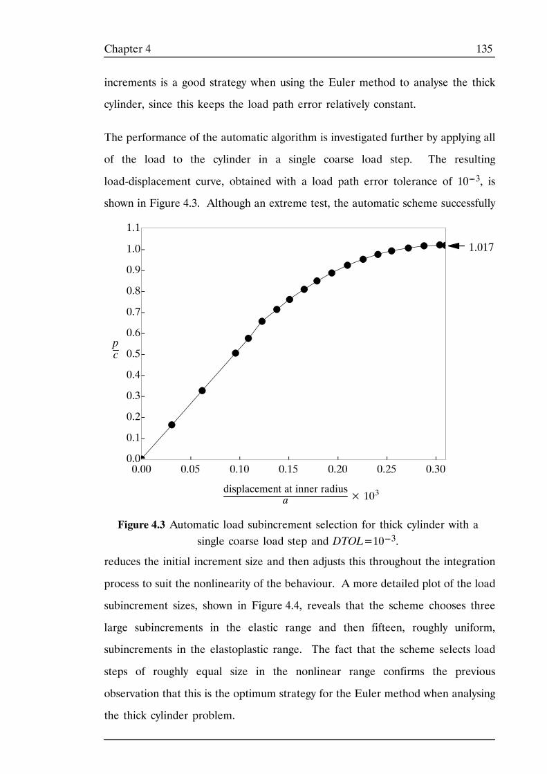
135Chapter 4
increments is a good strategy when using the Euler method to analyse the thick
cylinder, since this keeps the load path error relatively constant.
The performance of the automatic algorithm is investigated further by applying all
of the load to the cylinder in a single coarse load step. The resulting
load-displacement curve, obtained with a load path error tolerance of 10---3, is
shown in Figure 4.3. Although an extreme test, the automatic scheme successfully
0.0
0.1
0.2
0.3
0.4
0.5
0.6
0.7
0.8
0.9
1.0
1.1
0.00 0.05 0.10 0.15 0.20 0.25 0.30
pc
1.017
displacement at inner radiusa × 103
Figure 4.3 Automatic load subincrement selection for thick cylinder with asingle coarse load step and DTOL=10---3.
reduces the initial increment size and then adjusts this throughout the integration
process to suit the nonlinearity of the behaviour. A more detailed plot of the load
subincrement sizes, shown in Figure 4.4, reveals that the scheme chooses three
large subincrements in the elastic range and then fifteen, roughly uniform,
subincrements in the elastoplastic range. The fact that the scheme selects load
steps of roughly equal size in the nonlinear range confirms the previous
observation that this is the optimum strategy for the Euler method when analysing
the thick cylinder problem.
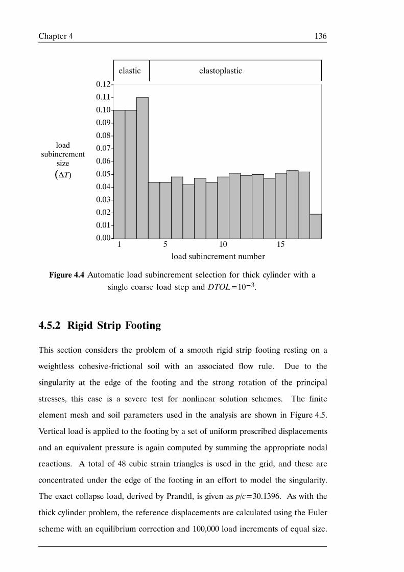
136Chapter 4
0.00
0.01
0.02
0.03
0.04
0.05
0.06
0.07
0.08
0.09
0.10
0.11
0.12
1 5 10 15
load subincrement number
elastoplasticelastic
(ΔT)
loadsubincrement
size
Figure 4.4 Automatic load subincrement selection for thick cylinder with asingle coarse load step and DTOL=10---3.
4.5.2 Rigid Strip Footing
This section considers the problem of a smooth rigid strip footing resting on a
weightless cohesive-frictional soil with an associated flow rule. Due to the
singularity at the edge of the footing and the strong rotation of the principal
stresses, this case is a severe test for nonlinear solution schemes. The finite
element mesh and soil parameters used in the analysis are shown in Figure 4.5.
Vertical load is applied to the footing by a set of uniform prescribed displacements
and an equivalent pressure is again computed by summing the appropriate nodal
reactions. A total of 48 cubic strain triangles is used in the grid, and these are
concentrated under the edge of the footing in an effort to model the singularity.
The exact collapse load, derived by Prandtl, is given as p/c=30.1396. As with the
thick cylinder problem, the reference displacements are calculated using the Euler
scheme with an equilibrium correction and 100,000 load increments of equal size.
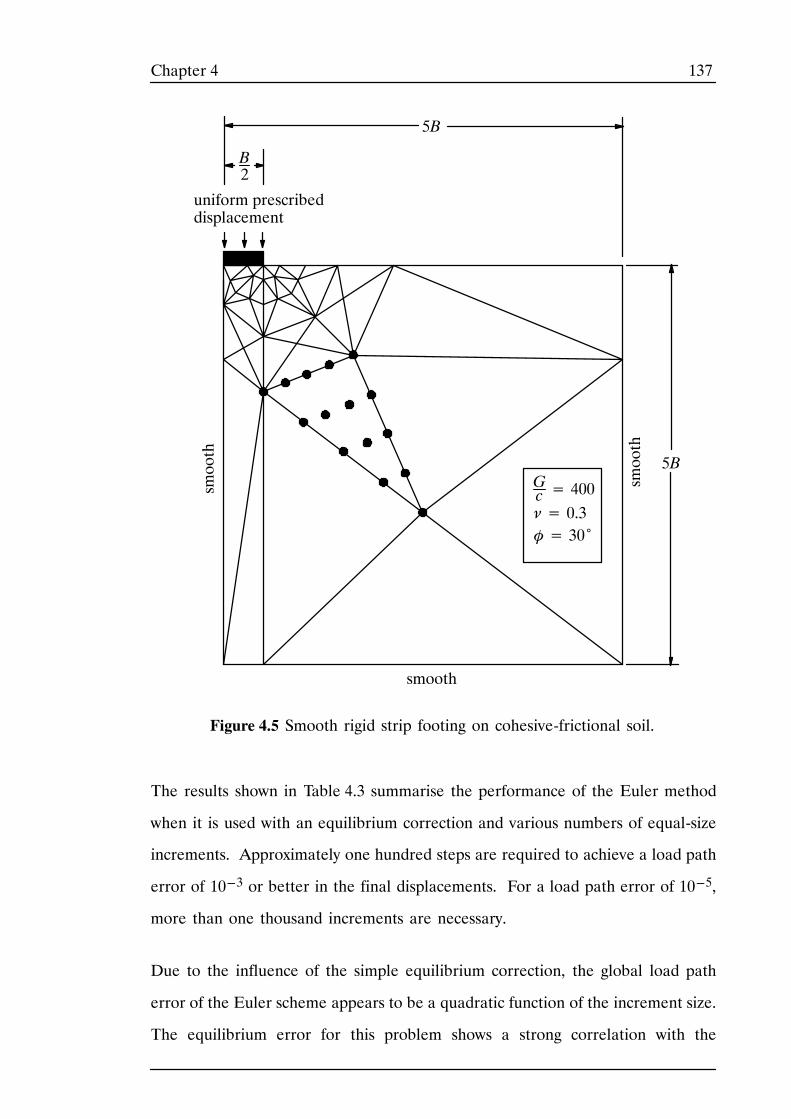
137Chapter 4
5B
B2
smooth
smooth
smooth
uniform prescribeddisplacement
5B
Figure 4.5 Smooth rigid strip footing on cohesive-frictional soil.
Gc = 400ν= 0.3φ= 30˚
The results shown in Table 4.3 summarise the performance of the Euler method
when it is used with an equilibrium correction and various numbers of equal-size
increments. Approximately one hundred steps are required to achieve a load path
error of 10---3 or better in the final displacements. For a load path error of 10---5,
more than one thousand increments are necessary.
Due to the influence of the simple equilibrium correction, the global load path
error of the Euler scheme appears to be a quadratic function of the increment size.
The equilibrium error for this problem shows a strong correlation with the
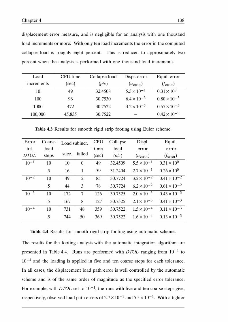
138Chapter 4
displacement error measure, and is negligible for an analysis with one thousand
load increments or more. With only ten load increments the error in the computed
collapse load is roughly eight percent. This is reduced to approximately two
percent when the analysis is performed with one thousand load increments.
Loadincrements
CPU time(sec)
Collapse load(p/c)
Displ. error(uerror)
Equil. error(ferror)
10 49 32.4508 5.5×10---1 0.31×100---
100 96 30.7530 6.4×10---3 0.80×10---3
1000 472 30.7522 3.2×10---5 0.57×10---5
100,000 45,835 30.7522 --- 0.42×10---9
Table 4.3 Results for smooth rigid strip footing using Euler scheme.
Errortol
Coarseload
Load subincr. CPUtime
Collapseload
Displ.error
Equil.errortol.
DTOLloadsteps succ. failed
time(sec)
load(p/c)
error(uerror)
error(ferror)
10---1 10 10 0 49 32.4509 5.5×10---1 0.31×100---
5 16 1 59 31.2404 2.7×10---1 0.26×100---
10---2 10 49 2 85 30.7724 3.2×10---2 0.41×10---2
5 44 3 78 30.7724 6.2×10---2 0.61×10---2
10---3 10 172 7 126 30.7525 2.0×10---3 0.43×10---3
5 167 8 127 30.7525 2.1×10---3 0.41×10---3
10---4 10 731 48 359 30.7522 1.5×10---4 0.11×10---3
5 744 50 369 30.7522 1.6×10---4 0.13×10---3
Table 4.4 Results for smooth rigid strip footing using automatic scheme.
The results for the footing analysis with the automatic integration algorithm are
presented in Table 4.4. Runs are performed with DTOL ranging from 10---1 to
10---4 and the loading is applied in five and ten coarse steps for each tolerance.
In all cases, the displacement load path error is well controlled by the automatic
scheme and is of the same order of magnitude as the specified error tolerance.
For example, with DTOL set to 10---1, the runs with five and ten coarse steps give,
respectively, observed load path errors of 2.7×10---1 and 5.5×10---1. With a tighter
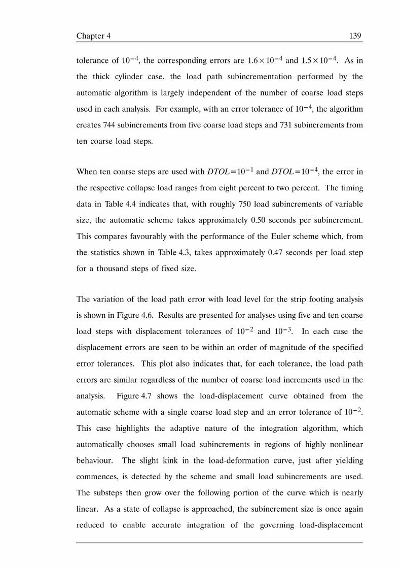
139Chapter 4
tolerance of 10---4, the corresponding errors are 1.6×10---4 and 1.5×10---4. As in
the thick cylinder case, the load path subincrementation performed by the
automatic algorithm is largely independent of the number of coarse load steps
used in each analysis. For example, with an error tolerance of 10---4, the algorithm
creates 744 subincrements from five coarse load steps and 731 subincrements from
ten coarse load steps.
When ten coarse steps are used with DTOL=10---1 and DTOL=10---4, the error in
the respective collapse load ranges from eight percent to two percent. The timing
data in Table 4.4 indicates that, with roughly 750 load subincrements of variable
size, the automatic scheme takes approximately 0.50 seconds per subincrement.
This compares favourably with the performance of the Euler scheme which, from
the statistics shown in Table 4.3, takes approximately 0.47 seconds per load step
for a thousand steps of fixed size.
The variation of the load path error with load level for the strip footing analysis
is shown in Figure 4.6. Results are presented for analyses using five and ten coarse
load steps with displacement tolerances of 10---2 and 10---3. In each case the
displacement errors are seen to be within an order of magnitude of the specified
error tolerances. This plot also indicates that, for each tolerance, the load path
errors are similar regardless of the number of coarse load increments used in the
analysis. Figure 4.7 shows the load-displacement curve obtained from the
automatic scheme with a single coarse load step and an error tolerance of 10---2.
This case highlights the adaptive nature of the integration algorithm, which
automatically chooses small load subincrements in regions of highly nonlinear
behaviour. The slight kink in the load-deformation curve, just after yielding
commences, is detected by the scheme and small load subincrements are used.
The substeps then grow over the following portion of the curve which is nearly
linear. As a state of collapse is approached, the subincrement size is once again
reduced to enable accurate integration of the governing load-displacement
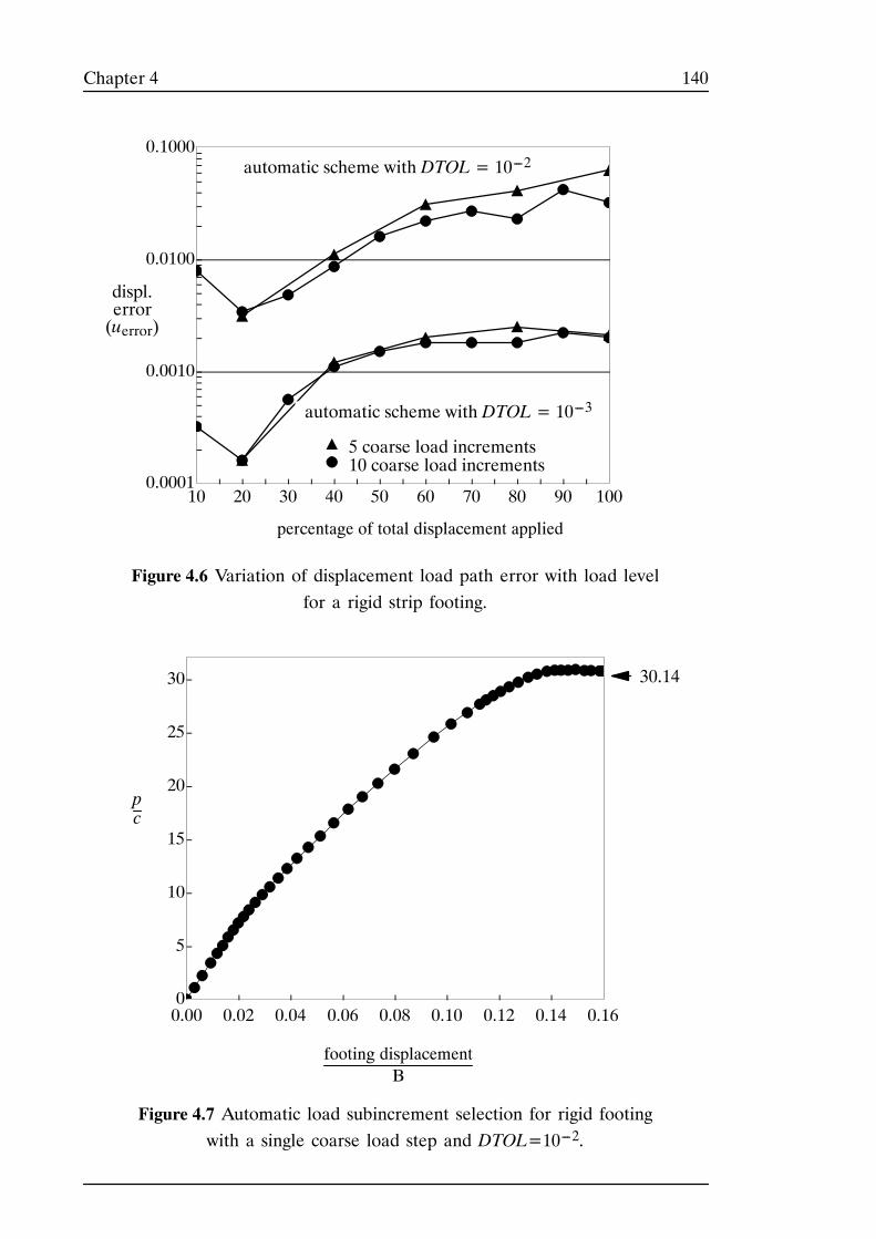
140Chapter 4
0.0001
0.0010
0.0100
0.1000
10 20 30 40 50 60 70 80 90 100
automatic scheme with DTOL = 10---3
displ.error(uerror)
percentage of total displacement applied
automatic scheme with DTOL = 10---2
5 coarse load increments10 coarse load increments
Figure 4.6 Variation of displacement load path error with load levelfor a rigid strip footing.
0
5
10
15
20
25
30
0.00 0.02 0.04 0.06 0.08 0.10 0.12 0.14 0.16
30.14
pc
footing displacementB
Figure 4.7 Automatic load subincrement selection for rigid footingwith a single coarse load step and DTOL=10---2.
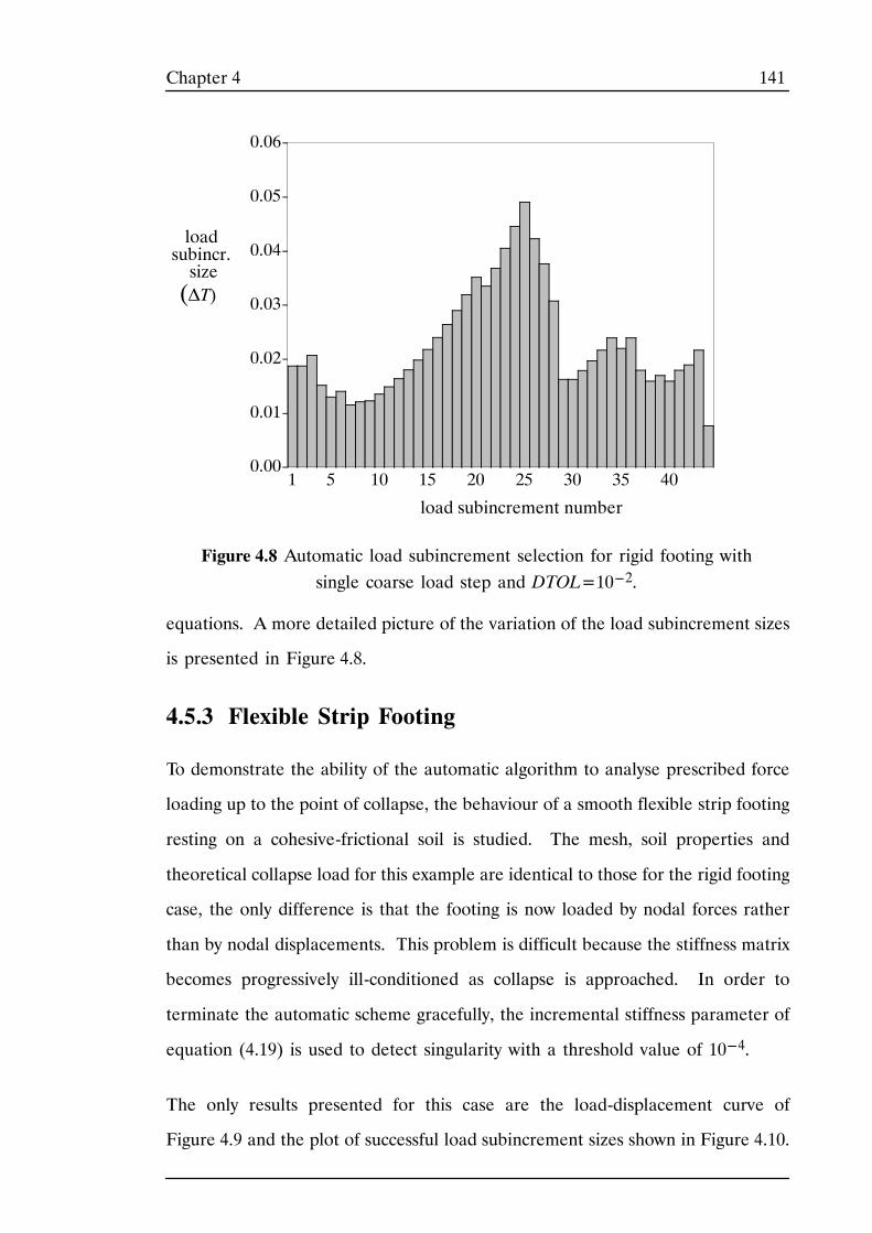
141Chapter 4
0.00
0.01
0.02
0.03
0.04
0.05
0.06
1 5 10 15 20 25 30 35 40
loadsubincr.size
load subincrement number
(ΔT)
Figure 4.8 Automatic load subincrement selection for rigid footing withsingle coarse load step and DTOL=10---2.
equations. A more detailed picture of the variation of the load subincrement sizes
is presented in Figure 4.8.
4.5.3 Flexible Strip Footing
To demonstrate the ability of the automatic algorithm to analyse prescribed force
loading up to the point of collapse, the behaviour of a smooth flexible strip footing
resting on a cohesive-frictional soil is studied. The mesh, soil properties and
theoretical collapse load for this example are identical to those for the rigid footing
case, the only difference is that the footing is now loaded by nodal forces rather
than by nodal displacements. This problem is difficult because the stiffness matrix
becomes progressively ill-conditioned as collapse is approached. In order to
terminate the automatic scheme gracefully, the incremental stiffness parameter of
equation (4.19) is used to detect singularity with a threshold value of 10---4.
The only results presented for this case are the load-displacement curve of
Figure 4.9 and the plot of successful load subincrement sizes shown in Figure 4.10.
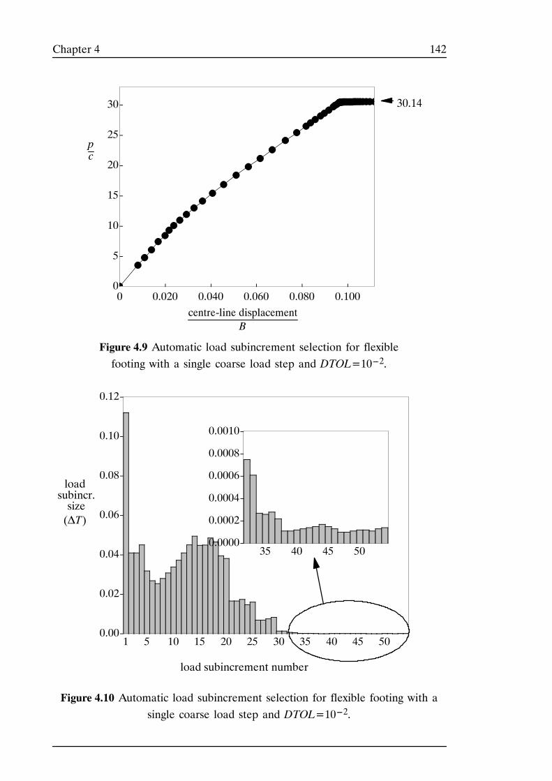
142Chapter 4
30.14
pc
0
5
10
15
20
25
30
0 0.020 0.040 0.060 0.080 0.100
centre-line displacementB
Figure 4.9 Automatic load subincrement selection for flexiblefooting with a single coarse load step and DTOL=10---2.
loadsubincr.size
load subincrement number
(ΔT)
0.00
0.02
0.04
0.06
0.08
0.10
0.12
1 5 10 15 20 25 30 35 40 45 50
0.0000
0.0002
0.0004
0.0006
0.0008
0.0010
35 40 45 50
Figure 4.10 Automatic load subincrement selection for flexible footing with asingle coarse load step and DTOL=10---2.
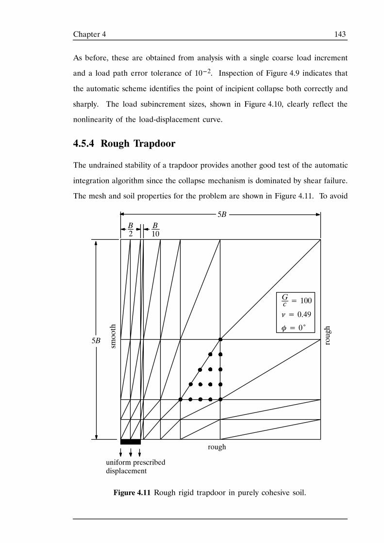
143Chapter 4
As before, these are obtained from analysis with a single coarse load increment
and a load path error tolerance of 10---2. Inspection of Figure 4.9 indicates that
the automatic scheme identifies the point of incipient collapse both correctly and
sharply. The load subincrement sizes, shown in Figure 4.10, clearly reflect the
nonlinearity of the load-displacement curve.
4.5.4 Rough Trapdoor
The undrained stability of a trapdoor provides another good test of the automatic
integration algorithm since the collapse mechanism is dominated by shear failure.
The mesh and soil properties for the problem are shown in Figure 4.11. To avoid
B2
B10
rough
rough
uniform prescribeddisplacement
5B
5B
smooth
Figure 4.11 Rough rigid trapdoor in purely cohesive soil.
Gc = 100
ν= 0.49
φ= 0˚
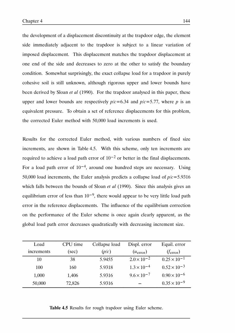
144Chapter 4
the development of a displacement discontinuity at the trapdoor edge, the element
side immediately adjacent to the trapdoor is subject to a linear variation of
imposed displacement. This displacement matches the trapdoor displacement at
one end of the side and decreases to zero at the other to satisfy the boundary
condition. Somewhat surprisingly, the exact collapse load for a trapdoor in purely
cohesive soil is still unknown, although rigorous upper and lower bounds have
been derived by Sloan et al (1990). For the trapdoor analysed in this paper, these
upper and lower bounds are respectively p/c=6.34 and p/c=5.77, where p is an
equivalent pressure. To obtain a set of reference displacements for this problem,
the corrected Euler method with 50,000 load increments is used.
Results for the corrected Euler method, with various numbers of fixed size
increments, are shown in Table 4.5. With this scheme, only ten increments are
required to achieve a load path error of 10---2 or better in the final displacements.
For a load path error of 10---4, around one hundred steps are necessary. Using
50,000 load increments, the Euler analysis predicts a collapse load of p/c=5.9316
which falls between the bounds of Sloan et al (1990). Since this analysis gives an
equilibrium error of less than 10---9, there would appear to be very little load path
error in the reference displacements. The influence of the equilibrium correction
on the performance of the Euler scheme is once again clearly apparent, as the
global load path error decreases quadratically with decreasing increment size.
Loadincrements
CPU time(sec)
Collapse load(p/c)
Displ. error(uerror)
Equil. error(ferror)
10 38 5.9455 2.0×10---2 0.25×10---1
100 160 5.9318 1.3×10---4 0.52×10---3
1,000 1,406 5.9316 9.6×10---7 0.90×10---6
50,000 72,826 5.9316 --- 0.35×10---9
Table 4.5 Results for rough trapdoor using Euler scheme.
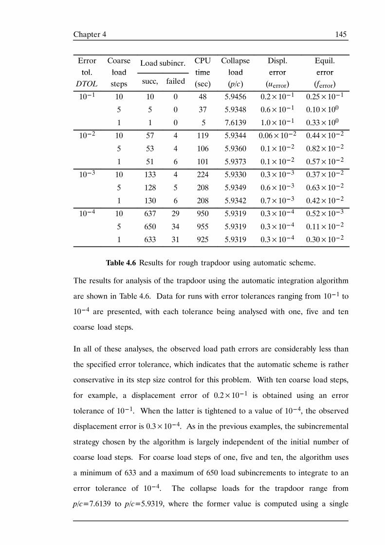
145Chapter 4
Errortol
Coarseload
Load subincr. CPUtime
Collapseload
Displ.error
Equil.errortol.
DTOLloadsteps succ, failed
time(sec)
load(p/c)
error(uerror)
error(ferror)
10---1 10 10 0 48 5.9456 0.2×10---1 0.25×10---1
5 5 0 37 5.9348 0.6×10---1 0.10×100---
1 1 0 5 7.6139 1.0×10---1 0.33×100---
10---2 10 57 4 119 5.9344 0.06×10---2 0.44×10---2
5 53 4 106 5.9360 0.1×10---2 0.82×10---2
1 51 6 101 5.9373 0.1×10---2 0.57×10---2
10---3 10 133 4 224 5.9330 0.3×10---3 0.37×10---2
5 128 5 208 5.9349 0.6×10---3 0.63×10---2
1 130 6 208 5.9342 0.7×10---3 0.42×10---2
10---4 10 637 29 950 5.9319 0.3×10---4 0.52×10---3
5 650 34 955 5.9319 0.3×10---4 0.11×10---2
1 633 31 925 5.9319 0.3×10---4 0.30×10---2
Table 4.6 Results for rough trapdoor using automatic scheme.
The results for analysis of the trapdoor using the automatic integration algorithm
are shown in Table 4.6. Data for runs with error tolerances ranging from 10---1 to
10---4 are presented, with each tolerance being analysed with one, five and ten
coarse load steps.
In all of these analyses, the observed load path errors are considerably less than
the specified error tolerance, which indicates that the automatic scheme is rather
conservative in its step size control for this problem. With ten coarse load steps,
for example, a displacement error of 0.2×10---1 is obtained using an error
tolerance of 10---1. When the latter is tightened to a value of 10---4, the observed
displacement error is 0.3×10---4. As in the previous examples, the subincremental
strategy chosen by the algorithm is largely independent of the initial number of
coarse load steps. For coarse load steps of one, five and ten, the algorithm uses
a minimum of 633 and a maximum of 650 load subincrements to integrate to an
error tolerance of 10---4. The collapse loads for the trapdoor range from
p/c=7.6139 to p/c=5.9319, where the former value is computed using a single
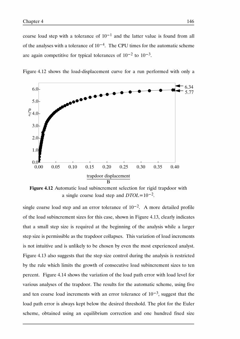
146Chapter 4
coarse load step with a tolerance of 10---1 and the latter value is found from all
of the analyses with a tolerance of 10---4. The CPU times for the automatic scheme
are again competitive for typical tolerances of 10---2 to 10---3.
Figure 4.12 shows the load-displacement curve for a run performed with only a
0.0
1.0
2.0
3.0
4.0
5.0
6.0
0.00 0.05 0.10 0.15 0.20 0.25 0.30 0.35 0.40
pc
6.345.77
trapdoor displacementB
Figure 4.12 Automatic load subincrement selection for rigid trapdoor witha single coarse load step and DTOL=10---2.
single coarse load step and an error tolerance of 10---2. A more detailed profile
of the load subincrement sizes for this case, shown in Figure 4.13, clearly indicates
that a small step size is required at the beginning of the analysis while a larger
step size is permissible as the trapdoor collapses. This variation of load increments
is not intuitive and is unlikely to be chosen by even the most experienced analyst.
Figure 4.13 also suggests that the step size control during the analysis is restricted
by the rule which limits the growth of consecutive load subincrement sizes to ten
percent. Figure 4.14 shows the variation of the load path error with load level for
various analyses of the trapdoor. The results for the automatic scheme, using five
and ten coarse load increments with an error tolerance of 10---3, suggest that the
load path error is always kept below the desired threshold. The plot for the Euler
scheme, obtained using an equilibrium correction and one hundred fixed size
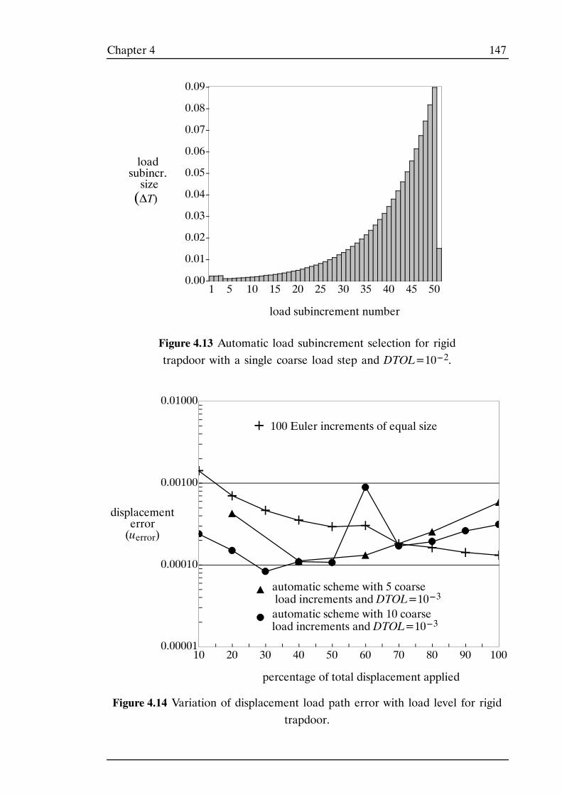
147Chapter 4
loadsubincr.size
load subincrement number
(ΔT)
0.00
0.01
0.02
0.03
0.04
0.05
0.06
0.07
0.08
0.09
1 5 10 15 20 25 30 35 40 45 50
Figure 4.13 Automatic load subincrement selection for rigidtrapdoor with a single coarse load step and DTOL=10---2.
0.00001
0.00010
0.00100
0.01000
10 20 30 40 50 60 70 80 90 100
displacementerror(uerror)
percentage of total displacement applied
100 Euler increments of equal size
automatic scheme with 5 coarseload increments and DTOL=10---3
automatic scheme with 10 coarseload increments and DTOL=10---3
Figure 4.14 Variation of displacement load path error with load level for rigidtrapdoor.
148Chapter 4
steps, indicates that the use of equal size increments leads to decreasing load path
error with increasing load level. This data supports the strategy of the automatic
scheme, which tries to keep the load path error constant by increasing the
subincrement size as the load is increased.
4.6 CONCLUSIONS
The explicit modified Euler algorithm is a robust and efficient method for
integrating the global stiffness equations in nonlinear finite element analysis. By
automatically subincrementing a number of user-defined coarse load steps, the
scheme is able to solve the governing relations so that the load path error in the
final displacements lies near a specified tolerance. The technique successfully
controls this error independently of the number of coarse load increments supplied
by the user, and may even be employed with a single coarse load step.
149Chapter 5
CHAPTER 5
INTEGRATION OF
CONSOLIDATION RELATIONS
150Chapter 5
5.1 INTRODUCTION
This Chapter describes a new finite element algorithm for solving elastic and
elastoplastic coupled consolidation problems. The procedure treats the governing
consolidation relations as a system of first order differential equations and is based
on the Backward Euler scheme with automatic subincrementation of a prescribed
series of time increments. The prescribed time increments, which are sometimes
called coarse time steps, serve to start the procedure and are chosen by the user.
In a similar manner to the load-stepping scheme described in Chapter 4, the
automatic consolidation algorithm attempts to choose the time subincrements such
that, for a given mesh, the time-stepping (or temporal discretisation) error in the
displacements lies close to specified tolerance.
Unlike existing solution techniques, the new algorithm computes not only the
displacements and pore pressures, but also their derivatives with respect to time.
These extra variables permit a family of unconditionally stable integration
algorithms to be constructed which automatically provide an estimate of the local
truncation error for each time step. This error estimate is very cheap to compute
and may be used to develop a simple and efficient automatic time stepping
mechanism. For the elastic case, the displacements and pore pressures at the end
of each subincrement may be solved directly without the need for iteration. For
elastoplastic behaviour, however, the governing relationships are nonlinear and a
system of nonlinear equations must be solved to compute the updates.
5.2 BACKGROUND
The finite element method can be used to model coupled consolidation using a
mixed formulation which incorporates displacement and pore pressure freedoms.
Even for elastic material behaviour, the resulting governing equations are
nonlinear due to the dissipation of excess pore water pressures. The solution of
these equations requires the linearisation of the time domain into a number a
discrete time increments, each of which is considered in sequence, and is difficult
151Chapter 5
to attempt by trial and error. The primary difficulty is due to the fact that an
acceptable increment size may vary by several orders of magnitude throughout the
analysis. During the early stages of consolidation, where excess pore water
pressure gradients are usually high, relatively small time increments are necessary
to obtain an accurate solution. As the analysis proceeds, however, much larger
time increments can be used with safety. Indeed, large increments are often
mandatory in order to obtain an efficient solution over a long period of
consolidation.
Terzaghi (1960) was the first to consider the analysis of consolidation and based
his formulation on the theory of diffusion. Nowadays, the numerical analysis of
consolidation is usually founded on the theory of Biot (1941), for which Sandu and
Wilson (1969) were the first to present a solution using finite elements. Since then
numerous researchers, including Christian and Boehemer (1970), Hwang et al
(1971), Yokoo, Yamagata and Nagaoka (1971a), Krause (1978), and Borja (1986)
have formulated the governing finite element equations for elastic materials. For
nonlinear materials, incremental solution strategies have been given by Lewis et
al (1976), Small et al (1976), Prevost (1982), and Borja (1989). Other solution
methods have been presented by Carter et al (1977 and 1979), who incorporated
the effects of finite deformations, while pore fluid compressibility was considered
by Gaboussi and Wilson (1973). In each of these formulations, whether linear or
nonlinear, the governing finite element relations can be expressed as a system of
coupled differential equations.
Techniques for the finite element solution of consolidation problems usually
involve a simple one dimensional time integration scheme, the stability and
accuracy of which has been investigated by Booker and Small (1975) and Vermeer
and Verruijt (1981). For elastic soils, the resulting time stepping schemes are
essentially the same as those used in the solution of first order systems of
differential equations. Since these types of equations arise in many areas of the
152Chapter 5
physical sciences, they have been studied extensively and a vast amount of
literature exists on their solution. An excellent summary of the stability and
accuracy of various algorithms can be found in Wood (1990). In order to solve
elastic coupled consolidation problems efficiently with the well known θ-method,
it is generally necessary to use an implicit time integration scheme with θ≥ 0.5.
With this choice of integration parameter, Booker and Small (1975) proved that
the solution process is unconditionally stable so that large time increments may
be used with safety. Explicit integration methods, which employ θ= 0, are only
conditionally stable and may require the use of very small time steps.
In the analysis of elastoplastic soils, the application of implicit time integration
schemes requires the solution of a system of nonlinear equations for each time
step. Small et al (1976) solved these nonlinear equations with an initial stiffness
iteration scheme which used averaged values of all time varying quantities. This
approach has been adopted by Siriwardane and Desai (1981), who also present an
alternative tangent stiffness update with no iteration.
Somewhat surprisingly, very little work has been done on the development of
automatic time stepping algorithms for finite element analysis of consolidation.
In a more general context, a number of schemes for controlling the increment size
during the solution of second order differential equations have been presented by
Zienkiewicz et al (1984) and Thomas and Gladwell (1988a). All of these methods
use an estimate of the local truncation error to regulate the step size and were
developed for the analysis of dynamic problems, such as those that occur in
earthquake loading. Although the schemes in Zienkiewicz et al (1984) use a Taylor
series expansion to estimate the local error, and permit the time increments to
expand or contract, they make no effort to control the error in the solution
directly. Thomas and Gladwell (1988a), on the other hand, take the difference
between solutions from p and p+1 stage schemes as an estimate of the local
truncation error and attempt to constrain this precisely by adaptive control of the
153Chapter 5
increment size. A key advantage of these methods is that they operate in single
step mode and, hence, do not need to use values generated in previous time
increments. Moreover, their local error estimators are embedded and can be
computed cheaply with no extra matrix factorisations. The two methods proposed
by Thomas and Gladwell (1988a) are aimed at systems of second order differential
equations and are based on a first order accurate 2---stage/second order accurate
3---stage pair and a second order accurate 3---stage/third order accurate 4---stage
pair. The latter is only conditionally stable but has a large region of stability. In
a companion paper, Gladwell and Thomas (1988b) discuss implementation issues
associated with their formulas and give an example code to illustrate the
computational detail.
The scheme presented in this Chapter differs from those of Thomas and Gladwell
(1988a) in that it uses a first order accurate 1-stage/second order accurate 2-stage
pair of integration schemes to estimate the local truncation error for systems of
first order differential equations. The proposed scheme enables the truncation
error to be estimated using a single factorisation and solution of the matrix
equations.
5.3 FORMULATION OF GOVERNING BIOTCONSOLIDATION EQUATIONS
Consider a porous body of volume V and surface area S whose pores are filled
with water. During the consolidation process, the distribution of the stresses
within the body is governed by the principles of effective stress, equilibrium, and
continuity of flow. These principles are all invoked to obtain the governing finite
element equations.
The effective stress principle assumes that the total stresses, σ, comprise the sum
of the effective stresses, σ′, and the pore water pressure, p, according to
σ= σ′ +m p (5.1)
154Chapter 5
where m= {1, 1, 1, 0, 0, 0}T and tensile stresses and pore pressures are taken as
positive. Differentiating this equation with respect to time gives
σ. = σ. ′ +m p. (5.2)
In geotechnical analysis, it is conventional to decompose the total pore pressure
into a steady state component, ps, and a time-varying excess component, pe,
according to
p= ps+ pe (5.3)
Noting that ps is constant, differentiation of (5.3) with respect to time gives
p. = p. e (5.4)
For applications which involve a horizontal phreatic surface, the steady state pore
pressure component corresponds to a hydrostatic stress distribution. To determine
the governing relations for finite element analysis of consolidation, the effective
stresses and pore pressures are treated separately and the primary nodal variables
are the displacement rates (velocities) and the pore pressure rates. Because of
the equivalence established in equation (5.4), there is little to choose between
working with total pore pressure rates or excess pore pressure rates. In this Thesis,
the formulation will be developed in terms of total pore pressure rates.
As described in Chapter 2, the method of weighted residuals can be used to
express the three dimensional equations of equilibrium in the weak form
V
(∇w)Tσ dV−V
wTbdV−S
wT tdS= 0 (5.5)
where ∇ denotes the differential operator defined by equation (2.15),
w= wx , wy , wzTis a vector of arbitrary weighting functions in the three
coordinate directions, σ= σx , σy , σz , τxy , τxz , τyzTare the total stresses within
the soil mass, b= bx , by , bzTare the applied body forces, and t= tx , ty , tz
Tis
a vector of external surface tractions acting over the boundary surface S.
155Chapter 5
Differentiating (5.5) with respect to time and substituting (5.2) furnishes the
equilibrium equations in rate form according to
V
(∇w)T (σ. ′ +mp. )dV−V
wTb.dV−
S
wT t.dS= 0 (5.6)
Following the procedure described in Chapter 2, a finite element solution to (5.6)
can be obtained by using shape functions to describe the variation of the velocities
and pore pressure rates throughout each element. For an element with n nodes,
the velocity field at any internal point is assumed to be of the form
d.= Nuu
.
where d.= u. , v. ,w. is a velocity vector with components u. , v. and w. in each
coordinate direction, Nu is a matrix of shape functions given by
Nu=⎪⎪⎡
⎣
Nu100
0Nu10
00Nu1
Nu200
0Nu20
00Nu2
...
...
...
Nun00
0Nun0
00Nun⎪⎪⎤
⎦
and u. = u. 1, v. 1, w. 1, u. 2, v. 2, w. 2, ... u. n, v. n , w. nTis a vector of element nodal
velocities.
Similarly, the field of pore pressure rates for an element with pore pressure
freedoms at m nodes is assumed to be of the form
p. = Npp. (5.7)
where
Np= Np1 Np2 ... Npm (5.8)
and
p. = p. 1, p.2, ... p
.mT
156Chapter 5
are, respectively, a matrix of shape functions and a vector of nodal pore pressure
rates. Note that, for generality, different sets of shape functions may be used to
describe the variation of the velocities and the pore pressure rates. This implies
that the nodes in the finite element mesh may have varying degrees of freedom,
with some being associated with velocities, some being associated with pore
pressure rates, and some being associated with both. In order for the pore
pressure rates to be consistent with the stress rates, it is usual to choose the
polynomial describing the pore pressure rates to be one order lower than the
polynomial describing the velocities. As discussed by a number of researchers,
including Yokoo, Yamagata and Nagaoka (1971a) and Sandhu, Lui and Singh
(1977), this approach leads to less accurate estimates of the settlements but much
smaller oscillations in the pore pressures.
Having defined the functional form of the velocities and pore pressure rates, the
Galerkin weighting functions may be chosen as
w= δd.= Nu δu
. (5.9)
where δu. is a vector of arbitrary nodal velocities for an element. Substituting
these weighting functions (5.9) into (5.6), integrating over the element volume, V e,
and surface area, Se, and collecting terms furnishes
δu. T⎪⎧⎩Ve
∇NuTσ. ′ dV+
Ve
∇NuTm p. dV−
SeNTu t
.dS−
VeNTu b
.dV⎪⎫⎭= 0
Since the velocities δu. are arbitrary, it follows that
VeBTuσ
. ′ dV+VeBTum p
. dV−SeNTu t
.dS−
VeNTu b
.dV= 0 (5.10)
where Bu is the strain rate-velocity matrix
157Chapter 5
Bu= ∇N=
⎪⎪⎪⎪⎪⎪⎪⎪⎪⎪⎪⎪⎪⎪⎪⎪
⎡
⎣
∂Nu1∂x
0
0
∂Nu1∂y∂Nu1∂z
0
0
∂Nu1∂y
0
∂Nu1∂x
0
∂Nu1∂z
0
0
∂Nu1∂z
0
∂Nu1∂x∂Nu1∂y
...
...
...
...
...
...
∂Nun∂x
0
0
∂Nun∂y∂Nun∂z
0
0
∂Nun∂y
0
∂Nun∂x
0
∂Nun∂z
0
0
∂Nun∂z
0
∂Nun∂x∂Nun∂y
⎪⎪⎪⎪⎪⎪⎪⎪⎪⎪⎪⎪⎪⎪⎪⎪
⎤
⎦
and the strain rates at any internal point are
ε. = ∇d
.= ∇Nu u
. = Buu. (5.11)
In the theory of elastoplasticity, the effective stress rates are assumed to be related
to the strain rates via the constitutive law
σ. ′ = Dep ε
.
where Dep is the elastoplastic constitutive matrix derived in Section 2.2.
Combining this equation with (5.11) permits the effective stresses to be expressed
in terms of the element nodal velocities according to
σ. ′ = Dep Buu
. (5.12)
Substituting (5.7) and (5.12) into (5.10) gives a weak statement of the conditions
of equilibrium for an element in rate form. These equations may be written as
kepu. + l p. = f
. ext (5.13)
where
kep= VeBTu Dep Bu dV (5.14)
l= VeBTu m Np dV (5.15)
158Chapter 5
are the elemental elastoplastic stiffness and coupling matrices and
f. ext=
VeNTu b
.dV+
SeNTu t
.dS (5.16)
is the elemental vector of external force rates.
In order to complete the mathematical description of the consolidation process,
it is necessary to consider the continuity of flow for an element of soil. Assuming
that the pore water and soil grains are incompressible, continuity of flow demands
that the rate at which water is drained from the soil skeleton must be equal to the
rate of volume decrease of the soil mass. This condition may be expressed
mathematically as
∂vx∂x +
∂vy∂y +
∂vz∂z =− (ε
.x+ ε
.y+ ε
.z )
or
div v+mT ε. = 0 (5.17)
where v= vx , vy , vzT denotes a vector of superficial (or bulk) fluid velocities and
ε. = ε. x , ε. y , ε. z , γ. xy , γ. xz , γ. yzT denotes a vector of strain rates for the soil. Thecontinuity equation may be expressed in terms of the pore water pressure using
Darcy’s law which, assuming a horizontal phreatic surface, states that the fluid
velocities are given by
vx=kxγw∂p∂x =
kxγw∂pe∂x
vy=kyγw∂p∂y− γw = kyγw ∂pe∂y
vz=kzγw∂p∂z =
kzγw∂pe∂z
where γw is the unit weight of water and kx, ky, kz are soil permeabilities in the
three coordinate directions. Note that, because compressive pore pressures are
159Chapter 5
taken as negative, the sign convention in the above equations is different to that
normally used in soil mechanics. Darcy’s law may also be written in the more
compact matrix form
v= kγw∇p− bw (5.18)
where bw= 0, γw , 0Tis a body force vector and k is a matrix of permeabilities
of the form
k=⎪⎡
⎣
kx00
0ky0
00kz⎪⎤
⎦
Inserting (5.18) into (5.17) gives the continuity equation in terms of the pore
pressures according to
div kγw ∇p− bw +mT ε. = div kγw ∇pe +mT ε. = 0
The weak form of this equation is obtained by applying the method of weighted
residuals with a Galerkin weight function, ω, according to
V
ωdiv kγw ∇p− bwdV+V
ωmT ε. dV= 0
Integrating the first term using the Green-Gauss theorem this becomes
S
ω ∇p− bwT kγw n dS−
V
(∇ω)T kγw∇p− bw dV+
V
ωmTε. dV= 0
or
V
(∇ω)T kγw ∇pdV−V
ωmTε. dV−S
ω qdS−V
(∇ω)T kγw bw dV= 0 (5.19)
where
160Chapter 5
q= ∇p− bwT kγwn= v
Tn
is a prescribed outward flow per unit area and n= nx , ny , nz Tis a vector of
direction cosines for the unit normal to S. To obtain the finite element counterpart
of (5.19), the pore pressure field for an element with m nodal pore pressures is
assumed to be of the form
p= Npp
where Np is given by (5.8) and
p= p1, p2, ... pmT
is a vector of nodal pore pressures. The Galerkin weight function is
ω= δp= Np δp (5.20)
where δp is an arbitrary set of nodal pore pressures for an element and
∇ω= ∇Np δp= Bp δp (5.21)
with
Bp = ∇Np=
⎪⎪⎪⎪⎪⎪⎪
⎡
⎣
∂Np1∂x∂Np1∂y∂Np1∂z
∂Np2∂x∂Np2∂y∂Np2∂z
...
...
...
∂Npm∂x∂Npm∂y∂Npm∂z
⎪⎪⎪⎪⎪⎪⎪
⎤
⎦
(5.22)
Substituting (5.11), (5.20), (5.21) and (5.22) in (5.19) and rearranging gives
δpT⎪⎧⎩VeNTp mTBudV u
. −VeBTp kγw Bp dV p−
SeNTp qdS−
VeBTp kγw bw dV⎪
⎫⎭= 0
where the integrations are now done over each element. As δpT is arbitrary, this
implies that
161Chapter 5
VeNTp mTBudV u
. −VeBTp kγw Bp dV p−
SeNTp qdS−
VeBTp kγw bw dV= 0
This equation expresses the continuity equation in weak form for each element
and may be written in the compact form
lTu. + hp= q (5.23)
where the coupling matrix l is given by (5.15), the flow matrix h is defined as
h=−VeBTp kγw Bp dV (5.24)
and
q= SeNTp qdS+
VeBTp kγw bw dV (5.25)
is a fluid supply vector. Equations (5.13) and (5.23), together with (5.14), (5.15),
(5.16), (5.24) and (5.25), define the governing relations for Biot consolidation at
the element level. Assembling the element matrices in the usual way produces
a global system of equations of the form
KepLTL
0U.P. +⎪⎡⎣
0
0
0
H⎪⎤⎦⎨⎧⎩U
P⎬⎫⎭= F
. ext
Q (5.26)
where
Kep= elements
kep= elements
VeBTu DepBudV
L= elements
l= elements
VeBTu mNp dV
H= elements
h=− elements
VeBTp kγw Bp dV
162Chapter 5
are the global elastoplastic stiffness, coupling and flow matrices and
F. ext=
elements
f. ext =
elements
VeNTu b
.dV+
elements
SeNTu t
.dS
Q= elements
q = elements
SeNTp qdS+
elements
VeBTp kγw bw dV
are the global external force rate and fluid supply vectors.
5.4 SOLUTION OF ELASTIC CONSOLIDATIONEQUATIONS
For the analysis of elastic solids with constant permeabilities, the relations (5.26)
constitute a system of linear first order differential equations of the form
CX.+ KX= F(t) (5.27)
where
C=⎪⎡⎣Ke
LT
L
0⎪⎤⎦
K=⎪⎡⎣0
0
0
H⎪⎤⎦
(5.28)
are matrices of constants, F(t) is a time dependent forcing function defined by
F(t)=⎨⎧⎩F. ext
Q⎬⎫⎭
(5.29)
and X= {U,P}T with X.= U. ,P. T. This type of system occurs in many areas of
engineering and science and has been widely studied. A very comprehensive
summary of the stability and accuracy of various solution strategies for solving
(5.27) may be found in Wood (1990). Since these methods are central to the work
undertaken in this Thesis, some of the more important techniques will now be
discussed.
163Chapter 5
5.4.1 Single-Step Schemes
The simplest strategy for solving (5.27) is commonly known as the θ-method. For
the nth time step ranging from tn−1 to tn= tn−1+ h, this algorithm may be
expressed in the form
[C+ θhK]Xn= C− (1− θ)hKXn−1+ h(1− θ) Fn+ θFn−1 (5.30)
where θ is an integration parameter in the interval 0≤ θ≤ 1, the subscripts n
and n− 1 denote, respectively, quantities evaluated at the start and end of the
step, and all values except Xn are known. The process assumes that X0 at time
t0 is known. For the case of an elastic soil with constant permeabilities, the
matrices C and K are independent of X and (5.30) defines a system of linear
equations which can be solved for Xn. Note that if h is kept constant, then the
matrix [C+ θhK] needs to be factorised only once to obtain the solution for all
time steps. Because θ may assume a range of values, equation (5.30) can be used
to generate a family of single-stage single-step schemes that all march the solution
X forward in time without the need for information from previous steps.
The θ-method is at least first order accurate and, provided θ≥ 0.5, is
unconditionally stable. Unconditionally stability is an essential characteristic for
an efficient consolidation scheme since it is often necessary to integrate over very
long time periods using large time steps. For the special case of θ= 0.5, the
θ-method is second order accurate and corresponds to the ubiquitous
Crank-Nicolson scheme. Although appealing because of its high accuracy, the
Crank-Nicolson method may generate spurious oscillations in the solution,
especially if there are abrupt changes in the forcing function, and often requires
special smoothing procedures such as those advocated by Wood and Lewis (1975)
and Wood (1977). Choosing a value of θ= 1 gives the well known backward
Euler scheme which is first order order accurate, unconditionally stable and
oscillation free (Wood, 1990). The last of these characteristics has led to the
164Chapter 5
Backward Euler method being widely used in finite element consolidation studies,
even though it is less accurate than the Crank-Nicolson scheme.
As an alternative to (5.30), the θ-method can be expressed in the more compact
form
[C+ θhK]V= (1− θ)Fn−1+ θFn−KXn−1 (5.31)
where
V= (Xn− Xn−1)∕h
is an average estimate of X.over the time step h and X is updated according to
Xn= Xn−1+ hV (5.32)
In the finite element literature, this form of the θ-method is often referred to as
the SS11 procedure, where the terminology SSpj stands for a Single-Step
algorithm which uses an approximation of degree p to solve a differential equation
of order j. These relations will be used to develop an automatic time stepping
scheme in later Sections of the Thesis.
5.4.2 Two-Step Schemes
A family of unconditionally stable second order accurate methods for solving
(5.27) can be derived by considering quantities generated over two consecutive
time steps. As discussed in Wood (1990), these schemes are of the general form
θ1hC+ 12 θ2h 2KXn= (1− θ1)hC+ 12 (2θ1− θ2− 1)h2KXn−2
+ (2θ1− 1)hC+ 12 (2θ2− 2θ1− 1)h2KXn−1
+12 (θ2− 2θ1+ 1) Fn−2+ 12 (2θ1− 2θ2+ 1) Fn−1+ 12 θ2Fn (5.33)
where θ1 and θ2 are specified, the subscripts n− 2 denote quantities evaluated
at tn−2= tn−1− h, and all values except Xn are assumed known. In order to
165Chapter 5
obtain unconditional stability, the integration parameters must be chosen such that
θ2> θ1≥ 0.5. For the special case of θ1− θ2= 0.5 and θ1> 0.5, the two-step
scheme is third order accurate but only conditionally stable. When C and K are
independent of X, equation (5.33) defines a system of linear equations which can
be solved to obtain Xn, the solution at the end of the current time step. As in
the case of the single-step schemes discussed previously, the two-step method
requires only one matrix factorisation if h is held constant throughout the solution
process.
One possible choice for the integration parameters is θ1= 0.5 and θ2= 2∕3.
These values, first suggested by Lees (1966), result in an algorithm that does not
require iteration for certain types of nonlinear problems, and have been used by
Lewis and Schrefler (1987) to model consolidation. According to the analysis
presented in Wood (1990), however, this method is subject to troublesome
oscillations and is not recommended.
Another possible alternative is the so-called backward difference scheme, which
is obtained by setting θ1= 1.5 and θ2= 2. Because of its ability to damp out
spurious high frequency components, this method is advocated by Richtmyer and
Morton (1967) and has also been used by Wood and Lewis (1975). In a detailed
study of various noise control strategies for the heat conduction equation, the
latter Authors conclude that, although the backward difference method does
indeed perform satisfactorily, an averaged form of the Crank-Nicolson scheme is
better still.
Other options that have been proposed for the integration parameters in (5.33)
include those of Liniger (1969), who suggests setting θ1= 1.218 and θ2= 1.292,
and Zlamal (1977), who recommends values of θ1= 5∕6 and θ2= 8∕9.
Unfortunately, no data is available to compare the performance of these schemes
in solving consolidation problems.
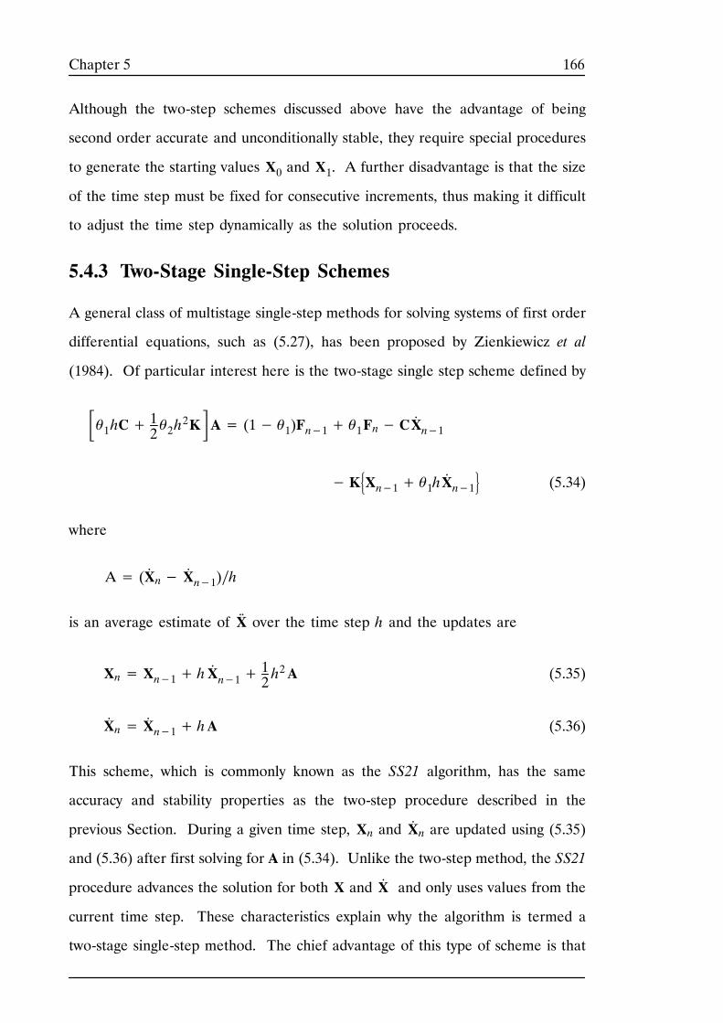
166Chapter 5
Although the two-step schemes discussed above have the advantage of being
second order accurate and unconditionally stable, they require special procedures
to generate the starting values X0 and X1. A further disadvantage is that the size
of the time step must be fixed for consecutive increments, thus making it difficult
to adjust the time step dynamically as the solution proceeds.
5.4.3 Two-Stage Single-Step Schemes
A general class of multistage single-step methods for solving systems of first order
differential equations, such as (5.27), has been proposed by Zienkiewicz et al
(1984). Of particular interest here is the two-stage single step scheme defined by
θ1hC+ 12 θ2h2KA= (1− θ1)Fn−1+ θ1Fn− CX.
n−1
−KXn−1+ θ1hX.
n−1 (5.34)
where
A= (X.n− X
.
n−1)∕h
is an average estimate of X..over the time step h and the updates are
Xn= Xn−1+ hX.
n−1+12 h2A (5.35)
X.n= X
.
n−1+ hA (5.36)
This scheme, which is commonly known as the SS21 algorithm, has the same
accuracy and stability properties as the two-step procedure described in the
previous Section. During a given time step, Xn and X.n are updated using (5.35)
and (5.36) after first solving for A in (5.34). Unlike the two-step method, the SS21
procedure advances the solution for both X and X.and only uses values from the
current time step. These characteristics explain why the algorithm is termed a
two-stage single-step method. The chief advantage of this type of scheme is that

167Chapter 5
the step size may be adjusted easily as the integration proceeds. The price of this
flexibility is the need to compute and store X.for each time step.
More recently, Thomas and Gladwell (1988a) have proposed a generalised form
of the SS21 algorithm. Their procedure uses three integration parameters instead
of two and may be written as
φ2hC+ φ3h2KA= Ft n−1+ φ1h − CX.
n−1−KXn−1+ φ1hX.
n−1 (5.37)
where A has the same meaning as before and the updates are again given by (5.35)
and (5.36). This scheme is second order accurate and unconditionally stable
provided 2φ3> φ1≥ 0.5 and φ2≥ 0.5. Using the fact that
Ft n−1+ φ1h = (1− φ1)Fn−1+ φ1Fn+O(h2) (5.38)
a comparison of equations (5.34) with (5.37) reveals that the SS21 algorithm of
Zienkiewicz et al (1984) is a special case of the Thomas and Gladwell algorithm
with θ1= φ1= φ2 and θ2= 2φ3. For cases where θ1= φ1= 1, this equivalence
holds without the need to approximate the forcing function by (5.38). Because of
the additional freedom that is introduced by having three integration parameters,
the Thomas and Gladwell method is ideally suited to the design of automatic
integration schemes with embedded error estimators. Indeed, it will be used for
this purpose in the next Section.
5.5 AUTOMATIC TIME STEPPING SCHEME FORELASTIC CONSOLIDATION
This Section describes an adaptive integration scheme that automatically adjusts
the time step according to a specified error criterion. For ease of use, the
algorithm assumes that a number of (coarse) time increments are defined and
automatically breaks these up into a number of smaller subincrements if necessary.
The coarse time step is assumed to start at t0 and end at t0 + Δt, and is thus of
size Δt. The nth time subincrement is assumed to be of size h, and ranges from
tn−1 to tn= tn−1+ h. This arrangement is shown schematically in Figure 5.1
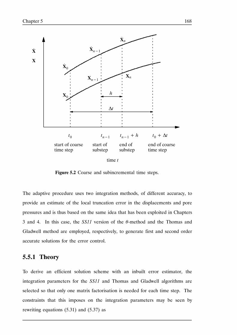
168Chapter 5
t0 t0+ Δttn−1 tn−1+ h
Xn−1
X.
n−1
X.n
Xn
h
X.
X
X0
X.
0
time t
start of coarsetime step
end of coarsetime step
Figure 5.2 Coarse and subincremental time steps.
Δt
start ofsubstep
end ofsubstep
The adaptive procedure uses two integration methods, of different accuracy, to
provide an estimate of the local truncation error in the displacements and pore
pressures and is thus based on the same idea that has been exploited in Chapters
3 and 4. In this case, the SS11 version of the θ-method and the Thomas and
Gladwell method are employed, respectively, to generate first and second order
accurate solutions for the error control.
5.5.1 Theory
To derive an efficient solution scheme with an inbuilt error estimator, the
integration parameters for the SS11 and Thomas and Gladwell algorithms are
selected so that only one matrix factorisation is needed for each time step. The
constraints that this imposes on the integration parameters may be seen by
rewriting equations (5.31) and (5.37) as
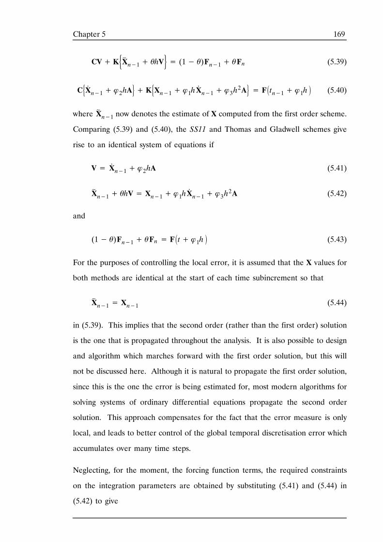
169Chapter 5
CV+KX~ n−1+ θhV = (1− θ)Fn−1+ θFn (5.39)
CX. n−1+ φ2hA +KXn−1+ φ1hX.
n−1+ φ3h2A = Ftn−1+ φ1h (5.40)
where X~n−1 now denotes the estimate of X computed from the first order scheme.
Comparing (5.39) and (5.40), the SS11 and Thomas and Gladwell schemes give
rise to an identical system of equations if
V= X.
n−1+ φ2hA (5.41)
X~n−1+ θhV= Xn−1+ φ1hX
.
n−1+ φ3h2A (5.42)
and
(1− θ)Fn−1+ θFn = F t+ φ1h (5.43)
For the purposes of controlling the local error, it is assumed that the X values for
both methods are identical at the start of each time subincrement so that
X~n−1= Xn−1 (5.44)
in (5.39). This implies that the second order (rather than the first order) solution
is the one that is propagated throughout the analysis. It is also possible to design
and algorithm which marches forward with the first order solution, but this will
not be discussed here. Although it is natural to propagate the first order solution,
since this is the one the error is being estimated for, most modern algorithms for
solving systems of ordinary differential equations propagate the second order
solution. This approach compensates for the fact that the error measure is only
local, and leads to better control of the global temporal discretisation error which
accumulates over many time steps.
Neglecting, for the moment, the forcing function terms, the required constraints
on the integration parameters are obtained by substituting (5.41) and (5.44) in
(5.42) to give
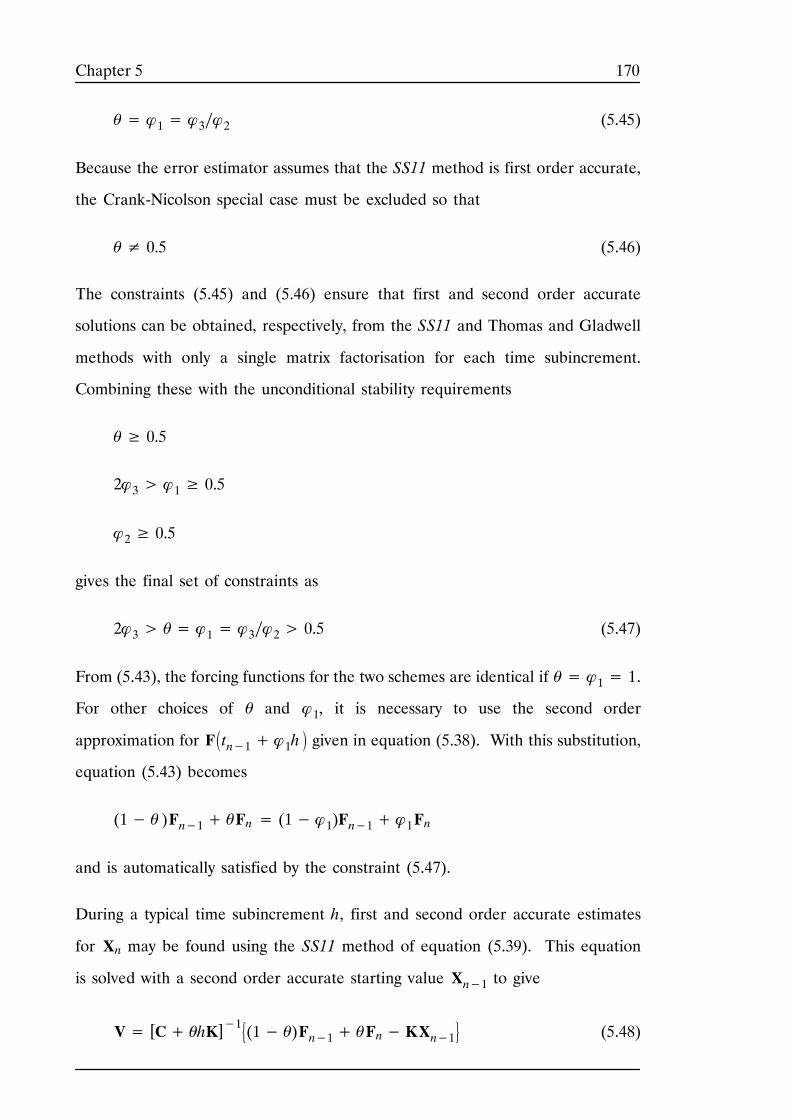
170Chapter 5
θ= φ1= φ3∕φ2 (5.45)
Because the error estimator assumes that the SS11 method is first order accurate,
the Crank-Nicolson special case must be excluded so that
θ≠ 0.5 (5.46)
The constraints (5.45) and (5.46) ensure that first and second order accurate
solutions can be obtained, respectively, from the SS11 and Thomas and Gladwell
methods with only a single matrix factorisation for each time subincrement.
Combining these with the unconditional stability requirements
θ≥ 0.5
2φ3> φ1≥ 0.5
φ2≥ 0.5
gives the final set of constraints as
2φ3> θ= φ1= φ3∕φ2> 0.5 (5.47)
From (5.43), the forcing functions for the two schemes are identical if θ= φ1= 1.
For other choices of θ and φ1, it is necessary to use the second order
approximation for Ftn−1+ φ1h given in equation (5.38). With this substitution,
equation (5.43) becomes
(1− θ )Fn−1+ θFn = (1− φ1)Fn−1+ φ1Fn
and is automatically satisfied by the constraint (5.47).
During a typical time subincrement h, first and second order accurate estimates
for Xn may be found using the SS11 method of equation (5.39). This equation
is solved with a second order accurate starting value Xn−1 to give
V= [C+ θhK]−1(1− θ)Fn−1+ θFn−KXn−1 (5.48)
171Chapter 5
with the update of (5.32) being modified to
X~n= Xn−1+ hV (5.49)
A is then found from equation (5.41)
A=V− X
.
n−1φ2h
(5.50)
where X.
n−1 is assumed known and the second order updates (5.35) and (5.36) are
Xn= Xn−1+ hX.
n−1+12 h2A (5.51)
X.n= X
.
n−1+ hA (5.52)
Since the local truncation errors in the updates (5.51) and (5.49) are, respectively,
O(h3) and O(h2), the lower order estimate may be subtracted from the higher
order estimate to give the local truncation error measure
En= Xn− X~n= hX
.
n−1+12h2A− hV
Substituting equations (5.50) and (5.52), this estimator may be expressed in the
forms
En= h1− 12φ2X. n−1+ 12φ2− 1V
or
En= hφ2− 12X. n−1+12− φ2X. n
Note that the undesirable special case of φ2= 0.5, which gives a zero estimate
of the local error regardless of h, is automatically excluded by the constraints
(5.47). For the purposes of error control, En may be replaced by the more useful
dimensionless relative error measure
172Chapter 5
Rn= max Eun Un ,EpnPn (5.53)
where
Eun= hφ2− 12U. n−1+12− φ2U. n (5.54)
Epn= hφ2− 12P. n−1+12− φ2P. nand Un and Pn are the displacement and pore pressure components of Xn and U
.n
and P.n are the velocity and pore pressure rate components of X
.n. For cases where
a weightless soil is assumed, the total pore pressures correspond to the excess pore
pressures and Pn will approach zero in later stages of consolidation. To avoid
ill-conditioning of the relative error estimator in this situation, it is preferable to
measure the error in the displacements only and replace (5.53) by
Run= max Eun Un (5.55)
This approach, which is used throughout this Thesis, is sufficiently accurate for
practical computations and removes the need to employ a combination of absolute
and relative error indicators.
Once Run has been computed for the current time substep, the procedure for
adjusting the next time substep is very similar to that outlined in Section 4.4 of
Chapter 4. The current time subincrement is accepted if Run is less than some
specified tolerance on the local truncation error, DTOL, and rejected otherwise.
In either case, the size of the next time step hn+1 is found from
hn+1= qhn
where q is a factor which is chosen to limit the predicted truncation error. Since
the truncation error for the next time subincrement, Run+1, is approximately
related to Run by
173Chapter 5
Run+1≈ q2Run
the required factor q is found by insisting that Run+1≤ DTOL to give
q≤ DTOL∕Run
As in Section 4.4, q is chosen conservatively to minimise the number of rejected
time subincrements. according to
q= 0.9 DTOL∕Run (5.56)
with the additional constraint that
0.1≤ q≤ 2 (5.57)
The safety factor coefficient of 0.9 is greater than the value of 0.7 used in the
elastoplastic load substepping scheme because the nonlinearities for elastic
consolidation are less extreme. For the same reason, the maximum value for q,
which determines the maximum size of consecutive time substeps, has been
increased from 1.1 to 2. The value of the safety factor in (5.56), and the limits
in (5.57), were determined by numerical experiments on a wide variety of
examples and ensure that most of the substeps are successful without making the
step selection mechanism too conservative. For the reasons discussed in Section
4.4, the step size is again prohibited from growing immediately after a failed time
subincrement.
Assuming initial values for h and X0, with the latter typically zero, the integration
scheme is started by solving (5.48) for V. For the first coarse time increment, h
is typically set to Δt, but in subsequent coarse time increments it may be initialised
to the value that gave the last successful subincrement. In order to compute the
second order update for X using equation (5.51), a starting value for X.at t= 0
is needed. Assuming that the matrix C has an inverse, X.
0 may be found by solving
the governing differential equation (5.27) at t= 0 according to
174Chapter 5
X.
0= [C]–1F0−KX0 (5.58)
This type of procedure is valid for elements with a pore pressure expansion which
is one order lower than the displacement expansion. For elements where the
expansions are the same, C does not have an inverse and equation (5.58) cannot
be used. The simplest alternative in this case is to take a very small time step
δh and apply equations (5.48), (5.50) and (5.52) with X0= X.
0= 0 to give
V= [C+ θδhK]−1(1− θ)F0++ θF0+
X.
0+ = V∕φ2
where the subscript 0+ indicates quantities evaluated at time t= δh. For a
sufficiently small value of δh, X.
0+ may be used as the initial value for X.at time
t= 0.
At the start of a typical substep, V is found from (5.48) and the updates for X
and X.are computed using (5.50)---(5.52). The relative error Run is then
determined using equations (5.54) and (5.55). If this error is less than or equal
to the specified tolerance DTOL, then the current time subincrement is accepted
and the step size for the next time subincrement is found using (5.56) and (5.57).
If Run exceeds DTOL, then the solution is rejected and equations (5.56) and (5.57)
are used to predict a smaller step size that will hopefully satisfy the constraint on
the local error. In this case, the stage is repeated and, if necessary, the step size
is reduced further until a successful time substep size is obtained.
The discussion has, so far, assumed that it is convenient to evaluate the external
force rate, F. ext= dFext∕dt, analytically in the overall forcing function defined by
equation (5.29). For cases where this is not so, this derivative can be approximated
using discrete values of the external force vector. Examples of four useful
approximations are
F. extn = (Fextn − F
extn−1)∕h+ 0(h) (5.59)
175Chapter 5
F. extn−1= (F
extn − F
extn−1)∕h+ 0(h) (5.60)
F. extn = (3Fextn − 4F
extn−1∕2+ F
extn−1)∕h+ 0(h
2) (5.61)
F. extn−1= (− 3F
extn−1+ 4Fextn−1∕2− F
extn )∕h+ 0(h
2) (5.62)
where h is the current time step and the subscripts n− 1, n− 1∕2, and n denote
values computed at the times tn−1, tn−1∕2= tn−1+ h∕2 and tn= tn−1+ h.
Since the adaptive integration scheme described here is second order accurate,
equations (5.61) and (5.62) should be employed when the variation of the external
forcing function is nonlinear with time. For problems where the external loading
is piecewise linear with time, which covers most practical situations, the
approximations (5.59) and (5.60) are exact and therefore appropriate. These
approximations are used throughout this Thesis.
5.5.2 Scaling of Linear Equations
The automatic solution scheme described in the previous Section requires the
solution of the linear system of equations (5.48). These may be written in the
simple form
⎪⎡⎣Ke
LT
L
θhH⎪⎤⎦⎨⎧⎩U.
P.⎬⎫⎭= ⎨⎧⎩
Ru
Rp⎬⎫⎭
(5.63)
where U.and P
.are, respectively, average velocities and pore pressure rates over
a time step h, and Ru and Rp are arbitrary vectors. For small time steps h, this
system may become ill-conditioned as the diagonal terms in K can be many orders
of magnitude greater than the terms in θhH. The effects of ill-conditioning were
first noted by Ghaboussi and Wilson (1973), who developed a criterion for
selecting a minimum value of h. This criterion is valid for consolidation of an
elastic soil which is isotropic and homogeneous. Rather than limiting the size of
the time step, which can introduce another source of error due to the time
176Chapter 5
dependence of the governing equations, it is possible to scale the various terms
in (5.63) so that ill-conditioning is avoided. This approach, suggested by Reed
(1984) and used in Lewis and Schrefler (1987), has proven successful and is
adopted in this Thesis. The scaling preserves any symmetry of the original linear
equations and takes the form
⎪⎡
⎣
K
sLT
sL
s2θhH⎪⎤
⎦⎪⎪⎨⎧
⎩
U.
1s P.⎪⎪⎬⎫
⎭= ⎪⎪⎨⎧
⎩
Ru
sRp⎪⎪⎬⎫
⎭
where s is a scalar parameter which is chosen so as to roughly equate the size of
the diagonal terms in K and s2θhH. Ignoring the effects of the element geometry,
the diagonal terms of K are proportional to the terms of the elastic stress strain
matrix D, and hence are of the order of Young’s modulus E. Similarly, the terms
of the matrix H are approximately proportional to k∕γw, where k is a
representative value of the permeability. Equating these contributions and noting
that θ is of order 1, a suitable value for the scaling parameter can be estimated
as
s=Eγwhk
For problems involving a homogeneous isotropic soil, the choice of E and k in the
above equation is straightforward. In other situations, however, it is necessary to
choose representative values of these material parameters. One such scaling
strategy can be found in the code of Lewis and Schrefler (1987).
5.5.3 Implementation
In deciding upon an implementation of the automatic integration scheme
described in Section 5.5.1, it is necessary to choose specific values of the
integration parameters θ, φ1, φ2 and φ3 which satisfy the constraints (5.47). After
a series of numerical experiments covering a wide range of problems, these were
set to
177Chapter 5
θ= φ1= φ2= φ3= 1 (5.64)
The advantages of this choice are as follows:
i) Setting θ= 1 implies that the first order method corresponds to the backward
Euler scheme. This procedure is known to damp out unwanted oscillations
quickly and thus provides a reliable first order solution for estimating the local
truncation error.
ii) Selecting φ1= θ= 1 means that the forcing functions for the first order and
second order schemes are identical without any need to make the
approximation shown in equation (5.38). Moreover, there is no need to
evaluate the forcing function outside of the current time step.
iii) Setting φ2= 1 means that the vector V, computed from equation (5.48),
corresponds automatically to X.n, the value of X
.at the end of the current step
for the second order scheme. This feature, which can be seen by comparing
equations (5.41) and (5.52), results in a compact algorithm.
Other settings for these parameters are of course possible, and may lead to a
scheme with improved performance for certain cases. The values in (5.64),
however, will be shown in the next Chapter to give excellent results for a broad
range of practical problems.
As mentioned previously, the implementation of the adaptive integration
algorithm assumes that a series of coarse time increments have been specified.
These coarse increments are, if necessary, subincremented automatically to satisfy
a tolerance on the local truncation error.
The automatic time stepping algorithm for elastic consolidation may be
summarised as follows.
1. Enter with the time at the start of the coarse increment t0, the current
displacements and pore pressures Xt0, their corresponding derivatives X.
t0,
the coarse time increment Δt, the last successful time substep hlast, the
178Chapter 5
current effective stresses at each integration point σ′t0 , and the specified
displacement error tolerance DTOL. For the first coarse time step, set
hlast= Δt.
2. Set t= t0 and h= min {hlast ,Δt }
3. While t< t0+ Δt do steps 4 to 9.
4. Compute X.
t+h according to
X.
t+h= [C+ hK]–1Ft+h−KXt
where
Ft+h=⎨⎧⎩F. extt+h
Qt+h⎬⎫⎭= ⎨⎧⎩(Fextt+h− F
extt )∕h
Q t+h⎬⎫⎭
5. Estimate the local truncation error in the displacements for the current
subincrement using
Eut+h=12hU. t− U
.
t+h
where U.denotes the velocity component of X
..
6. Update the displacements and pore water pressures and hold them in
temporary storage according to
Xt+h= Xt+h2X. t+ X
.
t+h
7. Estimate the relative error for current subincrement using
Rut+h= maxEPS , Eut+h ∕ Ut+h
where Ut+h is the displacement component of Xt+h and EPS is a machine
constant.
8. If Rut+h> DTOL then go to step 9. Else this step is successful so update
displacements, pore pressures and integration point effective stresses
according to
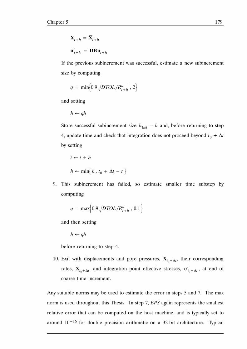
179Chapter 5
Xt+h= Xt+h
σ′t+h = DBut+h
If the previous subincrement was successful, estimate a new subincrement
size by computing
q= min0.9 DTOL∕Rut+h , 2
and setting
h← qh
Store successful subincrement size hlast= h and, before returning to step
4, update time and check that integration does not proceed beyond t0+ Δt
by setting
t← t+ h
h← min h , t0+ Δt− t
9. This subincrement has failed, so estimate smaller time substep by
computing
q= max0.9 DTOL∕Rut+h , 0.1
and then setting
h← qh
before returning to step 4.
10. Exit with displacements and pore pressures, Xt0+Δt, their corresponding
rates, X.
t0+Δt, and integration point effective stresses, σ′t0+Δt , at end of
coarse time increment.
Any suitable norms may be used to estimate the error in steps 5 and 7. The max
norm is used throughout this Thesis. In step 7, EPS again represents the smallest
relative error that can be computed on the host machine, and is typically set to
around 10---16 for double precision arithmetic on a 32-bit architecture. Typical
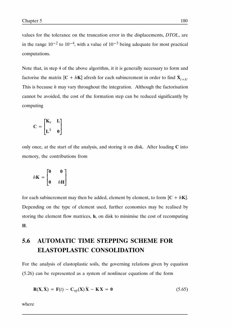
180Chapter 5
values for the tolerance on the truncation error in the displacements, DTOL, are
in the range 10---2 to 10---4, with a value of 10---3 being adequate for most practical
computations.
Note that, in step 4 of the above algorithm, it it is generally necessary to form and
factorise the matrix [C+ hK] afresh for each subincrement in order to find X.
t+h.
This is because h may vary throughout the integration. Although the factorisation
cannot be avoided, the cost of the formation step can be reduced significantly by
computing
C=⎪⎡⎣Ke
LT
L
0⎪⎤⎦
only once, at the start of the analysis, and storing it on disk. After loading C into
memory, the contributions from
hK=⎪⎡⎣0
0
0
hH⎪⎤⎦
for each subincrement may then be added, element by element, to form [C+ hK].
Depending on the type of element used, further economies may be realised by
storing the element flow matrices, h, on disk to minimise the cost of recomputing
H.
5.6 AUTOMATIC TIME STEPPING SCHEME FORELASTOPLASTIC CONSOLIDATION
For the analysis of elastoplastic soils, the governing relations given by equation
(5.26) can be represented as a system of nonlinear equations of the form
R(X,X.)= F(t)− Cep(X)X
.−KX= 0 (5.65)
where
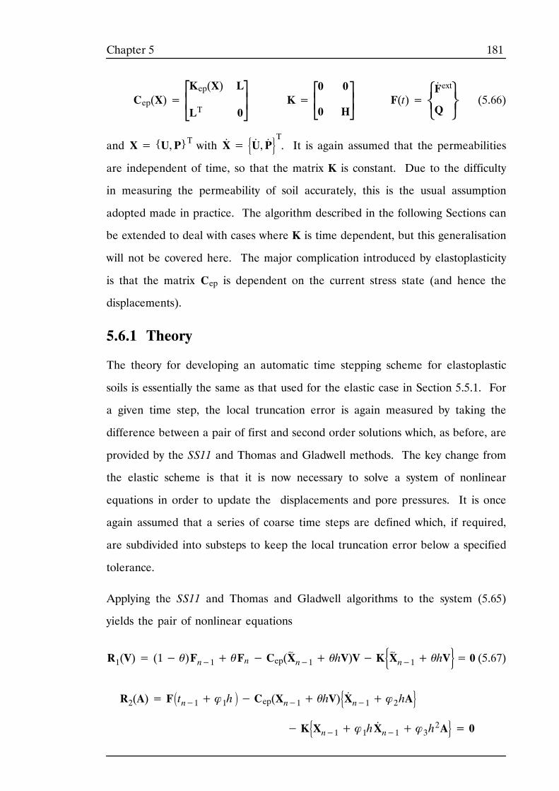
181Chapter 5
Cep(X)=⎪⎡⎣Kep(X)
LT
L
0⎪⎤⎦
K=⎪⎡⎣0
0
0
H⎪⎤⎦
F(t)=⎨⎧⎩F. ext
Q⎬⎫⎭
(5.66)
and X= {U,P}T with X.= U. ,P. T. It is again assumed that the permeabilities
are independent of time, so that the matrix K is constant. Due to the difficulty
in measuring the permeability of soil accurately, this is the usual assumption
adopted made in practice. The algorithm described in the following Sections can
be extended to deal with cases where K is time dependent, but this generalisation
will not be covered here. The major complication introduced by elastoplasticity
is that the matrix Cep is dependent on the current stress state (and hence the
displacements).
5.6.1 Theory
The theory for developing an automatic time stepping scheme for elastoplastic
soils is essentially the same as that used for the elastic case in Section 5.5.1. For
a given time step, the local truncation error is again measured by taking the
difference between a pair of first and second order solutions which, as before, are
provided by the SS11 and Thomas and Gladwell methods. The key change from
the elastic scheme is that it is now necessary to solve a system of nonlinear
equations in order to update the displacements and pore pressures. It is once
again assumed that a series of coarse time steps are defined which, if required,
are subdivided into substeps to keep the local truncation error below a specified
tolerance.
Applying the SS11 and Thomas and Gladwell algorithms to the system (5.65)
yields the pair of nonlinear equations
R1(V)= (1− θ)Fn−1+ θFn− Cep(X~n−1+ θhV)V−KX~ n−1+ θhV= 0 (5.67)
R2(A)= Ftn−1+ φ1h − Cep(Xn−1+ θhV)X.
n−1+ φ2hA
−KXn−1+ φ1hX.
n−1+ φ3h2A = 0
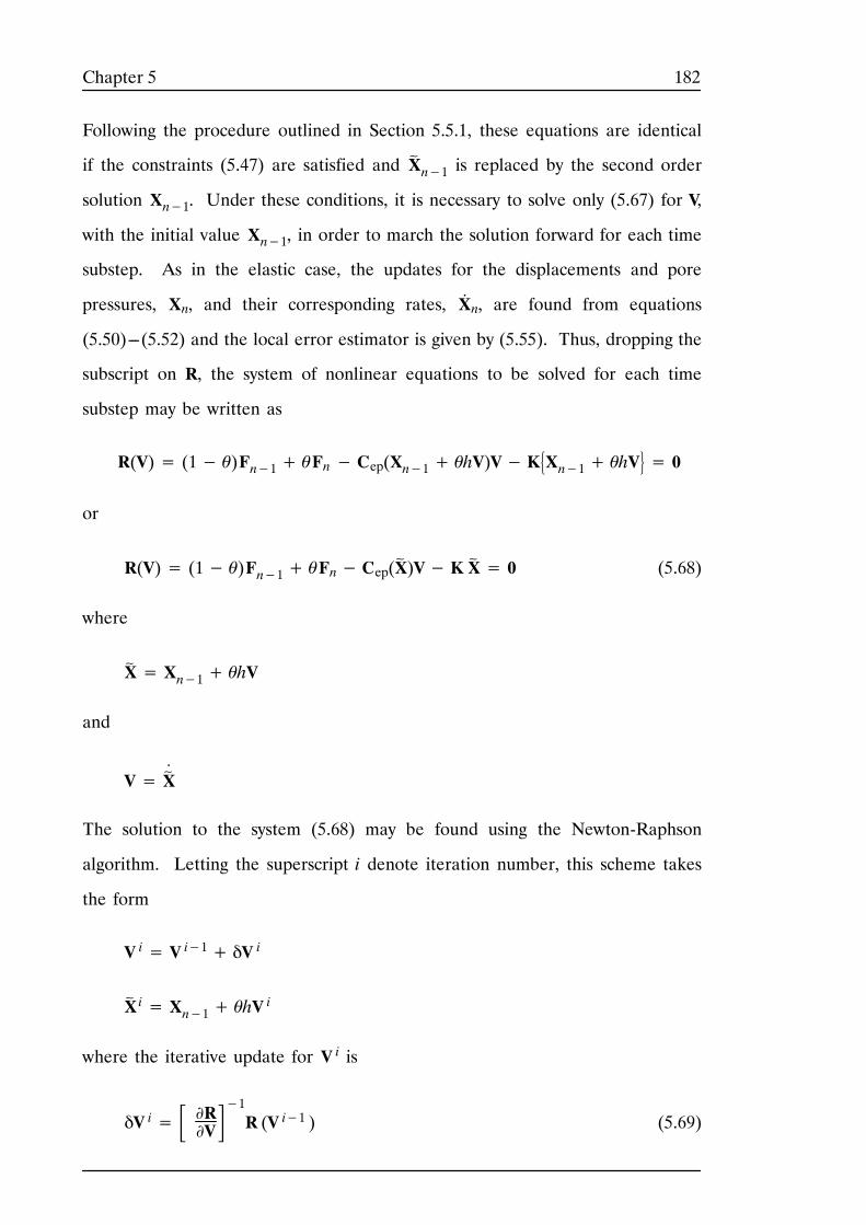
182Chapter 5
Following the procedure outlined in Section 5.5.1, these equations are identical
if the constraints (5.47) are satisfied and X~n−1 is replaced by the second order
solution Xn−1. Under these conditions, it is necessary to solve only (5.67) for V,
with the initial value Xn−1, in order to march the solution forward for each time
substep. As in the elastic case, the updates for the displacements and pore
pressures, Xn, and their corresponding rates, X.n, are found from equations
(5.50)---(5.52) and the local error estimator is given by (5.55). Thus, dropping the
subscript on R, the system of nonlinear equations to be solved for each time
substep may be written as
R(V)= (1− θ)Fn−1+ θFn− Cep(Xn−1+ θhV)V−KXn−1+ θhV = 0
or
R(V)= (1− θ)Fn−1+ θFn− Cep(X~)V− K X~ = 0 (5.68)
where
X~ = Xn−1+ θhV
and
V= X~.
The solution to the system (5.68) may be found using the Newton-Raphson
algorithm. Letting the superscript i denote iteration number, this scheme takes
the form
V i= V i−1+ δV i
X~ i= Xn−1+ θhV
i
where the iterative update for V i is
δV i= ∂R∂V−1R (V i−1 ) (5.69)
183Chapter 5
and the Jacobian matrix ∂R∕∂V is evaluated at X~ i−1. Suitable values for starting
the iterations may be obtained by setting
V 0= X.
n−1
X~ 0= Xn−1+ θhX
.
n−1
To complete the description of the Newton-Raphson algorithm, it is necessary to
evaluate ∂R∕∂V. Differentiating (5.68) and neglecting second derivatives with
respect to V gives the required Jacobian matrix as
∂R∂V = Cep(X~ )+ θhK (5.70)
Note that if the Kep component of Cep is formed using the Dep defined by (2.10),
then this Jacobian matrix is only an approximation to ∂R∕∂V and the rate of
convergence of the iteration scheme will be linear rather than quadratic. With the
proposed integration method, however, the number of iterations required for a
typical time substep is usually low due to the fact that the error control mechanism
automatically chooses small time steps in the vicinity of highly nonlinear
behaviour. At the cost of introducing complexity, quadratic convergence may be
obtained by using the so-called ‘consistent’ form of Dep introduced by Simo and
Taylor (1985). For cases which are only mildly nonlinear, it is possible to replace
(5.70) by the initial stiffness approximation
∂R∂V ≈ [C+ θhK]
where C is given by (5.28). Although much slower to converge, this approach does
not require a fresh factorisation for each iteration and always has a well
conditioned Jacobian matrix.
A convenient check for terminating the iteration procedure is to test whether the
relative change in the displacement component of X~is less than or equal to a
specified tolerance, ITOL. This can be expressed as
184Chapter 5
θhδU~. iU~ i ≤ ITOL
where U~corresponds to the displacement entries in X
~and U
~.
corresponds to the
velocity entries in V.
Depending on the values of the integration parameter θ, a number of alternative
strategies can be used to evaluate the residual R (V i−1 ) in equation (5.69). The
various options available become evident upon substituting equations (5.66) in
(5.68) to give the expanded form
R(V i−1 )= ⎪⎪⎨⎧
⎩
(1− θ)F. extn−1+ θF
. extn
(1− θ)Qn−1+ θQn⎪⎪⎬⎫
⎭−⎪⎪⎡
⎣
Kep(X~n)
LT
L
0
⎪⎪⎤
⎦⎪⎪⎨⎧
⎩
U~.i−1
P~.i−1⎪⎪⎬⎫
⎭
−⎪⎪⎡
⎣
0
0
0
H⎪⎪⎤
⎦⎪⎪⎨⎧
⎩
U~ i−1
P~ i−1⎪⎪⎬⎫
⎭
For values of the integration parameter in the range 0.5< θ< 1, it is easiest to
work with an analytic form for F. ext and perform the remaining matrix-vector
multiplications element by element.
For the backward Euler case where θ= 1, V and X~ contain values at the end of
the current time step and the residual becomes
R(V i−1n )= ⎪⎪⎨⎧
⎩
F. extn
Qn⎪⎪⎬⎫
⎭−⎪⎪⎪⎡
⎣
Kep(X~n)
LT
L
0
⎪⎪⎪⎤
⎦⎪⎪⎨⎧
⎩
U~.i−1n
P~.i−1n⎪⎪⎬⎫
⎭−⎪⎪⎪
⎡
⎣
0
0
0
H
⎪⎪⎪
⎤
⎦⎪⎪⎨⎧
⎩
U~ i−1n
P~ i−1n
⎪⎪⎬⎫
⎭
Noting that
F. intn =
V
BTσ. n dV= Kep(X~n)U~. i−1n + LP~
.i−1n
185Chapter 5
and using the first order approximations
F. intn = (F intn − F
intn−1)∕h+ 0(h)
F. extn = (F extn − F
extn−1)∕h+ 0(h)
this may written in the alternative form
R(V i−1n )= ⎪⎪⎨⎧
⎩
Fextn − Fintnh
Qn⎪⎪⎬⎫
⎭−⎪⎪⎨⎧
⎩
Fextn−1− Fintn−1
h
0⎪⎪⎬⎫
⎭−⎪⎪⎡
⎣
0
LT
0
H
⎪⎪⎤
⎦⎪⎪⎨⎧
⎩
U~.i−1n
P~ i−1n⎪⎪⎬⎫
⎭(5.71)
The first two terms on the right hand side of the above equation arise, respectively,
from the unbalanced forces at the end and the start of the time substep. Provided
the iteration tolerance ITOL is sufficiently small, the latter forces will be negligible
so that
F. unbn−1= (F
extn−1− F
intn−1)∕h≈ 0
Under these circumstances, equilibrium will also be satisfied at the end of the time
substep since the Newton-Raphson iterations enforce the condition
F. unbn = (Fextn − Fintn )∕h≈ 0 (5.72)
If ITOL is less stringent, so that the unbalanced forces at the start of the time
substep are not small, then the solution will tend to drift from equilibrium as it
is marched forward. Since the solution will be more accurate if equilibrium is
obeyed, it is always desirable to enforce the condition (5.72). This implies that
(5.71) may be replaced by
R(V i−1n )= ⎪⎪⎨⎧
⎩
Fextn − Fintnh
Qn⎪⎪⎬⎫
⎭−⎪⎪⎡
⎣
0
LT
0
H
⎪⎪⎤
⎦⎪⎪⎨⎧
⎩
U~.i−1n
P~ i−1n⎪⎪⎬⎫
⎭
To complete the residual evaluation for the case in which θ= 1, the matrix
multiplications
186Chapter 5
LT U~.i−1n
and
H P~ i−1n
may be performed element by element.
Once the solution for V has been obtained for each time substep, the error control
and step adjustment mechanism is almost identical to that discussed in Section
5.5.1. The only minor change is that the safety factor in (5.56) is lowered from
0.9 to 0.8 so that
q= 0.8 DTOL∕Run
This means the step control mechanism is slightly more conservative than that for
the elastic case, and allows for the material nonlinearity introduced by
elastoplasticity.
5.6.2 Implementation
The nonlinear automatic time stepping scheme developed in the previous Section
can be implemented in the same manner as the linear elastic scheme described
in Section 5.5.3. It is again assumed that a number of coarse time increments are
defined which, if necessary, are automatically subincremented so that the local
truncation error for each substep does not exceed a prescribed tolerance, DTOL.
Because of the advantages discussed in Section 5.5.3, the integration parameters
are again chosen to be
θ= φ1= φ2= φ3= 1
The automatic time stepping algorithm for elastoplastic consolidation may be
summarised as follows.
1. Enter with the time at the start of the coarse increment t0, the current
displacements and pore pressures Xt0, their corresponding derivatives X.
t0,
187Chapter 5
the coarse time increment Δt, the last successful time substep hlast, the
current stress state at each integration point (σ′t0 , Àt0), the iteration
tolerance ITOL, and the specified displacement error tolerance DTOL. For
the first coarse time step, set hlast= Δt.
2. Set t= t0 and h= min {hlast ,Δt }
3. While t< t0+ Δt do steps 4 to 8
4. Compute X.
t+h and X~
t+h using the Newton---Raphson or initial stiffness
algorithm. If the solution fails to converge, set
h← 0.25h
and try again.
5. Estimate the local truncation error in the displacements for the current
subincrement using
Eut+h=12hU. t− U
.
t+h
where U.denotes the velocity component of X
..
6. Estimate the relative error for current subincrement using
Rut+h= maxEPS , Eut+h ∕ U~ t+h where U
~
t+h is the displacement component of X~
t+h and EPS is a machine
constant.
7. If Rut+h> DTOL then go to step 8. Else this step is successful so compute
new displacements and pore pressures using the second order update
Xt+h= Xt+h2X. t+ X
.
t+h
For each integration point, compute the strains
Δε= Bh2 u. t+ u. t+hand integrate constitutive law to find corresponding increments in stresses,
Δσ′, and hardening parameter ΔÀ. Then update stress state according to
188Chapter 5
σ′t+h = σ′t + Δσ′
Àt+h= Àt+ ΔÀ
If the previous subincrement was successful, estimate a new subincrement
size by computing
q= min0.8 DTOL∕Rut+h , 2
and then setting
h← qh
Store successful subincrement size hlast= h and, before returning to step
4, update time and check that integration does not proceed beyond t0+ Δt
by setting
t← t+ h
h← min h , t0+ Δt− t
8. This subincrement has failed, so estimate smaller time subincrement by
computing
q= max0.8 DTOL∕Rut+h , 0.1
and then setting
h← qh
before returning to step 4.
9. Exit with displacements and pore pressures, Xt0+Δt, their corresponding
rates, X.
t0+Δt, and integration point stress state, (σ′t0+Δt , Àt0+Δt ), at end of
coarse time increment.
The Newton-Raphson procedure for solving the solving the nonlinear equations
(5.68) may be summarised as
1. Enter with the current displacements and pore pressures Xt, their
corresponding derivatives X.
t, the current step size h, the iteration tolerance
ITOL, and the maximum number of iterations MAXITS.
189Chapter 5
2. Compute estimate of new displacements/pore pressures and their
corresponding rates using
X~ 0t+h= Xt+ hX
.
t
X. 0t+h= X
.
t
3. Set
α0= hU. t ∕ U~ 0t+h where U
.
t is the velocity component of X.
t and U~ 0t+h is the displacement
component of X~ 0t+h.
4. Repeat steps 5 to 8 for i=1 to MAXITS
5. Compute residual vector
Ri=⎪⎪⎨⎧
⎩
Fextt+h− F
intt+h
h
Qt+h⎪⎪⎬⎫
⎭−⎪⎪⎡
⎣
0
LT
0
H
⎪⎪⎤
⎦⎪⎪⎨⎧
⎩
U. i−1t+h
P~ i−1t+h⎪⎪⎬⎫
⎭
and solve for δX. i using
δX. i= Cep+ hK
−1Ri (tangent stiffness)
or
δX. i= [C+ hK]−1Ri (initial stiffness)
where Fintt+h and Cep are evaluated at X~ i−1t+h.
6. Update the displacements and pore pressures and their rates
according to
X. it+h= X
. i−1t+h+ δX
. i
X~ it+h= Xt+ hX
. it+h
7. Compute convergence criterion
αi= hδU. i ∕ U~ it+h
190Chapter 5
where δU. i is the velocity component of δX
. i and U~ it+h is the
displacement component of X~ it+h. If α
i< ITOL then go to step 10.
8. For tangent stiffness only, check rate of convergence. If αi∕αi−1> 0.5
for more than 2 consecutive iterations then exit with “no convergence”
warning.
9. Maximum number of iterations exceeded. Exit with “no convergence”
warning.
10. Exit with displacements/pore pressures, X~
t+h= X~ it+h, and their rates,
X.
t+h= X. it+h, at time t+h.
Typical values for the iteration tolerance, ITOL, are in the range 10---3 to 10---6,
with the lower limit ensuring that the drift from equilibrium is very small. The
maximum number of iterations permitted for each subincrement, MAXITS, is
typically set to around 15. To minimise the high cost associated with failed
substeps, and to allow for possible divergence of the iteration scheme, h is
automatically reduced by a factor of four if no convergence is obtained within this
limit. This feature may result in an excessive number of substeps if MAXITS is
set to a very low value. The optimum setting for MAXITS is dependent on the
specified value of DTOL, since loose values of this tolerance may give large time
steps and hence large numbers of iterations. It is also a function of the solution
scheme used to solve the governing nonlinear equations. The tangent stiffness
algorithm generally requires far fewer iterations than the initial stiffness algorithm,
especially if the behaviour is highly nonlinear.
For the initial stiffness method, the matrix [C+ hK] needs to be formed and
factorised afresh only once per subincrement to obtain the iterates δX. i. The cost
associated with each formation phase may be reduced significantly using the
procedure outlined in Section 5.5.3. With the tangent stiffness Newton-Raphson
scheme it is necessary to reform and refactorise the Jacobian matrix [Cep+ hK]
once per iteration, since Cep is dependent on the displacements held in X~ i−1t+h.
191Chapter 5
In this case, it is possible to exploit the strategy discussed previously in Section
4.4.3. Using the decomposition
Cep=⎪⎡⎣Kep
LT
L
0⎪⎤⎦= C− Cp=⎪⎡⎣
Ke
LT
L
0⎪⎤⎦−⎪⎡⎣Kp
0
0
0⎪⎤⎦
it is evident that the matrix C need only be formed once and stored on disk. In
order to generate Cep efficiently for each iteration, C is loaded into memory from
disk and the plastic element stiffness matrices kp, defined by (4.20), are subtracted
element by element. Since only plastic Gauss points contribute to Kp, the effort
required to form Kep, and hence Cep, is usually small for much of the loading
range.
Finally, it is also possible to hold the Jacobian matrix constant for several
subincrements and only refactorise it when convergence becomes slow or when the
step size h changes significantly. These options have not been pursued in this
Thesis, but may lead to reductions in the overall CPU time.

192Chapter 5
193Chapter 6
CHAPTER 6
CONSOLIDATION APPLICATIONS
194Chapter 6
6.1 INTRODUCTION
In this Chapter, the automatic time stepping algorithms developed in Chapter 5
are used to study the behaviour of several problems involving the consolidation
of porous media. The aim of these analyses is to demonstrate that the new
procedures:
¯ Can control the global temporal discretisation (or time-stepping) error in the
displacements to lie near a prescribed error tolerance.
¯ Automatically choose a suitable number of time subincrements to achieve the
desired accuracy, regardless of the number of coarse time increments that are
specified initially.
¯ Are robust and efficient.
The first part of this Chapter considers the consolidation of porous elastic media.
Analyses are performed for the consolidation of a layer under one dimensional
loading, the consolidation of a layer between two rigid plates, and the
consolidation of a flexible strip footing resting on a layer of finite depth. In these
examples, the performance of the automatic algorithm is investigated using various
numbers of coarse time increments and a range of error tolerances. Where
appropriate, the efficiency of the automatic algorithm is measured against the
efficiency of the conventional backward Euler method by comparing the CPU
times required to generate solutions of comparable accuracy. To gauge the ability
of the new algorithm to control the level of temporal discretisation error, the
results from the automatic scheme are compared against those from a second
order accurate scheme using very small time steps. The latter solutions contain
negligible temporal discretisation errors, and thus serve as useful benchmarks.
Note that no attempt is made to measure the spatial discretisation error, which
is governed by the mesh configuration.
The next part of this Chapter investigates the ability of the elastoplastic
consolidation formulation to predict drained and undrained failure modes in a soil
195Chapter 6
mass. These cases illustrate two extremes of consolidation behaviour and are thus
useful checks on the accuracy of the finite element technique. The problems used
in these analyses are the expansion of a thick cylinder and the collapse of a flexible
strip footing.
The final part of the Chapter considers the consolidation of a flexible strip footing
resting on an elastoplastic soil layer. The layer is modelled using a rounded
Mohr-Coulomb yield surface with either an associated or a nonassociated flow
rule. For both the associated and nonassociated cases where where the dilation
angle is nonzero, the automatic time integration procedure is implemented using
a Newton-Raphson (or tangent stiffness) iteration scheme to solve the nonlinear
incremental equations for each time step. For the special case of a nonassociated
model with a zero dilation angle, an initial stiffness iteration scheme is employed
to solve these equations. As in the elastic consolidation examples, the results from
the automatic scheme are compared with those from the conventional backward
Euler scheme to assess its accuracy and efficiency. These analyses are also used
to investigate the effect of the iteration tolerance on the accuracy of the
displacements at various stages of consolidation.
In each of the problems to be analysed, whether elastic or elastoplastic, the soil
mass is modelled using six-noded triangles with a quadratic displacement
expansion for the displacements and a linear expansion for the pore water
pressures. This element avoids the spurious oscillations associated with elements
which use the same order of expansion for the displacements and pore pressures
(see, for example, Reed, 1984 and Kanok-Nukulchal and Suaris, 1982) and is
simple to implement.
For all problems considered in this Chapter, a ramp loading is imposed over the
time period t0 as shown in Figure 6.1. Following conventional practice, the rate
of loading is frequently expressed in terms of the time factor Tv, rather than the
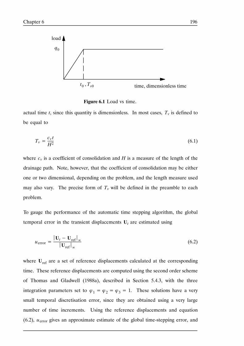
196Chapter 6
t0 , Tv0
load
time, dimensionless time
Figure 6.1 Load vs time.
q0
actual time t, since this quantity is dimensionless. In most cases, Tv is defined to
be equal to
Tv=cv tH2
(6.1)
where cv is a coefficient of consolidation and H is a measure of the length of the
drainage path. Note, however, that the coefficient of consolidation may be either
one or two dimensional, depending on the problem, and the length measure used
may also vary. The precise form of Tv will be defined in the preamble to each
problem.
To gauge the performance of the automatic time stepping algorithm, the global
temporal error in the transient displacements Ut are estimated using
uerror=Ut− Uref ∞Uref ∞
(6.2)
where Uref are a set of reference displacements calculated at the corresponding
time. These reference displacements are computed using the second order scheme
of Thomas and Gladwell (1988a), described in Section 5.4.3, with the three
integration parameters set to φ1= φ2= φ3= 1. These solutions have a very
small temporal discretisation error, since they are obtained using a very large
number of time increments. Using the reference displacements and equation
(6.2), uerror gives an approximate estimate of the global time-stepping error, and
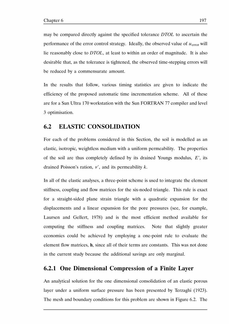
197Chapter 6
may be compared directly against the specified tolerance DTOL to ascertain the
performance of the error control strategy. Ideally, the observed value of uerror will
lie reasonably close to DTOL, at least to within an order of magnitude. It is also
desirable that, as the tolerance is tightened, the observed time-stepping errors will
be reduced by a commensurate amount.
In the results that follow, various timing statistics are given to indicate the
efficiency of the proposed automatic time incrementation scheme. All of these
are for a Sun Ultra 170 workstation with the Sun FORTRAN 77 compiler and level
3 optimisation.
6.2 ELASTIC CONSOLIDATION
For each of the problems considered in this Section, the soil is modelled as an
elastic, isotropic, weightless medium with a uniform permeability. The properties
of the soil are thus completely defined by its drained Youngs modulus, E′, its
drained Poisson’s ration, ν′, and its permeability k.
In all of the elastic analyses, a three-point scheme is used to integrate the element
stiffness, coupling and flow matrices for the six-noded triangle. This rule is exact
for a straight-sided plane strain triangle with a quadratic expansion for the
displacements and a linear expansion for the pore pressures (see, for example,
Laursen and Gellert, 1978) and is the most efficient method available for
computing the stiffness and coupling matrices. Note that slightly greater
economies could be achieved by employing a one-point rule to evaluate the
element flow matrices, h, since all of their terms are constants. This was not done
in the current study because the additional savings are only marginal.
6.2.1 One Dimensional Compression of a Finite Layer
An analytical solution for the one dimensional consolidation of an elastic porous
layer under a uniform surface pressure has been presented by Terzaghi (1923).
The mesh and boundary conditions for this problem are shown in Figure 6.2. The
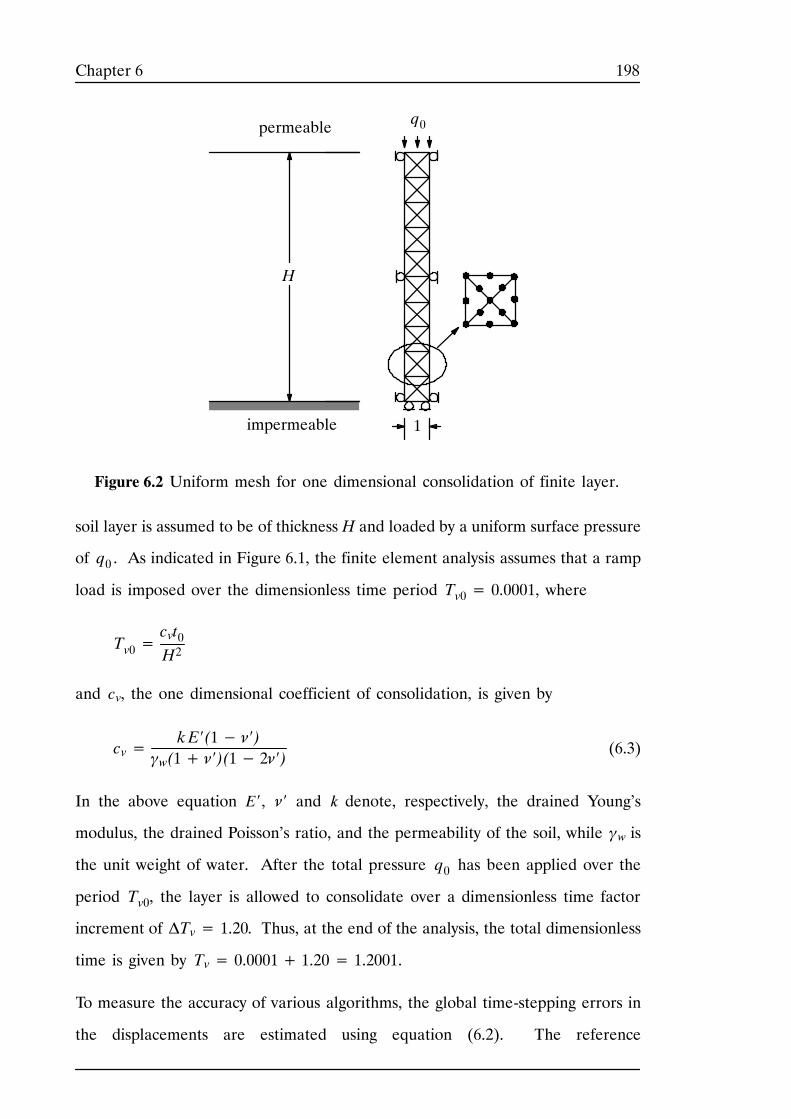
198Chapter 6
H
1
Figure 6.2 Uniform mesh for one dimensional consolidation of finite layer.
impermeable
permeable q0
soil layer is assumed to be of thickness H and loaded by a uniform surface pressure
of q0 . As indicated in Figure 6.1, the finite element analysis assumes that a ramp
load is imposed over the dimensionless time period Tv0= 0.0001, where
Tv0=cvt0H2
and cv, the one dimensional coefficient of consolidation, is given by
cv=kE′(1− ν′)
γw(1+ ν′)(1− 2ν′)(6.3)
In the above equation E′, ν′ and k denote, respectively, the drained Young’s
modulus, the drained Poisson’s ratio, and the permeability of the soil, while γw is
the unit weight of water. After the total pressure q0 has been applied over the
period Tv0, the layer is allowed to consolidate over a dimensionless time factor
increment of ΔTv= 1.20. Thus, at the end of the analysis, the total dimensionless
time is given by Tv= 0.0001+ 1.20= 1.2001.
To measure the accuracy of various algorithms, the global time-stepping errors in
the displacements are estimated using equation (6.2). The reference
199Chapter 6
displacements for this case are calculated using the second order accurate scheme
of Thomas and Gladwell (1988a), with 1000 equal size increments to apply the
load and 10,000 equal size time increments to model the subsequent consolidation.
DTOLNo. coarse time No. time subincrements* CPU
DTOLNo. coarse timeincrements* Successful Failed
CPUtime (s)
10---2 1+1=2 9+48=57 2+3=5 1.1
1+6=7 9+50=59 2+3=5 1.51+12=13 9+53=62 2+3=5 1.9
10---3 1+1=2 27+129=156 4+3=7 2.6
1+6=7 27+133=160 4+3=7 2.91+12=13 27+133=160 4+3=7 3.2
10---4 1+1=2 85+379=464 5+3=8 7.0
1+6=7 85+382=467 5+3=8 7.3
1+12=13 85+386=471 5+3=8 7.5
Table 6.1 Results for one dimensional consolidation using automatic scheme.(* no. in loading stage + no. in consolidation stage = total no.)
Results for analyses using the automatic time stepping scheme of Section 5.5.3 are
shown in Table 6.1, Figure 6.3 and Figure 6.4. Data are presented for
DTOL=10---2, 10---3 and 10---4, which are typical of the tolerance values that would
be used in practice. To test the sensitivity of the automatic scheme to the starting
conditions, three runs are performed for each tolerance using 2, 7 and 13 coarse
time steps. In each case, all of the load is applied in the first coarse time step
which has a time factor increment of ΔTv0= 0.0001. The remaining coarse
increments are of uniform size and apply a total time factor increment of
ΔTv= 1.2. Note that entries in Table 6.1 of the form i+j=k indicate that i steps
occurred in the loading phase, j steps occurred in the consolidation phase, and k
steps occurred overall.
Figure 6.3 compares the numerical consolidation curve, obtained using the
automatic scheme with 2 coarse time steps and DTOL=10---2, against the analytical
solution derived by Terzaghi (1923). This analysis generates a total of 56 substeps
and its predictions are in excellent agreement with the exact results.
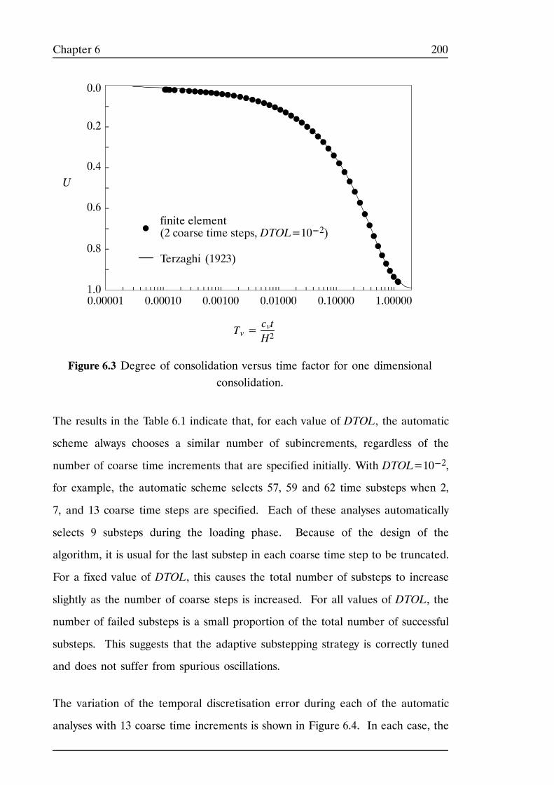
200Chapter 6
0.00001 0.00010 0.00100 0.01000 0.10000 1.00000
Figure 6.3 Degree of consolidation versus time factor for one dimensionalconsolidation.
U
Tv=cvtH2
Terzaghi (1923)
0.2
0.4
0.6
0.8
1.0
0.0
finite element(2 coarse time steps, DTOL=10---2)
The results in the Table 6.1 indicate that, for each value of DTOL, the automatic
scheme always chooses a similar number of subincrements, regardless of the
number of coarse time increments that are specified initially. With DTOL=10---2,
for example, the automatic scheme selects 57, 59 and 62 time substeps when 2,
7, and 13 coarse time steps are specified. Each of these analyses automatically
selects 9 substeps during the loading phase. Because of the design of the
algorithm, it is usual for the last substep in each coarse time step to be truncated.
For a fixed value of DTOL, this causes the total number of substeps to increase
slightly as the number of coarse steps is increased. For all values of DTOL, the
number of failed substeps is a small proportion of the total number of successful
substeps. This suggests that the adaptive substepping strategy is correctly tuned
and does not suffer from spurious oscillations.
The variation of the temporal discretisation error during each of the automatic
analyses with 13 coarse time increments is shown in Figure 6.4. In each case, the
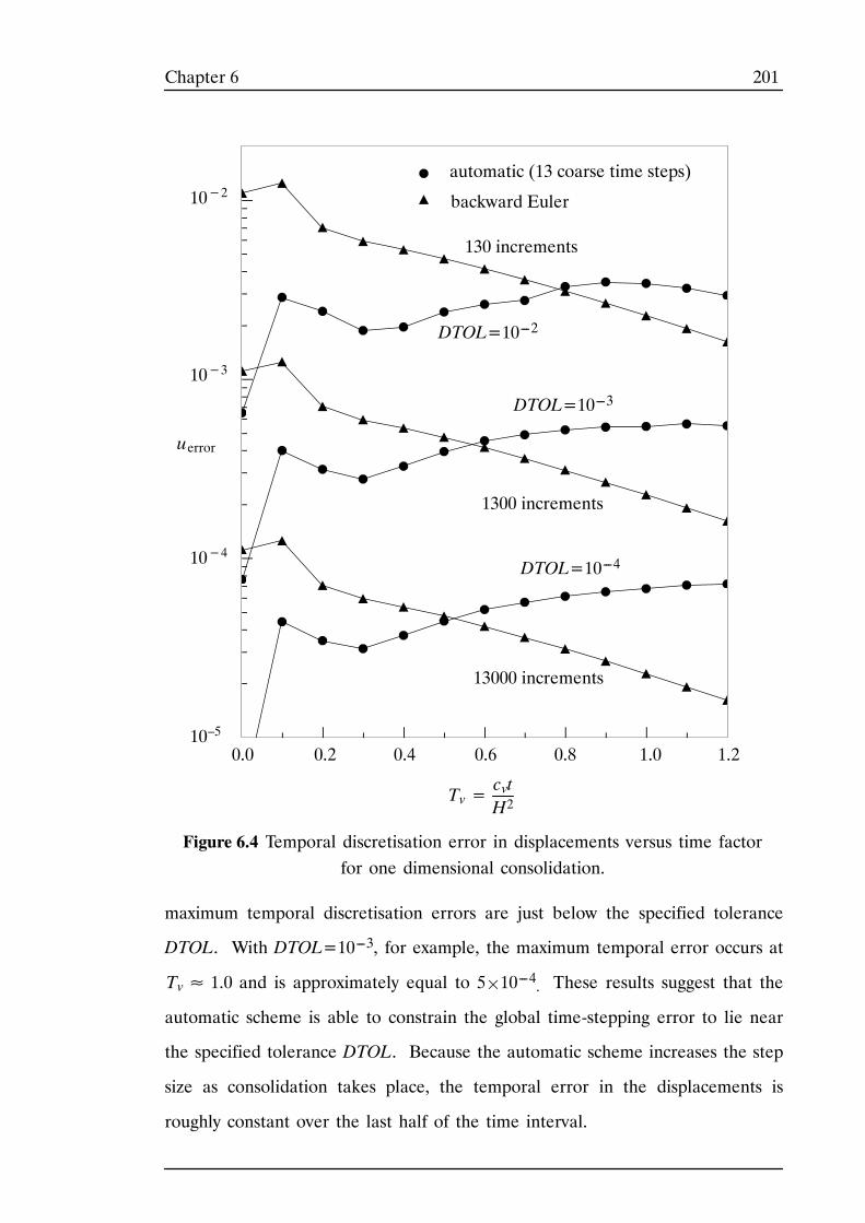
201Chapter 6
DTOL=10---2
Figure 6.4 Temporal discretisation error in displacements versus time factorfor one dimensional consolidation.
1300 increments
130 increments
automatic (13 coarse time steps)
backward Euler
DTOL=10---3
DTOL=10---4
13000 increments
Tv=cvtH2
10−2
10−3
10−4
0.0 0.2 0.4 0.6 0.8 1.0 1.2
uerror
10–5
maximum temporal discretisation errors are just below the specified tolerance
DTOL. With DTOL=10---3, for example, the maximum temporal error occurs at
Tv≈ 1.0 and is approximately equal to 5¢10---4. These results suggest that the
automatic scheme is able to constrain the global time-stepping error to lie near
the specified tolerance DTOL. Because the automatic scheme increases the step
size as consolidation takes place, the temporal error in the displacements is
roughly constant over the last half of the time interval.
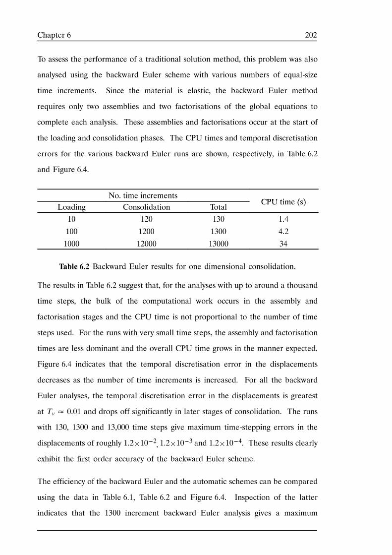
202Chapter 6
To assess the performance of a traditional solution method, this problem was also
analysed using the backward Euler scheme with various numbers of equal-size
time increments. Since the material is elastic, the backward Euler method
requires only two assemblies and two factorisations of the global equations to
complete each analysis. These assemblies and factorisations occur at the start of
the loading and consolidation phases. The CPU times and temporal discretisation
errors for the various backward Euler runs are shown, respectively, in Table 6.2
and Figure 6.4.
No. time incrementsCPU time (s)
Loading Consolidation TotalCPU time (s)
10 120 130 1.4
100 1200 1300 4.2
1000 12000 13000 34
Table 6.2 Backward Euler results for one dimensional consolidation.
The results in Table 6.2 suggest that, for the analyses with up to around a thousand
time steps, the bulk of the computational work occurs in the assembly and
factorisation stages and the CPU time is not proportional to the number of time
steps used. For the runs with very small time steps, the assembly and factorisation
times are less dominant and the overall CPU time grows in the manner expected.
Figure 6.4 indicates that the temporal discretisation error in the displacements
decreases as the number of time increments is increased. For all the backward
Euler analyses, the temporal discretisation error in the displacements is greatest
at Tv≈ 0.01 and drops off significantly in later stages of consolidation. The runs
with 130, 1300 and 13,000 time steps give maximum time-stepping errors in the
displacements of roughly 1.2¢10---2, 1.2¢10---3 and 1.2¢10---4. These results clearly
exhibit the first order accuracy of the backward Euler scheme.
The efficiency of the backward Euler and the automatic schemes can be compared
using the data in Table 6.1, Table 6.2 and Figure 6.4. Inspection of the latter
indicates that the 1300 increment backward Euler analysis gives a maximum
203Chapter 6
temporal discretisation error which is close to that of the automatic analysis with
DTOL=10---3. The data in Table 6.2 and Table 6.1 reveal that the CPU times for
these two runs are, respectively, 4.2 and 3.2 seconds. For the most accurate
analysis with DTOL=10---4, the automatic scheme generates a total of 471 substeps
and requires a maximum of 7.5 seconds of CPU time. This compares very
favourably with the 13000 increment backward Euler run, whose result is of similar
accuracy but uses 34 seconds of CPU time. It could be argued that it is
inappropriate to compare the automatic scheme against the backward Euler
method with fixed increment sizes, and that a better performance measure would
be obtained by using the latter method with varying increment sizes. The problem
then, though, is how to choose the optimal size and distribution of time increments
for the backward Euler scheme. In practice, it may be necessary to perform
several analyses in order to ascertain an efficient time stepping sequence. The
automatic scheme overcomes this difficulty, since it requires only a single analysis
to obtain a solution whose accuracy is known approximately.
The analyses shown in Table 6.1 which use just one coarse time increment for the
loading phase and one coarse time increment for the consolidation phase are
included to highlight the robustness of the proposed algorithm. A bar chart of the
successful substeps chosen by the automatic scheme, for the case of DTOL=10---2,
is presented in Figure 6.5. This indicates that the time step grows by almost five
orders of magnitude, from an initial value of Tv≈ 5× 10⁻⁶ to a maximum value
of Tv≈ 0.17. As expected, the automatic scheme selects very small increments
in the early stages of the analysis where the rate of pore pressure dissipation is
the greatest. Using a log-log plot of the increment size ΔTv versus Tv, the growth
in step size for all of the automatic runs is shown in Figure 6.6. The dramatic
increases indicated in this plot highlight the inefficiency of using uniform time
steps for this particular problem, and further demonstrates the benefits obtained
by the use of an adaptive integration scheme.
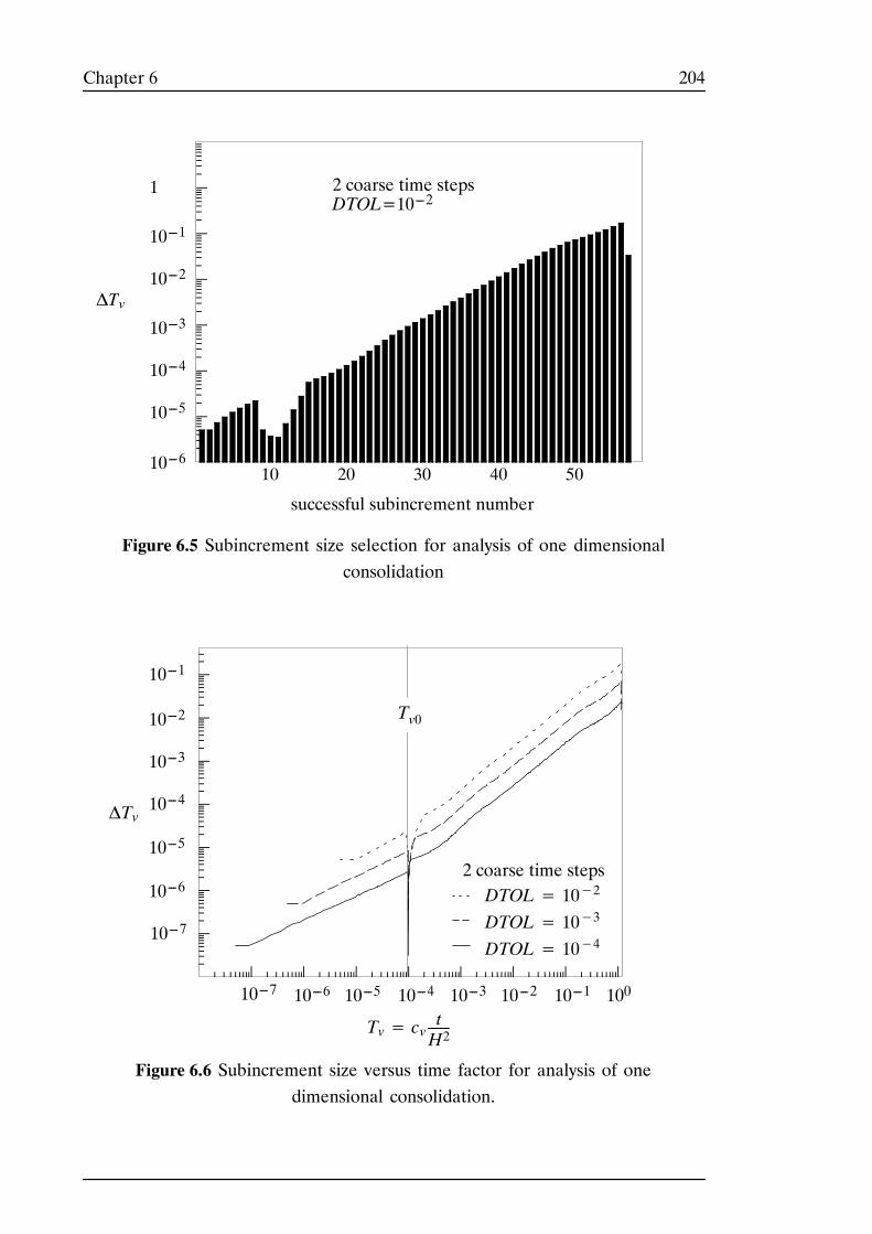
204Chapter 6
Figure 6.5 Subincrement size selection for analysis of one dimensionalconsolidation
10 20 30 40 50
successful subincrement number
ΔTv
2 coarse time stepsDTOL=10---2
10---1
10---2
10---3
10---4
10---5
1
10---6
Figure 6.6 Subincrement size versus time factor for analysis of onedimensional consolidation.
ΔTv
Tv= cv tH2
10010---110---210---4 10---310---510---6
10---1
10---2
10---3
10---4
10---5
10---6
Tv0
DTOL= 10−4DTOL= 10−3DTOL= 10−2
2 coarse time steps
10---7
10---7
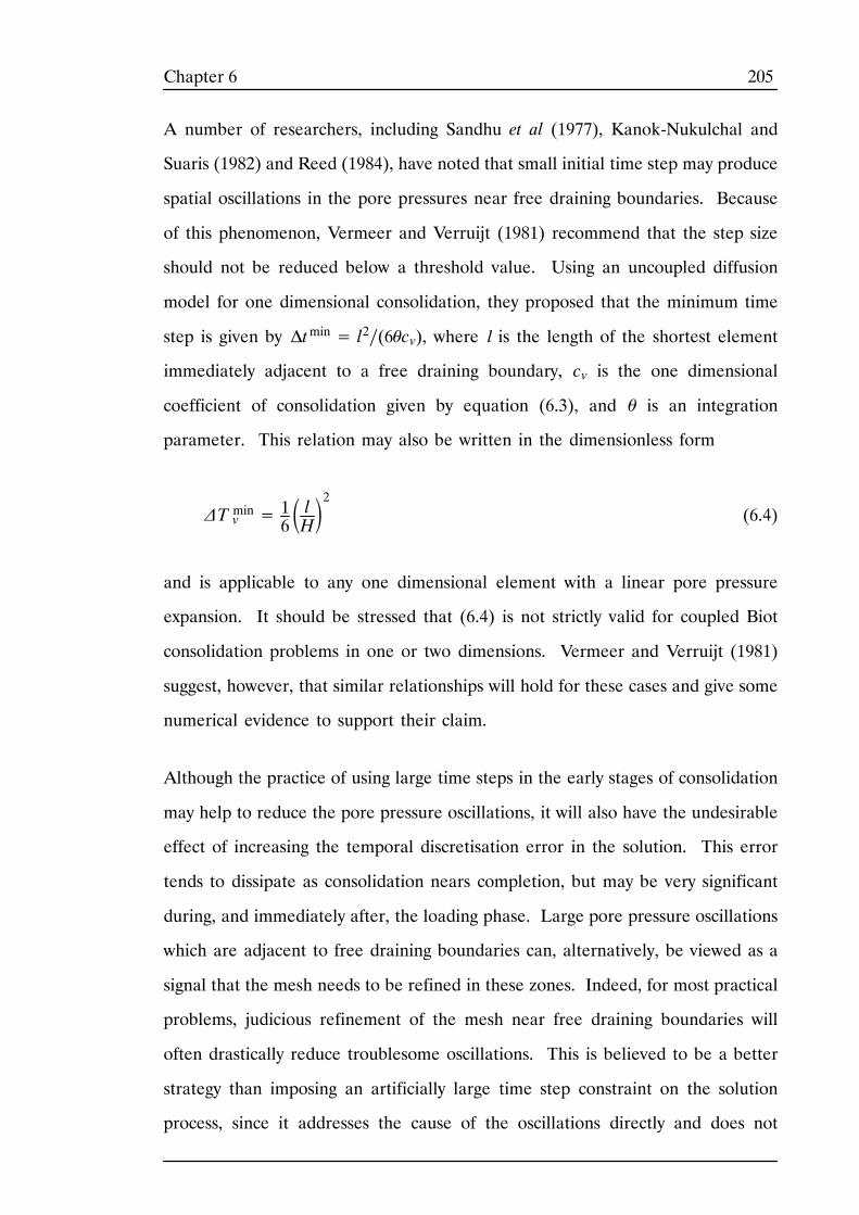
205Chapter 6
A number of researchers, including Sandhu et al (1977), Kanok-Nukulchal and
Suaris (1982) and Reed (1984), have noted that small initial time step may produce
spatial oscillations in the pore pressures near free draining boundaries. Because
of this phenomenon, Vermeer and Verruijt (1981) recommend that the step size
should not be reduced below a threshold value. Using an uncoupled diffusion
model for one dimensional consolidation, they proposed that the minimum time
step is given by Δtmin= l2∕(6θcv), where l is the length of the shortest element
immediately adjacent to a free draining boundary, cv is the one dimensional
coefficient of consolidation given by equation (6.3), and θ is an integration
parameter. This relation may also be written in the dimensionless form
ΔT minv = 16 lH2 (6.4)
and is applicable to any one dimensional element with a linear pore pressure
expansion. It should be stressed that (6.4) is not strictly valid for coupled Biot
consolidation problems in one or two dimensions. Vermeer and Verruijt (1981)
suggest, however, that similar relationships will hold for these cases and give some
numerical evidence to support their claim.
Although the practice of using large time steps in the early stages of consolidation
may help to reduce the pore pressure oscillations, it will also have the undesirable
effect of increasing the temporal discretisation error in the solution. This error
tends to dissipate as consolidation nears completion, but may be very significant
during, and immediately after, the loading phase. Large pore pressure oscillations
which are adjacent to free draining boundaries can, alternatively, be viewed as a
signal that the mesh needs to be refined in these zones. Indeed, for most practical
problems, judicious refinement of the mesh near free draining boundaries will
often drastically reduce troublesome oscillations. This is believed to be a better
strategy than imposing an artificially large time step constraint on the solution
process, since it addresses the cause of the oscillations directly and does not
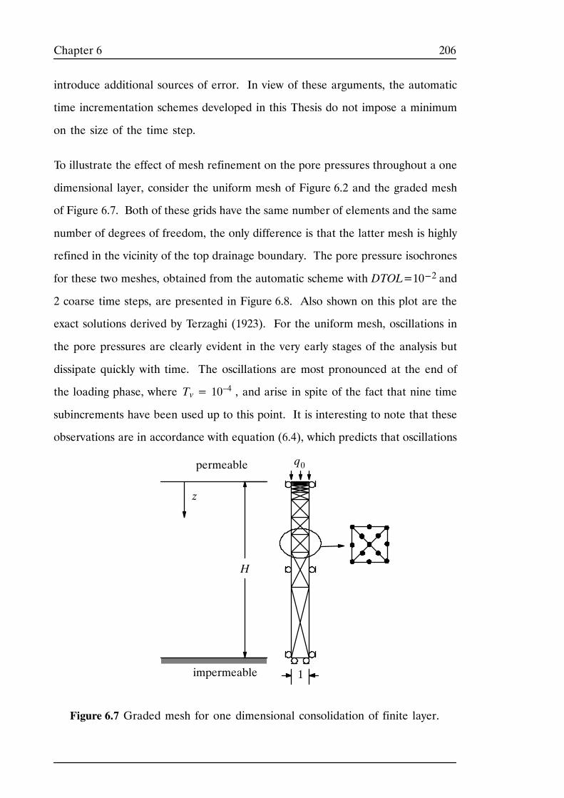
206Chapter 6
introduce additional sources of error. In view of these arguments, the automatic
time incrementation schemes developed in this Thesis do not impose a minimum
on the size of the time step.
To illustrate the effect of mesh refinement on the pore pressures throughout a one
dimensional layer, consider the uniform mesh of Figure 6.2 and the graded mesh
of Figure 6.7. Both of these grids have the same number of elements and the same
number of degrees of freedom, the only difference is that the latter mesh is highly
refined in the vicinity of the top drainage boundary. The pore pressure isochrones
for these two meshes, obtained from the automatic scheme with DTOL=10---2 and
2 coarse time steps, are presented in Figure 6.8. Also shown on this plot are the
exact solutions derived by Terzaghi (1923). For the uniform mesh, oscillations in
the pore pressures are clearly evident in the very early stages of the analysis but
dissipate quickly with time. The oscillations are most pronounced at the end of
the loading phase, where Tv= 10–4 , and arise in spite of the fact that nine time
subincrements have been used up to this point. It is interesting to note that these
observations are in accordance with equation (6.4), which predicts that oscillations
H
1
Figure 6.7 Graded mesh for one dimensional consolidation of finite layer.
impermeable
permeable
z
q0
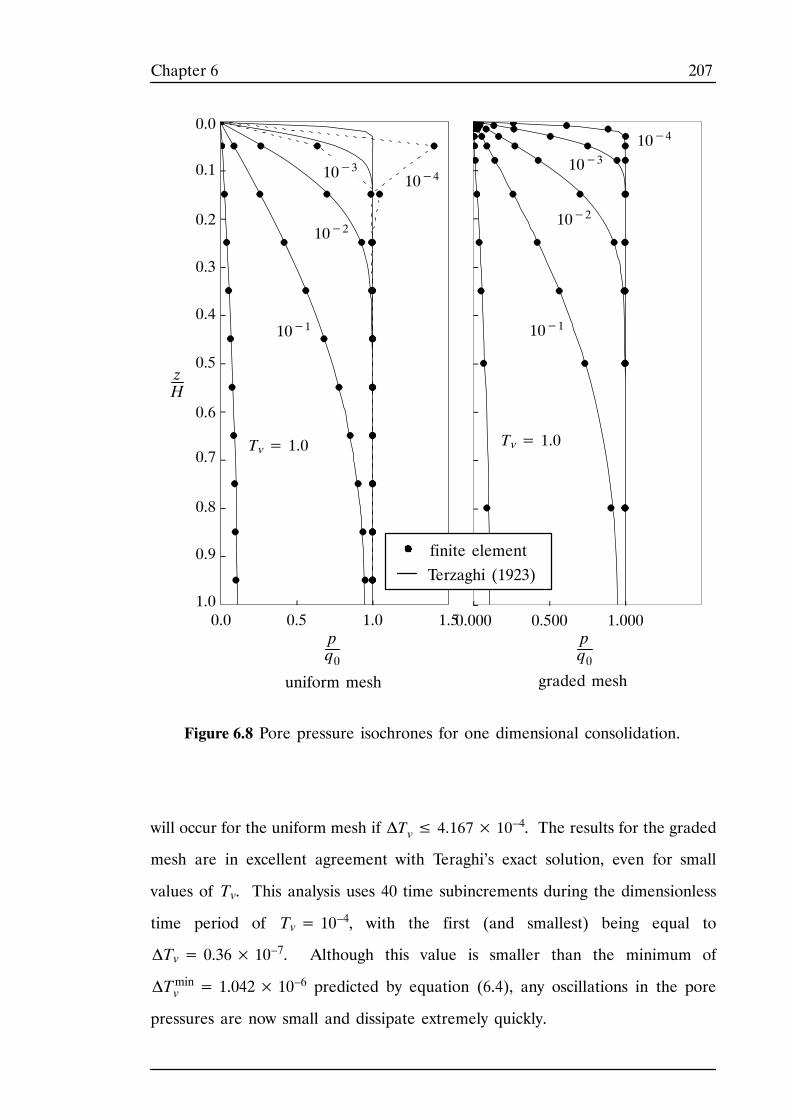
207Chapter 6
0.0 0.5 1.0 1.50.000 0.500 1.000
zH
pq0
Tv= 1.0
10−1
10−4
10−2
10−3
Figure 6.8 Pore pressure isochrones for one dimensional consolidation.
graded mesh
pq0
Tv= 1.0
10−1
10−4
10−2
uniform mesh
1.0
0.9
0.8
0.7
0.6
0.5
0.4
0.3
0.2
0.1
0.0
finite elementTerzaghi (1923)
10−3
will occur for the uniform mesh if ΔTv≤ 4.167× 10⁻⁴. The results for the graded
mesh are in excellent agreement with Teraghi’s exact solution, even for small
values of Tv. This analysis uses 40 time subincrements during the dimensionless
time period of Tv= 10–4, with the first (and smallest) being equal to
ΔTv= 0.36× 10⁻⁷. Although this value is smaller than the minimum of
ΔTminv = 1.042× 10⁻⁶ predicted by equation (6.4), any oscillations in the pore
pressures are now small and dissipate extremely quickly.
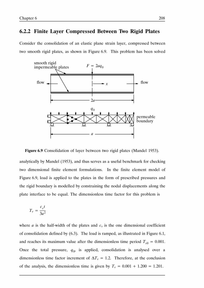
208Chapter 6
6.2.2 Finite Layer Compressed Between Two Rigid Plates
Consider the consolidation of an elastic plane strain layer, compressed between
two smooth rigid plates, as shown in Figure 6.9. This problem has been solved
smooth rigidF= 2aq0impermeable plates
2a
flowflow
Figure 6.9 Consolidation of layer between two rigid plates (Mandel 1953).
a
permeableboundary
x
q0
analytically by Mandel (1953), and thus serves as a useful benchmark for checking
two dimensional finite element formulations. In the finite element model of
Figure 6.9, load is applied to the plates in the form of prescribed pressures and
the rigid boundary is modelled by constraining the nodal displacements along the
plate interface to be equal. The dimensionless time factor for this problem is
Tv=cvt
3a2
where a is the half-width of the plates and cv is the one dimensional coefficient
of consolidation defined by (6.3). The load is ramped, as illustrated in Figure 6.1,
and reaches its maximum value after the dimensionless time period Tv0= 0.001.
Once the total pressure, q0, is applied, consolidation is analysed over a
dimensionless time factor increment of ΔTv= 1.2. Therefore, at the conclusion
of the analysis, the dimensionless time is given by Tv= 0.001+ 1.200= 1.201.
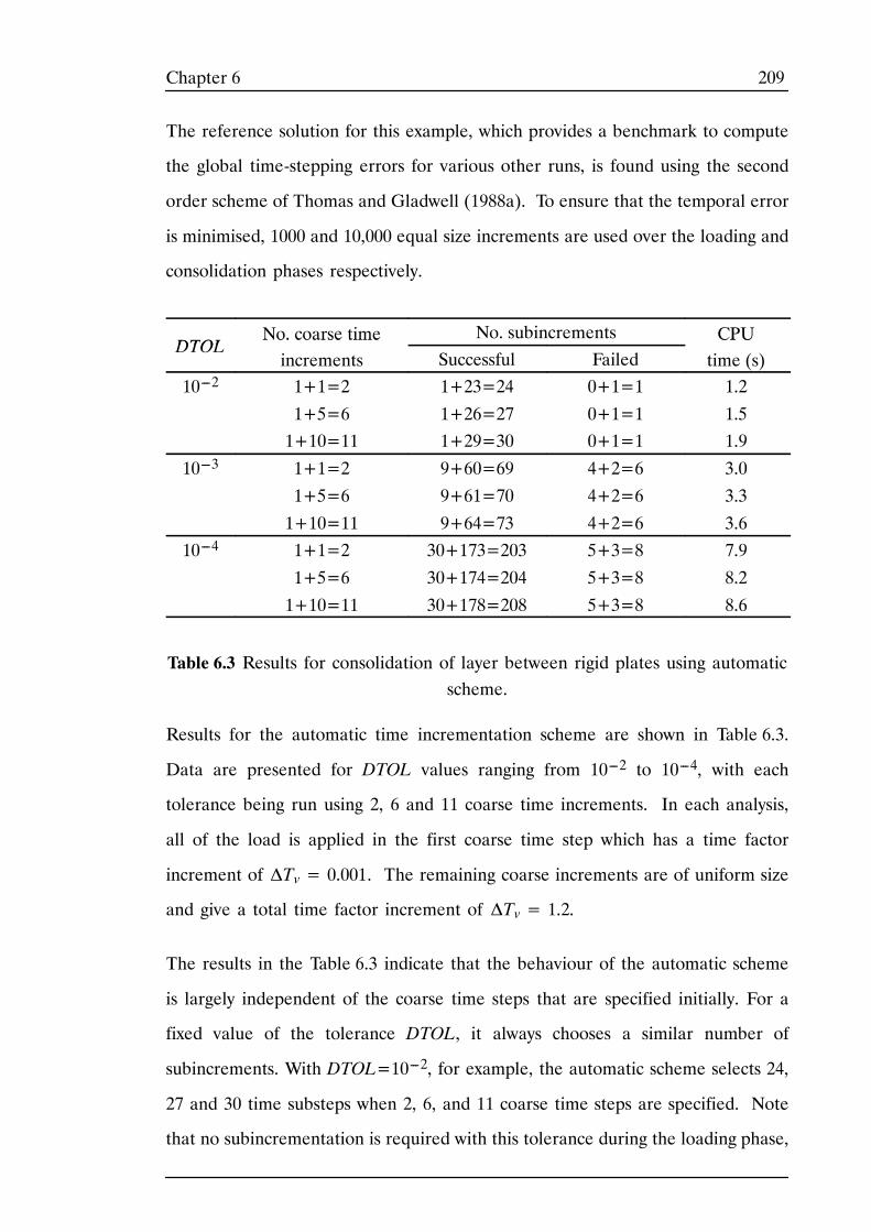
209Chapter 6
The reference solution for this example, which provides a benchmark to compute
the global time-stepping errors for various other runs, is found using the second
order scheme of Thomas and Gladwell (1988a). To ensure that the temporal error
is minimised, 1000 and 10,000 equal size increments are used over the loading and
consolidation phases respectively.
DTOLNo. coarse time No. subincrements CPU
DTOLNo. coarse timeincrements Successful Failed
CPUtime (s)
10---2 1+1=2 1+23=24 0+1=1 1.2
1+5=6 1+26=27 0+1=1 1.51+10=11 1+29=30 0+1=1 1.9
10---3 1+1=2 9+60=69 4+2=6 3.0
1+5=6 9+61=70 4+2=6 3.3
1+10=11 9+64=73 4+2=6 3.610---4 1+1=2 30+173=203 5+3=8 7.9
1+5=6 30+174=204 5+3=8 8.2
1+10=11 30+178=208 5+3=8 8.6
Table 6.3 Results for consolidation of layer between rigid plates using automaticscheme.
Results for the automatic time incrementation scheme are shown in Table 6.3.
Data are presented for DTOL values ranging from 10---2 to 10---4, with each
tolerance being run using 2, 6 and 11 coarse time increments. In each analysis,
all of the load is applied in the first coarse time step which has a time factor
increment of ΔTv= 0.001. The remaining coarse increments are of uniform size
and give a total time factor increment of ΔTv= 1.2.
The results in the Table 6.3 indicate that the behaviour of the automatic scheme
is largely independent of the coarse time steps that are specified initially. For a
fixed value of the tolerance DTOL, it always chooses a similar number of
subincrements. With DTOL=10---2, for example, the automatic scheme selects 24,
27 and 30 time substeps when 2, 6, and 11 coarse time steps are specified. Note
that no subincrementation is required with this tolerance during the loading phase,
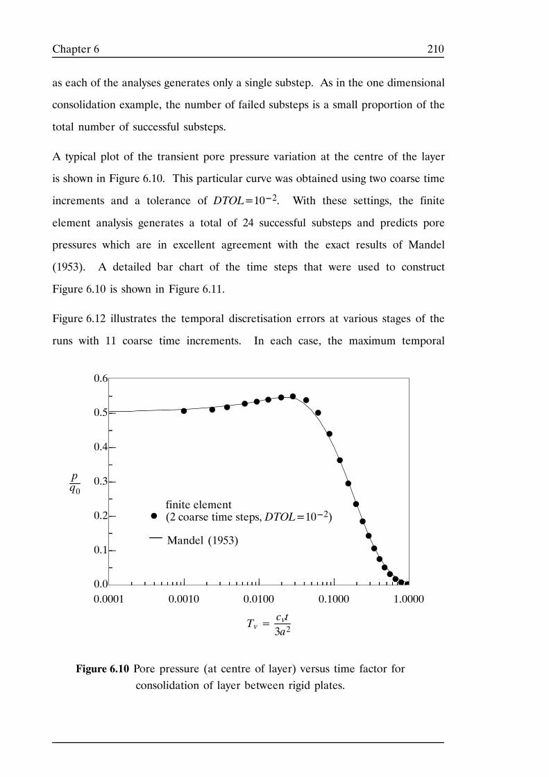
210Chapter 6
as each of the analyses generates only a single substep. As in the one dimensional
consolidation example, the number of failed substeps is a small proportion of the
total number of successful substeps.
A typical plot of the transient pore pressure variation at the centre of the layer
is shown in Figure 6.10. This particular curve was obtained using two coarse time
increments and a tolerance of DTOL=10---2. With these settings, the finite
element analysis generates a total of 24 successful substeps and predicts pore
pressures which are in excellent agreement with the exact results of Mandel
(1953). A detailed bar chart of the time steps that were used to construct
Figure 6.10 is shown in Figure 6.11.
Figure 6.12 illustrates the temporal discretisation errors at various stages of the
runs with 11 coarse time increments. In each case, the maximum temporal
0.0
0.1
0.2
0.3
0.4
0.5
0.6
0.0001 0.0010 0.0100 0.1000 1.0000
Figure 6.10 Pore pressure (at centre of layer) versus time factor forconsolidation of layer between rigid plates.
pq0
Tv=cvt3a2
Mandel (1953)
finite element(2 coarse time steps, DTOL=10---2)
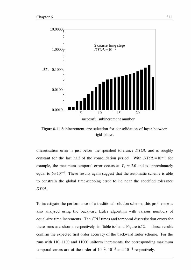
211Chapter 6
Figure 6.11 Subincrement size selection for consolidation of layer betweenrigid plates.
0.0010
0.0100
0.1000
1.0000
10.0000
5 10 15 20
ΔTv
successful subincrement number
2 coarse time stepsDTOL=10---2
discretisation error is just below the specified tolerance DTOL and is roughly
constant for the last half of the consolidation period. With DTOL=10---3, for
example, the maximum temporal error occurs at Tv≈ 2.0 and is approximately
equal to 6¢10---4. These results again suggest that the automatic scheme is able
to constrain the global time-stepping error to lie near the specified tolerance
DTOL.
To investigate the performance of a traditional solution scheme, this problem was
also analysed using the backward Euler algorithm with various numbers of
equal-size time increments. The CPU times and temporal discretisation errors for
these runs are shown, respectively, in Table 6.4 and Figure 6.12. These results
confirm the expected first order accuracy of the backward Euler scheme. For the
runs with 110, 1100 and 11000 uniform increments, the corresponding maximum
temporal errors are of the order of 10---2, 10---3 and 10---4 respectively.
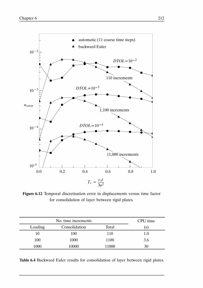
212Chapter 6
DTOL=10---2
Figure 6.12 Temporal discretisation error in displacements versus time factorfor consolidation of layer between rigid plates.
1,100 increments
110 increments
automatic (11 coarse time steps)
backward Euler
DTOL=10---3
Tv=cvt3a2
10−2
10−3
10−4 DTOL=10---4
11,000 increments
0.0 0.2 0.4 0.6 0.8 1.0
uerror
10–5
No. time increments CPU timeLoading Consolidation Total (s)
10 100 110 1.0
100 1000 1100 3.6
1000 10000 11000 30
Table 6.4 Backward Euler results for consolidation of layer between rigid plates.
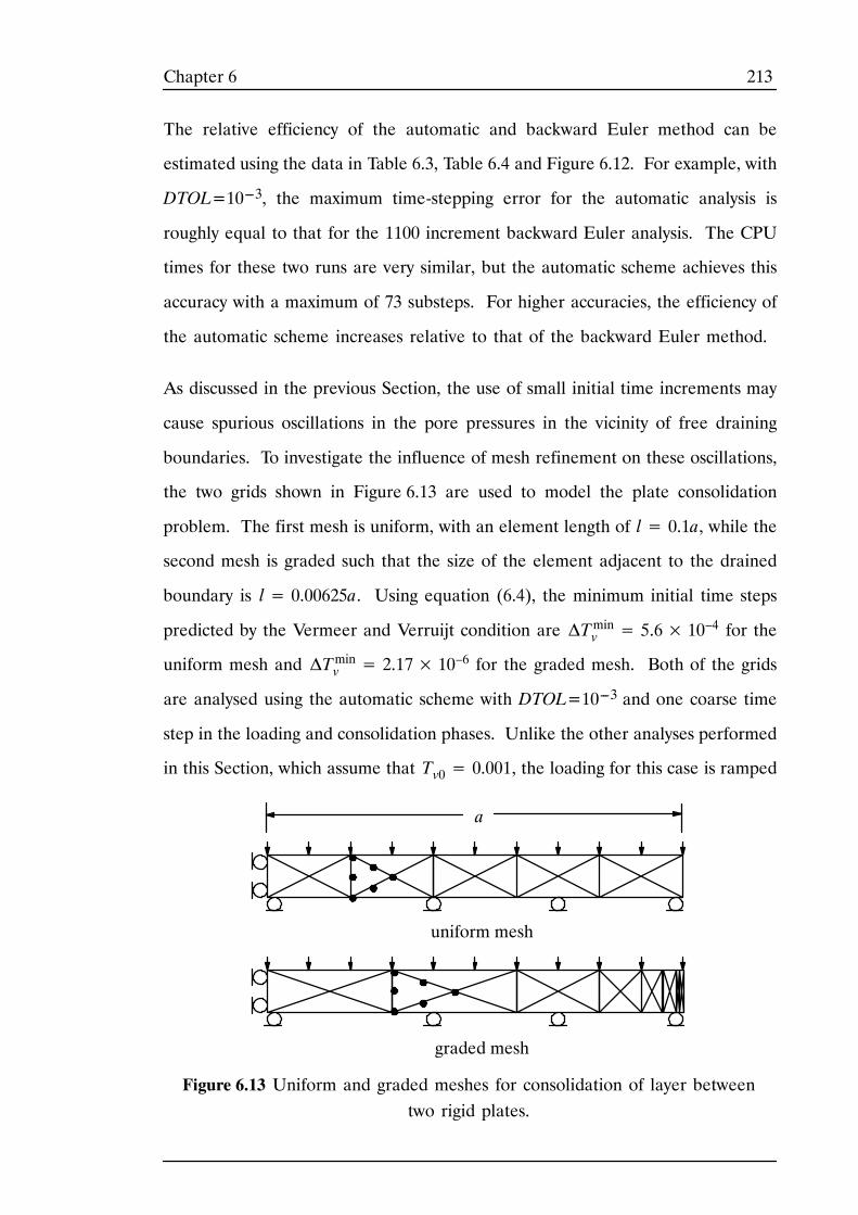
213Chapter 6
The relative efficiency of the automatic and backward Euler method can be
estimated using the data in Table 6.3, Table 6.4 and Figure 6.12. For example, with
DTOL=10---3, the maximum time-stepping error for the automatic analysis is
roughly equal to that for the 1100 increment backward Euler analysis. The CPU
times for these two runs are very similar, but the automatic scheme achieves this
accuracy with a maximum of 73 substeps. For higher accuracies, the efficiency of
the automatic scheme increases relative to that of the backward Euler method.
As discussed in the previous Section, the use of small initial time increments may
cause spurious oscillations in the pore pressures in the vicinity of free draining
boundaries. To investigate the influence of mesh refinement on these oscillations,
the two grids shown in Figure 6.13 are used to model the plate consolidation
problem. The first mesh is uniform, with an element length of l= 0.1a, while the
second mesh is graded such that the size of the element adjacent to the drained
boundary is l= 0.00625a. Using equation (6.4), the minimum initial time steps
predicted by the Vermeer and Verruijt condition are ΔTminv = 5.6× 10⁻⁴ for the
uniform mesh and ΔTminv = 2.17× 10⁻⁶ for the graded mesh. Both of the grids
are analysed using the automatic scheme with DTOL=10---3 and one coarse time
step in the loading and consolidation phases. Unlike the other analyses performed
in this Section, which assume that Tv0= 0.001, the loading for this case is ramped
Figure 6.13 Uniform and graded meshes for consolidation of layer betweentwo rigid plates.
uniform mesh
a
graded mesh
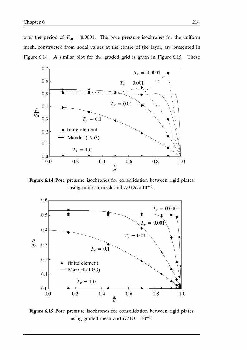
214Chapter 6
over the period of Tv0= 0.0001. The pore pressure isochrones for the uniform
mesh, constructed from nodal values at the centre of the layer, are presented in
Figure 6.14. A similar plot for the graded grid is given in Figure 6.15. These
xa
pq0
Tv= 1.0
Tv= 0.1
Tv= 0.0001
Tv= 0.01
Tv= 0.001
Figure 6.14 Pore pressure isochrones for consolidation between rigid platesusing uniform mesh and DTOL=10---3.
0.6
0.4
0.2
0.00.0 0.2 0.4 0.6 0.8 1.0
0.7
0.5
0.3
0.1
finite element
Mandel (1953)
xa
pq0
Tv= 1.0
Tv= 0.1
Tv= 0.0001
Tv= 0.01
Tv= 0.001
Figure 6.15 Pore pressure isochrones for consolidation between rigid platesusing graded mesh and DTOL=10---3.
0.6
0.4
0.2
0.00.0 0.2 0.4 0.6 0.8 1.0
0.5
0.3
0.1
finite elementMandel (1953)
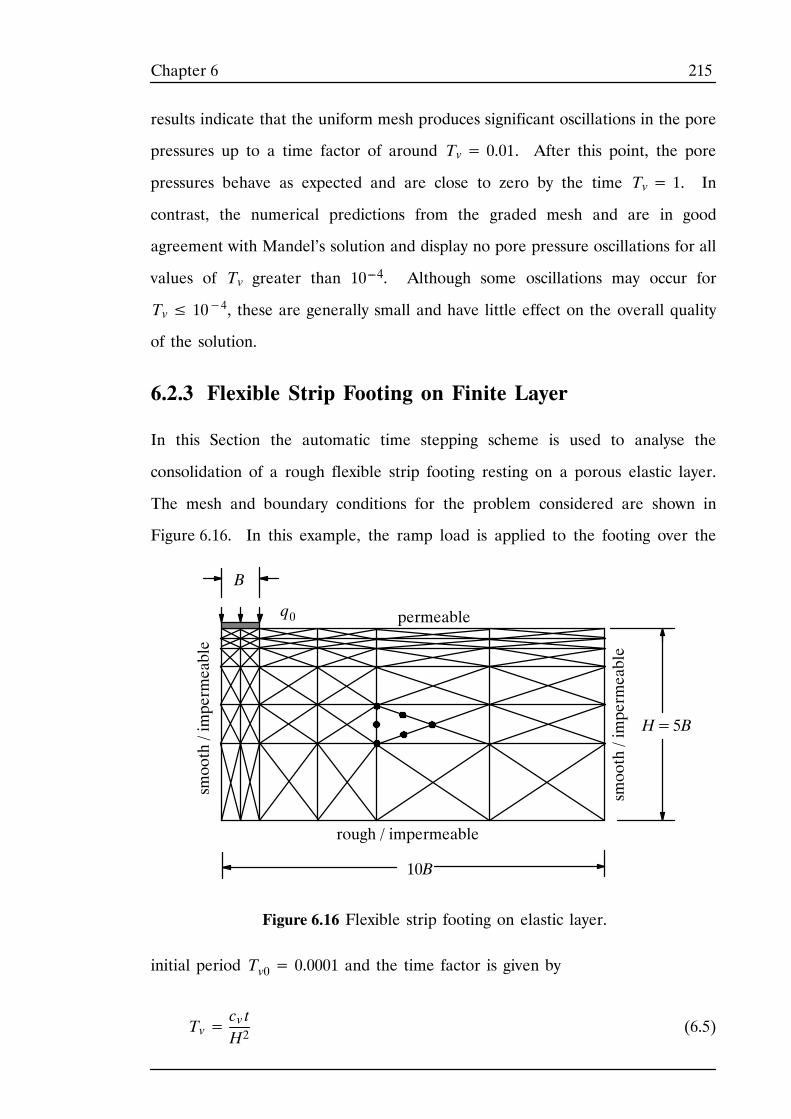
215Chapter 6
results indicate that the uniform mesh produces significant oscillations in the pore
pressures up to a time factor of around Tv= 0.01. After this point, the pore
pressures behave as expected and are close to zero by the time Tv= 1. In
contrast, the numerical predictions from the graded mesh and are in good
agreement with Mandel’s solution and display no pore pressure oscillations for all
values of Tv greater than 10---4. Although some oscillations may occur for
Tv≤ 10−4, these are generally small and have little effect on the overall quality
of the solution.
6.2.3 Flexible Strip Footing on Finite Layer
In this Section the automatic time stepping scheme is used to analyse the
consolidation of a rough flexible strip footing resting on a porous elastic layer.
The mesh and boundary conditions for the problem considered are shown in
Figure 6.16. In this example, the ramp load is applied to the footing over the
smooth/impermeable
smooth/impermeable
rough / impermeable
permeable
10B
H=5B
B
Figure 6.16 Flexible strip footing on elastic layer.
q0
initial period Tv0= 0.0001 and the time factor is given by
Tv=cv tH2
(6.5)
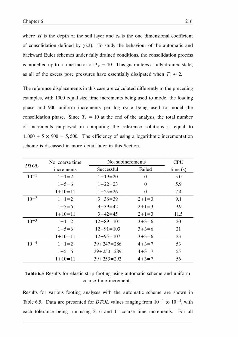
216Chapter 6
where H is the depth of the soil layer and cv is the one dimensional coefficient
of consolidation defined by (6.3). To study the behaviour of the automatic and
backward Euler schemes under fully drained conditions, the consolidation process
is modelled up to a time factor of Tv= 10. This guarantees a fully drained state,
as all of the excess pore pressures have essentially dissipated when Tv≈ 2.
The reference displacements in this case are calculated differently to the preceding
examples, with 1000 equal size time increments being used to model the loading
phase and 900 uniform increments per log cycle being used to model the
consolidation phase. Since Tv= 10 at the end of the analysis, the total number
of increments employed in computing the reference solutions is equal to
1, 000+ 5× 900= 5, 500. The efficiency of using a logarithmic incrementation
scheme is discussed in more detail later in this Section.
DTOLNo. coarse time No. subincrements CPU
DTOLo. coa se t eincrements Successful Failed
C Utime (s)
10---1 1+1=2 1+19=20 0 5.0
1+5=6 1+22=23 0 5.9
1+10=11 1+25=26 0 7.410---2 1+1=2 3+36=39 2+1=3 9.1
1+5=6 3+39=42 2+1=3 9.9
1+10=11 3+42=45 2+1=3 11.510---3 1+1=2 12+89=101 3+3=6 20
1+5=6 12+91=103 3+3=6 21
1+10=11 12+95=107 3+3=6 23
10---4 1+1=2 39+247=286 4+3=7 531+5=6 39+250=289 4+3=7 55
1+10=11 39+253=292 4+3=7 56
Table 6.5 Results for elastic strip footing using automatic scheme and uniformcoarse time increments.
Results for various footing analyses with the automatic scheme are shown in
Table 6.5. Data are presented for DTOL values ranging from 10---1 to 10---4, with
each tolerance being run using 2, 6 and 11 coarse time increments. For all
217Chapter 6
analyses, the load is applied in the first coarse time step which has a time factor
increment of ΔTv0= 0.0001. The remaining coarse increments are of near
uniform size and advance the solution to Tv= 10. As in previous examples, these
results indicate that the automatic scheme chooses a similar number of substeps
for each value of DTOL, regardless of the initial coarse time step size. With
DTOL=10---2, for example, the new algorithm generates 39, 42 and 45 substeps
for runs with 2, 6 and 11 initial coarse time steps. The bulk of these substeps occur
in the consolidation phase, with only three substeps being generated during the
application of the load.
To illustrate the accuracy of the automatic scheme, Figure 6.17 shows two plots of
the degree of consolidation at the centre of the footing versus the time factor.
These results were generated using two coarse time steps and DTOL values of
10---1 and 10---2. The finite element predictions for both of these tolerances are
very similar and match the analytic solution of Booker (1974) over all of the
loading range. The small amount of deviation indicated is attributable to the
spatial discretisation error. It is interesting to note that, on the scale of
Figure 6.17, the results for the most stringent tolerance of DTOL=10---4 are
indistinguishable from those for DTOL=10---2 . This suggests the latter value is
a practical starting point for analysing the behaviour of elastic two dimensional
consolidation problems. To gain some insight into the step selection philosophy
of the automatic scheme, Figure 6.18 shows the successful time step sizes for the
analysis with DTOL=10---2. As in previous examples, the step size is small at the
start of the analysis and increases consistently throughout the entire consolidation
process. The step size ranges from a minimum value of ΔTv= 3× 10⁻⁵ to a
maximum of ΔTv= 3.32 and, on average, grows by an order of magnitude over
6 or 7 consecutive substeps. An alternative picture of the substep size variation,
for all values of DTOL, is shown in Figure 6.19. This plot indicates that all of the
analyses adopt a similar step size once consolidation is complete, regardless of the
value of the error tolerance. This is a direct result of the governing differential
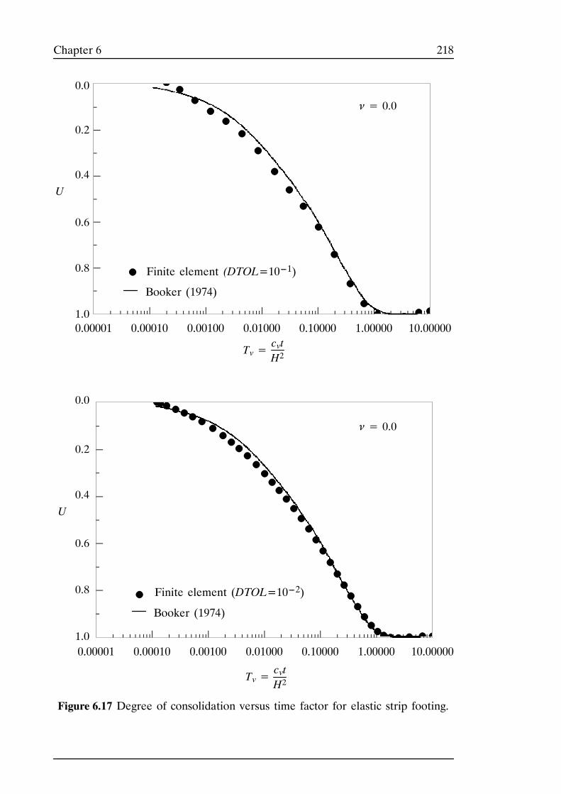
218Chapter 6
0.00001 0.00010 0.00100 0.01000 0.10000 1.00000 10.00000
0.00001 0.00010 0.00100 0.01000 0.10000 1.00000 10.00000
Figure 6.17 Degree of consolidation versus time factor for elastic strip footing.
U
Tv=cvtH2
U
Tv=cvtH2
0.0
0.2
0.4
0.6
0.8
1.0
0.0
0.2
0.4
0.6
0.8
1.0
Finite element (DTOL=10---1)
Booker (1974)
Finite element (DTOL=10---2)
Booker (1974)
ν= 0.0
ν= 0.0
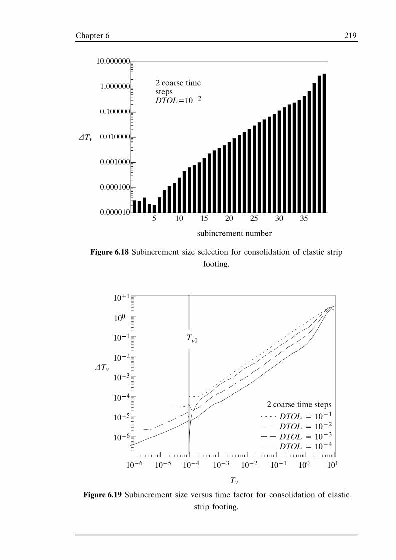
219Chapter 6
Figure 6.18 Subincrement size selection for consolidation of elastic stripfooting.
0.000010
0.000100
0.001000
0.010000
0.100000
1.000000
10.000000
5 10 15 20 25 30 35
ΔTv
subincrement number
2 coarse timestepsDTOL=10---2
Figure 6.19 Subincrement size versus time factor for consolidation of elasticstrip footing.
Tv0
Tv
DTOL= 10−4DTOL= 10−3DTOL= 10−2DTOL= 10−1
10010---110---210---4 10---310---510---6
10---1
10---2
10---3
10---4
10---5
10---6
100
10+1
101
ΔTv
2 coarse time steps
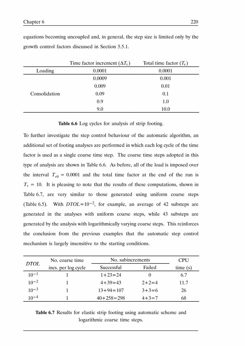
220Chapter 6
equations becoming uncoupled and, in general, the step size is limited only by the
growth control factors discussed in Section 5.5.1.
Time factor increment (ΔTv) Total time factor (Tv)
Loading 0.0001 0.00010.0009 0.001
0.009 0.01
Consolidation 0.09 0.1
0.9 1.09.0 10.0
Table 6.6 Log cycles for analysis of strip footing.
To further investigate the step control behaviour of the automatic algorithm, an
additional set of footing analyses are performed in which each log cycle of the time
factor is used as a single coarse time step. The coarse time steps adopted in this
type of analysis are shown in Table 6.6. As before, all of the load is imposed over
the interval Tv0= 0.0001 and the total time factor at the end of the run is
Tv= 10. It is pleasing to note that the results of these computations, shown in
Table 6.7, are very similar to those generated using uniform coarse steps
(Table 6.5). With DTOL=10---2, for example, an average of 42 substeps are
generated in the analyses with uniform coarse steps, while 43 substeps are
generated by the analysis with logarithmically varying coarse steps. This reinforces
the conclusion from the previous examples that the automatic step control
mechanism is largely insensitive to the starting conditions.
DTOLNo. coarse time No. subincrements CPU
DTOLo. coa se t e
incs. per log cycle Successful FailedC Utime (s)
10---1 1 1+23=24 0 6.7
10---2 1 4+39=43 2+2=4 11.7
10---3 1 13+94=107 3+3=6 26
10---4 1 40+258=298 4+3=7 68
Table 6.7 Results for elastic strip footing using automatic scheme andlogarithmic coarse time steps.
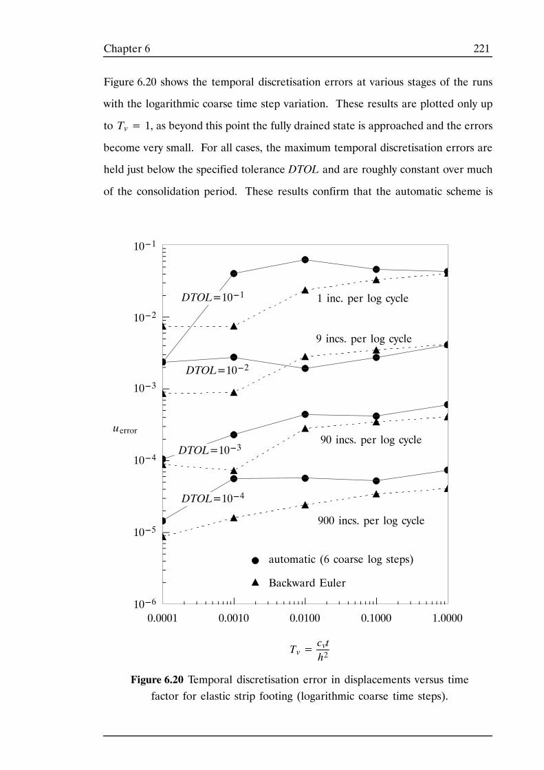
221Chapter 6
Figure 6.20 shows the temporal discretisation errors at various stages of the runs
with the logarithmic coarse time step variation. These results are plotted only up
to Tv= 1, as beyond this point the fully drained state is approached and the errors
become very small. For all cases, the maximum temporal discretisation errors are
held just below the specified tolerance DTOL and are roughly constant over much
of the consolidation period. These results confirm that the automatic scheme is
0.0001 0.0010 0.0100 0.1000 1.0000
Figure 6.20 Temporal discretisation error in displacements versus timefactor for elastic strip footing (logarithmic coarse time steps).
900 incs. per log cycle
90 incs. per log cycle
9 incs. per log cycle
1 inc. per log cycle
DTOL=10---4
DTOL=10---3
DTOL=10---2
DTOL=10---1
automatic (6 coarse log steps)
Backward Euler
Tv=cvth2
10---1
10---2
10---3
10---4
10---5
10---6
uerror
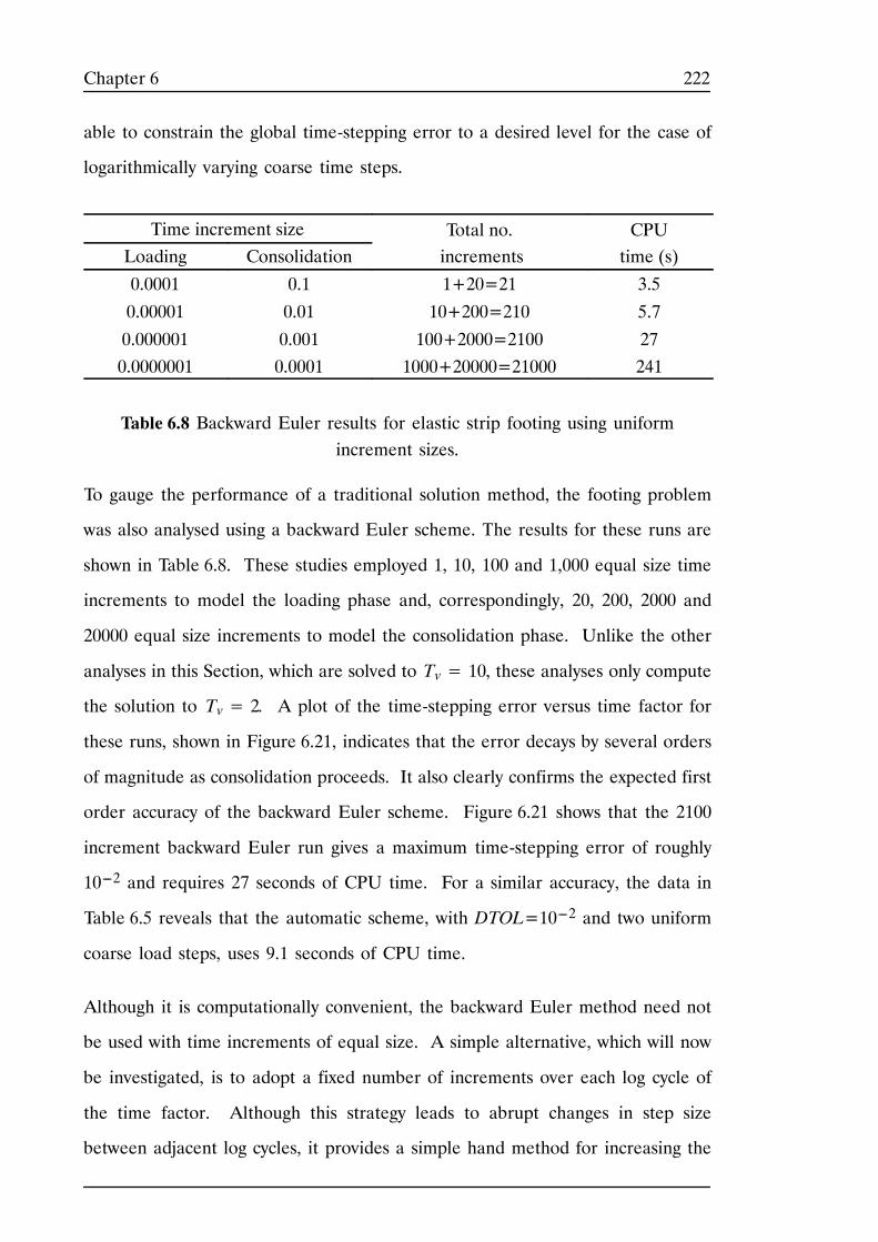
222Chapter 6
able to constrain the global time-stepping error to a desired level for the case of
logarithmically varying coarse time steps.
Time increment size Total no. CPULoading Consolidation increments time (s)
0.0001 0.1 1+20=21 3.5
0.00001 0.01 10+200=210 5.7
0.000001 0.001 100+2000=2100 270.0000001 0.0001 1000+20000=21000 241
Table 6.8 Backward Euler results for elastic strip footing using uniformincrement sizes.
To gauge the performance of a traditional solution method, the footing problem
was also analysed using a backward Euler scheme. The results for these runs are
shown in Table 6.8. These studies employed 1, 10, 100 and 1,000 equal size time
increments to model the loading phase and, correspondingly, 20, 200, 2000 and
20000 equal size increments to model the consolidation phase. Unlike the other
analyses in this Section, which are solved to Tv= 10, these analyses only compute
the solution to Tv= 2. A plot of the time-stepping error versus time factor for
these runs, shown in Figure 6.21, indicates that the error decays by several orders
of magnitude as consolidation proceeds. It also clearly confirms the expected first
order accuracy of the backward Euler scheme. Figure 6.21 shows that the 2100
increment backward Euler run gives a maximum time-stepping error of roughly
10---2 and requires 27 seconds of CPU time. For a similar accuracy, the data in
Table 6.5 reveals that the automatic scheme, with DTOL=10---2 and two uniform
coarse load steps, uses 9.1 seconds of CPU time.
Although it is computationally convenient, the backward Euler method need not
be used with time increments of equal size. A simple alternative, which will now
be investigated, is to adopt a fixed number of increments over each log cycle of
the time factor. Although this strategy leads to abrupt changes in step size
between adjacent log cycles, it provides a simple hand method for increasing the
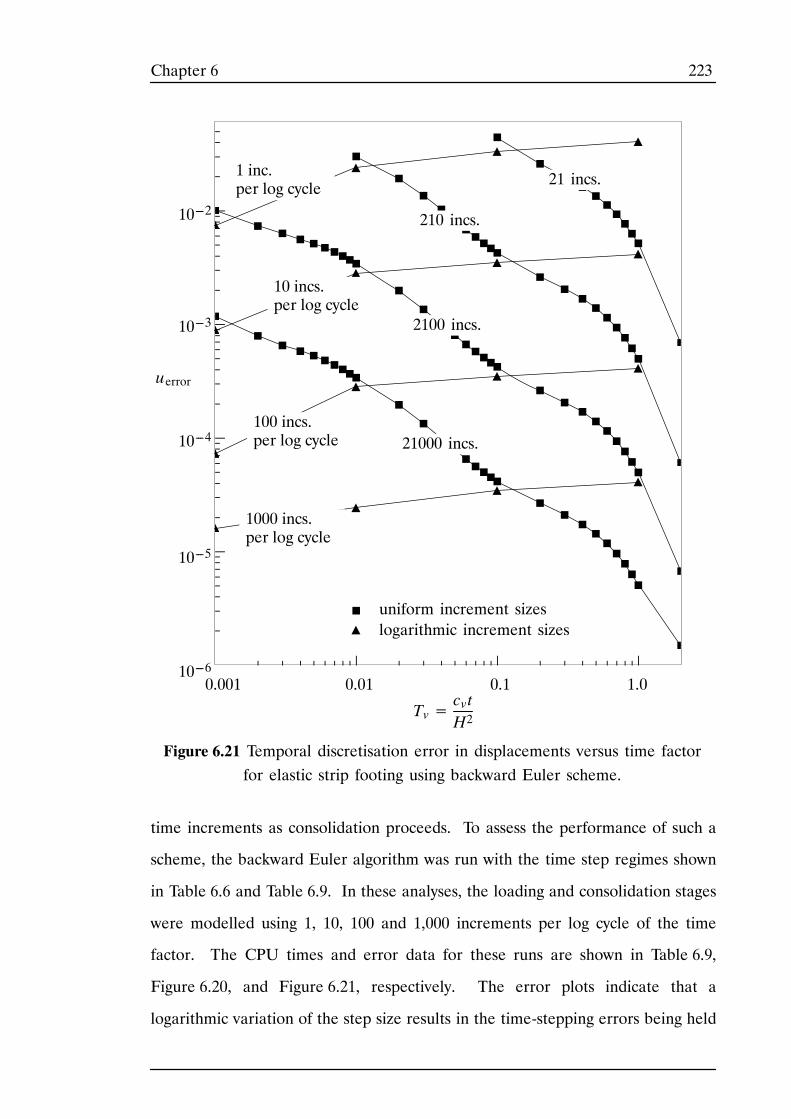
223Chapter 6
Figure 6.21 Temporal discretisation error in displacements versus time factorfor elastic strip footing using backward Euler scheme.
1000 incs.per log cycle
logarithmic increment sizesuniform increment sizes
1 inc.per log cycle
Tv=cvtH2
10---2
10---3
10---4
10---5
10---61.00.001 0.01 0.1
10 incs.per log cycle
100 incs.per log cycle
21 incs.
210 incs.
2100 incs.
21000 incs.
uerror
time increments as consolidation proceeds. To assess the performance of such a
scheme, the backward Euler algorithm was run with the time step regimes shown
in Table 6.6 and Table 6.9. In these analyses, the loading and consolidation stages
were modelled using 1, 10, 100 and 1,000 increments per log cycle of the time
factor. The CPU times and error data for these runs are shown in Table 6.9,
Figure 6.20, and Figure 6.21, respectively. The error plots indicate that a
logarithmic variation of the step size results in the time-stepping errors being held
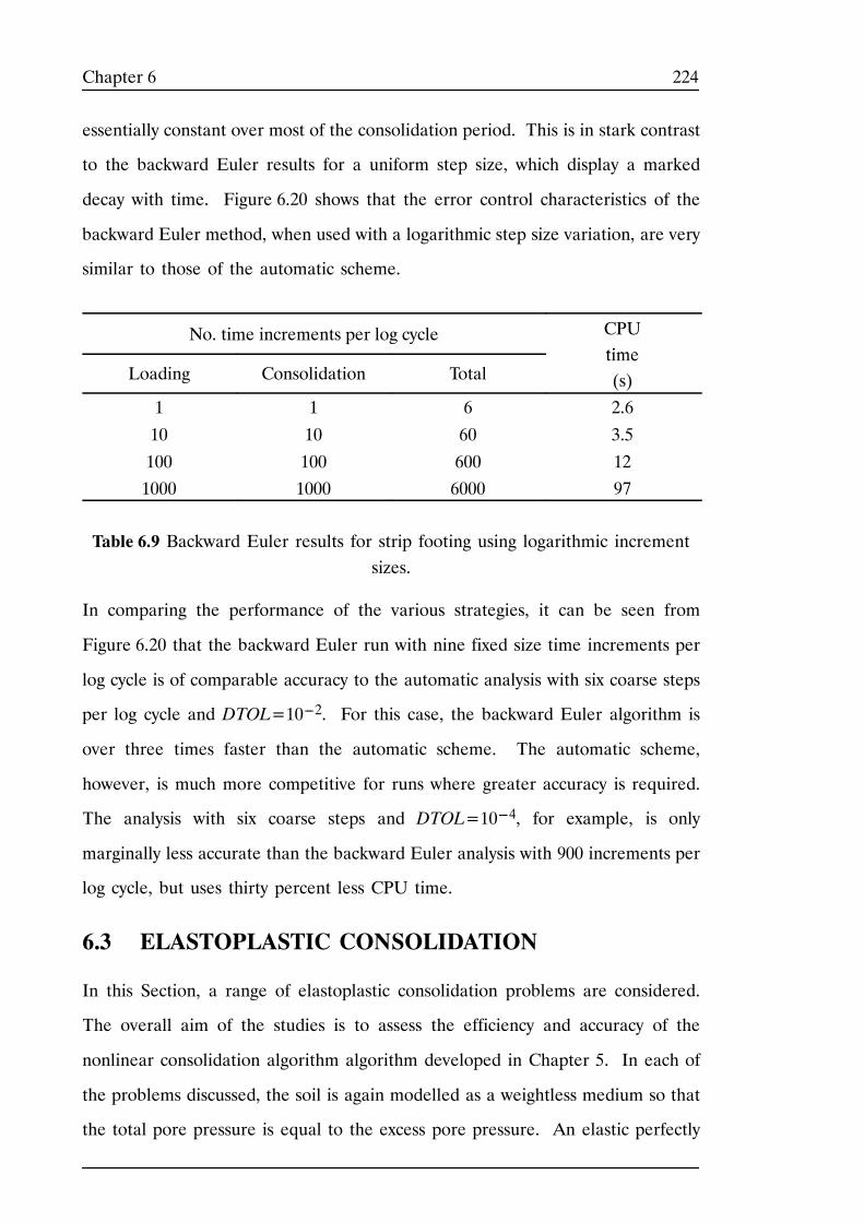
224Chapter 6
essentially constant over most of the consolidation period. This is in stark contrast
to the backward Euler results for a uniform step size, which display a marked
decay with time. Figure 6.20 shows that the error control characteristics of the
backward Euler method, when used with a logarithmic step size variation, are very
similar to those of the automatic scheme.
No. time increments per log cycle CPUtime
Loading Consolidation Totaltime(s)
1 1 6 2.6
10 10 60 3.5
100 100 600 121000 1000 6000 97
Table 6.9 Backward Euler results for strip footing using logarithmic incrementsizes.
In comparing the performance of the various strategies, it can be seen from
Figure 6.20 that the backward Euler run with nine fixed size time increments per
log cycle is of comparable accuracy to the automatic analysis with six coarse steps
per log cycle and DTOL=10---2. For this case, the backward Euler algorithm is
over three times faster than the automatic scheme. The automatic scheme,
however, is much more competitive for runs where greater accuracy is required.
The analysis with six coarse steps and DTOL=10---4, for example, is only
marginally less accurate than the backward Euler analysis with 900 increments per
log cycle, but uses thirty percent less CPU time.
6.3 ELASTOPLASTIC CONSOLIDATION
In this Section, a range of elastoplastic consolidation problems are considered.
The overall aim of the studies is to assess the efficiency and accuracy of the
nonlinear consolidation algorithm algorithm developed in Chapter 5. In each of
the problems discussed, the soil is again modelled as a weightless medium so that
the total pore pressure is equal to the excess pore pressure. An elastic perfectly
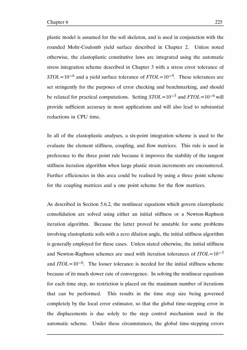
225Chapter 6
plastic model is assumed for the soil skeleton, and is used in conjunction with the
rounded Mohr-Coulomb yield surface described in Chapter 2. Unless noted
otherwise, the elastoplastic constitutive laws are integrated using the automatic
stress integration scheme described in Chapter 3 with a stress error tolerance of
STOL=10---6 and a yield surface tolerance of FTOL=10---9. These tolerances are
set stringently for the purposes of error checking and benchmarking, and should
be relaxed for practical computations. Setting STOL=10---3 and FTOL=10---6 will
provide sufficient accuracy in most applications and will also lead to substantial
reductions in CPU time.
In all of the elastoplastic analyses, a six-point integration scheme is used to the
evaluate the element stiffness, coupling, and flow matrices. This rule is used in
preference to the three point rule because it improves the stability of the tangent
stiffness iteration algorithm when large plastic strain increments are encountered.
Further efficiencies in this area could be realised by using a three point scheme
for the coupling matrices and a one point scheme for the flow matrices.
As described in Section 5.6.2, the nonlinear equations which govern elastoplastic
consolidation are solved using either an initial stiffness or a Newton-Raphson
iteration algorithm. Because the latter proved be unstable for some problems
involving elastoplastic soils with a zero dilation angle, the initial stiffness algorithm
is generally employed for these cases. Unless stated otherwise, the initial stiffness
and Newton-Raphson schemes are used with iteration tolerances of ITOL=10---3
and ITOL=10---6. The looser tolerance is needed for the initial stiffness scheme
because of its much slower rate of convergence. In solving the nonlinear equations
for each time step, no restriction is placed on the maximum number of iterations
that can be performed. This results in the time step size being governed
completely by the local error estimator, so that the global time-stepping error in
the displacements is due solely to the step control mechanism used in the
automatic scheme. Under these circumstances, the global time-stepping errors
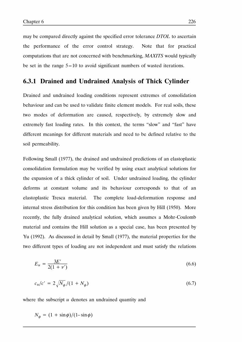
226Chapter 6
may be compared directly against the specified error tolerance DTOL to ascertain
the performance of the error control strategy. Note that for practical
computations that are not concerned with benchmarking, MAXITS would typically
be set in the range 5---10 to avoid significant numbers of wasted iterations.
6.3.1 Drained and Undrained Analysis of Thick Cylinder
Drained and undrained loading conditions represent extremes of consolidation
behaviour and can be used to validate finite element models. For real soils, these
two modes of deformation are caused, respectively, by extremely slow and
extremely fast loading rates. In this context, the terms “slow” and “fast” have
different meanings for different materials and need to be defined relative to the
soil permeability.
Following Small (1977), the drained and undrained predictions of an elastoplastic
consolidation formulation may be verified by using exact analytical solutions for
the expansion of a thick cylinder of soil. Under undrained loading, the cylinder
deforms at constant volume and its behaviour corresponds to that of an
elastoplastic Tresca material. The complete load-deformation response and
internal stress distribution for this condition has been given by Hill (1950). More
recently, the fully drained analytical solution, which assumes a Mohr-Coulomb
material and contains the Hill solution as a special case, has been presented by
Yu (1992). As discussed in detail by Small (1977), the material properties for the
two different types of loading are not independent and must satisfy the relations
Eu= 3E′2(1+ ν′) (6.6)
cu∕c′ = 2 Nφ ∕(1+Nφ) (6.7)
where the subscript u denotes an undrained quantity and
Nφ= (1+ sinφ)∕(1– sinφ)
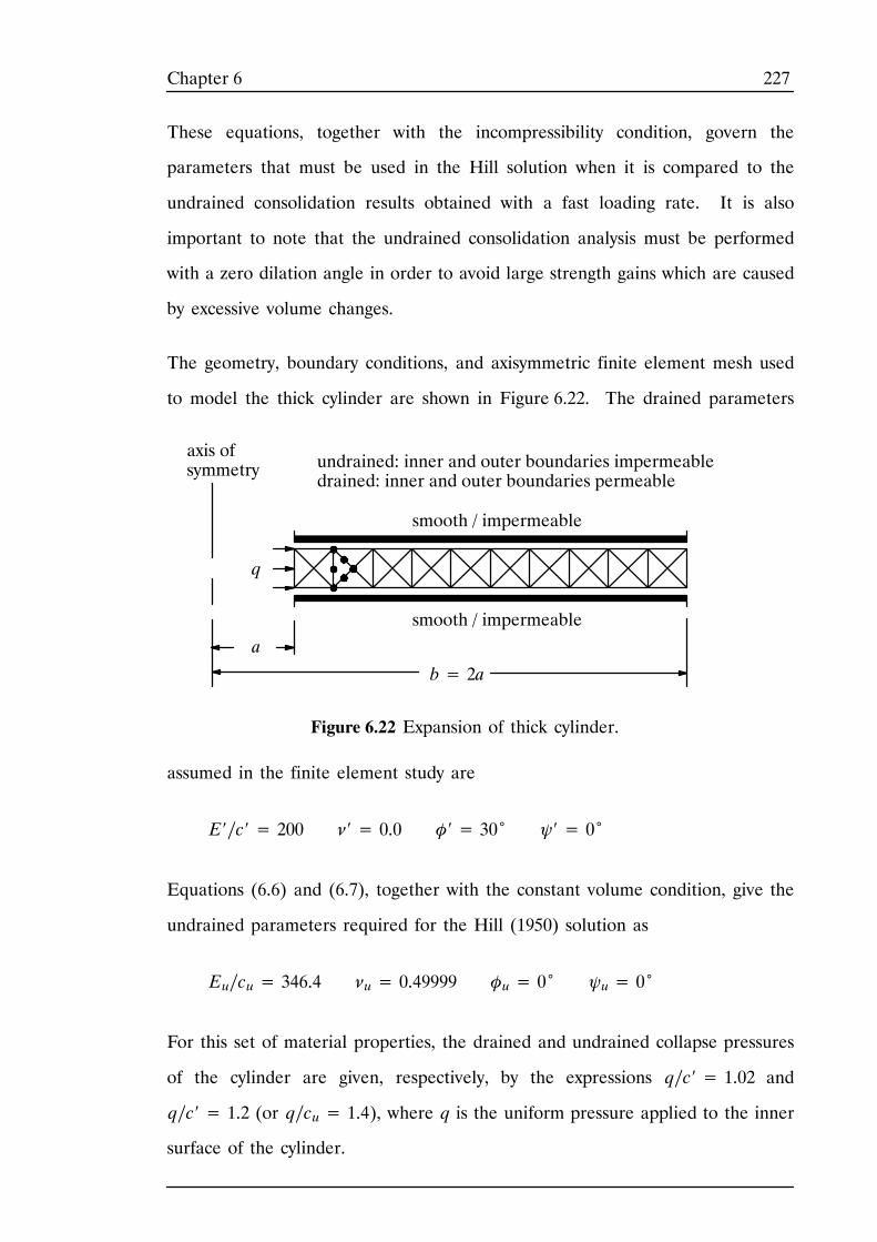
227Chapter 6
These equations, together with the incompressibility condition, govern the
parameters that must be used in the Hill solution when it is compared to the
undrained consolidation results obtained with a fast loading rate. It is also
important to note that the undrained consolidation analysis must be performed
with a zero dilation angle in order to avoid large strength gains which are caused
by excessive volume changes.
The geometry, boundary conditions, and axisymmetric finite element mesh used
to model the thick cylinder are shown in Figure 6.22. The drained parameters
smooth / impermeable
smooth / impermeable
axis ofsymmetry
Figure 6.22 Expansion of thick cylinder.
q
a
b= 2a
undrained: inner and outer boundaries impermeabledrained: inner and outer boundaries permeable
assumed in the finite element study are
E′∕c′ = 200 ν′ = 0.0 φ′ = 30˚ ψ′ = 0˚
Equations (6.6) and (6.7), together with the constant volume condition, give the
undrained parameters required for the Hill (1950) solution as
Eu∕cu= 346.4 νu= 0.49999 φu= 0˚ ψu= 0˚
For this set of material properties, the drained and undrained collapse pressures
of the cylinder are given, respectively, by the expressions q∕c′ = 1.02 and
q∕c′ = 1.2 (or q∕cu= 1.4), where q is the uniform pressure applied to the inner
surface of the cylinder.
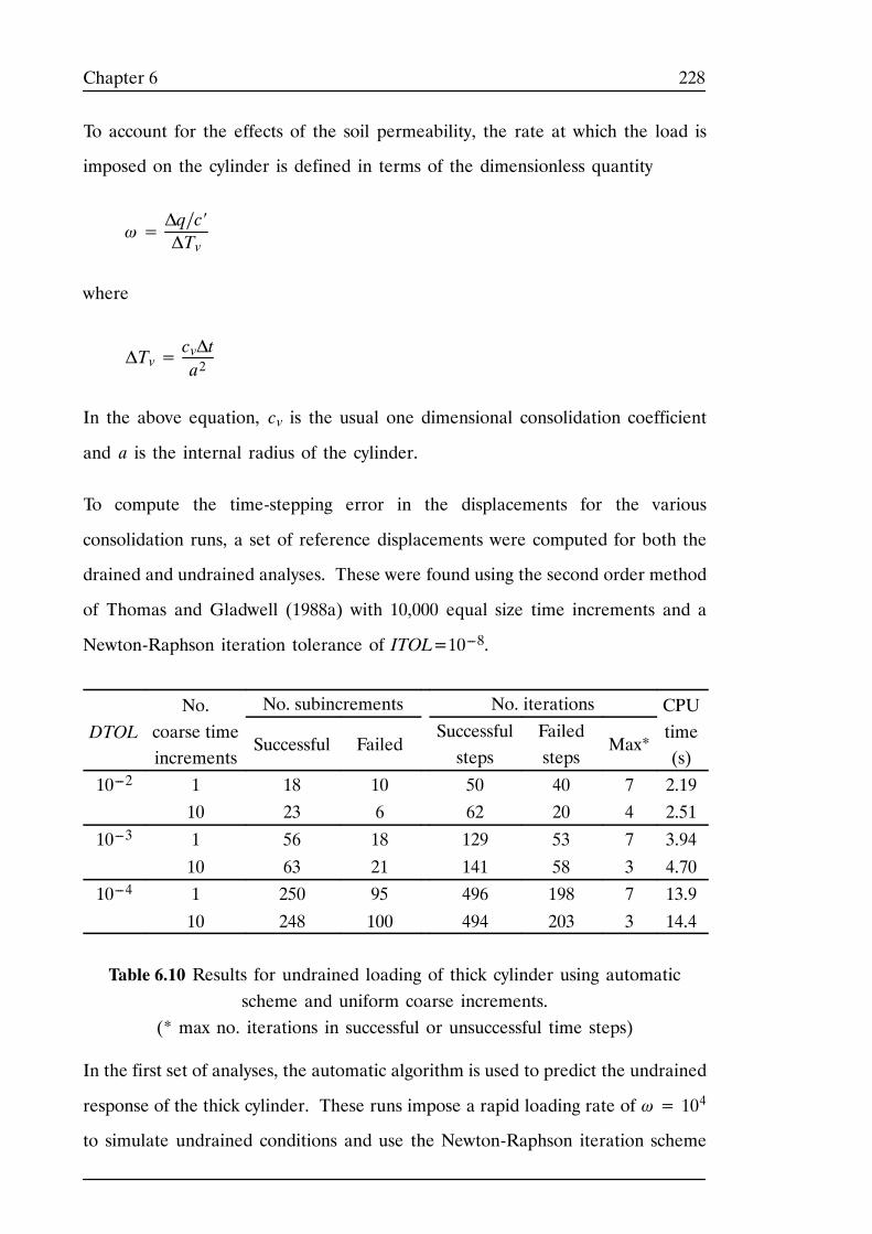
228Chapter 6
To account for the effects of the soil permeability, the rate at which the load is
imposed on the cylinder is defined in terms of the dimensionless quantity
ω=Δq∕c′ΔTv
where
ΔTv=cvΔta2
In the above equation, cv is the usual one dimensional consolidation coefficient
and a is the internal radius of the cylinder.
To compute the time-stepping error in the displacements for the various
consolidation runs, a set of reference displacements were computed for both the
drained and undrained analyses. These were found using the second order method
of Thomas and Gladwell (1988a) with 10,000 equal size time increments and a
Newton-Raphson iteration tolerance of ITOL=10---8.
No. No. subincrements No. iterations CPUDTOL
No.coarse timeincrements
Successful FailedSuccessfulsteps
Failedsteps
Max*
CPUtime(s)
10---2 1 18 10 50 40 7 2.1910 23 6 62 20 4 2.51
10---3 1 56 18 129 53 7 3.94
10 63 21 141 58 3 4.7010---4 1 250 95 496 198 7 13.9
10 248 100 494 203 3 14.4
Table 6.10 Results for undrained loading of thick cylinder using automaticscheme and uniform coarse increments.
(* max no. iterations in successful or unsuccessful time steps)
In the first set of analyses, the automatic algorithm is used to predict the undrained
response of the thick cylinder. These runs impose a rapid loading rate of ω= 104
to simulate undrained conditions and use the Newton-Raphson iteration scheme
229Chapter 6
to solve the incremental equations for each time step. As shown in Table 6.10,
results are generated for analyses using 1 and 10 coarse time steps with error
tolerances of DTOL=10---2, 10---3 and 10---4. In all cases, the automatic algorithm
selects a similar number of subincrements for analyses performed with the same
displacement tolerance. With DTOL=10---2, for example, the runs with 1 and 10
coarse time steps generate, respectively, 18 and 23 successful subincrements.
Similarly, for a tolerance of DTOL=10---3, the analyses employs 56 and 63
successful subincrements.
The relatively high number of failed subincrements for this example is a
consequence of the fact that the undrained deformation response of the cylinder
is particularly sensitive to the effects of Gauss points turning plastic. Because of
the abrupt change in behaviour that is imposed by an elastic perfectly plastic
model, an elastic-plastic transition for a single Gauss point has a pronounced affect
on the value of the local error indicator for this particular problem. This impacts
on the present scheme as consecutive substeps are allowed to double in size to
enable rapid growth of the time step during later stages of the consolidation
process. One possible strategy for reducing the number of failed substeps is to
limit this growth factor to a lower value of around ten percent, as was done in the
automatic load stepping algorithm of Chapter 4. Since most of the failed steps
will occur during application of the load, this restriction would not need to be
enforced during the consolidation phase. Other cases considered later in this
Section do not exhibit a large proportion of failed steps, so this refinement has
not been incorporated in this Thesis.
On average, only two to three iterations are required for each successful substep
of the automatic scheme. This reflects the ability of the Newton-Raphson
algorithm to provide rapid convergence when it used with an appropriate time
step. As expected, the maximum number of iterations for a given analysis is
highest for cases where the maximum load is applied in a single coarse time step.
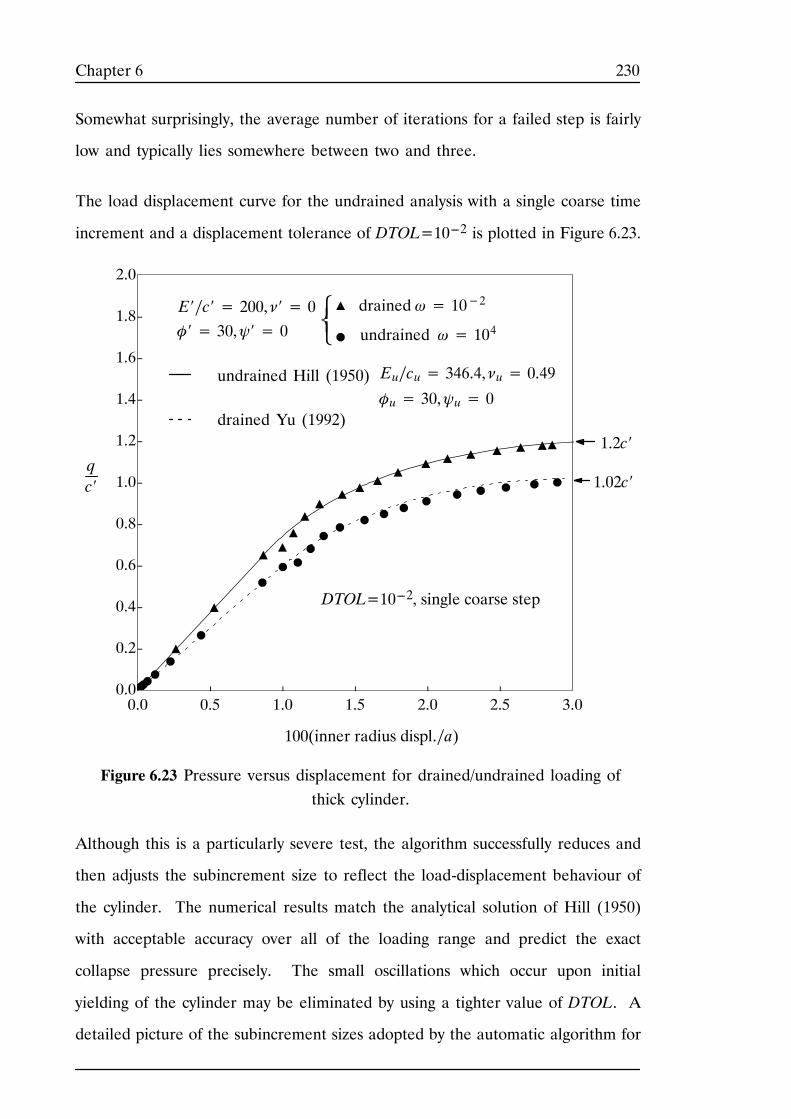
230Chapter 6
Somewhat surprisingly, the average number of iterations for a failed step is fairly
low and typically lies somewhere between two and three.
The load displacement curve for the undrained analysis with a single coarse time
increment and a displacement tolerance of DTOL=10---2 is plotted in Figure 6.23.
0.0
0.2
0.4
0.6
0.8
1.0
1.2
1.4
1.6
1.8
2.0
0.0 0.5 1.0 1.5 2.0 2.5 3.0
qc′
100(inner radius displ.∕a)
Figure 6.23 Pressure versus displacement for drained/undrained loading ofthick cylinder.
1.02c′
1.2c′
Eu∕cu= 346.4, νu= 0.49
undrained ω= 104
undrained Hill (1950)
DTOL=10---2, single coarse step
φu= 30,ψu= 0drained Yu (1992)
drained ω= 10−2E′∕c′ = 200, ν′ = 0φ′ = 30,ψ′ = 0 ⎨⎧⎩
Although this is a particularly severe test, the algorithm successfully reduces and
then adjusts the subincrement size to reflect the load-displacement behaviour of
the cylinder. The numerical results match the analytical solution of Hill (1950)
with acceptable accuracy over all of the loading range and predict the exact
collapse pressure precisely. The small oscillations which occur upon initial
yielding of the cylinder may be eliminated by using a tighter value of DTOL. A
detailed picture of the subincrement sizes adopted by the automatic algorithm for
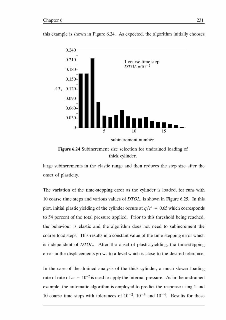
231Chapter 6
this example is shown in Figure 6.24. As expected, the algorithm initially chooses
0
0.030
0.060
0.090
0.120
0.150
0.180
0.210
0.240
5 10 15
ΔTv
Figure 6.24 Subincrement size selection for undrained loading ofthick cylinder.
subincrement number
1 coarse time stepDTOL=10---2
large subincrements in the elastic range and then reduces the step size after the
onset of plasticity.
The variation of the time-stepping error as the cylinder is loaded, for runs with
10 coarse time steps and various values of DTOL, is shown in Figure 6.25. In this
plot, initial plastic yielding of the cylinder occurs at q∕c′ = 0.65 which corresponds
to 54 percent of the total pressure applied. Prior to this threshold being reached,
the behaviour is elastic and the algorithm does not need to subincrement the
coarse load steps. This results in a constant value of the time-stepping error which
is independent of DTOL. After the onset of plastic yielding, the time-stepping
error in the displacements grows to a level which is close to the desired tolerance.
In the case of the drained analysis of the thick cylinder, a much slower loading
rate of rate of ω= 10–2 is used to apply the internal pressure. As in the undrained
example, the automatic algorithm is employed to predict the response using 1 and
10 coarse time steps with tolerances of 10---2, 10---3 and 10---4. Results for these
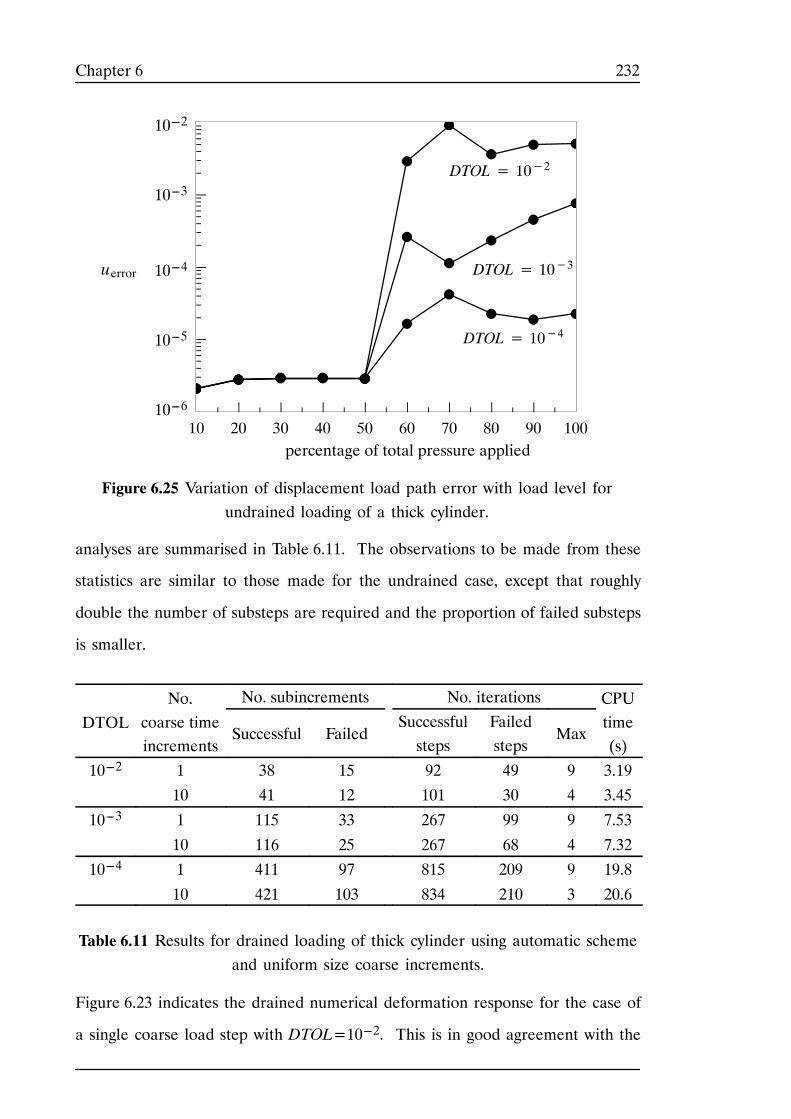
232Chapter 6
10 20 30 40 50 60 70 80 90 100
percentage of total pressure applied
Figure 6.25 Variation of displacement load path error with load level forundrained loading of a thick cylinder.
DTOL= 10−3
DTOL= 10−2
DTOL= 10−4
10---2
10---3
10---4
10---5
10---6
uerror
analyses are summarised in Table 6.11. The observations to be made from these
statistics are similar to those made for the undrained case, except that roughly
double the number of substeps are required and the proportion of failed substeps
is smaller.
No. No. subincrements No. iterations CPUDTOL
o.coarse timeincrements
Successful FailedSuccessfulsteps
Failedsteps
Max
C Utime(s)
10---2 1 38 15 92 49 9 3.1910 41 12 101 30 4 3.45
10---3 1 115 33 267 99 9 7.53
10 116 25 267 68 4 7.3210---4 1 411 97 815 209 9 19.8
10 421 103 834 210 3 20.6
Table 6.11 Results for drained loading of thick cylinder using automatic schemeand uniform size coarse increments.
Figure 6.23 indicates the drained numerical deformation response for the case of
a single coarse load step with DTOL=10---2. This is in good agreement with the
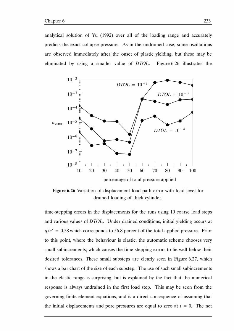
233Chapter 6
analytical solution of Yu (1992) over all of the loading range and accurately
predicts the exact collapse pressure. As in the undrained case, some oscillations
are observed immediately after the onset of plastic yielding, but these may be
eliminated by using a smaller value of DTOL. Figure 6.26 illustrates the
10 20 30 40 50 60 70 80 90 100
percentage of total pressure applied
Figure 6.26 Variation of displacement load path error with load level fordrained loading of thick cylinder.
DTOL= 10−3
DTOL= 10−2
DTOL= 10−4
10---2
10---3
10---4
10---5
10---6
10---7
10---8
uerror
time-stepping errors in the displacements for the runs using 10 coarse load steps
and various values of DTOL. Under drained conditions, initial yielding occurs at
q∕c′ = 0.58 which corresponds to 56.8 percent of the total applied pressure. Prior
to this point, where the behaviour is elastic, the automatic scheme chooses very
small subincrements, which causes the time-stepping errors to lie well below their
desired tolerances. These small substeps are clearly seen in Figure 6.27, which
shows a bar chart of the size of each substep. The use of such small subincrements
in the elastic range is surprising, but is explained by the fact that the numerical
response is always undrained in the first load step. This may be seen from the
governing finite element equations, and is a direct consequence of assuming that
the initial displacements and pore pressures are equal to zero at t= 0. The net
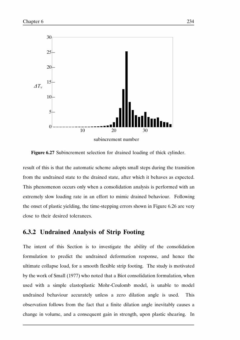
234Chapter 6
0
5
10
15
20
25
30
10 20 30
ΔTv
Figure 6.27 Subincrement selection for drained loading of thick cylinder.
subincrement number
result of this is that the automatic scheme adopts small steps during the transition
from the undrained state to the drained state, after which it behaves as expected.
This phenomenon occurs only when a consolidation analysis is performed with an
extremely slow loading rate in an effort to mimic drained behaviour. Following
the onset of plastic yielding, the time-stepping errors shown in Figure 6.26 are very
close to their desired tolerances.
6.3.2 Undrained Analysis of Strip Footing
The intent of this Section is to investigate the ability of the consolidation
formulation to predict the undrained deformation response, and hence the
ultimate collapse load, for a smooth flexible strip footing. The study is motivated
by the work of Small (1977) who noted that a Biot consolidation formulation, when
used with a simple elastoplastic Mohr-Coulomb model, is unable to model
undrained behaviour accurately unless a zero dilation angle is used. This
observation follows from the fact that a finite dilation angle inevitably causes a
change in volume, and a consequent gain in strength, upon plastic shearing. In
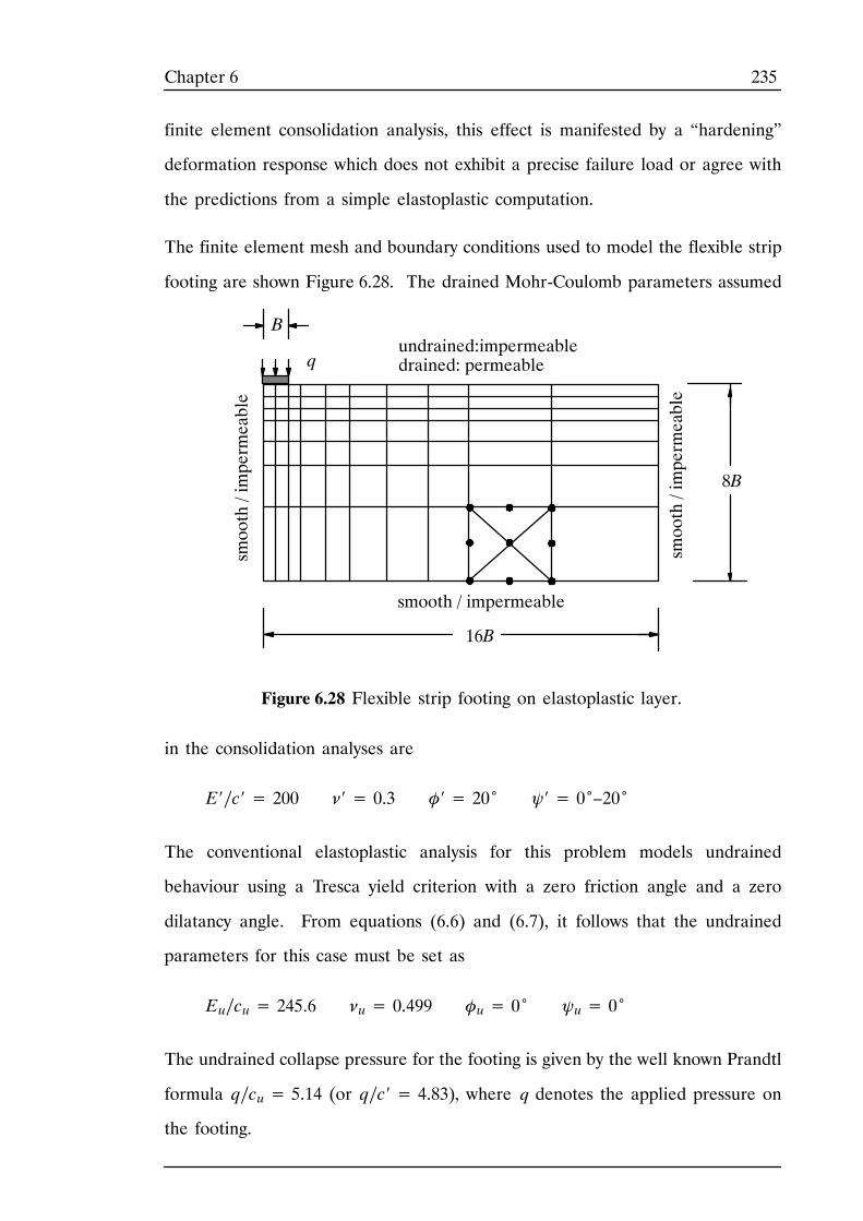
235Chapter 6
finite element consolidation analysis, this effect is manifested by a “hardening”
deformation response which does not exhibit a precise failure load or agree with
the predictions from a simple elastoplastic computation.
The finite element mesh and boundary conditions used to model the flexible strip
footing are shown Figure 6.28. The drained Mohr-Coulomb parameters assumed
undrained:impermeabledrained: permeable
16B
8B
B
Figure 6.28 Flexible strip footing on elastoplastic layer.
smooth/impermeable
smooth/impermeable
smooth / impermeable
q
in the consolidation analyses are
E′∕c′ = 200 ν′ = 0.3 φ′ = 20˚ ψ′ = 0˚–20˚
The conventional elastoplastic analysis for this problem models undrained
behaviour using a Tresca yield criterion with a zero friction angle and a zero
dilatancy angle. From equations (6.6) and (6.7), it follows that the undrained
parameters for this case must be set as
Eu∕cu= 245.6 νu= 0.499 φu= 0˚ ψu= 0˚
The undrained collapse pressure for the footing is given by the well known Prandtl
formula q∕cu= 5.14 (or q∕c′ = 4.83), where q denotes the applied pressure on
the footing.
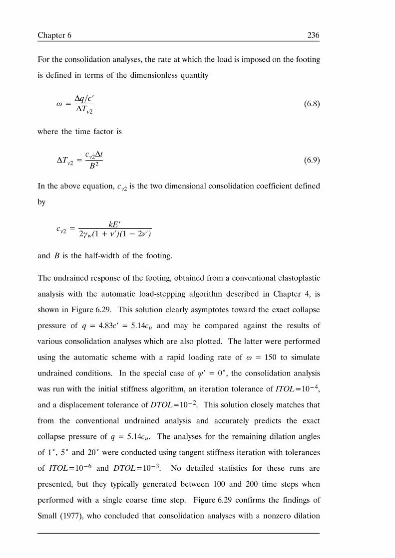
236Chapter 6
For the consolidation analyses, the rate at which the load is imposed on the footing
is defined in terms of the dimensionless quantity
ω=Δq∕c′ΔTv2
(6.8)
where the time factor is
ΔTv2=cv2ΔtB2
(6.9)
In the above equation, cv2 is the two dimensional consolidation coefficient defined
by
cv2=kE′
2γw(1+ ν′)(1− 2ν′)
and B is the half-width of the footing.
The undrained response of the footing, obtained from a conventional elastoplastic
analysis with the automatic load-stepping algorithm described in Chapter 4, is
shown in Figure 6.29. This solution clearly asymptotes toward the exact collapse
pressure of q= 4.83c′ = 5.14cu and may be compared against the results of
various consolidation analyses which are also plotted. The latter were performed
using the automatic scheme with a rapid loading rate of ω= 150 to simulate
undrained conditions. In the special case of ψ′ = 0˚, the consolidation analysis
was run with the initial stiffness algorithm, an iteration tolerance of ITOL=10---4,
and a displacement tolerance of DTOL=10---2. This solution closely matches that
from the conventional undrained analysis and accurately predicts the exact
collapse pressure of q= 5.14cu. The analyses for the remaining dilation angles
of 1˚, 5˚ and 20˚ were conducted using tangent stiffness iteration with tolerances
of ITOL=10---6 and DTOL=10---3. No detailed statistics for these runs are
presented, but they typically generated between 100 and 200 time steps when
performed with a single coarse time step. Figure 6.29 confirms the findings of
Small (1977), who concluded that consolidation analyses with a nonzero dilation
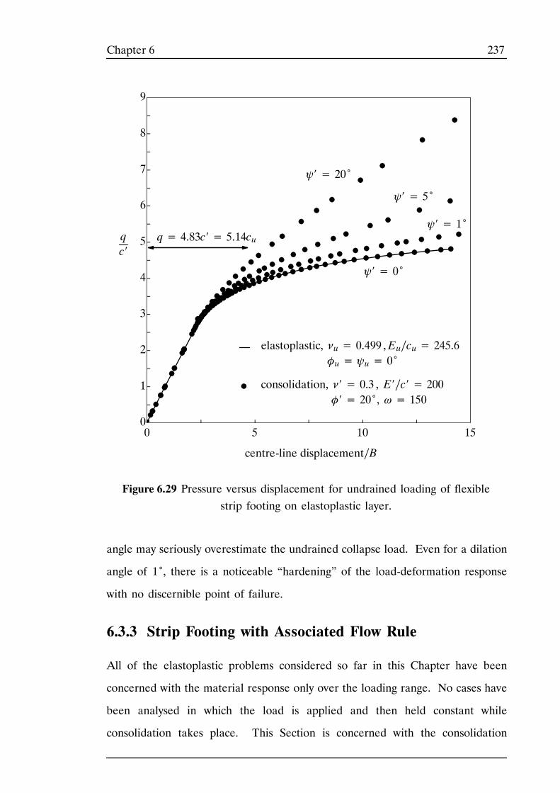
237Chapter 6
0
1
2
3
4
5
6
7
8
9
0 5 10 15
qc′
centre-line displacement∕B
Figure 6.29 Pressure versus displacement for undrained loading of flexiblestrip footing on elastoplastic layer.
ψ′ = 20˚
ψ′ = 1˚
ψ′ = 5˚
consolidation, ν′ = 0.3 , E′∕c′ = 200φ′ = 20˚, ω= 150
ψ′ = 0˚
elastoplastic, νu= 0.499 ,Eu∕cu= 245.6φu= ψu= 0˚
q= 4.83c′ = 5.14cu
angle may seriously overestimate the undrained collapse load. Even for a dilation
angle of 1 ,̊ there is a noticeable “hardening” of the load-deformation response
with no discernible point of failure.
6.3.3 Strip Footing with Associated Flow Rule
All of the elastoplastic problems considered so far in this Chapter have been
concerned with the material response only over the loading range. No cases have
been analysed in which the load is applied and then held constant while
consolidation takes place. This Section is concerned with the consolidation
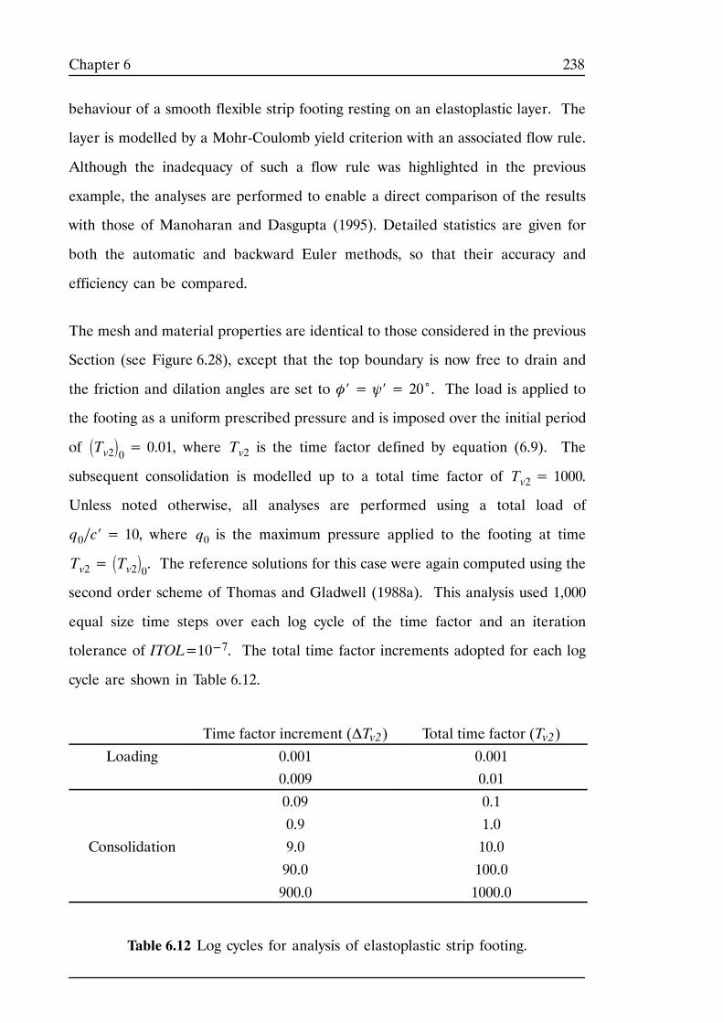
238Chapter 6
behaviour of a smooth flexible strip footing resting on an elastoplastic layer. The
layer is modelled by a Mohr-Coulomb yield criterion with an associated flow rule.
Although the inadequacy of such a flow rule was highlighted in the previous
example, the analyses are performed to enable a direct comparison of the results
with those of Manoharan and Dasgupta (1995). Detailed statistics are given for
both the automatic and backward Euler methods, so that their accuracy and
efficiency can be compared.
The mesh and material properties are identical to those considered in the previous
Section (see Figure 6.28), except that the top boundary is now free to drain and
the friction and dilation angles are set to φ′ = ψ′ = 20˚. The load is applied to
the footing as a uniform prescribed pressure and is imposed over the initial period
of Tv20= 0.01, where Tv2 is the time factor defined by equation (6.9). The
subsequent consolidation is modelled up to a total time factor of Tv2= 1000.
Unless noted otherwise, all analyses are performed using a total load of
q0∕c′ = 10, where q0 is the maximum pressure applied to the footing at time
Tv2= Tv20. The reference solutions for this case were again computed using the
second order scheme of Thomas and Gladwell (1988a). This analysis used 1,000
equal size time steps over each log cycle of the time factor and an iteration
tolerance of ITOL=10---7. The total time factor increments adopted for each log
cycle are shown in Table 6.12.
Time factor increment (ΔTv2) Total time factor (Tv2)
Loading 0.001 0.0010.009 0.01
0.09 0.1
0.9 1.0Consolidation 9.0 10.0
90.0 100.0
900.0 1000.0
Table 6.12 Log cycles for analysis of elastoplastic strip footing.
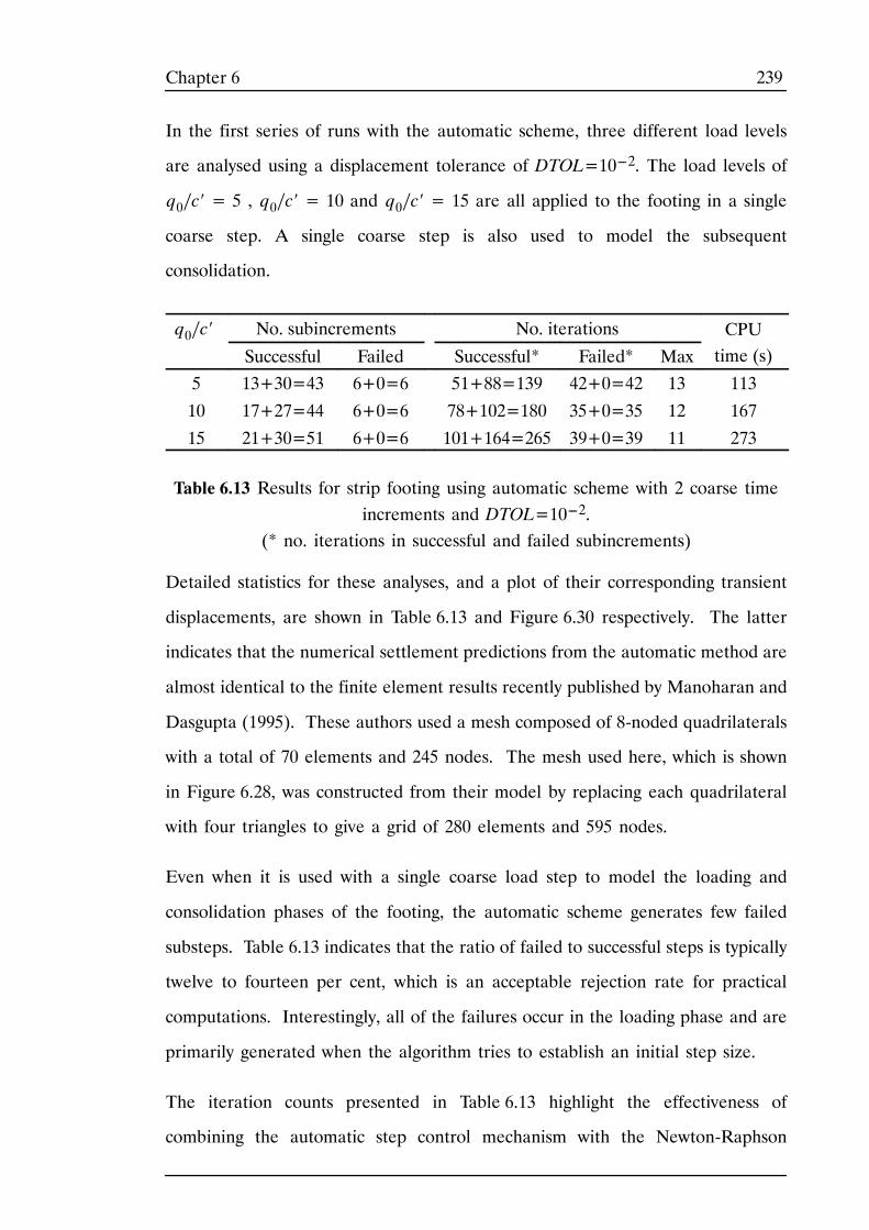
239Chapter 6
In the first series of runs with the automatic scheme, three different load levels
are analysed using a displacement tolerance of DTOL=10---2. The load levels of
q0∕c′ = 5 , q0∕c′ = 10 and q0∕c′ = 15 are all applied to the footing in a single
coarse step. A single coarse step is also used to model the subsequent
consolidation.
q0∕c′ No. subincrements No. iterations CPUSuccessful Failed Successful* Failed* Max time (s)
5 13+30=43 6+0=6 51+88=139 42+0=42 13 113
10 17+27=44 6+0=6 78+102=180 35+0=35 12 167
15 21+30=51 6+0=6 101+164=265 39+0=39 11 273
Table 6.13 Results for strip footing using automatic scheme with 2 coarse timeincrements and DTOL=10---2.
(* no. iterations in successful and failed subincrements)
Detailed statistics for these analyses, and a plot of their corresponding transient
displacements, are shown in Table 6.13 and Figure 6.30 respectively. The latter
indicates that the numerical settlement predictions from the automatic method are
almost identical to the finite element results recently published by Manoharan and
Dasgupta (1995). These authors used a mesh composed of 8-noded quadrilaterals
with a total of 70 elements and 245 nodes. The mesh used here, which is shown
in Figure 6.28, was constructed from their model by replacing each quadrilateral
with four triangles to give a grid of 280 elements and 595 nodes.
Even when it is used with a single coarse load step to model the loading and
consolidation phases of the footing, the automatic scheme generates few failed
substeps. Table 6.13 indicates that the ratio of failed to successful steps is typically
twelve to fourteen per cent, which is an acceptable rejection rate for practical
computations. Interestingly, all of the failures occur in the loading phase and are
primarily generated when the algorithm tries to establish an initial step size.
The iteration counts presented in Table 6.13 highlight the effectiveness of
combining the automatic step control mechanism with the Newton-Raphson
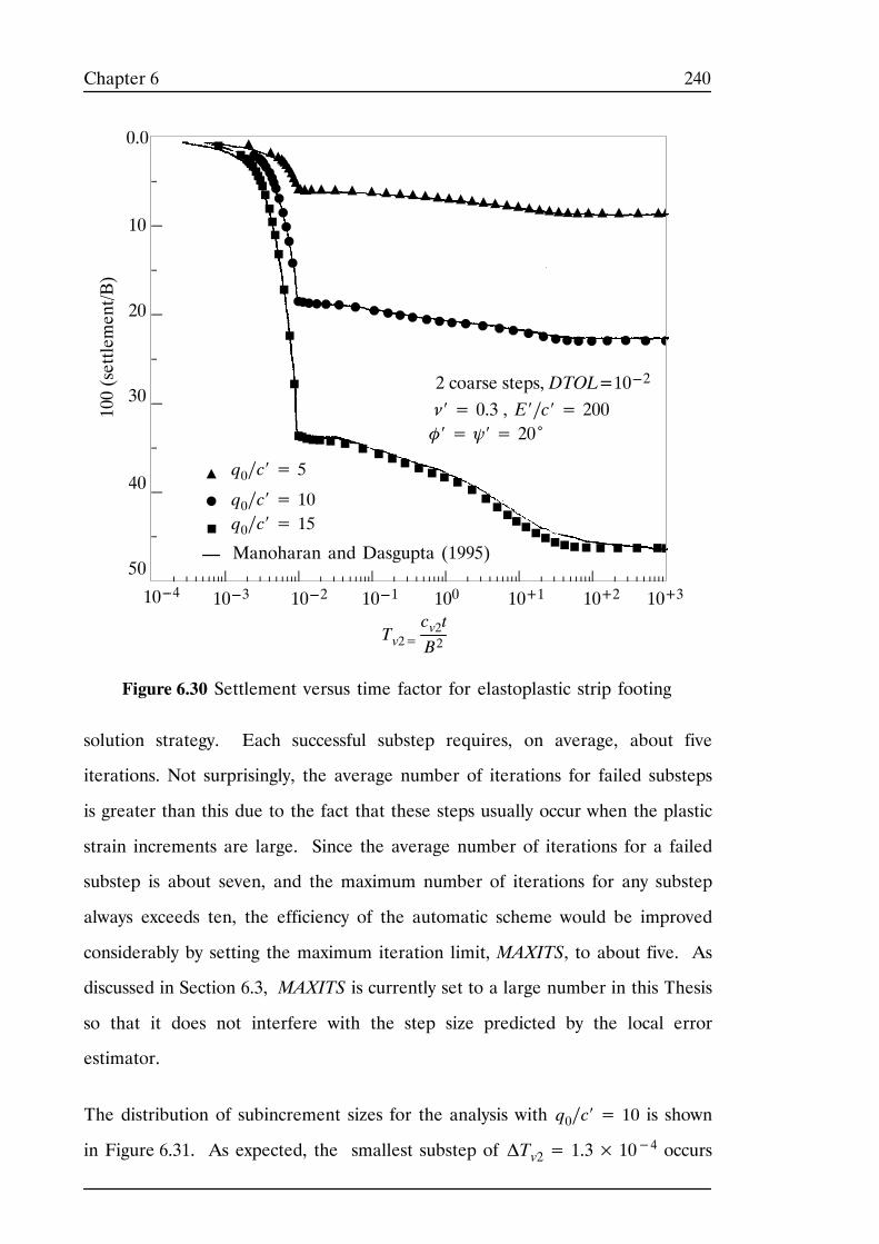
240Chapter 6
Figure 6.30 Settlement versus time factor for elastoplastic strip footing
Tv2=cv2t
B2
q0∕c′ = 5
q0∕c′ = 15q0∕c′ = 10
Manoharan and Dasgupta (1995)
10010---110---2 10+210---3 10+1 10+3
0.0
10
20
30
10---4
40
50
100(settlement/B)
ν′ = 0.3 , E′∕c′ = 200φ′ = ψ′ = 20˚
2 coarse steps, DTOL=10---2
solution strategy. Each successful substep requires, on average, about five
iterations. Not surprisingly, the average number of iterations for failed substeps
is greater than this due to the fact that these steps usually occur when the plastic
strain increments are large. Since the average number of iterations for a failed
substep is about seven, and the maximum number of iterations for any substep
always exceeds ten, the efficiency of the automatic scheme would be improved
considerably by setting the maximum iteration limit, MAXITS, to about five. As
discussed in Section 6.3, MAXITS is currently set to a large number in this Thesis
so that it does not interfere with the step size predicted by the local error
estimator.
The distribution of subincrement sizes for the analysis with q0∕c′ = 10 is shown
in Figure 6.31. As expected, the smallest substep of ΔTv2= 1.3× 10⁻⁴ occurs
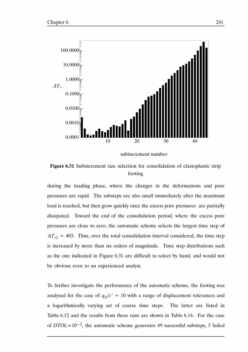
241Chapter 6
Figure 6.31 Subincrement size selection for consolidation of elastoplastic stripfooting
0.0001
0.0010
0.0100
0.1000
1.0000
10.0000
100.0000
10 20 30 40
ΔTv
subincrement number
during the loading phase, where the changes in the deformations and pore
pressures are rapid. The substeps are also small immediately after the maximum
load is reached, but then grow quickly once the excess pore pressures are partially
dissipated. Toward the end of the consolidation period, where the excess pore
pressures are close to zero, the automatic scheme selects the largest time step of
ΔTv2= 403. Thus, over the total consolidation interval considered, the time step
is increased by more than six orders of magnitude. Time step distributions such
as the one indicated in Figure 6.31 are difficult to select by hand, and would not
be obvious even to an experienced analyst.
To further investigate the performance of the automatic scheme, the footing was
analysed for the case of q0∕c′ = 10 with a range of displacement tolerances and
a logarithmically varying set of coarse time steps. The latter are listed in
Table 6.12 and the results from these runs are shown in Table 6.14. For the case
of DTOL=10---2, the automatic scheme generates 49 successful substeps, 5 failed
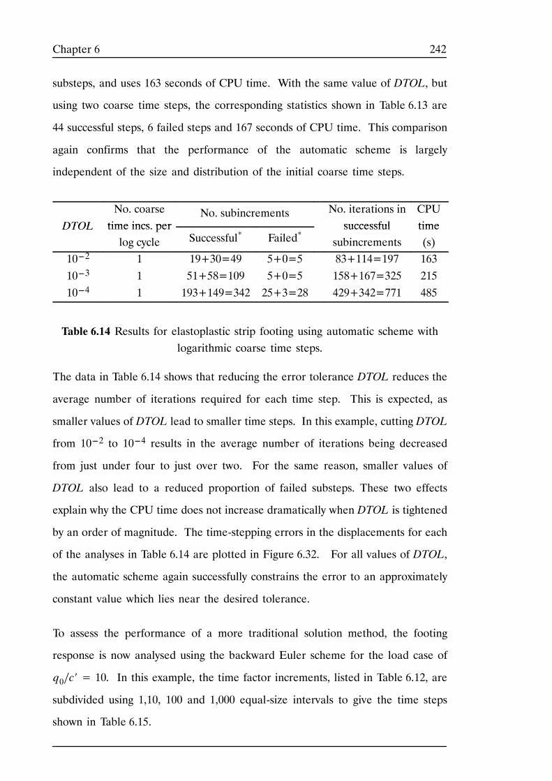
242Chapter 6
substeps, and uses 163 seconds of CPU time. With the same value of DTOL, but
using two coarse time steps, the corresponding statistics shown in Table 6.13 are
44 successful steps, 6 failed steps and 167 seconds of CPU time. This comparison
again confirms that the performance of the automatic scheme is largely
independent of the size and distribution of the initial coarse time steps.
DTOLNo. coarsetime incs per
No. subincrements No. iterations insuccessful
CPUtimeDTOL time incs. per
log cycle Successful* Failed*successfulsubincrements
time(s)
10---2 1 19+30=49 5+0=5 83+114=197 16310---3 1 51+58=109 5+0=5 158+167=325 21510---4 1 193+149=342 25+3=28 429+342=771 485
Table 6.14 Results for elastoplastic strip footing using automatic scheme withlogarithmic coarse time steps.
The data in Table 6.14 shows that reducing the error tolerance DTOL reduces the
average number of iterations required for each time step. This is expected, as
smaller values of DTOL lead to smaller time steps. In this example, cutting DTOL
from 10---2 to 10---4 results in the average number of iterations being decreased
from just under four to just over two. For the same reason, smaller values of
DTOL also lead to a reduced proportion of failed substeps. These two effects
explain why the CPU time does not increase dramatically when DTOL is tightened
by an order of magnitude. The time-stepping errors in the displacements for each
of the analyses in Table 6.14 are plotted in Figure 6.32. For all values of DTOL,
the automatic scheme again successfully constrains the error to an approximately
constant value which lies near the desired tolerance.
To assess the performance of a more traditional solution method, the footing
response is now analysed using the backward Euler scheme for the load case of
q0∕c′ = 10. In this example, the time factor increments, listed in Table 6.12, are
subdivided using 1,10, 100 and 1,000 equal-size intervals to give the time steps
shown in Table 6.15.
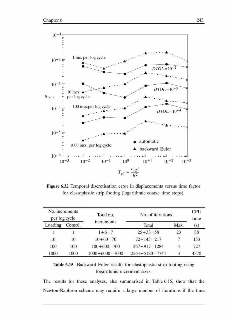
243Chapter 6
Tv2=cv2 tB2
100 incs.per log cycle
10 incs.per log cycle
1000 incs. per log cycle
Figure 6.32 Temporal discretisation error in displacements versus time factorfor elastoplastic strip footing (logarithmic coarse time steps).
10010---110---2 10+210---3 10+1 10+3
10---2
10---3
10---4
10---5
10---6backward Euler
automatic
uerror
DTOL=10---4
DTOL=10---3
DTOL=10---2
10---1
1 inc. per log cycle
No. incrementsper log cycle
Total no.increments
No. of iterationsCPUtime
Loading Consol.increments
Total Max. (s)1 1 1+6=7 25+33=58 23 88
10 10 10+60=70 72+145=217 7 153
100 100 100+600=700 367+917=1284 4 7271000 1000 1000+6000=7000 2564+5180=7744 3 4370
Table 6.15 Backward Euler results for elastoplastic strip footing usinglogarithmic increment sizes.
The results for these analyses, also summarised in Table 6.15, show that the
Newton-Raphson scheme may require a large number of iterations if the time
244Chapter 6
discretisation is very coarse. For the crudest analysis with one time step in the
loading phase and six time steps in the consolidation phase, up to 23 iterations are
needed to reach convergence and the average iteration count is just over eight.
This is in contrast to the 7000 increment run which gives maximum and average
iteration counts of three and one respectively. As expected, the largest average
iteration counts for all the analyses occur during the loading phase. Figure 6.32
summarises the temporal discretisation error at the end of each log cycle of the
time factor for the various runs. This plot indicates that even with the crudest
discretisation of one time step per log cycle, the backward Euler method gives a
time-stepping error of just two percent. The results also confirm the expected first
order accuracy of this type of solution strategy.
The results in Table 6.14, Table 6.15 and Figure 6.32 can be used to compare the
relative efficiency of the automatic and backward Euler methods for the footing
problem. The Figure indicates that these two schemes, when used with
DTOL=10---2 and one increment per log cycle, respectively, give similar maximum
time stepping errors. The CPU time for the backward Euler method, however,
is only 88 seconds as opposed to 163 seconds for the automatic scheme. For more
accurate analyses, the relative performance of the automatic scheme improves
significantly and is competitive with that of the backward Euler algorithm. This
can be seen by comparing the timing statistics for the automatic analysis with
DTOL=10---4 against the timing statistics for the 700 increment backward Euler
run. The former, although marginally more accurate, requires only 485 CPU
seconds as opposed to 727 CPU seconds for the latter, a saving of approximately
33 percent. When making this type of comparison, it should be remembered that
the backward Euler scheme will usually need to be run with a range of different
time steps in order to determine when the time-stepping error is negligible. The
automatic scheme, however, need only be run once.
245Chapter 6
6.3.4 Strip Footing with Nonassociated Flow Rule
The results shown in Section 6.3.2 highlighted the need to employ a nonassociated
flow rule when using a simple Mohr-Coulomb model with a Biot consolidation
formulation. In particular, it is necessary to use a non-dilatant flow rule to obtain
solutions which match those from a conventional elastoplastic analysis for the
limiting case of undrained loading. This Section examines the ability of the
consolidation formulation to accurately predict the drained collapse pressure for
a flexible strip footing subjected to a very slow rate of loading. The important
influence of the iteration tolerance on the efficiency of the initial stiffness
algorithm is also investigated.
The geometry, boundary conditions and finite element mesh for the footing are
identical to those used in the preceding example (see Figure 6.28). The drained
soil parameters adopted for the Mohr-Coulomb model are similar to those
employed in Section 6.3.2, except that the dilation angle is always zero. Thus
E′∕c′ = 20 ν′ = 0.3 φ′ = 20˚ ψ′ = 0˚
and the corresponding Prandtl collapse pressure is q∕c′ = 14.83. The
conventional elastoplastic analysis for this problem uses the above parameters, and
the rounded Mohr-Coulomb yield surface described in Chapter 2, to model the
drained state. One thousand equal size pressure increments are imposed on the
footing and an initial stiffness algorithm is employed to solve the governing
equations. The automatic load-stepping scheme of Chapter 4 could not be used
for this case, as the tangent stiffness matrix becomes ill-conditioned when ψ′ = 0.
The consolidation analyses are performed with loading rate values ranging from
ω= 0.015 to ω= 150, where ω is again defined by equation (6.8). The former
case generates very small excess pore pressures and thus models the drained
condition very closely. As shown in Section 6.3.2, the higher setting accurately
simulates undrained loading. All of the consolidation runs are performed with two
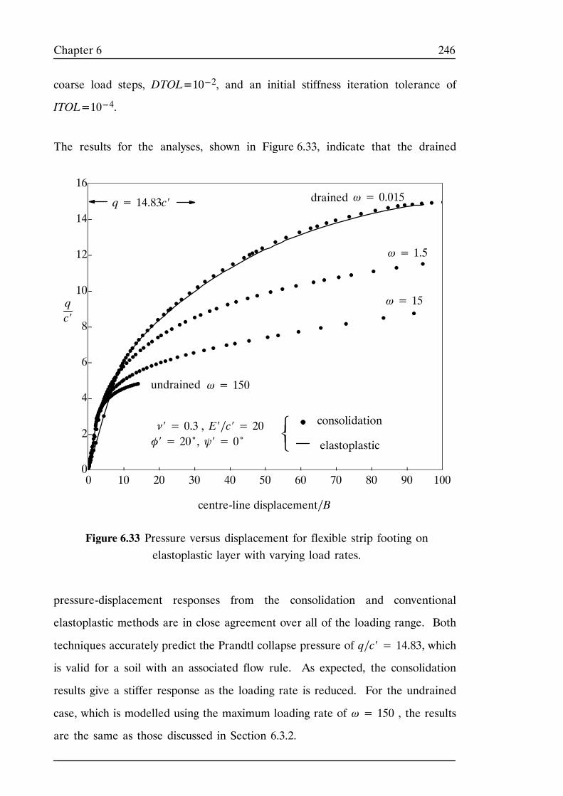
246Chapter 6
coarse load steps, DTOL=10---2, and an initial stiffness iteration tolerance of
ITOL=10---4.
The results for the analyses, shown in Figure 6.33, indicate that the drained
0
2
4
6
8
10
12
14
16
0 10 20 30 40 50 60 70 80 90 100
elastoplastic
ν′ = 0.3 , E′∕c′ = 20φ′ = 20˚, ψ′ = 0˚
consolidation
qc′
Figure 6.33 Pressure versus displacement for flexible strip footing onelastoplastic layer with varying load rates.
undrained
drained
ω= 150
ω= 15
ω= 0.015
ω= 1.5
centre-line displacement∕B
⎨⎧⎩
q= 14.83c′
pressure-displacement responses from the consolidation and conventional
elastoplastic methods are in close agreement over all of the loading range. Both
techniques accurately predict the Prandtl collapse pressure of q∕c′ = 14.83, which
is valid for a soil with an associated flow rule. As expected, the consolidation
results give a stiffer response as the loading rate is reduced. For the undrained
case, which is modelled using the maximum loading rate of ω= 150 , the results
are the same as those discussed in Section 6.3.2.
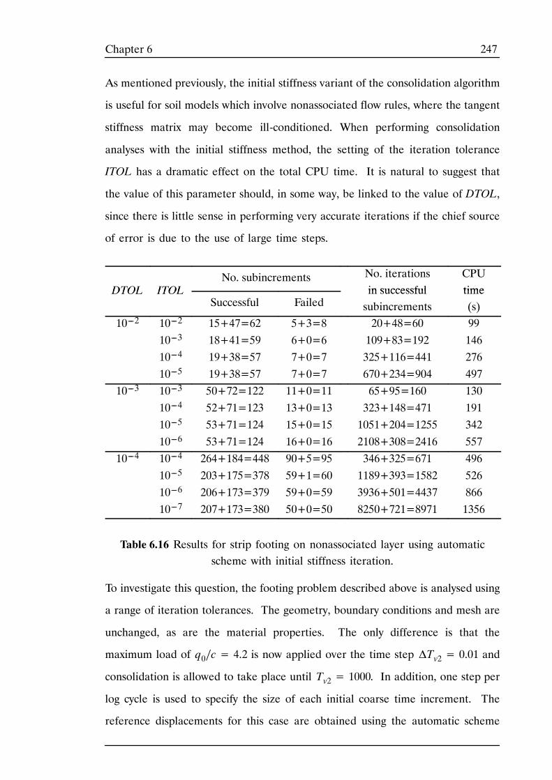
247Chapter 6
As mentioned previously, the initial stiffness variant of the consolidation algorithm
is useful for soil models which involve nonassociated flow rules, where the tangent
stiffness matrix may become ill-conditioned. When performing consolidation
analyses with the initial stiffness method, the setting of the iteration tolerance
ITOL has a dramatic effect on the total CPU time. It is natural to suggest that
the value of this parameter should, in some way, be linked to the value of DTOL,
since there is little sense in performing very accurate iterations if the chief source
of error is due to the use of large time steps.
DTOL ITOLNo. subincrements No. iterations
in successfulCPUtimeDTOL ITOL
Successful Failedin successfulsubincrements
time(s)
10---2 10---2 15+47=62 5+3=8 20+48=60 9910---3 18+41=59 6+0=6 109+83=192 14610---4 19+38=57 7+0=7 325+116=441 27610---5 19+38=57 7+0=7 670+234=904 497
10---3 10---3 50+72=122 11+0=11 65+95=160 13010---4 52+71=123 13+0=13 323+148=471 19110---5 53+71=124 15+0=15 1051+204=1255 34210---6 53+71=124 16+0=16 2108+308=2416 557
10---4 10---4 264+184=448 90+5=95 346+325=671 49610---5 203+175=378 59+1=60 1189+393=1582 52610---6 206+173=379 59+0=59 3936+501=4437 86610---7 207+173=380 50+0=50 8250+721=8971 1356
Table 6.16 Results for strip footing on nonassociated layer using automaticscheme with initial stiffness iteration.
To investigate this question, the footing problem described above is analysed using
a range of iteration tolerances. The geometry, boundary conditions and mesh are
unchanged, as are the material properties. The only difference is that the
maximum load of q0∕c= 4.2 is now applied over the time step ΔTv2= 0.01 and
consolidation is allowed to take place until Tv2= 1000. In addition, one step per
log cycle is used to specify the size of each initial coarse time increment. The
reference displacements for this case are obtained using the automatic scheme
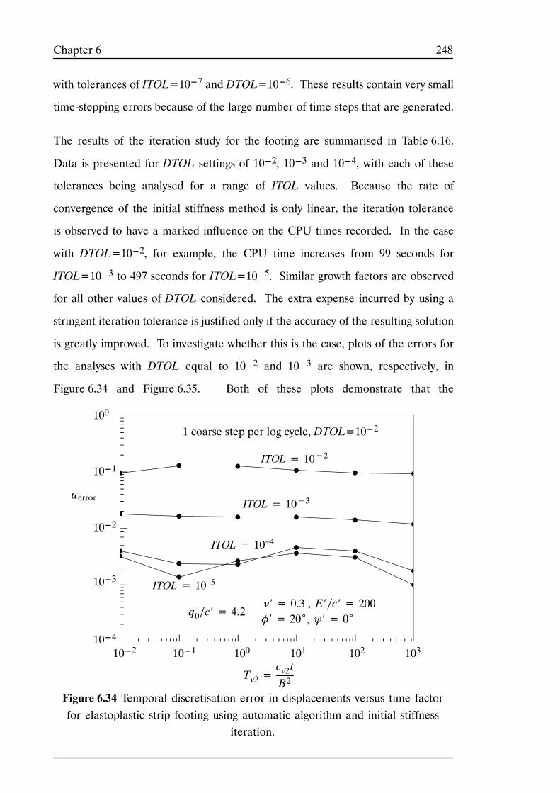
248Chapter 6
with tolerances of ITOL=10---7 and DTOL=10---6. These results contain very small
time-stepping errors because of the large number of time steps that are generated.
The results of the iteration study for the footing are summarised in Table 6.16.
Data is presented for DTOL settings of 10---2, 10---3 and 10---4, with each of these
tolerances being analysed for a range of ITOL values. Because the rate of
convergence of the initial stiffness method is only linear, the iteration tolerance
is observed to have a marked influence on the CPU times recorded. In the case
with DTOL=10---2, for example, the CPU time increases from 99 seconds for
ITOL=10---3 to 497 seconds for ITOL=10---5. Similar growth factors are observed
for all other values of DTOL considered. The extra expense incurred by using a
stringent iteration tolerance is justified only if the accuracy of the resulting solution
is greatly improved. To investigate whether this is the case, plots of the errors for
the analyses with DTOL equal to 10---2 and 10---3 are shown, respectively, in
Figure 6.34 and Figure 6.35. Both of these plots demonstrate that the
Tv2=cv2 tB2
Figure 6.34 Temporal discretisation error in displacements versus time factorfor elastoplastic strip footing using automatic algorithm and initial stiffness
iteration.
ITOL= 10–4
ITOL= 10–5
ITOL= 10−2
ITOL= 10−3
10010---110---2
100
10---1
10---2
10---3
101 10310210---4
q0∕c′ = 4.2
uerror
ν′ = 0.3 , E′∕c′ = 200φ′ = 20˚, ψ′ = 0˚
1 coarse step per log cycle, DTOL=10---2
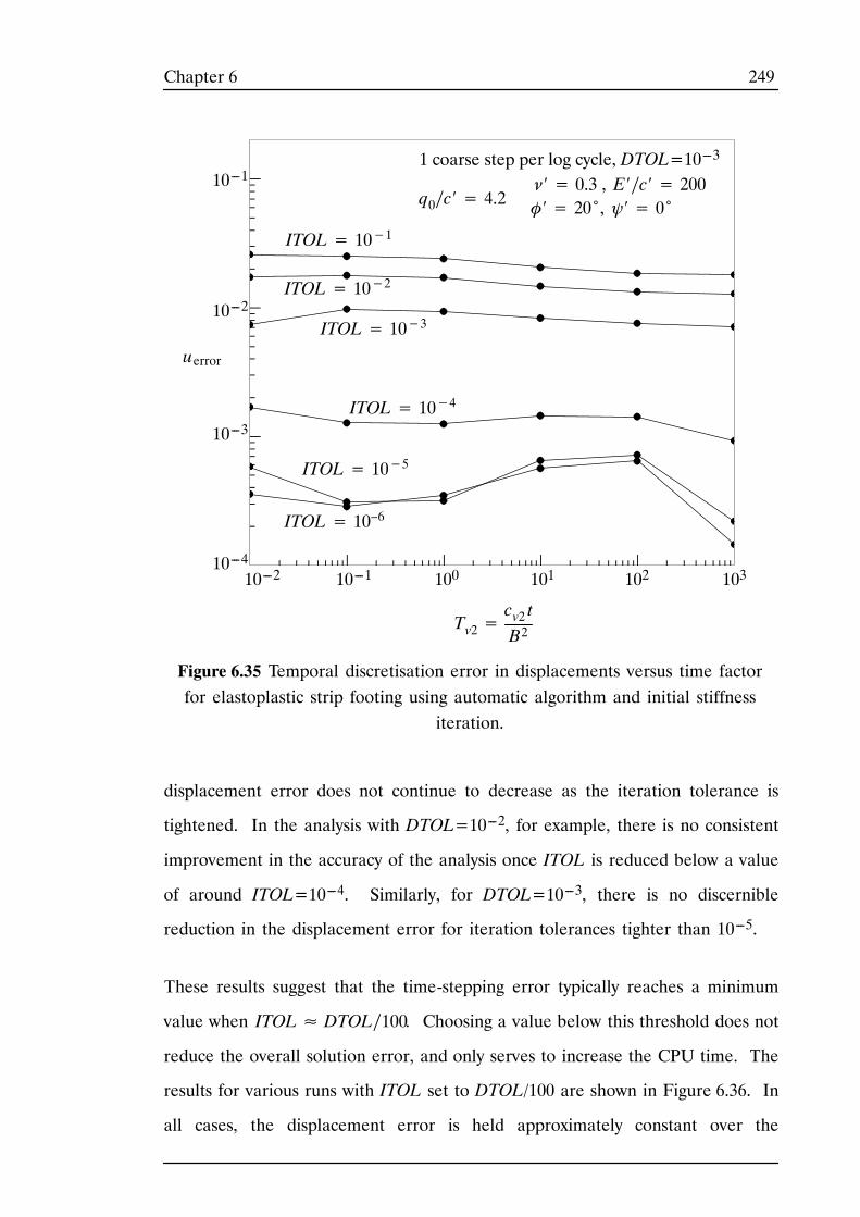
249Chapter 6
Figure 6.35 Temporal discretisation error in displacements versus time factorfor elastoplastic strip footing using automatic algorithm and initial stiffness
iteration.
ITOL= 10–6
ITOL= 10−4
ITOL= 10−5
Tv2=cv2 tB2
ITOL= 10−3
ITOL= 10−1
ITOL= 10−2
10010---110---2
10---1
10---2
10---3
10---4101 103102
uerror
q0∕c′ = 4.2ν′ = 0.3 , E′∕c′ = 200φ′ = 20˚, ψ′ = 0˚
1 coarse step per log cycle, DTOL=10---3
displacement error does not continue to decrease as the iteration tolerance is
tightened. In the analysis with DTOL=10---2, for example, there is no consistent
improvement in the accuracy of the analysis once ITOL is reduced below a value
of around ITOL=10---4. Similarly, for DTOL=10---3, there is no discernible
reduction in the displacement error for iteration tolerances tighter than 10---5.
These results suggest that the time-stepping error typically reaches a minimum
value when ITOL≈ DTOL∕100. Choosing a value below this threshold does not
reduce the overall solution error, and only serves to increase the CPU time. The
results for various runs with ITOL set to DTOL/100 are shown in Figure 6.36. In
all cases, the displacement error is held approximately constant over the
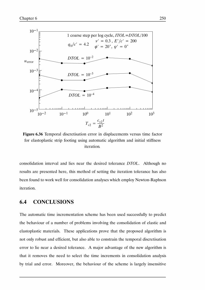
250Chapter 6
Tv2=cv2 tB2
Figure 6.36 Temporal discretisation error in displacements versus time factorfor elastoplastic strip footing using automatic algorithm and initial stiffness
iteration.
DTOL= 10–3
DTOL= 10–2
DTOL= 10–4
10010---110---2
10---1
10---2
10---3
10---4
10---5101 103102
uerror
q0∕c′ = 4.2ν′ = 0.3 , E′∕c′ = 200φ′ = 20˚, ψ′ = 0˚
1 coarse step per log cycle, ITOL=DTOL/100
consolidation interval and lies near the desired tolerance DTOL. Although no
results are presented here, this method of setting the iteration tolerance has also
been found to work well for consolidation analyses which employ Newton-Raphson
iteration.
6.4 CONCLUSIONS
The automatic time incrementation scheme has been used successfully to predict
the behaviour of a number of problems involving the consolidation of elastic and
elastoplastic materials. These applications prove that the proposed algorithm is
not only robust and efficient, but also able to constrain the temporal discretisation
error to lie near a desired tolerance. A major advantage of the new algorithm is
that it removes the need to select the time increments in consolidation analysis
by trial and error. Moreover, the behaviour of the scheme is largely insensitive
251Chapter 6
to the size and distribution of the coarse time steps that are required to start the
analysis.
The pitfalls of adopting an associated Mohr-Coulomb model in consolidation
analysis have been highlighted. For rapid rates of loading, this yield surface should
be used with a nonassociated flow rule and a zero angle of dilatancy to obtain
reliable predictions of soil behaviour.
Finally, it was shown that there is little benefit in using excessively stringent
iteration tolerances in elastoplastic consolidation calculations. For the automatic
scheme, a simple rule is proposed which ties the value of the iteration tolerance
to the displacement error tolerance. This rule helps to minimise the number of
wasted iterations, yet ensures that the desired accuracy requirements are met.

252Chapter 6
253Chapter 7
CHAPTER 7
CONCLUDING REMARKS
254Chapter 7
7.1 SUMMARY
In this Thesis, various algorithms for finite element analysis of consolidation and
elastoplasticity have been developed. This includes the derivation of a smooth
approximation to the Mohr-Coulomb yield criterion which has no singularities in
its gradient. The main thrust of this Thesis, however, has been concerned with
the development of techniques for controlling the linearisation error which is
caused by the use of finite size steps in the solution of nonlinear problems. This
work can be divided in to three distinct areas; namely, the integration of
elastoplastic stress-strain laws, the solution of the governing load-deflection
relations of elastoplasticity, and the solution of the coupled equations of
elastoplastic consolidation.
7.2 ROUNDED APPROXIMATION TO THEMOHR-COULOMB YIELD CRITERION
In Chapter 2, a fully rounded approximation to the Mohr-Coulomb yield criterion
was derived. The new yield criterion, which uses a trigonometric approximation
in the octahedral plane and a hyperbolic approximation in the Meridional plane,
eliminates all gradient singularities from the Mohr-Coulomb yield criterion. The
resulting yield surface is both continuous and differentiable at all stress states and
is able to model the true Mohr-Coulomb yield surface as closely as desired by
adjusting only two parameters. The approximation is designed so that the true
Mohr-Coulomb yield criterion can be recovered as a special case.
The use of the smooth yield criterion in finite element computations avoids many
of the numerical difficulties that arise due to discontinuous gradients. In
particular, the integration of the constitutive relationships, the correction of stress
states to the yield surface, and the calculation of the stiffness matrices is
straightforward.
255Chapter 7
7.3 INTEGRATION OF ELASTOPLASTICCONSTITUTIVE LAWS
In Chapter 3, a number of important refinements to enhance the efficiency and
robustness of the explicit integration scheme of Sloan (1987) were developed.
These enhancements include improved algorithms for determining the intersection
to the yield surface, handling a negative plastic multiplier, and the correction of
stresses which drift from the yield surface during integration. By using a measure
of the local truncation error, the explicit modified Euler scheme automatically
subincrements the applied strain increments if a specified error tolerance is
exceeded. The advantage of this approach is that the error in the integration of
the constitutive law can be controlled using a rational method.
In the remainder of Chapter 3, the performance of the adaptive modified Euler
scheme is compared to that of the implicit backward Euler return scheme. As part
of this comparison, the performance of an explicit single step forward Euler
scheme and a single step implicit backward Euler scheme were also considered.
Both of these schemes are common in the analysis of elastoplasticity.
The performance of the single step schemes for the Tresca and Mohr-Coulomb
constitutive relationships is similar, and thus there is little to distinguish between
the two. The accuracy of these schemes is also comparable to the more
complicated modified Euler and backward Euler return procedures when the
strain increments are not excessively large. Hence, for simple yield criteria with
small load increments, explicit and implicit single step algorithms provide an
accurate and efficient solution. These methods, however, are unsuitable for
problems that are loaded in the fully plastic range.
The adaptive modified Euler and implicit backward Euler return schemes both
provide an economical means of integrating rounded Tresca and Mohr-Coulomb
constitutive laws. Each procedure requires a similar amount of CPU time and give
stresses of a similar accuracy. The explicit modified Euler scheme, however, has
256Chapter 7
the added advantage that the error in the computed stresses may be controlled to
a desired level. This is of particular benefit when analysing highly nonlinear
problems where large strain increments may be encountered.
A further advantage of the explicit modified Euler scheme is its robustness.
Because the technique is non-iterative and unconditionally stable, it can be used
to integrate complicated constitutive laws with large strain increments. In contrast,
the implicit backward Euler return scheme is less reliable and convergence
problems can and do arise in the iterative process. A robust implementation of
this scheme must also use a simple substepping strategy to ensure convergence.
The substepping strategy used in this Thesis enabled large strain increments to be
integrated efficiently without fear of numerical difficulty. When applied to the
rounded Mohr-Coulomb yield function without substepping, the implicit backward
Euler method may require very small load steps in order to ensure convergence
of the iteration scheme. The results for the footing problems suggest that the
implicit schemes do not perform well in the vicinity of the corners of the Tresca
and Mohr-Coulomb yield criteria, even when they are rounded, and special
strategies may be required.
A final attraction of the adaptive explicit method is that it requires only first
derivatives (with respect to the stresses) of the yield surface and plastic potential.
The second derivatives needed for the implicit methods are both difficult and
expensive to compute for many geotechnical models.
7.4 SOLUTION OF ELASTOPLASTICLOAD-DISPLACEMENT RELATIONS
In Chapter 4, a scheme for the automatic solution of the governing load deflection
equations in elastoplasticity was developed. The aim of this scheme was to control
the linearisation error that arises due to the use of finite size load increments.
The scheme, which is non-iterative and treats the governing relationships as a
system of ordinary differential equations, is structured so that user defined coarse
257Chapter 7
load increments are automatically subdivided into smaller subincrements. The
size of these subincrements is chosen so as to hold the local truncation error in
each step of the solution to below a user specified tolerance. The truncation error
is measured by taking the difference between incremental solutions obtained from
the first order accurate Euler scheme and the second order accurate modified
Euler scheme. By extrapolating the local error estimate, the algorithm is able to
expand or contract the size of the subincrements to reflect the nonlinearity of the
solution. For subincrements in which the local truncation error exceeds the
specified tolerance, the load step is abandoned and the integration repeated using
a smaller subincrement. Otherwise, the subincrement is accepted, the solution
advanced, and a new subincrement size predicted.
The performance of the explicit modified Euler scheme was demonstrated through
the analysis of several elastoplastic boundary value problems. The scheme was
able to solve the governing relations so that the load path error in the final
displacements lies near the desired tolerance. Generally, the error in the
displacements was constrained to within an order of magnitude of the desired
tolerance. The technique controlled this error independently of the number of
coarse load increments supplied by the user. Even for the most severe analyses
in which the total load was specified as a single coarse increment, the scheme
successfully adjusted the subincrement sizes to achieve the specified accuracy in
the solution.
The speed of the automatic error control scheme compared favourably with the
conventional forward Euler scheme. Indeed, the average CPU time per step for
these two methods differed only marginally. The chief benefit of the automatic
scheme is that it removes the guess work involved in specifying the load increments
by hand. Moreover, it only uses small load increments where necessary. The
benefits of using an adaptive incrementation scheme were demonstrated by
considering the size and distribution of the automatically generated subincrements.
258Chapter 7
In the analysis of the thick cylinder, the automatic scheme maintained a constant
error in the solution by using uniform size increments throughout the range of
plastic deformation. The analysis of the trapdoor problem, however, resulted in
a series of subincrements which expanded in size throughout the loading range.
The new automatic scheme can be applied to a wide range of nonlinear problems,
not just those that occur in plasticity. The algorithm is particularly robust, and
can only fail if the tangent stiffness matrix becomes singular.
7.5 SOLUTION OF THE GOVERNING EQUATIONS INCONSOLIDATION
Chapter 5 details the development of automatic time stepping algorithms for
solving elastic and elastoplastic coupled consolidation problems. Unlike the other
governing equations considered in this Thesis, the governing equations of
consolidation are coupled and require the use of implicit integration methods to
ensure unconditionally stability. The procedures developed in Chapter 5 treat the
governing consolidation relations as a system of first order differential equations
and are based on the backward Euler method and the Thomas and Gladwell
(1988a) method. By choosing the integration parameters for these two methods
judiciously, the local truncation error for each time step can be computed very
cheaply. This permits the time steps to be controlled in a manner similar to that
developed for the governing equations of elastoplasticity. The automatic
consolidation algorithm operates by subdividing a series of user defined coarse
time increments and limits the local truncation error in the displacements to less
than a user specified tolerance. For the elastic case, the displacements and pore
pressures at the end of each subincrement are solved directly without the need for
iteration. For elastoplastic behaviour, however, the governing relationships are
nonlinear and a system of nonlinear equations must be solved to compute the
updates.
259Chapter 7
In Chapter 6, the automatic consolidation algorithm was applied to several
problems concerning the consolidation of elastic and elastoplastic materials. In
all cases, the scheme was able to constrain the global temporal error in the
displacements to lie near the desired tolerance. The elastoplastic thick cylinder
analysis confirmed the accuracy of the consolidation formulation for the limiting
cases of undrained and undrained behaviour. The example of a rapidly loaded
strip footing highlighted the need to use the Mohr-Coulomb yield surface with a
nonassociated flow rule for undrained conditions. In the last part of the Chapter,
other strip footing examples further confirmed the accuracy and speed of the
automatic consolidation formulation. All of the cases considered prove that the
behaviour of the automatic procedure is largely insensitive to the size and
distribution of the initial coarse time steps.
The performance of the automatic consolidation scheme compares favourably to
that of the conventional backward Euler scheme. To achieve solutions of similar
accuracy, the automatic and backward Euler schemes use a similar amount of
computational effort. The backward Euler scheme is marginally faster for a crude
analysis while the automatic scheme is much faster when an accurate solution is
required. The chief advantage of the automatic method is that it removes the need
to determine the time stepping error by an empirical trial and error procedure.

260Chapter 7
261References
REFERENCES
262References
Bell, A.L., ‘The lateral pressure and resistance of clay and the supporting power
of clay foundations’, Proc. I.C.E., 199, 223, 1915
Bergan, P.G, Horrigmoe, G., Krakeland, B. and Soreide, T.H., ‘Solution techniques
for nonlinear finite element problems’, International Journal for
Numerical Methods in Engineering, 12, 1677-1696, 1978
Bergan, P.G. and Soreide, T., ‘Solution of large displacement and instability
problems using the current stiffness parameter’, in Finite Elements in
Nonlinear Mechanics (Eds P.G. Bergan et al.) Tapir Press, 1978
Biot, M.A., ‘General theory of three dimensional consolidation’, Journal of Applied
Physics, 12, 155-164, 1941a
Biot, M.A., ‘Consolidation under a rectangular load distribution’, Journal of
Applied Physics, 12, 426-430, 1941b
Biot, M.A., ‘Theory of elasticity and consolidation for a porous anisotropic solid’,
Journal of Applied Physics, 26, 182-185, 1955
Biot, M.A., ‘General solution of the equation of elasticity and consolidation for
a porous material’, Journal of Applied Mechanics, 23, 91-96, 1956a
Biot, M.A., ‘Theory of deformation of a porous viscoelastic anisotropic solid’,
Journal of Applied Physics, 27, 459-467, 1956b
Biot, M.A., ‘Theory of stability and consolidation of a porous medium under initial
stress’, Journal of Mathematics and Mechanics, 12, 521-541, 1963
Booker, J.R. ‘The consolidation of a finite layer subject to surface loading’,
International Journal for Solids and Structures, 10, 1053-1065, 1974
Booker, J.R. and Small, J.C., ‘An investigation of the stability of numerical
solutions of Biot’s equations of consolidation’, International Journal of
Solids and Structures, 11, 907-917, 1975
263References
Borja, R.I., ‘Finite element formulation for transient pore pressure dissipation: A
variational approach’, International Journal of Solids and Structures, 22,
1201-1211, 1986
Borja, R.I., ‘Linearisation of elasto-plastic consolidation equations’, Engineering
Computations, 6, 163-168, 1989
Borja, R.I., ‘One-step and linear multistep methods for nonlinear consolidation’,
Computer Methods in Applied Mechanics and Engineering, 85, 239-272,
1991
Borja, R.I., ‘Composite Newton-PCG and quasi-Newton iterations for nonlinear
consolidation’, Computer Methods in Applied Mechanics and
Engineering, 86, 27-60, 1991
Bøstrøm, B., Svanø, G. and Nordal, S., ‘Computation of collapse load using mixed
finite element analysis’, in Proceedings of the Fifth International
Conference on Numerical Models in Geomechanics, Davos (Switzerland),
397-402, 1995
. Britto, A. and Gunn, M., Critical State Soil Mechanics Via Finite Elements, Ellis
Horwood, Chichester, 1987
Carter, J.P., Small, J.C. and Booker, J.R., ‘A theory of finite elastic consolidation’,
International Journal of Solids and Structures, 13, 467-478, 1977
Carter, J.P., Small, J.C. and Booker, J.R., ‘The analysis of finite elasto-plastic
consolidation’, International Journal for Numerical and Analytical
Methods in Geomechanics, 3, 107-129, 1979
Chiarella, C. and Booker, J.R., ‘The time-settlement behaviour of a rigid die
resting on a deep clay layer’, Quarterly Journal of Mech. and Applied
Mathematics, XXVIII, 317-328, 1975
264References
Christian, J.T. and Boehmer, J.W., ‘Plain strain consolidation by finite elements’,
Journal of the Soil Mechanics and Foundation Division of ASCE, SM4,
1435-1457, 1970
Cividini, A. and Gloda, G., ‘Compatible and equilibrium F.E for soil consolidation:
a preliminary comparison’, in Proceedings of the fourth International
Conference on Numerical Methods in Geomechanics, Edmonton,
Canada, 297-306, 1982
Conte, S.D. and de Boor, C., Elementary Numerical Analysis, An Algorithmic
Approach, 3rd edition, McGraw-Hill, 1980
Coulomb, C.A., ‘Application des règles de maximus au minimus à quelques
problèmes de statique relatifs à l´architecture’, Mém. Math. et Phys., 7,
p. 343, 1773
Crisfield, M.A., ‘A fast incremental/iterative solution procedure that handles
‘snap-through’ ’, Computers and Structures, 13, 55---62, 1981
Crisfield, M.A., ‘An arc-length method including line searches and accelerations’,
International Journal for Numerical Methods in Engineering, 19,
1269-1289, 1983
Crisfield, M.A., ‘Accelerating and damping the modified Newton-Raphson
method’, Computers and Structures, 18, 395-407, 1984
Crisfield, M.A., ‘Plasticity computations using the Mohr-Coulomb yield criterion’,
Engineering Computations, 4, 300-308, 1987
Crisfield, M. A., Non-linear Finite Element Analysis of Solids and Structures,
Volume 1, John Wiley and Sons, Chichester, 1991
Cryer, C.W., ‘A comparison of the three-dimensional consolidation theories of Biot
and Terzaghi’, Quarterly Journal of Mech. and Applied Mathematic, XVI,
401-412, 1963
265References
Davis, E. H. and Poulos, H.G., ‘Rate of settlement under two- and
three-dimensional conditions’, Geotechnique, 22, 95-114, 1972
. De Borst, R., Nonlinear Analysis of Frictional Materials, PhD thesis, University of
Delft, 1986
Den Heijer, C. and Rheinboldt, W.C., ‘On step length algorithms for a class of
continuation methods’, SIAM journal of Numerical Analysis, 18,
925---948, 1981
Galerkin, B.G., ‘Series solution of some problems of elastic equilibrium of rods
and plates’, (Russian), Vestn. Inzh. Tech., 19, 897-908, 1915
Ghaboussi, J. and Wilson, E.L., ‘Flow of compressible fluid in porous elastic
media’, International Journal for Numerical Methods in Engineering, 5,
419-442, 1973
Gibson, R.E., and McNamee, J., ‘A three dimensional problem of the
consolidation of a semi-infinite clay stratum’, Quarterly Journal of Mech.
and Applied Mathematic, 16, 115-127, 1963
Gibson, R.E., Schiffman, R.L. and Pu, S.L., ‘Plane strain and axially symmetric
consolidation of a clay layer on a smooth impervious base’, Quarterly
Journal of Mech. and Applied Mathematic, XXIII, 505-519, 1970
Gladwell, I. and Thomas, R.M., ‘Variable-order variable step algorithms for
second-order systems. Part 2: The codes’, International Journal for
Numerical Methods in Engineering, 26, 55-80, 1988b
Hencky, H., ‘Zur Theorie plastischer Deformationen und der hierurch im Meterial
hervorgerufenen Nebenspannungen’, in Proccedings of the 1st
International Congress on Applied Mechanics, Delft, 43-54, 1924
Hill, R., The Mathematical Theory of Plasticity, Clarendon Press, Oxford, 1950
266References
Hwang, C.T., Morganstern, N.R. and Murray, D.W., ‘On solutions of plane strain
consolidation problems by finite elements methods’, Canadian
Geotechnical Journal, 8, 109-118, 1971
de Josselin de Jong, ‘Applications of stress functions to consolidation problems’,
in Proceedings of the 4th International Conference on Soil Mechanics and
Foundation Engineering, London, 320-323, 1957
Kanok-Nukulchal, W. and Suaris, V.W., ‘An efficient finite element scheme for
elastic porous media’, International Journal of Solids and Structures, 48,
37-49, 1982
Krause, G., ‘Finite element schemes for porous media’, Journal of the Engineering
Mechanics Division, ASCE, 104(EM3), 605-620, 1978
Laursen, M. E. and Gellert, M., ‘Some criteria for numerically integrated matrices
and quadrature formulas for triangles’, International Journal for
Numerical Methods in Engineering, 12, 67-76, 1978
Lees, M., ‘A linear three level difference scheme for quasilinear parabolic
equations’, Mathematics of Computation, 20, 516-622, 1966
Lévy, M., ‘Memoire sur les équations générales des mouvements intérieurs des
corps solides ductiles au delà des limites où l’élasticité pourrait les
ramener à leur premier état’, Compt. Rend., 70, 1323-1325, 1870
Lewis, R.W., Roberts, G.K. and Zienkiewicz, O.C., ‘A nonlinear flow and
deformation analysis of consolidated problems’, in Proceedings of the
2nd International Conference on Numerical Methods in Geomechanics,
ASCE, New York, 1976
Lewis, R.W. and Schrefler, B.A., The Finite-Element Method in the Deformation and
Consolidation of Porous Media, Wiley, Chichester, 1987
267References
Liniger, W., ‘Global accuracy and A-stability of of one and two step integration
formulae for stiff ordinary differential equations’, in Proceedings of
Conference on Numerical Solution of Differential Equations, Dundee
University, Springer, 1969
Mandel, J. ‘Consolidation des sols’, Geotechnique, III, 287-299, 1953
Manoharan, N. and Dasgupta, S.P., ‘Consolidation analysis of elastoplastic soil’,
Computers and Structures, 54, 1005-1021, 1995
Marcal, P.V. and King, I.P., ‘Elastic-plastic analysis of two-dimensional stress
systems by the finite element method’, International Journal of
Mechanical Sciences, 9, 143-155, 1967
Matthies, H. and Strang, G., ‘The solution of non-linear finite element equations’,
International Journal for Numerical Methods in Engineering, 14,
1613-1626, 1979
McNamee, J. and Gibson, R.E., ‘Plane strain and axially symmetric consolidation
of a semi-infinite clay stratum’, Quarterly Journal of Mech. and Applied
Mathematic, 13, 210-227, 1960
Mohr, O., Zeits. Ver. deutsch. Ing., 1900
Mohr, O., Abhandlungen aus dem Gebiete der technischen Mechanik, 2nd edition,
Ernest, Berlin, 192-235, 1914
Nayak, G.C. and Zienkiewicz, O.C., ‘Elasto-plastic stress analysis. A generalisation
for various constitutive relations including strain softening’,
International Journal for Numerical Methods in Engineering, 5, 113-135,
1972a
Nayak, G. C. and Zienkiewicz, O. C., ‘Convenient form of stress invariants for
plasticity’, Journal of the Structural Division, ASCE., 98, 949-954, 1972b
268References
Oritz, M. and Simo, J.C., ‘An analysis of a new class of integration algorithm for
elasto-plastic constitutive relations’, International Journal for Numerical
Methods in Engineering, 23, 353-366, 1986
Owen, D. R. J. and Hinton, E., Finite Elements in Plasticity: Theory and Practice,
Pineridge Press, Swansea, 1980
Potts, D.M. and Ganendra, D., ‘A Comparison of solution strategies for non-linear
finite element analysis of geotechnical problems’, in Proceedings of the
Third International Conference on Computational Plasticity, Barcelona,
803-814, 1992
Potts, D.M. and Ganendra, D., ‘An evaluation of substepping and implicit stress
point algorithms’, Computer Methods in Applied Mechanics and
Engineering, 119, 341-354, 1994
Potts, D.M. and Gens, A., ‘A critical assessment of methods of correcting for drift
from the yield surface in elastoplastic finite element analysis’,
International Journal for Numerical and Analytical Methods in
Geomechanics, 9, 149-159, 1985
Prandtl, L., ‘Spannungsverteilung in plastischen Koerpern’, in Proceedings of the
1st International Congress on Applied Mechanics, Delft, 43-54, 1924
Prevost, J.H., ‘Nonlinear transient phenomena in saturated porous media’,
Computer Methods in Applied Mechanics and Engineering, 20, 3-18, 1982
Prevost, J.H., ‘Implicit-explicit schemes for nonlinear consolidation’, Computer
Methods in Applied Mechanics and Engineering, 39, 225-239, 1983
Rankine, W., ‘On the stability of loose earth’, Phil. Trans R. Soc. London, 147, 9-27,
1857
Reed, M.B., ‘An investigation of numerical errors in the analysis of consolidation
by finite element analysis’, International Journal for Numerical and
Analytical Methods in Geomechanics, 8, 243-257, 1984
269References
Rendulic, L., ‘Porenziffer und Poren Wasserdruck in Tonen’, Bauingenieur, 17,
559-564, 1936
Richtmyer, R.D. and Morton, K.W., Difference Methods for Initial Value Problems,
Wiley, New York, 1967
Riks, E., ‘The application of Newtons method to the problem of elastic instability’,
Journal of Applied Mechanics, 39, 1060-1066, 1972
Riks, E., ‘An incremental approach to the solution of snapping and buckling
problems’, International Journal of Solids and Structures, 15, 529-551,
1979
de Saint-Venant, B., ‘Memoire sur l’établissement des équations différentielles des
mouvements intérieurs opérés dans les corps solides ductiles au delà
des limites où l’élasticité pourrait les ramener à leur premier état’,
Compt. Rend., 70, 473-480, 1870
Sandhu, R.S. and Wilson, E.L. ‘Finite element analysis of seepage in elastic
media’, Journal of Engineering Mechanics. ASCE, 95, 641-652, 1969
Sandhu, R.S., Lui H. and Singh, K. J. ‘Numerical performance of some finite
element schemes for analysis of seepage in porous elastic media’,
International Journal for Numerical and Analytical Methods in
Geomechanics, 1, 177-194, 1977
Schellekens, J.C.J, Feenstra, P.H. and de Borst, ‘A self-adaptive load estimator
based on strain energy’, in Proceedings of the Third International
Conference on Computational Plasticity, Barcelona, 187-198, 1992
Schiffman, R.L., Chen, A.T. and Jordan, J.C., ‘An analysis of consolidation
theories’, Journal of the Soil Mechanics and Foundation Division of
ASCE, 95, (SM1), 285-213, 1969
270References
Simo, J.C. and Taylor, R.L., ‘Consistent tangent operators for rate-independent
elastoplasticity’, Computer Methods in Applied Mechanics and
Engineering, 48, 101-118, 1985
Siriwardane, H.J. and Desai, C.S., ‘Two numerical schemes for nonlinear
consolidation’, International Journal for Numerical Methods in
Engineering, 17, 405-426, 1981
Sloan S.W., ‘Substepping schemes for the numerical integration of elastoplastic
stress-strain relations’, International Journal for Numerical Methods in
Engineering, 24, 893-911, 1987
Sloan, S. W., Assadi, A. and Purushothaman, N. ‘Undrained stability of a
trapdoor’, Geotechnique, 40, 45-62, 1990
Sloan, S. W. and Booker, J. R., ‘Removal of singularities in Tresca and
Mohr-Coulomb yield functions’, Communications in Applied Numerical
Methods, 2, 173-179, 1986
Sloan, S.W. and Booker, J.R., ‘Integration of Tresca and Mohr-Coulomb
constitutive relations in plane strain elastoplasticity’, International
Journal for Numerical Methods in Engineering, 33, 163-196, 1992
Sloan, S.W. and Randolph, M.F., ‘Numerical prediction of collapse loads using
finite element methods’, International Journal for Numerical and
Analytical Methods in Geomechanics, 33, 163-196, 1982
Small, J.C., Elasto-plastic consolidation of Soils, PhD thesis, University of Sydney,
1977
Small, J.C., Booker, J.R. and Davis, E.H., ‘Elasto-plastic consolidation of soil’,
International Journal of Solids and Structures, 12, 431-448, 1976
271References
Terzaghi, K. ‘Die Berechnung der Durchlassigkeitsziffer des Tones aus dem
Verlauf der hydrodynamischen Spannungsersceinungen’, Originally
published in 1923 and reprinted in From Theory to Practice in Soil
Mechanics, John Wiley and Sons, New York, 133-146, 1960
Thomas, R.M. and Gladwell, I., ‘Variable-order variable step algorithms for
second-order systems. Part 1: The methods’, International Journal for
Numerical Methods in Engineering, 26, 39-53, 1988a
Tresca, H, ‘Sur l’ecoulement des corps solids soumis à de fortes pression’, Comptes
Rendus Acad. Sci. Paris, 59, p. 754, 1864
Vermeer, P.A. and Verruijt, A., ‘An accuracy condition for consolidation by finite
elements’, International Journal for Numerical and Analytical Methods in
Geomechanics, 5, 1-14, 1981
von Mises, R., Mechanik der festen ‘Koerper im plastisch deformablen Zustard’,
Goettinger Nachr., math---phys. K1, 582-592, 1913
Wempner, G.A., ‘Discrete approximations related to nonlinear theories of solids’,
International Journal of Solids and Structures, 7, 1581-1599, 1971
Wissmann, J.W. and Hauck, C., ‘Efficient elastic-plastic finite element analysis
with higher order stress point algorithms’, Computers and Structures, 17,
89---95, 1983
Wood, W.L. ‘Control of Crank-Nicholson noise in the numerical solution of the
heat conduction equation’, International Journal for Numerical Methods
in Engineering, 11, 1059-1065, 1977
Wood, W.L. and Lewis, R. W., ‘A comparison of time-marching schemes for the
transient heat conduction equation’, International Journal for Numerical
Methods in Engineering, 9, 679-689, 1975
Wood, W.L. Practical Time Stepping Schemes, Clarendon Press, Oxford, 1990
272References
Yamada, Y., Yishimura, N. and Sakurai, T., ‘Plastic stress-strain matrix and its
application for the solution of elastic-plastic problems by the finite
element method’, International Journal of Mechanical Sciences, 10,
343-354, 1968
Yamaguchi, E., ‘A comparative study of numerical methods for computing stress
increments in elastic-plastic materials’, in Proceedings of the Asia-Pacific
Symposium on Advances in Plasticity and its Applications, Hong Kong,
625-630, 1993
Yokoo, Y., Yamagata, K. and Nagaoka, H., ‘Finite element method applied to
Biot’s consolidation theory’, Soils and Foundations (Japanese Society
for Soil Mechanics and Foundation Engineering), 11(1), 29-46, 1971a
Yokoo, Y., Yamagata, K. and Nagaoka, H., ‘Variational principles for
consolidation’, Soils and Foundations (Japanese Society for Soil
Mechanics and Foundation Engineering), 11(4), 25-35, 1971b
Yu, H.S, ‘Expansion of a thick cylinder of soil’, Computers and Geotechnics, 14,
21-41, 1992
Zienkiewicz, O. C. and Pande, G. N., ‘Some useful forms of isotropic yield surfaces
for soil and rock mechanics’, in Finite Elements in Geomechanics (ed.
G. Gudehus), Wiley, Chichester, 179-190, 1977
Zienkiewicz, O.C., Valliapan, S. and King, I.P., ‘Elasto-plastic solutions of
engineering problems. Initial stress, finite element approach’,
International Journal for Numerical Methods in Engineering, 1, 75-100,
1969
Zienkiewicz, O.C., Wood, W.L., Hine, N.W. and Taylor, R.L., ‘A unified set of
single step algorithms. Part 1: General formulation and applications’,
International Journal for Numerical Methods in Engineering, 20,
1529-1552, 1984
273References
Zlamal, M., ‘Finite element methods in heat conduction problems’, in The
Mathematics of Finite Elements and Application (ed. J.R. Whiteman),
Academic Press, London, 85-104, 1977