Finite Difference Time Domain Method (FDTD). FDTD: The Basic Algorithm Maxwell’s Equations in the...

Finite Difference Time Domain Method(FDTD)

FDTD: The Basic Algorithm• Maxwell’s Equations in the TIME Domain:

t

EEHX

t

HEX

Equate Vector Components: Six E and H-Field Equations

x

E

y

E

t

H

z

E

x

E

t

H

y

E

z

E

t

H

yxz

xzy

zyx

1

1

1

zxyz

yzxy

xyzx

Ey

H

x

H

t

E

Ex

H

z

H

t

E

Ez

H

y

H

t

E

1

1

1

2-D Equations: Assume that all fields are uniform in y

direction (i.e. d/dy = 0)

zyz

xyx

xzy

Ex

H

t

E

Ez

H

t

E

z

E

x

E

t

H

1

1

1

yzxy

yz

yx

Ex

H

z

H

t

E

x

E

t

H

z

E

t

H

1

1

1

2D - TE 2D - TM


and x directions (i.e. d/dy =d/dx= 0)

xyx

xy

Ez

H

t

E

z

E

t

H

1

1

yxy

yx

Ez

H

t

E

z

E

t

H

1

1

1D - TE 1D - TM

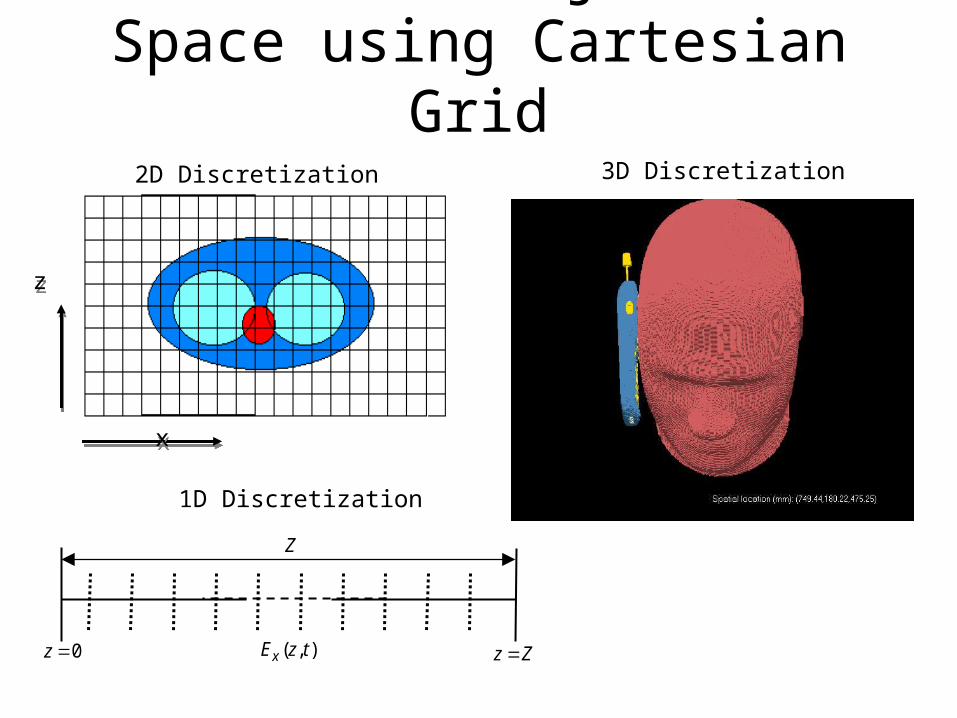
Discretize Objects in Space using Cartesian Grid

2D Discretization

Z

0z z Z( , )xE z t

1D Discretization

xx

zz

3D Discretization

Define Locations of Field Components:

FDTD Cell called Yee Cell

• Finite-Difference

– Space is divided into small cells

One Cell: (dx)(dy)(dz)

– E and H components are distributed in space around the Yee cell (note: field components are not collocated)

FDTD: Yee, K. S.: Numerical solution of initial boundary value problems involving Maxwell's equations in isotropic media. IEEE Transactions on Antennas

Propagation, Vol. AP-14, pp. 302-307, 1966.

Replace Continuous Derivatives with Differences

• Derivatives in time and space are approximated as DIFFERENCES

)(2

)('

:

'

211' hErrorh

ffxff

FormulaDifferenceCentral

curveofslopefx

f

iiii

Solution then evolves by time-marching difference equations

– Time is Discretized• One Time Step: dt

– E and H fields are distributed in time

– This is called a “leap-frog” scheme.

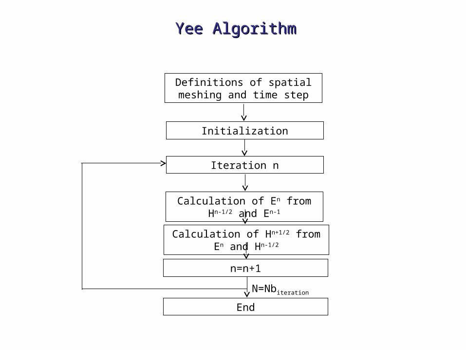
Yee AlgorithmYee Algorithm

Definitions of spatial meshing and time step

Initialization

Iteration n

Calculation of En from Hn-1/2 and En-1

Calculation of Hn+1/2 from En and Hn-1/2

n=n+1

End

N=Nbiteration

1-D FDTD

Assuming that field values can only vary in the z-direction (i.e. all spatial derivatives in x and z direction are zero),

Maxwell’s Equations reduce to:

z

E

t

Hxy

1

x

yx Ez

H

t

E

1

z

z), (z)

Ex

Hy

1-D FDTD – Staggered Grid in Space

3

2zn

xE

1

2zn

1

2zn

3

2zn

2zn 1zn zn 1zn

1

2tn

yH tn

3

2zn

xE

1

2zn

1

2zn

3

2zn 1

2tn

Time plane

Interleaving of the Ex and Hy field components in space and time in the 1-D FDTD formulation

1-D FDTD

z

E

t

Hxy

1

x

yx Ez

H

t

E

1

Replace all continuous derivatives with central finite differences

t

iEiE

t

iE nx

nx

nx

)()()( 2/12/1

t

iHiH

t

iH ny

ny

ny

)()()( 2/12/1

z

iEiE

z

iE nx

nx

nx

)2/1()2/1()(

z

iHiH

z

iH ny

ny

ny

)2/1()2/1()(

2

)()()(

2/12/1 iEiEiE

nx

nxn

x

Note: finite differences are 2nd order in time and space

1-D FDTD

Replace all continuous derivatives with finite differences

Solve for )(2/1 iE nx

x

yx Ez

H

t

E

1

t

iEiE

t

iE nx

nx

nx

)()()( 2/12/1

z

iHiH

z

iH ny

ny

ny

)2/1()2/1()(

2

)()()(

2/12/1 iEiEiE

nx

nxn

x

2

)()()2/1()2/1(1)()( 2/12/12/12/1 iEiE

z

iHiH

t

iEiE nx

nx

ny

ny

nx

nx

)2/1()2/1(2

2)(

2

2)( 2/12/1

iHiHtz

tiE

t

tiE n

yny

nx

nx

1-D FDTD

z

E

t

Hxy

1

Replace all continuous derivatives with finite differences and increment time by one half time step

t

iHiH

t

iH ny

ny

ny

)()()( 12/1

z

iEiE

z

iE nx

nx

nx

)2/1()2/1()( 2/12/12/1

z

iEiE

t

iHiH nx

nx

ny

ny )2/1()2/1(1)()( 2/12/11

Solve for )(1 iH ny

)2/1()2/1()()( 2/12/11

iEiEz

tiHiH n

xnx

ny

ny

1-D FDTD

After some simple algebra:

z

E

t

Hxy

1

x

yx Ez

H

t

E

1

)2/1()2/1()()( 2/12/11

iEiEz

tiHiH n

xnx

ny

ny

)2/1()2/1(2

2)(

2

2)( 2/12/1

iHiHtz

tiE

t

tiE n

yny

nx

nx


xE1

2tn

yH tn


i=1 i=2 i=3 i=4

z=0 z=dz z=2*dz z=3*dz

i=1 i=2 i=3 i=4

z=dz/2 z=3dz/2 z=5*dz/2 z=7*dz/2

)2/()2/()()(2

2)(

)()(2

)()(2)( 2/12/1 dzzHdzzH

ztzz

tzE

ztz

ztzzE n

yny

nx

nx

)1()()()(2

2)(

)()(2

)()(2)( 2/12/1

iHiHitiz

tiE

iti

itiiE n

yny

nx

nx


xE1

2tn

yH tn


i=1 i=2 i=3 i=4

z=0 z=dz z=2*dz z=3*dz

i=1 i=2 i=3 i=4

z=dz/2 z=3dz/2 z=5*dz/2 z=7*dz/2

)2/()2/()(

)()( 2/12/11 dzzEdzzEzz

tzHzH n

xnx

ny

ny

)()1()(

)()( 2/12/11 iEiEzi

tiHiH n

xnx

ny

ny

1-D FDTD – Basic Core of Code

)1,()1,1()(

)1,(),(

niEniE

zi

tniHniH xx

nyy

)1,1()1,()()(2

2)1,(

)()(2

)()(2),(

niHniHitiz

tniE

iti

itiniE n

yyxx

for i=2:Nx-1 % all interior nodes

end


end

for n=2:Nt % all time steps

end

Loo

p th

roug

h al

lof

the

E -

grid

Loo

p th

roug

h al

lof

the

H -

grid

Loo

p th

roug

h al

l tim

e st

eps

Note: H uses the new values of E. This isEquivalent to incrementing by ½ a time step

SOME OPEN QUESTIONS??

• How do we determine what t and z should be?• How do we implement real sources?• How do we simulate open boundaries?• How accurate is the solution?

Numerical StabilityLike all iterative algorithms FDTD has the possibility of not converging on a solution. This usually results in the algorithm going unstable and producing ever increasing field values over time. When does this happen?

222

22

111

1

11

1

zyxc

t

yxc

t

c

xt

1-D

2-D

3-D

Numerical DispersionIn real life plane waves traveling in a homogenous medium propagate at the speed of light in that medium independent of frequency or propagation direction. However, due to our approximation of continuous derivatives with finite differences if we launch a plane wave in FDTD it will actually propagate at a slightly different speed than that of light. Moreover, and more disturbing, the propagation velocity will depend on the frequency of the plane wave and its direction of propagation with respect to the FDTD grid. This effect is known as numerical dispersion. The effect has been well studied and mathematically quantified.

Numerical Dispersion

11)cos()cos(2

xkx

tct

ck

1-D FDTD

Continuous Plane Wave

ck

c

xtIIcase

ck

xtIcase

:

0,:

Magic time step!

0

2

2sin

2

2sin

2

2sin

2

2

2

22

2

22

2

22

cz

zk

y

yk

x

xk zyx

3-D FDTDAt optimal time step

t 1

c1

x 2 1

y 2 1z2

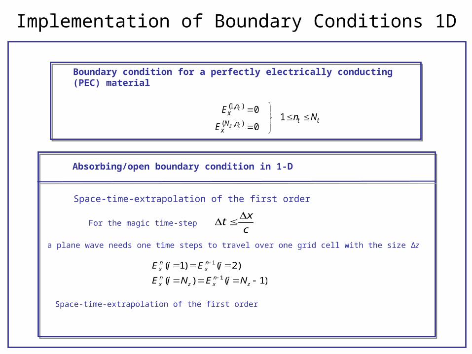
Implementation of Boundary Conditions 1D

Boundary condition for a perfectly electrically conducting (PEC) material

(1, )

( , )

01

0

t

z t

nx

t tN nx

En N

E

Absorbing/open boundary condition in 1-D

For the magic time-step

a plane wave needs one time steps to travel over one grid cell with the size ∆z

Space-time-extrapolation of the first order

Space-time-extrapolation of the first order

c

xt

E xn (i1) E x

n 1(i2)

E xn (iNz) E x

n 1(iNz 1)

(MATLAB DEMO)


direction (i.e. d/dy = 0)

zyz

xyx

xzy

Ex

H

t

E

Ez

H

t

E

z

E

x

E

t

H

1

1

1

Hx

t

1

Ey

z

Hz

t

1

Ey

x

E y

t

1

Hx

zHz

x Ey

2D - TM 2D - TE

zyz

xyx

xzy

Ex

H

t

E

Ez

H

t

E

z

E

x

E

t

H

1

1

1

2D - TM

Ex Ex

Ex Ex

Ex Ex

Ez

Ez

Ez

Ez

Ez

Ez

Hy Hy

HyHy

dz

dx

(i-1,j-1) (i,j-1) (i+1,j-1)

(i-1,j) (i,j) (i+1,j)

(i-1,j+1)(i,j+1)

(i+1,j+1)

E-GRID H-GRID

Ex Ex

Ex

Ex

Ex Ex

Ez

Ez

Ez

Ez

Ez

Ez

Hy Hy

HyHy

dz

dx

(i,j-1)

(i-1,j)

(i,j)

(i+1,j)

(i-1,j)

(i-1,j-1)

zyz

xyx

xzy

Ex

H

t

E

Ez

H

t

E

z

E

x

E

t

H

1

1

1

2D – TM: Derive FDTD EquationsEx Ex

Ex Ex

Ex Ex

Ez

Ez

Ez

Ez

Ez

Ez

Hy Hy

Hy Hydz

(i-1,j-1) (i,j-1) (i+1,j-1)

(i-1,j) (i,j) (i+1,j)

t

jiHjiH

t

jiHn

y

n

yny

),(),(),( 21

2

1

z

jiHjiH

z

jiH ny

ny

ny

)2/1,()2/1,(),(

2

),(),(),(

2/12/1 jiEjiEjiE

nx

nxn

x

t

jiEjiE

t

jiEn

x

n

xnx

),(),(),( 21

2

1

t

jiEjiE

t

jiEn

z

n

znz

),(),(),( 21

2

1

z

jiEjiE

z

jiE nx

nx

nx

)2/1,()2/1,(),(

x

jiEjiE

x

jiE nx

nx

nz

),2/1(),2/1(),(

x

jiHjiH

x

jiH ny

ny

ny

),2/1(),2/1(),(

2

),(),(),(

2/12/1 jiEjiEjiE

nz

nzn

z

(i-1,j+1) (i,,j+1) (i+1,j+1)

2D – TM: Derive FDTD Equations

z

E

x

E

t

Hxzy

1

z

jiEjiE

z

jiE nx

nx

nx

)2/1,()2/1,(),(

x

jiEjiE

x

jiE nx

nx

nz

),2/1(),2/1(),(

z

jiEjiE

x

jiEjiE

t

jiHjiH nx

nx

nz

nz

n

y

n

y )2/1,()2/1,(),2/1(),2/1(1),(),( 21

2

1

Solve for ),(2

1

jiHn

y

z

jiEjiE

x

jiEjiEtjiHjiH

nx

nx

nz

nz

n

y

n

y

)2/1,()2/1,(),2/1(),2/1(),(),( 2

1

2

1

H-GRID

Ex Ex

Ex

Ex

Ex Ex

Ez

Ez

Ez

Ez

Ez

Ez

Hy Hy

HyHy

dz

dx

(i,j-1)

(i-1,j)

(i,j)

(i+1,j)

(i-1,j)

(i-1,j-1)

2D – TM: Derive FDTD Equations

z

jiEjiE

x

jiEjiEtjiHjiH

nx

nx

nz

nz

n

y

n

y

)2/1,()2/1,(),2/1(),2/1(),(),( 2

1

2

1

z

jiHjiH

tt

jiEt

t

jiEny

nyn

xnx

)2/1,()2/1,(

21

/),(

21

21

),(2/12/1

1

x

jiHjiH

tt

jiEt

t

jiEny

nyn

znz

),2/1(),2/1(

21

/),(

21

21

),(2/12/1

1

2-D FDTD – Basic Core of Code

Hy (i, j,n) Hyn (i, j,n 1)

t(i)

E z (i 1, j,n 1) E z (i, j,n 1)

xEx (i, j 1,n 1) Ex (i, j,n 1)

z


end


end


end

Loo

p th

roug

h al

lof

the

E -

grid

Loo

p th

roug

h al

lof

the

H -

grid

Ex (i, j,n) 1

(i, j) t2(i, j)

1 (i, j) t2(i, j)

E x (i, j,n 1) t /(i, j)

1 (i, j)t2(i, j)

Hy (i, j,n 1) Hy (i, j 1,n 1)

z

E z (i, j,n) 1

(i, j) t2(i, j)

1 (i, j) t2(i, j)

E z (i, j,n 1)t /(i, j)

1 (i, j)t2(i, j)

Hy (i, j,n 1) Hy (i 1, j,n 1)

x

2D – TE: Derive FDTD Equations

Hx

n1

2 (i, j) Hx

n1

2 (i, j)t

E zn (i, j 1/2) E z

n (i, j 1/2)

z

E yn1(i, j)

1 t2

1 t2

E yn (i, j)

t /

1 t2

Hxn1/ 2(i, j 1/2) Hx

n1/ 2(i, j 1/2)

zHz

n1/ 2(i 1/2, j) Hzn1/ 2(i 1/2, j)

x

Hz

n1

2 (i, j) Hz

n1

2 (i, j) t

E yn (i 1/2, j) E y

n (i 1/2, j)

x

Using same procedure as for the 1D case we obtain:

Numerical Dispersion 2D case

)sin(~~

),cos(~~

2

~sin

1

2

~sin

1

2sin

1222

kkkk

zk

z

xk

x

t

tc

zx

zx

Source Modeling

1. We can implement a “hard” source by forcing the fields to predefined values at specific nodes in the FDTD grid.

E z (io, jo,n) Ae (nt b )2

cos(o(nt b))For example:

Source Modeling: Soft SourcesScattered Field Formulation

1. We can implement a “soft” source by first reformulating Maxwell’s equations for only the scattered field.

E tot H tot

t

H tot E tot E tot

t

E inc o

H inc

t

H inc oE inc

t

E tot E sc E inc

H tot Hsc H inc

(1) (2) (3)

(1)-(2):

(E tot E inc ) H tot

to

H inc

t

(Htot H inc ) E tot E tot

t o

E inc

t

Use (3) in aboveand a little algebra:

Hsc

t E sc ( o)

H inc

t

E sc

tHsc E sc ( o)

E inc

t E inc

Six E and H-Field EquationsScattered Field

Hxsc

t

1

Ey

sc

zE z

sc

y

o

Hx

inc

Hysc

t

1

E z

sc

xEx

sc

z

o

Hy

inc

Hzsc

t

1

Ex

sc

yEy

sc

x

o

Hz

inc

E xsc

t

1

Hz

sc

yHy

sc

z E x

sc

o

E xinc

tE x

inc

E ysc

t

1

Hx

sc

zHz

sc

x E y

sc

o

E yinc

tE y

inc

E zsc

t

1

Hy

sc

xHx

sc

y E z

sc

o

E yinc

tE y

inc

Hsc

t E sc ( o)

Hinc

t

E sc

tHsc E sc ( o)

E inc

t E inc

2DScattered Field

Hxsc

t

1

Ey

sc

z

o

Hx

inc

Hzsc

t

1

Ey

sc

x

o

Hz

inc

Eysc

t

1

Hx

sc

zHz

sc

x Ey

sc

o

Eyinc

tEy

inc

E xsc

t

1

Hy

sc

zE x

sc

o

E xinc

tE x

inc

E zsc

t

1

Hy

sc

x E z

sc

o

E yinc

tE y

inc

Hysc

t

1

E z

sc

xE x

sc

z

o

Hy

inc

t

TETM

1DScattered Field

Hxsc

t

1

E y

sc

z

o

Hx

inc

E ysc

t

1

Hx

sc

z E y

sc

o

E yinc

tE y

inc

Exsc

t

1

Hy

sc

zEx

sc

o

Exinc

tEx

inc

Hysc

t

1

Ex

sc

z

o

Hy

inc

t

TETM

1-D FDTD Scattered Fields (TE)

Hysc

t

1

Ex

sc

z

o

Hy

inc

t

E xsc

t

1

Hy

sc

zE x

sc

o

E xinc

tE x

inc

Exscn1/ 2

(i) 2 t2 t

Exscn 1/ 2

(i) 2tz 2 t

Hyscn (i 1/2) Hy

scn (i 1/2)

2t( o)2 t

Exinc

t(t (n 1/2)t, ziz)

2t2 t

Exinc (t (n 1/2)t, ziz)

Hyscn1

(i) Hyscn (i)

tz

E xscn1/ 2

(i 1/2) Exscn1/ 2

(i 1/2) t( o)

Hy

inc

t(t nt, ziz)


E xinc (z, t) Acos(ot kzz) Acos(ot

o

cz)

E xinc (z, t)

toAsin(ot

o

cz)

let

t zc

E xinc (z, t)

Acos(o ) 0

0 0

E xinc (z, t)

t Ao sin(o) 0

0 0

In FDTD

t zcnt

izc

EXAMPLE INCIDENT FIELD

1-D FDTD – Basic Core of 1D Scattered Field Code (non-magnetic)

)1,()1,1()(

)1,(),(

niEniE

zi

tniHniH xx

nyy

)1,1()1,()()(2

2)1,(

)()(2

)()(2),(

niHniHitiz

tniE

iti

itiniE n

yyxx


end


end


end

Loo

p th

roug

h al

lof

the

E -

grid

Loo

p th

roug

h al

lof

the

H -

grid

taunt izc

If tau<0

else

Ex (i,n) 2(i) t(i)2(i)t(i)

Ex (i,n 1) 2tz 2(i)t(i)

Hy (i,n 1 ) Hyn (i 1,n 1 )

2t((i) o)2(i)t (i)

Exinc

t

2t (i)

2(i)t (i) Ex

inc

end


Eyscn1/ 2

(i, j) 2 t2 t

Eyscn 1/ 2

(i, j) 2t2 t

Hxscn (i, j 1/2) Hx

sc n (i, j 1/2)

zHz

scn (i 1/2, j) Hzscn (i 1/2, j)

x

2t( o)2 t

Eyinc

t(t (n 1/2)t,x ix, z jz) 2t

2 t Ey

inc(t (n 1/2)t, x ix, z jz)

Hyscn1

(i, j) Hxscn (i, j) t

zEy

scn1/ 2(i, j 1/2) Ey

scn1/ 2(i, j 1/2)

t( o)

Hx

inc

t(t nt, x ix,z jz)

Hxsc

t

1

Ey

sc

z

o

Hx

inc

Hzsc

t

1

Ey

sc

x

o

Hz

inc

Eysc

t

1

Hx

sc

zHz

sc

x Ey

sc

o

Eyinc

tEy

inc

Hzscn1

(i, j) Hzscn (i, j)

tx

E yscn1/ 2

(i 1/2, j) E yscn1/ 2

(i 1/2, j) t( o)

Hz

inc

t(t nt, x ix,z jz)

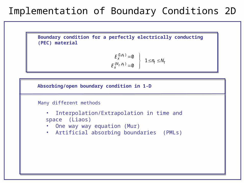
Implementation of Boundary Conditions 2D

Boundary condition for a perfectly electrically conducting (PEC) material

(1, )

( , )

01

0

t

z t

nx

t tN nx

En N

E

Absorbing/open boundary condition in 1-D

• Interpolation/Extrapolation in time and space (Liaos)• One way way equation (Mur)• Artificial absorbing boundaries (PMLs)

Many different methods

One Way Wave Equation

01

2

2

22

2

2

2

E

tcxy

2xD

2yD

2tD

0}{222 ELEDDD txy

0}{}{ ELLEL


0}{}{ ELLEL

01122

E

D

DDD

D

DDD

t

ytx

t

ytx

22

2

2

11

11

SDDD

DDDL

SDDD

DDDL

txt

ytx

txt

ytx


22

2

2

11

11

SDDD

DDDL

SDDD

DDDL

txt

ytx

txt

ytx

If we could implement the one way equations on a FDTD boundary we would have the perfect ABC (i.e. zero reflection. Unfortunately we can’t do that since we don’t know how to implement the square root operator. So we need to approximate.

11

11

2

2

S

SFirst order Taylor series expansion


txt

ytx

txt

ytx

DDD

DDDL

DDD

DDDL

2

2

1

1

01

01

2

2

Etcx

EL

Etcx

EL

Absorbing Boundary Conditions 2D: Mur 1st order

One-way Wave Equations: They approximately represent waves traveling in only one direction.

x=0 x=w

y=0

y=h

01

2

t

E

cy

E

01

2

t

E

cy

E

01

2

t

E

cx

E

01

2

t

E

cx

E

Absorbing Boundary Conditions 2D: Mur


x=0 x=wy=0

y=h

01

2

t

E

cx

E

nj

nj

nj

nj EE

xtc

xtcEE ,1

1,2,2

1,1

t

EE

t

EE

t

E

x

EE

x

EE

x

E

nj

nj

nj

nj

nj

nj

nj

nj

,21

,2,11

,1

,1,21

,11

,2

2

1

2

1

Absorbing Boundary Conditions 2D: 1st Order Mur

2D 1st Order Mur Equation

x=0 x=wy=0

y=h

nj

nj

nj

nj EE

xtc

xtcEE ,1

1,2,2

1,1

nNyi

nNyi

nNyi

nNyi EE

ytc

ytcEE ,

11,1,

1,

njNx

njNx

njNx

njNx EE

xtc

xtcEE ,

1,1,1

1,

ni

ni

ni

ni EE

ytc

ytcEE 1,

12,2,

11,

Absorbing Boundary Conditions 2D: Mur 2nd Order


x=0 x=wy=0

y=h

2E

yt

1

c

2E

t 2c

2

2E

x 20

2E

yt

1

2tE n1

xE n 1

x

1

2tE i,Ny

n1 E i,Ny 1n1

yE i,Ny

n 1 E i,Ny 1n 1

y

2E

t 2

1

2

2E i,Nyn

t 22E i,Ny 1

n

t 2

1

2

E i,Nyn1 2E i,Ny

n E i,Nyn 1

t 2E i,Ny 1

n1 2E i,Ny 1n E i,Ny 1

n 1

t 2

2E

x 2

1

2

2E i,Nyn

x 22E i,Ny 1

n

x 2

1

2

E i1,Nyn 2E i,Ny

n E i 1,Nyn

x 2E i1,Ny 1

n 2E i,Ny 1n E i 1,Ny 1

n

x 2

(MATLAB DEMO)

Finite Difference Time Domain Method (FDTD). FDTD: The Basic Algorithm Maxwell’s Equations in the...

Documents

Transcript of Finite Difference Time Domain Method (FDTD). FDTD: The Basic Algorithm Maxwell’s Equations in the...