Finding Motifs in DNA

References:1. Bioinformatics Algorithms, Jones and Pevzner, Chapter 4.2. Algorithms on Strings, Gusfield, Section 7.11.3. Beginning Perl for Bioinformatics, Tisdall, Chapter 9.4. Wikipedia

Summary

• Introduce the Motif Finding Problem

• Explain its significance in bioinformatics

• Develop a simple model of the problem

• Design algorithmic solutions:– Brute Force– Branch and Bound– Greedy

• Compare results of each method.

News: October 6, 2009

IBM Developing Chip to Sequence DNA3 Scientists Share Nobel Chemistry Prize for DNA Work

DNA on bloody clothes matches missing US diplomat

Gene Discovery May Advance Head and Neck Cancer Therapy

Updated map of human genome to help fight against disease

Need a New Heart? Grow Your OwnS1P Gene Regulating Lipid May Help Develop New Drugs against Cancer

DNA DNA DNA

The Motif Finding Problem

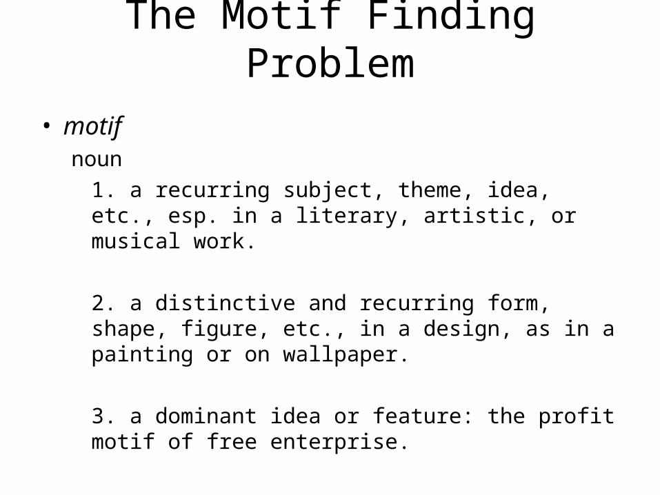
• motifnoun

1. a recurring subject, theme, idea, etc., esp. in a literary, artistic, or musical work.

2. a distinctive and recurring form, shape, figure, etc., in a design, as in a painting or on wallpaper.

3. a dominant idea or feature: the profit motif of free enterprise.

Example: Fruit Fly

• Set of immunity genes.• DNA pattern:

TCGGGGATTTCC• Consistently appears upstream

of this set of genes.• Regulates timing/magnitude of

gene expression.• “Regulatory Motif”• Finding such patterns can be

difficult.

Construct an Example:

7 DNA Samplescacgtgaagcgactagctgtactattctgcatcgtccgatctcaggattgtctggggcgacgatgggggcggtgcgggagccagcgctcggcgtttgcaaggcgtcaaattgggaggcgcattctgaaccacaagcgagcgttcctcgggattggtcacgaggtataatgcgaacagctaaaactccggaaacccccgcaatttaactagggggcgcttagcgt

Patternacctggcc

Insert Pattern at random locations:

cacgtgaacctggccagcgactagctgtactattctgcatcgtccgatctcaggattgtctacctggccggggcgacgatgacctggccggggcggtgcgggagccagcgctcggcgtttgcaaggacctggcccgtcaaattgggaggcgcattctgaaccacaagcgagcgttcctcgggattggacctggcctcacgaggtataatgcgaaacctggcccagctaaaactccggaaacccccgcaaacctggcctttaactagggggcgcttagcgt

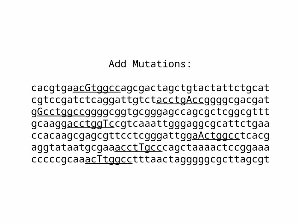
Add Mutations:

cacgtgaacGtggccagcgactagctgtactattctgcatcgtccgatctcaggattgtctacctgAccggggcgacgatgGcctggccggggcggtgcgggagccagcgctcggcgtttgcaaggacctggTccgtcaaattgggaggcgcattctgaaccacaagcgagcgttcctcgggattggaActggcctcacgaggtataatgcgaaacctTgcccagctaaaactccggaaacccccgcaaacTtggcctttaactagggggcgcttagcgt

Finally, find the hidden pattern:

cacgtgaacgtggccagcgactagctgtactattctgcatcgtccgatctcaggattgtctacctgaccggggcgacgatggcctggccggggcggtgcgggagccagcgctcggcgtttgcaaggacctggtccgtcaaattgggaggcgcattctgaaccacaagcgagcgttcctcgggattggaactggcctcacgaggtataatgcgaaaccttgcccagctaaaactccggaaacccccgcaaacttggcctttaactagggggcgcttagcgt

cacgtgaacgtggccagcgactagctgtactattctgcatcgtccgatctcaggattgtctacctgaccggggcgacgatggcctggccggggcggtgcgggagccagcgctcggcgtttgcaaggacctggtccgtcaaattgggaggcgcattctgaaccacaagcgagcgttcctcgggattggaactggcctcacgaggtataatgcgaaaccttgcccagctaaaactccggaaacccccgcaaacttggcctttaactagggggcgcttagcgt

Three Approachs

• Brute Force:– check every possible pattern.

• Branch and Bound: – prune away some of the search space.

• Greedy: – commit to “nearby” options, never look back.

Brute Force

• Given that the pattern is of length = L.

• Generate all DNA patterns of length L.

• (Called “L-mers”).

• Match each one to the DNA samples.

• Keep the L-mer with the best match.

• “Best” is Based on a scoring function.

Scoring: Hamming Distance

accgtaccggtaacaagtaccgtacgggtaacaagtaccgtaggtgtaacaagt

gtgtaggt

4 mismatches

gtgtaggt

2 mismatches

gtgtaggt

8 mismatches

dna sequence

Try all starting positions

Find the position with the fewest mismatches

L=8 gtgtaggtan L-mer

Scoring

t = 8 DNA samples

try all possible L-mers

Try each possible L-mer

Score is equal to the sum of the mismatches at the locations with

fewest mismatches on each string.

The L-mer with the lowest such

score is the optimal answer.

32103201

total distance = 12

12

Generating all L-mers

• Systematic enumeration of all DNA strings of length L.

• DNA has an “alphabet” of 4 letters:{ a, c, g, t }

• Proteins have an alphabet of 20 letters:– one for each of 20 possible amino acids.– {A,B,C,D,E,F,G,H,I,K,L,M,N,P,Q,R,S,T,V,W}

• Solve problem for any size alphabet (k) and any size L-mer (L).

Definitions

• k = size of alphabet

• L = length of strings to be generated

• a = vector containing a partial or complete L-mer.

• i = number of entries in a already filled in.

• Example:k = 4, L = 5, i = 2, a = (2, 4, *, * , * )

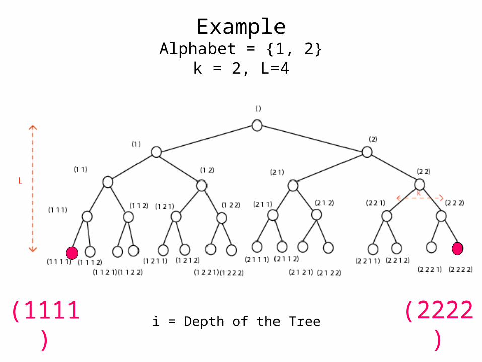
ExampleAlphabet = {1, 2}

k = 2, L=4

i = Depth of the Tree(1111) (2222)

NEXT VERTEXi = 3 a = 1 3 2

i = 4 a = 1 3 2 1

1

i = L a = 2 3 2 1 2 2

j = Lj = 1i = L a = 2 3 2 1 2 3

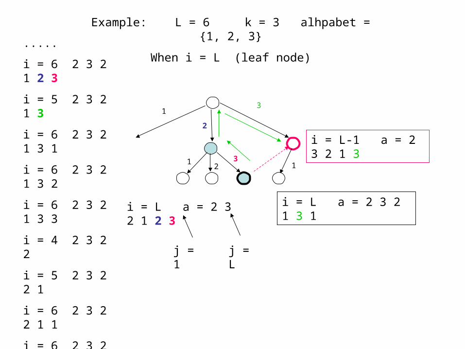
NEXTVERTEX(a, i, L, k)if i < L

a(i+1) = 1return (a, i+1)

elsefor j = L to j = 1

if a(j) < k then a(j) = a(j) +1 return(a, j)

return (a,0)

i = L a = 2 3 2 1 2 3

j = Lj = 1

12

3

2

13

i = L-1 a = 2 3 2 1 3

1

i = L a = 2 3 2 1 3 1

.....

i = 6 2 3 2 1 2 3

i = 5 2 3 2 1 3

i = 6 2 3 2 1 3 1

i = 6 2 3 2 1 3 2

i = 6 2 3 2 1 3 3

i = 4 2 3 2 2

i = 5 2 3 2 2 1

i = 6 2 3 2 2 1 1

i = 6 2 3 2 2 1 2

i = 6 2 3 2 2 1 3

.....

Example: L = 6 k = 3 alhpabet = {1, 2, 3}

When i = L (leaf node)

Brute Force

• Use NEXTVERTEX to generate nodes in the tree.

• Translate each numeric value into the corresponding L-mer – (e.g.: 1=a, 2=c, 3=g, 4=t).

• Score each L-mer (Hamming distance).

• keep the best L-mer (and where it matched in each dna sample).

Branch and Bound

• Use same structure as the Brute Force method.

• Looks for ways to reduce the computation.

• Prune branches of the tree that cannot produce anything better than what we have so far.

BYPASS

• BYPASS (a, i, L, k)

• for j = i to j = 1– if a(j) < k

• a(j) = a(j) + 1• return (a, j)

• return (a, 0)

BRANCHANDBOUND

• a = (1, 1, ..., 1)• bestDistance = infinity• i = L• while (i > 0)

– if i < L• prefix = translate(a1, a2, ..., ai)• optimisticDistance = TotalDistance(prefix)• if optimisticDistance > bestDistance

– (a, i) = BYPASS(a, i)• else

– (a, i) = NEXTVERTEX( a, i )

– else• word = translate (a1, a2, ....., aL)• if TotalDistance( word, DNA ) < bestDistance

– bestDistance = TotalDistance(word, DNA) – bestWord = word

• (a, i) = NEXTVERTEX( a, i)• return bestWord

Greedy Method

• Picks a “good” solution.

• Avoids backtracking.

• Can give good results.

• Generally, not the best possible solution.

• But: FAST.

Greedy Method

• Given t dna samples (each n-long).• Find the optimal motif for the first two samples.• Lock that choice in place.• For the remainder of the samples:

– for each dna sample in turn• find the L-mer that best fits with the prior choices.• never backtrack.

t = 8 DNA samples

Step 1: Grab the first two samples and find the optimal alignment

(consider all starting points s1 and s2, and keep the largest score).

Step 2: Go through each remaining sample, successively finding the starting positions (s3, s4, ...., st) that give the best consensus

score for all the choices made so far.

a t c c a g c t

g g g c a a c t

a t g g a t c t

a a g c a a c c

t t g g a a c t

3 1 0 0 5 3 0 0

1 3 0 0 0 1 0 4

1 1 4 2 0 1 0 0

0 0 1 3 0 0 5 1

a

t

g

c

3 3 4 3 5 3 5 4

Consensus

Profile

Alignment

a g g c a a c tScoring

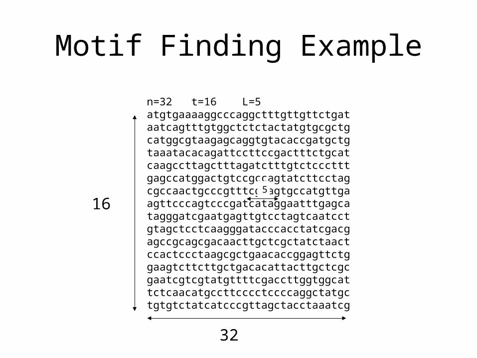
Motif Finding Example

n=32 t=16 L=5atgtgaaaaggcccaggctttgttgttctgataatcagtttgtggctctctactatgtgcgctgcatggcgtaagagcaggtgtacaccgatgctgtaaatacacagattccttccgactttctgcatcaagccttagctttagatctttgtctccctttgagccatggactgtccgccagtatcttcctagcgccaactgcccgtttcgcagtgccatgttgaagttcccagtcccgatcataggaatttgagcatagggatcgaatgagttgtcctagtcaatcctgtagctcctcaagggatacccacctatcgacgagccgcagcgacaacttgctcgctatctaactccactccctaagcgctgaacaccggagttctggaagtcttcttgctgacacattacttgctcgcgaatcgtcgtatgttttcgaccttggtggcattctcaacatgccttcccctccccaggctatgctgtgtctatcatcccgttagctacctaaatcg

16

32

5

atgtgaaaaggcccaggctttgttgttctgat *****aatcagtttgtggctctctactatgtgcgctg *****catggcgtaagagcaggtgtacaccgatgctg *****taaatacacagattccttccgactttctgcat *****caagccttagctttagatctttgtctcccttt *****gagccatggactgtccgccagtatcttcctag *****cgccaactgcccgtttcgcagtgccatgttga *****agttcccagtcccgatcataggaatttgagca *****tagggatcgaatgagttgtcctagtcaatcct *****gtagctcctcaagggatacccacctatcgacg *****agccgcagcgacaacttgctcgctatctaact *****ccactccctaagcgctgaacaccggagttctg *****gaagtcttcttgctgacacattacttgctcgc *****gaatcgtcgtatgttttcgaccttggtggcat *****tctcaacatgccttcccctccccaggctatgc *****tgtgtctatcatcccgttagctacctaaatcg *****

atgtgaaaaggcccaggctttgttgttctgat*****aatcagtttgtggctctctactatgtgcgctg *****catggcgtaagagcaggtgtacaccgatgctg *****taaatacacagattccttccgactttctgcat *****caagccttagctttagatctttgtctcccttt *****gagccatggactgtccgccagtatcttcctag *****cgccaactgcccgtttcgcagtgccatgttga *****agttcccagtcccgatcataggaatttgagca *****tagggatcgaatgagttgtcctagtcaatcct *****gtagctcctcaagggatacccacctatcgacg *****agccgcagcgacaacttgctcgctatctaact *****ccactccctaagcgctgaacaccggagttctg *****gaagtcttcttgctgacacattacttgctcgc *****gaatcgtcgtatgttttcgaccttggtggcat *****tctcaacatgccttcccctccccaggctatgc *****tgtgtctatcatcccgttagctacctaaatcg *****

consensus_string = ctcccconsensus_count = 12 13 12 13 13final percent score = 78.75

consensus_string = atgtgconsensus_count = 14 10 11 12 10final percent score = 71.25

Branch and Bound Greedy

ggcccctctccaccgcttccctccccttccctgccttcccgtcctctcctctcgcctcccctcgccgaccctcccatccc

consensus_string = ctccccount = 12 13 12 13 13

final percent score = 78.75

atgtgatgtgaggtgttctgatcttatggaatgttatttgatgagaagggacttgaagcgaagtcatgttacatggtgtc

consensus_string = atgtgcount = 14 10 11 12 10

final percent score = 71.25

Branch and Bound Greedy

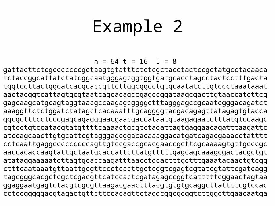
Example 2

n = 64 t = 16 L = 8gattacttctcgcccccccgctaagtgtatttctctcgctacctactccgctatgcctacaacatctaccggcattatctatcggcaatgggagcggtggtgatgcacctagcctactcctttgactatggtccttactggcatcacgcaccgttcttggcggcctgtgcaatatcttgtccctaaataaataactacggtcattagtgcgtaatcagcacagccgagccggataagcgacttgtaaccatcttcggagcaagcatgcagtaggtaacgccaagagcggggctttagggagccgcaatcgggacagatctaaaggttctctggatctatagctcacaaatttgcaggggtacgacagagttatagagtgtaccaggcgctttcctcccgagcagagggaacgaacgaccataatgtaagagaatctttatgtccaagccgtcctgtccatacgtatgttttcaaaactgcgtctagattagtgaggaacagatttaagattcatccagcaacttgtgcattcgtagggagcggacacaaaggacatgatcagacgaaacctattttcctcaattgaggcccccccccagttgtccgaccgcacgaaccgcttcgcaaaagtgttgcccgcaaccacaccaagtattgctaatgcaccattcttatgtttttgagcagcaaagcgactacgctgtatataggaaaaatcttagtgcaccaagatttaacctgcactttgctttgaaatacaactgtcggctttcaataaatgttaattgcgttccctcacttgctcggtcgagtcgtatcgtattcgatcaggtagcgggcacgctcgctcgacgttcatccactcgatagagccggtcatttttcggaactagtaaggaggaatgagtctacgtcgcgttaagacgaactttacgtgtgtgcaggcttattttcgtccaccctccgggggacgtagactgttcttccacagttctaggcggcgcggtcttggcttgaacaatga

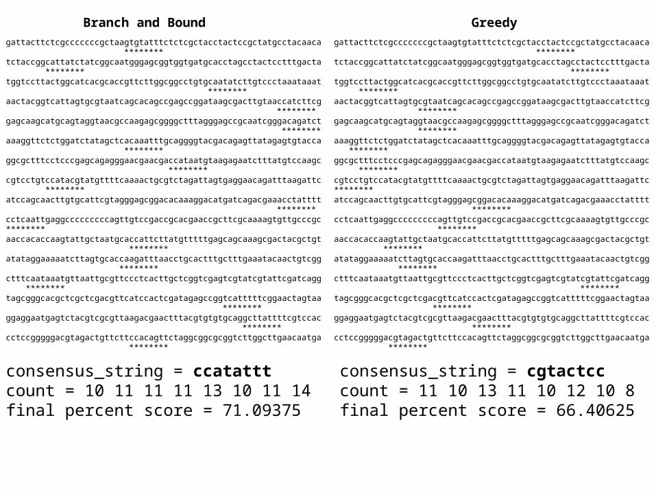
gattacttctcgcccccccgctaagtgtatttctctcgctacctactccgctatgcctacaaca ********tctaccggcattatctatcggcaatgggagcggtggtgatgcacctagcctactcctttgacta ********tggtccttactggcatcacgcaccgttcttggcggcctgtgcaatatcttgtccctaaataaat ********aactacggtcattagtgcgtaatcagcacagccgagccggataagcgacttgtaaccatcttcg ********gagcaagcatgcagtaggtaacgccaagagcggggctttagggagccgcaatcgggacagatct ********aaaggttctctggatctatagctcacaaatttgcaggggtacgacagagttatagagtgtacca ********ggcgctttcctcccgagcagagggaacgaacgaccataatgtaagagaatctttatgtccaagc ********cgtcctgtccatacgtatgttttcaaaactgcgtctagattagtgaggaacagatttaagattc ********atccagcaacttgtgcattcgtagggagcggacacaaaggacatgatcagacgaaacctatttt ********cctcaattgaggcccccccccagttgtccgaccgcacgaaccgcttcgcaaaagtgttgcccgc********aaccacaccaagtattgctaatgcaccattcttatgtttttgagcagcaaagcgactacgctgt ********atataggaaaaatcttagtgcaccaagatttaacctgcactttgctttgaaatacaactgtcgg ********ctttcaataaatgttaattgcgttccctcacttgctcggtcgagtcgtatcgtattcgatcagg ********tagcgggcacgctcgctcgacgttcatccactcgatagagccggtcatttttcggaactagtaa ********ggaggaatgagtctacgtcgcgttaagacgaactttacgtgtgtgcaggcttattttcgtccac ********cctccgggggacgtagactgttcttccacagttctaggcggcgcggtcttggcttgaacaatga ********

gattacttctcgcccccccgctaagtgtatttctctcgctacctactccgctatgcctacaaca ********tctaccggcattatctatcggcaatgggagcggtggtgatgcacctagcctactcctttgacta ********tggtccttactggcatcacgcaccgttcttggcggcctgtgcaatatcttgtccctaaataaat ********aactacggtcattagtgcgtaatcagcacagccgagccggataagcgacttgtaaccatcttcg ********gagcaagcatgcagtaggtaacgccaagagcggggctttagggagccgcaatcgggacagatct ********aaaggttctctggatctatagctcacaaatttgcaggggtacgacagagttatagagtgtacca ********ggcgctttcctcccgagcagagggaacgaacgaccataatgtaagagaatctttatgtccaagc ********cgtcctgtccatacgtatgttttcaaaactgcgtctagattagtgaggaacagatttaagattc********atccagcaacttgtgcattcgtagggagcggacacaaaggacatgatcagacgaaacctatttt ********cctcaattgaggcccccccccagttgtccgaccgcacgaaccgcttcgcaaaagtgttgcccgc ********aaccacaccaagtattgctaatgcaccattcttatgtttttgagcagcaaagcgactacgctgt ********atataggaaaaatcttagtgcaccaagatttaacctgcactttgctttgaaatacaactgtcgg ********ctttcaataaatgttaattgcgttccctcacttgctcggtcgagtcgtatcgtattcgatcagg ********tagcgggcacgctcgctcgacgttcatccactcgatagagccggtcatttttcggaactagtaa ********ggaggaatgagtctacgtcgcgttaagacgaactttacgtgtgtgcaggcttattttcgtccac ********cctccgggggacgtagactgttcttccacagttctaggcggcgcggtcttggcttgaacaatga ********

consensus_string = ccatatttcount = 10 11 11 11 13 10 11 14final percent score = 71.09375

consensus_string = cgtactcccount = 11 10 13 11 10 12 10 8final percent score = 66.40625

Branch and Bound Greedy

Summary

• Introduce the Motif Finding Problem

• Explain its significance in bioinformatics

• Develop a simple model of the problem

• Design algorithmic solutions:– Brute Force– Branch and Bound– Greedy

• Compare results of each method.

Teaching and Learning

Neural Networks for

OptimizationBill Wolfe

California State University Channel Islands

Reference

A Fuzzy Hopfield-Tank TSP Model Wolfe, W. J. INFORMS Journal on Computing, Vol. 11, No. 4, Fall 1999 pp. 329-344

Neural Models

• Simple processing units• Lots of them• Highly interconnected• Exchange excitatory and inhibitory signals• Variety of connection architectures/strengths• “Learning”: changes in connection strengths• “Knowledge”: connection architecture• No central processor: distributed processing

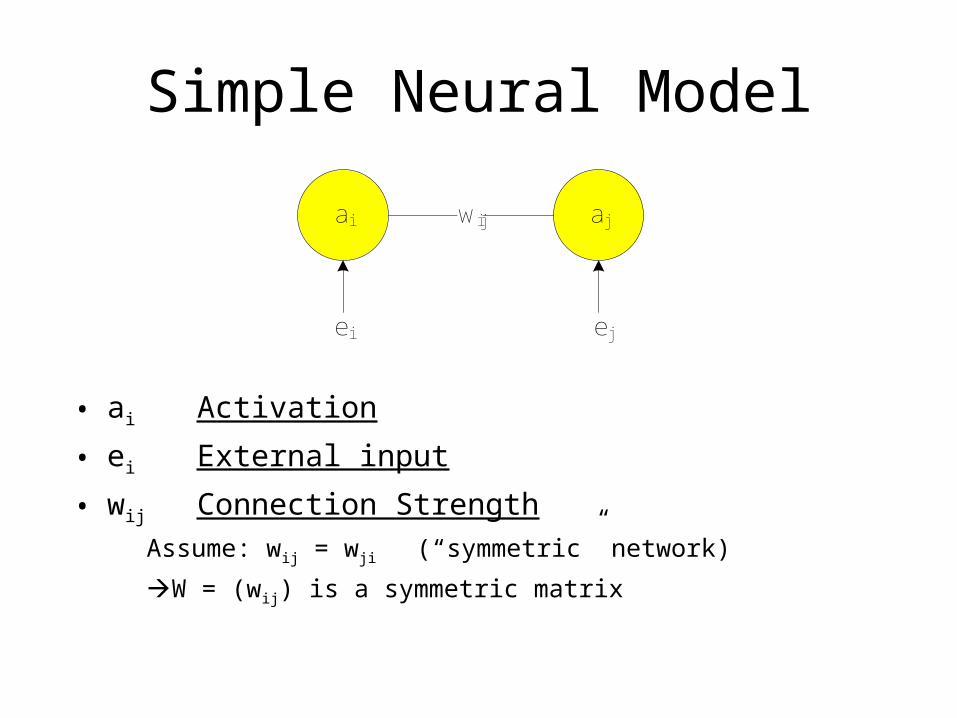
Simple Neural Model

• ai Activation

• ei External input

• wij Connection Strength

Assume: wij = wji (“symmetric” network)

W = (wij) is a symmetric matrix

ai ajwij

ei ej

Net Input

eaWnet

i

j

jiji eawnet ai

aj

wij

Vector Format:

Dynamics

• Basic idea:

ai

neti > 0

ai

neti < 0

ii

ii

anet

anet

0

0

netdt

adnet

dt

dai

i

Energy

aeaWaE TT 21

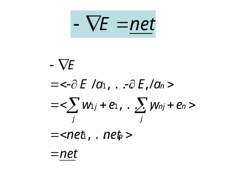
net

netnet

ewew

aEaE

E

n

j

nnj

j

j

n

,...,

,...,

/,....,/

1

11

1

netE

Lower Energy

• da/dt = net = -grad(E) seeks lower energy

net

Energy

a

Problem: Divergence

Energy

net a

A Fix: Saturation

))(1( iiii

aanetdt

da

corner-seeking

lower energy

10 ia

Keeps the activation vector inside the hypercube boundaries

a

Energy

0 1

))(1( iiii

aanetdt

da

corner-seeking

lower energy

Encourages convergence to corners

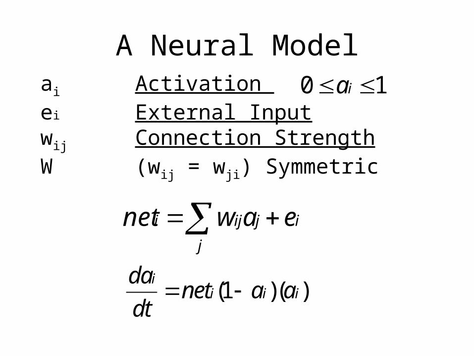
A Neural Model

))(1( iiii

aanetdt

da

i

j

jiji eawnet

ai Activation ei External Inputwij Connection StrengthW (wij = wji) Symmetric

10 ia

Example: Inhibitory Networks

• Completely inhibitory– wij = -1 for all i,j– winner take all

• Inhibitory Grid– neighborhood inhibition– on-center, off-surround

Traveling Salesman Problem

• Classic combinatorial optimization problem

• Find the shortest “tour” through n cities

• n!/2n distinct tours

D

D

AE

B

C

AE

B

C

ABCED

ABECDD

D

AE

B

C

AE

B

C

ABCED

ABECD

TSP solution for 15,000 cities in Germany

Ref: http://www.math.cornell.edu/~durrett/probrep/probrep.html

TSP

50 City Example

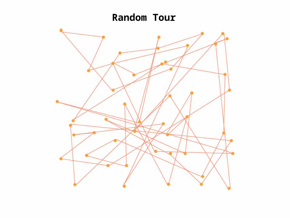
Random Tour

Nearest-City Tour

2-OPT Tour

Centroid Tour

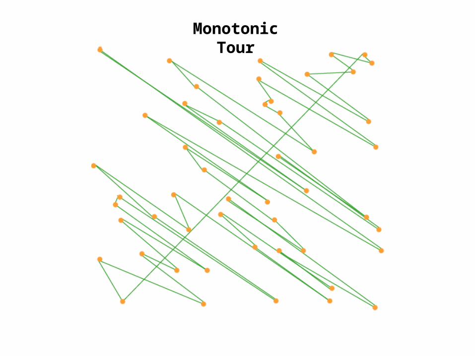
Monotonic Tour

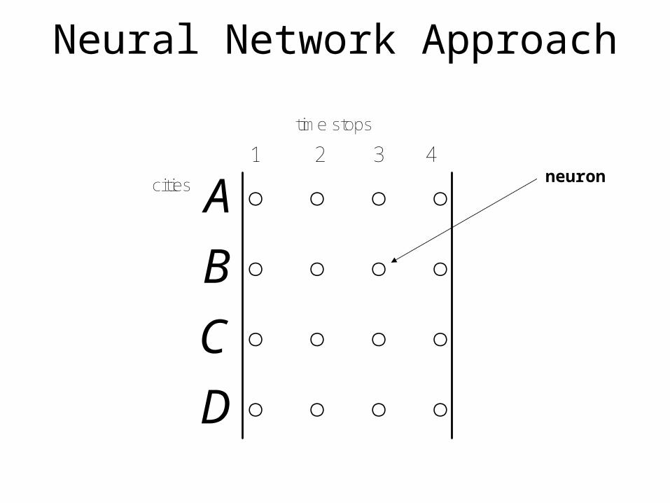
Neural Network Approach

D

C

B

A1 2 3 4

time stops

cities neuron

Tours – Permutation Matrices

D

C

B

A

tour: CDBA

permutation matrices correspond to the “feasible” states.

Not Allowed

D

C

B

A

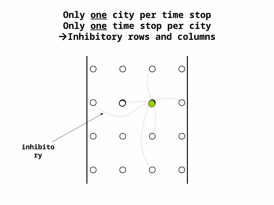
Only one city per time stopOnly one time stop per city

Inhibitory rows and columns

inhibitory

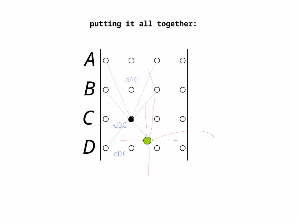
Distance Connections:

Inhibit the neighboring cities in proportion to their distances.

D

C

B

A-dAC

-dBC

-dDC

D

A

B

C

D

C

B

A-dAC

-dBC

-dDC

putting it all together:

E = -1/2 { ∑i ∑x ∑j ∑y aix ajy wixjy }

= -1/2 {

∑i ∑x ∑y (- d(x,y)) aix ( ai+1 y + ai-1 y) + ∑i ∑x ∑j (-1/n) aix ajx + ∑i ∑x ∑y (-1/n) aix aiy +

∑i ∑x ∑j ∑y (1/n2) aix ajy

}

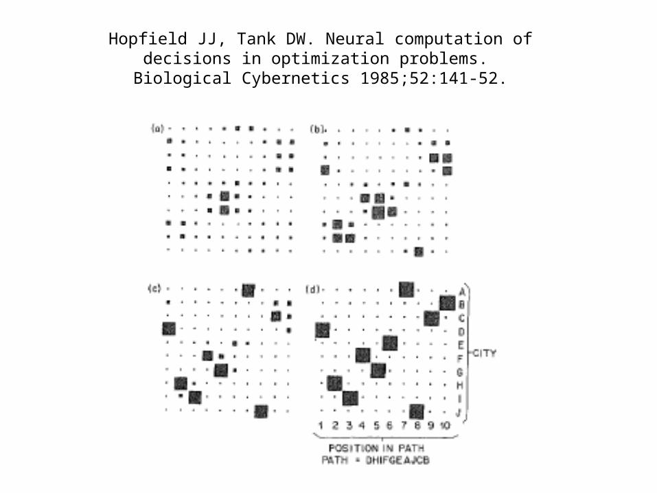
Hopfield JJ, Tank DW. Neural computation of decisions in optimization problems.

Biological Cybernetics 1985;52:141-52.

A

B

C

D

E

F

G

1 2 3 4 5 6 7

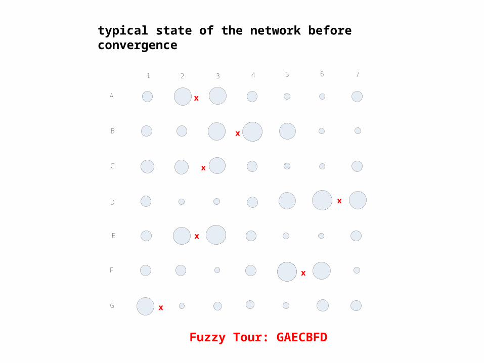
typical state of the network before convergence

x

x

x

x

x

x

x

Fuzzy Tour: GAECBFD

“Fuzzy Readout”

A

B

C

D

E

F

G

1 2 3 4 5 6 7

à GAECBFD

A

B

C

D

E

F

G

24

23

22

21

20

19

18

17

16

15

14

13

12

11

10

9

8

7

6

to

ur

len

gt

h

10009008007006005004003002001000iteration

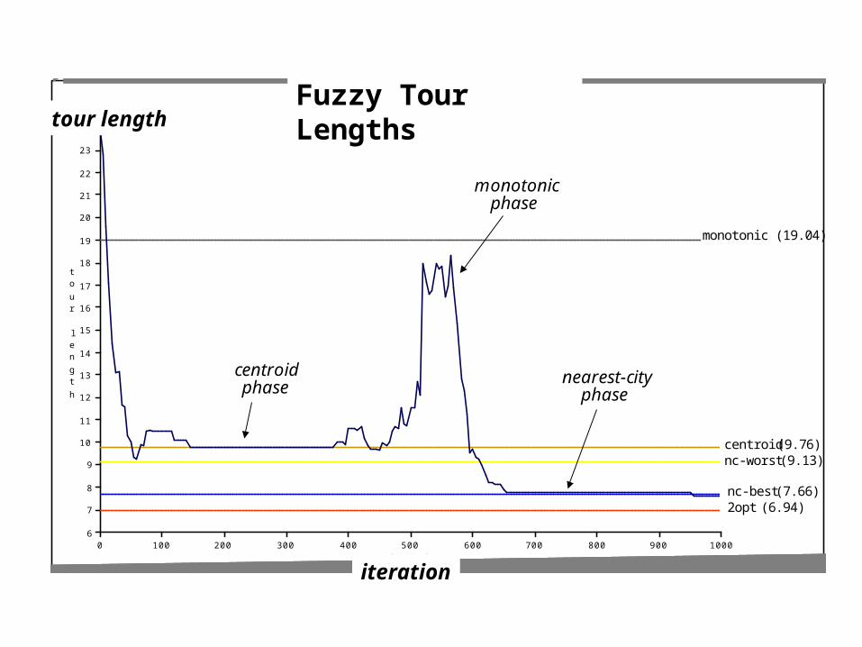
Fuzzy Tour Lengths

centroidphase

monotonicphase

nearest-cityphase

monotonic (19.04)

centroid (9.76)nc-worst (9.13)

nc-best (7.66)2opt (6.94)

Fuzzy Tour Lengthstour length

iteration

12

11

10

9

8

7

6

5

4

3

2

tour length

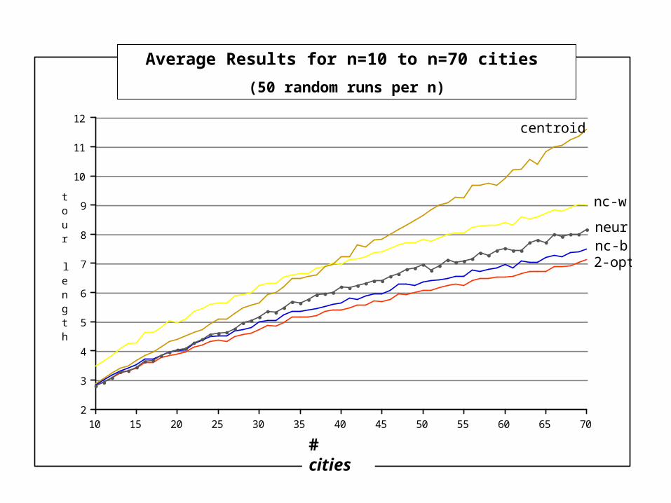
70656055504540353025201510# cities

average of 50 runs per problem size

centroid

nc-w

nc-bneur

2-opt

Average Results for n=10 to n=70 cities

(50 random runs per n)

# cities

Conclusions

• Neurons stimulate intriguing computational models.

• The models are complex, nonlinear, and difficult to analyze.

• The interaction of many simple processing units is difficult to visualize.

• The Neural Model for the TSP mimics some of the properties of the nearest-city heuristic.

• Much work to be done to understand these models.