
Financialization and Commodity - Princeton University · · 2016-03-28Financialization and...
71
Financialization and Commodity Markets 1 V. V. Chari, University of Minnesota Lawrence J. Christiano, Northwestern University 1 Research supported by Global Markets Institute at Goldman Sachs.
Transcript of Financialization and Commodity - Princeton University · · 2016-03-28Financialization and...

Financialization and CommodityMarkets1
V. V. Chari, University of MinnesotaLawrence J. Christiano, Northwestern University
1Research supported by Global Markets Institute at Goldman Sachs.

Observations• Commodity prices
— since 2000, trend and volatility appear to have changed.
Monthly Data1990 2000 2010
0.45
0.5
0.55
0.6
0.65
0.7
Figure: log(Producer Price Index: All Commodities/PCEPI)
• Trade in commodity futures markets.— since 2000, volume of trade has increased substantially.

Question
• What is the empirical link between financialization and thebehavior of commodity prices?
— Time series at best only suggestive because it consists of oneobservation.
— Cross-sectional evidence may be more informative.

Empirical Method
• Use information on a cross-section of commodities.— Construct and study a panel dataset with 131 commoditiesover 20 years.
— Huge variation in futures markets across commodities• Many commodities not traded at all in futures markets.• Among traded commodities, much variation in trade volume.
• Advantage of studying cross-section: can potentially distinguishbetween
— Was the change in price behavior a consequence of theincreased volume in futures markets?
— Or, was it a consequence of other factors (‘growth in China?’)that affected all commodities?

Answers• What is the empirical link between changes in spot pricebehavior and changes in volume of trade?— No systematic association.
• Do traded (i.e, more financialized) commodities exhibit higherprice volatility than non-traded commodities?— Traded commodities exhibit modestly less volatility.
• But, literature shows that trade volume does matter for futuresreturns (Hong-Yogo).— How can trade volume matter for futures prices but not spotprices?
• Can theory account for all these observations?— Yes.— A classic theory can account for these observations.

Literature and Our Contribution• Substantial disagreement in the literature
— Financialization does not matter: Hamilton and Wu (2012),Irwin and Sanders (2011), Killian and Murphy (2013).
— Financialization does matter: Buyuksahin and Robe (2013),Hong and Yogo (2012), Tang and Xiong (2012).• Evidence of market segmentation: Acharya et al (2011) andEtula (2010)
• Literature only looks at traded commodities.— typically uses only a small subset of traded commodities.— each paper uses different measures of financialization anddifferent methods for measuring its impact.
• Our contribution:— construct a panel dataset of prices, quantities and measures offinancialization• 131 traded and non-traded commodities over 20 years
— use variation over time series and cross section to investigateimportance of financialization.

Measuring Financialization
• Notation for futures markets:
SL : number of long positions (e.g., ‘bushels of wheat’)held by non-commercial traders (‘outsiders’)
Ss : number of short positions of outsidersHL : number of long positions
held by commercial traders (‘insiders’)
Hs : number of short positions held by insiders
• Data from CFTC on all trades in organized futures exchangesin the United States
• Would like to have data on over-the-counter and overseasmarkets.
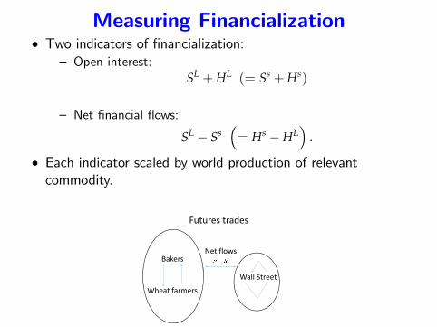
Measuring Financialization• Two indicators of financialization:
— Open interest:SL +HL (= Ss +Hs)
— Net financial flows:
SL − Ss(= Hs −HL
).
• Each indicator scaled by world production of relevantcommodity.
Futures trades
Bakers
Wheat farmers
Wall Street
Net flows

Index Construction• Construct aggregate index of prices and financialization.
— Each commodity price is divided by GDP deflator.
Pt =131
∑i=1
wiPit, Pi,t: ith commodity price/GDP deflator
wi =1T ∑
t
(PitYi,t
∑j PjtYj,t
).
• Also compute aggregate indices of financialization in the sameway:
oit =28
∑i=1
wiSL
i,t +HLi,t
Yi,t, nfft =
28
∑i=1
wiSL
i,t − Ssi,t
Yi,t, wi =
wi
∑28j=1 wj
Yi,t : world production of commodity i in year t

Data Sources
• CFTC— Volume of trade on all commodity futures contracts onorganized exchanges in the US.
— For each CFTC commodity, we identify measure of worldproduction
• Some issues: HOGS in CFTC matched with ‘pig crop’, ‘PORKBELLIES’with ‘pig crop’.
• Indices of World Production and Prices.— Fuels: British Petroleum website.— Minerals: US Geological Survey.— Food and softs: Food and Agriculture Organization of UnitedNations (FAOSTAT)
• Some cases, do not have price indices for world production, soused US price.

Commodity Price Index Behavior• Our commodity price index behaves similarly to the BLS’sProducer Price Index:
−0.074
−0.019
0.036
0.091
0.146
log,
rea
l spo
t pric
eFigure 1: Broad Indicators of Commodity Prices
19921993
19951997
19992001
20032005
20072009
−0.3
−0.087
0.125
0.338
0.55
log,
rea
l spo
t pric
e
Producer Price Index: All Commodities (left scale)
Our constructed commodity index (right scale)

Financialization Behavior• Indices of open interest and net flows
— open interest jumped from on average one-half of worldproduction to 2.5 times world production.
— net financial flows rose only a tiny bit.
1992 1994 1996 1998 2000 2002 2004 2006 2008 2010−0.5
0
0.5
1
1.5
2
2.5
3
ratio
Figure 2: Indices of Commodity Trade Volume
Open Interest
Net Financial Flows

Source of Increase in Open Interest
• Most of the higher volume is increased intra-group trade withinoutsiders and within insiders.
∆SL
∆oi = 0.27 ∆HL
∆oi = 0.73
• Outsiders’share of open interest is growing, but it’s small
1992 2009SL
oi 0.12 0.24

Motivation for Analyzing IndividualCommodities
• Consider some statistic of prices (e.g., volatility), yi, and somestatistic of financialization (e.g., open interest), xi, in 2 periods.
• Suppose∆yi = β∆xi + ∆d+ ∆εi,
where ∆d is a common shock (e.g., d ~‘Growth in China’).— Consider aggregate relation:
∆y = β∆x+ ∆d+ ∆ε, y =1n
n
∑i=1
yi, etc.
— Problem: cannot uncover β with only one observation.
• Data at level of individual commodities potentially informative.— Regression of ∆yi on ∆xi : if εi ⊥ ∆xi, slope is β and ∆dabsorbed in constant term.
Outline
• Impact of financialization on:— Dynamics of spot prices.— Dynamics of futures returns.
• Interpret the results in the light of a model.

Analysis of Commodity Spot PriceDynamics and Financialization
• Two approaches.
• ‘Structural Break’approach.
• ‘Centered Moving Average’approach.

Comparisons of Means and StandardDeviations
• Mean of mean ∆ log P in post- and pre- 2000s: X and Y
X− YsX−Y
, sX−Y =
√s2
1T1+
s22
T2.
— Used ‘large N, small T’asymptotic theory from Ibragimov andMüller, (2010, 2011), tr, where r is degrees of freedomadjustment that allows for possible change in standarddeviation across samples.
— Also, used a bootstrap procedure to compute p−values.• Analogous ‘large N, small T’inference for difference in varianceacross samples.
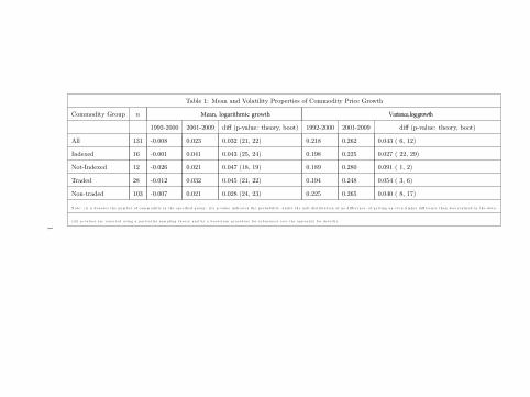
Table 1: Mean and Volatility Properties of Commodity Price Growth
Commodity Group n Mean, logarithmic growth Variance, log growth
1992-2000 2001-2009 di§ (p-value: theory, boot) 1992-2000 2001-2009 di§ (p-value: theory, boot)
All 131 -0.008 0.023 0.032 (21, 22) 0.218 0.262 0.043 ( 6, 12)
Indexed 16 -0.001 0.041 0.043 (25, 24) 0.198 0.225 0.027 ( 22, 29)
Not-Indexed 12 -0.026 0.021 0.047 (18, 19) 0.189 0.280 0.091 ( 1, 2)
Traded 28 -0.012 0.032 0.045 (21, 22) 0.194 0.248 0.054 ( 3, 6)
Non-traded 103 -0.007 0.021 0.028 (24, 23) 0.225 0.265 0.040 ( 8, 17)
N o t e : ( i ) n d e n o t e s t h e n um b e r o f c om m o d i t i e in t h e s p e c ifi e d g r o u p . ( i i ) p - va lu e in d ic a t e s t h e p r o b a b i l i ty, u n d e r t h e n u l l d i s t r ib u t io n o f n o d i§ e r e n c e , o f g e t t in g a n e v e n h ig h e r d i§ e r e n c e t h a n w a s r e a l i z e d in t h e d a t a .
( i i i ) p - va lu e s a r e r e p o r t e d u s in g a p a r t i c u la r s am p l in g t h e o r y a n d by a b o o t s t r a p p r o c e d u r e f o r r o b u s t n e s s ( s e e t h e a p p e n d ix fo r d e t a i l s ) .
1

Results from Previous Table• Consistent with aggregate data, the mean growth rates andvolatility of our price indeces higher in second sample.
— But, for most part are not statistically significant.— Exception: traded commodities that are not in a major index,show a significant jump in volatility.
• Not clear what to make of it.• Because they are traded goods, supports idea thatfinancialization changes price volatility.
• But, the fact that they are not included in index funds seemsto suggest that financialization stabilizes.
• Interestingly, traded goods are less volatile (though presumablynot significantly so) than non-traded goods, suggesting thatfinancialization stabilizes.
• We move on now, to the fully disaggregated data.

Structural Break Approach: Regressions
• For each commodity, regress log real spot price on time trendwith a break in 2000.
— Calculate the change in• the slope coeffi cient.• the standard deviation of the regression residual.
• Also calculate change in variance of commodity price growth.• Relate above to change in:
— open interest— net financial flows.

Change, Net Financial Flows0 1 2 3 4 5 6 7
Cha
nge,
spo
t pric
e tr
end
-0.3
-0.2
-0.1
0
0.1
0.2
0.3
0.4
0.5All commodities, slope = 0.022
Change, Net Financial Flows0 1 2 3 4 5 6 7
Cha
nge,
spo
t pric
e tr
end
0
0.05
0.1
0.15
0.2
Traded commodities, slope = 0.016
Change, Net Financial Flows0 0.1 0.2 0.3 0.4 0.5 0.6
Cha
nge,
spo
t pric
e tr
end
-0.3
-0.2
-0.1
0
0.1
0.2
Softs, slope = 0.144
Figure 4b: Change in Trend and Net Financial Flows
Change, Net Financial Flows0 1 2 3 4 5 6 7
Cha
nge,
spo
t pric
e tr
end
-0.1
0
0.1
0.2
0.3
0.4
0.5
Minerals and fuel, slope = 0.013

Calculation of P-value
• Bootstrap procedure.• P−value: probability, under null hypothesis that the scatterslope is zero, of getting a slope that is steeper than is observedin the data.

Table 2: Change in Commodity Inflation Dynamics, 1990s to 2000s, as a Function of Change in FinancializationP-value on when financialization measured with nff (P −value with oi)
change in commodity inflation dynamicst change in financializationut
variables in analysis change in variance of residual from time trend change in slope coefficient on time trend change in varianceall commodities 64 (66) 11 (15) 39 (48)indexed 76 (89) 14 (50) 39 (47)non-indexed 20 (18) 62 (14) 17 (18)traded 72 (78) 12 (21) 44 (56)softs 12 (32) 2 ( 4) 2 ( 9)minerals and fuels 76 (68) 24 (32) 67 (68)Notes: (i) two measures of financialization - net financial flows (nff) and open interest (oi). (ii) p-value is the probability, under the null distribution that 0, of getting a value of higher than its empirical realized value. For details, see the appendix.

Structural Break Approach
• Finding : (except for softs: corn, lumber, etc.) there is nosignificant relationship between a structual break in pricedynamics and change in financialization.

Centered Moving Average Approach
• Potential pitfall for structural break approach: it may besensitive to the (somewhat arbitrary) choice of 2000 as thebreak date.
• Our second (‘Centered Moving Average’) approach.— Compute a rolling standard deviation of the growth rate ofcommodity prices (5-point moving average).
— A shortcoming of this approach is you lose some data.

Centered Moving Average approach
• Regress volatility time series on financialization measures.
• Done only for commodities for which there is non-zero volumeof trade in each time period.

−4 −3 −2 −1 0 10
0.2
0.4
0.6
0.8
1
1.2
Figure 8: Response of Volatility to Two Measures of Volume(results based on individual traded commodities)
mean response of volatility to Net Financial Flows = −0.24
mean response of volatility to Open Interest = −0.06
Net Financial FlowsOpen Interest

Centered Moving Average approach
• Message of previous slide• distribution of response of volatility to financialization isdispersed.
• centered on negative numbers: more financialization results inless volatility.
— mean standard deviation over all variables is 0.2.— mean slope on open interest is -0.06.— raise open interest from one times world production to two,then volatility falls small amount, from 0.2 to 0.14.

Centered Moving Average approach
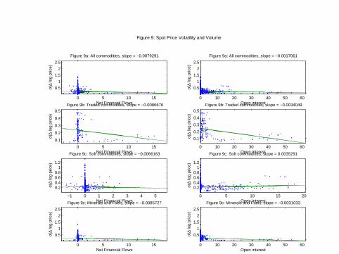
• The following figure displays scatter plot of all data in eachcategory: all, softs, minerals&fuels.
— Here, we included non-traded commodities.
• For example, in the ‘all’category, we have 13× 131observations.
0 5 10 15
0.5
1
1.5
2
2.5
Net Financial Flows
σ(∆
log
pric
e)
Figure 9a: All commodities, slope = −0.0079291
0 10 20 30 40 50 60
0.5
1
1.5
2
2.5
Open interest
σ(∆
log
pric
e)
Figure 9a: All commodities, slope = −0.0017061
0 5 10 15
0.1
0.2
0.3
0.4
0.5
Net Financial Flows
σ(∆
log
pric
e)
Figure 9b: Traded commodities, slope = −0.0086676
0 10 20 30 40 50 60
0.1
0.2
0.3
0.4
0.5
Open interest
σ(∆
log
pric
e)
Figure 9b: Traded commodities, slope = −0.0034049
−1 0 1 2 3 4 5
0.20.40.60.8
11.2
Net Financial Flows
σ(∆
log
pric
e)
Figure 9c: Soft commodities, slope = −0.0066163
0 5 10 15 20
0.20.40.60.8
11.2
Open interest
σ(∆
log
pric
e)
Figure 9c: Soft commodities, slope = 0.0035291
0 5 10 15
0.5
1
1.5
2
2.5
Net Financial Flows
σ(∆
log
pric
e)
Figure 9c: Minerals and Fuels, slope = −0.0085727
Figure 9: Spot Price Volatility and Volume
0 10 20 30 40 50 60
0.5
1
1.5
2
2.5
Open interest
σ(∆
log
pric
e)
Figure 9c: Minerals and Fuels, slope = −0.0031033

Centered Moving Average approach
• Message of previous slide
• No evidence that increased financialization raises volatility.— Indeed, the evidence suggests volatility may drop.— But, these effects are quantitatively small here.

Table 3: Regression, Volatility of Commodity Prices on Intensity of Financializationvolatilityt intensityt
intensity measurenet financial flows open interest
group of variables (95% conf interval) (95% conf interval)all commodities -0.001 (-0.024,0.029) 0.004 (-0.004,0.007)traded 0.009 (-0.019,0.033) 0.009 (-0.002,0.011)softs -0.007 (-0.028,0.027) 0.004 (-0.003,0.008)minerals and fuels 0.020 (-0.060,0.108) 0.005 (-0.014,0.028)Notes: (i) standard deviation based on centered, 7 point moving average of commodity price growth; (ii) data combines all observations on the group of
commodities listed in left column; (iii) we dropped silver and gold from the analysis underlying this table. See the text for discussion. (iv) bootstrap confidence intervals described in text.

Table 4: Another Way to See that Financialization Has Little Impact on Spot Price Volatility(1) (2)
Measure of financialization Measure of spot price dynamics12 month average oi growth centered, 6 month moving average standard deviation
2nd quartile interquartile range associated with column (1) quartileslower bound -1.499 4.471mean (median) -0.369 (-0.343) 7.426 (6.400)upper bound 0.690 9.062
3rd quartilelower bound 0.692 4.818mean (median) 1.875 (1.831) 7.857 (6.876)upper bound 3.178 9.573
14

Correlations Between Return on Futuresand 3 Month Tbills/Equity
• Study impact of financialization on volatility of commodityfutures returns and their comovement with other asset returns.
• Computed correlations of futures returns and other returns foreach year.
• Regress time series of correlations on financialization measuresfor each commodity.
• Finding: mean coeffi cients nearly zero.
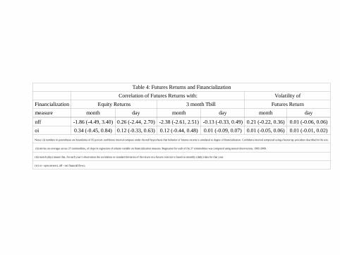
Table 4: Futures Returns and FinancializationCorrelation of Futures Returns with: Volatility of
Financialization Equity Returns 3 month Tbill Futures Returnmeasure month day month day month day
nff -1.86 (-4.49, 3.40) 0.26 (-2.44, 2.70) -2.38 (-2.61, 2.51) -0.13 (-0.33, 0.49) 0.21 (-0.22, 0.36) 0.01 (-0.06, 0.06)oi 0.34 (-0.45, 0.84) 0.12 (-0.33, 0.63) 0.12 (-0.44, 0.48) 0.01 (-0.09, 0.07) 0.01 (-0.05, 0.06) 0.01 (-0.01, 0.02)Notes: (i) numbers in parentheses are boundaries of 95 percent confidence interval compute under the null hypothesis that behavior of futures returns is unrelated to degree of financialization. Confidence interval computed using a bootstrap procedure described in the text.
(ii) entries are averages across 27 commodities, of slope in regression of column variable on financialization measure. Regression for each of the 27 commodities was computed using annual observations, 1992-2009.
(iii) month (day) means that, for each year’s observation the correlation or standard deviation of the return on a futures contract is based on monthly (daily) data for that year.
(iv) oi - open interest, nff - net financial flows;

Summary So Far
• There has been increased financialization in commoditymarkets.
• Cross sectional analysis shows little evidence thatfinancialization has had an effect on price behavior.
— This inference is subject to the usual caveats about drawinginferences about causality from cross-sections.
• Still need a detailed reconciliation of our findings with thosewho conclude that financialization has a substantial effect.

Relation to Tang and Xiong
• Tang-Xiong computed pairwise correlations between returns oncommodity futures.
— We compute pairwise correlations by centered moving average,j = −lag, ..., lag,
— lag = 130 days in daily correlations, lag = 6 months inmonthly data.
• Tang-Xiong found that the pairwise correlations were greaterfor indexed commodities and for non-indexed commodities.
— Concluded that financialization matters.
• We obtain similar findings for daily data, but differencesbetween indexed and non-indexed commodities appear to goaway in monthly data.

Next Slide, Pairwise Correlations in DailyReturns

1992 1994 1996 1998 2000 2002 2004 2006 2008 20100
0.05
0.1
0.15
0.2
0.25
0.3
0.35
0.4average return correlation among commodities
all commoditiesindexed commoditiesoff-indexed commodities
Next Slide, Pairwise Correlations inMonthly Returns

1992 1994 1996 1998 2000 2002 2004 2006 2008 2010-0.1
0
0.1
0.2
0.3
0.4
0.5
0.6average return correlation among commodities
all commoditiesindexed commoditiesoff-indexed commodities

Financialization and Futures Markets
• So far, we’ve found no systematic relationship betweenfinancialization and spot prices.
• Hong and Yogo (JFE, 2012) show a link betweenfinancialization and futures prices.
— Open interest helps to predict futures returns.— Net financial flows do not help to predict futures returns.
• We have a different way to demonstrate these links.

Measuring the Importance ofFinancialization in Futures Markets
• Fictitious investor adopts following strategy:— in month t, examine the volume of trade in commodity futuresup to month t− 1.
— go long in a basket of commodities that show the most volumeof trade (hot strategy).
— two measures of ‘volume of trade’:• ‘net financial flows’- net commercial trader shorts, divided byopen interest.
• growth of open interest over the past year.
• Compare hot net financial flow strategy ; hot open interestgrowth strategy; random strategy, random basket.

1970 1975 1980 1985 1990 1995 2000 2005
50
100
150
200
250
Cumulative returns from 3 futures contract strategiesNOTE : Shaded areas represent 90 percent confidence interval
Mode, random futures market strategy Hot net financial flow strategyHot open interest growth strategy

Finding:
• Open interest growth contains substantial information aboutsubsequent commodity returns.

Summary of Empirical Evidence
• There is substantial variation in the degree of financialization inthe cross section of commodities.
— there does not seem to be a systematic relationship betweenthe degree of financialization and spot price volatility.
• But, futures markets do seem to matter for futures returns.— The volume of open interest growth appears to reliably predicthigh subsequent futures returns.
— Net financial flows unrelated to subsequent futures returns.
• How could open interest affect futures returns without having asystematic effect on spot prices?

One Period Model• Futures markets allow agents to reduce risk by hedging.
— Insiders:• Farmers worry wheat prices, P, will be low.• Bakers worry that P will be high.
— Outsiders: care about P because correlated with their ownincome.
— Futures market: opens when wheat planted, with price F.Futures return - P− F.
• All market participants also ‘speculate’— Maximize mean-variance utility subject to constraints.— Solution: demand for long (short, if negative) contracts
= hedging demand +
speculative demand︷ ︸︸ ︷E (P− F)
αvar (P− F)
α ∼ risk aversion, same for everyone

Bakersbuywheat,bakebread
FarmersPlantseeds,growwheat
OutsidersNodirectpar<cipa<oninproduc<onoruseofcommodity
CommodityMarket

Bakers
Farmers
Outsiders
CommodityMarketSourceofuncertaintyforinsiders:Demandforbread–Θ+ε
Knownatbeginning
Realizedattheend

Bakers
Farmers
Outsiders
CommodityMarketSourceofuncertaintyforinsiders:Demandforbread–Θ+ε
Knownatbeginning
Realizedattheend
Sourceofuncertaintyforoutsiders:outsideincome,x,correlatedwithε.

Bakers
Farmers
Outsiders
Hedgingmo<ve:Uncertaintyinpriceofwheat,P.Wanttobuylonginfuturesmarket.Hedgingneedlimitedbecausebreadpriceisanaturalhedge.
CommodityMarket

Bakers
Farmers
Outsiders
Hedgingmo<ve:UncertaintyinP.Wanttosellshortinfuturesmarket.
Hedgingmo<ve:Uncertaintyinpriceofwheat,P.Wanttobuylonginfuturesmarket.Hedgingneedlimitedbecausebreadpriceisanaturalhedge.
CommodityMarket

Bakers
Farmers
Outsiders
Hedgingmo<ve:UncertaintyinP.Wanttosellshortinfuturesmarket.
Hedgingmo<ve:Uncertaintyinpriceofwheat,P.Wanttobuylonginfuturesmarket.Hedgingneedlimitedbecausebreadpriceisanaturalhedge.
Hedgingmo<ve:Cov(income,P)<0,golong.Cov(income,P)>0,goshort.Covariancechangesover<me.
CommodityMarket

Bakersbuywheat,bakebread
FarmersPlantseeds,growwheat
OutsidersNodirectpar<cipa<oninproduc<onoruseofcommodity
CommodityMarket
NetfinancialFlows,nff:Netpurchasesoflongcontractsbyoutsiders.
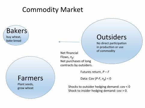
Bakersbuywheat,bakebread
FarmersPlantseeds,growwheat
OutsidersNodirectpar<cipa<oninproduc<onoruseofcommodity
CommodityMarket
NetfinancialFlows,nff:Netpurchasesoflongcontractsbyoutsiders.
Shockstooutsiderhedgingdemand:cov<0Shocktoinsiderhedgingdemand:cov>0.
Futuresreturn,P–F
Data:Cov(P-F,nff)=0

Lack of Pattern Across Markets BetweenFinancialization and Spot Price Volatility• There is a panel of markets in the cross section.
— Each market has a different mix of insider and outsider hedgingdemand shocks.
• Exogenous variations in measure of outsiders.— If most hedging demand shocks are to insiders, then outsidersstabilize price volatility.
— Otherwise, outsiders destabilize.• Endogenize outsider participation decision.
— Relation between participation and spot price volatilityambiguous.
— Example: small increase in shock volatility from a point wheremost shocks are to hedging demand by insiders.• direct effect (e.g., holding measure of outsiders constant): raiseprice volatility.
• entry effect: by increasing outsider participation, stabilize pricevolatility.

Conclusion
• Little evidence of a systematic relation, across commoditymarkets, between financialization and volatility.
— Some modest evidence that volatility is lower withfinancialization.
• We described a (fairly standard) model to interpret theobservations
— According to the theory, there is no reason to presume thatfinancialization will increase or decrease volatility of spot prices.
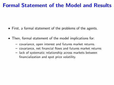
Formal Statement of the Model and Results
• First, a formal statement of the problems of the agents.
• Then, formal statement of the model implications for:— covariance, open interest and futures market returns.— covariance, net financial flows and futures market returns— lack of systematic relationship across markets betweenfinancialization and spot price volatility.
Agents in the Model
• Measure one of farmers produce wheat.
• Measure one of bakers produce bread from wheat.
• Measure µ of outsiders participate in futures markets for wheat.

Timing in the Model
• Beginning of Period:— Anticipated component of demand for bread, θ, realized.— Anticipated component of outsiders’income, s, realized.— then:
• Farmers choose how much wheat to produce.• Futures market meets.
• End of period:— Unanticipated shocks, η and ν, realized.— Unanticipated component of demand: ε ≡ η + ν.— Unanticipated component of outsiders’income: η.
• All shocks independent of each other.

Demand and Technology• Demand for bread
PQ = D (Q, θ + ε) ,
where PQ ∼ price of bread, Q ∼ quantity of bread.• Technology for producing bread from wheat, q :
Q = qδ, 0 < δ < 1.
• Cost function for producing wheat:
c (q) = cq+12
cq2, c, c > 0.
• All agents have mean-variance preferences over consumption, z :
Ez− α
2var [z]

Farmer’s Problem• Conditional on θ and s, farmers choose q and Hw to solve
max E [Pq+ RHw]− α
2var [Pq+ RHw]− c (q) ,
— Hw ∼ quantity of wheat futures bought.— P ∼ spot price of wheat.— R ∼ return on long futures contract,
R = P− F.
• Solution:
F = c′ (q)
Hw =
hedging demand︷︸︸︷−q +
speculative demand︷ ︸︸ ︷ER
αvar (R).

Baker’s Problem• End of period problem:
maxq
PQqδ − Pq.
— first order condition:
δPQqδ−1 = P.
— profits at optimum: (1δ− 1)
Pq.
• Beginning of period problem:
maxHb
E[
Pq(
1δ− 1)+ RHb
]− α
2var[
Pq(
1δ− 1)+ RHb
].
— solution:
Hb =
hedging demand︷ ︸︸ ︷q(
1− 1δ
)+
speculative demand︷ ︸︸ ︷ER
αvar (R).

Outsider’s Problem• Outsiders’income, x, given by
x = −sη.
— outsiders’income is partially correlated with unanticipatedcomponent of demand for bread, ε = η + v.
— correlation varies with realization of s.— leads to fluctuation in outsiders’hedging demand.
• Outsiders’futures market problem, conditional on θ and s :
maxHo
E [RHo − sη]− α
2var [RHo − sη] .
— solution:
Ho =
hedging demand︷︸︸︷s
σ2η
σ2ε
+
speculative demand︷ ︸︸ ︷ER
αvar (R).
• Note: if σ2η = 0, then outsiders have no hedging demand.

Futures Market Price Determination
• Market clearing condition:
Hw +Hb + µHo = 0.
• Induced demand function for wheat using bakers’fonc:—
P = D(
qδ, θ + ε)
δqδ−1.
• We work with linearized representation:
P = D0 −Dqq+ θ + ε.
• Yields linear equilibrium solutions for equilibrium prices andquantities.

Equilibrium Solutions• Futures return (R = P− F) :
R = R0 + Rθθ + Rss+ ε,
• Production decision:
q = q0 + qθθ + qss.
• Lemma:Rθ > 0, Rs < 0 and qθ, qs > 0.
• Open interest, oi, given by:
oi =12
[|Hw|+
∣∣∣Hb∣∣∣+ µ |Ho|
].
• Net financial flows, nff , given by:
nff = µHo.

Open Interest and Net Financial Flows
• Proposition: there exists σ2s such that cov (nff , R) = 0.
— Basic idea of proof:• s shocks drive R(= P− F) down and nff up• θ shocks drive R up and nff up.
• Proposition: Suppose Hb, Ho > 0 for all realizations of shocksand µ not too large, then cov (oi, R) > cov (nff , R)— Basic idea of proof:
• When θ goes up, farmers go short and, since µ small, bakersmust go long, Hb up, R up.
• When s goes up, outsiders go long (so, R down), insiders goshort (Hb down).

Var(P) and Exogenous Participation• Variance of spot prices, var (P) , given by: δc+ ασ2
ε2+µ
δ(c+Dq
)+ ασ2
ε2+µ
2
σ2θ+
δDq
(1− 2
2+µ
)ασ2
η
δ(c+Dq
)+ ασ2
ε2+µ
2
σ2s +σ2
ε .
• Proposition: If σ2θ small, outsiders destabilize spot prices.
— recall, F = c′ (q) .— F and so q respond more to s, so P more variable.
• Proposition: If σ2η or σ2
s small, outsiders stabilize spot prices.— F and so q respond more to θ, so P more stable.
• Increase in outsiders may stabilize or destabilize.— Depends on market details.

Endogenizing Outsider Participation
• Outsiders have fixed cost, k, of entering each futures market.
• Enter before any shocks realized.
• Enter if surplus, S = UP −Unp, from participation exceedscost:
S ≥ k.
• Let k∗ denote fixed cost of marginal entrant.
Equilibrium condition:F (S) = µ.
Endogenizing Outsider Participation
• Holding µ fixed, S is increasing in σ2θ and σ2
s .
• If s large and µ small, S is decreasing in σ2ε .
• Decompose overall effect on var (P) into direct effect and entryeffect.
— Direct effect: holds µ fixed, varies parameter.— Entry effect: holds parameter fixed, varies µ.— Overall effect ambiguous if direct and entry effect haveopposite sign.

Endogenizing Outsider Participation
• Proposition: if σ2η small, increase in σ2
θ or σ2s has ambiguous
effect on var (P) .
• Proposition: if σ2θ small, s large and µ small, increase in σ2
ε hasambiguous effect var (P) .
• Our model consistent with absence of systematic relationshipacross markets between nff and var (P).


