Financial Innovations and EndogenousGrowth

Yuan K. Chou and Mart in S. ChinUniversity of Melbourne

July 30, 2001

Abstract

This paper explores the channels through which innovations in thefinancial sector lead to economic growth. The channels identified arecapital accumulation and technological innovation. The first is fulfilledby financial intermediaries which transform household savings into pro-ductive investment by firms, the second by venture capitalists whichfund risky technological projects with high potential payoffs. The rateof financial innovation is determined by the amount of labor (or humancapital) devoted to the sector as well as by spillovers from existing fi-nancial products. By embedding such a sector into the Romer (1990) -Jones (1995) and Lucas (1988) - Uzawa (1965) frameworks, it is shownthat ultimately, financial innovations can only lead to long-run growththrough its venture capital role. The transformative role of the finan-cial sector only leads to temporary growth effects on the transitionalpath to the steady state.

Keywords: Economic Growth, Finance, Technological ChangeJEL Codes: G20, O31, O33, O41

1 Introduction

Why does the financial sector matter to the real economy? The ever-risingnumber of graduates from top American and European universities beingrecruited by financial powerhouses and their handsome remuneration lendcredence to the suggestion that the financial sector must be a highly valu-able engine of growth in an advanced economy. Extensive media coverageof the activities of the finance industry seem to confirm its pre-eminence.Even in the other pillar of the New Economy, the real technological sec-tor, financial firms in the guise of venture capitalists are seen as the keyto inducing high-risk, potentially high-return ideas and innovations. How-ever, the standard theoretical growth literature (including the New GrowthTheory of the last fifteen years) notably excludes any meaningful role forthe financial sector to influence long-run growth. Savings by householdsare automatically assumed to be transformed into productive investment

1

by firms at every point in time by appealing to the “savings equal invest-ment in equilibrium” argument. The vast majority of papers that have beenwritten on the “finance-growth nexus” describe microeconomic models thatdetail how financial institutions alleviate borrowing constraints, perform riskmanagement, acquire information to assist in resource allocation, monitormanagers, mobilize savings and lead to rising specialization and efficiency inproduction. There is also an extensive literature on the empirical evidencelinking development of the finance sector to economic growth [see, for exam-ple, Arestis and Demetriades (1997), Demetriades and Hussein (1996) andKing and Levine (1993a)].

This paper aims to fill that important gap in the literature by explain-ing how a financial sector can be incorporated into an endogenous growthmacroeconomic model such as those by Romer (1990) and Lucas (1988).Just as Romer constructs a dynamic equation describing the productionof new designs or blueprints in the research and development sector, wedevelop a dynamic equation describing the production of financial innova-tions that continuously improves the efficiency of the intermediation processwhich transforms savings into investment and lubricates R&D activities inthe real technological sector. In addition, the financial innovations sectormay also be modelled in competition with a human capital producing sectorfor that scarce resource a là Lucas. We also explain the complicated ways inwhich households, financial innovators, financial intermediaries, R&D firms,intermediate and final goods producers interact and are intertwined in ourmodel of the macroeconomy. Finally, we distinguish between the competi-tive, decentralized solution and that of a hypothetical social planner.

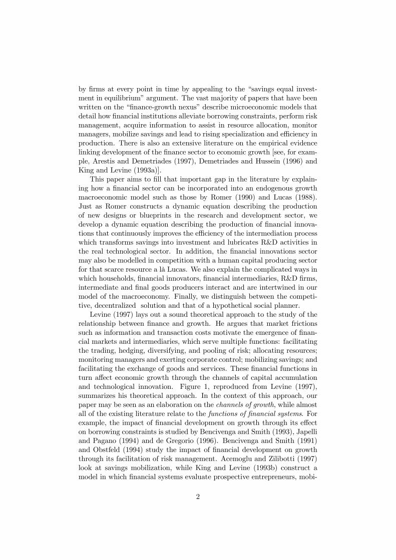
Levine (1997) lays out a sound theoretical approach to the study of therelationship between finance and growth. He argues that market frictionssuch as information and transaction costs motivate the emergence of finan-cial markets and intermediaries, which serve multiple functions: facilitatingthe trading, hedging, diversifying, and pooling of risk; allocating resources;monitoring managers and exerting corporate control; mobilizing savings; andfacilitating the exchange of goods and services. These financial functions inturn affect economic growth through the channels of capital accumulationand technological innovation. Figure 1, reproduced from Levine (1997),summarizes his theoretical approach. In the context of this approach, ourpaper may be seen as an elaboration on the channels of growth, while almostall of the existing literature relate to the functions of financial systems. Forexample, the impact of financial development on growth through its effecton borrowing constraints is studied by Bencivenga and Smith (1993), Japelliand Pagano (1994) and de Gregorio (1996). Bencivenga and Smith (1991)and Obstfeld (1994) study the impact of financial development on growththrough its facilitation of risk management. Acemoglu and Zilibotti (1997)look at savings mobilization, while King and Levine (1993b) construct amodel in which financial systems evaluate prospective entrepreneurs, mobi-

2

lize savings to finance the most promising productivity-enhancing activities,and diversify the risks associated with these innovative activities, therebyimproving the probability of successful innovation. Similarly, Saint-Paul(1992) looks at how capital markets facilitate the adoption of more special-ized and productive technologies. Broadly speaking, our paper complementsthe existing literature by telling a macroeconomic story of how the produc-tion of financial innovations affect growth through capital accumulation andtechnological innovation, while the existing literature provide rich detailedexamples of how financial markets and intermediaries fulfil their financialfunctions from a microeconomic perspective.

Figure 1: Levine’s (1997) Theoretical Approach to Finance and Growth

The paper is organized as follows: the next section describes a basicgrowth model with a financial sector and derives its analytical solution.Section 3 delves into the details of a growth model with both endogenoustechnological progress and financial innovations, explaining the decentral-ized model in considerable detail, and explores the comparative statics of itssolution. Section 4 examines a model with human capital and financial inno-vations and graphs the implications of its solutions, while Section 5 discussesthe policy implications arising from these models. Section 6 concludes.

3

2 The Basic Model

To isolate the workings of our proposed financial sector, we first embed it in astandard no-frills growth model with intertemporal household optimizationbut without endogenous technological progress. We will see that, unsur-prisingly, the model is incapable of generating endogenous growth in thesteady-state. The efficiency and development of the financial sector gener-ates non-zero growth in per-capita variables only on the transitional path tothe steady state. Moreover, changes in the production function of financialinnovations (or new financial products) generate only level but not growtheffects.

The financial sector in this model comprises financial innovators andfinancial intermediaries. The former produce new financial “blueprints”(products and services) using labor that is diverted from the production ofthe final consumption good. These “blueprints” include innovations such asATMs, phone and internet banking, derivatives of existing financial prod-ucts (including new options), initial public offerings (IPOs) of companiesand anything which enables funds to be channelled more effectively fromsavers (households) to borrowers (firms seeking to raise capital to financethe purchase of new plant and equipment). We denote the stock of financialproducts (ie. old financial innovations) as τ . Analogous to the Romer (1990)specification of the real R&D sector, the development of the financial sectoris characterized by an ever-expanding variety of financial products. For sim-plicity, there is no “creative destruction” of existing financial products bysuccessively superior products That is, there are no quality ladders in finan-cial products. However, the existing stock of financial innovations/productsaffect the production of new financial ideas according to

τ = F (uτL)λτφ,

where uτ is the fraction of the labor force employed by the financial sector,and F, λ,and φ are constants.

The idea is that of a spillover effect from each financial innovation: fi-nancial innovators may build upon the ideas of other innovators to create adifferentiated or improved financial product.

Financial intermediaries, on the other hand, are responsible for inter-mediating funds between borrowers and lenders. Borrowers are produc-ers of the final consumption good while lenders are households with sav-ings. The efficiency at which savings can be transformed into productiveinvestment is specified to be dependent on the existing stock of financialinnovations/products per adjusted capita (τ/Lκ, which we will label as ξ,0 < κ < 1), which proxies for the state of development and sophistication of

4

the financial sector. The capital accumulation function hence looks like:

K (t) =τ (t)

L (t)κ

hAK (t)α (uY (t)L (t))

1−α −C (t)i− δK (t) ,

whereK is the stock of capital, L is the number of workers, A is a (constant)technological parameter, and uY is the share of labor devoted to final goodsproduction.1 By including κ in our measure of transformative efficiency ξ, weare acknowledging that some financial innovations may be rivalrous (such asthe creation of each new IPO, which may benefit from the knowledge gainedfrom previous IPOs but nevertheless requires new labor to be expended inorder to tailor it to the needs of individual firms) while others are not (suchas a new financial instrument, which may in fact benefit from “thick market”effects as it becomes more widely traded). By restricting κ to lie strictlybetween 0 and 1, we are saying that in the aggregate, financial innovationsor products are neither fully rivalrous nor fully non-rivalrous.2

In the steady state, τ/Lκ must be constant by definition. Therefore,if the labor force grows at the constant rate n, then the rate of financialinnovations in the steady state must equal κn. Why must the number offinancial products continually increase in the steady state even when allsavings are completely transformed into investment? We argue that as thelabor force or population increases, so does the volume of funds that haveto be intermediated. Due to the rivalrous nature of some financial productsand services, this rising volume results in congestion and decreased efficiencyin the financial sector unless more financial products are devised to alleviatethe strain on it. Loosely speaking, resources such as labor must continue tobe directed to the financial sector as it services an expanding economy.

2.1 The Social Planner’s Problem

We now proceed to lay out the social planner’s problem and discuss thesteady-state solutions of the model. The social planner seeks to maximizethe representative consumer’s stream of discounted utility assuming a Con-stant Relative Risk Aversion (CRRA) utility function:

maxc(t),uY (t)

U0 =

Z ∞

0

c (t)1−θ − 11− θ e−ρtdt, (1)

1Pagano (1993) speciøes the saving-investment relat ionship as φS = I, where 1− φ isthe Æow of saving �lost�in the process of ønancial intermediat ion. This (exogenous, in hiscase) fract ion goes to banks as the �spread between lending and borrowing rates, and tosecurit ies brokers and dealers as commissions, fees and the like�(pp. 614-615).

2I f κ = 1, then all ønancial products are st rict ly rivalrous; if κ = 0, then all ønancialproducts are st rict ly non-rivalrous, so that the e�ciency of ønancial intermediat ion isdependent only on the stock of ønancial products and independent of populat ion size.

5

where c ≡ C/L, subject to

K (t) =τ (t)

L (t)κ

hAK (t)α (uY (t)L (t))

1−α −C (t)i− δK (t) , (2)

τ (t) = F [(1− uY (t))L (t)]λ τ (t)φ , (3)

where

L (t) = L (0) ent. (4)

Note that α ∈ (0, 1), uY (t) ∈ [0, 1] ∀t and {θ, ρ, δ, n} > 0.

2.1.1 Model Set-Up

The Hamiltonian is

H ≡ c1−θ − 11− θ e−ρt + ν

h τLκ¡AKαu1−αY L1−α −C¢− δKi

+µF (1− uY )λLλτφ, (5)

where the control variables are c and uy, the state variables are K and τ ,and ν and µ are the costate variables associated with K and τ respectively.The first-order conditions for the control variables are

∂H

∂C= c−θe−ρt − ντ = 0, (6)

∂H

∂uy= ντAKα (1− α)u−αY L1−α−κ − µFλ (1− uY )λ−1Lλτφ = 0. (7)

The first-order conditions for the state variables are

K

K=

τ

Lκ

µAKα−1u1−αY L1−α − C

K

¶− δ, (8)

τ

τ= F (1− uY )λLλτφ−1. (9)

The first-order conditions for the costate variables are

ν = −∂H

∂K= −ν ¡τAαKα−1u1−αY L1−α−κ − δ¢ , (10)

µ = −∂H

∂τ= −ν

µAKαu1−αY L1−α−κ − C

Lκ

¶(11)

−µF (1− uY )λLλφτφ−1. (12)

Finally, the transversality conditions are

limt→∞ν (t)K (t) = 0, (13)

limt→∞µ (t) τ (t) = 0. (14)

6

2.1.2 Variables in the Steady State

To arrive at the steady-state solutions, we first define the following threevariables k ≡ K/L, χ ≡ C/K and ξ ≡ τ/Lκ. In the steady state, werequire the output-capital ratio given by

Y

K= Akα−1u1−αY , (15)

to remain constant. This implies, from equation (15), that

Y

Y− KK= (α− 1) k

k+ (1− α) uY

uY= 0. (16)

We also require that uY /uY = 0 in the steady state. Hence, k/k = 0 as wellin order to satisfy equation (16), so the growth rate of output per capitay/y is zero. Furthermore, it is assumed that χ/χ = ξ/ξ = 0 in the steadystate. Since L grows at the exogenous rate n according to equation (4),these assumptions imply that, to have a balanced growth path, we musthave Y /Y = K/K = C/C = n and τ/τ = κn in the steady state. Fromτ = FuλτL

λτφ, we have γτ ≡ τ/τ = FuλτLλτφ−1. Taking logarithms of thelatter equation and differentiating both sides with respect to time provideus the solution to the steady-state growth rate of τ , γ∗τ = λn/ (1− φ).Since τ/τ = κn, the solution implies that κ = λ/ (1− φ). The steady-state growth rate of n is comparable to the Cass (1965) - Koopmans (1965)formulation of the Solow (1956) - Swan (1956) model without technologicalprogress. In their model, the absence of technological progress eventuallyresults in aggregate output growing at rate n since there are no increases inproductivity to offset the diminishing marginal product of physical capital.Here, output grows at rate n in the steady state since there are limits to theefficiency of financial innovations in transforming the flow of savings to newphysical capital.

The model is solved in terms of the four unknowns k, χ, ξ and uY . Thefour equations needed to pin down the solutions to the four unknowns aregiven by k/k = 0, χ/χ = 0, ξ/ξ = 0 and uY /uY = 0. These four conditionslead to the following equations respectively:

ξAkα−1u1−αY − ξχ = n+ δ, (17)

ξAαkα−1u1−αY = ρ+ n+ δ, (18)

F (1− uY )λ ξφ−1 =λn

1− φ , (19)

λ2n

(1− α)(1− φ)uY

1− uY£1− ¡ξ−1A−1k1−αuα−1Y

¢ξχ¤

= ξAαkα−1u1−αY − δ − (1− λ)n. (20)

7

2.1.3 Analytical Solutions to the Model

Using equations (17) to (20), we obtain the following solutions for uY , uτ ,ξ, χ and k:

u∗τ =Γ

Γ+Φ, (21)

where Γ ≡ αλγ∗τ (n+ δ), Φ ≡ (1−α) (ρ+ λn) (ρ+ n+ δ), γ∗τ = λn/ (1− φ),

u∗Y = 1− u∗τ=

Φ

Γ+Φ, (22)

ξ∗ =

·Fu∗λτγ∗τ

¸ 11−φ

(23)

=

"F

γ∗τ

µΓ

Γ+Φ

¶λ# 11−φ

, (24)

χ∗ =ρ+ (1− α) (n+ δ)

αξ∗

=ρ+ (1− α) (n+ δ)

α

"γ∗τF

µΓ+Φ

Γ

¶λ# 11−φ

, (25)

k∗ =

µξ∗Aα

ρ+ n+ δ

¶ 11−α

u∗Y

=

Aα

ρ+ n+ δ

"F

γ∗τ

µΓ

Γ+Φ

¶λ# 11−φ

11−α

Φ

Γ+Φ. (26)

2.2 Implications of the Model

Proposition 1 The financial innovations sector has no influence on thesteady-state growth rate of the economy.

In the steady state, the variables Y , K, and C all grow at the rate n,the population growth rate, in order to achieve a balanced growth path,while τ grows at rate κn. In spite of its role in transforming funds intoproductive investments, the financial innovations sector does not alter thebalanced growth path requirement at all.

We relegate the proofs of the following propositions to the Appendix.

8

Proposition 2 The steady-state proportion of labor employed in the finan-cial innovations sector, u∗τ , is lower in the decentralized economy than in thesocial planner’s case.

The divergence arises because the social planner internalizes the spillovereffects of existing financial products on financial innovations.

We now discuss the implications of the model with regard to the steady-state proportion of labor employed in the financial innovations sector, u∗τ .We specifically investigate the impact on u∗τ of a change in the followingparameters: (i) the spillover parameter in the financial innovations sector,φ; (ii) the rate of time preference, ρ; and (iii) the degree of risk aversion, θ.

Proposition 3 An increase in the financial innovations spillover effect, φ,increases the steady-state proportion of labor employed in the financial in-novations sector, u∗τ .

An increase in φ raises the marginal product of labor of financial innova-tors. The share of labor in the financial innovations sector must thus rise sothat the wage in this sector once again equals that of the final goods sectorin the new equilibrium.

Proposition 4 An increase in the rate of time preference (or households’discount factor), ρ, decreases the steady-state proportion of labor employedin the financial innovations sector, u∗τ .

As households become more impatient, they care more for current con-sumption then future consumption. Hence, more labor is devoted to thefinal goods sector to produce the final consumption good, and correspond-ingly less labor is devoted to the financial innovations sector..

Proposition 5 The degree of risk aversion, θ, does not affect the steady-state proportion of labor employed in the financial innovations sector, u∗τ .

2.3 Transitional Dynamics

To discuss the properties of the model away from the steady state, we needto reduce the dimensionality of the problem by assuming that the share oflabor in the financial innovations sector, uτ , and the physical investmentrate, sK , are constant and exogenous. The model then reduces to

Y = AKα(1− uτ )1−αL1−αK = ξsKY − δKτ = FuλτL

λτφ.

9

In the steady state, k = ξ = 0. The k = 0 and ξ = 0 schedules are given by

k∗ =

·ξ∗sKAn+ δ

¸ 11−α

(1− uτ )

ξ∗ =

·Fuλτ (1− φ)

λn

¸ 11−φ

and are plotted in the phase diagram below:

Figure 2: Transitional Dynamics of the Basic Model

Suppose the productivity parameter in the production function for finan-cial innovations, F, increases, possibly due to efficiency-promoting deregu-lation of the financial sector The rise in F shifts the ξ = 0 schedule to theright but leaves the k = 0 schedule unchanged. >From the diagram below,we see that both k and ξ must rise smoothly along the saddle path to theirnew levels. The increase in F has no effect on the long-run growth rates of kand y (which still remain at zero because there is no technological progress),but it has temporary growth effects in the transition to the new steady stateat higher levels of k∗ and y∗.

10

Figure 3: Transitional Dynamics for an Increase in F

3 Financial Innovations and Endogenous Techno-logical Progress

We now examine a full-blown growth model with a financial sector akin tothat in the previous section as well as endogenous technological progress inthe mold of Romer (1990) and Jones (1995). In this class of models, tech-nological progress is characterized by an increasing variety of intermediategoods used in the production of the final consumption good. Unlike the“creative destruction” models of Aghion and Howitt (1992) and Grossmanand Helpman (1991c), the producers of these intermediate goods never losethe monopoly rights to their production nor are they ever superseded by newproducers. The blueprints for new intermediate goods are in turn created bya real research and development sector which draws labor away from finalgoods production.

We allow for the stock of financial innovations, τ , to influence the rate atwhich new designs for intermediate goods are produced in the R&D sector.Implicitly, we are using the stock of financial innovations as a proxy for thestage of development of an economy’s financial sector: a more sophisticatedfinancial sector is associated with a higher innovation rate. This formulationattempts to capture the role that venture capitalists play in encouraginghigh-risk R&D activities with potentially large technological payoffs. Weargue that these venture capital firms are only ubiquitous in economies withhighly-developed and sophisticated financial sectors.

As before, the financial sector consists of financial innovators who createnew financial products, and financial intermediaries who use the existing

11

stock of financial products to intermediate funds between households andfirms by transforming the savings of the former into productive investmentby the latter. Unlike the model discussed in the previous section, however,now financial intermediaries (or more accurately, their venture capitalistarms) also extract rents from the real R&D sector for identifying and fi-nancing high-risk research projects with potentially huge future pay-offs.For tractability’s sake, we do not differentiate between financial innovationswhich improve the efficiency of the intermediation process and those whichmake the financing of ever-riskier projects possible.

In the rest of this section, we first present the decentralized, competitivemodel, followed by a discussion of the characteristics and implications ofthe planner’s solution. The decentralized model will explain how the dif-ferent actors (households, final goods firms, intermediate goods producers,real R&D firms, financial intermediaries and financial innovators) and con-stituent components of the model function and interact. A flowchart of themodel is illustrated in Figure 2.

3.1 The Decentralized Model

As in Jones (1995), the final goods sector produces the consumption goodY using labor uY L and a collection of intermediate inputs x, taking theavailable variety of intermediate inputs A as given:

Y = (uY L)1−α

Z A

0x (i)α di. (27)

This specification of the production function characterizes technologicalchange as increasing variety, as in Dixit and Stiglitz (1977). Inventions arebasically the discovery of new varieties of producer durables that providealternative methods of producing the final consumer good.

A representative producer of final goods solves the following profit max-imization problem

maxuY ,x(i)

πY = (uY L)1−α

Z A

0x (i)α di−wY uYL−

Z A

0p (x (i))x (i) di, (28)

where wY is the prevailing wage in the final goods sector and p (x (i)) is theprice of intermediate good i. The price of the final good is normalized tounity. The first-order conditions dictate that

wY = (1− α) Y

AuY L, (29)

and

p (x (i)) = αu1−αY L1−αx (i)α−1 ∀i. (30)

12

The intermediate sector comprises an infinite number of firms on theinterval [0, A] that have purchased a design from the real R&D sector, nowacting as monopolists in the production of their specific variety. FollowingRomer (1990) and Jones (1995), each firm rents capital at rate rK and,using the previously purchased design, effortlessly transforms each unit ofcapital into a single unit of the intermediate input. (For simplicity, producerdurables are transformed costlessly back into capital at the end of the periodand no depreciation takes place.) Each intermediate firm therefore solvesthe following problem period-by-period:

maxxπx = p (x)x− rKx. (31)

Being monopolists, they see the downward-sloping demand curve for theirproducer durables generated in the final goods sector. This results in a stan-dard monopoly problem with constant marginal cost and constant elasticityof demand, giving rise to the following solutions:

p (i) = p =rKα

∀i, (32)

x (i) = x =

"α (uY L)

1−α

p

# 11−α

∀i, (33)

and

πx(i) = πx = (1− α) px = α(1− α)Y

A∀i. (34)

Each intermediate firm thus sets the same price and sells the same quantityof its produced durable. Moreover, since

K =

Z A

0xdi = Ax, (35)

we can rewrite the aggregate final goods production function as

Y = Kα (AuY L)1−α . (36)

Next, we examine the production of new designs in the real R&D sector.Here, the rate of innovation is governed by the following production function

A = eB [(1− uY − uτ )L]η τβ , (37)eB ≡ BAψ, (38)

where (1− uY − uτ ) is the share of labor devoted to the production of newtechnical designs. In the decentralized model, R&D firms do not take intoaccount spillovers from existing designs, Aψ, so they regard eB as exoge-nously given. As argued previously, a more sophisticated financial sector

13

(with a greater stock of financial innovations, τ) is associated with a higherinnovation rate.

Each R&D firm derives revenue from the sale of blueprints to intermedi-ate goods producers, PAA, and incurs costs wA (1− uY − uτ )L from laborhired, and Rτ τ from services rendered by financial intermediaries. Its profitsare therefore

πA = PAA−wA (1− uY − uτ )L−Rττ , (39)

where L and τ are both compensated according to their marginal produc-tivities in R&D production:

wA = PABη [(1− uY − uτ )L]η−1 τβ, (40)

Rτ = PAB [(1− uY − uτ )L]η βτβ−1, (41)

where wA is the prevailing wage in the real R&D sector, Rτ is the “rentalrate” of τ charged by financial intermediaries, and PA is the price of eachnew technical design.

In our model, the financial sector is composed of financial innovators andfinancial intermediaries-cum-venture capitalists. The former are responsiblefor producing financial innovations, τ , which then determines the degree ofsophistication of the financial sector, proxied by ξ (equal to the ratio τ/Lκ,or the number of financial innovations per adjusted capita). A greater valueof ξ allows more efficient intermediation between lenders (households) andborrowers (intermediate goods producers), resulting in a higher percentageof savings being transformed into useful capital. In addition, a greater valueof ξ also raises the rate at which new R&D designs are produced, as explainedpreviously.

Financial innovators are monopolists who make extra-normal profits byproducing new financial products, using raw labor as input, according tothe production function

τ = eF (uτL)λ , (42)

where

eF ≡ Fτφ.As in the real R&D sector, financial innovators do not internalize the spillovereffect from the existing stock of financial products. They therefore treat eFas exogenously given.

The profit of a representative financial innovator, to be maximized byits choice of uτ , is

πτ = Pτ τ −wτuτL, (43)

14

where Pτ is the price of each financial innovation. Since ξ is constant in thesteady state (and specifically equals 1), τ/τ = κn in the steady state. Withthese substitutions, the first order condition dictates that

pτ ≡ PτAL1−κ

=wτuτξλγ∗τ

, (44)

where n is the population growth, wτ = wτ/A, ξ ≡ τ/Lκ and γ∗τ =λn/ (1− φ). From this equation, we see that the price of each financialinnovation is simply a constant mark up on the marginal factor cost of laborin the financial innovations sector.

Downstream in the financial sector, financial intermediaries purchase in-novations from financial innovators (which, in the real world, are probablysister divisions in the same financial firms) and use them in transformingsavings into productive investment as well as in the funding of real R&Dactivities. The financial intermediaries derive their income from: (a) charg-ing the R&D firms the rate Rτ to finance their production of new designs;and (b) by charging firms in the (real) intermediate sector a higher interestrate (rK) for renting capital than it pays out to households for their sav-ings (rV ). The interest rate differential, (rK − rV ), may be thought of asthe commission charged for intermediating funds. For simplicity, we assumethat financial intermediation requires no labor input. Financial intermedi-aries make zero profits as this sector is assumed to be perfectly competitive.

In each period, the representative financial intermediary ensures thatrevenues received from the real intermediate sector and R&D firms equalthe cost of acquiring deposits from households and purchasing new productsfrom financial innovators:

rKK +Rττ = rVK + Pτ τ . (45)

Finally, to close the model, we examine the consumption decision of house-holds. As usual, we assume that this decision may be characterized by arepresentative consumer maximizing an additively separable utility functionsubject to a dynamic budget constraint. We use a conventional CRRA util-ity function and assume that households are ultimate owners of all capitaland shareholders of final goods firms, real intermediate firms, R&D firms,financial intermediaries and financial innovators. The optimization problemis thus:

maxc,uY ,uτ

Z ∞

0

c1−θ − 11− θ e−ρtdt, (46)

subject to

V = rVK +wY uY L+wτuτL+wAuAL

+Aπx + πτ + πA − PAA−C, (47)

K = ξV , (48)

15

where V represents the flow of households’ stock of assets (i.e. saving), πx,πτ and πA are the monopolistic profits from the real intermediate sector,the financial innovators and the R&D sector respectively. The monopolis-tic pofits of financial innovators, πτ , equal to revenue Pτ τ , less labor costswτuτL, is paid out to households who are alsoshareholders of these firms.Unlike Jones (1995), the real R&D sector is also allowed to generate monop-olistic profits which again accrue ultimately to households. In equilibrium,wages are equal across all labor markets, i.e. wY = wτ = wA = w. Theseconditions together with equation (45) yield the following households budgetconstraint

K = ξ (rKK + wuY L+ wuAL+Rττ

+Aπx + πA − PAA−C´. (49)

We can show that the prices of R&D blueprints and financial innovationsare determined by the following arbitrage equations respectively:

ξrK =πxPA

+PAPA

(50)

ξrK =V

Pττ+PτPτ

(51)

Equation (50) states that the opportunity cost to an intermediate pro-ducer of investing in a R&D blueprint, ξrKPA, must equal the flow of profitsthat it generates, πx, and its associated capital gain, PA. Equation (51)similarly indicates that the opportunity cost to a financial intermediary ofpurchasing a financial innovation, ξrKPτ , must be equal to the average flowof savings intermediated by a unit of financial product, V /τ , and the asso-ciated capital gain, Pτ .

The solutions for the steady-state levels of uA and uτ , the shares oflabor devoted to the real R&D sector and the financial innovations sectorrespectively, are shown in the Appendix. Using numerical simulations, wecan demonstrate that their steady-state levels are lower in the decentralizedmodel compared to their counterparts in the social planner’s solution. Thesources of divergence are the externalities arising from existing R&D designsand financial products (which are only internalized by the social planner),as well as the monopoly power of intermediate good producers (which iseliminated by the social planner).

16

Figure 4: Flowchart of the Economy

3.2 The Social Planner’s Problem

The representative consumer seeks to

maxc(t),uY (t),uτ (t)

U0 =

Z ∞

0

c (t)1−θ − 11− θ e−ρtdt, (52)

subject to

K (t) =τ (t)

L (t)

hK (t)α (A (t)uY (t)L (t))

1−α −C (t)i− δK (t) , (53)

τ (t) = F [uτ (t)L (t)]λ τ (t)φ , (54)

A (t) = B [(1− uY (t)− uτ (t))L (t)]η τ (t)β A (t)ψ , (55)

where

L (t) = L (0) ent. (56)

Note that α ∈ (0, 1), {uY (t) , uτ (t)} ∈ [0, 1] ∀t and {θ, ρ, δ, n} > 0. Fur-thermore, {λ, η} ∈ (0, 1] and {φ,ψ,β} ∈ [0, 1]. To arrive at the steady-statesolutions, we define the following three variables k ≡ K/AL, χ ≡ C/K andξ ≡ τ/Lκ.

17

As detailed in Appendix C, the growth rates of technological and finan-cial innovations are

γ∗A =[(1− φ) η + λβ]n(1− φ) (1− ψ) , (57)

γ∗τ =λn

1− φ . (58)

We note two salient features of the solution for the steady-state growth rateof the economy. The first is that ψ < 1, ∴ ψ ∈ [0, 1). In contrast toRomer’s (1990) model where ψ is arbitrarily assigned the value of unity, ourmodel indicates that it must be strictly less than that. Jones (1995) hasargued that empirical investigations of time series data on various researchand development variables suggest that ψ 6= 1.

The second feature is that the financial sector now has a direct impacton the growth rate of technology and thus output as well3. The growth rateof Y, given by γA + n, is a monotonically increasing function of the fourelasticity parameters λ, φ, η, β and ψ which affect the production of newtechnologies in the research and development sector. Therefore any policythat raises these elasticity parameters will lead to a higher rate of economicgrowth. Specifically, these policies should be targeted at the researchersemployed in R&D sector (to influence η), easing their access to the stockof knowledge embodied in existing inventions (to influence ψ), and at theprojects undertaken by venture capitalists in encouraging high-risk R&Dactivities (to influence β).

The model is solved in terms of the five unknowns k, χ, ξ, uY and uτ .

3.2.1 Solutions

Using.

k/k = 0, χ/χ = 0, ξ/ξ = 0, uY /uY = 0 and uτ/uτ = 0, we obtain thefollowing solutions for uτ (the share of labor devoted to the financial inno-vations sector), uY (the share of labor devoted to the final goods sector), uA(the share of labor devoted to the real technological sector), ξ (the efficiencyof financial intermediation, equal to τ/Lκ), χ (the consumption-capital ra-tio, or C/K) and k (the capital stock per effective unit of labor):

u∗τ =Γ

Γ+Φ, (59)

3Thisstands in cont rast to our basic model where thesamesector only leads to level butnot growth e�ects. (In that model, spillovers from exist ing ønancial products to ønancialinnovat ions, measured by φ, had no impact on the steady-state growth rate.)

18

where Γ ≡ Γ1Γ2 + Γ3 and

Γ1 ≡ α (n+ δ + γ∗A)(1− α) ¡ρ+ n+ δ + θγ∗A¢ ,

Γ2 ≡ ρ+ (θ − ψ)γ∗Aρ+ (θ + η − ψ)γ∗A

,

Γ3 ≡ βγ∗Aρ+ (θ + η − ψ)γ∗A

,

Φ ≡ ρ+ λn+ (θ − 1)γ∗Aλγ∗τ

,

u∗Y = Γ2 (1− u∗τ )= Γ2

Φ

Γ+Φ, (60)

u∗A = (1− Γ2) (1− u∗τ )= (1− Γ2) Φ

Γ+Φ, (61)

ξ∗ =

·Fu∗λτγ∗τ

¸ 11−φ

=

"F

γ∗τ

µΓ

Γ+Φ

¶λ# 11−φ

, (62)

χ∗ =ρ+ (1− α) (n+ δ) + (θ − α) γ∗A

αξ∗

=ρ+ (1− α) (n+ δ) + (θ − α) γ∗A

α

"γ∗τF

µΓ+Φ

Γ

¶λ# 11−φ

, (63)

k∗ =

·αξ∗

ρ+ n+ δ + θγ∗A

¸ 11−α

u∗Y

=

α

ρ+ n+ δ + θγ∗A

"F

γ∗τ

µΓ

Γ+Φ

¶λ# 11−φ

11−α

Γ2Φ

Γ+Φ. (64)

19

0.2

0.4

0.6

0.8

0.2 0.4 0.6 0.8

phiutauuYuA

0.2

0.4

0.6

0.8

0.02 0.04 0.06 0.08

rhoutauuYuA

0.2

0.4

0.6

0.8

0.5 1.0 1.5 2.0

thetautauuYuA

0.2

0.4

0.6

0.8

0.2 0.4 0.6 0.8

psiutauuYuA

0.2

0.4

0.6

0.8

0.2 0.4 0.6 0.8

betautauuYuA

Figure 5: Simulated Comparative Statics

3.2.2 Model Implications

Due to the complexity of the analytical solutions, we utilize simulation tech-niques to investigate the comparative statics of the model. Specifically, weanalyze the impact of a change in φ, ρ, θ, ψ and β on the three shares oflabor u∗τ , u∗Y and u

∗A. The comparative statics are performed with respect to

a particular parameter holding the other parameters constant. They shouldbe interpreted relative to the base model with the following set of baseline

20

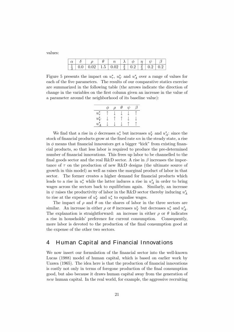
values:

α δ ρ θ n λ φ η ψ β13 0.0 0.02 1.5 0.02 2

3 0.2 23 0.2 0.2

Figure 5 presents the impact on u∗τ , u∗Y and u∗A over a range of values for

each of the five parameters. The results of our comparative statics exerciseare summarized in the following table (the arrows indicate the direction ofchange in the variables on the first column given an increase in the value ofa parameter around the neighborhood of its baseline value):

φ ρ θ ψ β

u∗τ ↑ ↓ ↓ ↓ ↑u∗Y ↓ ↑ ↑ ↓ ↓u∗A ↓ ↓ ↓ ↑ ↑

We find that a rise in φ decreases u∗τ but increases u∗Y and u∗A: since the

stock of financial products grow at the fixed rate κn in the steady state, a risein φ means that financial innovators get a bigger “kick” from existing finan-cial products, so that less labor is required to produce the pre-determinednumber of financial innovations. This frees up labor to be channelled to thefinal goods sector and the real R&D sector. A rise in β increases the impor-tance of τ on the production of new R&D designs (the ultimate source ofgrowth in this model) as well as raises the marginal product of labor in thatsector. The former creates a higher demand for financial products whichleads to a rise in u∗τ while the latter induces a rise in u∗A in order to bringwages across the sectors back to equilibrium again. Similarly, an increasein ψ raises the productivity of labor in the R&D sector thereby inducing u∗Ato rise at the expense of u∗Y and u

∗τ to equalise wages.

The impact of ρ and θ on the shares of labor in the three sectors aresimilar. An increase in either ρ or θ increases u∗Y but decreases u

∗τ and u

∗A.

The explanation is straightforward: an increase in either ρ or θ indicatesa rise in households’ preference for current consumption. Consequently,more labor is devoted to the production of the final consumption good atthe expense of the other two sectors.

4 Human Capital and Financial Innovations

We now insert our formulation of the financial sector into the well-knownLucas (1988) model of human capital, which is based on earlier work byUzawa (1965). The idea here is that the production of financial innovationsis costly not only in terms of foregone production of the final consumptiongood, but also because it draws human capital away from the generation ofnew human capital. In the real world, for example, the aggressive recruiting

21

of the best graduates from each cohort by financial powerhouses preventssuch talent from being channelled into academia and the teaching profession.

In this model, we examine the optimum allocation of human capitalbetween the final goods, financial and human capital sectors and observehow this varies according to the elasticities and productivity parameters ofthe various inputs in these sectors.

The representative consumer’s problem in this model is

maxC(t),uY (t),uτ (t)

U0 =

Z ∞

0

C (t)1−θ − 11− θ e−ρtdt, (65)

subject to

K (t) =τ (t)

H (t)κ

hAK (t)α (uY (t)H (t))

1−α −C (t)i− δK (t) , (66)

τ (t) = F [uτ (t)H (t)]λ τ (t)φ , (67)

H (t) = D [1− uY (t)− uτ (t)]H (t)− δH (t) . (68)

Note that α ∈ (0, 1), {uY (t) , uτ (t)} ∈ [0, 1] ∀t, {θ, ρ, δ, n} > 0, λ ∈ (0, 1]and φ ∈ [0, 1].

To arrive at the steady-state solutions, we first define the following threevariables ω ≡ K/H, χ ≡ C/K and ζ ≡ τ/Hκ. In the steady state, werequire the output-capital ratio given by

Y

K= Aωα−1u1−αY , (69)

to remain constant. This implies, from equation (69), that

Y

Y− KK= (α− 1) ω

ω+ (1− α) uY

uY= 0. (70)

We also require that uY /uY = 0 in the steady state. Hence, ω/ω = 0in order to satisfy equation (70). This then suggests that K/K = H/Hin the steady state. Furthermore, it is assumed that χ/χ = ζ/ζ = 0 inthe steady state. Hence, these assumptions imply that to have a balancedgrowth path, we must have Y /Y = K/K = C/C = γH and τ/τ = κγH inthe steady state, where γH ≡ H/H and κ = λ/ (1− φ). The growth rateis now determined endogenously instead of being equal to some exogenouspopulation growth rate, as was the case in the first two models.

The model is solved in terms of the five unknowns ω, χ, ζ, uY and uτ .The five equations needed to pin down the solutions to these variables aregiven by ω/ω = 0, χ/χ = 0, ζ/ζ = 0, uY /uY = 0 and uτ/uτ = 0. Thesefive conditions lead to the following equations respectively:

22

ζAωα−1u1−αY − ζχ = γ∗H + δ, (71)

ζAαωα−1u1−αY = ρ+ θγ∗H + δ,

Fuλτ ζφ−1 =

λγ∗H1− φ , (72)

ζAαωα−1u1−αY − γ∗H − δ =Duτ +

DuY1− α

£(1− α− κ) + κ ¡ζ−1A−1ω1−αuα−1Y

¢ζχ¤, (73)

λγ∗τ1− α

uYuτ

£1− ¡ζ−1A−1ω1−αuα−1Y

¢ζχ¤− λγ∗H =

Duτ +DuY1− α

£(1− α− κ) + κ ¡ζ−1A−1ω1−αuα−1Y

¢ζχ¤. (74)

Using equations (71) to (74), we obtain the following solutions for uτ , uY ,uH , ζ, χ and ω:

u∗τ =λγ∗HD

Φ

Γ−Φ , (75)

u∗Y =ρ+ (θ − 1) γ∗H

D

Γ

Γ−Φ , (76)

u∗H =[D − ρ− (θ − 1) γ∗H ]Γ− [D + λγ∗H ]Φ

D (Γ−Φ) , (77)

ζ∗ =

"F

γ∗τ

µλγ∗HD

Φ

Γ−Φ¶λ# 1

1−φ(78)

χ∗ =ρ+ (θ − α) γ∗H + (1− α) δ

α

×"γ∗τF

µD

λγ∗H

Γ−ΦΦ

¶λ# 11−φ

, (79)

ω∗ =

Aα

ρ+ θγ∗H + δ

"F

γ∗τ

µλγ∗HD

Φ

Γ−Φ¶λ# 1

1−φ

11−α

×ρ+ (θ − 1)γ∗H

D

Γ

Γ−Φ , (80)

where γ∗τ = κγ∗H , γ∗H is the root of

Du∗H − δ = γ∗H , (81)

23

and

Γ ≡ (1− α) (ρ+ θγ∗H + δ) [ρ+ (θ + λ− 1)γ∗H ] ,Φ ≡ κα (γ∗H + δ) [ρ+ (θ − 1) γ∗H ] .

Note that γ∗H is the value of H/H in the steady state which yields thesteady-state growth rate of the economy. It is apparent from equation(81) that γ∗H = f (α, δ, ρ, θ,φ,D). Although it is impossible to obtain γ∗Hin analytic form, we use numerical techniques for its solution and performcomparative statics numerically using the following set of baseline values forthe parameters:

α δ ρ θ λ φ A D13 0.05 0.02 1.5 2

3 0.2 1 0.15

The simulation results are presented in the figures below. Figure 6 presentsthe graphs for the shares of human capital. The results for γ∗H are alsopresented in Figure 7 to help analyze the size of the impact.

The set of baseline values yield a steady-state growth rate, γ∗H , of 4.17%approximately. The matrix below provides an overview of the direction ofchange in γ∗H as well as the three shares of human capital u∗τ , u∗Y and u

∗H ,

given an increase in α, δ, ρ, θ, φ and D around the neighborhood of theirbaselines values.

α δ ρ θ φ D

γ∗H ↓ ↓ ↓ ↓ ↓ ↑u∗τ ↑ ↓ ↓ ↓ ↑ ↑u∗Y ↑ ↓ ↑ ↑ ↑ ↓u∗H ↓ ↑ ↓ ↓ ↓ ↓

An increase in α raises the marginal product of human capital in thefinal goods sector. Since wages must equate across all markets for humancapital in equilibrium according to its marginal product, the share of humancapital in the final goods sector must rise relative to the share in the othersectors. Our results show that the rise comes at the expense of a fall in u∗Hthus leading to a fall in γ∗H . An increase in δ ceteris paribus decreases γ

∗H

since it affects directly the accumulation of human capital. However, giventhat both physical and human capital accumulation depend on the stock ofhuman capital, more human capital is needed in the human capital sectorto counteract the higher rate of depreciation, i.e. u∗H increases. This hasthe opposite effect of raising γ∗H . Our simulations indicate that the formereffect dominates the latter.

An increase in either ρ or θ decreases γ∗H . Both have the effect of favoringcurrent consumption vis-a-vis future consumption, leading to more humancapital being channelled to the final goods sector at the expense of the

24

other two sectors. Naturally, the fall in u∗H then leads to a fall in γ∗H .An increase in φ increases the marginal product of human capital in thefinancial innovations sector. In order to bring the marginal products backto equilibrium across the sectors, the share of human capital in the financialinnovations sector has to rise relative to the share in the other sectors. Ourresults indicate that u∗H falls while u

∗τ and u

∗Y increase. The fall in u

∗H hence

causes γ∗H to fall.

0.0

0.1

0.2

0.3

0.4

0.5

0.6

0.7

0.25 0.30 0.35 0.40 0.45 0.50

alphautauuYuH

0.0

0.1

0.2

0.3

0.4

0.5

0.6

0.7

0.03 0.04 0.05 0.06 0.07

deltautauuYuH

0.0

0.1

0.2

0.3

0.4

0.5

0.6

0.7

0.015 0.020 0.025 0.030

rhoutauuYuH

0.0

0.2

0.4

0.6

0.8

1.0

1.0 1.2 1.4 1.6 1.8 2.0 2.2

thetautauuYuH

0.0

0.1

0.2

0.3

0.4

0.5

0.6

0.7

0.15 0.20 0.25 0.30

phiutauuYuH

0.0

0.1

0.2

0.3

0.4

0.5

0.6

0.7

0.10 0.12 0.14 0.16 0.18 0.20 0.22

DutauuYuH

Figure 6: Simulated Comparative Statics

Finally, an increase in the level of productivity in the education sector,D,

25

has a direct effect of raising the rate of human capital accumulation and thusγ∗H . On the other hand, our simulations indicate a rise in D also channelsmore human capital to the financial innovations sector at the expense of theother two, which has the opposite effect on γ∗H . It appears that the formereffect dominates the latter in our simulations.

0.025

0.030

0.035

0.040

0.045

0.050

0.055

0.060

0.8 1.0 1.2 1.4

Proportion of Baseline Valuesalphadelta

Stea

dy-S

tate

Gro

wth

Rat

e

0.02

0.03

0.04

0.05

0.06

0.07

0.08

0.09

0.8 1.0 1.2 1.4

Proportion of Baseline Valuesrhotheta

Stea

dy-S

tate

Gro

wth

Rat

e

0.0420

0.0425

0.0430

0.0435

0.0440

0.0445

0.0450

0.8 1.0 1.2 1.4

Proportion of Baseline Value of phi

Stea

dy-S

tate

Gro

wth

Rat

e

0.00

0.02

0.04

0.06

0.08

0.10

0.8 1.0 1.2 1.4

Proportion of Baseline Value of D

Stea

dy-S

tate

Gro

wth

Rat

e

Figure 7: Impact of Model Parameters on the Steady-State Growth Rate

5 Policy Implications

Our model with technological progress suggests that government subsidiesfor financial innovations may raise the steady-state level of capital and out-put per capita through its effect on the rate of technological innovations.With these subsidies, the financial sector develops more rapidly (its ma-turity being measured by the stock of financial products) and assists thereal R&D sector more capably through its venture capital role. However,as none of the parameters in the financial innovations equation affect thesteady-state growth rate of the economy, subsidies have level but not long-run growth effects.

Deregulation of the financial sector may lead to increased productivity offinancial innovators (captured in our model by a rise in F ), which raises thesteady-state per-capita capital stock and output but not their growth rates.(We can show that when F is too low, the economy may never achieve a 100per cent transformation of savings into investment, i.e. ξ < 1 in the steady

26

state.) Similarly, opening the financial sector of a less developed economy toleading-edge financial firms from advanced countries will enable a transferof financial expertise from the more advanced country to the less developedone, allowing the latter to raise its F parameter and thereby attain itssteady-state sooner while achieving a higher level of GDP per capita. Thiseffect is not to be confused with the issue of increasing capital flows betweencountries.

The results from our model with endogenous human capital accumula-tion suggest that government policies which affect the productivity of theeducation sector raises the long-run growth rate of the economy. However,varying the exponent on the spillover effect of existing financial products onfinancial innovations has no impact on the steady-state growth rate in ourmodel with endogenous technological progress. So perhaps we can arguethat a government intent on generating high long-run growth should focusits attention and direct its subsidies more towards the educational sectorrather than the technological or financial sectors.

6 Conclusion

In this paper, we set out to investigate how the extraordinary expansion inthe variety of financial products and the increasing sophistication of the fi-nancial sector lead to rising affluence in the context of an endogenous growthmodel. The channels we explored are capital accumulation and technologicalinnovation.

We developed a formulation of the financial sector which was then em-bedded in three growth models, including one in which technological progressis modelled endogenously as an expansion in the variety of intermediategoods and another in which a broad definition of capital used in the produc-tion of final goods includes both physical and human capital. Our financialsector comprises financial innovators and financial intermediaries. Financialinnovators utilize labor (or human capital) and the existing catalog of fi-nancial products to develop new financial products and services. Financialintermediaries then purchase these innovations to improve their efficiency intransforming household savings into productive investment by firms. In themodel with endogenous technological progress, we also allowed for spilloversfrom financial innovations into the production of new designs in the realR&D sector.

By solving for the steady-state values of the variables of interest andanalyzing the resulting comparative statics, we showed that financial inno-vations ultimately affect the long-run growth rate only through the channelof technological innovation The rise in transformative efficiency of savingsinto new capital through the adoption of financial innovations slows andeventually comes to a halt in the steady state, so that an increase in the

27

marginal productivity of the financial sector leads to growth effects on thetransitional path to the steady state but only level effects in the long run.We then discussed the policy implications arising from these results.

Extensions to be explored and future research plans include opening theeconomy to allow for capital inflows and outflows, as well as formulatinga model with financial innovation, endogenous technological progress andendogenous human capital accumulation.

References

Acemoglu, D., and F. Zilibotti (1997): “Was Prometheus Unbound byChance? Risk, Diversification and Growth,” Journal of Political Econ-omy, 105, 709—751.

Aghion, P., and P. Howitt (1992): “A Model of Growth Through Cre-ative Destruction,” Econometrica, 60, 323—351.

Arestis, P., and P. O. Demetriades (1997): “Financial Developmentand Economic Growth: Assessing the Evidence,” Economic Journal, 107,783—799.

Barro, R., and X. Sala-I-Martin (1995): Economic Growth. McGraw-Hill, New York.

Bencivenga, V. R., and B. D. Smith (1991): “Financial Intermediationand Endogenous Growth,” Review of Economic Studies, 58, 195—209.

(1993): “Some Consequences of Credit Rationing in an EndogenousGrowth Model,” Journal of Economic Dynamics and Control, 17, 97—122.

Bencivenga, V. R., B. D. Smith, and R. M. Starr (1995): “Trans-action Costs, Technological Choice and Endogenous Growth,” Journal ofEconomic Theory, 67, 153—177.

(1996): “Equity Markets, Transactions Costs and Capital Accu-mulation: An Illustration,” World Bank Economic Review, 10, 241—265.

Berthelmy, J. C., and A. Varoudakis (1996): “Economic Growth, Con-vergence Clubs and the Role of Financial Development,” Oxford EconomicPapers, 48, 300—328.

Betts, C., and J. Bhattacharya (1998): “Unemployment, Credit Ra-tioning and Capital Accumulation: A Tale of Two Frictions,” EconomicTheory, 12(3), 489—518.

Blackburn, K., and V. T. Y. Hung (1998): “A Theory of Growth,Financial Development and Trade,” Economica, 65, 107—124.

28

Bose, N., and R. Cothren (1996): “Equilibrium Loan Contracts andEndogenous Growth in the Presence of Asymmetric Information,” Journalof Monetary Economics, 38, 363—376.

Boyd, J., and B. D. Smith (1996): “The Coevolution of the Real andFinancial Sector in the Growth Process,” World Bank Economic Review,10, 371—396.

Buiter, W. H., and K. M. Kletzer (1995): “Capital Mobility, FiscalPolicy and Growth under Self-Financing of Human Capital Formation,”Canadian Journal of Economics, 28, S163—S194.

Cass, D. (1965): “Optimum Growth in an Aggregative Model of CapitalAccumulation,” Review of Economic Studies, 32, 233—240.

Chiang, A. C. (1992): Elements of Dynamic Optimization. McGraw-Hill,New York.

de Gregorio, J. (1996): “Borrowing Constraints, Human Capital Accu-mulation and Growth,” Journal of Monetary Economics, 37, 49—71.

de la Fuente, A., and J. M. Marin (1996): “Innovation, Bank Mon-itoring and Endogenous Financial Development,” Journal of MonetaryEconomics, 38, 269—301.

Demetriades, P. O., and K. A. Hussein (1996): “Does Financial Devel-opment Cause Economic Growth? Time-Series Evidence from 16 Coun-tries,” Journal of Development Economics, 51, 387—411.

Devereux, M. B., and G. W. Smith (1994): “International Risk Sharingand Economic Growth,” International Economic Review, 35, 535—550.

Dixit, A., and J. E. Stiglitz (1977): “Monopolistic Competition andOptimum Product Diversity,” American Economic Review, 67, 297—308.

Gertler, M. (1988): “Financial Structure and Aggregate Economic Activ-ity: An Overview,” Journal of Money, Credit and Banking, 20, 559—588.

Greenwood, J., and B. Jovanovic (1990): “Financial Development,Growth and the Distribution of Income,” Journal of Political Economy,98, 1076—1107.

Greenwood, J., and B. D. Smith (1997): “Financial Markets in Devel-opment and the Development of Financial Markets,” Journal of EconomicDynamics and Control, 21, 145—181.

Grossman, G. M., and E. Helpman (1991a): Innovation and Growth inthe Global Economy. MIT Press, Cambridge, Massachussetts.

29

(1991b): “Quality Ladders and Product Cycles,” Quarterly Journalof Economics, 106, 557—586.

(1991c): “Quality Ladders in the Theory of Growth,” Review ofEconomic Studies, 58, 43—61.

Japelli, T., and M. Pagano (1994): “Saving, Growth and Liquidity Con-straints,” Quarterly Journal of Economics, 108, 83—109.

Jones, C. I. (1995): “Research and Development Based Models of Eco-nomic Growth,” Journal of Political Economy, 103, 759—784.

King, R. G., and R. Levine (1993a): “Finance and Growth: SchumpeterMight Be Right,” Quarterly Journal of Economics, 108, 717—737.

(1993b): “Finance, Entrepreneurship and Growth: Theory andEvidence,” Journal of Monetary Economics, 32, 513—542.

Koopmans, T. C. (1965): “On the Concept of Optimal Economic Growth,”in The Economic Approach to Development Planning. North-Holland,Amsterdam.

Levine, R. (1997): “Financial Development and Economic Growth: Viewsand Agenda,” Journal of Economic Literature, 35, 688—726.

Levine, R., and S. Zevos (1998): “Stock Markets, Banks and EconomicGrowth,” American Economic Review, 88, 537—558.

Lucas, Robert E., J. (1988): “On the Mechanics of Economic Develop-ment,” Journal of Monetary Economics, 22, 3—42.

Ma, C. H., and B. D. Smith (1996): “Credit Market Imperfections andEconomic Development: Theory and Evidence,” Journal of DevelopmentEconomics, 48, 351—387.

Obstfeld, M. (1994): “Risk-Taking, Global Diversification and Growth,”American Economic Review, 84, 1310—1329.

Pagano, M. (1993): “Financial Markets and Growth: An Overview,” Eu-ropean Economic Review, 37, 613—622.

Romer, P. M. (1990): “Endogenous Technological Change,” Journal ofPolitical Economy, 98, S71—S102.

Saint-Paul, G. (1992): “Technological Choice, Financial Markets and Eco-nomic Development,” European Economic Review, 36, 763—781.

Shi, S. (1996): “Asymmetric Information, Credit Rationing and EconomicGrowth,” Canadian Journal of Economics, 29, 665—687.

30

Solow, R. M. (1956): “A Contribution to the Theory of EconomicGrowth,” Quarterly Journal of Economics, 70, 65—94.

Swan, T. W. (1956): “Economic Growth and Capital Accumulation,” Eco-nomic Record, 32, 334—361.

Tsiddon, D. (1992): “A Moral Hazard Trap to Growth,” InternationalEconomic Review, 33, 299—321.

Uzawa, H. (1965): “Optimum Technical Change in an Aggregative Modelof Economic Growth,” International Economic Review, 6, 12—31.

A Mathematical Proofs

Proof for Proposition 2. The representative consumer in the decentral-ized economy seeks to

maxc,uY

U0 =

Z ∞

0

c1−θ − 11− θ e−ρtdt,

subject to

V = rVK +wY uYL+wτuτL+ πτ −C,K = ξV ,

τ = F (uτL)λ ,

where V is the flow of savings accumulated by households, rV is the rateof interest paid by financial intermediaries to households on the stock ofsavings that has been successfully transformed i.e. K, πτ is the monopolis-tic profits earned by the producers of financial products, τ , and F ≡ Fτφ.The equation for τ differs from that in the social planner’s case because thefinancial innovators do not internalize the spillovers from existing financialproducts. The monopolistic profits, equal to revenue Pτ τ less labor costswτuτL, accrue to households who also own the firms in the financial innova-tions sector. In every period, financial intermediaries earn rKK from theirloans to firms which is just enough to cover their payments, rVK and Pτ τ ,to households (for their deposits) and the financial innovations sector (forthe financial products) respectively. In equilibrium, wages are equal acrossall labor markets, i.e. wY = wτ = w. These conditions together yield thefollowing households budget constraint

K = ξ (rKK + wuY L−C) .Solving the Hamiltonian then yields

u∗τ =Γ

Γ+Φ,

31

where Γ ≡ αλnγ∗τ , Φ ≡ (1 − α)(ρ + n) [ρ+ γ∗τ ] and γ∗τ = λn/ (1− φ). Ex-pressing the ratio of the two shares of labor, (u∗τ/u∗Y )

DC , as a function of(u∗τ/u∗Y )

SP , where DC and SP denote the decentralized economy and thesocial planner respectively, we haveµ

u∗τu∗Y

¶DC=(1− φ)(ρ+ λn)(1− φ)ρ+ λn

µu∗τu∗Y

¶SP,

which shows that u∗DCτ < u∗SPτ as long as φ > 0. The divergence betweenthe two increases as φ increases.

Proof for Proposition 3. The partial total derivative of u∗τ withrespect to φ is

§u∗τ§φ =

∂u∗τ∂Γ

∂Γ

∂φ+∂u∗τ∂Φ

∂Φ

∂φ

=ΓΦ

(Γ+Φ)2 (1− φ) > 0.

Note that ∂Γ∂φ = 0.Proof for Proposition 4. The partial total derivative of u∗τ with

respect to ρ is

§u∗Y§ρ =

∂u∗τ∂Γ

∂Γ

∂ρ+∂u∗τ∂Φ

∂Φ

∂ρ

= − ΓΦ

(Γ+Φ)22ρ+ (1 + λ)n+ δ

(ρ+ λn)(ρ+ n+ δ)< 0,

Note that ∂Γ∂ρ = 0.Proof for Proposition 5. The partial total derivative of u∗τ with

respect to θ is

§u∗Y§θ = 0.

B The Decentralized Economy in the Model withTechnological Progress

The Hamiltonian is

H ≡ c1−θ − 11− θ e−ρt + νξ (rKK + wuY L+ wuAL+Rττ

+Aπx + πA − PABuηALητβ −C´

+µFuλτLλ + υBuηAL

ητβ.

32

Solving the Hamiltonian yields

u∗τ =Γ

Γ+Φ,

where Γ ≡ Γ1Γ2 + Γ3 and

Γ1 ≡ α2 (n+ γ∗A)(1− α) ¡ρ+ n+ θγ∗A¢ ,

Γ2 ≡ ρ+ θγ∗Aρ+ (θ + αη) γ∗A

,

Γ3 ≡ αβγ∗Aρ+ (θ + αη) γ∗A

,

Φ ≡ ρ+ λn+ (θ − 1) γ∗Aλγ∗τ

,

u∗Y = Γ2 (1− u∗τ ) ,u∗A = (1− Γ2) (1− u∗τ ) .

Note that depreciation is dropped here for simplicity.

C The Social Planner’s Problem in the Model withTechnological Progress

The Hamiltonian is:

H ≡ c1−θ − 11− θ e−ρt + ν

h τLκ¡KαA1−αu1−αY L1−α −C¢− δKi (82)

+µFuλτLλτφ + υB (1− uY − uτ )η LητβAψ,

where the control variables are c, uY and uτ , the state variables are K, τand A, and ν, µ and υ are the costate variables associated with K, τ and Arespectively. The first-order conditions are:

∂H

∂C= c−θe−ρt − ντ = 0, (83)

∂H

∂uy= ντKαA1−α (1− α)u−αY L1−α−κ − υBη (1− uY − uτ )η−1 LητβAψ

= 0, (84)∂H

∂uτ= µFλuλ−1τ Lλτφ − υBη (1− uY − uτ )η−1LητβAψ = 0. (85)

33

ν = −∂H

∂K= −ν ¡ταKα−1A1−αu1−αY L1−α−κ − δ¢ , (86)

µ = −∂H

∂τ= −ν

µKαA1−αu1−αY L1−α−κ − C

Lκ

¶− µFuλτLλφτφ−1

−υB (1− uY − uτ )η Lηβτβ−1Aψ, (87)

υ = −∂H

∂A= −ντKα (1− α)A−αu1−αY L1−α−κ

−υB (1− uY − uτ )η LητβψAψ−1. (88)

In addition, the growth rates of the state variables are given by

K

K=

τ

Lκ

µKα−1A1−αu1−αY L1−α − C

K

¶− δ, (89)

τ

τ= FuλτL

λτφ−1, (90)

A

A= B (1− uY − uτ )η LητβAψ−1. (91)

and the transversality conditions are

limt→∞ν (t)K (t) = 0, (92)

limt→∞µ (t) τ (t) = 0, (93)

limt→∞υ (t)A (t) = 0. (94)

To arrive at the steady-state solutions, we first define the following threevariables k ≡ K/AL, χ ≡ C/K and ξ ≡ τ/Lκ. In the steady state, werequire the output-capital ratio given by

Y

K= kα−1A1−αu1−αY , (95)

to remain constant. This implies, from equation (??), that

Y

Y− KK= (α− 1) k

k+ (1− α) A

A+ (1− α) uy

uy= 0. (96)

In addition, uY /uY = 0 in the steady state. Hence, k/k = A/A in orderto satisfy equation (96). This then suggests that K/K = A/A + n, givenequation (56), in the steady state. Furthermore, it is assumed that χ/χ =ξ/ξ = 0 in the steady state. Hence these assumptions imply that a balancedgrowth path requires Y /Y = K/K = C/C = A/A+n and τ/τ = κn in thesteady state.

With endogenous technological progress embedded in the model, thegrowth rate of output is now augmented by the growth rate of technology.Again, this result is comparable to that of the Cass-Koopman’s model with

34

technological progress. The presence of technological progress offsets thediminishing marginal product of physical capital, thereby continually raisingthe productivity level of labor.

To solve for A/A, we impose the conditions that A/A and τ/τ are con-stant in the steady state. Let γA ≡ A/A and γτ ≡ τ/τ . These conditionsimply that

γAγA

= −η uY + uτ1− uY − uτ + ηn+ (ψ − 1)γA + βγτ = 0, (97)

γτγτ

= λuτuτ+ λn+ (φ− 1) γτ = 0. (98)

Since uY = uτ = 0 in the steady state, solving equations (97) and (98) forγA and γτ thus yields

γ∗A =[(1− φ) η + λβ]n(1− φ) (1− ψ) , (99)

γ∗τ =λn

1− φ . (100)

D Mathematical Notation

C = consumptionρ = subjective discount rateθ = coefficient of risk-aversion in the utility functionδ = rate of depreciationt = timeK = physical capitalL = laborn = rate of growth of the labor forceuY = share of labor (or human capital) devoted to production of final con-sumption gooduτ = share of labor (or human capital) devoted to production of financialinnovationsuA = share of labor devoted to R&D of new technological designsuH = share of labor devoted to production of human capitalH = stock of human capitalτ = stock of financial innovationsξ ≡ τ/Lκ = efficiency of intermediation between savings and investmentς ≡ τ/Hκ = number of financial innovations per adjusted unit of humancapitalχ ≡ C/K = consumption-capital ratiok ≡ K/L = capital-labor ratiobk ≡ K/AL = technology-augmented capital-labor ratioω ≡ K/H = physical to human capital ratio

35

γ∗τ = steady-state growth rate of the stock of financial innovationsγ∗A = steady-state growth rate of the number of intermediate goodsγ∗H = steady-state growth rate of human capitali = index of intermediate goodsA = number of intermediate goodsx = quantity of any intermediatewj = wage rate in sector jrV = interest rate on transformed savings earned by householdsrK = interest rate paid by financial intermediaries by borrowers (firms)p(xi) = price of intermediate good iπx = profits earned by a producer of an intermediate goodπτ = profits earned by a financial innovatorα = capital’s share of income generated in final goods productionλ = elasticity of financial innovation production with respect to laborφ = elasticity of financial innovation production with respect to the existingstock of financial productsκ = a measure of the average degree of rivalry in financial productsη = elasticity of R&D production with respect to laborψ = elasticity of R&D production with respect to the existing stock of R&Ddesignsβ = elasticity of R&D production with respect to the stock of financialinnovations

36